spectral methods for investigating solutions to partial

Spectral methods for investigating solutions topartial differential equations

Benson MuiteAcknowledgements

J. Ball, S. Balakrishnan, G. Chen, B. Cloutier, R. Kohn, N. Li,B. Palen, P. Plechac, P. Rigge, W. Schlag, A. Souza, N.

Trefethen, M. Vanmoer, J. West

[email protected]/˜muite

6 February 2013

[email protected]

www.math.lsa.umich.edu/~muite

Outline

The Kohn-Muller functionalThe Aviles-Giga functionalThe 2D Navier Stokes equationKlein-Gordon equationConclusion

Section 1: Computations of the Kohn-Muller model

The sharp interface Kohn-Muller modelThe smooth interface Kohn-Muller modelComputational results

Simplified model which may capture twinning at aboundary

Twinning in Copper Aluminum Nickel (picture by Chu andJames)

The Kohn-Muller model

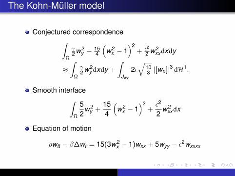
Conjectured correspondence∫Ω

γ2 w2

y + 154

(w2

x − 1)2

+ ε2

2 w2xx dxdy

≈∫

Ω

γ2 w2

y dxdy +

∫Jwx

2ε√

103 |[wx ]|3 dH1.

Smooth interface∫Ω

52

w2y +

154

(w2

x − 1)2

+ε2

2w2

xx dx

Equation of motion

ρwtt − β∆wt = 15(3w2x − 1)wxx + 5wyy − ε2wxxxx

Numerical Results for the Kohn-Muller model

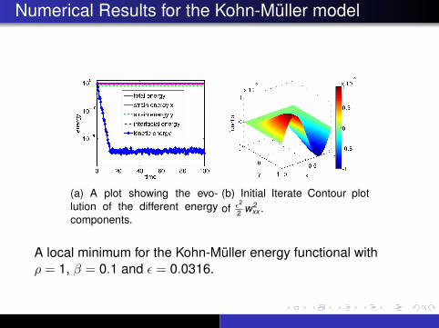
(a) A plot showing the evo-lution of the different energycomponents.

(b) Initial Iterate Contour plotof ε2

2 w2xx .

A local minimum for the Kohn-Muller energy functional withρ = 1, β = 0.1 and ε = 0.0316.


(c) Final iterate. Colours showthe function, w .

(d) Contour plot of 52 w2

y in thefinal iterate.

A local minimum for the Kohn-Muller energy with ρ = 1, β = 0.1and ε = 0.0316.


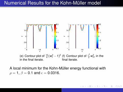
(e) Contour plot of 154 (w2

x − 1)2

in the final iterate.(f) Contour plot of ε2

2 w2xx in the

final iterate.



(g) A plot showing the evo-lution of the different energycomponents.

(h) Initial Iterate Contour plotof ε2

2 w2xx .



(i) Final iterate. Colours showthe function, w .

(j) Contour plot of 52 w2

y in thefinal iterate.

A local minimum for the Kohn-Muller energy with ρ = 1, β = 0.1and ε = 0.001.


(k) Contour plot of 154 (w2

x − 1)2

in the final iterate.(l) Contour plot of ε2

2 w2xx in the

final iterate.


Scaling law predicted by Kohn and Muller for the totalenergy

!"!#

!"!$

!"!!

!"!$

!"!!

!""

!"!

!

%&%'()

*

*

+,-./*0&%'()

1*2-'.3&*%&%'()

4*2-'.3&*%&%'()

5&-%'6.73./*%&%'()

Energy scaling, reference line drawn for ease of comparison.For small ε good agreement with theoretical predictions.

Section 2: Computations of the Aviles-Giga model

The modelThe conjectureComputational results

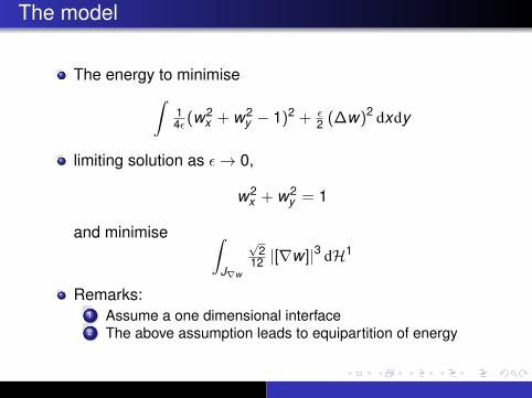
The model

The energy to minimise∫14ε(w

2x + w2

y − 1)2 + ε2 (∆w)2 dxdy

limiting solution as ε→ 0,

w2x + w2

y = 1

and minimise ∫J∇w

√2

12 |[∇w ]|3 dH1

Remarks:1 Assume a one dimensional interface2 The above assumption leads to equipartition of energy

Points which need to be demonstrated for theconjecture to hold

The Γ–limit is infinite unless wxx + wyy = 1 almosteverywhereThe proposed sharp interface limit |∇w |/3 is correctThe asymptotic energy lives on a one dimensional defectset, and lower dimensional singularities carry no energy

DeSimone, Kohn, Muller and Otto

Equation of motion

The energy to minimise∫14(w2

x + w2y − 1)2 + ε2

2 (∆w)2 dxdy

Viscoelastic dynamics

ρwtt − β∆wt

=[wx (w2

x + w2y − 1)

]x

+[wy (w2

x + w2y − 1)

]y− ε2∆2w

Numerical Results for the Aviles-Giga model 1

0 10 20 30 4010−20

10−15

10−10

10−5

100

time

ener

gy

total energystrain energyinterfacial energykinetic energy

(m) A plot showing the evo-lution of the different energycomponents.

00.5

1

−1

0

10

0.005

0.01

xy

func

tion

2

4

6

8

10x 10−3

(n) Initial Iterate

Numerically computed minimizer for the Aviles-Giga energyfunctional with ρ = 1, β = 1.0, ε = 0.05, w(y = ±1) = 0 andwyy (y = ±1) = 0.


00.5

1

−1

0

1−0.5

0

0.5

1

xy

func

tion

0

0.2

0.4

0.6

0.8

(o) Final Iterate

00.5

1

−1

0

10

0.5

1

xy

func

tion

0.1

0.2

0.3

0.4

0.5

0.6

0.7

0.8

0.9

(p) Viscosity solution assum-ing equipartition of energy



!

"

#

#

$ $%& $%' $%( $%) *!*

!$%+

$

$%+

*

$%$+

$%*

$%*+

$%&

(q) Contour plot of interfaceenergy term ε2

2 (∆w)2 in the fi-nal iterate.

x

y

0 0.2 0.4 0.6 0.8 1−1

−0.5

0

0.5

1

0.05

0.1

0.15

0.2

(r) Contour plot of 14 (w2

x +w2y −

1)2 in the final iterate



0 2000 4000 6000 8000 10000

10−20

10−10

100

time

ener

gy


(s) A plot showing the evo-lution of the different energycomponents.

00.5

1

−1

0

1−0.5

0

0.5

xy

func

tion

−0.5

0

0.5

(t) Initial Iterate

Numerically computed minimizer for the Aviles-Giga energyfunctional with ρ = 1, β = 1.0, ε = 0.01,w(y = ±1) = −0.05 sin(2πx) and wyy (y = ±1) = 0.


00.5

1

−1

0

1−0.5

0

0.5

1

xy

func

tion

0

0.2

0.4

0.6

0.8

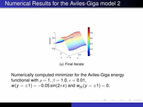
(u) Final Iterate



x

y

0 0.2 0.4 0.6 0.8 1−1

−0.5

0

0.5

1

0.05

0.1

0.15

0.2

0.25

0.3

0.35

0.4

(v) Contour plot of interfaceenergy term ε2

2 (∆w)2 in the fi-nal iterate.

x

y

0 0.2 0.4 0.6 0.8 1−1

−0.5

0

0.5

1

0.02

0.04

0.06

0.08

0.1

0.12

(w) Contour plot of 14 (w2

x +w2y −




0 5 10 15x 104

10−20

10−15

10−10

10−5

100

time

ener

gy


(x) A plot showing the evo-lution of the different energycomponents.

(y) Initial Iterate



(z) Final Iterate



x

y

0 0.2 0.4 0.6 0.8 1−1

−0.5

0

0.5

1

0.05

0.1

0.15

0.2

0.25

0.3

0.35

0.4

() Contour plot of interface en-ergy term ε2

2 (∆w)2 in the finaliterate.

x

y

0 0.2 0.4 0.6 0.8 1−1

−0.5

0

0.5

1

0.05

0.1

0.15

0.2

() Contour plot of 14 (w2

x + w2y −



Result Summary

w(y = ±1) ε∫ 1

4 (w2x + w2

y − 1)2∫

ε2

2 (∆w)2 Total Energyε

0 0.05 0.0235 0.0236 0.9440 0.01 0.00471 0.00471 0.942

−0.005 sin(2πx) 0.05 0.0235 0.0237 0.942−0.005 sin(2πx) 0.01 0.00471 0.00471 0.942

0.05 sin(2πx) 0.05 0.0217 0.0261 0.9560.05 sin(2πx) 0.01 0.00451 0.00458 0.9090.05 sin(2πx) 0.0025 0.000846 0.00132 0.868

Prediction that (Total Energy)/ε= 2√

2/3 ≈ 0.943 if Aviles-Gigaconjecture holds and zero boundary conditions.

Conclusions

Simulations can be a useful tool to test scalingassumptionsFor the Kohn-Muller model, the simulations are inagreement with the modelFor the Aviles-Giga model, the conjecture may not holdwhen non-zero boundary conditions are applied

The 2D Navier-Stokes Equation

Introduction

Consider incompressible case onlyModel for dynamics in a uniform and thin layer of water

ρ

(∂u∂t

+ u · ∇u)

= −∇p + µ∆u

∇ · u = 0.

u(x , y) = (u(x , y), v(x , y)), p pressure, µ viscosity, ρ,density

Vorticity-Streamfunction Formulation

ω = ∇× u =∂v∂x− ∂u∂y

= −∆ψ

ρ

(∂ω

∂t+ u

∂ω

∂x+ v

∂ω

∂y

)= µ∆ω

and

∆ψ = −ω.

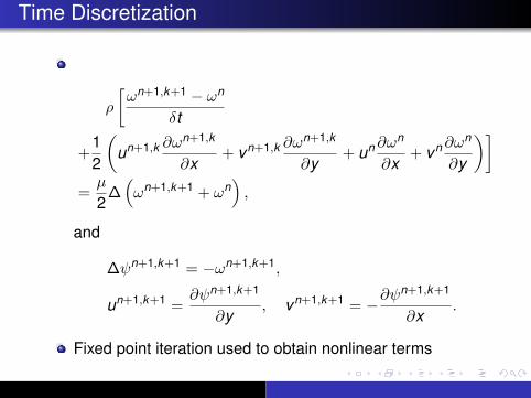
Time Discretization

ρ

[ωn+1,k+1 − ωn

δt

+12

(un+1,k ∂ω

n+1,k

∂x+ vn+1,k ∂ω

n+1,k

∂y+ un ∂ω

n

∂x+ vn ∂ω

n

∂y

)]=µ

2∆(ωn+1,k+1 + ωn

),

and

∆ψn+1,k+1 = −ωn+1,k+1,

un+1,k+1 =∂ψn+1,k+1

∂y, vn+1,k+1 = −∂ψ

n+1,k+1

∂x.

Fixed point iteration used to obtain nonlinear terms

Example Videos

http://www-personal.umich.edu/˜cloutbra/research.html

Simulations on a single NVIDIA Fermi GPU about 20 timesfaster than a 16 core CPU

http://www-personal.umich.edu/~cloutbra/research.html

http://www-personal.umich.edu/~cloutbra/research.html

The Real Cubic Klein-GordonEquation

The Real Cubic Klein-Gordon Equation

utt −∆u + u = |u|2u

E(u,ut ) =

∫12|ut |2 +

12|u|2 +

12|∇u|2 − 1

4|u|4 dx

un+1 − 2un + un−1

(δt)2 −∆un+1 + 2un + un−1

4+

un+1 + 2un + un−1

4

= ±∣∣un∣∣2 un

Parallelization done using 2decomp library for FFT andprocessing independent loops

Relevant Previous Work

Donninger and Schlag (2010) - Study of blowup of radiallysymmetric solutions, 2nd order symplectic schemesBao and Yang (2006) and Yang (2007) 2D simulationsChen (2006) 4th order symplectic schemesHamaza and Zaag (2010) Solutions can only blow up in anODE like manner

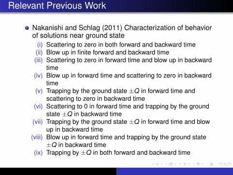
Relevant Previous Work

Nakanishi and Schlag (2011) Characterization of behaviorof solutions near ground state

(i) Scattering to zero in both forward and backward time(ii) Blow up in finite forward and backward time(iii) Scattering to zero in forward time and blow up in backward

time(iv) Blow up in forward time and scattering to zero in backward

time(v) Trapping by the ground state ±Q in forward time and

scattering to zero in backward time(vi) Scattering to 0 in forward time and trapping by the ground

state ±Q in backward time(vii) Trapping by the ground state ±Q in forward time and blow

up in backward time(viii) Blow up in forward time and trapping by the ground state

±Q in backward time(ix) Trapping by ±Q in both forward and backward time

What is Q?

∆Q −Q = Q3.

Example Videos

Dispersion 1Dispersion 2Blow up

Interaction of 2 Solitons

Initial Conditions

u(t = 0) = αQ1 + βQ−1

ut (t = 0) = 2β exp(−x2 − y2 − z2

)cos(4x) cos(6y) cos(8z)

where α ∈ (0,1] and β ∈ (0,1].


0 0.2 0.4 0.6 0.8 10

0.2

0.4

0.6

0.8

1

1.2

1.4

α

β

The × indicate numerical experiments in which there wasblowup and the o indicate numerical experiments for whichthe solution dispersed. As predicted from theory, here is asurface separating solutions which blow up and thosewhich disperse.


Work in reasonable agreement with previous work byDonninger and SchlagAgain, exact criteria to examine for distinguishing betweenblow up and global existence is unclear

Simulations and Videos by Brian Leu, Albert Liu, andParth Sheth

http://www-personal.umich.edu/˜alberliu/

http://www-personal.umich.edu/˜pssheth/

http://www-personal.umich.edu/~alberliu/

http://www-personal.umich.edu/~pssheth/

Conclusion

Easy to program numerical method which can be used tostudy semilinear partial differential equationsMethod parallelizes well on hardware with goodcommunications so a good tool to introduce parallelprogramming ideasResearch tool to investigate and provide conjectures forbehavior of solutions to partial differential equationsResearch tool to investigate computer hardwareperformance and correctnessBetter user interface and integration with visualizationwould help make it easier for those without strongprogramming backgrounds

Acknowledgements and References

The Marie Curie Research Training Network MULTIMATThe HPC-EUROPA projectEPSRC grants, OxMOS “New Frontiers in the Mathematics of Solids”and OxPDE “Oxford Center for Nonlinear Partial Differential Equations”Warwick Center for Scientific ComputingThe Extreme Science and Engineering Discovery Environment(XSEDE), which is supported by National Science Foundation grantnumber OCI-1053575.Hopper at the National Energy Research Scientific Computing CenterSCREMS NSF DMS-1026317The Blue Waters Undergraduate Petascale Education Programadministered by the Shodor foundationThe Division of Literature, Sciences and Arts at the University ofMichiganB.K. Muite, D.Phil. Thesis, University of Oxford 2010G. Chen, B. Cloutier, N. Li, B.K. Muite, P. Rigge and S. Balakrishnan, A.Souza, J. West, “Parallel Spectral Numerical Methods”http://en.wikibooks.org/w/index.php?title=Parallel_Spectral_Numerical_Methods

http://en.wikibooks.org/w/index.php?title=Parallel_Spectral_Numerical_Methods

http://en.wikibooks.org/w/index.php?title=Parallel_Spectral_Numerical_Methods

spectral methods for investigating solutions to partial

Documents