I

rtüii "inali*·'*!' ' *'

EUR 4479 e

i

SPECTRAL PARAMETI ■i$m\

WÊà

m ΐίίΒ-1«

MWfj

léii**1

A.C. Ü

BE ii

tum

\>mm. m

' ä-'ÜBit-f

, ,̂ .

1970

Blip

liill

Η ·■: Joint Nuclear Research Center

Ispra Establishment - Italy

Reactor Physics Department

Research Reactors

i t ,

Kesearcn Keacrors

f tø pf IMI? Iiiiínílíi^'lliw^i»·*»!!!^

«Hf wmSm waëïi

A A A K, f A this document was prepared under the sponsorship ot th of the European Communities^i.fttMä'iwi

Neither the Commission of the European Communities, its contractors nor any person acting on their behalf :

fiSt" ™ fiRá

make any warranty or representation, express or implied, with respect to the accuracy, completeness or usefulness of the information contained in this

fWJftJSû

document, or that the use of 'any information, apparatus, method or process disclosed in this document may not infringe privately owned rights; or

l l å f , „ u , , , , 1 » Ü 1 assume any liability with respect to the use of, or for damages resulting from the use of any information, apparatus, method or process disclosed in this document.

fi Aie

ιΐϋΐ •sír'5¿i'}ll!

This report is on sale at the addresses listed on cover page 4 fS'-iEuflfi'piîMLsfli'iiÎMiW'1 'J*' r'Urt^íSlTSfltislHiilMiMHjTÍ"^

.¡vit­

ut the price of FF 9,45 FB 8 5 - D M 6,20 Lit 1.060 FI. 6,20

ïah When ordering, please quote the EUR number and the title, which are indicated on the cover of each report

1 WMpttIcU *v*r 1 BE

sfliilìl »l^if ie KS? ί MM Printed by Smeets, Brussels Luxembour,

-h Vlililí u # f e e I t ó 1

ouTg, May 1970

K*l*LrV,;íld

»Av

ψ4 This document was reproduced on the basis of the best available copy

tfwi< ¡;KLí W *

EUR 4479 e S P E C T R A L P A R A M E T E R E S T I M A T I O N F O R L I N E A R S Y S T E M I D E N T I F I C A T I O N , by C . L U C I A

Commission of t h e European Communit ies Joint Nuc lea r Research Cen te r - Ispra Establishment (Italy) Reactor Physics Depar tment - Research Reactors Luxembourg, M a y 1970 - 58 Pages - 2 Figures - F B 85

T h e aim of this report is to examine the properties and statistical errors of the estimators of some spectral parameters of stationary, ergodic, linear processes (power and cross-power spectral density, Fourier transform, transfer funct ions) .

In addition, procedures and computing programmes are supplied for the estimation of these parameters by means of the statistical dynamics analyzer S . D . A . - M o d . 040. T h e case of deterministic signals is also taken into consideration.

EUR 4479 e S P E C T R A L P A R A M E T E R E S T I M A T I O N F O R L I N E A R S Y S T E M I D E N T I F I C A T I O N , by C . L U C I A

Commission of the European Communit ies Joint Nuclear Research Center - Ispra Establishment i(Italy) Reactor Physics Depar tment - Research Reactors Luxembourg, M a y 1970 - 58 Pages - 2 Figures - F B 85

T h e aim of this report is to examine the properties ana statistical errors of the estimators of some spectral parameters of stationary, ergodic, linear processes (power and cross-power spectral density, Fourier transrorm, transfer funct ions) .

In addition, procedures and computing programmes are supplied for the estimation of these parameters by means of the statistical dynamics analyzer S .D.A. - Mod . 040. T h e case of deterministic signals is also taken into consideration.

EUR 4479 e S P E C T R A L P A R A M E T E R E S T I M A T I O N F O R L I N E A R S Y S T E M I D E N T I F I C A T I O N , by C . L U C I A

Commission of the European Communit ies Joint Nuclear Research Center - Ispra Establishment (Italy) Reactor Physics Depar tment - Research Reactors Luxembourg, M a y 1970 - 58 Pages - 2 Figures - FB 85

T h e aim of this report is to examine the properties and statistical errors of the estimators of some spectral parameters of stationary, ergodic, linear processes (power and cross-power spectral density, Fourier transrorm, transfer functions) .

In addition, procedures and computing programmes are supplied for the estimation of these parameters by means of the statistical dynamics analyzer S .D .A. - Mod. 040. T h e case of deterministic signals is also taken into consideration.

EUR 4479 e

COMMISSION OF THE EUROPEAN COMMUNITIES

SPECTRAL PARAMETER ESTIMATION FOR LINEAR SYSTEM IDENTIFICATION

by

AC. LUCIA

1970

Joint Nuclear Research Center Ispra Establishment - Italy

Reactor Physics Department Research Reactors

ABSTRACT

The aim of this report is to examine the properties and statistical errors or the estimators of some spectral parameters of stationary, ergodic. linear processes (power and cross-power spectral density. Fourier transform, transfer functions).

In addition, procedures and computing programmes are supplied for the estimation of these parameters by means of the statistical dynamics analyzer S.D.A. - Mod. 040. The case of deterministic signals is also taken into consideration.

KEYWORDS

MATHEMATICS PARAMETERS FOURIER TRANSFORMATIONS COMPUTERS STATISTICS SPECTRA

CONTENTS

INTRODUCTION

1.) SPECTRAL ANALYSIS OF RANDOM SIGNALS

pages

1.1.) Power spectral density estimation 7 1.2.) Cross-power spectral density estimation -\ A 1.3.) Power and cross-power spectral density estimation with

the statistical dynamics analyzer S.D.A 17

2.) SPECTRAL ANALYSIS OF APERIODIC SIGNALS 24

2.1.) Fourier transform estimation 25 2.2.) Fourier transform estimation with the statistical dyna­

mics analyzer S.D.A. 26 2.3.) Energy and cross-energy spectral density estimation .... 3O 2.4.) Energy and cross-energy spectral density estimation with

the statistical dynamics analyzer S.D.A 31

3.) SPECTRAL ANALYSIS OF PERIODIC SIGNALS 33

3.1.) Fourier transform estimation with the statistical dyna­mics analyzer S.D.A 34

3.2.) Power and cross-power spectral density estimation with the statistical dynamics analyzer S.D.A 37

APPENDIX 39

FIGURE CAPTIONS 56

LIST OF TABLES 56

REFERENCES 57

SPECTRAL PARAMETER ESTIMATION FOR LINEAR SYSTEM IDENTIFICATION

INTRODUCTION *)

The techniques for determining the power and cross-power spectral density, the Fourier transforms and the transfer functions assume considerable importance in the identification of a system or

1 2 3 process ) ) ). From these functions it is in fact often pos­sible to arrive at some basic parameters of the system or process un­der examination. For this reason it is interesting to know the characteristics of the estimators we use and the accuracy obtainable with them.

This report studies the statistical properties of some continuous estimators in general use which allow direct determination of Fourier transforms, power and cross-power spectral densities and transfer functions. The determination of these functions is trea­ted categorically for the cases of random signals and of aperiodic and periodic signals.

The estimators we deal with in this work also constitute the algorithms by which are obtained the determinations made on the statistical dynamics analyzer S.D.A. (a general purpose analyzer,

4 designed and built at the Euratom Joint Research Center of Ispra) ) .

In the sections 1.3; 2.3 and 3.2 and in the Appendix, in which processing procedures and computing programmes are given, re­ference is made exclusively to the S.D.A.

Manuscript received on 11 March 1970

1.) SPECTRAL ANALYSIS OF RANDOM SIGNALS

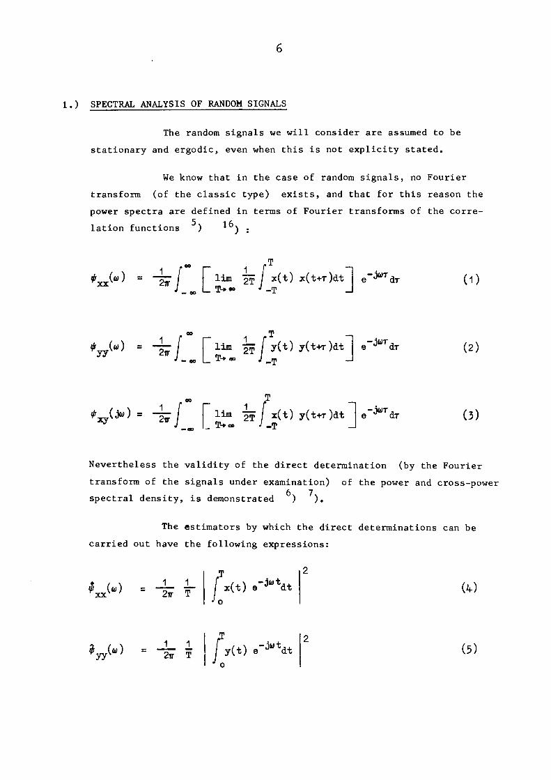
The random signals we will consider are assumed to be

stationary and ergodic, even when this is not explicity stated.

We know that in the case of random signals, no Fourier

transform (of the classic type) exists, and that for this reason the

power spectra are defined in terms of Fourier transforms of the corre­

lation functions ) 16 )

Φ (ω) = if 1 Τ

lim 2T / x(*) x(t+T)dt

_ T-* «e J _φ e­

JWTdT (1)

Φ (ω) yy

co Τ

■—ƒ film ~ fy(t) y(t+r)at e-Jft,TdT (2)

# ^ ( » 1 2π

Τ lim Jr / x(t) y(t-»r)dt T-» ce J _τ

-JWT, β dr (3)

Nevertheless the validity of the direct determination (by the Fourier transform of the signals under examination) of the power and cross-power spectral density, is demonstrated ) ).

The estimators by which the direct determinations can be carried out have the following expressions:

XX 1 j _ 2ir Τ

.Τ c(t) θ -3<iì t

d t (4)

* (ω)

yyv

1 j _ 2ir T y(t) -jut

dt (5)

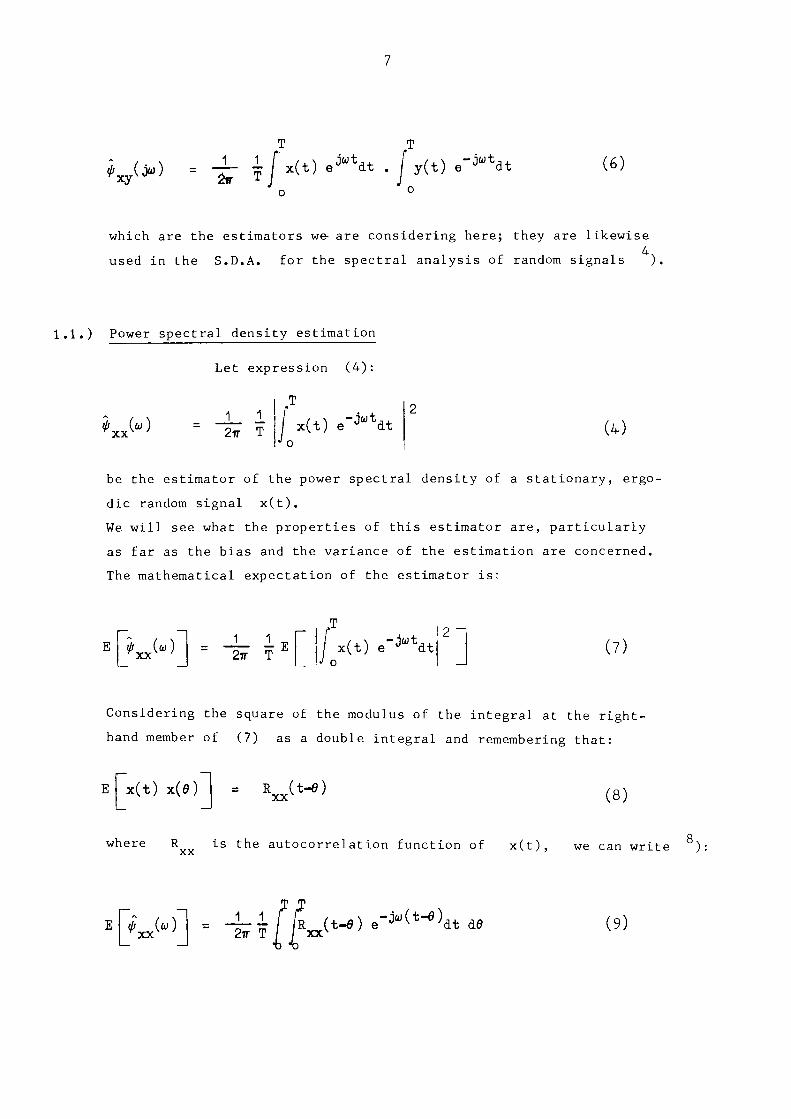
^(¿ω) 1­ ifiítje^dt . fy(t) 2* Τ

rjCüt

dt (6)

which are the estimators we­ are considering here; they are likewise 4

used in the S.D.A. for the spectral analysis of random signals ).

1.1.) Power spectral density estimation

Let expression (4):

Τ

Φ (ω) xx

1 ι 2π Τ

c(t) e"d<üt

dt (4)

be the estimator of the power spectral density of a stationary, ergo­

dic random signal x(t).

We will see what the properties of this estimator are, particularly

as far as the bias and the variance of the estimation are concerned.

The mathematical expectation of the estimator is:

Φ (ω) rxx

■1­ I F

2π Τ E

x(t) e"Jwt

dt (7)

Considering the square of the modulus of the integral at the right­

hand member of (7) as a double integral and remembering that:

E c(t) x(e) R (t­e) xx (8)

where R is the autocorrelation function of x(t), we can write ):

E Φ ( ω ) χ χ

ν ±-lfjí (t-e) e-Jw(t-e)dt dö 2π Τ / / χ χ

ν '

(9)

8

which gives f ina l ly )

■[>»(·>] ­^¡j­^y^r) e­JwTdT (10)

For an analysis time Τ tending to the infinite, wherever the auto­

correlation function can be integrated absolutely, we obtain from (10)ι

lim E

Τ­*«· ƒ«(-)] Η. R (τ) e xx '

-JUT dr = Φ (ω) rxx x ' (H)

i.e. the estimator (4) is unbiased in the limit, but for a finite ana­lysis time Τ , it is biased: that is, it contains a systematic error. Let us now see what the variance of the estimate is:

var *„(-)] E Φ' (u) xxv - E ψ (ω) rxxx (12)

Q where the mathematical expectation of the square of the estimate is ):

E [>„<«: E r J__ 1 2π Τ

x(t) e-^at 2

] 2 ]

τ τ τ. τ = - L —ί ! [ ΓΕ Tx(t) χ(0) χ(τ,) χ(ξ)β'οω^+θ-η'ξ) Ί dt dø dr, ae

1*1* T?b h h Jo L J (13)

the expression at the third member of (13) having been deduced by con­sidering the square of the integral as a double integral, and by using the property of interchangeability of the operation of finding the ma­thematical expectation and the operation of integration.

Remembering that for any four normal variables χ , χ ,

x„, χ. we have ; ; : 3 4

E(xlxax3x4)= EtxiX,) Ε(χ3χ4)+ E(x1x3)E(xax4)+ Ε(χ1χ4)Ε(χ3χ3)­ 2 3^X3X3^ =

= RiaR34+ Ri3Ra4+ » 1 4 ^ 3 - 2 x ^ x , ^ (14)

where R.. is the correlation function of the ith and jth random va­

riables, we obtain from expression (13):

Τ Τ Τ Τ

<Φ2 (ω)) = — i ,

^χχ^ ¡^ ­τβ ¡ο o

Jo

J o

*«<*­*> Rx x

(^

} + Rxx

(t­^

Rxx

(0­^

)+

^ x x ^ ^ ^ x x ^ ­ ^ ­2^

e­J­(t+e­7í­í)at ¿g d7) ^ (15)

Taking into consideration expression (9) , expansion of the right­hand

member of (15) gives:

E[>y«)) 2(E»M(»»)H^ .τ .T

R (t­*) e> ( t + ö )

dt dø xx

x '

O J O

Τ Τ Τ Τ

1 f Γ Γ Ι Ι -juit+θ-η-ξ)

"2 *V W

O JO JO JO

e dt dø dr? άξ (16)

As Τ tends to the infinite, equation (16) becomes;

lim Ε(^(ω)) = Τ-»««

lim 2(ErJxx(«))) T->«°

(17)

so t h a t by v i r t u e of (12) and (17) one can w r i t e :

l im varfj (ω)) = Τ-*00

l im ( Έ{φ (ω)) ) TV»

(18)

10

Hence from (11)

lim var (ίχχ(ω)) Τ-*»

ø2 (ω) XX

(19)

which means that the random variable constituted by the estimator Ψχγ^ω'

does not converge in the mean upon the value Φ (ω ) of the power

spectral density, and the accuracy of the measurement does not improve

with an increase of integration time Τ . The statistical error

thus remains, even with an infinite analysis­time.

Let us however repeat this measurement on successive times, and use then

the estimator:

7 ( \ 1 1 1 ^ χ χ ( ω ) = k 2 7 ?

i=1

t .+T ι

c ( t ) e - j ûJ t

dt

i=1

(20)

which is unbiased in the limit, as estimator (4) was already; in fact:

k

Ε(Λ>)) = Ï^C*«,!0^

i=1

i xx (21)

and remembering ( i l ) :

l i m E ^ χ χ

( ω ))

=

T->°°

1_

k φ . ( ω ) = Φ (ω) (22)

i=1

As far as the variance of the new estimator is concerned, we must bear

in mind that if the initial instants t. of each integration are spa­

ced sufficiently so that the k determinations can be considered inde­

1 ? pendent, one can write

1^) 13

) :

var (^χχΟ")) = — var k C¿_») XX,1

(23)

11

by which, for ( 19 ) , we have:

l im var ( ^ ^ ( ω ) ) = T-+0O

¿e>) X X (24)

which clearly means that:

lim var (^ (ω)) = lim £ «^U» ) = °

T­> °° k­» °°

k­»°°

(25)

As for an infinite analysis time Τ , the estimator (20) is unbia­

sed (so that mean square arror and variance of the estimate have the

same value), expression (25) means also that estimator (20) is

consistent for infinite values of both Τ and k.

It will be observed that the variance of the estimator tends to zero,

when k tends to be infinite, even if Τ remains finite, while

the mean square error tends to a nonzero value owing to the bias of the

estimate.

Equation (25) has been deduced by considering k indepen­

dent measurements. Let us take, on the other hand, the general case

of correlated measurements:

var Ax<w) = E k£>> - E ΛΦ (ω)

k xx

X i 7,ww)2] - [

E [À>>

i=1

(26)

t h a t i s , developing the square of the summation:

k_ k

var(kíxx(W))= s ß r ¿ ^ ( « V ΈτΣ+χχ,±(ω)**χΛω)

i=1 i , j = 1 i * j

{E[Âx^ J

( 27 ;

12

If we consider the determinations φ .(u) rxx,i

and remember that, for two random variables 9

write ):

as random variables

ζ and w wa can

E(z') = _ a

a" + ζ ζ

E( ζ w ) = α rs (28)

an = R ( 11 zw

v τ) = z.w + ρ (τ) \ C (0)C (θ) = i.w + ρ (τ) σ σ zw' ζζ

ν wvr *

yzw

v y ζ w

where α is the moment of order r+s, equation (27) can be ex· rs

n

pressed as:

' iJvV(o>)) = £ ­k xx var Φ .(ω) + E k*xx^

2Ì J > + ^ ί ,Ä (ω )

+ - v a r *~ Λ«>) XX,χ

ρ . / τ ) . (E ,0 (ω) k xx

s

(29)

from which we obtain the final result:

var k¿xx(w) var Φ .(ω)

_ —

1 + * / / ± ί ( τ ) __ L— —J

i , j=1 i 4 J

(30)

where ρ. ·\τ) expresses the degree of correlation existing between the ith and the jth measurement, and can assume values between zero and one.

If the function p. .(τ) is supposed to be constant for all values of i and j, expression (30) of the variance of the estimate reduces to the approximate and simplified form:

13

var Αχ(ω } = var Φ~ Λω)

XX,1

(k-1 )pk(r ) + 1

(31)

If Ρ-Λ,Τ ) is zero, we come back to the theoretical case considered

in equation (23). It is however sufficient that ρ{τ) is less

than unity for the relation (25) to be valid, and the estimator to

be consistent.

It would be interesting here to examine more closely the

spectral estimator, and the physical significance of the error introdu­

ced by the finite analysis time T.

To do this, it is not necessary to take the repetitions into account;

for simplicity of notation, we will therefore refer to estimator (4)

and resume equation (10):

Ε(^χχ(ω)) = _1_

2π

-Τ

1 - R (τ) XX

e dr ( ■ C i

whose second member can be interpreted as the Fourier transform of the

product of the autocorrelation fu:

to be analyzed, and the function:

product of the autocorrelation function R (τ) of the signal x(t)

xx

h(r) 1 ι

T I

τ (3Σ

defined for ¡r| $ Τ and zero elsewhere; that is, the estimated

power spectral density is the Fourier transform of the autocorrelation

function weighed by a data window h(T).

In the frequency domain, remembering the convolution theo­

rem, the Fourier transform of the product is given by the convolution

of the factors:

ΚΦ^ω')) = ^(ω) · Η(ω·-ω)άω (33!

14

where:

Τ / sen ω — \ 2

H(«) = Τ ( ç-S- ) (34)

\ ω — '

Expression (33) means that the power spectral density estimator has

an expected value which corresponds to the theoretical value φ (ω )

14 XX

sean through a spectral window Η(ω) ).

As Τ tends to infinity, Η(ω) tends to a delta function centered

at ω=ω' ; hence the spectrum estimator gives a correct, unbiased

estimate.

In practice the spectral window is composed essentially

of a slit with a width of the order of — (in Hz); hence, for suf­

ficiently large values of T, it is reasonable to assume φ (ω)

quite constant in the frequency range — , so that:

/· "" / sen U

Γ / s e n ~õ~ \ o

"£#«(-·» = #„( . ' )l τ (—¡¡2- )2t* - tjM') J_ oo \ "S

­ '

(35)

Once again, it becomes obvious that the error due to the finite analysis

time is less serious than, and has nothing to do with, the statistical

error, so that having a record of lenght Τ of the signal to analyze,

it is better to divide the time Τ into k intervals Τ. , sui­

tably spaced out, and to perform k measurements, rather than to per­

form one continuous analysis for the whole period Τ .

1.2.) Cross­power spectral density estimation

Let us consider the estimator (6):

Τ Τ

Ky^) = h Τ í X<t} e>tdt 'i y(t) e-

jû,tdt (6)

15

The same considerations that were taken for the analogous estimator (4) of the power spectral density ψ (ω) are valid for this estimator. In fact:

Εί^Οω)) Τ Τ

1 1 2ir 1 / / Ε [ Χ ( Ϊ Μ · ) . * ( Μ )

o O dt df? (36)

from which ) ;

E(¿ (ju)) = 1

2π ­Τ

- ^ κ » -JUT

xy dT (37)

which, in the case of the absolute integrality of R (τ), allows

us to write:

lim E O (jeu))

T­* Μ

Ψ (ju)

xy (38)

which means the estimator is unbiased in the limit.

Let us consider now the variance of the estimate

v a r^ x y ^

w^ E I ̂ xyO) Φ (ju)

xy (39)

Substituting (6) and (36) in (39) and developping the resulting

expression as we have already made in the case of power spectral den­

sity estimation (see section 1.1.), we have:

16

xra rC^UaO) = [ > ( ί ^ ( * ) ) ] + ~ ¿ Γ ƒ ƒ V ^ ) e j w ( t + 0 ) d t de Τ Τ

'o J o

■2 χ/ ^^ílíí^^-^at dø d, d, τ3 W í l i'

(40)

which, for Τ tending to infinity, gives:

lim var (φ (ju)) lim

T­> °° Ε *^(*0 = Φ" (ju)

xy (41)

To reduce the variance of the determination, i t i s be t t e r

to use an estimator of the type:

Ay ( j w ) = k 2* Τ

k_ tj+T t .+T

' x(t) e ^ d t . f y(t) e' j i j tdt = t .

i=1 !

= — > $ . ( j(i> )

k /^ r x y , i w

i=1

for which one has:

E ^ x y ( ^ = k - ^ x y , ! ^ »

i=1

from which, taking equation (38) into account:

(42)

(43)

limEC^O)) * * y ( j w ) (44)

tha t i s , the est imator i s unbiased in the l imi t ,

17

Proceeding in a manner similar to that employed for ^ χ χ ( ω ' w e fi-nd;

var(k^xy(jw)) = varf ̂ . ( ju )) (k-l)pv(r) + 1

(45)

because of which, if Ρν(τ) is less than unity:

lim var ( ^ (ju)) - 0 k-> °°

(46)

Expression (46) is valid whatever the value of the integration time T, while the mean square error (m.s.e.) tends to zero only if both Τ and k tends to infinity:

lim m.s.e. ί,(ί ( ju j J = 0 „ - k xy T-* °° (47)

The considerations set out for the power spectral density concerning the physical significance of the error due to the finite analysis time are also valid for the cross-power spectral density.

1.3.) Power and cross-power spectral density estimation with the statistical

dynamics analyzer S.D.A.

The estimate of the power and cross-power spectral density of random signals is carried out in the S.D.A. statistical dynamics

4 15 analyzer ) ), on the basis of estimators (20) and (42).

If x(t) and y(t) are the random signals being exami­ned, the initial expressions are therefore:

Φ (u) rxx v 1_ 1 1 2ir k Τ

i=1

t.+T 1 x(t) e _ > tdt t. ι

(48)

18

Sy( , ,) 1_ 1 1 2ττ k Τ

t.+T 1

y ( t ) 5 - J w t dt

i=1 ι

(49)

V ' x y (> ) = 1_ 1 1 2ττ

k t . + T t i + T

1 l y j 1 x(t).>*at .ƒ y(t)e->tdt i=1 ι 1

(50)

where, for s i m p l i c i t y of n o t a t i o n , we have omit ted the s u b s c r i p t k A

at the left-hand side of φ .

The S.D.A. system calculates and supplies the following 4 15 data ) ) to the computer which constitutes its final element:

o. . "1

t.+T 1G~3 / f (t)f (ΐ)τ, dt s x ke

J t. ι

(51)

t.+T Γ 3 j f0(t)fx(t) T k e dt

* t. 1

t.+T à'.

,π-3 f ( t ) f ; ( t ) T V Q d t { f (t f '{t τ. (' s

v ' y ke

t. ι

i = 1,2, k

(52)

(53)

1θ"3

t.+T

ι / f (t)f (t) τ, dt ƒ c y ke (54)

where f (t) and f (t) are the frequencies, variable with time, S C 1 5 )

of the frequency modulated pulses which constitute the sine and cosine reference signals:

f ( t )

f e ( t )

— K sen u t 4 τ

— Κ cos ω t 4 τ

(55)

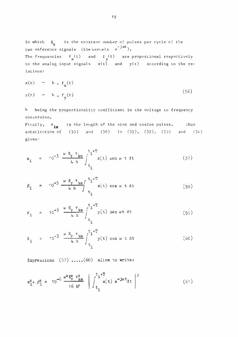
19

in which K is the constant number of pulses per cycle of the two reference signals (the kernels, e ). The frequencies f (t) and f (t) are proportional respectively -ι χ y to the analog input signals x(t) and y(t) according to the re­lations:

x(t) h . f (t)

y(t) = h . f (t) y (56)

h being the proportionality coefficient in the voltage to frequency conversion. Finally, τ, is the length of the sine and cosine pulses. Thus κβ substitution of (55) and (56) in (51), (52), (53) and (54) gives :

α. ι

ω Κ τ » ι 1 0 Ο 1—κβ_ j χ ^ s e n ω t d t

4 h t. ι

(57)

ω Κ τ, t.+T -5 ω τ kef x

10 -ΊΠΤ^Ι * (t) cos ω t dt

t. i (58)

t.+T , ω K τ Λ i 10-j) τ—Ke y(^t) s e n u t d t

4 h / t.

(5Í

δ. 1

t.+T ω K τ, r χ

10 ^ ]" / y(t) cos ω t dt

■'t.

i

(60)

Expressions (57) (6θ) allow to write:

aU β 10 ­6 τ ke

16 h2

t.+T χ ­jwt, x(t) e """dt

t. χ

(61)

20

¿τ^+δ2. = io ¿ ω3 Κ3 τ»

-6 τ ke 16 h3

t .+T ι

y ( t ) e'^åt (62)

. ω3ΐΡ τ 3

α .Γ .+ά .δ . = 10" b — — Re 1 1 1 1 16 h3

r - /· ι t^+T t .+T

(t)eJwtdt .ƒ X yCtJe-*»*«" ■'t.

χ t .

χ

(63)

α .δ . - f l . i r . χ χ " χ χ

¿ ω3Κ? τ? . - 6 τ ke τ 10 Im

16 h3

t .+T ι j o t .

t .+T X

( t ) e j a M - d t . y ( t ) e " j a ' l ' d t -jut.

(64)

I f we now remember t h e r e l a t i o n s ( 4 8 ) , (49) and ( 5 0 ) , we can see

t h a t i t i s p o s s i b l e t o o b t a i n the power s p e c t r a l d e n s i t y from the

q u a n t i t i e s a. , A. » i". and δ. :

Φ (u) = xx

1_11 2ττ k Τ

4 h3

l O ' V f ^ T ? K3

ke τ }>Μ> ■ h L· ίξ 2«i*i> χ=1 1=1

(65)

^ (ω) = yy

ι__±± 4 "h3 r -27 k τ ^ - 6 ^ ^ ^ ¿_(^+δ1) =

ke τ χ=1 1=1 (66)

Retf^O)) 1 1 1 4 h3 Έ~\ Ν 1 f 1 V? = 27 k Τ , ο ^ ^ j . ¿ ( a i W i } = 27 ta J ^ 1 * * 1 ^

ke τ i = 1 Γ ϊ = ϊ

(67)

Imtø (ju)) = 27 k T 1 0 - 6 ^ τ ^ ^ ^ α χ δ Γ β / χ ) = 2 7 ^ ^ ¿ « i V ^ r i=1

(68)

ke τ £Ξι

21

where power and cross-power spectral densities are expressed in volts squared per unit of angular frequency and, in agreement with their theo­retical definition, defined fot both positive and negative frequencies, 1 6 > .

If we want to express the spectral densities in squared volts per hertz, we have to multiply expressions (65) (68) by a factor 2ττ.

In the right-hand members of (65), (66), (67) and (68) du<

gnal analysis: we have introduced the normalization coefficient h for random si-

r

π f τ, Κ . _ - 5 — -

h ιο_3 ke_r_ (69)

r 2 h

and we have expressed the integration time Τ as:

τ = ? (7o:

since in the S.D.A. apparatus this time is defined, in the spectral analysis of random signals, as a multiple of the period 1/f of the frequency being examined ). The normalisation coefficient h depends upon the frequency decade under examination, but does not vary with the frequency, which means that τ, is inversely proportional to the frequency itself ). Its value is however supplied directly from the analyzer to the final computer, together with the quantities α. , β- y ^i ' δ. , the analysis frequency f , the n number of integration cycles, and the k number of repetitions ) ).

If the signals x(t) and y(t) represent respective­ly the excitation signal and the response of a linear system, it may be interesting to obtain the transfer function G(jw) of the system itself.

22

This can be obtained on the basis of the definition ) 16,

Gr(ju) Φ (ju) xy

Φ (u) XX

(71)

and by rearranging (65), (67) and (68); we have:

Re(G(j(j)) = Re Γ- Φ (ju)—\

xy -Φ (ω) J r

xx

Σ (

ν±+β

±*±:

1=1

~k (72)

1=1

Im(a(ju)) - Im

Φ (ω) _ xx

) (α.δ. - fl.ir.)

/ v

χ χ r

x χ' i=1

κ

^(«î*/^:

(73)

1=1

In fig. 1 is shown a brief sequential diagram of operation,

in which the operations performed by the computer, and those performed

by that part of the S.D.A. (indicated by the name "analyzer,,) which

processes the signals before the computer does, are listed separately

for clarity.

In Appendix A2, two computer programmes for power spectral

analysis of random signals are given in full, for cases where an Olivetti

P102 is employed as the final computer.

Analyzer Computer

Analysis

Read and ste

a . , fl. , ï . , 1 ι ' x '

re

δ. 1

1 Calculate

Cale :u l a t e

Σ («\ +

1 Σ Λ * 1 +

"V

δ',)

A

Cale :u l a t e x

v 1 1

+ fl. δ . )

A

Cai : u l a t e Σία.δ . Λ ι ι - fl.ir.) r 1 l y

i < k i = k

F i g . 1

Read and s to re f, k, η, h r

1 Calculate Φ (m ι

XX

A Calculate Ky{u)

1 Calculate *e(J (jv))

A Calculate Imf> ( j ω) j

A Calculate \^(ju)\

A Print res u l t s

24

2.) SPECTRAL ANALYSIS OF APERIODIC SIGNALS

Let x(t) and y(t) be two aperiodic signals; their

Fourier transforms are defined· ) as:

i (d«) 2π χ (t) e

-jut åt (74)

Y(j«) hf y ( t ) β - j « t

dt (75)

while the power and cross­power spectral densities can be obtained from

the following relations:

Φ (ω) xx

2ϊτ χ ( * > ) (76)

ífr (ω)

yy

2ττ Y(J«) (77)

* (Jw) = 2ττ l ( j « ) . Y(joj) (78)

The Fourier transforms (74) and (75) are complex conti­

nuous spectra and can be divided into amplitude density spectra (|x(jw)| >

|Y(j")|) and phase density spectra; it is clear that the amplitude den­

sity spectrum of a transient signal does not express the actual ampli­

tudes of the sinusoids composing the signal under examination (as they

are infinitesimal), but gives relative magnitudes only ) ).

Therefore, the energy spectra (76), (77) and (78) show

relative values; in fact the total energy (expressed in volt squared­

second) over an infinite range of frequencies is finite ), so that

the energy of each periodic component is an infinitesimal quantity.

25

2.1.) Fourier transform estimation

For the spectral analysis of aperiodic signals, one can

employ formulae of the type:

t +T

ï(ju) = ^ Γ x(t) e"Jwt dt (79)

* t o

where the error due to the finite analysis time becomes irrelevant if the

time T is chosen in such a way as to cover the whole period during

which the signal under examination has an amplitude too great to be igno­

red; such a time T is independent of the analysis frequencies, whe­

reas the instant t at which the analysis starts should be chosen

o J

appartunely during the transient in examination.

The real and imaginary parts of the Fourier transform of

x(t) and y(t) can then be estimated from the relations:

T

Re(X(jüj)) = ^ j x(t) cos ω t dt (80)

ι

Im(X(jcu)) = ­ ¿ j x(t) sen m t dt (81)

o

and from similar expressions for the signal y(t), having assumed the

instant t as the origin of the axis of the times, o

In expressions (80) and (81) measurement repetitions

are not indicated. In effect, even in the case of deterministic si­

gnals, such as the aperiodic signals, the averaging out of several mea­

surements is useful, insofar as it serves to reduce the influence of

spurious noise which sumperimposes itself upon the signal to be ana­

lyzed.

26

2.2.) Fourier transform estimation with the statistical dynamics analyzer

S.D.A.

The evaluation of the Fourier transforms of the aperiodic

signals x(t) and y(t) is performed, in the S.D.A. analyzer^

on the basis of relations:

Re(x(>)) = ­ti­ll. k 2ir

Γ

lì x(t) cos ω t dt

i=1

1 1 k 2ττ

Im(x( ju)) - - — "τ- ) / x(t) sen ω t dt

i=1

Re(Y(>)) = li­li k 2π

y(t) cos ω t dt

1*1

im(Y(>)) =­ττ­ y(t) sen ω t dt

_J χ

i=1

(82)

(83)

(84)

(85)

The data which the S.D.A. pre­processing system supplies to the ge­

neral purpose digital processor are α. , β ■ , X. and δ. v.'hich

χ ' r

x ' χ ι

(see formulae (57)...(60) ) can be expressed as:

α. χ

, u Κ τ _ 10·Ο 2_jœ 2 π Im(x(j(U))i

4 h (86)

27

"i 7 ω Κ τ.

10-3 I__ke_ 2π R e ^ ( j f t , ) ^ 4 h X

(87)

ir. X

10-3 " ** Tke 2π ΐΓη(γ(^)) 4 h (88)

, ω Κ τ. 10-3 I_ke_ 2π R e( Y ( j a J))_

4 h x (89)

where the subscript i indicates the ith of the k repetitions,

From the preceding formulae one obtains:

Re(x(jcu)) = i_ io3 _ > β r2 f τ, K k / Pi ke τ i=1

1 h k a —

i=

ß. (90)

Im(x(jo))) 10'

π f τ, K ke τ

i = 1

1

h k / ι a —

(91)

Re(Y(jW)) = *­10'

­2 f T

ke Kr

k

i=1

h.k ^δ1 (92)

Im(Y(j«)) = ­ % 10­

k

1 \— 2 ­ ■ ^ ^ " h l )

yi

* f τ, K k

/_ 1

ke τ i=1 i=1

(93)

28

where h , called the normalization coefficient for aperiodic signals, a represents the expression:

π2 f τ, Κ ke τ

h 10' (94)

whose value is supplied directly to the final computer from the matrix of the normalization coefficients; it depends upon the frequency decade under examination, but not upon the frequency itself.

In the case where x(t) and y(t) are respectively the input and the output of a linear, time - invariant system, their Fourier transforms also allow the determination of the system transfer function defined by:

&(>) Y(ja) X(jO))

(95)

Substitution of expressions (90) to (93) in (95) allows us to write: k

Re(&(jw)) = Re j(ju) L*(J«) J

i=1 (96)

*i i=1

Im(G(jo)) = Im Y(j->) X(J«)

1=1 (97)

1=1

Analyzer

i <k

Analysis

i = k

F i g . 2

Computer

Read and store

ai ' ^ i ' *i'

5i

i Calculate Σ α.

1 Calculate Σ fl,

i ^

i Calculate Σ ï .

i x

A Calculate Σ δ,

i

Γ

L Rea

f,

d and s tore

k, n, h a

1 Calcula

Calcula

te -Im(X(jw)j

1

te Re(x(joj)j

A

Calcula te -Im(Y(jw))

i

Calcula te Re(Y(jw);

A

P r i n t re s ul t s

30

In fig. 2 is given a brief sequential operating diagram for the Fourier analysis of aperiodic signals.

In Appendix A.3 the complete program for the Olivetti P102 computer is shown.

2.3.) Energy and cross-energy spectral density estimation

The energy spectral densities φ (ω) and φ (ω) xx yy

of the aperiodic signals x(t) and y(t) , and the cross-energy spectral density ψ (ju) can be calculated from (76) (77) and

xy (78), by using the estimated values of X(jw) and X(ju):

Φ (u) r x x x 2π Χ(άω) 2π

t +T o x ( t ) e - j w t dt (98)

Φ (u) yy

2TT Y ( > ) 1 2π

t +T - o y ( t ) e " J w t d t (59)

Φ ( ¿ω) xy

2π X(ju) . Y(ju)

t +T t +T

h i °^ eJwt dt

· ƒ y(t) e - ^ J t J t

d t

I t i s demonstrated ) t h a t :

(100)

lim Φ^ω) = V^u) T-» »

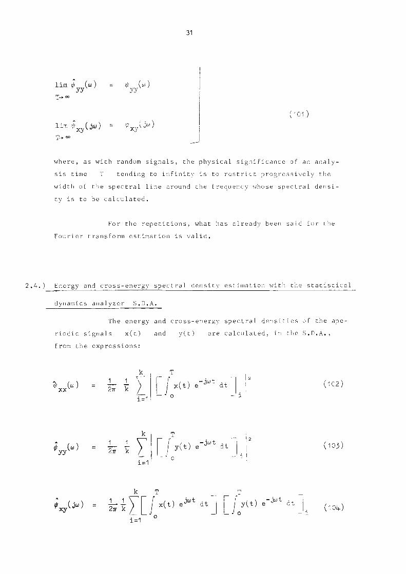
31

lim φ (u) yy

T->°°

li-n '>,;χνϋω;

í/r ( ω )

yy

Φ V ju xy

(^01)

where, as with random signals, the physical significance of an analy­

sis time Τ tending to infinity is to restrict progressively the

width of the spectral line around the frequency whose spectral densi­

ty is to be calculated.

For the repetitions, what has already been said for the

Fourier transform estimation is valid.

2.4.) Energy and cross­energy spectral density estimation with the statistical

dynamics analyzer S.D.A.

The energy and cross­energy spectral densities of the ape­

riodic signals x(t) and y(t) are calculated, in the S.D.A.,

from the expressions:

Φ (ω) xx

1_ 1 2π k

i=1

x(t) e"j W t

dt

— ι

(102)

Φ (u) yy

1_ 1 2TT k

i=1

y(t) e­Jwt dt (103)

k Τ

^xy(Jw) = h k x(t) e*"* dt

/ s -jUt j,

y(t) e cl t

i=1

(104)

32

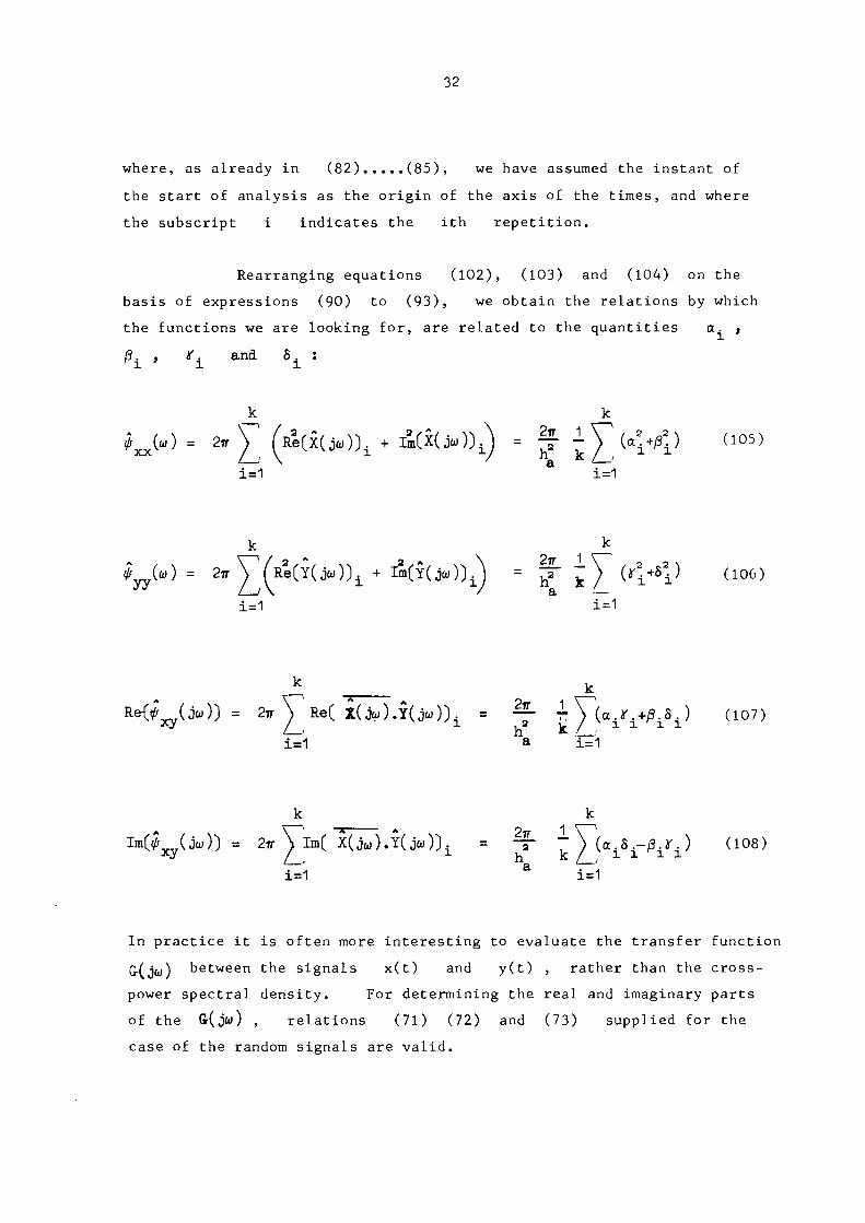
where, as already in (82) (85), we have assumed the instant of

the start of analysis as the origin of the axis of the times, and where

the subscript i indicates the ith repetition.

Rearranging equations (102), (103) and (104) on the

basis of expressions (90) to (93), we obtain the relations by which

the functions we are looking for, are related to the quantities α. ,

0. , ¿T. and δ. : r x ' ι χ

ft. K.

* „ ( « ) = 2 r £ V R I Ã J C O ) ) . + ImAja , )^ ) = f ± £ (α%Α2.) (105)

i=1 a i=1

k k

φ^(ω) = 2iryÍRe(Y(ju))í + ά(Υ(^ω))Λ = ψ ^ ) (*\+SV (106)

i=1 i=1

^ k Μφ (ju)) = 2ττ V R e ( l(ju).Y(ju)). = ^ r V(a.2r.+/3.8, ) (107)

^y /_, ι h k / . . 1 1 1 1

i=1 a i= i

Im( X(jo).Y(jw)). = - y - ) (α.δ,-fl.ar, ) (108) h k Z ^ 1 1 1 1

i=1 i=1

In practice it is often more interesting to evaluate the transfer function &(ju) between the signals x(t) and y(t) , rather than the cross-power spectral density. For determining the real and imaginary parts of the Gr(ju) , relations (71) (72) and (73) supplied for the case of the random signals are valid.

33

The sequence of operations in the S.D.A. system for the

energy spectral analysis of transient signals is in practise the same

as that for random signals, which can be seen in fig.l.

Appendix A4 presents in detail Lhe computation program­

mes for the Olivetti P102.

3.) SPECTRAL ANALYSIS OF PERIODIC SIGNALS

When one is dealing with periodic signals, the Fourier tran­

sforms of x(t) and y(t) are giver, by ).

Τ

X( jmw m Τ

x(t; e o (109)

t ­m­ü o 2

Is o 2

t + m ^

Y(jmuQ) m T

/, \ ­¿mu t ­y(t) e ° o at (110)

V - T

where T represents the period of the signal under examination,

and m the order of the analyzed harmonic, while t is an arbi­

o

trary value of the time chosen to be the central instant of the measu­

rement .

The functions X(jmOJ ) and Y(jmW ) are complex line

spectra. Their absolute values (i.e. the amplitude spectra") are

expressed in volts.

34

The power and cross-power spectral densities can be estimated from ):

φ (πιω ) XX o X(jmci» ) (111)

ti< (TOU ) yy o

Y(jw»0) (112)

ψ (jmcJo) = X(jmwo) . Y(jmwo) (113)

where, as already in (109) and (110), is the fundamental angular frequency of the periodic function to be analyzed.

The cross-power spectral density is a complex function; its absolute value and the power spectral densities are expressed in squared volts.

Expressions (109) (113) give, also for finite mea­surement times, determinations which correspond to the theoretical va­lues.

In practise it is better, as before in the case of aperio­dic signals, to repeat the measurement several times and to average out the results in order to reduce the influence of spurious noise which may have been superimposed upon the signal to be analyzed.

3.1.) Fourier transform estimation with the statistical dynamics analyzer S.D.A.

As we have already said, the Fourier transforms of perio­dic signals have line spectra; therefore the analysis is only carried out on the harmonics of the fundamental frequency of the expressions:

on the basis

35

Λ . t.+n m Τ

RefxUrn^)) = ^ \ j X °x(t) cos m % t dt

0 cJ h

(114)

ns;

k t.+n m T

ImfXUmw )) = ­ \ / x(t) ser. ­ i t ■ 0 k η m Τ / J

o ­ „ t

ι=ι r

i

and of the similar expressions for the signal y(t).

In equations (114) and (115) T and m repre­

' o '

sent respectively the period of the signal x(t) and the order of

the harmonic under examination, while η represents the number of

periods of integration and k the number of repetitions.

Taking equations (57) t<l (60) into a c c o u n t , and indica­

ting by ω' the angular frequency m u. and by T' the period

m Τ of the har m o n i c o f o r d e r m , the valu e s α Η ί o i I_ 2

ar.d o. supplied by the S.D.A. analyzer can be expressed in the fo 1 lowing way :

a . ι

' i

, ω1 τ, Κ ]Q-) ice τ η T' Im(X(jaj')

4 h ιΝ ( 1 IM

ω' τ Κ ΙΟ*·5 — — — η Τ' Rel'XÍJt« )"; ( 1 1 7)

4 h

ω' τ, Κ

ï. = - 10­J>

ke_r_ η τ, I m r v ( > t y ι 4 h

, ω' τ. Κ

¡Ο­"5 K e Τ

η Τ' Re(Y(>')'

(1 IS ')

(11 c> )

4 h

because of which, in the case of k repetitions, the real and imaginar)

36

parts of the Fourier transforms of the periodic signals x(t) and

y(t) are given by:

3 k k

Re(x(ju')) = ¿ ? , 1 0 , £ V f l . = Τ-^ττΥ ß ( 1 2 0 )

k π n r k e Kr /_fx k n h p ¿ P i

1=1 i=1

1

k

2 . 1 0 3 . h

π n τ . K ke τ

k

1=1

k

f' v^ k n h /

Ρ l— 1=1

im(x( j" ' ) ) = - r Γ ^ Γ Τ — — > », = - r — — > ^ (121)

H.CÎO·» - è ^ # V V 8 , - r£ rV.< k π n τ, K / i k n h

ke τ ƒ__ ρ / i=1 1=1

k ,*, .N-, 1 2 Ί 0 » h \~^ fi

Im(Y(^· ) ) = - £ , n T t o Kr ¿ , / i = - T h r ) * i ( 1 2 3 )

1=1 P fel

where h represents the normalization coefficient for the spectral

Ρ analysis of periodic signals, and is given by:

" Tke Kr 'f ' h = SL­I (124)

P 2 10

5 h

where the product Τ · f' is independent of the frequency.

Κ. θ

As far as the determination is concerned, through the Fourier

transforms, of the transfer function of the system in which x(t) and

y(t) are respectively the input and the output signal, the relations

(96) and (97) are valid.

37

In Appendix A5 the programmes (for Olivetti Ρ 102) relative to the Fourier analysis of periodic signals are shown.

3.2.) Power and cross-power spectral density estimation with the statistical dynamics analyzer S.D.A.

The power spectral densities φ (ω j and ύ (ω) of xx yy

the periodic signals x(t) and y(t) , and their cross-power spec­tral density φ ( j w ) are calculated, in the S.D.A. svstem, by

xy J

virtue of the relations:

xx o k 2 2ma n m Τ

t.+η m Τ ι o *χχ(™ο> = Ï T T L T ") !/ x ( t ) e ­ ^ o

t o dt i (125)

o h­, \J t.

1=1 i

t.+n m Τ χ o

φ (w ) = i —J V / y(t) e

_ >V dt

yy o k

n m2

T2

(126)

o '—, 't. x=1 χ

k t.+n m T t.+n m Τ

η' πΤ Τ"

χ ο 1 1 \ / f,\ +jmit

*»<» = Ϊ Τ Ζ ; / x(t)e-^Vdt y(t) e"*»,,* dt 1 o

0 Γ-1 t, t. 1=1 ι 1

(127)

where k , η , m , Τ and t. have the same meaning as in equations (114) and (115).

By taking equations (120) to (123) into account, we have :

38

Φ (u>) rxx

1 k

Ψ .(ω')

1=1

k

•12

n 2 h

3 (4^1) 1=1

(128)

Φ (ω') yy

k Φ .(u') vyy,i

i=1

k

fl2

n3 h

2

Ρ 1=1

(*!**!) (129)

k

i=1 Ρ i=i

(130)

k

lm(¿xy(̂ »)) = ¿ yim(íxy)i(>·)) = 1-fj 7 ( - δ Γ ^ ί ) (131) 1=1

n2 h2 /-Ρ 1=1

For the determination of transfer functions from power spectra, relations (71) (72) and (73) , given for random si­gnals, are valid.

Appendix A6 gives the programmes for the determinations set out above.

39

A P P E N D I X

A.l.

Computing programmes for the computer composing the final element of the S.D.A. system all have a common structure, irrespec­tive of the type of analysis to which they refer.

A typical programme can in fact be considered to be compo­sed of four parts.

The first part (from AZ to AV , if an Olivetti Ρ 102 is being used) corresponds to the introduction of data α χ

and δ. , into the machine, and, when the repetitions are finished, of the values f, n, k and h , where the generic normalization

n coefficient is indicated bv h

n The second part of the programme (AV Z) processes

the data in order to obtain the functions for which one is looking.

The third part, (AW Z) is designed to carrv out a nor­malization of the quantities calculated in the second part, and to print the results.

The final part of the programme performs the sequence of ope­rations linked to an overload of the S.D.A. system. Any type of overload (for exemple in the input amplifier, or in the α , β , Χ , δ , counters) in fact cancels out the number of the repetitions , which number, in normal operating conditions, is never zero. The cancella­tion of k triggers off this part of the programme ( /V ), which interrupts the calculation sequence relative to the point under examina­tion, cancels any results relative to it which have already been obtained, and takes the apparatus forward to the following point.

Finally, a practical consideration is made. For any kind of processing (e-g. spectral analysis of random signals), and by using

40

the data α. , β. , ¿% , δ. , f , η , k an¿¡ h ι χ ι χ η

supplied by the analyzer to the final computer, it would be possible to

calculate all the interesting functions in one programme, if only the

capacity of the computer did not place limits upon the length of program­

me that can be memorized.

We therefore list here, for each function of the S.D.A. ,

different programmes, each one of which calculates some of the functions

of interest. The programmes are written for the Olivetti Ρ 102.

41

Α.2. ­ Programmes for the power spectral analysis of random signals

Table A.2.1. describes the programme which calculates

the power spectral densities φ (ω) and φ (ω) of the random

xx yy

signals x(t) and y(t) being dealt with.

Results will be printed in the following order:

f

k

in Hz

φ (ω) in V^/HZ

(analysis frequency)

(repetition number)

(number of integration ciclos

xx

φ (ω) in ν2 /Hz yy

Table A.2.2. shows the programme for calculating the

power spectral density of the signal x(t) , and the real and

imaginary parts and the modulus of the cross­poxver spectral density

^xy(¿w) ·

Results will be printed in the following order:

f in Hz

k

n

^ χ χ(ω) in ν2/Hz

Re(í (¿ω)) in ν2/Hz

Imí<Â (ju)) in ν2/Hz

" xv

\φ (ju)\ in ν2 Hz

|Txy'

42

Table Α.2.3. shows the programme concerned with the

calculation of the transfer function G­(jtø) of the system of

which x(t) and y(t) represent respectively the input and the

output signal.

Results will be printed in the following order:

f in Hz

k

n

Re(&(jw))

Im(G(jo)))

Im(&0)) tgp =

Re(&(jo)))

This last programme is the same also for periodic and aperiodic signals,

since for the calculation· of the &(j(u) one uses power spectra ra­

tios in which there are no normalizations.

In effect, the values of the power and cross­power spec­

tral densities are half of the real values, because they are supplied

as bilateral spectra (i.e. also for negative frequencies).

The transfer function is calculated as a ratio of spectra and is there­

fore in effective values.

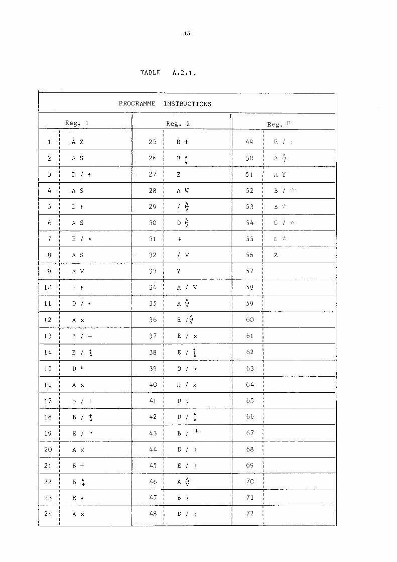
43

TABLE Α . 2 . 1 .

PROGRAMME INSTRUCTIONS

Reg. 1

1 ! Α Ζ

2 ! A S

3 ! D / t

4 ! A S

5 1 Dt

6 ! A S

7 ! E / t

8 ! A S

9 ! A V

IO ! E t

1 1 1 D / +

12 ! Α χ

1 3 ! Β / +■

14 | Β /. \

15 ! D +

16 ! Α χ

17 ! Β / +

18 ! Β / χ

19 ! Ε / ;

20 ! Α χ

21 ! Β +

22 ! Β \

23 ! Ε Ι

24 ! Α χ

Reg. 2

25 ! Β +

26 | Β J

27 ! Ζ

28 ! A W

29 ! / $

30 ! D φ

31 ¡ 4·

32 ¡ / V

33 ,' Υ

34 1 Α / V

Reg. F

49

50

51

52

53

i 54

55

56 ■

! 57 I

58

35 ! A Ô 59 1

36 Ε /Ο 60

37 ¡ Ε / χ 61

38 Ι Ε / \

39 ! D / 4.

40 ¡ D / χ

41 ! D :

42 D / I

43 ! Β / i

44 ! D / :

45 ! E / :

46 ! Α φ

47 ! Β +

ι

48 ! D / :

62

63

64

65

66

67

68

69

70

71

72

1

E / :

Λ

A y

A Y

Β / *

Β -'■-

c / --'-

c ··-

Ζ

44

TABLE Α . 2 . 2 .

PROGRAMME INSTRUCTIONS

Reg. 1

ι !

2 !

3 !

4 !

5 !

6 !

7 !

8

9

10

11

12

13

14

15

16

17

18

19

20

21

.22

23

24

A Ζ

A S

D / t

A S

D t

A S

E / t

A S

A V

E t

D / 1

A χ

B / +

B / J

D V

A χ

Β / +

Β / |

D / 1

! Ε / χ

! c / +

! c ' 1 D 4

Ι Ε χ

Reg. 2

25 j C / +

26 ; C / J

27 '¡ D i

28 ¡' E / χ

29 ¡ D / J

30 E x

31 j D / ­

32 C +

33 i

c ι

34 j Ζ

35 j AW

36 ; / ν

37 j D φ

38 j *

39 j / V

40 j Y

41 A / V

42 j A 0

43 j E / φ

44 ! E / χ

45 j D / J

46 Α χ

47 ; D :

48 j Β / J

Reg. F

49 j

50 ';

51 j

52

53

54 j

55 |

56

57

58

59

60

61

62

63

64

65

66

67

68

69

70

71

72

Β / :

D / :

A v

C / *

B / :

D / :

A v

A χ

C t

B / :

D / :

AO

A χ

C +

Α -r

AO

A Y

B / *

B *

C / *

¡ C *

! z

45

TABLE Α . 2 . 3 .

PROGRAMME INSTRUCTIONS

Reg. 1

1

2

3

4

5

b

7

8

9

10

1 1

12

13

14

15

16

17

18

19

20

21

22

23

24

A Ζ

A S

D / t

A S

D ,

A S

E / .

A S

A V

E t

D / +

A χ

B / +

B / I

D *

A χ

Β / +

Β / 1

D / 4

Ε / χ

C / +

c / Χ

D 4.

Ε χ

Reg. 2 jj

25 ! C / +

26 ! C / I

27 ! D 4

I ! 28 . E / χ

29 ! D / I

; 30 ! E x

31 Ι D / ­

! J I 32 ι C +

! 33 ! C \

¡ 34 ! Ζ

35 I A W

36 i / O !

37 ! D {? !

38 ! 4

39 ! / V

40 ! Y

41 ! A / V

42 ! A V

1 ! ; 43 ι E / v

44 ! C / 4

45 i B / :

46 ¡ A 0 1

47 ι A x

48 ! E / %

49

i 50

i

51

1

! 5 2

i 5 3

54

i 55

i 56

57

58

59

60

61

62

' 63

64

65

66

67

68

69

70

71

72

Reg. F

C ­

B / :

Av*

A χ

E / ­

A .Γ

A 0

C v

C / :

A "

Λ Y

B / ■;·■­

B ··'■­

c / ­■'■­

c ·'-

Ζ

46

A.3. ­ Programme for computation of the Fourier transforms of aperiodic

signals

Table A.3.1. shows the programme which calculates

the real and imaginary parts of the Fourier transforms X(jw)

and Y(ja) of the two aperiodic signals x(t) and y(t).

Results will be printed in the following order:

f in Hz

k

Τ in sec. ( analysis time )

Im(x(jaO)

Re(X(jû)))

Im(Y(>))

Re(Y(jü)))

47

TABLE A . 3 . 1 .

PROGRAMME INSTRUCTIONS

Reg. 1

1 |

2 ;

3 |

4 |

5 j

6

7

8

9

10

11

12

13

14

15

16

17

18

19

20

21

22

23

24

A Ζ

A S

D / t

A S

D t

A S

E / t

A S

A V

4

C +

c I

R e g . 2

1 li

25 ; D '0 i!

26 ! * ;

27 ; /V

í 28 ; Y

! t

29 ,' A / V

3 o ; A A !

31 ¡ D / χ

ii 3 2 ¡ D t ti i

1

' 33 ¡ A / t

¡i ' i ii 1 i

!: 34 ¡ R *

i ι

; 35 ¡ R S

ti ' i

36 ; D / s

Il ι

D / 4

B / +

B / I

D 4

B +

B Î

! E / *

C / +

i c / X

! z

; A w

i ή

3 7 ; 4 ;

38 ; E / χ

39 ', Α 0

40 | Β / 4

41 ; D :

42 ', Α χ

43 ; Β 4

44 j D :

45 ; A y

46 ; C / 4

47 ; D :

48 ; A 0

1

49

50

51

52

53

54

55

5b

5 7

58

59

60

61

62

b3

64

65 ι

66

! 6 7

68

; b«

70

71

|! 72 1 II

}eg. F

c -

D :

A ^

A Y

B / *

B --'■-

C / *

C ,

Ζ

48

Α.4. - Programmes for the energy spectral analysis of aperiodic signals

In Table A.4.1. we list the programme for calculating the energy spectral densities φ (u) and ψ (u ) of the tran-

xx yy sient signals x(t) and y(t).

The results obtained by the programme are:

f in Hz

k

Τ in sec (analysis time)

φ (u) in volt squar-ed-second per hertz

Φ (ω) yy

π n it η ii it

Table A.4.2. shows a programme which evaluates the energy spectral density ψ (ω) and the real part, the imaginary part and the modulus of the cross-energy spectral density φ (ju).

xy The following quantities will be printed out as computing

results:

f in Hz

k

Τ in sec. φ (ω) in volt squared-second per hertz xxv

ImQ (ju))

4S

TABLE Α . 4 . 1 .

PROGRAMME INSTRUCTIONS

Reg. 1

1 ! Α Ζ

2 j A S

3 j D / t

4 ! A S

5 ; D t

6 ί A S

7 E / t

8 ! A S

9 i A V

IO ! E f

11 ¡ D / φ

12 1 Α χ

13 ! Β / +

14 | Β / Ι

15 i D 4

16 ! Α χ

17 j Β / +

18 j Β / i

19 ! E / 4

20 ! A χ

21 j Β +

22 ί Β î

23 ί E 4

24 ! Α χ

Reg. 2

25 j Β +

26 j Β î 27 j Z

28 ¡ A W

29 j / 0

30 j D Ø

31 j *

32 j / V

33 j Y

34 ! A / V

35 j A 0

36 ! D / χ

37 ! D / χ

38 ί Ό / Ι

39 | Α / t

40 ! R 4

41 j R S

42 j D / S

43 j 4

44 j E / χ

45 j A 0 46 j Β / ;

47 j D / :

48 i A 0 1 I

Reg. F

49 ! Β *

50 ί D / :

51 ! AV

52 ¡ A Y

53 | B / *

54 j B *

55 j C / ­'­­

56 j C ­­'■­

57 j Z

58 j

59 j

60 !

61 |

62 j

63 |

64 j

65 |

66 ¡

67 j

68 |

69 |

7 0 !

71 |

72 ¡

50

TABLE Α . 4 . 2 .

PROGRAMME INTRODUCTIONS

Reg. 1

1 ! Α Ζ

2 ! A S

3 ! D / *

4 ! A S

5 ! D t

6 ! A S

7 ! E / t

8 ! A S

9 ! A V

10 ! E *

11 ! D / ^

12 ! A x

13 ! B / +

14 ! B / t

15 ! D 4

16 ! A χ

17 ! B / +

18 ! B / l

19 ! D / +

20 ! E / χ

21 C / +

22 ! C / t

23 ! D 4

24 Ί E x

Reg. 2

25 ! C / +

26 ! C / t

27 ! D *

28 ! E / χ

29 D / ♦

30 ! E x

31 D / -

32 ! C +

33 C J

34 Ζ

35 ! AW

36 ! / $

37 DV

38 ! +

39 ! / V

40 ! Y

41 ! A / V

42 A 0

43 D / χ

44 D / χ

45 D / χ

46 A / t

47 R *

48 ! R S

Reg. F

49 ! D / S

50 j *

51 ! E / χ

52 j A 0

53 ! Β / +

54 D / :

55 ; A O

56 ! C / 4

57 D / :

58 A 0

59 ! Α χ

60 C J

61 ! D / :

62 ! A 0

63 A x

64 C +

65 ΑχΛ

66 A 0

67 ¡ A Y

68 Β / *

69 Β *

70 C / *

71 C *

72 Ζ

51

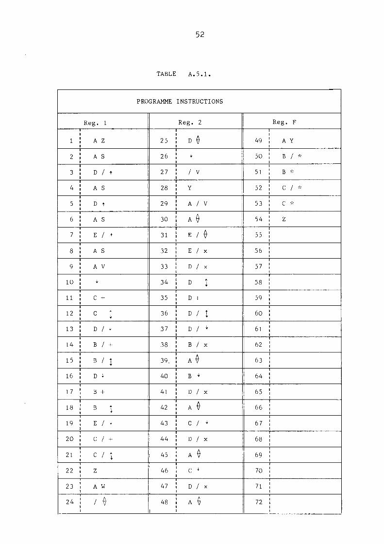
Α.5. - Programme for computation of the Fourier transforms of periodic

signals

In Table A.5.1. we show the programme which calculates

the real and imaginary parts of the Fourier transforms X(jw) and

Y( V J ) of two periodic signals x(t) and y(t) .

Results will be printed in the following order:

f in Hz

k

Im(X(ju);

ReíX(jüj))

In/Y(jo>)j

Re(Y(>))

52

TABLE Α . 5 . 1 .

PROGRAMME INSTRUCTIONS

Reg. 1

1 ! A Z

2 ! A S

3 ! D / t

4 ! A S

5 ¡ D t

6 ! A S

7 ! E / t

8 ! A S

9 ! A V

IO ! 4

ii ! c +

i2 c ;

13 ! D / »

14 ¡ B / +

15 j B / I

16 ', D 4

17 ! Β +

18 j Β ♦

19 I E / .

20 ! C / +

21 C / I

22 ¡ Ζ

23 ! A W

24 j / A

Reg. 2

25 : D ^

26 ¡ 4

27 ! /V

28 ¡ Y

29 ¡ A / V

30 A 0

31 ! E / 0

32 ! E / χ

33 i D / χ

34 ! D I

35 ! D :

36 ¡ D / I

37 ¡ D / ;

38 Β / χ

39. ! A 0

40 ¡ Β 4

41 ! D / χ

42 A 0

43 ! C / 4

44 ¡ D / χ

45 ! A 0

46 C 4

47 ! D / χ

48 ! A 0

Reg. F

49 ! A Y

5o ; Β / *

51 Β *

52 ! C / *

53 ! C *

54 ; Ζ

55 !

56 !

57 !

58 ¡

59 !

60 !

61 ;

62 ¡

63

64 !

65 !

66

67 !

68 !

69 I

70

71

72 !

53

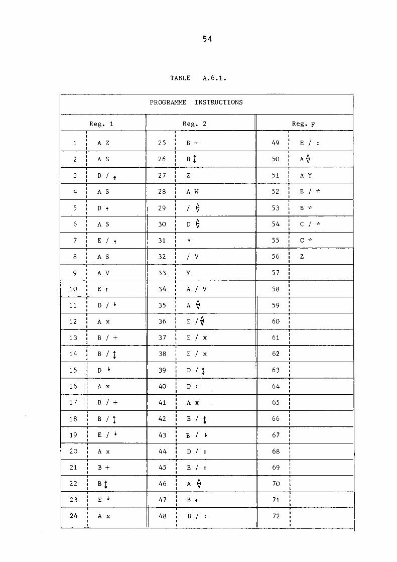
Α.6. ­ Programmes for the power spectral analysis of periodic signals

Table A.b.l. shows the programme for calculation of

the power spectral densities φ (ω) and φ (ω) of the periodic

xxK yy

v

signals x(t) and y(t) under examination.

The following quantities will be printed as computing re­

sults, at every analysis frequency:

in Hz

(ω, xx

Φ (u )

yy

Table A.6.2. shows the programme which deals with the

calculation of the power spectral densi tv oí the signal x(t) and

of the real part, the imaginary part and Lhe modulus of the cross­power

spectral density of the signals x(t) and y(t).

Results will be printed in the following order:

f in ¡lz

k

φ (ω) xx

Re(¿xy(>))

ImO ( ja))

kXy(ja)|

As far as the calculation (starting from φ (u) and ψ (ju) )

χχκ xy

of the transfer function between the signal x(t) and y(t) is

concerned, the programme written for random signals, shown in Table

A.2.3. , r ema ins valid.

54

TABLE Α . 6 . 1 ,

PROGRAMME INSTRUCTIONS

Reg. 1

1 ! Α Ζ

2 ! A S

3 | D / t

4 ! A S

5 ! D t

6 1 A S

7 ; E / t

8 ! A S

9 ! A V

IO ! E t

11 ! D / 4

12 ! A χ

13 ! Β / +

14 ! Β / |

15 ! D 4

16 ! Α χ

17 ! Β / +

18 Β / Ι

19 ! Ε / 4

20 ! Α χ

21 ! Β +

22 ! Β J

23 ! Ε *

24 ! Α χ

Reg. 2

25 Ι Β +

26 ! Β Ι

27 ¡ Ζ

28 ! A W

29 ! / 0

30 ! D f}

31 4

32 ! / V

33 ! Y

34 A / V

35 ! A 0

36 ! E /$

37 ! E / χ

38 E / χ

39 D / χ

40 D :

41 ! Α χ

42 ! E / I

43 Β / 4

44 ! D / :

45 E / :

46 A 0

47 ! Β 4

48 ! D / :

!

Reg. F

49 E / :

50 A4)

51 ! A Y

52 Β / *

53 Β *

54 C / *

55 C *

56 Ζ

57

58

59

60 !

61

62

63 !

64 !

65

66 !

67

68

69

70

71

72 !

!

55

TABLE Α . 6 . 2 ,

PROGRAMME INTRODUCTIONS

Reg. 1

1 ; Α Ζ

2 ¡ A S 1

3 ί D / t

4 ¡ A S

5 j Dt

6 ¡ A S

7 ! E / t

8 ; A S

9 ¡ A V

IO ! Et

!

11 ¡ D / 4

12 ¡ A x

13 ¡ B / +

i4 ; B / l

¡ 15 ; D 4

16 ¡ Α χ

17 j Β / +

18 ¡ Β / I

19 j D / 4

20 ¡ E / χ

21 ¡ C / +

22 ¡ C / I

23 ! D 4

24 ¡ E x

Reg. 2

25 j C / +

26 ¡ C / I

27 j D 4

28 ¡ E / χ

29 j D / I

30 ¡ Ε χ

31 ¡ D / ­

32 ; C +·

33 ; c ι

34 ; Ζ

I 35 ! A W

36 j / ν

37 j D f)

38 j *

39 ; / V

I 40 ; γ

I !

4i ; A / V

42 j A 0

43 j E /f)

44 ¡ E / χ ί ι Ι ,

45 ; Ε / χ 46 j D / %

47 j D :

48 ¡ Α χ

Reg. F

49 j Β / t

50 \ Β / :

51 | D / :

52 | Α {;

53 ¡ C / 4

54 \ Β / :

55 j D / :

56 ¡ A 7

57 ! Α χ

58 j C ;

59 ; B / :

60 ¡ D / :

61 ! A V

62 ; A χ

63 ¡ C ­

64 ¡ A -.Γ

65 j A v ι

66 ¡ A Y

67 j Β / *

68 ; Β *

69 J C / *

70 ¡ C *

71 j Ζ

72 j

FIGURE CAPTIONS

56

Fig. 1 Power spectral analysis of random signals: sequential diagram of operation of the S.D.A. system.

Fig. 2 Estimation of the Fourier transforms of aperiodic si­gnals: sequential diagram of operation of the S.D.A. sy s t em.

LIST OF TABLES

Table A.2.1. Programme for calculating the power spectral densities of random signals.

Table A.2.2. Programme for calculating the power and cross-power spec­tral densities of random signals.

Table A.2.3. Programme for evaluating the transfer function on the basis of power and cross-power spectral densities.

Table A.3.1. Programme for the estimation of the Fourier transforms of aperiodic signals.

Table A.4.1. Programme for calculating the energy spectral densities of aperiodic signals.

Table A.4.2. Programme for calculating the energy and cross-energy spectral densities of aperiodic signals.

Table A.5.1. Programme for estimating the Fourier transforms of perio­dic signals.

Table A.6.1. Programme for the calculation of the power spectral den­sities of periodic signals.

Table A.6.2. Programme for calculating the power and cross-power spec­tral densities of periodic signals.

£., 7

KEFKKKNCES

. ) " I d c n l i l ¡ f a t i o u ¡π a u t o m a t i c c o n t r o l s y s t e m s "

P r o c e e d i ug "f '-h'· I FAO S y m p o s i u m , P r a g u e , 1 2 - 1 7 June 1 9 6 7 .

2 ".) li.HARRIS ­ "Speri ral analysis of time series"

John Wiley, (1967).

.) .I.A.TUIE ­ "Reactor Noise"

Rowrnan and Littlefield, ("1963).

4

.) l.BMDAEL ­ A.GARRONI ­ A.LUCIA ­ F.SCIUTO ­ "Design and operating charac­

teristics of an equipment for identification"

Proceeding of X Automation and Instrumentation Congress, Milan, 20­26

Nov. 19 68.

.) V.V.S0L0D0VNIK0V ­ "Statistical dynamics of linear automatic control

systems"

D. Van Nostrand (1965).

.) M.S.UBEROI ­ E.G.GILBERT ­ "Technique for measurement of cross­spectral

density of two random functions"

The Review of Scientific Instrument ­ Vol.30, n.3, March 1959.

.) A.GARRONI ­ "Considerazioni su un metodo spettrale diretto per l'identi­

ficazione dei sistemi lineari"

Report EUR 3734 i (1968).

o

.) W.B.DACENPORT ­ W.L.R00T ­ "An introduction to the theory of random signals

and noise"

Mc Graw Hill Book Co. (lü58).

9 .) V.S.PUGACHEV ­ "Theory of random functions"

Ρ e r gamo η 1' r ess ( 1 ^ b 5 Ί.

58

.) J.H.LANING - R.H.BATTIN - "Random processes in automatic control" Mc Grw Hill Book Co. (1956).

.) J.L.DOOB - "Stochastic processes" John Wiley (1953).

1 2 .) H.CRAMER - "Mathematical methods of statistics"

Princeton Univ. Press. (1958).

.) A.M.MOOD - F.A.GRAYBILL - "Introduction to the theory of statistics' Mc Graw Hill Book Co. (1963).

1 4 .) R.B.BLACKMAN - J.W.TUKEY - "The measurement of power spectra"

Dover Publications (1958).

.) A.LUCIA - F.SCIUTO - "Operating manual of the statistical dynamics analyzer S.D.A. - Mod. 040". To be published.

.) J.W.LEE - "Statistical theory of communication" John Wiley (1964).

.) A.GARRONI - A.LUCIA - "Identificazione di sistemi controreazionati mediante rilievi della matrice spettrale" Report EUR 4458(1970).

1 8 .) A.PAPOULIS - "The Fourier integral and its applications"

Mc Graw Hill Book Co. (1962).

Tf' JSla "a

NOTICE TO T H E READER

fii tø .«'ηρΙ,Ι* iLC] AU Euratom reports are announced, as and when they are issued, in the monthly periodical " euro abstracts ", edited by the Centre for Information and Documentation (CID). For subscription (1 year : <£. 6.17, US$ 16.40) or free specimen copies please write to :

PP m>$W

Handelsblatt GmbH

" euro abstracts "

Postfach 1102

D 4 Düsseldorf 1 (Germany)

■ ■ ■■

or

m- mkw Office de vente des publications officielles

des Communautés européennes

37, rue Glesener

Luxembourg

«I» MRS

st.

. , ,

To disseminate knowledge is to disseminate prosperity — I mean

general prosperity and not individual riches — and with prosperity

disappears the greater par t of the evil which is our heritage from

! darker times.

■

Alfred Nobel

filini·

If t&bfciii

κ

iii

ifitML'î.llf ■iti I ;F .: B íWl" J ι'η*-s

ι reports published by the Commission of the European Communities are on sale at the offices listed below, at the prices given on the back of the front cover. When ordering, specify clearly the EUR number and the title of the report which are shown on the front cover.

mw

ma: «13£

!

SALES OFFICE FOR OFFICIAL PUBLICATIONS OF THE EUROPEAN COMMUNITIES

iSIllii

1

mm- ^ mmämwå BELGIQUE - BELGIË

MONITEUR BELGE Rue de Louvain 40-42 - 1000 Bruxelles BELGISCH STAATSBLAD Leuvense weg 40-42 - 1000 Brussel

LUXEMBOURG ÌUkM R;

OFFICE DE VENTE DES PUBLICATIONS OFFICIELLES DES COMMUNAUTES EUROPENNES 37, nie Glesener - Luxembourg

DEUTSCHLAND

BUNDESANZEIGER Postfach - 5000 Köln 1

FRANCE

f'Tí y 'ìtF

1

fÊBmm SERVICE DE VENTE EN FRANCE DES PUBLICATIONS DES COMMUNAUTES EUROPEENNES 26. rue Desaix - 75 Paris 15°

NEDERLAND

STAATSDRUKKERIJ Christoffel Plantijnsiraat - Den Haaf

ITALIA

LIBRERIA DELLO STATO Piazza G. Verdi, 10 - 00198 Roma

UNITED KINGDOM

H. M. STATIONERY OFFICE

lip. RO· Box 569 -London S E · ·

¡.feii!!ÉP!^ β

•I*!·..«

Commission of the European Communities

ïÜliiSi

D.G. XIII - C.I.D. 29, rue Aldringer L u x e m b o u r g

CDNA04479ENC W H