arX

iv:1

803.

0812

7v2

[m

ath-

ph]

10

Apr

201

8

SPECTRAL STATISTICS OF NON-HERMITIAN RANDOM MATRIXENSEMBLES

RYAN C. CHEN, YUJIN H. KIM, JARED D. LICHTMAN, STEVEN J. MILLER,SHANNON SWEITZER, AND ERIC WINSOR

Abstract. Recently Burkhardt et. al. introduced the k-checkerboard random matrixensembles, which have a split limiting behavior of the eigenvalues (in the limit all but k of

the eigenvalues are on the order of√N and converge to semi-circular behavior, with the

remaining k of size N and converging to hollow Gaussian ensembles). We generalize theirwork to consider non-Hermitian ensembles with complex eigenvalues; instead of a blip newbehavior is seen, ranging from multiple satellites to annular rings. These results are basedon moment method techniques adapted to the complex plane as well as analysis of singularvalues.

Contents

1. Introduction 21.1. Background 21.2. Results 32. Complex checkerboard ensembles 102.1. Singular values of complex checkerboard matrices: bulk 102.2. Singular values of complex checkerboard matrices: blip 132.3. Eigenvalues of complex checkerboard matrices: bulk 153. Generalized checkerboard ensembles 233.1. Analogs of bulk and blip results for generalized checkerboard ensembles 233.2. Eigenvalues of complex checkerboard matrices: blip 243.3. Conjectures 27Appendix A. 27A.1. Notation and terminology for cyclic products 27A.2. Joint density for singular values of complex symmetric Gaussian ensemble 29References 32

Date: April 11, 2018.2010 Mathematics Subject Classification. 15B52 (primary), 15B57 (secondary).Key words and phrases. Random Matrix Ensembles, Singular Values, Checkerboard Matrices, Limiting

Spectral Measure, Split Limiting Behavior, Joint Density.The authors were partially supported by NSF Grants DMS1561945, DMS1659037, the University of

Michigan, Princeton University, and Williams College. We thank Arup Bose, Peter Forrester, Roger vanPeski, and our colleagues from SMALL 2017 for helpful conversations.

1

1. Introduction

1.1. Background. Random matrix ensembles have been studied for almost a hundred years.The eigenvalues of these ensembles model many important and interesting behavior, fromthe waiting time of events to the energy levels of heavy nuclei to zeros of L-functions innumber theory; see for example the surveys [Bai, BFMT-B, Con, FM, KaSa, KeSn] and thetextbooks [Fo, Me, MT-B, Tao2].There are many questions one can ask about these eigenvalues. This paper is a sequel to

[B–]. There, in the spirit of numerous previous works, the authors investigated the densityof eigenvalues of some highly structured ensembles. One of the central results in the subjectis due to Wigner [Wig1, Wig2, Wig3, Wig4, Wig5], which states that the distribution ofthe scaled eigenvalues of a typical real symmetric matrix converges, in some sense, to thesemi-circle distribution. However, if the real symmetric matrices have additional structurethen other distributions can arise; see for example [Bai, BasBo1, BasBo2, BanBo, BLMST,BCG, BHS1, BHS2, BM, BDJ, GKMN, HM, JMRR, JMP, Kar, KKMSX, LW, MMS, MNS,MSTW, McK, Me, Sch].In all those examples the limiting distribution has just one component. Different behavior

is seen in the limit as N → ∞ of the k-checkerboard N × N matrix ensembles of [B–] (seealso [CDF, CDF2]), described later in Definition 1.1. There, all but k of the normalizedeigenvalues converge to a semi-circle centered at the origin; however, there are k eigenvalueswhich diverge to infinity together. Further, these k blip eigenvalues converge to a universaldistribution, the k-hollow GOE distribution (obtained by setting the diagonal of the k × kGOE ensemble to 0).Below we describe the ensembles studied in [B–] and discuss our generalization (see Def-

initions 1.8 and 1.10). In particular, we find ensembles where there can be multiple blipsor satellites orbiting the bulk of the eigenvalues, as well as a ring of eigenvalues around thecentral mass; Figure 1.

Figure 1. Two numerical examples of distributions which can arise from ageneralized k-checkerboard ensemble. Left: A collection of satellites. Right:A ring of eigenvalues.

2

In the next subsections we define the ensembles we investigate and state our results.Unfortunately many of the techniques used for related ensembles are not applicable here,and thus we spend some time describing the needed tools and approach.

1.2. Results. Random matrix ensembles with real entries see markedly different behaviorbetween asymmetric and symmetric entry choices – for example, the symmetric ensemblesare Hermitian with real eigenvalues, and this need not hold for asymmetric ensembles. Al-lowing matrices with complex entries, we also find differences between the asymmetric andsymmetric (not-necessarily Hermitian) ensembles in the joint density formulas.Recall that the joint density function for singular values returns the probability that any

given matrix has a certain N -tuple as its singular values.SupposeM is a random N×N matrix (for example, real asymmetric, complex symmetric,

etc.). The joint density function ρN for the singular values satisfies∫

RN≥0

F (x1, . . . , xN )ρN(x1, . . . , xN) dx = E

∑

σ21,...,σ2

N∈λ(M∗M)

F (σ1, . . . , σN) (1.1)

for any test function F , where the right-hand sum is interpreted as over all N ! orderings ofthe N eigenvalues of M∗M (and the σj are nonnegative).We list the available singular value joint density functions for complex asymmetric and

symmetric ensembles, see for example [AZ, TaoVu1, Fo]:

Complex asymmetric Gaussian : ρN (x1, . . . , xN) = c′N∣

∣∆(x21, . . . , x2N)∣

∣

2N∏

j=1

|xj |N∏

j=1

e−|xj |2/2

(1.2)

Complex symmetric Gaussian : ρN(x1, . . . , xN) = cN∣

∣∆(x21, . . . , x2N )∣

∣

N∏

j=1

|xj |N∏

j=1

e−|xj |2/2

(1.3)

where ∆ denotes the Vandermonde determinant, and the complex Gaussian random variableshave mean 0 and variance 1. Entries in matrices from the asymmetric ensemble are iidrv,while entries in the symmetric ensemble are iidrv in the upper triangle and the diagonal.Note that the joint densities for singular values differ between the symmetric and asym-

metric ensembles. In the ensembles that follow, we will chiefly consider symmetric matrices,and in doing so highlight the consistency found instead with the statistics we study forsymmetric and asymmetric ensembles.

1.2.1. Checkerboard Ensembles. We investigate extensions of the structured “checkerboard”ensemble from [B–] into the complex regime. In that paper, the authors investigated aHermitian ensemble, with real limiting eigenvalue distribution having almost all eigenvaluesin a semicircular mass at the origin, referred to as the “bulk” and a vanishing percentageof eigenvalues, whose distribution is described explicitly, that moves off to infinity and isreferred to as the “blip.”(We adopt this terminology of bulk and blip where appropriate.)The first complex analog we investigate is constructed as follows.

3

Definition 1.1. Fix k ∈ N and w ∈ C. Then, for k | N , the N ×N complex symmetric(k, w)-checkerboard ensemble is the ensemble of matrices A with entries

aji = aij =

∗ if i 6≡ j (mod k)

w if i ≡ j (mod k)(1.4)

where ∗ ∼ X + iY are selected such that X , Y are iidrv mean 0 variance 1/2 real randomvariables. When we set w = 1, or the value of w is clear, we will just refer to the complexsymmetric k-checkerboard ensemble.

In contrast, the real symmetric ensemble studied in [B–] uses real random variables foraij = aji, and the Hermitian ensemble studied uses complex random variables with aij = aji.In these situations, Hermiticity implies the resulting eigenvalue distributions are real. Ourmatrices are not necessarily Hermitian, and thus the eigenvalue distributions that arise areon C. Restricting our attention to complex symmetric rather than the fully asymmetric caseturns out to not make a difference for several of the following results. We have chosen torequire symmetry, however, to highlight the difference between requiring symmetric structurein the real and complex settings (real symmetric and real asymmetric ensembles have verydifferent behavior), and also to contrast with the differing behavior of complex symmetricand complex asymmetric Gaussian ensembles discussed above. For simplicity, we prove mostof our results below for w = 1 as was done in [B–] – the extension to other values of w isrelatively straightforward.In the paper [B–] studying the Hermitian version of this ensemble, the semicircular bulk

was analyzed with the method of moments, but this could not be used for the blip as theeigenvalues were growing too rapidly. The blip existence was established by a perturbationargument using Weyl’s inequalities (available for Hermitian matrices), and the distributionof the blip was analyzed using a polynomial weighting function.None of these techniques are directly applicable for non-Hermitian ensembles with complex

eigenvalue distributions. Complex polynomial weighting functions are not as well behaved– for example, they are far from non-negative. Non-Hermitian ensembles also do not enjoyperturbation results such as Weyl’s inequalities, as the spectra can be quite unstable due tothe presence of pseudospectrum [Tao2].The method of moments also runs into serious difficulties in the complex regime. The use

of the standard (real) method of moments is two-fold. Appropriate bounds on the momentsimplies convergence of the measures to a limiting measure (e.g. via the Carleman continuitytheorem), and the moments also uniquely determine the limiting distribution. The analogousproblem for complex moments uses mixed moments of the form

∫

zr1zr2 dµ. (1.5)

However, these mixed moments do not have a straightforward relation to the matrix entries,as is available via the eigenvalue trace lemma in the real case and for moments of the form

∫

zr dµ. (1.6)

which we refer to as “holomorphic.” Although these holomorphic moments can be computedeasily via the eigenvalue trace lemma for spectral measures, they cannot in general be used tocharacterize complex distributions. For example, all holomorphic moments of any angularly

4

symmetric distribution will vanish. Ultimately, this is because the space of real polynomials isdense in various function spaces (the Stone-Weierstrass Theorem) and similarly for complexpolynomials in z and z, but holomorphic polynomials in z do not enjoy such properties[Tao2].Our analysis of the complex eigenvalues will thus employ markedly different techniques. As

a proxy for the complex eigenvalues, we first study the associated singular value distributions,and explicitly describe the split limiting behavior in this context.

Definition 1.2. Given an N × N complex symmetric k-checkerboard matrix A, define thebulk squared singular spectral measure as

νs2

A,N(x) =1

N

∑

σ eigenvalue A∗A

δ(

x− σ

N

)

. (1.7)

Note that σ ≥ 0 is a singular value of A if and only if σ2 is an eigenvalue of B := A∗A.

Theorem 1.3. Let AN be a random sequence of N ×N complex symmetric k-checkerboardmatrices. Then as N → ∞, νs

2

AN ,N converges almost surely to the quarter-circular probabilitydistribution (after renormalizing the total measure so that the distribution integrates to 1) of

radius R = 2√

1− 1/k and circle center at 0, supported on [0, R].

We also give an explicit description of the singular value blip distribution.

Definition 1.4. The empirical blip square singular spectral measure (EBSSSM)for a matrix A is

µs2

A,N :=1

k

∑

σ an eigenvalue of A∗A

fn(N)

(

k2σ

N2

)

δ

(

x− 1

N

(

σ − N2

k2

))

, (1.8)

where fn(x) is the polynomial weighting function

x2n(x− 2)2n (1.9)

and n(N) is a monotonically growing function of N that tends to∞ such that 24n(N) = o (N);for example, n(N) = c logN with c a small enough constant suffices.

Note that σ an eigenvalue of A∗A is equivalent to√σ being a singular value of A. As in

[B–], the weight function f weights the squared singular values in the blip roughly 1, andweights the squared singular values in the bulk roughly 0. The normalization factor 1/Nensures that we will find finite moments, i.e., the fluctuations of the squared singular valuesabout the blip are of order N .We can explicitly describe the blip distribution for the squared singular values, and recall

a distribution studied in Theorem 1.9 of [B–][Theorem 1.9], which also contains a few imagesof examples for small k.

Definition 1.5. Fix k ∈ N. Then the k × k hollow Gaussian Orthogonal Ensemble(GOE) is the ensemble of k × k matrices A with entries

aji = aij =

∗ if i 6= j

0 if i = j,(1.10)

5

where ∗ ∼ X are iidrv mean 0 variance 1 real normal random variables, and the entries inthe upper triangular half A are all iidrv.

When k = 2, the empirical spectral measure is Gaussian, see [B–, Proposition 3.18]. Ingeneral, standard universality implies that the limiting spectral distribution only requiresthe random variables to be mean 0 and variance 1. Furthermore, we use the term hollow asa qualifier to any ensemble (for example, complex symmetric) where we have replaced theentries aij with 0 when i ≡ j (mod k), with k is clear from the context.

Theorem 1.6 (Blip distribution for squared singular values). The empirical blip squaredsingular spectral measure of a complex symmetric k-checkerboard ensemble converges almostsurely to the measure with rth centered moments equal to the rth centered moments of theempirical spectral measure of the k × k hollow Gaussian Orthogonal Ensemble, scaled by afactor of (

√2/k)r.

Note that this implies that the blip distribution of the squared singular values convergesto the distribution of the hollow GOE scaled by

√2/k. This is visualized in the k = 2 case

in Figure 2.

Figure 2. Normalized singular values of 100 × 100 complex symmetric 2-checkerboard ensemble, 2000 trials. Note the bulk and blip. This has notbeen re-scaled to display a quarter circle rather than a quarter ellipse.

We also describe the bulk and blip behavior of the eigenvalues. In the preceding two results,analysis of the singular values was done via the method of moments, taking advantage of theHermiticity associated with singular values. Since Girko in 1984 [Gi], however, work on suchnon-Hermitian ensembles has proceeded through the log potential and his Hermitizationtrick, with the limiting circular law distribution of fully random complex matrices beingfully proven by Tao and Vu in 2010 [TaoVu2]. In analogy with the real method of moments,continuity of the log potential, closely related with the Stieltjes transform, plays a surrogaterole to moment continuity theorems.As short-hand, we refer to the ensemble with iidrv mean 0 variance 1 complex entries as

the complex asymmetric ensemble. Associated measures that arise below are denoted witha superscript “asym.” Similarly, measures that arise below in association with a complexsymmetric checkerboard ensemble will be denoted with a superscript “check.”

6

We also proceed with the log potential and Hermitization, and will show that, up toan explicit scaling factor and an assumption on the least singular values, our structuredcheckerboard ensembles also have a bulk that converges to a circular law.

Theorem 1.7 (Eigenvalue Bulk - Complex Symmetric k-checkerboard). Consider a sequenceof N × N random matrices AN from the complex symmetric k-checkerboard ensemble, withnormalized spectral distribution µ 1√

NAN

. Assume appropriate control of the least singular val-

ues as in Assumption 2.7. Then, as N → ∞, we have almost sure convergence µ 1√NAN

→ µcircR

for µcircR the uniform measure on the disc centered at the origin with radius R :=

√

1− 1/k.

See Figure 1 for a visualization of the bulk behavior in a more general setting. (The bulkcorresponds to the large circular mass in the center.) This involves a careful combinatorialreduction that connects our complex symmetric checkerboard ensemble to the asymmetriccase, via an interpretation of the Hermitianized moments as counting walks on certain trees.We also describe the position of the split-limiting eigenvalue blip, which will be naturally

stated in the context of more general checkerboard ensembles.

Definition 1.8. We define a generalized k-checkerboard ensemble to be an ensemble ofmatrices A with entries either real/complex random variables or deterministic constants,that satisfy aij = amn if i ≡ m (mod k) and j ≡ n (mod k), and such that for fixed i, j, aijis always “equal” over all matrices in the ensemble (“equal” in the sense that the entry in thatposition is always either the same deterministic value or random variable). The qualifierssymmetric/asymmetric refer to the structure we place on both the random variables and thedeterministic entries, and real/complex refer to the random variables used.

Note that the complex symmetric k-checkerboard ensemble from Definition 1.1 is an ex-ample of a generalized k-checkerboard ensemble, where the deterministic entries are all 1and we set aij = 1 when i ≡ j (mod k). Indeed, many of the above results hold in this moregeneral context as well.

Example 1.9. This depicts a generalized 3-checkerboard asymmetric ensemble, when theentries ∗ are iidrv complex random variables and the wi are fixed in value and position overthe ensemble:

w1 ∗ w2 w1 ∗ w2

∗ ∗ ∗ ∗ ∗ ∗ · · ·∗ w3 ∗ ∗ w3 ∗w1 ∗ w2 w1 ∗ w2

∗ ∗ ∗ ∗ ∗ ∗ · · ·∗ w3 ∗ ∗ w3 ∗

......

.

Definition 1.10. A generalized k-checkerboard ensemble is said to be m-regular if, for anyN ≡ 0 (mod k), there are Nm/k deterministic entries in every row of all N × N matricesin the ensemble.

For example, the complex symmetric k-checkerboard ensemble from Definition 1.1 is 1-regular, while the ensemble described in Example 1.9 is not m-regular for any m. In thisscenario, we find that the bulk results for singular values and the eigenvalues will also hold,up to scaling.

7

Corollary 1.11. Consider an m-regular generalized complex symmetric k-checkerboard en-semble. In analogy with Theorem 1.3, when N → ∞ the squared singular values havemoments

Mr =

(

R

2

)2r

Cr (1.11)

for Cr =1

r+1

(

2rr

)

the rth Catalan number and R = 2√

1−m/k, which shows that the bulk ofthe singular values converges almost surely to a quarter-circle distribution of radius R, withthe circle’s center at the origin.

Corollary 1.12. In analogy with Theorem 1.7, consider a sequence of N ×N random ma-trices AN from the m-regular complex symmetric k-checkerboard ensemble, with normalizedspectral distribution µ 1√

NAN

. Assume appropriate control of the least singular values in ap-

propriate analogy to Assumption 2.7. Then, as N → ∞, we have almost sure convergenceµ 1√

NAN

→ µcircR for µcirc

R the uniform measure on the disc centered at the origin with radius

R :=√

1−m/k.

In the absence of Hermitian perturbation results, the characterization of a blip with differ-ent limiting behavior is not so readily obtainable for complex distributions. The techniqueswe use to characterize the complex eigenvalue blip will be markedly more involved than ashort perturbation argument.Fix a generalized k-checkerboard asymmetric ensemble.1 Note that any generalized k-

checkerboard matrix A can be decomposed as A = M + P where M is a generalized k-checkerboard matrix with all deterministic entries set to 0, and P is finite rank (at mostk), completely deterministic, and composed of repeating blocks of some fixed k × k matrixB (determined by the ensemble); we will use this notation when discussing the blip forgeneralized checkerboard matrices.

Example 1.13. For example, the 3× 3 matrix B associated with the ensemble in Example1.9 is

B =

w1 0 w2

0 0 00 w3 0

.

For AN an N × N matrix from the ensemble, we expect a vanishing proportion of theeigenvalues growing of order N (referred to as the blip) and the remaining eigenvalues ofsize N1/2 (referred to as the bulk) as this would correspond, heuristically, to the behavior ofthe singular values as in Proposition 2.1. One also expects, heuristically, that the spectraldistribution should follow the distribution of the matrix P up to an error of size O(N1/2)from the matrix M , as occurs in the real case. Roughly speaking, we expect a clump ofeigenvalues whose size is around the order of N1/2 at each eigenvalue of P , with the bulkconsisting of all the clumps associated to the zero eigenvalues of P , which has fixed rank atmost k as N → ∞. The blip distribution, then, should reflect the distribution of the nonzeroeigenvalues of B.

1We take the ensemble to be asymmetric instead of symmetric to accommodate general asymmetric patternsfor the deterministic entries, see for example Example 1.9.

8

This heuristic seems to follow numerical simulation. See Figure 1 (left), which correspondsto an ensemble with matrix B having eigenvalues chosen from roots of unity with appropriatemultiplicity.We give a justification for this heuristic and numerical understanding of the blip. To

extract the blip position, we thus modify the empirical spectral measure µANusing two

types of renormalization – dividing the matrix by N so that the location of the blip is ofconstant order as N → ∞, while the bulk is vanishing as O(N−1/2), and multiplying thetotal measure by N so that the measure of the blip remains constant rather than vanishing.

Definition 1.14. Let AN be an N × N matrix. Define the renormalized measure µAN:=

(N/k)µ kNAN

, where µANis the empirical spectral measure of AN (on C).

We wish to extract an almost sure limiting measure µAN→ µ as N → ∞ over sequences of

matrices AN from the ensemble. However, we expect such a measure µ to have a singularityat 0, since each µAN

has total measure N/k, the bulk of which is of size O(N−1/2), going to0 as N → ∞.To avoid this singularity, we will instead restrict our measures by excising small neighbor-

hoods at the origin.

Notation. For ǫ > 0, let Bǫ = z : |z| ≤ ǫ ⊂ C and Ωǫ = C \ Bǫ.

With some abuse of notation, we use µN to denote both the full measure on C and themeasure restricted to Ωǫ where appropriate. Instead of convergence of µAN

→ µ on C, werestrict to Ωǫ to avoid the limiting singularity at 0.Unfortunately, even the existence of a limiting measure associated to appropriate normal-

ized measures extracting blip behavior is not clear – one might hope to proceed through thelog potential, though certain normalization conditions will yield singularities that presentserious obstacles. We show that, assuming a limiting measure exists, the limiting measuremust indeed be characterized by the spectral distribution of B.

Theorem 1.15. Assume, restricted to Ωǫ, that µN → µ almost surely for every ǫ > 0. Thenfor any fixed ǫ > 0 smaller than all eigenvalues of B, µ must be the spectral measure of Brestricted to Ωǫ.

For example, with ensemble as in Example 1.9, this theorem states that the blip is describedby the measure µ which will be the restriction to Ωǫ of the spectral measure of the 3 × 3matrix listed in Example 1.13.

Remark 1.16. In the theorem statement, we have neglected distinguishing µ restricted toΩǫ for different ǫ, since µ on Ωǫ restricts to µ on Ωǫ′ when 0 < ǫ′ < ǫ.

The basic idea is to show first that the limiting measure must be discrete and finitelysupported on the nonzero eigenvalues of B, and to then show that holomorphic moments(calculated from the eigenvalue trace lemma) are enough to characterize discrete distribu-tions, while also controlling the error from computing moments on Ωǫ instead of all of C.As a corollary, this gives us better control on the total measure of the bulk, in analogy

with the case of real eigenvalues.

Corollary 1.17. Write k′ for the number of nonzero eigenvalues of B, with multiplicity.The bulk of the spectral measure µAN

consists of N − k′ eigenvalues of order N1/2+δ for anyδ > 0. That is, µAN

almost surely has total measure N − k′ on BN−1/2+δ as N → ∞.9

Sections 2 and 3 give proofs for these results. In Section 2, we prove Theorem 1.3 and The-orem 1.6, the bulk and blip results of the singular values for complex symmetric checkerboardensembles, as well as Theorem 1.7, our bulk result for the complex eigenvalue distributionof complex symmetric checkerboard ensembles. In Section 3, we prove singular value andeigenvalue bulk analogs in Corollary 1.11 and Corollary 1.12 for generalized checkerboardmatrices, and prove Theorem 1.15 and Corollary 1.17 to describe the complex blip behav-ior. We conclude with some conjectural observations concerning generalized checkerboardmatrices and related ensembles in Subsection 3.3. Some terminology and auxiliary materialcan be found in Appendix A.1.

2. Complex checkerboard ensembles

We first establish the existence of two squared singular value regimes with a matrix per-turbation result.

Proposition 2.1. As N → ∞, the squared singular values of k-checkerboard complex sym-metric matrices almost surely fall into two regimes: N − k of the squared singular values areO (N1+ǫ), and k of the squared singular values are N2/k2 +O

(

N3/2+ǫ)

, for any ǫ > 0.

Proof. A k-checkerboard matrix A can be decomposed as M + P , where

mi,j =

ai,j if i 6≡ j (mod k)

0 otherwisepi,j =

0 if i 6≡ j (mod k)

ai,j otherwise.(2.1)

A straightforward generalization of [B–, Lemma B.3] in the context of our above argumentfor the square singular values bulk shows that as N → ∞, ||A||op = O

(

N1/2+ǫ)

almost

surely. Since P has k singular values at N/k, and N − k eigenvalues at 0, Weyl’s inequalityfor singular values implies that almost surely, N − k of the singular values are O

(

N1/2+ǫ)

,

and k of the singular values are N/k+O(

N1/2+ǫ)

. This implies the proposition for squaredsingular values.

We modify the combinatorics and weighting function from [B–] to extract the limitingdistribution of the blip for the squared singular values of complex symmetric checkerboardmatrices.

2.1. Singular values of complex checkerboard matrices: bulk.

In this subsection we establish the limiting bulk measure for singular values of complexsymmetric k-checkerboard matrices.We use the method of moments. We wish to match the moments of our limiting squared

singular value distribution with the moments of the quarter-circular distribution.

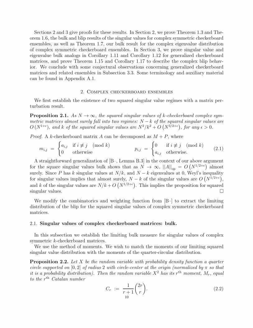
Proposition 2.2. Let X be the random variable with probability density function a quartercircle supported on [0, 2] of radius 2 with circle-center at the origin (normalized by π so thatit is a probability distribution). Then the random variable X2 has its rth moment, Mr, equalto the rth Catalan number

Cr :=1

r + 1

(

2r

r

)

. (2.2)

10

Proof. The even 2rth moments of both the semicircular distribution and the quarter-circulardistribution of X are known to equal the rth Catalan number, see for example [BS]. Theproposition then follows by noting that the rth moment of the random variable X2 is alsothe 2rth moment of random variable X .

Proof of Theorem 1.3. Before we can apply the method of moments, we must first considerthe perturbation as in the proof of Proposition 2.1, which exhibits complex symmetric k-checkerboard matrices as a finite rank (i.e., fixed as N → ∞) perturbation from the corre-sponding hollow complex symmetric k-checkerboard matrices. Then, since M + P a finiterank perturbation ofM implies that (M+P )∗(M+P ) is a finite rank perturbation ofM∗M ,we can apply Theorem 1.3 of [B–] to find that the complex symmetric k-checkerboard en-semble and the corresponding hollow ensemble have the same limiting squared singular valuedistribution. We thus apply the method of moments below to the hollow ensemble.By the eigenvalue trace lemma and linearity of expectation, the rth moment of the bulk

squared singular spectral measure is computed as

E

[

νs2(r)A,N

]

= E

[∫

νs2

A,N(x)xr dx

]

=1

NE

[

∑

σ eigenvalue B

( σ

N

)r]

= N−r−1E

[

∑

σ eigenvalue B

σr

]

= N−r−1E[

Tr(Bk)]

= N−r−1∑

1≤i1,··· ,ir≤N

E[bi1,i2 · · · bir ,i1], (2.3)

where the entries of B = A∗A are given by

bij =∑

1≤k≤N

akiakj =∑

1≤k≤N

aikakj (2.4)

by symmetry. Hence

E

[

νs2(r)A,N

]

= N−r−1∑

1≤i1≤···≤ir

E[bi1i2 · · · biri1 ]

= N−r−1∑

1≤i1,··· ,ir≤N

∑

1≤k1,...,kr≤N

E[ai1k1ak1i2 · · · airkrakri1]

= N−r−1∑

1≤i1,··· ,i2r≤N

E[ai1i2ai2i3 · · · ai2r−1i2rai2ri1 ]. (2.5)

Each term ζI = ai1i2ai2i3 · · ·ai2r−1i2rai2ri1 in the sum corresponds to a cyclic sequence I =i1 · · · i2r. Then I may be associated to a closed walk on the complete graph with verticeslabeled by the elements of the set i1, ..., i2r in the order that the vertices are visited.Define the weight of I to be the number of distinct entries of I. If the weight of I is at leastr + 2, then there is a factor a in ζI independent from all the rest, and thus the expectationE[ζI ] = 0 (recall we have zeroed out all deterministic entries because we are considering thehollow ensemble, and the random variables are all mean 0).The sequences of weight at most r contribute negligibly, o(N r+1). This is because the

sequences may be partitioned into a finite number of equivalence classes by the isomorphism11

class of the corresponding walk. An isomorphism class of weight t ≤ r then gives rise toO(N t) walks of weight t by choosing labels for the distinct nodes in any such walk.Closer analysis is required for a sequence I of weight r + 1. First, the walk corresponding

to I visits r + 1 distinct nodes and traverses r distinct edges. Hence the walk consists of 2rsteps on a tree with r + 1 nodes.Note that E[ζI ] contributes to the sum precisely when all the factors, aij , are matched

with their conjugates, aij , in which case E[ζI ] = 1. Indeed, if aij is an entry of a complexsymmetric k-checkerboard matrix A with i 6≡ j (mod k), note that E [aijaij ] = E [aijaij ] = 0while E [aijaij ] = 1. This is because if aij ∼ X + iY for X, Y iidrv mean zero variance 1/2random variables, then

E [aijaij ] = E[

X2]

+ 2iE [X ]E [Y ]− E[

Y 2]

= 0 (2.6)

E [aijaij ] = E[

X2]

+ E[

Y 2]

= 1. (2.7)

Thus it suffices to count the number of sequences I satisfying the above condition. In thegraph correspondence, the condition on I is equivalent to the walk traversing each tree edgeexactly twice, where, for an edge corresponding to i, j in I, one traversal corresponds toai,j and the other traversal to aij in ζI . For a given edge e and the corresponding subwalkw between the first and second traversal of e, each edge in w must be traversed and laterretraced in the reverse direction, since trees are acyclic. Thus w has an even number of steps,so the two traversals of e occur on steps of opposite parity.

Remark 2.3. This implies that the same result holds for the corresponding asymmetricensemble, since this parity requirement ensures that the combinatorics must be the same inboth cases.

This corresponds in ζI to matching aij with aij ; if the steps occurred with the same parity,then aij would be matched with aij (or aij with aij), resulting in zero expectation. Insummary, it suffices to count the number of non-isomorphic trees on r+1 nodes with a givenstarting node, and a given absolute order on the leaves—there is a bijection between suchwalks and such ordered trees given by the order in which the leaves are visited in the walk.As is well known, there are Cr ordered trees on r + 1 nodes, where Cr is the rth Catalan

number [S]. There is a further restriction: since aij = 0 if i ≡ j (mod k), an appearanceof any such term in the cyclic product will contribute zero expectation. We may then labelthe nodes in the tree in such a way that no two adjacent nodes have the same congruencein N r+1

(

k−1k

)r+ o(N r+1) ways. Thus we have

E

[

νs2(r)A,N

]

= N−r−1

(

∑

weight I<r+1

+∑

weight I=r+1

+∑

weight I>r+1

)

E[ζI ]

= N−r−1

(

o(N r+1) + Cr

(

N r+1

(

k − 1

k

)r

+ o(N r+1)

)

+ 0

)

= Cr

(

k − 1

k

)r

+ o(1). (2.8)

Hence we have proved

limN→∞

E

[

νs2(r)A,N

]

= Cr

(

k − 1

k

)r

= Cr

(

R

2

)2r

, (2.9)

12

which are the moments of the (square of the) quarter circle distribution of radius R =

2√

1− 1/k as in Proposition 2.2, which suffices.

2.2. Singular values of complex checkerboard matrices: blip.

Throughout this entire subsection, we follow the notation and terminology in [B–]. Forconvenience, the relevant terminology from that paper is collected in Appendix A.1. Weanalyze the blip using the method of moments.

Lemma 2.4. The expected rth moment of the EBSSSM is given by

E

[

Ms2(r)A,N

]

=1

kr+1

2n∑

j=0

(

2n

j

) r+j∑

i=0

(

r + j

i

)

(−1)r−i

(

k

N

)4n+2i+r

E[

Tr(A∗A)2n+i]

. (2.10)

Proof. By definition

E

[

Ms2(r)A,N

]

=1

kE

[

∑

σ

fn

(

k2σ

N2

)(

1

N

(

σ − N2

k2

))r]

=1

kN−r

E

[

∑

σ

fn

(

k2σ

N2

)(

σ − N2

k2

)r]

=1

kN−r

E

[

∑

σ

(

k2σ

N2

)2n(k2σ

N2− 1− 1

)2n(

σ − N2

k2

)r]

=1

kN−r

(

k2

N2

)2n

E

[

∑

σ

σ2n

2n∑

j=0

(

2n

2n− j

)

(−1)2n−j

(

k2σ

N2− 1

)j (

σ − N2

k2

)r]

=1

kN−r

(

k2

N2

)2n 2n∑

j=0

(

2n

j

) r+j∑

i=0

(

r + j

i

)(

−N2

k2

)r−i

E

[

∑

σ

σ2n+i

]

=1

kr+1

2n∑

j=0

(

2n

j

) r+j∑

i=0

(

r + j

i

)

(−1)r−i

(

k

N

)4n+2i−r

E[

Tr(A∗A)2n+i]

, (2.11)

where the last equality follows by the eigenvalue trace lemma.

Observe that the (i, j)th entry of A∗A is given by∑N

m=1 amiamj =∑N

m=1 aimamj (using thesymmetry condition of A). By definition of the trace

E [Tr(A∗A)η] =∑

1≤i1,...,iη≤N1≤m1,...mη≤N

E[

ai1k1am1i2ai2m2ak2i3 · · ·aiηmηamηi1

]

. (2.12)

Terms of the form

E [Tr(A∗A)η] =∑

1≤i1,...,iη≤N1≤m1,...mη≤N

E[

ai1m1am1i2ai2m2

am2i3 · · ·aiηmηamηi1

]

will be our cyclic products. Degrees of freedom arguments allow us to restrict our attentionto “configurations” of “1-blocks” and “2-blocks.” See Appendix A.1 for terminology taken

13

from [B–] and [B–, Lemma 3.13] for proof of the claim. We compute the contribution to theexpectation E [Tr(A∗A)η].

Lemma 2.5. The total contribution to E [Tr(A∗A)η] of an S-class C with r1 1-blocks and(|S| − r1) 2-blocks is

p(η)

(|S|r1

)

(k − 1)|S|−r1

(

1

2

)r1/2

EkTrBr1

(

(

N

k

)2η−|S|+O

((

N

k

2η−|S|−1)))

, (2.13)

where

p(η) =(2η)|S|

|S|! +O(η|S|−1) (2.14)

and the expectation E [TrBm1

k ] is taken over the k × k hollow GOE as defined in Definition1.5.

Proof. The quantity p(η) expresses the number of ways to set the position of |S| blocks(which we have established must be 1-blocks or 2-blocks) among a cyclic product of length2η which arises from E [Tr(A∗A)η]. We can estimate p(η) =

(

2η|S|)

+O(

η|S|−1)

. The term(

2η|S|)

counts the number of ways to choose positions of the blocks (ignoring overlap). The errorterm O

(

η|S|−1)

counts the number of ways in which some two blocks will be less than oneterm apart, which will occur non-generically as η → ∞.Next, the term

(|S|r1

)

counts the number of ways to choose which of the |S| blocks are

1-blocks (equivalently, the number of ways to choose which of the |S| blocks are 2-blocks).As in [B–, Proposition 3.14], the congruence classes modulo k of all the indices is completelydetermined by the choices of congruence class for the indices of the r1 1-blocks, and thefollowing (k − 1)|S|−r1 choices of congruence class for the shared index of each 2-block. Ther1 1-blocks form a cyclic product of length r1, and the number of ways of choosing thecongruence classes modulo k of their indices is equivalent to an expectation of the form

∑

1≤i1,...,ir1≤k

E[

bi1i2bi2i3 · · · bir1 i1]

= E [TrBr1k ] (2.15)

for Bk as defined prior to Theorem 1.6. This is because the number of valid choices of indexcongruence classes corresponds precisely to the number of ways to match terms in a lengthr1 cyclic product, with the restriction that consecutive indices cannot be equal (which wouldcorrespond to a deterministic entry in the original checkerboard matrix, and not a 1-blocktype entry). Further details in the argument for this reduction are similar to those in theproof of [B–, Proposition 3.14].However, our extension to singular values requires a modification to the combinatorics. As

in (2.6) and (2.7), we see that the paired entries in our cyclic product must be matched inconjugate pairs if they are to contribute to the expectation. This is automatically the casefor every 2-block, since the two terms side by side are already conjugate pairs. However, asη → ∞ and |S| remains fixed, this will be true with probability 1/2 for each pair of 1-blocks,and since there are r1/2 pairs of 1-blocks, we see that the number of valid configurations

should be scaled by(

12

)r1/2.

The last piece of the expression in Lemma 2.5 is the term(

(

Nk

)2η−|S|+O

((

Nk

2η−|S|−1)))

,

which arises from the degree of freedom count 2η−|S|−1 for the indices once we have fixed14

their congruence classes, and the big O error term arises from the lower degree of freedomterms we are ignoring, when only considering configurations of 1-blocks and 2-blocks.

Proof of Theorem 1.6. We can now compute the rth moment E[

Ms2(r)A,N

]

of the EBSSSM. By

a combinatorial lemma [B–, Lemma 3.16] copied as Lemma A.10 in Appendix A.1, we seethat only S-classes of size r contribute: if |S| > r, then the contribution vanishes in the limitof N → ∞ by a degree of freedom count, and if |S| < r, the contribution cancels via thecombinatorial lemma. Then the outer sum in Lemma 2.4 collapses to only the j = 0 term.We can substitute Lemma 2.5 into Lemma 2.4 (after adding a sum over the parameter r1which counts the number of 1-blocks in our S-class):

limN→∞

E

[

Ms2(r)A,N

]

=1

kr+1

r∑

i=0

(

r

i

)

(−1)r−ir∑

r1=0

(4n+ 2i)r

r!

(

r

r1

)

(k − 1)r−r1Ek

[

Tr

(

1√2B

)r1]

=1

kr+12r

r∑

r1=0

(

r

r1

)

(k − 1)r−r1Ek

[

Tr

(

1√2B

)r1]

. (2.16)

To compute the rth centered moments, we need the first moment:

limN→∞

E

[

Ms2(1)A,N

]

=1

k2

1∑

i=0

(−1)1−i

(

1

i

)

(4n + 2i)k(k − 1) =2(k − 1)

k. (2.17)

Thus the rth centered moments are given by

Ms2(r)c = lim

N→∞E

[∫

(

x− µs2(1)A,N

)r

dµs2

A,N

]

=

r∑

r1=0

(

r

r1

)(−2(k − 1)

k

)r−r1

limN→∞

E

[

µs2(r1)A,N

]

. (2.18)

Substituting the expression from Equation (2.16) gives

Ms2(r)c =

r∑

r1=0

(

r

r1

)

(−1)r−r1

(

2

k

)r1

k

r1∑

i=0

(

r1i

)

(k − 1)r−iEk

[

Tr

(

1√2B

)i]

.

Next, using the identity(

rr1

)(

r1i

)

=(

ri

)(

r−ir1−i

)

, we obtain

Ms2(r)c =

r∑

i=0

(

r

i

)

(k − 1)r−i

(

2

k

)r1

kEk

[

Tr

(

1√2B

)i]

r∑

r1=i

(

r − i

r1 − i

)

(−1)r−r1

=r∑

i=0

(

r

i

)

(k − 1)r−i

(

2

k

)r1

kEk

[

Tr

(

1√2B

)i]

(−1)rδmi

=

(√2

k

)r1

kEk [Tr(B)r] (2.19)

which proves Theorem 1.6 via the moment method.

2.3. Eigenvalues of complex checkerboard matrices: bulk.

15

The standard Hermitization process via the log potential is done as follows (see for ex-ample [Tao2]). Given a sequence of N × N random matrices AN with normalized spectraldistribution µ 1√

NAN

on C, we have the logarithmic potential

fN(z) :=

∫

C

log |w − z| dµ 1√NAN

(z). (2.20)

The key tool is the logarithmic potential continuity theorem.

Proposition 2.6 (Log Potential Continuity Theorem, see [Tao2]). If for almost every z ∈ C,fN(z) converges almost surely to

f(z) :=

∫

C

log |w − z| dµ(w) (2.21)

for some probability measure µ, then µ 1√NAN

converges almost surely to µ [Tao2].

Thus to show that µ 1√NAN

converges almost surely to the uniform measure µcirc on the

unit disk, it suffices to show that the log potential fN(z) converges to the correspondinglog potential of µcirc. For the checkerboard ensembles, we instead show that the re-scaledmeasure µ 1

R√NAN

converges to µcirc, where R =√

1− 1/k.

We can reduce the study of fN (z) to the spectra of Hermitian matrices by rewriting

fN(z) =1

N

N∑

j=1

log

∣

∣

∣

∣

λj(AN)√N

− z

∣

∣

∣

∣

=1

Nlog

∣

∣

∣

∣

det

(

1√NAN − zI

)∣

∣

∣

∣

=1

2

∫ ∞

0

log x dνN,z(x), (2.22)

where dνN,z(x) is the spectral measure of the Hermitian matrix(

1√NAN − zI

)∗(1√NAN − zI

)

(2.23)

for I the N ×N identity matrix. This uses the fact that

|detA| =

N∏

j=1

|λj(A)| =

N∏

j=1

λj(A∗A)1/2. (2.24)

We will analyze the spectral measure of the Hermitian matrices(

1√NAN − zI

)∗(1√NAN − zI

)

(2.25)

with the method of moments.We first have to control some convergence issues for our checkerboard ensembles, which

arise from singularities of the logarithm at 0 and ∞. The singularity at ∞ is considerablyeasier to control than the one at 0, as we will see below. Our result is conditional on thefollowing assumption on the least singular values being sufficiently far from 0, whose rolewill be made explicit in the lemma that follows.

16

Assumption 2.7. We say that a measure νN,z satisfies this assumption if

limT→∞

supN≥1

∫

|log x|≥T0<x≤1

log x dνN,z = 0. (2.26)

Remark. In the complex asymmetric case, Tao and Vu showed in 2010 that this assump-tion is satisfied via a polynomial bound on the least singular value, and a count of the othersmall singular values via the Talgrand concentration inequality, see [BC]. This difficulty ofcontrolling the singularity at 0 has traditionally been the case with the complex asymmetricensemble: Girko formulated the logarithmic potential approach in 1984 [Gi], but the circularlaw for the asymmetric ensemble remained unsolved until the behavior of the least singularvalues was sufficiently controlled by Tao and Vu in 2010 [TaoVu2]. Our complex symmet-ric checkerboard ensemble presents difficulties for the control of the small singular values -the symmetric condition (as opposed to entries being iidrv) causes the determinant to be aquadratic function of the rows (as opposed to linear in the iidrv case), and the checkerboardstructure adds further complications. See for example [CTV] for a discussion of the compli-cations introduced by imposing a symmetric structure on the matrices. Some recent workhas been done on extending the polynomial bound on the least singular value to complexsymmetric matrices [Ng] and asymmetric structured ensembles [Co], but we are not awareof any adequate generalization’s of Tao’s and Vu’s small singular value count to non iidrvmatrices. We can, however, control the singular values at ∞ for our checkerboard ensemble.

Lemma 2.8. Fix z. For matrices AN from either the complex asymmetric ensemble or thecomplex symmetric k-checkerboard ensemble, the convergence νN,z → νz implies the conver-gence of the corresponding log potentials

∫ ∞

0

log x dνN,z(x) →∫ ∞

0

log x dνz(x) (2.27)

assuming Assumption 2.7.

Proof. The condition we need is uniform integrability. For a Borel function f : E → R anda sequence ηN (x)N≥1 of probability measures on R

+, we say that f is uniformly integrablewith respect to that sequence of measures if

limT→∞

supN≥1

∫

|f |≥T

|f | dηN = 0. (2.28)

If f satisfies this condition with respect to the sequence ηN (x)N≥1 and is continuous, andthe sequence of measures converges weakly ηN → η for some probability measure η, then

limN→∞

∫

E

f dηN =

∫

E

f dη. (2.29)

For further detail see [BC].In our case, we will have (for fixed z) E = R+, ηN = νN,z, η = νz, and f(x) = log x. Since

log x has singularities at 0 and ∞, in order to satisfy uniform integrability we need to controlthe behavior of the measures νN,z at 0 and ∞. To emphasize this we split the integral:

∫

R+

log x dνN,z =

∫ 1

0

log x dνN,z +

∫ ∞

1

log x dνN,z. (2.30)

17

At infinity, we must treat the asymmetric and complex symmetric checkerboard ensemblesdifferently. For the complex asymmetric ensemble, we note that the squared singular valuesof 1√

NAN − zI are O(1) with probability 1, which trivially suffices for uniform integrability

(for sufficiently large T , νN,z has 0 mass wherever x ≥ 1 and log x ≥ T ). To control thecheckerboard ensemble at infinity, we use Weyl’s inequalities for singular values to see thatthe squared singular values of 1

R√NAN − zI have (N − k)/N mass that is O(1), and k/N

mass that is N/(R2k2) +O(

N1/2)

. This also gives uniform integrability:

limT→∞

supN≥1

∫

|log x|≥Tx≥1

|log x| dνcheckN,z ≤ limT→∞

Ck

Tlog T = 0. (2.31)

The behavior at the origin (the least singular values) is more difficult to control. However,using Assumption 2.7, which is known to be satisfied for the complex asymmetric ensemble[TaoVu2], we have uniform integrability for both the the complex asymmetric ensemble andour complex symmetric k-checkerboard ensemble.

Girko showed that, for the complex asymmetric ensemble, the corresponding νasymN,z con-verges almost surely to an explicit measure νz that satisfies

1

2

∫ ∞

0

log x dνz(x) =

∫

C

log |w − z| dµcirc(w), (2.32)

which shows the circular law, i.e., µ 1√NAN

→ µcirc almost surely, via log potential continuity

and Lemma 2.8.Thus, to show that the checkerboard ensembles have an eigenvalue bulk that converges to

µcirc, it suffices to show that our measures converge νcheckN,z → νz as well. This is accomplishedas follows.

Theorem 2.9. Let νasymN,z and νcheckN,z be probability measures with

1

2

∫ ∞

0

log x dνasymN,z (x) =

∫

C

log |w − z| dµasym1√NAN

(w)

and1

2

∫ ∞

0

log x dνcheckN,z (x) =

∫

C

log |w − z| dµcheck1

R√

NAn

(w) (2.33)

obtained as above, where µasym1√NAN

and µcheck1

R√

NAn

are the spectral measures of matrices normalized

as labeled for R =√

k−1k, and where the AN are drawn from complex asymmetric ensemble

and the complex symmetric k-checkerboard ensemble, respectively. Then as N → ∞, νasymN,z

and νcheckN,z both converge to a distribution with the same rth moments M(r)z given by

M (r)z =

r∑

j=0

c(r)j |z|2j (2.34)

for some coefficients c(r)j , where 0 ≤ c

(r)j ≤ 4rCr with Cr the rth Catalan number.

Since for almost all z, νasymN,z is known to converge as N → ∞ to a measure νz independent

of N , this allows us to conclude that νcheckN,z → νz as well.18

Proof. For any matrix AN (here AN can denote either a complex asymmetric matrix, or ahollow complex checkerboard matrix) write

BN,z :=

(

1√NAN − zI

)∗(1√NAN − zI

)

.

When studying the measures νcheckN,z , it suffices to consider instead “hollow” checkerboardmatrices AN where, for i ≡ j (mod k) we set ai,j = 0 instead of 1. This is because theoriginal checkerboard ensemble is a rank k perturbance of this modified ensemble, i.e., wecan write AN = Ahollow

N + P for a finite rank matrix P , which will also amount to a finiterank perturbance of the matrix BN,z to the analogous Bhollow

N,z . Then by [B–, Theorem 1.3]the two measures converge to the same distribution almost surely.Returning to the general setting, note that BN,z has entries

bij =

(

N∑

m=1

1√Naim − δimz

)∗(

1√Namj − δmjz

)

=1

N

N∑

m=1

amiamj −1√Naijz −

1√Najiz + δij |z|2 (2.35)

for δij the Kronecker delta (δij = 1 if i = j and is 0 otherwise).

By the eigenvalue trace lemma, the rth moment M(r)N,z of νN,z is given by the following

cyclic product :

M(r)N,z =

1

N

∑

1≤i1,...,ir≤N

E[bi1i2bi2i3 · · · biri1 ]. (2.36)

By linearity of expectation we can expand the above expectation in terms of aij using (2.35)and re-indexing. This is done via the following notation. Take Ψ : 1, 2, . . . , r → α, β, γ, δto represent an arbitrary map of sets, and write A = |Ψ−1(α)|, B = |Ψ−1(β)|, C = |Ψ−1(γ)|,and D = |Ψ−1(δ)|. Then Masym (r)

N,z and Mcheck (r)N,z can be expressed by

Masym (r)N,z =

∑

Ψ

(−1)B+CzBzC |z|2DNA+B/2+1

∑

1≤i1,...,ir≤N1≤mj≤N for j∈Ψ−1(α)

E

[

ξ(Ψ(1))1 ξ

(Ψ(2))2 · · · ξ(Ψ(r))

r

]

Mcheck (r)N,z =

∑

Ψ

(−1)B+CzBzC |z|2DR2A+BNA+B/2+1

∑

1≤i1,...,ir≤N1≤mj≤N for j∈Ψ−1(α)

E

[

ξ(Ψ(1))1 ξ

(Ψ(2))2 · · · ξ(Ψ(r))

r

]

(2.37)

where

ξ(Ψ(j))j =

amj ijamj ij+1Ψ(j) = α

aij ij+1Ψ(j) = β

aij+1ij Ψ(j) = γ

δij ij+1Ψ(j) = δ.

(2.38)

19

We also define notation to write down the conjugacy structure of the above expectation.That is, for fixed Ψ, after we factor out the Kronecker deltas δij ij+1

by collapsing the indicesij and ij+1 together, the cyclic product above will become a product of 2A+B terms of theform aij (entries of AN ) or aij (conjugates of entries of AN .) Each aij or aij will be referredto as a term. Then, for 1 ≤ j′ ≤ 2A+B (j′ indices meant to enumerate mj indices as well),let ψ+ denote those indices j′ such that the j′th term in the product is an entry from AN ,and let ψ− denote those indices j′ such that the j′th term in the product is an entry fromAN .

Example 2.10. The function 1, 2, 3, 4, 5, 6, 7 Ψ−→ β, β, α, δ, γ, γ, α corresponds to thecyclic product E [(ai1i2) (ai2i3) (am3i3am3i4) (δi4i5) (ai6i5) (ai7i6) (am7i7am7i1)].

We can now give a different characterization of the above expectations. Below, we use thephrase step to refer to each traversal of an edge in a walk on a graph. First we specialize tothe complex asymmetric case.

Lemma 2.11. For AN from the complex asymmetric ensemble and for fixed Ψ, as N → ∞the expectation

1

NA+B/2+1

∑

1≤i1,...,ir≤N1≤mj≤N for j∈Ψ−1(α)

E

[

ξ(Ψ(1))1 ξ

(Ψ(2))2 · · · ξ(Ψ(r))

r

]

. (2.39)

counts the number of non-isomorphic closed walks on trees with A+B/2+1 nodes such that

• if B/2 is not an integer then this quantity is understood to be zero,• each edge is traversed exactly twice (once in each direction),• each step is given a sign ±, and• if some edge is traversed first on the j′1

th step and then later on the j′2th step, then

either j′1 has positive sign and j′2 has negative sign, or vice versa.

We refer to such walks as signed closed walks on trees.

Proof. First, note that in such a cyclic product there will be 2A+B terms and 2A+B indices,once we have collapsed the indices corresponding to Kronecker delta terms δij . Suppose weset some of the indices to be equal, so that there are ℓ free indices for 1 ≤ ℓ ≤ 2A + B.If ℓ < A + B/2 + 1, then the contribution vanishes in the limit N → ∞. Else, define agraph on ℓ vertices by drawing an edge between vertices i and j if there exists a term withindices i and j (respecting the given identification of vertices/indices). There must be atleast ℓ− 1 edges, and if ℓ > A+B/2 + 1, then there are more than A+B/2 distinct edges.By construction, two distinct edges are given by two independent terms. Thus, there aremore than A + B/2 terms in our cyclic product, so that there exists one term independentfrom the rest. Note that all terms are drawn from mean 0 distributions, so that if any oneterm is independent from the rest, then the entire expectation is immediately zero. So weconclude that, for a nonzero expectation, our graph will contain A + B/2 + 1 vertices andA + B/2 edges, and thus is a tree on A + B/2 + 1 nodes. We show first that every cyclicproduct of nonzero expectation corresponds to a walk satisfying the above conditions.Define a walk on this tree as follows (see Figure 3 for a useful example). Start at the

index corresponding to i := i1. If the first term is aij , walk from vertex i to vertex j, andassign this step a + sign. If instead the first term is aji, also walk from vertex i to vertex j,but assign this step a − sign. These are the only possibilities. By construction, the cyclic

20

i1=i7

m7

i2=m3=i6

i3 i4=i5

1

23 4

5

67

8

Figure 3. The graph associated to the cyclic product from Example 2.10if we consider the matching i1 = i7, i2 = m3 = i6, and i4 = i5 (which isvalid, i.e., gives nonzero expectation). The arrows represent steps of the walk,numbered in order, with dotted arrows representing steps of negative sign andsolid arrows representing steps of positive sign.

product above will yield a walk on the constructed tree with A+B/2 edges. Since we startedwith 2A+B edges, each edge is traversed exactly twice. For the third condition, note by thecomputations in (2.6) and (2.7) that two dependent terms (i.e., the two times we traversethe same edge) with a nonzero expected product must be of different conjugacy classes (i.e.,one is an entry from AN , and another is an entry from AN ). This translates to the thirdcondition above: since the sign of each step keeps track of the conjugacy class that gave thatstep, this means that the two steps for every edge must have opposite sign.Now we claim that every walk on a tree with A+B/2 nodes satisfying the above conditions

corresponds to a cyclic product with nonzero expectation. Given such a walk, with first stepfrom i to j, set the first term in the cyclic product to be aij if the step has sign +, and aji ifthe step has sign −. Doing this for all steps will generate a cyclic product where every termis paired with exactly one other term, in a conjugate pair. To ensure we count only terms ofnonzero expectation, we need to check that all conjugate pairs are of the form E[aijaij ] = 1and not E[aijaji] = 0, since we are working with a complex asymmetric ensemble, and aij isindependent from aji. However, the second situation cannot happen, since our walk occurson a tree, i.e., if each edge is traversed exactly twice, the two steps must occur in oppositedirections, so one step goes from i to j, while the other goes from j to i. Then, forcing thesteps to have opposite signs implies our paired expectations are of the form E[aijaij] = 1.This shows the bijection between our cyclic expectations and walks satisfying the aboveconditions.Then, once we have fixed a valid identification of the starting 2A+B indices to A+B/2+1

free indices, each free index hasN choices (un-identified indices being assigned the same indexwill happen non-generically as N → ∞ for r fixed, and will vanish in the limit as lower orderterms by degree of freedom counts as above), so each nonzero expectation will contributeNA+B/2+1 which equals 1 after dividing out by the normalizing factors of N present above,which suffices for the lemma.

21

Corollary 2.12. For AN from the complex symmetric k-checkerboard ensemble and for fixedΨ, Lemma 2.11 holds for the analogous expectation:

1

R2A+BNA+B/2+1

∑

1≤i1,...,ir≤N1≤mj≤N for j∈Ψ−1(α)

E

[

ξ(Ψ(1))1 ξ

(Ψ(2))2 · · · ξ(Ψ(r))

r

]

. (2.40)

Proof. The interpretation of cyclic products as walks as above for aij entries of checkerboardmatrices is similarly valid up to the last two paragraphs of the proof of Lemma 2.11.It is clear that every identification of indices that gives a nonzero expectation for the

asymmetric ensemble also gives a nonzero expectation for the symmetric ensemble. Weshould check that we can find no additional matchings from the symmetric condition. Thisis something we have already seen: above, we argued given a walk satisfying the aboveconditions and the associated cyclic product it generates, none of the pairings in the cyclicproduct are of the form E[aijaji], because of the restriction that steps on the same edge areof opposite sign.However, we have an additional restriction that when choosing our indices, if there exists

an edge between i and j, then i 6≡ j (mod k). This is because if i ≡ j (mod k) thenaij = 0, and the expectation is zero. The modification is clear from the interpretation ofwalks on a tree: since trees are acyclic, once we have fixed the congruence class of onevertex, (recalling ℓ = A + B/2 + 1 there will be (k − 1)ℓ−1 ways to choose congruenceclasses of the other vertices such that adjacent vertices on the tree do not share the samecongruence class, so there are k(k − 1)ℓ−1 ways to choose the congruence classes. Afterfixing the congruence classes there are (N/k)ℓ ways to choose indices for each vertex, so we

see there are N ℓ(

k−1k

)ℓ−1= NA+B/2+1R2A+B ways to choose the vertices that will give a

nonzero expectation. Dividing by the normalizing factors of N and R in front then give theresult.

This shows that for all z ∈ C, limN→∞Masym (r)N,z = limN→∞M

check (r)N,z . A few observations

reduce the moments to the form claimed in Theorem 2.9. Since above we saw that every termmust be paired with exactly one other conjugate term to produce a nonzero expectation, weconclude B = C, so our moments must take the form claimed in Theorem 2.9.

Remark 2.13. Note that the proof of Corollary 2.12 also goes through for the complex asym-metric k-checkerboard ensemble. Because of the restriction of matching terms in conjugatepairs, the symmetry condition is immaterial for this specific bulk calculation as is discussedabove.

Corollary 2.14. We have 0 ≤ c(r)j ≤ 4rCr with Cr the rth Catalan number.

Proof. Note that there are 4r choices of Ψ. Then, since A+B/2+1 ≤ r+1 and the numberof non-isomorphic closed walks on trees with r + 1 nodes such that each edge is traversedexactly twice is given by Cr (equivalently the number of ordered trees on r + 1 nodes), weobtain the claimed upper bound via Lemma 2.11 and Equation (2.37). Note that this upperbound is far from tight, as we have not removed any walks corresponding to zero expectation,from the assignment of signs to steps.

Example 2.15. The coefficients c(r)j can be computed by hand. For example, there is one

choice of Ψ such that B + C + 2D = 0 (i.e., A = r), which corresponds to signed closed22

walks on trees with r nodes. Then, as in the proof of Theorem 1.3, every closed walk on atree where every even step has sign + and every odd step has sign − always satisfies thecondition that the two steps on the same edge are of opposite sign, i.e., the number of valid

walks is counted by the Catalan number Cr, so we conclude c(r)0 = Cr. There is also only

one choice of Ψ such that B+C+2D = 2r (i.e., D = r), which corresponds to signed closed

walks on trees with one node, of which there is one, so c(r)r = 1.

Example 2.16. The first few moments are

M (1)z = 1 + |z|2

M (2)z = 2 + 3 |z|2 + |z|4

M (3)z = 5 + 15 |z|2 + 6 |z|4 + |z|6 . (2.41)

In particular, Corollary 2.14 implies that Carleman’s condition is satisfied for our momentsat each fixed z, since for fixed z the moments are bounded by some scaling of the Catalannumbers (which satisfy Carleman’s condition as in Wigner’s semicircle law). Thus the mo-ments uniquely characterize the distribution for every fixed z, i.e., νcheckN,z → νz and we haveproved Theorem 2.9.

Proof of Theorem 1.7. Applying Proposition 2.6 and Lemma 2.8 to Theorem 2.9 suffices forthe proof of Theorem 1.7.

3. Generalized checkerboard ensembles

3.1. Analogs of bulk and blip results for generalized checkerboard ensembles.

The ensembles that follow in this subsection will have random variables iidrv (up to asymmetry restriction). Many of the main results above hold for generalized checkerboardensembles as well.

Proof of Corollary 1.11. As in the proof of Theorem 1.3 we can reduce to the case wherethe deterministic entries are all zero by a perturbation argument, apply the eigenvalue tracelemma up to Equation (2.5), and also interpret the cyclic products as closed walks on treeswith r+1 nodes. The number of closed walks traversing each edge twice on trees with r+1nodes is again given by the number of ordered trees on r + 1 nodes, which is Cr. As before,it is not true that all N r+1+O (N r) choices of indices will yield a nonzero expectation in thecyclic product, since if i and j are adjacent indices then we cannot have aij = 0. Before, thisreduced to the condition i 6≡ j (mod k). In the m-regular k-checkerboard case, however,the correct condition is that, having fixed any congruence class modulo k of some index i,there are k −m congruence classes for the index j such that aij 6= 0. This is because m isa constant dependent only on the entire ensemble. Thus we see that (R/2)2rN r+1 +O (N r)choices of indices will yield a nonzero expectation in the cyclic product. Indeed, there are Nchoices for the root of the tree, N(1 −m/k) choices for each of their children, N(1 −m/k)choices for each of the children in the next level down, etc., which shows that all moments

of the squared singular value bulk are Mr =(

R2

)2rCr as claimed.

Example 3.1. In general, a non-regular generalized k-checkerboard ensemble need not havesingular values following a quarter-circular bulk. Consider the generalized 2-checkerboard

23

ensemble tiled with 2× 2 matrices of the form(

1 ∗∗ ∗

)

(3.1)

where, as before, each ∗ represents an iidrv complex random variable with mean 0 variance1/2 that respects the symmetric structure . As in the proof of Theorem 1.3 the bulk of thisensemble will converge to the bulk of the ensemble with the entries 1 replaced with 0. Bruteforce computing the small moments (counting by hand the appropriate walks on trees as isdone to compute the quarter-circular bulk above) gives M1 = 3/4, M2 = 10/8, M3 = 42/16,and M4 = 198/32. In particular the bulk cannot be quarter-circular of radius R, whichwould correspond to moments Mr = (R/2)2rCr, e.g. M1 = (1/2)(R2/2), M2 = (2/4)(R4/4),M3 = 5/8(R6/8), and M4 = (14/16)(R8/16).2

Proof of Corollary 1.12. The discussion of the log potential in the proof of Theorem 1.7 isdone in the same way for our generalized checkerboard ensemble up to Lemma 2.8. The proofof that lemma goes through as well, assuming the appropriate analogy to Assumption 2.7(replace instances of the checkerboard ensemble with the generalized checkerboard ensemble),when we note that Weyl’s inequality for singular values of 1√

NAN − zI for fixed z gives at

least N−k squared singular values of size O (1), and at most k squared singular values of sizeO (N), in which case the argument in Lemma 2.8 for the behavior at ∞ can be applied aswell. The qualifiers “at least” and “at most” come from the fact that the perturbation fromthe hollow ensemble (deterministic 1’s replaced with 0’s) for a generalized k-checkerboard isrank at most k, possibly less.Then, the expansions of Theorem 2.9 in the checkerboard context can also be done for the

generalized checkerboard ensembles, with the necessary modifications arising in an analogousproof of Corollary 2.12. As discussed in that proof, the restriction of symmetry on theensemble does not affect the combinatorics that arise when counting signed closed walks ontrees. Again, the modification comes when counting how many ways there are to chooseindices, given a walk, since adjacent indices i, j must have aij 6= 0 for the expectation to benonzero as discussed in the proof of Corollary 2.12. Here, there are N ways to choose theindex of the root, R2N ways to choose the indices of the root’s children, RN ways to choosethe indices of those children’s children, etc. which shows as in Corollary 2.12 that the bulkconverges to a uniform disc centered at the origin scaled by R.

3.2. Eigenvalues of complex checkerboard matrices: blip.

The main steps in the proof of Theorem 1.15 are to first restrict our attention to regionsΩǫ to avoid the singularity at 0, show that the distribution must be discrete and finitelysupported, show that discrete distributions are characterized by (holomorphic) moments,compute moments via the eigenvalue trace lemma, and to control the error arising fromrestricting to Ωǫ.

Lemma 3.2. For all ǫ > 0, assume almost sure convergence to some measure µN → µ asmeasures on Ωǫ. With any fixed ǫ > 0, the measure µ on Ωǫ must be a discrete measure withfinite support.

2We note that the numerators (starting with the 0 − th moment) 2, 3, 10, 42, 198 are the first five terms ofthe OEIS sequence A007226, which relates to counting certain ternary trees.

24

Proof. Consider 0 < ǫ′ < ǫ and write µN and µ′N for the restrictions to Ωǫ and Ωǫ′ respectively.

Write also µN → µ and µ′N → µ′ via our convergence assumption. Note µ′ restricts to µ on

Ωǫ.Write p(x) for the (degree k) characteristic polynomial of B, and define f(z) := zp(z),

viewed as a function f : C → C. Note f has fixed degree as N → ∞.Consider the pushforward measures f∗µ

′N → f∗µ

′ on f(Ωǫ′). Note that f∗µN is also thespectral distribution of f

(

kNAN

)

restricted to f(Ωǫ′) with total (restricted) measure scaledby N/k, and in particular has the same support. We can control the support of the spectraldistribution of f

(

kNAN

)

via its largest singular value, which majorizes all its eigenvalues.

If c is the constant term of p(z), the Cayley-Hamilton theorem shows that p(

kNP)

− c is ablock matrix consisting of repeating k×k identity blocks scaled by −kc/N . This then showsf(

kNP)

= 0. Note f(

kNAN

)

= f(

kNP)

+ O(

kNM)

= O(

kNM)

, where the big O term is a

sum of mixed products of kNM and k

NP at least linear in k

NM . The number of terms in this

sum is fixed as N → ∞ because f has fixed degree. The largest singular value of kNP is

O(1) and the largest singular value of kNM is almost surely O(N−1/2+ǫ) for all ǫ > 0 via a

standard method of moments argument, see the proof of Proposition 2.1 and Lemma B.3 of[B–] (recall that M has all deterministic entries set to zero).3

Thus the largest singular value of f(

kNAN

)

is almost surely O(

N−1/2+ǫ)

for all ǫ > 0.

In particular, as N → ∞ the spectral measure of f(

kNAN

)

and thus f∗µ′N almost surely

has support contained in any fixed radius ball at the origin. Considering the neighborhoodf(Bǫ′) of the origin, we find that f∗µ

′N is almost surely supported on f(Bǫ′) as N → ∞.

Fixing any δ > 0, we can then select ǫ′ > 0 small such that f∗µ′N vanishing outside f(Bǫ′)

implies that, on Ωǫ′ , µ′N vanishes outside balls of radius δ centered at the zeroes of f .4

Since µ′N restricts to µN on Ωǫ as long as ǫ′ < ǫ, sending δ → 0 and then N → ∞ shows

that µ, restricted to Ωǫ is finitely supported at the (nonzero) zeroes of f .

We would like to analyze the moments of µN → µ. However, the formula from theeigenvalue trace lemma applies to moments of µN on all of C rather than restricted Ωǫ. Wefirst control this error.

Lemma 3.3. As N → ∞, the measure µN restricted to Bǫ contributes at most (1/k)(2k+2)ǫto the rth moments, for r ≥ 6.

Proof. Applying Weyl’s inequalities as in Proposition 2.1 shows that, almost surely, thek largest singular values of AN are O(N) and the remaining N − k singular values areO(N1/2+ǫ). Recall that the product of the m largest singular values majorizes the product ofm largest eigenvalues. The m product of the m largest eigenvalues of AN thus have growtho(

Nk+(m−k)3/5)

as N → ∞. Thus the total measure of µN outside of BN−1/5 is boundedabove by (1/k)(2k+ 1) as N → ∞ since m(4/5) > k+ (m− k)(3/5) when m ≥ 2k+1. Themeasure µN restricted to the region outside of BN−1/5 but within Bǫ thus contributes at most(2k + 1)ǫ to any positive moments, while the measure µN restricted to BN−1/5 contributesat most N · N−6/5 = O(N−1/5) to rth moments for r ≥ 6 as N → ∞, which we bound by(1/k)ǫ. Adding these two contribution gives the claimed bound.

3This bound alternately follows from the Gershgorin Circle Theorem applied to M – central limit theoremon the at most N random variables in each row gives Gershgorin discs of radii O(N1/2) with centers atdistance O(1) from the origin.4Note C \ f(Ωǫ′) ⊂ f(Bǫ′) by surjectivity of f .

25

Remark 3.4. The part of the proof of Lemma 3.3 bounding the total measure outside BN−1/5

also shows that µ viewed as a measure on Ωǫ has finite total measure, for all ǫ > 0.

We next show how the (holomorphic) moments characterize discrete distributions.

Lemma 3.5. Any finite discrete measure µ on C with finite support in C \ 0 is uniquelydetermined by its rth integer moments for r ≥ α, for any fixed integer α > 0.

Proof. Given distinct nonzero complex numbers zjnj=1 with nonzero coefficients λjnj=1,and distinct nonzero complex numbers and z′kmk=1 with nonzero coefficients λ′kmk=1 suchthat

n∑

j=1

λjzrj =

m∑

k=1

λ′kz′rk (3.2)

for all r ≥ N , we wish to show that n = m and, for some appropriate permutation of theindices, λj = λ′k for j = k, and zj = z′k for j = k.We can associate to any complex number z the sequence z = (zα, zα+1, zα+2, . . .) ∈ CN.

Then Equation (3.2) becomesn∑

j=1

λjzj =

m∑

k=1

λ′kz′k. (3.3)

Under the left-shift linear operator in the sequence space CN, note that z is a nonzero eigen-vector with eigenvalue z. In particular, sequences associated with distinct complex numbershave distinct eigenvalues and are thus linearly independent. Applying this to Equation (3.3)gives the claim.

Lemma 3.6. The expected rth moments E[

M(r)N

]

converge to the rth moment of the spectral

measure of the deterministic k × k matrix B as N → ∞.

Proof. Write M(r)N for the rth moment of µN . By the eigenvalue trace lemma, the expected

rth moment is given by

E

[

M(r)N

]

=N

k

1

N

kr

N r

∑

1≤i1,...,ir≤N

E [ai1i2 · · · airi1] . (3.4)

We analyze this with a standard degree of freedom count. Fix a cyclic product E [ai1i2 · · · airi1 ].Consider some aij appearing in this cyclic product that corresponds to a random variable,i.e. not a deterministic entry of the matrix. If aij is independent from the the other entries,the contributed expectation is zero since the random variables in the matrix ensemble havemean 0. Else, aij matches another term in the cyclic product, which loses at least one degree

of freedom for the indices. In particular, such a contribution to E

[

M(r)N

]

must be O(1/N)

which vanishes as N → ∞.Thus, as N → ∞, the quantity E

[

M(r)N

]

can be computed only considering cyclic products

with all entries deterministic. Reducing modulo k (and recalling that the deterministic entriesof k-checkerboard matrices repeat modulo k)

E

[

M(r)N

]

=1

k

∑

1≤i1,...,ir≤k

E [ai1i2 · · · airi1] (3.5)

26

where the expectations E [ai1i2 · · · airi1 ] are understood to be taken over deterministic entriesonly. This is precisely the rth moment of the spectral measure of the matrix B as claimed.

Proof of Theorem 1.15. Fix ǫ > 0 and consider 0 < ǫ′ < ǫ. By Lemma 3.3 the rth moments ofµ on Ωǫ′ differ from the rth moments of the spectral measure of B by at most (1/k)(2k+2)ǫ′,when r ≥ 6. Since µ on Ωǫ restricts to µ on Ωǫ′ when ǫ

′ < ǫ, and µ is supported on the zeroesof f , the rth moments of µ on Ωǫ are equal to the rth moments of µ on Ωǫ′ whenever ǫ issmaller than the smallest nonzero eigenvalue of B (i.e. smallest nonzero zero of f). Sendingǫ′ → 0 shows that the rth moments of µ on Ωǫ must be equal to the rth moments of thespectral measure of B restricted to Ωǫ when r ≥ 6. By Lemma 3.2, µ on Ωǫ is a discretemeasure with finite support at the nonzero zeroes of f . By Remark 3.4 the total measure isfinite. Lemma 3.5 shows that these two measures must be equal as claimed.

Proof of Corollary 1.17. By Theorem 1.15, the k′ largest eigenvalues of AN are all of sizeO(N). Applying Weyl’s inequalities as in Proposition 2.1 shows that, almost surely, thek′ largest singular values of AN are O(N) and the remaining N − k′ singular values areO(N1/2+δ). The product of the m largest singular values majorize the product of the mlargest eigenvalues, which suffices for the claim with a similar argument as in the proof ofLemma 3.3.

3.3. Conjectures.

Although in Section 3 we only analyzed ensembles resulting in “discrete-type” blip dis-tributions, it is natural to ask whether we can naturally construct other ensembles wherethe resulting blip distribution will not be discrete. For example, if we modify the complexk-checkerboard ensemble and replace the deterministic 1’s with complex numbers on the unitcircle, drawn with uniform probability, our result trivially implies that the blip will consistof a ring of eigenvalues on the unit circle, in the same sense of Theorem 1.15; see Figure 1(right).One can attempt to construct non-discrete blip distributions in other ways, for example

with an analogy of a generalized complex k-checkerboard ensemble with B matrix havingeigenvalues at the k-th roots of unity, except where k =

√N is growing as N → ∞ over the

squares. Heuristically, one expects the blip distribution to be a ring of vanishing thickness,in some sense, but one would need different techniques than those used to describe thediscrete-type blip distributions characterized by Theorem 1.15.As a final note, the bulk also seems to deviate from standard circular law behavior in more

general ensembles when, for example the entries are no longer iidrv, and different entries areassigned different means or variances. Instead we observe some sharpened bulk distributions,that are distinctly non-uniform.

Appendix A.

A.1. Notation and terminology for cyclic products. Throughout we have used someconvenient terminology borrowed from [B–] to analyze the cyclic products. The definitionsare copied and adapted below.Recall that

E [TrMn] =∑

1≤i1,...,in≤N

E[mi1i2mi2i3 · · ·mini1 ]. (A.1)

27

Figure 4. Sharp bulkdistribution, two differentvariance values for therandom entries.

Figure 5. Three differentvariance values for the ran-dom entries. There appearto be three bulks “stacked”on top of each other.

We refer to terms E[mi1i2mi2i3 · · ·mini1] as cyclic products and m’s as entries of cyclicproducts. Occasionally, some of our cyclic products appear in altered form, with certainterms mij ij+1

replaced instead with mij+1ij or perhaps with complex conjugates mijij+1or

mij+1ij , but we extend this terminology to those scenarios as well. In many of our momentarguments, we are interested in computing these cyclic products, which reduces to a combi-natorics problem of understanding the contributions of different cyclic products. We developthe following vocabulary to classify types of cyclic products according to the aspects of theirstructure that determine overall contributions.

Definition A.1. A term refers to a single component mijij+1of the cyclic product.

Definition A.2. A block is a set of adjacent a’s surrounded by w’s in a cyclic product,where the last entry of a cyclic product is considered to be adjacent to the first. We refer toa block of length ℓ as an ℓ-block or sometimes a block of size ℓ.

Definition A.3. A configuration is the set of all cyclic products for which it is specified(a) how many blocks there are, and of what lengths, and (b) in what order these blocksappear. However, it is not specified how many w’s there are between each block.

Example A.4. The set of all cyclic products of the form w · · ·waw · · ·waaw · · ·waw · · ·w,where each · · · represents a string of w’s and the indices are not yet specified, is a configu-ration.

Definition A.5. Let S be a multiset of natural numbers. An S-class, or class when S isclear from context, is the set of all configurations for which there exists a unique s-block forevery s ∈ S counting multiplicity. In other words, two configurations in the same class musthave the same blocks but they may be ordered differently and have different numbers of w’sbetween them.

Definition A.6. Given a configuration, a matching is an equivalence relation ∼ on the a’sin the cyclic product which constrains the ways of indexing (see Definition A.9) the a’s asfollows: an indexing of a’s conforms to a matching ∼ if, for any two a’s aiℓ,iℓ+1

and ait,it+1,

we have iℓ, iℓ+1 = it, it+1 if and only if aiℓiℓ+1∼ ait,it+1

. We further constrain that eacha is matched with at least one other by any matching ∼.

28

Remark A.7. Noting that the aij are drawn from a mean-0 distribution, any matching withan unmatched a would not contribute in expectation, hence it suffices to only consider thosewith the a’s matched at least in pairs.

Example A.8. Given a configuration ai1i2wi2i3ai3i4wi4i5ai5i6wi6i7ai7i8wi8i1 (the indices arenot yet specified because this is a configuration), if ai1i2 ∼ ai5i6 we must have either i1 = i5and i2 = i6 or i1 = i6 and i2 = i5.

Definition A.9. Given a configuration, matching, and length of the cyclic product, thenan indexing is a choice of

(1) the (positive) number of w’s between each pair of adjacent blocks (in the cyclic sense),and

(2) the integer indices of each a and w in the cyclic product.

Lemma A.10. (Lemma 3.16 from [B–].) For any 0 ≤ p < mm∑

j=0

(−1)j(

m

j

)

jp = 0. (A.2)

Furthermorem∑

j=0

(−1)m−j

(

m

j

)

jm = m!. (A.3)

A.2. Joint density for singular values of complex symmetric Gaussian ensemble.We give a proof of the joint density of singular values for complex symmetric matrices foundin [AZ, Fo].

Theorem A.11 (Joint Density of Singular Values for Complex Symmetric Matrices). Sup-pose M is a random complex symmetric N × N matrix (not necessarily Hermitian), withentries in the upper triangle half and the diagonal iidrv mean 0 variance 1 complex Gaussianrandom variables. The joint density of the singular values of M is given by

ρN(x1, . . . , xN) = cN∣

∣∆(x21, . . . , x2N )∣

∣

N∏

j=1

|xj |N∏

j=1

e−|xj |2/2. (A.4)

We adapt a proof of Ginibre’s formula for the eigenvalue joint density of complex asym-metric matrices as presented by Stephen Ge [Ge], who cites Mehta [Me, DM].

Proof of Theorem A.11. Let |M |2 = Tr(M∗M) denote the Frobenius (Hilbert-Schmidt)norm. Then

dP := CNe−|M |2/2 dM = CN

∏

i,j

e−|xij |2/2 dM (A.5)

gives M ’s density on the space of all n × n complex symmetric matrices, where dM isLebesgue measure on that space and Cn is some constant.We derive the desired formula by computing P(|M − D′| ≤ ǫ) in two ways, for ε > 0

arbitrarily small and D′ a fixed diagonal matrix with non-negative real entries. The abovedensity gives

P(|M −D′| ≤ ǫ) =

∫

|M−D′|≤ǫ

dP. (A.6)

29

We can treat this integral as the volume of a thin rectangle centered at D’, since ǫ is verysmall. Since we takeM from a distribution of complex symmetric matrices, and such matriceshave N2 +N degrees of freedom, this volume is bounded above by Cne

−|D′|2/2ǫN2+N . Thus

we have

P(|M −D′| ≤ ǫ) = (C + o(1))e−|D′|2/2ǫN2+N . (A.7)

We now compute this probability a second way by using the Takagi factorization of acomplex symmetric matrix M :

M = UDU⊺, (A.8)

where U is unitary and D is a diagonal matrix with nonnegative real entries. Since unitarymatrices U can be written as U = exp(S) for some S skew Hermitian, U has N2 degreesof freedom, while D has N . Thus, the left and the right-hand sides of (A.8) have the samenumber of degrees of freedom.Define a density ψ(D)dD on the space of diagonal matrices with nonnegative real entries,

so that when U is taken from the unitary group uniformly and D with density ψ(D), M =UDU⊺ is a Gaussian random matrix. We eventually use both probability expressions tocompute ψ(D), which will in turn allow us to determine the joint density formula.Now, let M be such that |M − D′| ≤ ǫ. Then, following the lead of Tao [Tao1], we

write U = I + O(ǫ) and D = D′ + εE, where E is real diagonal. After counting degrees of

freedom, S has density C ′(1 + o(1))ǫN2

dS, where dS is the Lebesgue measure on the spaceof skew-Hermitian matrices. Similarly, E has density C ′′(1 + o(1))ǫnψ(D′)dE. We have

M = UDU⊺

= exp(ǫS)(D′ + ǫE)exp(ǫS)⊺

= exp(ǫS)(D′ + ǫE)exp(ǫS⊺)

= exp(ǫS)(D′ + ǫE)exp(−ǫS). (A.9)

Thus we can write

P(|M −D′| ≤ ǫ) = C ′′′∫ ∫

|exp(ǫS)(D′+ǫE)exp(−ǫS)−D′|≤ǫ

(1 + o(1))ǫN2

dSǫNψ(D′) dE

= C ′′′ǫN2+N(1 + o(1))ψ(D′)

∫ ∫

|exp(ǫS)(D′+ǫE)exp(−ǫS)−D′|≤ǫ

dSdE.

(A.10)

Taylor-expanding the exponential to first order gives

|exp(ǫS)(D′ + ǫE)exp(−ǫS)−D′| = |(D′ + ǫSD′ + ǫE − ǫD′S +O(ǫ2))−D′|= |ǫ(E + SD′ −D′S +O(ǫ))|. (A.11)

which from above we want to be at most ǫ. As |B|2 = Tr(B∗B), this implies that

|E + SD′ −D′S| ≤ 1 +O(ǫ). (A.12)

Consider the change of variables

A = E + SD′ −D′S. (A.13)

30

Entry-by-entry, we have

Ajk = Ejk + (D′kkSjk −D′

jjSjk). (A.14)

Here we have used the fact that D′ is diagonal. Also, the skew-symmetry of S and thediagonality of E and D′ imply Ajk is symmetric.Next, we write the real and imaginary parts of this change of coordinates separately. Let

σAjkdenote the real part of Ajk, and τAjk

denote the imaginary part of Ajk. Recalling thatD is real diagonal, we have

σAjk= σEjk

+ σSjk(σD′

kk− σD′

jj)

τAjk= τSjk

(σD′kk+ σD′

jj). (A.15)

We can interpret this matrix change of variables A → (S,E) as a transformation from

Rn2+n to R

n2+n, i.e., from (for j ≤ k) the σAjkand τAjk

to n2 + n-tuples with entries σSjk

(for j < k), τSjk(for j ≤ k), and σEjj

. This transformation is a direct sum of three diagonaltransformations:

σAjk= σSjk

(σD′kk− σD′

jj) for j 6= k

σAjj= σEjj

τAjk= τSjk

(σD′kk+ σ′

D′jj). (A.16)

This is a diagonal transformation, i.e., its Jacobian is the product of each of the above scalingfactors. The Jacobian for the change of coordinates (S,E) → A is

∏

1≤j<k≤n

|D′2kk −D′2

jj|n∏

j=1

|2D′jj| = |∆(D′2

11, . . . , D′2nn)|−1

n∏

j=1

|2D′jj|−1. (A.17)

Returning to (A.10), we have

P(|M −D′| ≤ ǫ) = C ′′′ǫN2+N(1 + o(1))ψ(D′)

∫ ∫

|exp(ǫS)(D′+ǫE)exp(−ǫS)−D′|≤ǫ

dSdE

= C ′′′ǫN2+N(1 + o(1))ψ(D′)

∫

|A|≤1+O(ǫ)

dA. (A.18)

Note that as ǫ→ 0, the integral in A goes to a constant. Absorbing this into the constantC ′′′ and comparing the above expression for P(|M −D′| ≤ ǫ) with (A.7) gives

ψ(D′) = C ′′′′|∆(D211, . . . , D

2nn)|

(

N∏

j=1

|2D′jj|)

e−|D′|2/2

= C ′′′′|∆(D211, . . . , D

2nn)|

N∏

j=1

|2D′jj|

N∏

j=1

e−D′2jj/2. (A.19)

As the diagonal entries Djj are precisely the singular values of M , we find

ρn(x1, . . . , xN) = C ′′′′ ∣∣∆(x21, . . . , x

2N)∣

∣

N∏

j=1

|2xj |N∏

j=1

e−|xj |2/2, (A.20)

which proves the theorem after absorbing 2N into the constant.

31

Theorem A.11 allows us to compute the distribution of the least singular value for theGaussian complex symmetric ensemble. As before, we list the available distribution for theleast singular values of the complex asymmetric Gaussian ensemble as computed by Edelman[Ed]:

Complex asymmetric Gaussian : p(σN) = NσNe−Nσ2

N/2 (A.21)

Corollary A.12. The probability density function of the least singular value σN follows theRayleigh distribution

p(σN) = NσNe−Nσ2

N /2. (A.22)

Note that, while the joint densities are distinct, the least singular value of the complexasymmetric and complex symmetric Gaussian matrices share the same distribution.

Proof of Corollary A.12. Order the singular values 0 ≤ σN ≤ · · · ≤ σ1. Using Theorem A.11,we can integrate out the other parameters σ1, . . . , σN−1 from the joint density to obtain thedensity function of the least singular value:

p(σN ) =

∫

σN≤σN−1≤···≤σ1

ρN(σ1, σ2, . . . , σN) dσ1 · · ·dσN−1

= CN

∫

σN≤σN−1≤···≤σ1

∏

1≤k<j≤N

(

σ2k − σ2

j

)

N∏

j=1

σj

N∏

j=1

e−σ2j /2 dσ1 · · · dσN−1

= CNσNe−Nσ2

N/2

∫

σN≤σN−1≤···≤σ1

∏

1≤k<j≤N−1

(

σ2k − σ2

j

)

∏

1≤k≤N−1

(

σ2k − σ2

N

)

·n∏

j=2

σj

n∏

j=2

e−(σ2j−σ2

N )/2 dσ1 · · · dσN−1. (A.23)

As is done in [Ed], make the change of variables xj = σ2j − σ2

N . Thus, with dxj = 2dσj, wefind

p(σN ) = 21−NCNσNe−Nσ2

N/2

∫

0≤xN−1≤···≤x1

∏

1≤k<j≤N−1

(xk − xj)N−1∏

j=1

xj

N−1∏

j=1

e−xj/2 dx1 · · ·dxN−1.

(A.24)

Since the integral is independent of σN , it is constant, which we denote by C ′N :

p(σN) = C ′NσNe

−Nσ2N/2. (A.25)

As p is a probability distribution,∫

R≥0p(σN ) dσN = 1 and thus C ′

N = N , completing the

proof.

References

[AZ] A. Altland and M. Zirnbauer, Novel Symmetry Classes in Mesoscopic Normal-SuperconductingHybrid Structures, Phys. Rev. B 55 (1997), 1142–1161.

[Bai] Z. Bai, Methodologies in spectral analysis of large-dimensional random matrices, a review,Statist. Sinica 9 (1999), no. 3, 611–677.

[BS] Z. Bai and J. W. Silverstein, Spectral Analysis of Large Dimensional Random Matrices, Springer,2010.

32

[BanBo] S. Banerjee and A. Bose, Noncrossing partitions, Catalan words and the Semicircle Law, Journalof Theoretical Probability 26 (2013), no. 2, 386–409.

[BasBo1] A. Basak and A. Bose, Balanced random Toeplitz and Hankel matrices, Electronic Comm. inProb. 15 (2010), 134–148.

[BasBo2] A. Basak and A. Bose, Limiting spectral distribution of some band matrices, Periodica Mathe-matica Hungarica 63 (2011), no. 1, 113–150.

[BFMT-B] O. Barrett, F. W. K. Firk, S. J. Miller and C. Turnage-Butterbaugh, From Quantum Systems toL-Functions: Pair Correlation Statistics and Beyond, Open Problems in Mathematics (editorsJohn Nash Jr. and Michael Th. Rassias), Springer-Verlag, 2016.

[BLMST] O. Beckwith, V. Luo, S. J. Miller, K. Shen and N. Triantafillou, Distribution of eigenvalues ofweighted, structured matrix ensembles, Integers: Electronic Journal Of Combinatorial NumberTheory 15 (2015), paper A21, 28 pages.

[BC] C. Bordenave and D. Chafaı, Around the Circular Law, Probability Surveys 9 (2012), 1–89.[BCG] A. Bose, S. Chatterjee, and S. Gangopadhyay, Limiting spectral distributions of large dimensional

random matrices, J. Indian Statist. Assoc. (2003), 41, 221–259.[BHS1] A. Bose, R. S. Hazra, and K. Saha, Patterned random matrices and notions of independence,

Technical report R3/2010 (2010), Stat-Math Unit, Kolkata.[BHS2] A. Bose, R. S. Hazra, and K. Saha, Patterned random matrices and method of moments, in

Proceedings of the International Congress of Mathematicians Hyderabad, India, 2010, 2203–2230. (Invited article). World Scientific, Singapore and Imperial College Press, UK.

[BM] A. Bose and J. Mitra, Limiting spectral distribution of a special circulant, Statist. Probab. Lett.60 (2002), no. 1, 111–120.

[BDJ] W. Bryc, A. Dembo, and T. Jiang, Spectral Measure of Large Random Hankel, Markov, andToeplitz Matrices, Annals of Probability 34 (2006), no. 1, 1–38.

[B–] P. Burkhardt, P. Cohen, J. DeWitt, M. Hlvacek, S. J. Miller, C. Sprunger, Y. N. T. Vu, R.Van Peski and K. Yang, Random Matrix Ensembles with Split Limiting Behavior, to appear inRandom Matrices: Theory and Applications. https://arxiv.org/pdf/1609.03120 (2016).

[Con] J. B. Conrey, L-Functions and random matrices. Pages 331–352 in Mathematics unlimited —2001 and Beyond, Springer-Verlag, Berlin, 2001.

[Co] N. A. Cook, Lower Bounds for the Smallest Singular Value of Structured Random Matrices,arXiv preprint: https://arxiv.org/pdf/1608.07347 (2016).

[CTV] K. Costello, T. Tao and V. Vu, Random symmetric matrices are almost surely non-singular,Duke Math Journal 135 (2006), no. 2, 395–413.

[CDF] M. Capitaine, C. Donati-Martin, D. Feral, The largest eigenvalue of finite rank deformation oflarge Wigner matrices: convergence and non-universality of the fluctuations, Annals of Proba-bility 37 (2009), 1–47.

[CDF2] M. Capitaine, C. Donati-Martin, D. Feral, Central limit theorems for eigenvalues of deformationsof Wigner matrices, Annales de l’Institut Henri Poincare, Probabilites et Statistiques 48 (2012),no. 1, 107–133.

[DM] F. Dyson and M. L. Mehta, Statistical theory of the energy levels of complex systems, Journalof Mathematical Physics 4 (1963) 701-712 cited as IV.

[Ed] A. Edelman, Eigenvalues and condition numbers of random matrices, SIAM Journal on MatrixAnalysis and Applications 9 (1988), 543–560.

[FM] F. W. K. Firk and S. J. Miller, Nuclei, Primes and the Random Matrix Connection, Symmetry1 (2009), 64–105;

[Fo] P. J. Forrester, Log-Gases and Random Matrices, London Mathematical Society Monographs34, Princeton University Press, Princeton, NJ 2010.

[Ge] S. Ge, Circular Law for the Gaussian Ensemble, see https://pdfs.semanticscholar.org/

0bf5/a4d246b6aaa79c59ca42426104af2492ccf7.pdf.[Gi] V. Girko, Circular Law, Theory of Probability and its Applications (1984), 694–706.[GKMN] L. Goldmakher, C. Khoury, S. J. Miller and K. Ninsuwan, On the spectral distribution of large

weighted random regular graphs, Random Matrices: Theory and Applications 3 (2014), no. 4,1450015 (22 pages).

33

[HM] C. Hammond and S. J. Miller, Eigenvalue spacing distribution for the ensemble of real symmetricToeplitz matrices, Journal of Theoretical Probability 18 (2005), no. 3, 537–566.

[JMP] S. Jackson, S. J. Miller, and V. Pham, Distribution of Eigenvalues of Highly Palindromic ToeplitzMatrices, Journal of Theoretical Probability 25 (2012), 464–495.

[JMRR] D. Jakobson, S. D. Miller, I. Rivin, and Z. Rudnick, Eigenvalue spacings for regular graphs. Pages317–327 in Emerging Applications of Number Theory (Minneapolis, 1996), The IMA Volumesin Mathematics and its Applications, Vol. 109, Springer, New York, 1999.

[Kar] V. Kargin, Spectrum of random Toeplitz matrices with band structure, Elect. Comm. in Probab.14 (2009), 412–421.

[KaSa] N. Katz and P. Sarnak, Zeros of zeta functions and symmetries, Bull. AMS 36 (1999), 1–26.[KeSn] J. P. Keating and N. C. Snaith, Random matrices and L-functions. In Random Matrix Theory,

J. Phys. A 36 (2003), no. 12, 2859–2881.[KKMSX] G. S. Kopp, M. Kologlu, S. J. Miller, F. Strauch and W. Xiong, The Limiting Spectral Measure

for Ensembles of Symmetric Block Circulant Matrices, J. of Theoretical Probability 26 (2013),no. 4, 1020–1060.

[LW] D.-Z. Liu and Z.-D. Wang, Limit Distribution of Eigenvalues for Random Hankel and ToeplitzBand Matrices, J. of Theoretical Probability 24 (2011), no. 4, 1063–1086.

[MMS] A. Massey, S. J. Miller, J. Sinsheimer, Distribution of eigenvalues of real symmetric palindromicToeplitz matrices and circulant matrices, Journal of Theoretical Probability 20 (2007), no. 3,637–662.

[McK] B. McKay, The expected eigenvalue distribution of a large regular graph, Linear Algebra Appl.40 (1981), 203–216.

[Me] M. L. Mehta, Random Matrices, 3rd Edition, Academic Press, 2004.[MNS] S. J. Miller, T. Novikoff and, A. Sabelli, The distribution of the second largest eigenvalue in

families of random regular graphs, Experimental Mathematics 17 (2008), no. 2, 231–244.[MSTW] S. J. Miller, K. Swanson, K. Tor and K. Winsor, Limiting Spectral Measures for Random Matrix

Ensembles with a Polynomial Link Function, Random Matrices: Theory and Applications 4

(2015), no. 2, 1550004 (28 pages).[MT-B] S. J. Miller and R. Takloo-Bighash, An Invitation to Modern Number Theory, Princeton Uni-

versity Press, Princeton, NJ, 2006, 503 pages.[Ng] H. H. Nguyen, On the least singular value of random symmetric matrices, Electronic Journal of

Probability 17 (2012), no. 53, 1–19.[Sch] J. Schenker, Eigenvector localization for random band matrices with power law band width,

Comm. Math. Phys. 290 (2009), no. 3, 1065–1097.[S] R. P. Stanley, Enumerative Combinatorics. Vol. 2, Cambridge University Press 62 (1999), 221.[Tao1] T. Tao, 254A, Notes 6: Gaussian ensembles, 2010, see https://terrytao.wordpress.com/

2010/02/23/254a-notes-6-gaussian-ensembles/.[Tao2] T. Tao, Topics in Random Matrix Theory, American Mathematical Society, 2012.[TaoVu1] T. Tao and V. Vu, Random Matrices: The distribution of the smallest singular values, Geometric

and Functional Analysis 20 (2010), no. 1, 260–297.[TaoVu2] T. Tao and V. Vu, Random Matrices: Universality of ESDs and the Circulaw Law, The Annals

of Probability 38 (2010), no. 5, 2023–2065.[Wig1] E. Wigner, On the statistical distribution of the widths and spacings of nuclear resonance levels,

Proc. Cambridge Philo. Soc. 47 (1951), 790–798.[Wig2] E. Wigner, Characteristic vectors of bordered matrices with infinite dimensions, Ann. of Math.

2 (1955), no. 62, 548–564.[Wig3] E. Wigner, Statistical Properties of real symmetric matrices. Pages 174–184 in Canadian Math-

ematical Congress Proceedings, University of Toronto Press, Toronto, 1957.[Wig4] E. Wigner, Characteristic vectors of bordered matrices with infinite dimensions. II, Ann. of

Math. Ser. 2 65 (1957), 203–207.[Wig5] E. Wigner, On the distribution of the roots of certain symmetric matrices, Ann. of Math. Ser. 2

67 (1958), 325–327.

34

(RCC) Department of Mathematics, Princeton University, Princeton, NJ 08544

E-mail address : rcchen@princeton.edu

(YHK) Department of Mathematics, Columbia University, New York, NY 10027

E-mail address : yujin.kim@columbia.edu

(JDL) Department of Mathematics, Dartmouth College, Hanover, NH 03755

E-mail address : jdl.18@dartmouth.edu

(SJM) Department of Mathematics and Statistics, Williams College, Williamstown, MA 01267

E-mail address : sjm1@williams.edu

(SS) Department of Mathematics, University California, Riverside, CA 92521

E-mail address : sswei001@ucr.edu

(EW) Department of Mathematics, University of Michigan, Ann Arbor, MI 48109

E-mail address : rcwnsr@umich.edu

35