Spectral Tools for Dynamic Tonality and Audio Morphing

William A. SetharesAndrew J. MilneStefan Tiedje

Computer Music Journal, Volume 33, Number 2, Summer 2009, pp. 71-84(Article)

Published by The MIT Press

For additional information about this article

Access Provided by Open University at 06/03/10 11:03AM GMT

http://muse.jhu.edu/journals/cmj/summary/v033/33.2.sethares.html

Spectral Tools for DynamicTonality and AudioMorphing

William A. Sethares,∗ Andrew J.Milne,† Stefan Tiedje,∗∗ AnthonyPrechtl,† and James Plamondon††

∗Department of Electricaland Computer EngineeringUniversity of Wisconsin-MadisonMadison, Wisconsin 53706 USAsethares@ece.wisc.edu†Department of MusicUniversity of JyvaskylaP.O. Box 35, 40014 Finlandandymilne@tonalcentre.orgaprechtl@gmail.com∗∗CCMIX41 Rue des Noyers93230 Romainville, FranceStefan-Tiedje@gmx.de††Thumtronics6911 Thistle Hill WayAustin, Texas 78754 USAjim@thumtronics.com

The Spectral Toolbox is a suite of analysis–resynthesis programs that locate relevant partials ofa sound and allow them to be resynthesized at spec-ified frequencies. This enables a variety of routinesincluding spectral mappings (changing all partialsof a source sound to fixed destination frequencies),spectral morphing (continuously interpolating be-tween the partials of a source sound and those ofa destination sound), and what we call DynamicTonality (a novel way of organizing the relationshipbetween a family of tunings and a set of relatedspectra). A complete application called the Trans-FormSynth provides a concrete implementation ofDynamic Tonality.

Wendy Carlos looked forward to the day whenit would be possible to perform any sound in anytuning: “[N]ot only can we have any possible timbrebut these can be played in any possible tuning . . . thatmight tickle our ears” (Carlos 1987b). The SpectralToolbox and TransFormSynth address two needsthat have previously hindered the realization of thisgoal: (1) the ability to specify and implement detailedcontrol over the sound’s spectrum and timbre and(2) a way to organize the presentation and physicalinterface of the infinitely many possible tunings.

Computer Music Journal, 33:2, pp. 71–84, Summer 2009c© 2009 Massachusetts Institute of Technology.

The analysis–resynthesis process at the heart ofthe Spectral Toolbox is a descendent of the PhaseVocoder (PV) (Moorer 1976; Dolson 1986). But wherethe PV is generally useful for time stretching (andtransposition after a resampling operation), thespectral resynthesis routine SpT.ReSynthesis allowsarbitrarily specified manipulations of the spectrum.This is closely related to the fixed-destination spec-tral manipulations of Lyon (2004) and the audioeffects in Laroche and Dolson (1999), but it includesmore flexible mappings and an effective decom-position of tonal from noise material. It is alsoclosely related to the spectral-mapping technique ofSethares (1998) but can function continuously (overtime) rather than being restricted to a single slice oftime. In the simplest application, SpT.Sieve, the par-tials of a sound (or all the partials in a performance)can be remapped to a fixed template; for example,the partials of a cymbal can be made harmonic, or allpartials of a piano performance can be mapped to thescale steps of N-tone equal temperament (i.e., a divi-sion of the octave into N equal parts). By specifyingthe rate at which the partials may change, the spec-trum of a source sound can be transformed over timeinto the spectrum of a chosen destination sound,as demonstrated in the routine SpT.MorphOnBang.Neither the source nor the destination need be fixed.The mapping can be dynamically specified so that

Sethares et al. 71

a source with partials at frequencies f0, f1, f2, . . . , fn

is mapped to g0, g1, g2, . . . , gn. For example, theSpT.Ntet routine can be used to generate soundswith spectra that align with scale steps of the N-toneequal tempered scale.

Carlos (1987a) observed that “the timbre of aninstrument strongly affects what tuning and scalesound best on that instrument.” The most complexof the routines, the TransFormSynth, allows thetuning to be changed dynamically over a broadcontinuum, and the tuning and timbre to be coupled(to an arbitrary degree). It does this by analyzing ex-isting samples, and then resynthesizing the partialsusing the routines of Dynamic Tonality. DynamicTonality builds upon the concepts of transpositionalinvariance (Keislar 1987), tuning invariance (Milne,Sethares, and Plamondon 2007, 2008), and dynamictuning (Milne, Sethares, and Plamondon 2007) by ad-ditionally including various just-intonation tuningsand allowing the spectrum (overtones) of every noteto be dynamically tempered toward a tuning thatminimizes sensory dissonance (for intervals tunedto low integer ratios, or temperings thereof).

Transpositional invariance means that a pitchpattern, such as a chord or melody, has the sameshape and the same fingering in all musical keys—it requires a controller with a two-dimensionallattice (array) of keys or buttons. Tuning invariancemeans that a pitch pattern has the same shape andthe same fingering over a continuum of tunings,even though its intonation may change somewhat.Dynamic tuning is the ability to smoothly movebetween different tunings within such a tuningcontinuum. Control of the additional parametersrequired by Dynamic Tonality is facilitated by theTone Diamond—a novel GUI object that allows thenote-tuning and associated spectral-tuning space tobe traversed in a simple and elegant fashion.

The TransFormSynth is compatible with con-ventional controllers (such as a MIDI keyboard orpiano roll sequencer), but the transpositional andtuning invariant properties inherent to DynamicTonality are best demonstrated when using a com-patible two-dimensional controller (such as a MIDIguitar fretboard, a computer keyboard, the forth-coming Thummer controller (www.thummer.com),or the forthcoming software sequencer called Hex

(available on the Dynamic Tonality Web site atwww.dynamictonality.com).

The TransFormSynth can produce a rich varietyof sounds based on (but not necessarily sonicallysimilar to) existing samples, and it provides astraightforward interface for the integrated controlof tuning and spectrum. This means that whenit is coupled with a two-dimensional controller,it provides an excellent showcase for the creativepossibilities opened up by transpositional andtuning invariance and the spectral manipulations ofDynamic Tonality.

A current version of the Spectral Toolbox (in-cluding all the routines mentioned previously) canbe downloaded from the Spectral Tools home pageat eceserv0.ece.wisc.edu/∼sethares/spectoolsCMJ.html. It runs on Windows and Mac OS X usingMax/MSP from Cycling ’74, including both the fullversion and the free Max/MSP Runtime version.The spectral-manipulation routines are written inJava, and all programs and source code are releasedunder a Creative Commons license.

Analysis–Resynthesis

To individually manipulate the partials of a sound, itis necessary to locate them. The Spectral Toolbox be-gins by separating the “signal” (which refers here tothe deterministic portion, the most prominent tonalmaterial) from the “noise” (the stochastic portion,consisting of rapid transients or other componentsthat are distributed over a wide range of frequencies).This allows the peaks in the spectrum to be treateddifferently from the wide-band components. Thisseparation (Serra and Smith 1990) helps preserve theintegrity of the tonal material and helps preservevaluable impulsive information such as the attacksof notes that otherwise may be lost due to transientsmearing (Laroche and Dolson 1999). The noiseparts may be inverted without modification evenas the tonal components are changed significantly.The basic flow of information in all of the routinesis shown in Figure 1.

We propose a possibly novel technique using amedian filter of length n that takes the median ofeach successive set of n values. (If a list of numbers

72 Computer Music Journal

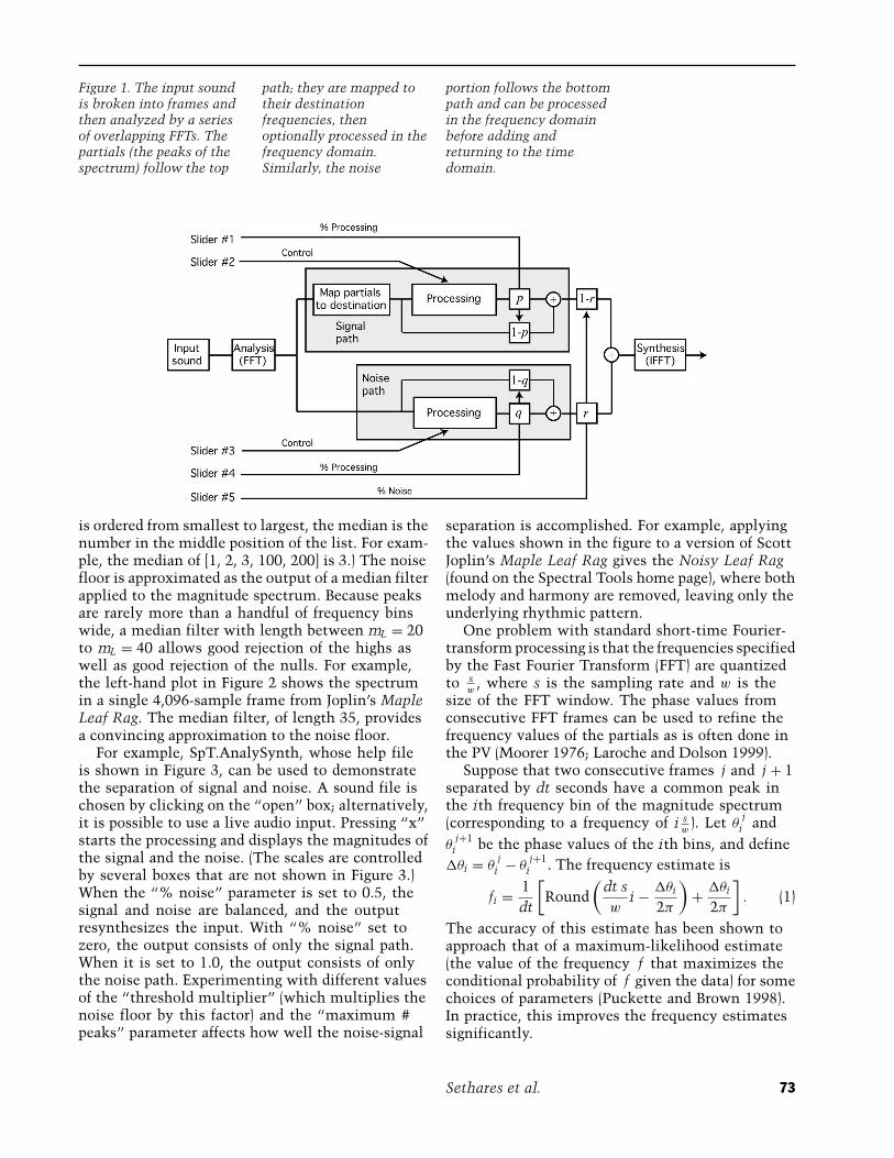
Figure 1. The input soundis broken into frames andthen analyzed by a seriesof overlapping FFTs. Thepartials (the peaks of thespectrum) follow the top

path; they are mapped totheir destinationfrequencies, thenoptionally processed in thefrequency domain.Similarly, the noise

portion follows the bottompath and can be processedin the frequency domainbefore adding andreturning to the timedomain.

is ordered from smallest to largest, the median is thenumber in the middle position of the list. For exam-ple, the median of [1, 2, 3, 100, 200] is 3.) The noisefloor is approximated as the output of a median filterapplied to the magnitude spectrum. Because peaksare rarely more than a handful of frequency binswide, a median filter with length between mL = 20to mL = 40 allows good rejection of the highs aswell as good rejection of the nulls. For example,the left-hand plot in Figure 2 shows the spectrumin a single 4,096-sample frame from Joplin’s MapleLeaf Rag. The median filter, of length 35, providesa convincing approximation to the noise floor.

For example, SpT.AnalySynth, whose help fileis shown in Figure 3, can be used to demonstratethe separation of signal and noise. A sound file ischosen by clicking on the “open” box; alternatively,it is possible to use a live audio input. Pressing “x”starts the processing and displays the magnitudes ofthe signal and the noise. (The scales are controlledby several boxes that are not shown in Figure 3.)When the “% noise” parameter is set to 0.5, thesignal and noise are balanced, and the outputresynthesizes the input. With “% noise” set tozero, the output consists of only the signal path.When it is set to 1.0, the output consists of onlythe noise path. Experimenting with different valuesof the “threshold multiplier” (which multiplies thenoise floor by this factor) and the “maximum #peaks” parameter affects how well the noise-signal

separation is accomplished. For example, applyingthe values shown in the figure to a version of ScottJoplin’s Maple Leaf Rag gives the Noisy Leaf Rag(found on the Spectral Tools home page), where bothmelody and harmony are removed, leaving only theunderlying rhythmic pattern.

One problem with standard short-time Fourier-transform processing is that the frequencies specifiedby the Fast Fourier Transform (FFT) are quantizedto s

w, where s is the sampling rate and w is the

size of the FFT window. The phase values fromconsecutive FFT frames can be used to refine thefrequency values of the partials as is often done inthe PV (Moorer 1976; Laroche and Dolson 1999).

Suppose that two consecutive frames j and j + 1separated by dt seconds have a common peak inthe ith frequency bin of the magnitude spectrum(corresponding to a frequency of i s

w). Let θ

ji and

θj+1

i be the phase values of the ith bins, and define�θi = θ

ji − θ

j+1i . The frequency estimate is

fi = 1dt

[Round

(dt sw

i − �θi

2π

)+ �θi

2π

]. (1)

The accuracy of this estimate has been shown toapproach that of a maximum-likelihood estimate(the value of the frequency f that maximizes theconditional probability of f given the data) for somechoices of parameters (Puckette and Brown 1998).In practice, this improves the frequency estimatessignificantly.

Sethares et al. 73

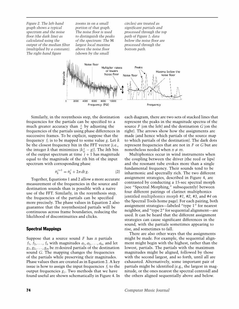
Figure 2. The left-handgraph shows a typicalspectrum and the noisefloor (the dark line) ascalculated using theoutput of the median filter(multiplied by a constant).The right-hand figure

zooms in on a smallportion of that graph.The noise floor is usedto distinguish the peaksof the spectrum: The Mlargest local maximaabove the noise floor(shown by the small

circles) are treated assignificant partials andprocessed through the toppath of Figure 1; databelow the noise floor areprocessed through thebottom path.

Similarly, in the resynthesis step, the destinationfrequencies for the partials can be specified to amuch greater accuracy than s

wby adjusting the

frequencies of the partials using phase differences insuccessive frames. To be explicit, suppose that thefrequency fi is to be mapped to some value g. Let kbe the closest frequency bin in the FFT vector (i.e.,the integer k that minimizes |k s

w− g|). The kth bin

of the output spectrum at time j + 1 has magnitudeequal to the magnitude of the ith bin of the inputspectrum with corresponding phase

θj+1

k = θj

k + 2πdt g. (2)

Together, Equations 1 and 2 allow a more accuratemeasurement of the frequencies in the source anddestination sounds than is possible with a naiveuse of the FFT. Similarly, in the resynthesis step,the frequencies of the partials can be specifiedmore precisely. The phase values in Equation 2 alsoguarantee that the resynthesized partials will becontinuous across frame boundaries, reducing thelikelihood of discontinuities and clicks.

Spectral Mappings

Suppose that a source sound F has n partialsf1, f2, . . . , fn with magnitudes a1, a2, . . . , an, and letg1, g2, . . . , gm be mdesired partials of the destinationsound G. The mapping changes the frequenciesof the partials while preserving their magnitudes.Phase values then are created as in Equation 2. A keyissue is how to assign the input frequencies fi to theoutput frequencies g j. Two methods that we havefound useful are shown schematically in Figure 4. In

each diagram, there are two sets of stacked lines thatrepresent the peaks in the magnitude spectra of thesource F (on the left) and the destination G (on theright). The arrows show how the assignments aremade (and hence which partials of the source mapto which partials of the destination). The dark dotsrepresent frequencies that are not in F or G but arenonetheless needed when n �= m.

Multiphonics occur in wind instruments whenthe coupling between the driver (the reed or lips)and the resonant tube evokes more than a singlefundamental frequency. Their sounds tend to beinharmonic and spectrally rich. The two differentassignment strategies, described in Figure 4, arecontrasted by conducting a 15-sec spectral morph(see “Spectral Morphing,” subsequently) betweenfour different pairings of clarinet multiphonics(entitled multiphonics morph #1, #2, #3, and #4 onthe Spectral Tools home page). For each pairing, bothassignment strategies—labeled “type 1” for nearestneighbor, and “type 2” for sequential alignment—areused. It can be heard that the different assignmentstrategies can cause significant differences in thesound, with the partials sometimes appearing torise, and sometimes to fall.

There are also other ways that the assignmentsmight be made. For example, the sequential align-ment might begin with the highest, rather than thelowest, partials. The partials with the maximummagnitudes might be aligned, followed by thosewith the second largest, and so forth, until all areexhausted. Alternatively, some important pair ofpartials might be identified (e.g., the largest in mag-nitude, or the ones nearest the spectral centroid) andthe others aligned sequentially above and below.

74 Computer Music Journal

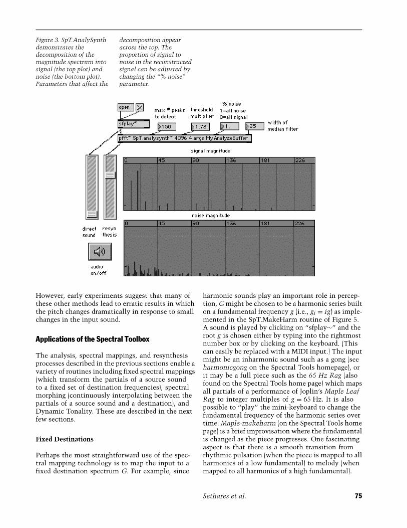
Figure 3. SpT.AnalySynthdemonstrates thedecomposition of themagnitude spectrum intosignal (the top plot) andnoise (the bottom plot).Parameters that affect the

decomposition appearacross the top. Theproportion of signal tonoise in the reconstructedsignal can be adjusted bychanging the “% noise”parameter.

However, early experiments suggest that many ofthese other methods lead to erratic results in whichthe pitch changes dramatically in response to smallchanges in the input sound.

Applications of the Spectral Toolbox

The analysis, spectral mappings, and resynthesisprocesses described in the previous sections enable avariety of routines including fixed spectral mappings(which transform the partials of a source soundto a fixed set of destination frequencies), spectralmorphing (continuously interpolating between thepartials of a source sound and a destination), andDynamic Tonality. These are described in the nextfew sections.

Fixed Destinations

Perhaps the most straightforward use of the spec-tral mapping technology is to map the input to afixed destination spectrum G. For example, since

harmonic sounds play an important role in percep-tion, G might be chosen to be a harmonic series builton a fundamental frequency g (i.e., gi = ig) as imple-mented in the SpT.MakeHarm routine of Figure 5.A sound is played by clicking on “sfplay∼” and theroot g is chosen either by typing into the rightmostnumber box or by clicking on the keyboard. (Thiscan easily be replaced with a MIDI input.) The inputmight be an inharmonic sound such as a gong (seeharmonicgong on the Spectral Tools homepage), orit may be a full piece such as the 65 Hz Rag (alsofound on the Spectral Tools home page) which mapsall partials of a performance of Joplin’s Maple LeafRag to integer multiples of g = 65 Hz. It is alsopossible to “play” the mini-keyboard to change thefundamental frequency of the harmonic series overtime. Maple-makeharm (on the Spectral Tools homepage) is a brief improvisation where the fundamentalis changed as the piece progresses. One fascinatingaspect is that there is a smooth transition fromrhythmic pulsation (when the piece is mapped to allharmonics of a low fundamental) to melody (whenmapped to all harmonics of a high fundamental).

Sethares et al. 75

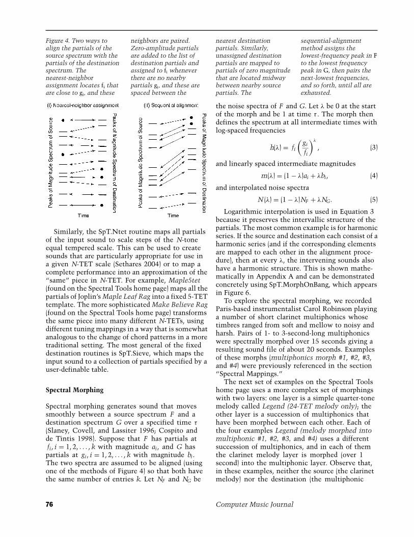
Figure 4. Two ways toalign the partials of thesource spectrum with thepartials of the destinationspectrum. Thenearest-neighborassignment locates fi thatare close to gj, and these

neighbors are paired.Zero-amplitude partialsare added to the list ofdestination partials andassigned to fi wheneverthere are no nearbypartials gj, and these arespaced between the

nearest destinationpartials. Similarly,unassigned destinationpartials are mapped topartials of zero magnitudethat are located midwaybetween nearby sourcepartials. The

sequential-alignmentmethod assigns thelowest-frequency peak in Fto the lowest frequencypeak in G, then pairs thenext-lowest frequencies,and so forth, until all areexhausted.

Similarly, the SpT.Ntet routine maps all partialsof the input sound to scale steps of the N-toneequal tempered scale. This can be used to createsounds that are particularly appropriate for use ina given N-TET scale (Sethares 2004) or to map acomplete performance into an approximation of the“same” piece in N-TET. For example, Maple5tet(found on the Spectral Tools home page) maps all thepartials of Joplin’s Maple Leaf Rag into a fixed 5-TETtemplate. The more sophisticated Make Believe Rag(found on the Spectral Tools home page) transformsthe same piece into many different N-TETs, usingdifferent tuning mappings in a way that is somewhatanalogous to the change of chord patterns in a moretraditional setting. The most general of the fixeddestination routines is SpT.Sieve, which maps theinput sound to a collection of partials specified by auser-definable table.

Spectral Morphing

Spectral morphing generates sound that movessmoothly between a source spectrum F and adestination spectrum G over a specified time τ

(Slaney, Covell, and Lassiter 1996; Cospito andde Tintis 1998). Suppose that F has partials atfi, i = 1, 2, . . . , k with magnitude ai, and G haspartials at gi, i = 1, 2, . . . , k with magnitude bi.The two spectra are assumed to be aligned (usingone of the methods of Figure 4) so that both havethe same number of entries k. Let NF and NG be

the noise spectra of F and G. Let λ be 0 at the startof the morph and be 1 at time τ . The morph thendefines the spectrum at all intermediate times withlog-spaced frequencies

h(λ) = fi

(gi

fi

)λ

, (3)

and linearly spaced intermediate magnitudes

m(λ) = (1 − λ)ai + λbi, (4)

and interpolated noise spectra

N (λ) = (1 − λ)NF + λNG. (5)

Logarithmic interpolation is used in Equation 3because it preserves the intervallic structure of thepartials. The most common example is for harmonicseries. If the source and destination each consist of aharmonic series (and if the corresponding elementsare mapped to each other in the alignment proce-dure), then at every λ, the intervening sounds alsohave a harmonic structure. This is shown mathe-matically in Appendix A and can be demonstratedconcretely using SpT.MorphOnBang, which appearsin Figure 6.

To explore the spectral morphing, we recordedParis-based instrumentalist Carol Robinson playinga number of short clarinet multiphonics whosetimbres ranged from soft and mellow to noisy andharsh. Pairs of 1- to 3-second-long multiphonicswere spectrally morphed over 15 seconds giving aresulting sound file of about 20 seconds. Examplesof these morphs (multiphonics morph #1, #2, #3,and #4) were previously referenced in the section“Spectral Mappings.”

The next set of examples on the Spectral Toolshome page uses a more complex set of morphingswith two layers: one layer is a simple quarter-tonemelody called Legend (24-TET melody only); theother layer is a succession of multiphonics thathave been morphed between each other. Each ofthe four examples Legend (melody morphed intomultiphonic #1, #2, #3, and #4) uses a differentsuccession of multiphonics, and in each of themthe clarinet melody layer is morphed (over 1second) into the multiphonic layer. Observe that,in these examples, neither the source (the clarinetmelody) nor the destination (the multiphonic

76 Computer Music Journal

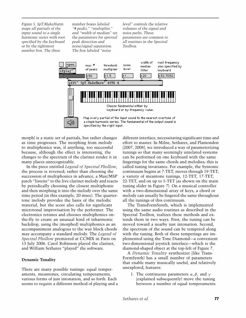
Figure 5. SpT.MakeHarmmaps all partials of theinput sound to a singleharmonic series with rootspecified by the keyboardor by the rightmostnumber box. The three

number boxes labeled“# peaks,” “multiplier,”and “width of median” setthe parameters for spectralpeak detection andnoise/signal separation.The box labeled “noise

level” controls the relativevolumes of the signal andnoise paths. Theseparameters are common toall routines in the SpectralToolbox.

morph) is a static set of partials, but rather changesas time progresses. The morphing from melodyto multiphonics was, if anything, too successfulbecause, although the effect is interesting, thechanges to the spectrum of the clarinet render it inmany places unrecognizable.

In the piece entitled Legend of Spectral Phollow,the process is reversed; rather than choosing thesuccession of multiphonics in advance, a Max/MSPpatch “listens” to the live clarinet melody and reactsby periodically choosing the closest multiphonicand then morphing it into the melody over the sametime period (in this example, 20 msec). The quarter-tone melody provides the basis of the melodicmaterial, but the score also calls for significantmicrotonal improvisation by the performer. Theelectronics retunes and chooses multiphonics on-the-fly to create an unusual kind of inharmonicbackdrop, using the (morphed) multiphonics as anaccompaniment analogous to the way block chordsmay accompany a standard melody. The Legend ofSpectral Phollow premiered at CCMIX in Paris on13 July 2006. Carol Robinson played the clarinet,and William Sethares “played” the software.

Dynamic Tonality

There are many possible tunings: equal temper-aments, meantones, circulating temperaments,various forms of just intonation, and so forth. Eachseems to require a different method of playing and a

different interface, necessitating significant time andeffort to master. In Milne, Sethares, and Plamondon(2007, 2008), we introduced a way of parameterizingtunings so that many seemingly unrelated systemscan be performed on one keyboard with the samefingerings for the same chords and melodies; this iscalled tuning invariance. For example, the Syntoniccontinuum begins at 7-TET, moves through 19-TET,a variety of meantone tunings, 12-TET, 17-TET,22-TET, and on up to 5-TET (as shown on the maintuning slider in Figure 7). On a musical controllerwith a two-dimensional array of keys, a chord ormelody can usually be fingered the same throughoutall the tunings of this continuum.

The TransFormSynth, which is implementedusing the same audio routines as described in theSpectral Toolbox, realizes these methods and ex-tends them in two ways. First, the tuning can bemoved toward a nearby just intonation. Second,the spectrum of the sound can be tempered alongwith the tuning. Both of these temperings are im-plemented using the Tone Diamond—a convenienttwo-dimensional joystick interface—which is thediamond-shaped object at the top-left of Figure 7.

A Dynamic Tonality synthesizer (like Trans-FormSynth) has a small number of parametersthat enable many musically useful, and relativelyunexplored, features:

1. The continuous parameters α, β, and γ

(explained subsequently) move the tuningbetween a number of equal temperaments

Sethares et al. 77

Figure 6. SpT.MorphOn-Bang can be applied toindividual sounds or tocomplete musicalperformances. The time

over which the morphoccurs is specified by theslider and is triggered bythe button on theright.

(e.g., 7-TET, 31-TET, 12-TET, 17-TET,and 5-TET), non-equal temperaments (e.g.,quarter-comma meantone, and Pythagorean),circulating temperaments, and closelyrelated just intonations.

2. The mapping to a two-dimensional latticeof buttons j and k on a musical controllerprovides the same fingering pattern for alltonal intervals across all possible keys andtunings within any given tuning continuum(Milne, Sethares, and Plamondon 2008).

3. The continuous parameter δ moves the tim-bre from being perfectly harmonic to beingperfectly matched to the tuning, thus mini-mizing sensory dissonance (Sethares 1993).

4. The discrete parameter c switches between anumber of different tuning continua, some ofwhich embed traditional well-formed scaleslike the pentatonic, diatonic, and chromatic(Carey and Clampitt 1989), and some ofwhich embed radically different well-formedscales (e.g., scales with three large steps andseven small steps per octave).

Each of these parameters is defined and explainedin more depth in the following subsections.

Generator Tunings (α and β) and NoteCoordinates ( j and k)

Invariant fingering over a tuning continuum re-quires a linear mapping of the notes of a higher-dimensional just intonation to the notes of a one- ortwo-dimensional temperament (such as 12-TET orquarter-comma meantone), and a linear mapping ofthese tempered notes to a two-dimensional array ofbuttons or keys on a musical controller. (The dimen-sionality of a tuning is equivalent to the minimumnumber of unique intervals (expressed in log( f ))that are required to generate, by linear combination,all of that tuning’s intervals.) Perhaps the simplestway to explain the system is by example. A p-limitjust intonation contains intervals tuned to ratiosthat can be factorized by prime numbers up to, butno higher than, p (Partch 1974). Consider 11-limitjust intonation (in which p = 11), which consistsof all the intervals generated by integer multiplesof the primes 2, 3, 5, 7, and 11. Thus simple inter-vals, such as the just fifth or just major third, canbe represented as the frequency ratios 3

2 = 2−131

and 54 = 2−251, respectively, while a less simple

interval such as the just major seventh (a perfectfifth plus a major third) is 15

8 = 2−33151. A comma

78 Computer Music Journal

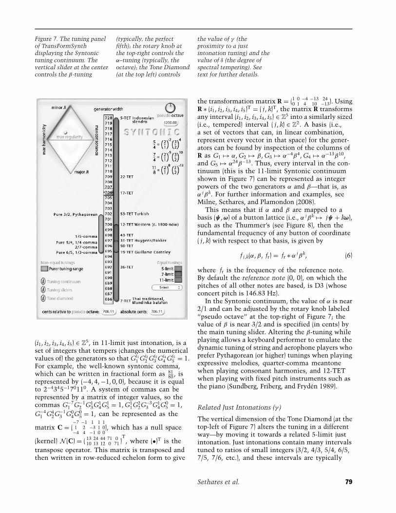
Figure 7. The tuning panelof TransFormSynthdisplaying the Syntonictuning continuum. Thevertical slider at the centercontrols the β-tuning

(typically, the perfectfifth); the rotary knob atthe top-right controls theα–tuning (typically, theoctave); the Tone Diamond(at the top left) controls

the value of γ (theproximity to a justintonation tuning) and thevalue of δ (the degree ofspectral tempering). Seetext for further details.

(i1, i2, i3, i4, i5) ∈ Z5, in 11-limit just intonation, is a

set of integers that tempers (changes the numericalvalues of) the generators so that Gi1

1 Gi22 Gi3

3 Gi44 Gi5

5 = 1.For example, the well-known syntonic comma,which can be written in fractional form as 81

80 , isrepresented by (−4, 4, −1, 0, 0), because it is equalto 2−4345−170110. A system of commas can berepresented by a matrix of integer values, so thecommas G−7

1 G−12 G1

3G14G1

5 = 1, G11G2

2G−33 G1

4G05 = 1,

G−41 G4

2G−13 G0

4G05 = 1, can be represented as the

matrix C = (−7 −1 1 1 11 2 −3 1 0

−4 4 −1 0 0), which has a null space

(kernel) N (C) = ( 13 24 44 71 010 13 12 0 71 )

T, where (•)T is the

transpose operator. This matrix is transposed andthen written in row-reduced echelon form to give

the transformation matrix R = (1 0 −4 −13 240 1 4 10 −13). Using

R ∗ (i1, i2, i3, i4, i5)T = ( j, k)T, the matrix R transformsany interval (i1, i2, i3, i4, i5) ∈ Z

5 into a similarly sized(i.e., tempered) interval ( j, k) ∈ Z

2. A basis (i.e.,a set of vectors that can, in linear combination,represent every vector in that space) for the gener-ators can be found by inspection of the columns ofR as G1 �→ α, G2 �→ β, G3 �→ α−4β4, G4 �→ α−13β10,and G5 �→ α24β−13. Thus, every interval in the con-tinuum (this is the 11-limit Syntonic continuumshown in Figure 7) can be represented as integerpowers of the two generators α and β—that is, asα jβk. For further information and examples, seeMilne, Sethares, and Plamondon (2008).

This means that if α and β are mapped to abasis (ψ , ω) of a button lattice (i.e., α jβk �→ jψ + kω),such as the Thummer’s (see Figure 8), then thefundamental frequency of any button of coordinate( j, k) with respect to that basis, is given by

f j,k(α, β, fr) = fr ∗ α jβk, (6)

where fr is the frequency of the reference note.By default the reference note (0, 0), on which thepitches of all other notes are based, is D3 (whoseconcert pitch is 146.83 Hz).

In the Syntonic continuum, the value of α is near2/1 and can be adjusted by the rotary knob labeled“pseudo octave” at the top-right of Figure 7; thevalue of β is near 3/2 and is specified (in cents) bythe main tuning slider. Altering the β-tuning whileplaying allows a keyboard performer to emulate thedynamic tuning of string and aerophone players whoprefer Pythagorean (or higher) tunings when playingexpressive melodies, quarter-comma meantonewhen playing consonant harmonies, and 12-TETwhen playing with fixed pitch instruments such asthe piano (Sundberg, Friberg, and Fryden 1989).

Related Just Intonations (γ )

The vertical dimension of the Tone Diamond (at thetop-left of Figure 7) alters the tuning in a differentway—by moving it towards a related 5-limit justintonation. Just intonations contain many intervalstuned to ratios of small integers (3/2, 4/3, 5/4, 6/5,7/5, 7/6, etc.), and these intervals are typically

Sethares et al. 79

Figure 8. The coordinates(j, k) of the Thummer’sbutton lattice, when usingits default Wicki notelayout (Milne, Sethares,and Plamondon 2008).

thought to be maximally consonant and “in tune”when using sounds with harmonic spectra. Forthis reason, just intonation has been frequentlycited as an ideal tuning (e.g., by Helmholtz 1954;Partch 1974; Mathieu 1997). However, 5-limit justintonation (JI) is three-dimensional, and higher-limitJI’s have even more dimensions, making it all butimpossible to avoid “wolf” intervals when mappingto a fixed pitch instrument (Milne, Sethares, andPlamondon 2007).

Deciding precisely which JI ratios should beused also presents a problem, because there isalways ambiguity about precisely which JI intervalis represented by a tempered interval (because themapping matrix R is many-to-one, any “reverse-mapping” is somewhat ambiguous). For this reasonwe provide two aesthetically motivated choices:“Major JI,” at the bottom of the diamond, maximizesthe number of justly tuned major triads (of ratio4:5:6); and “Minor JI,” at the top of the diamond,maximizes the number of justly tuned minor triads(of ratio 10:12:15).

The major and minor JI tuning ratios (relative tothe reference note) for every note ( j, k) are stored in atable. The major JI values are used when the controldot is in the lower half of the Tone Diamond (i.e.,sgn(γ ) = −1), the minor JI values are used when thecontrol dot is in the upper half of the Tone Diamond(i.e., sgn(γ ) = 1). Every different tuning continuumc requires a different set of values. The verticaldimension of the Tone Diamond controls how muchthe tuning is moved towards these JI values, denotedpc,sgn(γ ), j,k, using the formula ( pc,sgn(γ ), j,k

α jβk )|γ |, where

−1 ≤ γ ≤ 1 is the position of the control dot on theTone Diamond’s y-axis. This means the frequencyof any note can be calculated accordingly as

f j,k(α, β, fr, c, γ ) = fr ∗ α jβk ∗(

pc,sgn(γ ), j,k

α jβk

)|γ |. (7)

The Tone Diamond and main tuning slider, there-fore, facilitate dynamic tuning changes betweenmany different tuning systems. When the ToneDiamond’s control point is anywhere along thecentral horizontal line (the “Max. Regularity” line),the tuning is a one- or two-dimensional tuning suchas 12-TET or quarter-comma meantone, as shownon the main tuning slider. When the control pointis moved upward or downward the tuning movestowards a related just intonation. The tunings thatare intermediate between perfect regularity andJI are like the circulating temperaments of Kirn-berger and Vallotti in that every key has a (slightly)different tuning. And all of these tunings havethe same fingering when played on a 2D latticecontroller.

Spectral Tempering (δ)

The resynthesis method employed by the Trans-FormSynth enables the tuning of every partial to beindependently adjusted in real time. To make thesedynamic alterations of spectral tuning musicallyuseful, a Dynamic Tonality synthesizer can tune thepartials to be perfectly harmonic (i.e., with partialswhose frequencies are at integer multiples), temper

80 Computer Music Journal

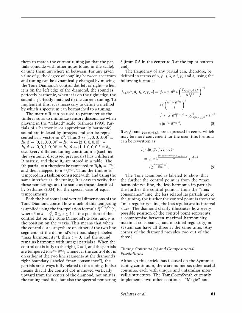
them to match the current tuning (so that the par-tials coincide with other notes found in the scale),or tune them anywhere in between. For any givenvalue of γ , the degree of coupling between spectrumand tuning can be dynamically changed by movingthe Tone Diamond’s control dot left or right—whenit is on the left edge of the diamond, the sound isperfectly harmonic; when it is on the right edge, thesound is perfectly matched to the current tuning. Toimplement this, it is necessary to define a methodby which a spectrum can be matched to a tuning.

The matrix R can be used to parameterize thetimbres so as to minimize sensory dissonance whenplaying in the “related” scale (Sethares 1993). Par-tials of a harmonic (or approximately harmonic)sound are indexed by integers and can be repre-sented as a vector in Z

5. Thus 2 ↔ (1, 0, 0, 0, 0)T ≡h2, 3 ↔ (0, 1, 0, 0, 0)T ≡ h3, 4 ↔ (2, 0, 0, 0, 0)T ≡h4, 5 ↔ (0, 0, 1, 0, 0)T ≡ h5, 6 ↔ (1, 1, 0, 0, 0)T ≡ h6,etc. Every different tuning continuum c (such asthe Syntonic, discussed previously) has a differentR matrix, and these Rc are stored in a table. Theith partial can therefore be tempered to Rchi = ( mc,i

nc,i)

and then mapped to αmc,i βnc,i . Thus the timbre istempered in a fashion consistent with (and using thesame interface as) the tuning. It is easy to verify thatthese temperings are the same as those identifiedby Sethares (2004) for the special case of equaltemperaments.

Both the horizontal and vertical dimensions of theTone Diamond control how much of this temperingis applied using the interpolation formula i( α

mc,i βnc,i

i )δ,where δ = x − |γ |

2 , 0 ≤ x ≤ 1 is the position of thecontrol dot on the Tone Diamond’s x-axis, and γ isthe position on the y-axis. This means that whenthe control dot is anywhere on either of the two linesegments at the diamond’s left boundary (labeled“max harmonicity”), then δ = 0, and the soundremains harmonic with integer partials i. When thecontrol dot is fully to the right, δ = 1, and the partialsare tempered to αmc,i βnc,i ; whenever the control dot ison either of the two line segments at the diamond’sright boundary (labeled “max consonance”), thepartials are always fully related to the tuning. It alsomeans that if the control dot is moved verticallyupward from the center of the diamond, not only isthe tuning modified, but also the spectral tempering

δ (from 0.5 in the center to 0 at the top or bottomend).

The frequency of any partial can, therefore, bedefined in terms of α, β, j, k, c, i, γ , and δ, using thefollowing formula:

fi, j,k(α, β, fr, c, γ , δ) = fr ∗ α jβk ∗(

pc,sgn(γ ), j,k

α jβk

)|γ |

∗ i(

αmc,i βnc,i

i

)δ

= fr ∗ (α jβk)1−|γ | ∗ p|γ |c,sgn(γ ), j,k ∗ i1−δ

∗ (αmc,i βnc,i )δ. (8)

If α, β, and pc,sgn(γ ), j,k, are expressed in cents, whichmay be more convenient for the user, this formulacan be rewritten as

fi, j,k(α, β, fr, c, γ , δ)

= fr ∗ 2(1−|γ |)( jα+kβ)+|γ |pc,sgn(γ ), j,k

1200 ∗ i1−δ

∗ 2δ(αmc,i+βnc,i )

1200 . (9)

The Tone Diamond is labeled to show thatthe further the control point is from the “maxharmonicity” line, the less harmonic its partials;the further the control point is from the “maxconsonance” line, the less related its partials are tothe tuning; the further the control point is from the“max regularity” line, the less regular are its intervalsizes. The diamond clearly illustrates how everypossible position of the control point representsa compromise between maximal harmonicity,maximal consonance, and maximal regularity; nosystem can have all three at the same time. (Anycorner of the diamond provides two out of thethree.)

Tuning Continua (c) and CompositionalPossibilities

Although this article has focused on the Syntonictuning continuum, there are numerous other usefulcontinua, each with unique and unfamiliar inter-vallic structures. The TransFormSynth currentlyimplements two other continua—”Magic” and

Sethares et al. 81

“Hanson” (Erlich 2006)—which open up interestingcompositional avenues. They contain scales thatembed numerous major and minor triads, but thesescales have a radically different structure than thosefound in any standard Western tuning. For example,the Magic continuum has a ten-note well-formedscale (with seven small steps and three large steps)that contains ten major or minor triads; the Hansoncontinuum has an eleven-note well-formed scale(with seven small steps and four large steps) thatalso contains ten major or minor triads. MagicTraveller (found on the Spectral Tools home page)uses this Magic scale. It may well be that the chordsin these systems have functional relationships thatare quite different from those found in standarddiatonic/chromatic harmony. Such systems, there-fore, open up the possibility of an aesthetic researchprogram similar to that which may be said to havecharacterized the development of common-practicemusic from the rise of functional harmony in theseventeenth century to the “crisis of tonality” atthe end of the nineteenth.

But the well-structured tonal relationships foundin these continua do not support only a strictly tonalcompositional style. Serial (and other “atonal”) com-positional techniques are just as applicable to thesealternative continua, as are techniques that explorethe implications of unusual timbral combinationsand structures. Each continuum offers a unique setof mathematical possibilities and constraints. Forexample, the familiar 12-note division of the octaveincludes many factors (2, 3, 4, and 6), thus enablinginterval classes of these sizes to cycle back to thestarting note, and modes of limited transpositionto be formed (Messiaen 1944). Conversely, a 13-notedivision of the octave, which can be made to soundquite “in-tune” when the spectrum is tempered tothe Magic continuum, has no factors and so containsno modes of limited transposition and no intervalcycles. The 15-note division found in Hanson hasfactors of 3 and 5, suggesting a quite different set ofstructural possibilities. ChatterBar and Lighthouse(found on the Spectral Tools homepage) are bothnon-serial “atonal” pieces—in 53-TET Syntonic and11-TET Hanson, respectively.

Alongside these structural possibilities are thedynamic variations in tuning and timbre that can

be easily controlled (and even notated) with the α,β, γ , and δ parameters. Smooth changes of tuningand timbre are at the core of C2ShiningC, while inShred (found on the Spectral Tools home page), themusic switches from 12-TET to 5-TET Syntonic.We believe Dynamic tonality offers a rich setof compositional possibilities of both depth andsimplicity.

Discussion

The analysis–resynthesis method used by theSpectral Toolbox allows the independent controlof both frequency and amplitude for every partialin a given sound. However, because a typicalmusical sound consists of tens or even hundreds ofaudible partials, it is apparent that their individualmanipulation is not necessarily practical. To reduceinformation load and retain musical relevance,there is need for an organizational routine thatparameterizes spectral information in a simpleand musically meaningful interface. The SpectralToolbox has addressed this problem by providingthree different routines: (1) mapping partials to afixed destination, (2) morphing between differentspectra, and (3) Dynamic Tonality.

Although we have so far only discussed thereconstruction of preexisting sounds, it is also pos-sible to manipulate the harmonic information ofpurely synthesized sound. The ideas presented inthis article are applicable to virtually any synthesismethod that allows complete control over harmonicinformation. For example, The Viking (Milne andPrechtl 2008) is an additive synthesizer that imple-ments Dynamic Tonality in the same manner as theTransFormSynth, except that it synthesizes eachpartial with its own sinusoidal oscillator. Similarly,2032 (available on the Dynamic Tonality Web site)is a modal synthesizer that implements DynamicTonality in a physical-modeling algorithm. In thiscase, an excitation signal is fed through a seriesof resonant filters that represent specific partialsthrough their individual feedback coefficients.

There are benefits pertaining to each of thesesynthesis methods: Additive synthesis is, relativelyspeaking, computationally efficient, whereas modal

82 Computer Music Journal

synthesis, at the cost of greater computationalpower, enables realistic and dynamic physical mod-eling. However, the analysis–resynthesis method isinteresting because it enables the harmonic manip-ulation of any sound, and it can do so for both fixedand live audio inputs. This means that, given its rel-atively simple user interface, the Spectral Toolboxhas the capacity to provide novel and worthwhileapproaches to computer-music composition andperformance. The musical examples available onthe Web site are intended to illustrate some of theseartistic possibilities.

Beyond the artistic benefits described herein, thiswork also provides strong implications for musicresearch, particularly in the area of cognition. Themutual control of tuning and timbre facilitates adeeper examination of the musical ramificationsthat such a relationship entails. Perhaps of greatestinterest is how formerly inaccessible (that is, in anaesthetic sense) tunings can be rendered accessiblethrough the timbral manipulations described inthis article. Such an idea calls for further researchregarding varying forms of dissonance—most no-tably melodic dissonance (Van der Merwe 1992;Weisethaunet 2001)—and harmonic tonality in gen-eral. Such concepts can now take alternative tuningsinto account. Tools such as the Spectral Toolbox canfacilitate a wider use of microtonality in electro-acoustic composition, performance, and research.

Acknowledgments

The authors would like to thank Gerard Pape forhelpful discussions and Carol Robinson for theexcellent performance of Legend.

References

Carey, N., and D. Clampitt. 1989. “Aspects of Well-Formed Scales.” Music Theory Spectrum 11:187–206.

Carlos, W. 1987a. “Tuning: At the Crossroads.” ComputerMusic Journal 11(1):29–43.

Carlos, W. 1987b. Secrets of Synthesis. Audio compactdisc. East Side Digital ESD 81702.

Cospito, G., and R. de Tintis. 1998. “Morph: Timbre Hy-bridization Tools Based on Frequency Domain Process-ing.” Paper presented at the 1998 Workshop on DigitalAudio Effects (DAFx-98), Barcelona, 21 November.

Dolson, M. 1986. “The Phase Vocoder: A Tutorial.”Computer Music Journal 10(4):14–27.

Erlich, P. 2006. “A Middle Path Between Just Intonationand the Equal Temperaments, Part 1.” Xenharmonikon18:159–199.

Helmholtz, H. L. F. 1954. On the Sensations of Tone.New York: Dover.

Keislar, D. 1987. “History and Principles of MicrotonalKeyboards.” Computer Music Journal 11(1):18–28.Published with corrections in 1988 as “History andPrinciples of Microtonal Keyboard Design,” ReportSTAN-M-45, Stanford University. Available onlineat ccrma.stanford.edu/STANM/stanms/stanm45/.(Accessed 30 December 2008.)

Laroche, J., and M. Dolson. 1999. “Improved PhaseVocoder Time-Scale Modification of Audio.” IEEETransactions on Audio and Speech Processing 7(3): 323–332.

Lyon, E. 2004. “Spectral Tuning.” Proceedings of the2004 International Computer Music Conference. SanFrancisco: International Computer Music Association,pp. 375–377.

Mathieu, W. A. 1997. Harmonic Experience. Rochester:Inner Traditions.

Messiaen, O. 1944. Technique de mon langage musical.Paris: Leduc.

Milne, A. J., and A. Prechtl. 2008. “New Tonalities withthe Thummer and The Viking.” Paper presented at theThird International Haptic and Auditory InteractionDesign Workshop. Jyvaskyla, Finland: University ofJyvaskyla, pp. 20–22.

Milne, A. J., W. A. Sethares, and J. Plamondon. 2007.“Isomorphic Controllers and Dynamic Tuning:Invariant Fingering over a Tuning Continuum.”Computer Music Journal 31(4):15–32.

Milne, A. J., W. A. Sethares, and J. Plamondon. 2008.“Tuning Continua and Keyboard Layouts.” Journal ofMathematics and Music 2(1):1–19.

Moorer, J. A. 1976. “The Use of the Phase Vocoder inComputer Music Applications.” Journal of the AudioEngineering Society 26(1/2):42–45.

Partch, H. 1974. Genesis of a Music. New York: Da CapoPress.

Puckette, M. S., and J. C. Brown. 1998. “Accuracyof Frequency Estimates Using the Phase Vocoder.”IEEE Transactions on Speech and Audio Processing6(2):166–176.

Sethares et al. 83

Serra, X., and J. Smith. 1990. “Spectral ModelingSynthesis: A Sound Analysis/Synthesis System Basedon a Deterministic Plus Stochastic Decomposition.”Computer Music Journal 14(4):12–24.

Sethares, W. A. 1993. “Local Consonance and theRelationship between Timbre and Scale.” Journal ofthe Acoustical Society of America 94(3):1218–1228.

Sethares, W. A. 1998. “Consonance-Based SpectralMappings.” Computer Music Journal 22(1):56–72.

Sethares, W. A. 2004. Tuning, Timbre, Spectrum, Scale,2nd ed. London: Springer-Verlag.

Slaney, M., M. Covell, and B. Lassiter. 1996. “AutomaticAudio Morphing.” Proceedings of the 1996 ICASSP,Atlanta, GA.

Sundberg, J., A. Friberg, and L. Fryden. 1989. “Rulesfor Automated Performance of Ensemble Music.”Contemporary Music Review 3(1):89–109.

Van der Merwe, P. 1992. Origins of the Popular Style.Oxford: Clarendon Press.

Weisethaunet, H. 2001. “Is There Such a Thing as the‘Blue Note’?” Popular Music 20(1):99–116.

Appendix: Preservation of Intervallic StructureUnder Logarithmic Interpolation

Suppose that the n source peaks fi and the ndestination peaks gi have the same intervallicstructure, i.e., that

fi+1

fi= gi+1

gi(10)

for i = 1, 2, . . . , n − 1. Morphing the two soundsusing the logarithmic method (Equation 3) creates acollection of intermediate sounds with peaks at

hi(λ) = fi

(gi

fi

)λ

. (11)

Then, for every 0 ≤ λ ≤ 1, the intervallic structurein the hi(λ) is the same as that in the source anddestination. To see this, observe that

hi+1(λ)hi(λ)

=fi+1

(gi+1fi+1

)λ

fi(

gifi

)λ= fi+1

fi

(gi+1

fi+1

)λ (figi

)λ

= fi+1

fi

(gi+1

gi

fifi+1

)λ

= fi+1

fi(12)

The last equality follows directly from Equation10. In particular, if the fi and gi are the n partialsof harmonic sounds (though perhaps with differentmagnitudes and different fundamentals) then theinterpolated sounds h(λ) are also harmonic, withspectra that smoothly connect f and g and withfundamental frequency (and hence, most likely,with pitch) that moves smoothly from that of f tothat of g.

84 Computer Music Journal