spectrallyefﬁcientcommunicationovertime-varying … · quality of service ... while maintaining...

Hindawi Publishing CorporationEURASIP Journal on Applied Signal ProcessingVolume 2006, Article ID 35352, Pages 1–16DOI 10.1155/ASP/2006/35352

Spectrally Efficient Communication over Time-VaryingFrequency-Selective Mobile Channels: Variable-SizeBurst Construction and Adaptive Modulation

Francis Minhthang Bui and Dimitrios Hatzinakos

The Edward S. Rogers Sr. Department of Electrical and Computer Engineering, University of Toronto,10 King’s College Road, Toronto, ON, Canada M5S 3G4

Received 1 June 2005; Revised 10 March 2006; Accepted 15 March 2006

Methods for providing good spectral efficiency, without disadvantaging the delivered quality of service (QoS), in time-varyingfading channels are presented. The key idea is to allocate system resources according to the encountered channel. Two approachesare examined: variable-size burst construction, and adaptive modulation. The first approach adapts the burst size according tothe channel rate of change. In doing so, the available training symbols are efficiently utilized. The second adaptation approachtracks the operating channel quality, so that the most efficient modulation mode can be invoked while guaranteeing a target QoS.It is shown that these two methods can be effectively combined in a common framework for improving system efficiency, whileguaranteeing good QoS. The proposed framework is especially applicable to multistate channels, in which at least one state canbe considered sufficiently slowly varying. For such environments, the obtained simulation results demonstrate improved systemperformance and spectral efficiency.

Copyright © 2006 Hindawi Publishing Corporation. All rights reserved.

1. INTRODUCTION

Achieving high spectral efficiency is an important goal incommunication. However, it is equally important that thequality of service (QoS), quantified by the bit error rate(BER), will not deteriorate as a result of this goal. We proposestrategies that allocate resources for improving the spectralefficiency, while maintaining good QoS, for burst-by-burstcommunication systems. In these systems, data are transmit-ted in bursts or blocks, possibly with training and other typesof symbols to aid data recovery at the receiver. Over any suchburst, the channel is assumed to be sufficiently constant orstationary, that is, a single channel environment is approxi-mately experienced by the entire data burst (also known as aquasi-static or block-fading channel). The rationale for em-ploying burst transmission is that since the channel is ap-proximately the same over the entire received burst, it can beestimated, and a single time-invariant equalizer can be usedto mitigate interferences for all data symbols within a singleburst. In other words, the various data bursts can be indepen-dently processed at the receiver, on a burst-by-burst basis.

Unfortunately, with the advent of the systems employ-ing high-frequency carriers and used in high-speed envi-ronments, the quasi-static channel assumption is becomingmore questionable. Essentially, the channel can be regarded

as constant over a burst if the burst duration is less than thechannel coherence time TC . However, the channel coherencetime is itself actually a statistical measure, whose precise for-mula depends on the definition criterion. Loosely speaking,[1, 2],

TC ≈ 1fm

(1)

or alternatively, defined as the time over which the time cor-relation function is above 0.5 [1, 2],

TC ≈ 916π fm

, (2)

where fm is the maximum Doppler shift given by

fm = vmλ= vm fc

c(3)

with vm being the mobile speed, λ the wavelength, fc the car-rier frequency, and c the speed of light. The relationship withthe burst duration can also be viewed using the normalizedDoppler shift fmTS, where TS is the symbol duration. Then,using (1), a burst is within a coherence time if the number ofsymbols in the burst, that is, the burst size BS, is

BS <1

fmTS. (4)

2 EURASIP Journal on Applied Signal Processing

20

10

0

−10−20−30−40R

eceivedenvelope(dB)

0 1 2 3 4 5 6 7 8×104Data symbol

(a)

20

0

−20−40−60R

eceivedenvelope(dB)

0 1 2 3 4 5 6 7 8×104Data symbol

(b)

Figure 1: Received envelopes over fading channels at carrier frequency fc = 3.5GHz: (a) mobile speed vm = 100 km/h, or normalizedmaximum Doppler shift fmTS = 5.55× 10−4; (b) vm = 10 km/h, or fmTS = 5.55× 10−5.

Regardless of which definition, (1) or (2), is used, the co-herence time TC is inversely proportional to the both car-rier frequency fc and the mobile speed vm. Hence, with anincrease of the carrier frequency fc in modern systems, TC

tends to become shorter. In practice, the burst duration ischosen to be significantly less than TC in order to justifythe quasi-static assumption. For example, in GSM [1, 2], aburst duration is 0.577ms, while TC ≈ 11ms (using (1) withfc = 960MHz, v = 100 km/h).

With an increased carrier frequency, for example, fc < 3.5GHz in the developing IEEE802.20 standard, the coherencetime reduces to TC ≈ 3.6ms, and with target bitrates on theorder of 1Mbps, the symbol duration TS ≈ 2μs (assuming2 bits/symbol, e.g., using 4-QAM [2, 3]). Hence, the normal-ized Doppler shift is fmTS ≈ 5.55 × 10−4, and a coherencetime contains at a maximum 1/( fmTS) = 1800 symbols.

For visualization purposes, Figure 1 shows typical fadingenvelopes versus the symbol index for the above calculatednormalized Doppler shift fmTs ≈ 5.55 × 10−4, and also forfmTs ≈ 5.55 × 10−5. Here, the time variations are describedby the Jakes power spectral density (see (7)). The smaller nor-malized Doppler shift corresponds to a more slowly varyingchannel.

In coping with the reduced coherence time TC , a num-ber of approaches can be considered. First, the channel in-variance assumption can be eliminated, and new receiverstructures can be designed. However, suppose that suchchanges are not permissible, for example, due to existinginfrastructure or hardware constraints. Then, the question iswhether basic burst-by-burst techniques can still be used inrapidly time-varying channels. We examine techniques forachieving reliable communications in such channels, while

still using the same basic burst-by-burst receiver methodol-ogy.

Ultimately the goal is to shorten the burst duration insome manner, so that it remains within the coherence dura-tion. Following are example methods that can be considered.

(S1) Reduce the number of data symbols per burst

To reduce the overall burst duration, the symbol durationTS must not be increased. With this solution, the transmis-sion efficiency, that is, the ratio of useful data symbols overall symbols in a burst, can be severely affected, especially inrapidly varying channels.

(S2) Reduce the burst duration

Alternatively, the same number of symbols in a burst can bemaintained, but the symbol duration TS is reduced. Whilethe transmission efficiency is maintained, if the symbol du-ration is too short relatively to the channel delay spread, thechannel becomes highly frequency selective, with severe in-tersymbol interference (ISI). The use of a high-complexityequalizer would be needed for acceptable QoS.

(S3) Use a variable-size burst approach

A key bottleneck in the previous two methods is the assump-tion of a fixed-size burst, chosen to satisfy the worst casescenario. This is inefficient when the encountered channel isslowly changing, for example, when the mobile speed is low.The idea of a variable-size burst [4] is to use a shorter burstwhen the channel is changing quickly. Conversely, durations

F. M. Bui and D. Hatzinakos 3

over which the channel is slowly changing will be exploitedto use a larger burst. As will be seen in Section 3, this enablesa better use of the available training symbols for improvedtransmission efficiency and QoS. Moreover this constructioncan be achieved entirely at the receiver.

If the channel quality is further known for each burst, itis also possible to adapt the modulation mode for the datasymbols on a burst-by-burst basis. When the channel is be-nign or of good quality, a higher-order modulation constel-lation, for example, 16-QAM, can be used for efficiency whilestill maintaining a good QoS, defined by a target BER. How-ever, when the channel is hostile or of poor quality, a lower-order modulation mode, for example, BPSK, is selected tomaintain an acceptable QoS. Known as adaptive modula-tion [3, 5], this methodology permits an overall improve-ment in spectral efficiency. Thus, adaptive modulation playsa key role in balancing the system’s integrity and efficiency ina time-varying environment.

As will become evident in the remainder of the paper,the overall conclusion of this work is the following: if theunderlying time-varying channel can be modeled as multi-state, where at least one state is slowly varying, then reliablecommunication is still possible using conventional burst-by-burst techniques when coupled with a variable-size burst ap-proach. Furthermore, the spectral efficiency can be enhancedwith the use of adaptive modulation. When combined to-gether, these two strategies deliver an attractive framework,with minimal modifications of existing systems, for reliableand efficient communication over time-varying channels.

When there is no slow state in the underlying channel,the transmission efficiency is poor since the burst size needsto be very small. By combining variable-size burst construc-tion with basis-expansion modeling (BEM) of the channel[6, 7], the transmission efficiency can be improved. However,in this case, the system complexity is increased due to morecomplicated estimation and equalization procedures. Withsome performance loss, the complexity can be reduced sig-nificantly using time-varying FIR equalization [8]. But moreimportantly, even with the addition of basis-expansion mod-eling, the variable-size burst methodology remains applica-ble [6]. This is because, under certain conditions, BEM es-sentially allows a rapidly varying channel to be treated as anequivalent slow fading channel. In fact, at the cost of systemcomplexity, the BEM modification only improves the flexi-bility of variable-size burst construction, making it applica-ble to a wider range of time-varying channels [6]. In the in-terest of brevity and clarity, this work will thus focus on burstconstruction, and the integration with adaptive modulation,all using conventional channel modeling.

The rest of this paper is organized as follows. After de-scribing a mobile channel model with multistate consider-ations in Section 2, a variable-size burst structure is pre-sented in Section 3. Channel equalization technique and es-timation techniques are then outlined in Section 4. Thesetechniques are subsequently incorporated into a channel-tracking framework for constructing variable-size bursts inSection 5. And to further improve the spectral efficiency,an adaptive modulation method coupled with variable-size

burst construction is discussed in Section 6. Next, to demon-strate the performance of the proposed methods, simulationresults are obtained in Section 7. Lastly, conclusions aremadein Section 8.

2. CHANNELMODEL

2.1. Mobile fading channels

In this paper, time-varying frequency-selective mobile fadingchannels are assumed. Under the well-known wide-sense sta-tionary uncorrelated scatterers, (WSSUS) assumptions [2, 9],such channels can be viewed as equivalent time-varying FIRfilters, with impulse response

h(t, τ) =P−1∑

p=0αp(t)δ

(τ − τp

), (5)

where P is the number of observable paths, as will as τp andαp(t), respectively, the delay and gain of the pth path.

The time variations, due to the Doppler effect as men-tioned in Section 1, are described for each of the P paths bythe autocorrelation function [9]:

rp(τ) = σ2pJ0(2π fmτ

)(6)

or, equivalently, in the frequency domain, by the Jakes powerspectral density:

Sp( f ) =

⎧⎪⎪⎪⎨⎪⎪⎪⎩

σ2p

π fm√1− ( f / fm

)2 , | f | < fm,

0, | f | > fm,

(7)

where σ2p is the average power of the pth path, J0(·) the zero-order Bessel function of the first kind, and fm the maximumDoppler shift. Note that the coherence time TC from (2) isdefined based on (6).

The channel frequency selectivity is described by specify-ing the average power for each of the path coefficients αp(t),resulting in the power-delay profile. For example, a typicalurban (TU) COST207-type [3, 9] channel power-delay pro-file with four observable paths is shown in Figure 2, with pa-rameters summarized in Table 1.

2.2. Multistate extension

While the above mobile channel model is both time and fre-quency selective, it essentially describes one single channelstate or environment, where a state is characterized by a par-ticular fm. From Section 1, fm is dependent on the mobilevelocity vm for a fixed carrier frequency fc. Hence, as a userchanges his or her mobile activities, the perceived operatingenvironment is also effectively modified. In the context of avariable-size burst, it is beneficial to model such activitiesexplicitly, since the goal is to exploit low-mobility activitiesfor efficiency. To this end, we consider a multistate channelmodel, where each state is defined by an associated Dopplershift fm or mobile speed vm. Evidently, the more states con-sidered, the more accurate is the approximation of the user’smobile activities, at the cost of complexity.


0.8

0.7

0.6

0.5

0.4

0.3

0.2

0.1

0

Normalized

path

power

0 0.5 1 1.5 2 2.5 3 3.5 4

Path delay (μs)

Figure 2: Normalized power-delay profile for a 4-path typical ur-ban (TU) COST207-type channel, with parameters summarized inTable 1.

Table 1: Normalized power-delay profile for a typical urban (TU)COST207-type channel, as depicted in Figure 2.

Delay position (μs) Path power0 0.7236

1.54 0.15542.31 0.07202.69 0.0490

Suppose the user’s mobile activities are such that thereare κ distinguishable states: {k1, k2, . . . , kκ}. Denote the prob-ability of the user being in the ki state as p(ki), so that

κ∑

i=1p(ki) = 1. (8)

To fully describe the user’s mobile behavior as a functionof time, the joint probability mass function (pmf) needs tobe specified as a function of the current state, and the paststate(s), that is, memory consideration. However, for sim-plicity, we assume in this paper a memoryless model. Then,the channel states for various time instants can be considereddiscrete i.i.d random variables, with the pmf specified by

p(ki), i = 1, . . . , κ. (9)

Note that when considering a quasi-static channel approxi-mation, the probability of the channel for any burst being ina certain state is specified by (9), that is, on a burst-by-burstbasis.

2.3. A Two-state channel example

As an example of a channel with two states, when using aGauss-Markov approximation to the Jakes model, considerthe following composite Gauss-Markov channel, used previ-ously in [4]. Denote the channel taps for the nth time instant

20

10

0

−10−20−30−40R

eceivedenvelope(dB)

0 400 800 1200 1600 2000 2400

Data symbol

(a)

10

0

−10−20−30−40R

eceivedenvelope(dB)

0 400 800 1200 1600 2000 2400

Data symbol

(b)

Figure 3: Quasi-static channel approximation for fmTS = 1× 10−3

using: (a) fixed-size bursts of 100 symbols; (b) fixed-size bursts of400 symbols.

as hn. Let the two states be s-state and f -state. Then the chan-nel changes between time instants as

hn = ν(ηs hn−1 + us

)+(1− ν

)(η f hn−1 + u f

), (10)

where ν is a Bernoulli random variable, ηs, η f the correlationcoefficients for each state, and us, u f the noise terms. Hence,by appropriately assigning values to ηs and η f , the channelcan be considered as composing of a slow and a fast state,with state probabilities specified by the Bernoulli rv ν.

For the above composite Gauss-Markovmodel, each stateis specified by parameters relating to the associated Dopplershift fm, for example, s-state by ηs. In this paper, each channelstate is described more generally using (6) and (7).

3. VARIABLE-SIZE BURST STRUCTURE

A variable-size burst structure, based on a conventionalfixed-size burst, is described in this section.

3.1. Motivation

As mentioned in Section 1, the idea of using a burst trans-mission system originates from approximating the channel asconstant or quasi-static over some interval, which should beless than the coherence time. In the context of a time-varyingmobile channel, Figure 3 illustrates this approximation ona channel with normalized Doppler shift fmTS = 1 × 10−3

for two different fixed-size bursts: (a) a smaller burst of 100data symbols; and (b) a larger burst of 400 data symbols. Forthis scenario, the smaller burst approximates more accurately


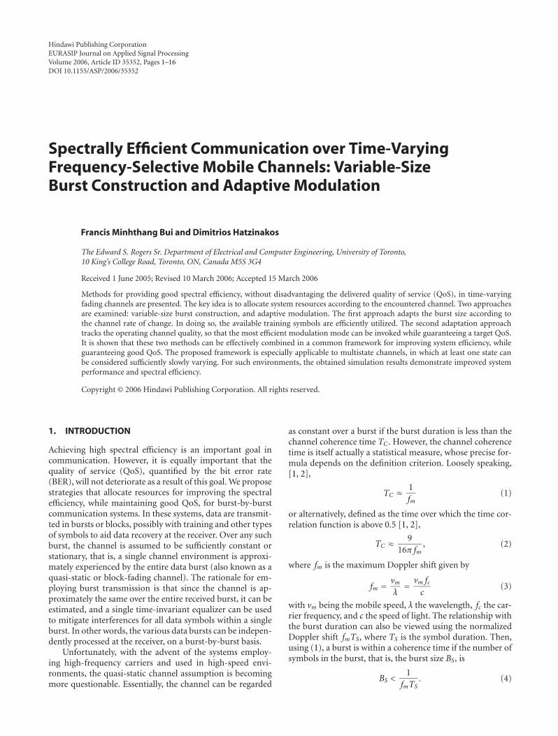
Training Data Guard interval

G1 G2 = G3 G4 = G5 = G6 G7 = G8

H1 H2 H3 H4

(a)

Transmittedburst

Receivedburst

(b)

Receivedburst

Receivedburst

Receivedburst

Receivedburst

(c)

Figure 4: Variable-size burst structure with preamble training sym-bols: (a) quasi-static channel approximations for each burst, wheresome channels may be the same, for example, G2 = G3 ≡ H2;(b) fixed-size burst system, assuming all channels are different; (c)variable-size (received) burst system, exploiting knowledge of chan-nel similarities.

the channel using a total of 24 fixed data bursts. The largerburst approximates the same channel using fewer data bursts,a total of 6 in this case. With a fixed overhead of train-ing symbols per burst, it is more desirable to use the largerburst, since the transmission efficiency (which is propor-tional to the spectral efficiency) would be higher. However, asillustrated by Figure 3(b), the larger-burst approximation isquite inaccurate at certain times, for example, the deep fadearound symbol 1000 is missed entirely. On the other hand,the smaller burst is rather redundant at certain times, for ex-ample, over the symbol range 1200–1500, a single-burst ap-proximation suffices. Hence, a compromise between the twodifferent burst sizes, using a variable-size burst, is advanta-geous in terms of efficiency.

3.2. Accumulated received burst structure

Figure 4 shows a potential variable-size burst structure. Thekey idea here is to realize the distinction between a transmit-ted and a received burst: regardless of what the transmittersends, the receiver ultimately can make a choice on what itconsiders a received burst (used for further processing, suchas channel estimation). Then, the transmitter simply trans-mits fixed-size fundamental bursts. At the receiver, a variable-size burst is constructed by combining consecutive trans-mitted fundamental bursts appropriately. For this scheme tofunction, as in a fixed-size burst system, the fundamentalbursts need to satisfy the quasi-static channel conditions. Thedifference is that, by tracking the channel, the receiver can de-tect a slowly changing duration, and accordingly adapts theburst size by combining the consecutive fundamental bursts

within this duration. The result is a larger accumulated burst,composed of fundamental bursts, with an enlarged set oftraining symbols delivering a more accurate channel estima-tion.

3.3. Example construction

To illustrate the described procedure, Figure 4(a) shows anexample scenario, where the channels for eight consecutivefundamental bursts are designated: G1,G2, . . . ,G8. A fixed-size burst receiver simply assumes that these channels are alldifferent and constructs received bursts of the same size asthe transmitted bursts as shown in Figure 4(b). However, ifthe underlying channels are not all different, then a variable-size burst can combine appropriate consecutive fundamentalbursts to form larger accumulated bursts, while still satisfyingthe quasi-static assumption. For example, if G2 = G3, G4 =G5 = G6, G7 = G8 (see Figure 3, e.g., of how this may arise),then the unique channels can be re-designated asH1,H2,H3,H4, from which there would be four enlarged variable-sizeaccumulated bursts as in Figure 4(c).

3.4. Comparisons to a fixed-size burst

From a transmitter perspective, there is essentially no differ-ence in terms of the burst structure. The fundamental burstsize is still specified by the highest-speed fm. However, inrapidly time-varying channels, the variable-size burst struc-ture is more attractive, because it has the potential to main-tain good spectral efficiency.

Indeed, consider using solution (S1), from Section 1, toreduce the number of data symbols per burst. Then, to main-tain the same transmission efficiency, the number of train-ing symbols must also be reduced. However, estimation andequalization depend on the raw number of training sym-bols (and not the transmission efficiency). Hence, a fixed-size burst, which in general has insufficient training symbolsin rapidly time-varying channels, will suffer from significantperformance degradation due to unsuccessful channel esti-mation and equalization. By contrast, a variable-size bursthas the potential to regain the performance loss by makingthe best use of the available training symbols.

The effect of training-symbol assignment or placement isnot investigated here. While optimal training placement canhave a significant impact on the overall performance [10],the present paper has a different perspective: given a train-ing regime (e.g., preamble, midamble, or superimposed), theproblem is how to combine the available training symbolsfrom different bursts in an advantageous manner, notablyby tracking the channel. This is based on the assumptionthat more training symbols would yield better overall per-formance.

4. CHANNEL EQUALIZATION AND ESTIMATION

The proposed variable-size burst scheme requires the re-ceiver to correctly detect the channel changes. Such channel-tracking capability is designed by modifying conventionalquasi-static channel equalization and estimation techniques.


First, we will describe the ideal minimum mean-square(MMSE) equalizer, assuming knowledge of the channel.Then, using training symbols, a maximum-likelihood (ML)estimator provides an estimate of the channel. Through-out this section, it is assumed that the accumulated burstis already received under quasi-static channel conditions.In Section 5, the channel estimation and equalization tech-niques described here will be incorporated in a frameworkfor constructing a quasi-static accumulated burst.

4.1. MMSE equalization

Consider the typical equivalent baseband signal representa-tion

y[n] =L−1∑

l=0h[n; l]x[n− l] + v[n], (11)

where x[n] is the transmitted symbol at instant n, y[n]the received symbol, h[n; l] the channel impulse response, Lthe channel length (assumed known), and v[n] the additivewhite Gaussian noise (AWGN) with variance σ2v . When thechannel is time invariant as in a burst-by-burst system, thedependence of h[n; l] on n is suppressed:

y[n] =L−1∑

l=0h[l]x[n− l] + v[n] = h[n]� x[n] + v[n], (12)

where� denotes convolution. In this case, a matrix formula-tion can be obtained. At the instant n, for the potential recov-ery of the nth symbol x[n], N consecutive received symbolsare collected as

y(n) = Hx(n) + v(n) (13)

with y[n] = [y[n], . . . , y[n−N+1]]T , v[n] = [v[n], . . . , v[n−N + 1]]T , x[n] = [x[n], . . . , x[n−N − L + 2]]T ,

H =

⎡⎢⎢⎢⎢⎣

h[0] · · · h[L− 1] · · · 0

. . .

0 · · · h[0] · · · h[L− 1]

⎤⎥⎥⎥⎥⎦, (14)

where (·)T denotes matrix transpose, and H has dimensionsN × (N + L− 1).

Using the minimum mean-squared error (MMSE) cri-terion, a linear equalizer f = [ f [0], f [1], . . . , f [N − 1]]T isfound by minimizing the cost function

JMSE(f) = E(∣∣fHy(n)− x[n− δ]

∣∣2), (15)

where E(·) denotes the expectation operator, (·)H the Her-mitian transpose, and δ is a delay, with permissible valuesδ = 0, . . . ,N + L − 1 (see (18) and (19) for the effect of δ).The solution to (15) is [11]

f = R−1p, (16)

where R = E(y(n)yH(n)), p = E(x∗[n− δ]y(n)) are known,respectively, as the autocorrelation and cross-correlation.Making the independence assumption of data symbols at dif-ferent instants, then

R = σ2xHHH + σ2v IN , p = σ2xH1δ+1, (17)

where σ2x = E(|x[n]|2) is the symbol energy, σ2v the noisevariance, IN the N × N identity matrix, and 1δ an all-zerovector except for the δ element, which is equal to 1 (hence, in(17), 1δ+1 extracts the (δ + 1)th column ofH).

Given a fixed channel matrixH [11],

MMSE(δ − 1) = σ2x(1− 1Hδ H

HΔ−1H1δ), (18)

where Δ = HHH + σ2v /σ2x IN . Hence, the optimal δ can be

found by evaluating

Ξ = diag(σ2x(IN −HHΔ−1H

))(19)

from which (δ−1) corresponds to the row number of Ξ withthe minimum value (e.g., if the first row element is the min-imum, the delay is δ = 0).

4.2. ML channel estimation

The channel h[n] can be estimated using an ML estimator,with training symbols. This is ultimately where the variable-size burst advantage is realized: a larger accumulated burstprovides more training and thus better channel estimate.

Consider the first fundamental burst in an accumulatedburst, with M consecutive training symbols located by theindex set I1 = {k, . . . , k+M−1}, that is, x[k], . . . , x[k+M−1]are known symbols. The received signal is

yI1 = xI1h + vI1 , (20)

where yI1 = [y[k + L − 1], . . . , y[k +M − 1]]T , vI1 = [v[k +L− 1], . . . , v[k +M − 1]]T , h = [h[0], . . . ,h[L− 1]]T ,

xI1 =

⎡⎢⎢⎢⎢⎣

x[k + L− 1] · · · x[k]

......

x[k +M − 1] · · · x[k +M − L + 1]

⎤⎥⎥⎥⎥⎦. (21)

Note that when preamble training and zero-padding guardintervals are used (see Figure 4), then the dimensions of theabove quantities can be enlarged for better estimation. Ifx[k−L+1], . . . , x[k−1] correspond to the guard symbols andare thus known to be all equal to zero, then the received signalcan be formed as yI1 = [y[k], . . . , y[k +M − 1]]T , with ap-propriate modifications of the related quantities from (20).

Similarly, the second fundamental burst has trainingsymbols with the index set I2 = B ⊕ I1, where ⊕ denoteselement-wise addition with a scalar B, which is the numberof symbols in a fundamental burst. Then, yI2 = xI2h + vI2 .Thus, if there are μ fundamental bursts in the accumulated


burst,⎡⎢⎢⎢⎢⎣

yI1. . .

yIμ

⎤⎥⎥⎥⎥⎦=

⎡⎢⎢⎢⎢⎣

xI1. . .

xIμ

⎤⎥⎥⎥⎥⎦h +

⎡⎢⎢⎢⎢⎣

vI1. . .

vIμ

⎤⎥⎥⎥⎥⎦

(22)

or

yΣ = xΣh + vΣ. (23)

The ML channel estimate is

hML = x†ΣyΣ, (24)

where (·)† denotes the Moore-Penrose pseudoinverse [11].

5. CHANNEL TRACKING FOR VARIABLE-SIZE BURST

In this section, the described quasi-static estimation andequalization methods will be incorporated into a threshold-based scheme for detecting channel changes. A receiver pro-cedure for processing variable-size bursts is also presented.

5.1. Threshold-based change detection

The variable-size burst construction problem can be statediteratively. Suppose that, at the current iteration, the accu-mulated burst Bcurrent is composed of μ consecutive funda-mental bursts, Bcurrent = {bk, . . . , bk+μ−1}, and that the chan-nel is the same over the entire Bcurrent. Then, upon the recep-tion of the candidate fundamental burst bk+μ, the choices arethe following.

(H1) Add bk+μ to the current accumulated burst, formingBpotential = {bk, . . . , bk+μ}. Continue with bk+μ+1 as thenext candidate.

(H2) Reject bk+μ, terminate Bcurrent, and accept it as the bestchoice. Reinitialize with bk+μ as the start of a new ac-cumulated burst.

To decide whether to accept (H1) or (H2), the following pro-cedure is performed.

(1) In (24), estimate the channel using Bcurrent, returningan estimate hC .

(2) Similarly, estimate the channel using Bpotential, return-ing an estimate hP .

(3) Compute the squared norm of the estimation differ-ence:

ρed =∣∣hC − hP

∣∣2. (25)

(4) Compare to a threshold ρth for detection decision:

ρed − ρthH2

�H1

0. (26)

In the above, ρed is a second-order measure of the channelchange in the following sense. Suppose that the underlyingchannel of Bcurrent is h, and that hC is a close estimate ofthe true channel. Then if bk+μ experiences the same h, the

resulting estimation difference

hed = hC − hP (27)

is small (in some norm). But if the channel has changed forthe candidate bk+μ, the estimation difference hed is large. In(25), a squared norm is used to quantify this difference. Theutility of this choice is made evident by examining (29) and(30), as explained next.

5.2. Threshold function selection

Let the true channel be h, then depending on the detectiondecision (i) or (ii), the channel estimation error hce is eitherhce,C = h − hC or hce,P = h − hP . The channel estimationerror is unknown, since the true h is not available. However,an upperbound for its squared norm can be approximatedas follows. Noting that |hed|2 = |hce,C −hce,P|2 and assumingindependence of the estimation errors, so that E(h∗ce,Chce,P) =E(hce,Ch∗ce,P) = 0,

E(∣∣hed

∣∣2) ≈ E(∣∣hce,C

∣∣2) + E(∣∣hce,P

∣∣2) ≥ E(∣∣hce

∣∣2)

(28)

which means that by keeping the estimation difference hedsmall as in (26), the resulting channel estimation error hceshould also be statistically small.

Next, consider the effect of a channel estimation error,with impulse response hce[n], at the equalizer input. From(12),

y[n] = h[n]� x[n] + v[n]

= (h[n]− hce[n])� x[n] +

v[n]︷︸︸︷hce[n]� x[n] + v[n]

= h[n]� x[n] + v[n] + v[n],

(29)

where h[n] is the estimated channel impulse response (i.e.,corresponds to either hC or hP depending on the detectiondecision). Hence for an equalizer using the estimated chan-

nel h[n], the second term v[n], due to the channel estima-tion error, can be viewed as an additional noise source. For aparticular channel realization, this estimation noise error hasvariance:

E(∣∣hce[n]� x[n]

∣∣2)= σ2x

L−1∑

l=0

∣∣hce[l]∣∣2 = σ2x ρce, (30)

where σ2x is the average symbol energy. From (29), whennoise is significant (low SNR), a small estimation error doesnot necessarily deliver significant performance gain. How-ever, at high SNR, the channel estimation error becomes thebottleneck. In fact, it is well known that channel estimationerror can result in an error floor at high SNR [11]. Hence,with a fixed average symbol energy σ2x , the channel estima-tion error variance (30) should be proportional to the chan-nel noise variance σ2v for optimal performance tradeoff.

The above implies that the optimal threshold ρth in (26)needs to be function of the noise variance. Since the pri-mary goal of this paper is to demonstrate the performance


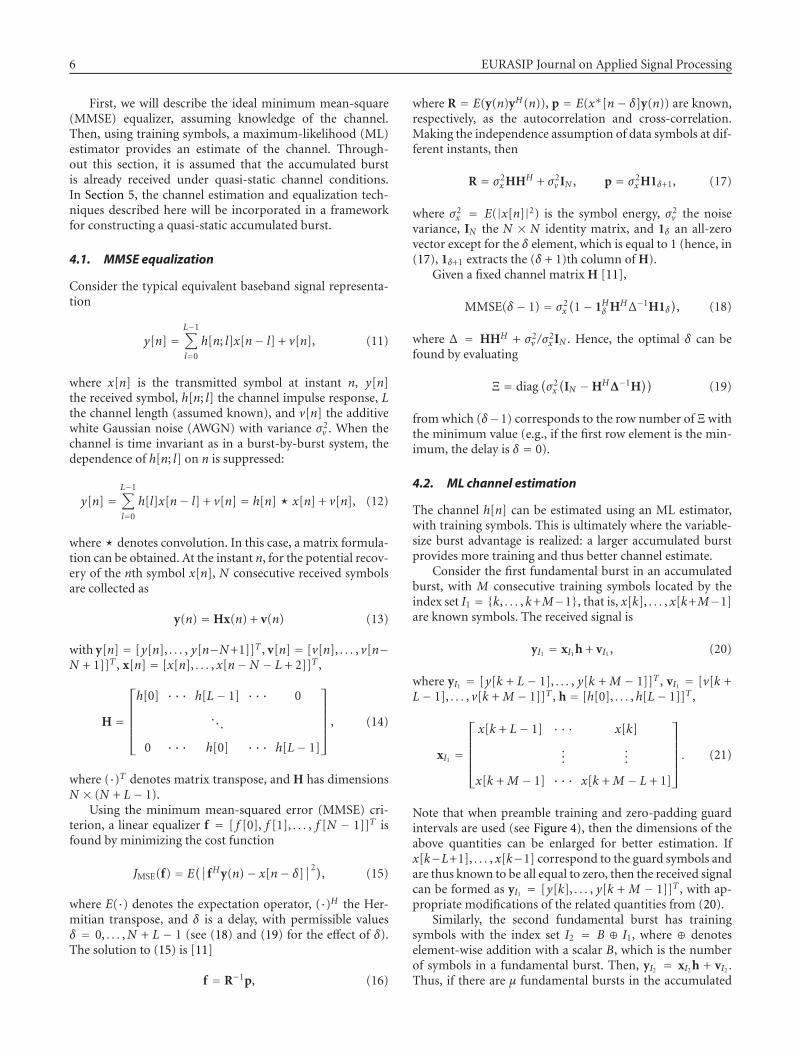
ρth: threshold for decision.Ntotal : total number of fundamental bursts to be processed.bsizemax: max. number of fundamental bursts in theaccumulated burst.s: fundamental burst defining start of the currentaccumulated burst.

(I) Initialization(1) Set s = 1

(II) Iterationfor i = 2, 3, . . . ,Ntotal

if (i− s + 1 ≥ bsizemax) or (i = Ntotal),(1) Set current accumulated burst =

all fundamental bursts from s to i,(2) Equalize the current accumulated burst,(3) Reset s = i + 1,

else if (ρed > ρth),(1) Set current accumulated burst =

all fundamental bursts from s to i− 1,(2) Equalize the current accumulated burst(3) Reset s = i,

endend

Algorithm 1: Variable-size burst receiver with channel tracking.

improvement compared to a fixed-size burst in time-varyingenvironments, the effect of threshold optimization will notbe explored. Instead, in Section 7, a sensibly predeterminedthreshold function ρth, weighted against the noise varianceσ2v , will be used to assess potential improvement.

5.3. Receiver processingwith a variable-size burst

Implicit in the tracking procedure is the requirement of abuffer for computing the intermediate h1 and h2, which in-troduces additional complexity and also latency. To allevi-ate the incurred penalties, a maximum burst size can be im-posed. Fortunately, as evidenced in Section 7, a modest burstsize can yield significant performance gain. In fact, when thereceiver already has sufficient training to equalize the chan-nel accurately, that is, approaching the MMSE lower-bound,enlarging the accumulated burst does not produce furtherappreciable improvement. Also, constraining the burst sizeminimizes the propagation of estimation errors. At low SNR,with inaccurate channel estimates, tracking can erroneouslyaccumulate more fundamental bursts than possible, thus vi-olating the quasi-static requirement.

Accounting for the above factors, Algorithm 1 shows aconceptual receiver procedure for processing variable-sizebursts. Essentially, while the accumulated burst has not ex-ceeded the maximum size, the receiver iteratively considersconsecutive candidate fundamental bursts for inclusion, us-ing a threshold-based change detection scheme.

5.4. Constrained optimization interpretation

Let the objective F(μ) = Mμ be the total number of trainingsymbols as a function ofM, the number of training symbols

in a fundamental burst (see (20)), and μ, the number of fun-damental bursts in the accumulated burst (see (22)). Notethat M is typically a fixed constant, defined by the trainingdensity. Also, let hi be the channel associated with the ith fun-damental burst in the accumulated burst. Then variable-sizeburst construction is equivalent to a mixed-integer optimiza-tion problem: [12].

Lemma 1. There exists a unique solution to the following burstconstruction problem:

maximize F(μ) =Mμ

subject to μ ∈ Z(an integer); μ ≤ bsizemax,

h1 = h2 = · · · = hμ (channel invariance).

(31)

Proof. The result follows trivially by noting that F(μ) isa strict monotonic increasing function of μ. Hence, con-strained to a bounded domain, there exists a unique maxi-mum.

Remarks

If, instead, the objective function is the training density,where the number of training symbols can be adapted perburst, then the optimization problem is not necessarilymixed integer (and M represents essentially a step-size pa-rameter). However, in this case the transceiver design wouldbe more complicated, with some form of feedback required.

Since the existence of a unique solution is guaranteed byLemma 1, an iterative search for the solution can be imple-mented. Here, the main difficulty is ensuring that the chan-nel invariance constraint in (31) is maintained. The channelshi are not known, and estimates hi must be used. Then inthe presence of noise and estimation error, with probabil-ity one, h1 = h2 = · · · = hμ, for all μ. Hence, consider in-stead the equivalent form of the constraint |hi+1 − hi|2 = 0,i = 1, . . . ,μ− 1 yielding the squared norm relaxation [12]

∣∣hi+1 − hi∣∣2 < ρth, i = 1, . . . ,μ− 1, (32)

where ρth is a small constant, allowing for some flexibilityin accommodating channel estimation error. Essentially, thisentails choosing ρth as in Section 5.2.

Also, at the kth iteration, instead of simply checking |hk−�hk−1|2 against the threshold, |hC − hP|2 as defined by (25) isused to guarantee the constraint. This allows for improvedestimation consistency since more training symbols are usedfor estimation with more iterations.

Algorithm 1 implements the described strategy to itera-tively search for μ, which approaches the optimal solution inthe squared norm sense.

6. ADAPTIVEMODULATION

The basic scheme of closed-loop burst-by-burst adaptivemodulation can be summarized as follows [3, 13].


(1) At the receiver, perform a channel-quality measure-ment, returning a channel metric.

(2) Relate this channel metric to a suitable modulationmode, which yields the highest throughput whilemaintaining the required level of QoS.

(3) Signal the selected modulation mode to the transmit-ter to be used in the next transmission burst.

Note that the average transmitted symbol energy σ2x canbe kept the same, regardless of the modulation mode in use.This alleviates the need of power control, which is typical foralternative systems operating in fading channels. The QoSis nonetheless guaranteed, by using the suitable modulationmode for an operating channel quality. In addition, the sym-bol rate is maintained constant so that the required band-width is unchanged, regardless of the selected modulationmode.

6.1. Channel metric

The most accurate metric for quantifying the channel qual-ity is the BER. However, since the BER is often difficult toestimate directly, alternatives are often used instead. For afrequency-non selective or flat-fading channel, the short-term signal-to-noise ratio (SNR) is an appropriate metric[3, 13]. For a frequency-selective channel, the short-termSNR is inadequate, since the influence of ISI must be takeninto account. Moreover the BER performance for frequency-selective channel is a complicated function of many factors,including channel length, power-delay profile, and even theform of equalizer used, for example, the number-taps in alinear equalizer, and the value of the equalizer delay. In thefollowing, we outline three possible approaches for comput-ing a channel metric, which can be used to guarantee a targetQoS by selecting the appropriate modulation mode.

(1) Exact residual ISI

Given enough side information, the exact probability of er-ror can be computed. Consider the overall equalized channelimpulse response:

g[n] = f ∗[n]� h[n], (33)

where f [n] and h[n] are the impulse responses of the equal-izer and the channel, respectively. Following [14], considerthe equalizer output at instant n

z[n] = f ∗[n]� y[n]

= g[δ]x[n− δ] +∑

k =δg[k]x[n− k] +

N−1∑

k=0f ∗[k]v[n− k],

(34)

where the first term is the desired signal component, thesecond term the residual ISI, and the last term the equal-ized noise. Note that g[n] is effectively an FIR filter of lengthN+L−1. Hence, for a particular input sequence xJ ofN+L−1

symbols, the corresponding residual ISI term is

DJ =∑

k =δg[k]xJ[n− k]. (35)

When usingM-PAM, the resulting probability of error is [14]

PM(DJ) = 2(M − 1)

MQ

⎛⎜⎝

√√√√(g[δ]−DJ

)2

σ2n

⎞⎟⎠ , (36)

where σ2n is the variance of the equalized noise

σ2n = σ2v

N−1∑

n=0

∣∣ f [n]∣∣2. (37)

Hence, for a particular channel, input sequence and M, theexact probability of error can be found. A channel metric canthen be defined as

ΓISI = DJ , (38)

and the appropriate modulation mode, that is, the value ofM, can be determined from (35) for a desired QoS. Unfortu-nately, this exact metric is not practical, since knowledge ofN +L− 1 data symbols surrounding the desired symbol x[δ]is required (which implies knowledge of the entire sequenceof data).

Alternatively, an average and an upper-bound probabilityof error can be found, respectively, as [14]

PM =∑

xJ

PM(DJ)P(xJ), (39)

PM(D∗J), D∗J = (M − 1)

∑

k =δ

∣∣g[k]∣∣, (40)

where (39) is an average over all possible xJ , and (40) is dueto the worst-case residual ISI. Unfortunately, the former iscomputationally expensive, while the latter tends to be ratherloose. In addition, for a fading environment, averaging overall fading-channel realizations is required. Thus the exactresidual ISI metric is only appropriate for channels with veryshort length.

(2) Pseudo-SNR

The pseudo-SNR is basically the SNR at the equalizer output:

pseudo-SNR = wanted signal powerresidual ISI + noise power

, (41)

and is defined in terms of the coefficients of a decision-feedback equalizer in [3]. Using a linear MMSE equalizerwith delay δ,

ΓpSNR = σ2x∣∣g[δ]

∣∣2

σ2x∑

k=δ∣∣g[k]

∣∣2 + σ2n(42)

for a particular channel realization, where σ2n is found using


(37). Note that as in [3], a Gaussian approximation of theresidual ISI term is made, and independence of the residualISI and noise is assumed. Then the BER formula in an AWGNchannel can be used. For example, the BER for a particularchannel realization with 4-QAM:

P(ΓpSNR

) = P(awgn)4-QAM

(ΓpSNR

) = Q(√

ΓpSNR), (43)

and more importantly the BER over a mobile fading channelcan be found, for a specificm-QAMmode, as

P(mf)m-QAM(γ) =

∫∞

0P(awgn)m-QAM

(ΓpSNR

)p(ΓpSNR, γ

)dΓpSNR,

(44)

where γ is the average channel SNR:

γ = E(∣∣h[n]� x[n]

∣∣2)

E(∣∣v[n]

∣∣2) , (45)

P(awgn)m-QAM(·) the AWGN BER expressions for the m-QAM

mode (e.g., can be found in [3, 14]); and p(ΓpSNR, γ) the pdfof the pseudo-SNR ΓpSNR over all fading channel realizations,at a certain average channel SNR γ. In general, the closed-form pdf is not available, and the (discretized) pdf needsto be computed numerically, at each γ of interest [3]. WithΓpSNR as a channel metric, the appropriate m-QAM mode isselected from (44) for a target QoS.

(3) MSE-basedmetric

The pseudo-SNR metric requires knowledge of the channelh[n]. For methods that find the equalizer f directly withoutestimating h[n], a channel metric can be defined based on theMSE computed at the equalizer output [5]. In the sequel, therelationship between the MSE-based metric and the pseudo-SNR is established.

At the equalizer output (34),

z[n] = f ∗[n]� y[n] = x[n− δ] + e[n], (46)

where x[n− δ] is the desired component, and e[n] the over-all residual equalization error, which, combines residual ISI,equalized noise, and also scaling. Then, the MSE is the equal-ization error variance,

σ2e = E(∣∣e[n]

∣∣2) = E(∣∣x[n− δ]− z[n]

∣∣2), (47)

and can be estimated using training symbols [5]. A corre-sponding channel metric is

ΓMSE = σ2xσ2e

. (48)

Table 2: Threshold-based switching rules for adaptive modulation.

Switching criterion Modulation mode0 ≤ ΓC < t1 V1

t1 ≤ ΓC < t2 V2

......

tQ−1 ≤ ΓC <∞ VQ

Making the assumption of independence between datasymbols, residual ISI, and noise,

ΓpSNR = σ2x∣∣g[δ]

∣∣2

σ2e − σ2x∣∣g[δ]− 1

∣∣2 . (49)

Comparing (48) and (49), the twometrics are identical wheng[δ] = 1, which occurs when the ISI is completely suppressedby the equalizer (at high SNR).

In general, the relationship between the probability of er-ror and MSE is not expressible in a simple closed form. Butan upperbound can be obtained [15],

Pe(σ2e) ≤ exp

(− 1− σ2e /σ

2x

σ2e

). (50)

Then, the same approach as (44) applies, using the pdf ofΓMSE, which is close to the pdf ΓpSNR at high SNR.

6.2. Threshold-basedmode adaptation

Consider a general channel metric ΓC , for example, ΓC =ΓpSNR, which quantifies in some manner the operating chan-nel quality. A threshold-based scheme can be constructedas follows [3, 5]. Designate the choice of available mod-ulation modes by Vq, q = 1, . . . ,Q, where Q is the totalnumber of available modulation modes; V1 is the constella-tion with the least number of points (most robust); and VQ

the highest (most efficient). Then Table 2 shows the switch-ing rules, based on a set of thresholds (t1, . . . , tQ−1), wheret1 < t2 < · · · < tQ−1 are chosen to guarantee some requiredlevel of QoS [3].

6.3. Thresholds selection

For a set of thresholds (t1, . . . , tQ−1), the mean throughput(number of bits per symbol) [3, 16]

B(γ) = BV1

∫ t1

0p(ΓC , γ

)dΓC

+Q−1∑

q=2BVq

∫ tq

tq−1p(ΓC , γ

)dΓC

+ BVQ

∫∞

tQ−1p(ΓC , γ

)dΓC ,

(51)

where BVq is the throughput associated with the Vq mode


Ntotal : total number of fundamental bursts to be processed.s: starting fundamental burst of current accumulated burst.γC : a channel quality metric (e.g., ΓpSNR).

(I) Initialization

(1) Set s = 1,(2) Measure channel metric γC using sth fundamental

burst,(3) Request QAM-mode(γC) to transmitter for

the rest of current accumulated bursts.

(II) Iterationfor i = 2, 3, . . . ,Ntotal

Track channel starting from sth fundamental burst(using tracking strategy from Section 5,Algorithm 1)

...if (channel change detected at ith fundamental burst)

(1) Set current accumulated burst =all fundamental bursts from s to i− 1,

(2) Decode the current accumulated burst,(3) Reset s = i (i.e., start of new accumulated, burst)(4) Measure channel metric γC using sth

fundamental burst,(5) Request QAM-mode(γC) to Tx for

the rest of the new accumulated burst.end

end

Algorithm 2: Adaptive modulation with variable-size burst.

(e.g., throughput of 16-QAM is 4 bps). In a fading channel,the average BER for adaptive modulation

P(mf)AM (γ) = 1

B(γ)

[BV1

∫ t1

0P(awgn)V1

(ΓC)p(ΓC , γ

)dΓC

+Q−1∑

q=2BVq

∫ tq

tq−1P(awgn)Vq

(ΓC)p(ΓC , γ

)dΓC

+ BVQ

∫∞

tQ−1P(awgn)VQ

(ΓC)p(ΓC , γ

)dΓC

].

(52)

Hence, with (52), the thresholds can be optimized to producea desired QoS, for example, using a cost function based ondesired BER and average throughput [3, 16].

6.4. Integrationwith variable-size burst construction

A two-layer strategy is used for adaptation: variable-sizeburst construction in the first layer, and adaptive modula-tion method in the second. Feedback is required only in thesecond layer. A conceptual algorithm for this strategy is sum-marized in Algorithm 2.

Note that the channel quality is measured once per accu-mulated burst, that is, the metric obtained with the startingfundamental burst selects the modulation mode for the en-tire accumulated burst. This is valid because, with channeltracking, the same channel condition, that is, same channelquality, applies to the entire burst.

6.5. Proof of optimality

Let the objective G(q) = log2 q be the throughput (num-ber of transmitted bits per symbol) as a function of themodulation mode q. For simplicity, let us assume that thereare four modulation modes, that is, q = 0 (no transmis-sion), 2 (BPSK), 4 (4-QAM), 16 (16-QAM). Then adaptivemodulation with variable-size burst is equivalent to

maximize G(q) = log2 q,

subject to μ ∈ Z(an integer), μ ≤ bsizemax,

h1 = h2 = · · · = hμ (channel invariance),

BER(μ, q),≤ BERmax, q ∈ {0, 2, 4, 16},σ2x = constant,

(53)

where BERmax specifies the maximum acceptable bit-errorrate for a desired QoS, and σ2x = E(|x[n]|2) is the symbolenergy.

Proposition 1. Under the constraints in (53), the given jointoptimization problem of burst construction and adaptive mod-ulation has a unique solution. Moreover, the joint optimizationis actually separable, that is, burst construction and adaptivemodulation can be performed separately in a two-layer strat-egy.

Proof. (i) The objective G(q) is a strict monotonic increasingfunction of q.

(ii) When channel estimation is performed using train-ing symbols, BER is also a function of μ. Under the firstthree constraints, essentially those from (31), the accumu-lated burst constructed has more training symbols and alsosatisfies quasi-static channel requirements. Then, BER is astrict monotonic decreasing function of μ.

(iii) Under the last constraint of constant symbol energy,BER is a strict monotonic increasing function of q since in-creasing q decreases the minimum distance between constel-lation points.

(iv) From (i), (ii), and (iii), a unique solution exists on abounded domain.

(v) Moreover, to optimally satisfy the fourth BER con-straint, μ needs to be as large as possible (for any q). Thismeans that optimization of burst size (which depends on theunderlying channel, not on the modulation-mode) can beperformed first, followed by the modulation mode search(recall that burst construction deals with channel rate ofchange, while adaptive modulation addresses the channelquality).

(vi) In other words, a two-layer strategy can be utilized.Once the optimal μ is found as the solution of (31), the


optimal q can then be searched from the given mode choices,producing the largest q that satisfies the BER constraint.

Remarks

The channel invariance constraint is crucial. Otherwise, if thechannel changes between bursts, then increasing the num-ber of training symbols or the modulation mode may ormay not improve estimation, depending on the operatingchannel SNR. In other words, without this constraint, themonotonicity of BER(μ, q) may no longer hold. As such,nonunique local maxima may exist on the BER surface overthe bounded domain, and the problem would no longer beseparable.

Proposition 2. For each modulation mode q, there is a bi-jection (one-to-one and onto mapping) between the (pseudo-SNR) channel metric and the BER.

Proof. This should be quite obvious by construction of anychannel metric, because otherwise the constructed metric isnot a good metric at all. For the specific case of ΓpSNR, thepseudo-SNR metric, the key is to realize that both ΓpSNR andBER are continuous and strict monotonic decreasing func-tions of the average channel SNR γ, evident from (42), (44),and (45).

In other words, there exist φ,ψ : BER = φ(γ),ΓpSNR =ψ(γ), where φ,ψ are both bijective (for φ, see (44)). Beingbijections, φ,ψ have bijective inverses: γ = φ−1(BER), γ =ψ−1(ΓpSNR). Then, ΓpSNR = ψ(φ−1(BER)).

Theoretically, Proposition 2 implies that, when using thechannel metric ΓpSNR to maintain the BER constraint in (53),the equivalent condition is ΓpSNR(μ, q) ≤ tq(BERmax), wheretq(·) = ψ(φ−1(·)), for each q. However, note that the above isa purely existential construction, since it is usually difficult tocompute the inverses in closed form, for example, comput-ing γ from BER using (44). Therefore, in practice, the opti-mal thresholds are usually determined empirically for adap-tive modulation [3, 16], as discussed in Section 6.3.

With the above considerations, Algorithm 2 implementsa two-layer strategy that iteratively searches for the opti-mal (μ, q). The switching thresholds (with guaranteed op-timal existence by Proposition 2) are empirically approxi-mated and used according to Table 2 for adaptive modula-tion.

Remarks

Due to the particular forms of the objective and constraintsconsidered here, the optimization can be decoupled as twoseparate layers. However, this is not always possible. Chang-ing the objective function, for example, addition of delaycost, may necessitate cross-layer optimization. In addition,with more extensive solution spaces (larger bsizemax andmore mode choices), an exhaustive search quickly becomesprohibitively complex due to the combinatorial nature of the

mixed-integer problem. For all these cases, suboptimal tech-niques, such as convexification and relaxation [12], may beapplied to reduce complexity.

6.6. Metric errors

It is important to realize that optimality of the above tech-niques is only guaranteed under ideal situations. In practice,estimation errors lead to constraint violations and thereforesuboptimal solutions. In particular, with respect to adaptivemodulation, not only can metric errors occur due to insuffi-cient training, delays in transceiver feedback also mean thattransmitter mode switching may be too slow.

Algorithm 2 implements closed-loop metric signalling[3], and thus has a minimum latency of one fundamentalburst. In other words, even without feedback delay, the met-ric estimated using the current burst is not used to update themodulation mode until the next transmitted burst, duringwhich time, depending on the Doppler frequency, the chan-nel quality may have changed significantly. In real applica-tions, with feedback delay, the actual latency is even higher.Especially when the channel is changing rapidly, this latencycan cause incorrect modes to be invoked by the transmitterreceiving outdated metrics.

Under certain conditions, it may be possible to predictthe upcomingmetrics, thusmitigating the latency effect. Var-ious important considerations in practical implementationsof adaptive modulation are surveyed in [3]. In Section 7.5,the effect of latency in the metric estimation will be evalu-ated by simulation.

7. SIMULATION EXAMPLES

Simulation parameters used are: carrier frequency fc =3GHz, symbol duration TS = 2 μs, fundamental burst size= 80 symbols, training density = 10% (i.e., 8 symbols perfundamental burst), normalized data symbols with σ2x = 1,4-QAM for fixed-modulation simulations, number of equal-izer taps N = 50. The power-delay profile is exponential(same shape as Table 1), with delay positions [0, 4, 6, 7]×TS,so that the channel length L = 8.

The maximum accumulated burst size bsizemax equals 4fundamental bursts. The threshold function ρth is definedpiece-wise over the SNR-range η ∈ [0, 40] dB:

ρth(η) =

⎧⎪⎪⎪⎪⎪⎨⎪⎪⎪⎪⎪⎩

4σ2v , η ≤ 20,

2σ2v , 20 < η ≤ 30,

σ2v , 30 < η ≤ 40,

(54)

where σ2v is the channel noise variance. This threshold func-tion fulfills the criterion for avoiding potential error floors athigh SNR as discussed in Section 5.2: allows larger channelestimation error at low SNR, while forcing smaller estima-tion error at high SNR.


100

10−1

10−2

10−3

10−4

10−5

10−6

BER

0 5 10 15 20 25 30 35 40

Average channel SNR

MMSEVariable-size burstFixed small burst

Fixed big burstQuasi-static burst

Figure 5: BER performance over fading channel with fmTs = 1 ×10−4 or mobile speed vm = 18 km/h.

7.1. Variable-size burst in a slow-fading channel

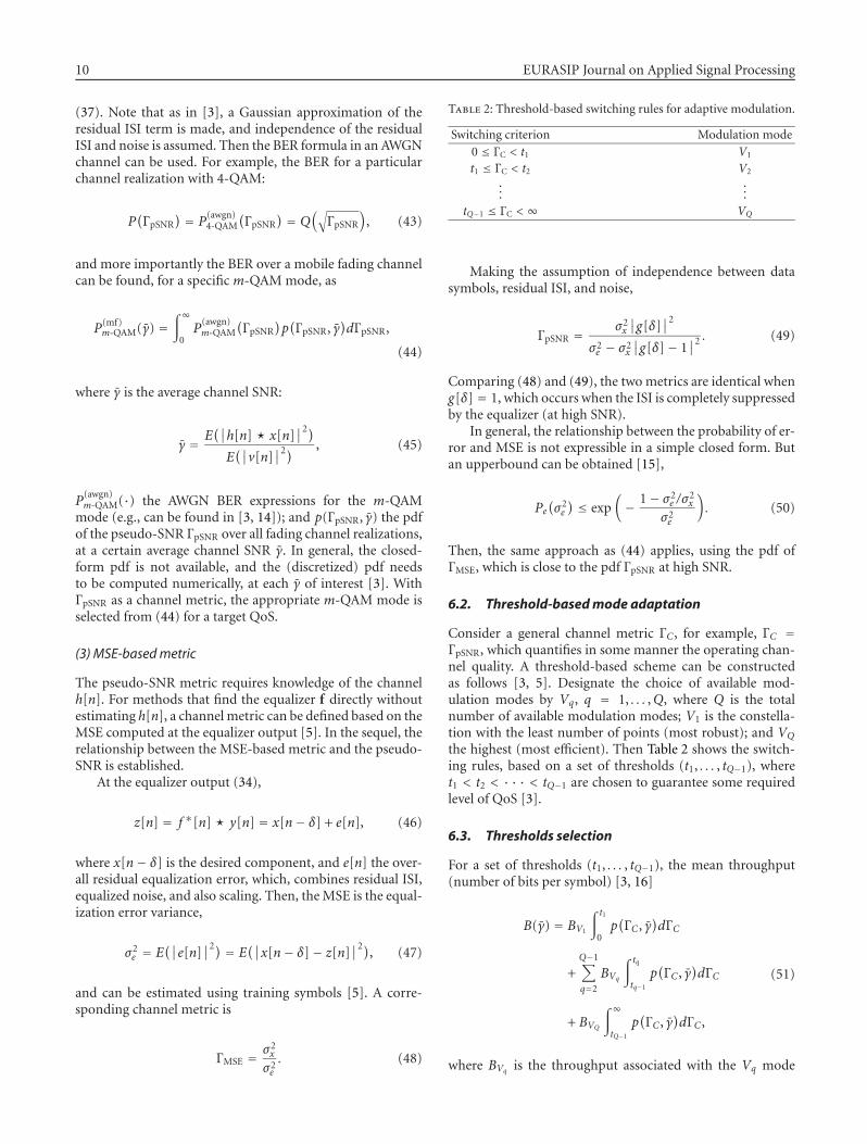
Here, the channel is characterized by one Doppler state, withfmTs = 1 × 10−4 or mobile speed vm = 18 km/h. Figure5 shows the resulting BER performances for the followingschemes.

(1) MMSE

Obtained using a fixed-size burst equal to the fundamentalburst, and with a priori knowledge of the channel. This is thelower-bound for other cases.

(2) Quasi-static burst

Also obtained using a fixed-size fundamental burst, but withan estimated channel. There is insufficient training for accu-rate estimation, manifested by a large performance gap fromthe lower bound.

(3) Fixed small burst

Obtained using a fixed-size burst equal to two fundamentalbursts. More training symbols are available compared to thequasi-static burst, resulting in performance improvement.

(4) Fixed big burst

Obtained using a fixed-size burst equal to four fundamentalbursts. This scheme approaches the MMSE performance atlow SNR, but suffers from an error floor at high SNR dueto quasi-static violation being a bottleneck in the absence ofnoise.

100

10−1

10−2

10−3

10−4

10−5

10−6

BER

0 5 10 15 20 25 30 35 40

Average channel SNR



Figure 6: BER performance over fading channel with fmTs = 9 ×10−4 or mobile speed vm = 162 km/h.

(5) Variable-size burst

Inherits the best characteristics of the previous two fixed-sizeburst schemes, with good performance at low SNR and noerror floor at high SNR.

7.2. Variable-size burst in a fast-fading channel

Here, fmTs = 9 × 10−4, corresponding to vm = 162 km/h.Figure 6 shows the resulting performances. Due to construc-tion, the MMSE and quasi-static burst have identical perfor-mances as before. In this more rapidly varying scenario, bothfixed-size burst schemes suffer from error floors. By contrast,the variable-size burst is able to compensate for the fasterchannel changes, without being affected by an error floor dueto quasi-static violations. Although not as significant as in aslow fading scenario, the variable-size burst still delivers bet-ter performance compared to a quasi-static burst.

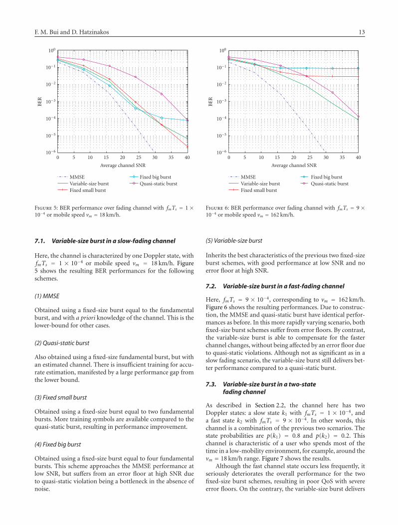
7.3. Variable-size burst in a two-statefading channel

As described in Section 2.2, the channel here has twoDoppler states: a slow state k1 with fmTs = 1 × 10−4, anda fast state k2 with fmTs = 9 × 10−4. In other words, thischannel is a combination of the previous two scenarios. Thestate probabilities are p(k1) = 0.8 and p(k2) = 0.2. Thischannel is characteristic of a user who spends most of thetime in a low-mobility environment, for example, around thevm = 18 km/h range. Figure 7 shows the results.

Although the fast channel state occurs less frequently, itseriously deteriorates the overall performance for the twofixed-size burst schemes, resulting in poor QoS with severeerror floors. On the contrary, the variable-size burst delivers


100

10−1

10−2

10−3

10−4

10−5

10−6

BER

0 5 10 15 20 25 30 35 40

Average channel SNR



Figure 7: BER performance over fading channel with 2 Dopplerstates: k1 with fmTs = 1 × 10−4 and k2 with fmTs = 9 × 10−4; thestate probabilities are p(k1) = 0.8 and p(k2) = 0.2.

performance gain by exploiting the slower channel state,without being affected by an error floor due to the fast state.

7.4. Average burst length of the variable-size burst

Figure 8 shows the average burst length in the previous chan-nel settings. In a slow fading channel, the burst is closer tothe maximum admissible length (bsizemax = 4). But in a fastfading channel, the burst length tends to be shorter in orderto satisfy the quasi-static assumption. In a two-state channel,the average burst length is somewhere in between, regulatedessentially by the threshold function ρth.

7.5. Adaptivemodulation: BER performance

The previous simulations show that the two fixed-size burstschemes severely fail in a two-state channel, even with fixedmodulation. Hence, we will focus on the MMSE, quasi-staticand variable-size bursts for adaptive modulation.

The pseudo-SNR metric ΓpSNR is used with thresholdsand associated modulation modes summarized in Table 3.

Transmission blocking (no transmission) is invoked forvery poor conditions. The highest-throughput mode is 16-QAM, transmitting 4 bits/symbol. To illustrate the effect ofmetric errors as discussed in Section 6.6, two cases are con-sidered: (i) no feedback delay, resulting in (minimum) la-tency of 1 burst; (ii) feedback delay of 2 bursts, causing over-all latency of 3 bursts. Figure 9 shows the resulting BER per-formances.

Without feedback delay, the MMSE scheme is able tolimit the maximum BER to 10−4, for the SNR range greaterthan 15 dB. By modifying the thresholds, this range can bechanged accordingly, but at the loss of throughput efficiency

3.5

3

2.5

2

1.5

1

Numberof

fundamentalbursts

0 5 10 15 20 25 30 35 40

Average channel SNR

fmTs = 1× 10−4

fmTs = 9× 10−4

Two Doppler states

Figure 8: Average burst length (in terms of number of fundamentalbursts) of a variable-size burst.

Table 3: Switching thresholds for adaptive modulation.

Channel metric (dB) Modulation mode0 ≤ ΓpSNR < 8 No transmission

8 ≤ ΓpSNR < 12 BPSK

12 ≤ ΓpSNR < 20 4-QAM

20 ≤ ΓpSNR <∞ 16-QAM

(Figure 10). The obtained results reveal variable-size burst assuperior to the fixed-size scheme, guaranteeing a better QoSquantified by the BER.

With delay, the overall QoS is lowered for all cases. Thisreduction is more noticeable at low SNR since an erroneousmetric here implies incorrect invocation of a higher-ordermode. By contrast, at high SNR where a higher-order mod-ulation mode is usually already appropriate, an incorrectinvocation causes less degradation. And as mentioned inSection 6.6, in certain cases, it may be possible to performmetric prediction to mitigate latency [3].

7.6. Adaptivemodulation: throughput performance

A complete comparison of various burst schemes, when us-ing adaptive modulation, also requires examining the corre-sponding throughputs (number of bits per symbol), depictedin Figure 10.

For throughput, as found in [3], the effect of latencyis less significant, with only small performance differencefrom the ideal case. At low SNR, the MMSE has the lowestthroughput. In fact, transmission blocking needs to be thedominant mode here to maintain QoS. Fewer instances of


10−1

10−2

10−3

10−4

10−5

BER

0 5 10 15 20 25 30 35 40

Average channel SNR

MMSEMMSE (delayed)Variable size

Variable size (delayed)Quasi-staticQuasi-static (delayed)

Figure 9: Adaptivemodulation BER performance over fading chan-nel with 2 Doppler states: k1 with fmTs = 1 × 10−4 and k2 withfmTs = 9 × 10−4; the state probabilities are p(k1) = 0.8 andp(k2) = 0.2.

4

3.5

3

2.5

2

1.5

1

0.5

0

Through

put(bps)

0 5 10 15 20 25 30 35 40

Average channel SNR

MMSEMMSE (delayed)Variable size

Variable size (delayed)Quasi-staticQuasi-static (delayed)

Figure 10: Adaptive modulation throughput performance corre-sponding to Figure 9.

transmission blocking are observed for the variable-size andquasi-static bursts. The reason is that, at low SNR, an accu-rate channel metric is not available for optimal modulationmode selection. At high SNR, all schemes have nearly iden-tical throughputs, since the estimation of channel metric ismore accurate without noise.

The combined BER and throughput performances dem-onstrate the superiority of a variable-size burst compared

to its fixed-size counterpart. It maintains almost identicalthroughput, but supports much improved QoS.

8. CONCLUDING REMARKS

In this work, two approaches for efficient and reliable com-munications in time-varying mobile environments are pre-sented: variable-size burst construction and adaptive mod-ulation. It has been shown that, when the underlying time-varying channel is dominated by a slower state, reliable andefficient communication is still possible using a conventionalburst-by-burst receiver methodology.

If the channel is dominated by a fast channel state, thevariable-size burst performance approaches that of the quasi-static burst, with poor QoS and efficiency. For these sce-narios, as mentioned in Section 1, the variable-size burstmethodology can be combined with basis-expansion chan-nel models to deliver improved performance at the cost ofcomplexity [6].

ACKNOWLEDGMENTS

The authors thank the anonymous referees whose insight-ful reviews were instrumental in improving the paper. Weare also grateful to the Editor Professor Geert Leus for sug-gesting important modifications. This work was supportedby the Natural Sciences and Engineering Research Council ofCanada. Some of the material in this paper was presented atIEEE Globecom 2004, Dallas, Tex.

REFERENCES

[1] T. S. Rappaport,Wireless Communications: Principles and Prac-tice, Prentice Hall, Englewood Cliffs, NJ, USA, 1996.

[2] R. Steele and L. Hanzo,Mobile Radio Communications: Secondand Third Generation Cellular and WATM Systems, JohnWiley& Sons, New York, NY, USA, 1999.

[3] L. Hanzo, C.Wong, andM. Yee, Adaptive Wireless Transceivers:Turbo- Coded, Turbo-Equalized and Space-Time Coded TDMA,CDMA, and OFDM Systems, John Wiley & Sons, New York,NY, USA, 2002.

[4] F. M. Bui and D. Hatzinakos, “A receiver-based variable-size-burst equalization strategy for spectrally efficient wire-less communications,” IEEE Transactions on Signal Processing,vol. 53, no. 11, pp. 4304–4314, 2005.

[5] F. M. Bui and D. Hatzinakos, “Adaptive modulation usingvariable-size burst for spectrally efficient interference sup-pression in wireless communications,” in Proceedings of IEEEGlobal Telecommunications Conference (GLOBECOM ’04),vol. 2, pp. 898–902, Dallas, Tex, USA, November-December2004.

[6] F. M. Bui and D. Hatzinakos, “Identification and tracking ofrapidly time-varying mobile channels for improved equaliza-tion: a basis-expansion model approach,” to appear in The 5thInternational Symposium on Communication Systems, Networkand Digital Signal Processing (CSNDSP ’06), Patras, Greece.

[7] G. B. Giannakis and C. Tepedelenlioglu, “Basis expansionmodels and diversity techniques for blind identification andequalization of time-varying channels,” Proceedings of theIEEE, vol. 86, no. 10, pp. 1969–1986, 1998.


[8] I. Barhumi, G. Leus, and M. Moonen, “Time-varying FIRequalization for doubly selective channels,” IEEE Transactionson Wireless Communications, vol. 4, no. 1, pp. 202–214, 2005.

[9] M. Patzold,Mobile Fading Channels, John Wiley & Sons, NewYork, NY, USA, 1st edition, 2002.

[10] M. Dong and L. Tong, “Optimal design and placement of pilotsymbols for channel estimation,” IEEE Transactions on SignalProcessing, vol. 50, no. 12, pp. 3055–3069, 2002.

[11] S. Haykin, Adaptive Filter Theory, Prentice Hall, EnglewoodCliffs, NJ, USA, 3rd edition, 1996.

[12] C. A. Floudas, Nonlinear and Mixed-Integer Optimization:Fundamentals and Applications, Oxford University Press, NewYork, NY, USA, 1995.

[13] S. Catreux, V. Erceg, D. Gesbert, and R. W. Heath, “Adaptivemodulation and MIMO coding for broadband wireless datanetworks,” IEEE Communications Magazine, vol. 40, no. 6, pp.108–115, 2002.

[14] J. G. Proakis, Digital Communications, McGraw Hill, NewYork, NY, USA, 4th edition, 2001.

[15] P. Balaban and J. Salz, “Optimum diversity combining andequalization in digital data transmission with applicationsto cellular mobile radio. I: theoretical considerations,” IEEETransactions on Communications, vol. 40, no. 5, pp. 885–894,1992.

[16] C. H. Wong and L. Hanzo, “Upper-bound performance of awide-band adaptive modem,” IEEE Transactions on Commu-nications, vol. 48, no. 3, pp. 367–369, 2000.

Francis Minhthang Bui received the B.A.degree in French language and the B.S. de-gree in electrical engineering from the Uni-versity of Calgary, Alberta, Canada, in 2001.He then completed the M.A.S. degree inelectrical engineering in 2003 from the Uni-versity of Toronto, Ontario, Canada, wherehe is currently pursuing the Ph.D. degree.His research interests include resource al-location and signal processing methods forpower- and spectrum-efficient communications.

Dimitrios Hatzinakos received the Diplo-ma degree from the University of Thessa-loniki, Greece, in 1983, the M.A.S. degreefrom the University of Ottawa, Canada, in1986, and the Ph.D. degree from North-eastern University, Boston, Mass, in 1990,all in electrical engineering. In September1990, he joined the Department of Electri-cal and Computer Engineering, Universityof Toronto, where now he holds the rank ofProfessor with tenure. Also, he served as Chair of the Communica-tions Group of the department during the period July 1999 to June2004. Since November 2004, he is the holder of the Bell CanadaChair in Multimedia at the University of Toronto. His research in-terests are in the areas of multimedia signal processsing and com-munications. He is the author/coauthor of more than 150 papersin technical journals and conference proceedings, and he has con-tributed to 8 books in his areas of interest.

spectrallyefﬁcientcommunicationovertime-varying … · quality of service ... while maintaining...

Documents