spectrum occupancy measurements and evaluation · 2012-11-06 · rep. itu-r sm.2256 1 report itu-r...
TRANSCRIPT
Report ITU-R SM.2256(09/2012)
Spectrum occupancy measurements and evaluation
SM Series
Spectrum management

ii Rep. ITU-R SM.2256
Foreword
The role of the Radiocommunication Sector is to ensure the rational, equitable, efficient and economical use of the radio-frequency spectrum by all radiocommunication services, including satellite services, and carry out studies without limit of frequency range on the basis of which Recommendations are adopted.
The regulatory and policy functions of the Radiocommunication Sector are performed by World and Regional Radiocommunication Conferences and Radiocommunication Assemblies supported by Study Groups.
Policy on Intellectual Property Right (IPR)
ITU-R policy on IPR is described in the Common Patent Policy for ITU-T/ITU-R/ISO/IEC referenced in Annex 1 of Resolution ITU-R 1. Forms to be used for the submission of patent statements and licensing declarations by patent holders are available from http://www.itu.int/ITU-R/go/patents/en where the Guidelines for Implementation of the Common Patent Policy for ITU-T/ITU-R/ISO/IEC and the ITU-R patent information database can also be found.
Series of ITU-R Reports
(Also available online at http://www.itu.int/publ/R-REP/en)
Series Title
BO Satellite delivery
BR Recording for production, archival and play-out; film for television
BS Broadcasting service (sound)
BT Broadcasting service (television)
F Fixed service
M Mobile, radiodetermination, amateur and related satellite services
P Radiowave propagation
RA Radio astronomy
RS Remote sensing systems
S Fixed-satellite service
SA Space applications and meteorology
SF Frequency sharing and coordination between fixed-satellite and fixed service systems
SM Spectrum management
Note: This ITU-R Report was approved in English by the Study Group under the procedure detailed in Resolution ITU-R 1.
Electronic Publication Geneva, 2012
ITU 2012
All rights reserved. No part of this publication may be reproduced, by any means whatsoever, without written permission of ITU.

Rep. ITU-R SM.2256 1
REPORT ITU-R SM.2256
Spectrum occupancy measurements and evaluation
(2012)
Summary
Spectrum occupancy measurements and evaluation in modern RF environments with increasing density of digital systems and frequency bands shared by different radio services become a more and more complex and challenging task for Monitoring Services. Based on Recommendations ITU-R SM.1880, ITU-R SM.1809, and information provided in the 2011 Edition of the ITU Handbook on Spectrum Monitoring, this draft new Report provides a far more detailed discussion on different approaches to spectrum occupancy measurements, possible issues related to them and their solutions.
TABLE OF CONTENTS
Page
1 Introduction .................................................................................................................... 4
2 Terms and definitions ..................................................................................................... 5
2.1 Spectrum resource .............................................................................................. 5
2.2 Frequency channel occupancy measurement ...................................................... 5
2.3 Frequency band occupancy measurement .......................................................... 5
2.4 Measurement area ............................................................................................... 5
2.5 Duration of monitoring (TT) ................................................................................ 6
2.6 Sample measurement time (TM) .......................................................................... 6
2.7 Observation time (TObs) ...................................................................................... 6
2.8 Revisit time (TR) ................................................................................................. 6
2.9 Occupancy time (TO) .......................................................................................... 6
2.10 Integration time (TI) ............................................................................................ 7
2.11 Maximum number of channels (NCh) .................................................................. 7
2.12 Transmission length ............................................................................................ 7
2.13 Threshold ............................................................................................................ 7
2.14 Busy hour ............................................................................................................ 7
2.15 Access delay ....................................................................................................... 7
2.16 Frequency channel occupancy (FCO) ................................................................ 7
2.17 Frequency band occupancy (FBO) ..................................................................... 8
2.18 Spectrum resource occupancy (SRO) ................................................................. 8

2 Rep. ITU-R SM.2256
Page
3 Measurement parameters ................................................................................................ 10
3.1 Selectivity ........................................................................................................... 10
3.2 Signal to noise ratio ............................................................................................ 11
3.3 Dynamic range .................................................................................................... 12
3.4 Threshold ............................................................................................................ 12
3.4.1 Pre-set threshold ................................................................................... 12
3.4.2 Dynamic threshold ............................................................................... 13
3.5 Measurement timing ........................................................................................... 15
3.6 Directivity of the measurement antenna ............................................................. 17
4 Site considerations .......................................................................................................... 18
5 Measurement procedure ................................................................................................. 20
5.1 FCO measurement with a scanning receiver ...................................................... 20
5.2 FBO with a sweeping analyser ........................................................................... 20
5.3 FBO with FFT methods ...................................................................................... 20
6 Calculation of occupancy ............................................................................................... 21
6.1 Combining measurement samples on neighbouring frequencies ....................... 21
6.2 Classifying emissions in bands with different channel widths ........................... 22
7 Presentation of results ..................................................................................................... 23
7.1 Traffic on a single channel ................................................................................. 23
7.2 Occupancy on multiple channels ........................................................................ 24
7.3 Frequency band occupancy ................................................................................. 26
7.4 Spectrum resource occupancy ............................................................................ 28
7.5 Availability of results ......................................................................................... 29
8 Special occupancy measurements .................................................................................. 29
8.1 Frequency channel occupancy in frequency bands allocated to point-to-point systems of fixed service ...................................................................................... 29
8.2 Separation of occupancy for different users in a shared frequency resource ..... 30
8.3 Spectrum occupancy measurement of WLAN (Wireless Local Area Networks) in 2.4 GHz ISM band ........................................................................ 31
8.4 Determining the necessary channels for the transition from analogue to digital trunked systems .................................................................................................. 32
8.5 Estimation of RF use by different radio services in shared bands ...................... 35

Rep. ITU-R SM.2256 3
Page
9 Uncertainty considerations ............................................................................................. 35
10 Interpretation and usage of results .................................................................................. 36
10.1 General ................................................................................................................ 36
10.2 Interpretation of occupancy results in shared channels ...................................... 36
10.3 Using occupancy data to assess spectrum utilization ......................................... 36
11 Conclusions .................................................................................................................... 37
Annex 1 – Probabilistic approach to spectrum occupancy measurements and relevant measurement data handling procedures .......................................................................... 38
A Preface ............................................................................................................................ 38
A1 General description of the approach ............................................................................... 38
A2 Concept of spectrum occupancy ..................................................................................... 39
A2.1 Spectrum occupancy as a statistical concept ...................................................... 39
A2.2 Occupancy measurement error ........................................................................... 40
A2.3 Accuracy and confidence level of occupancy measurement .............................. 41
A2.4 Parameters affecting the statistical confidence of occupancy measurement ...... 42
A2.4.1 Pulsed and lengthy signals and signal flow rate. ................................. 42
A2.4.2 Relative instability of revisit time ........................................................ 43
A2.4.3 Use of lock-in and lock-out measuring systems for occupancy measurements ....................................................................................... 43
A3 Measuring procedures..................................................................................................... 44
A3.1 Recommendations for measuring occupancy with lock-in measuring systems . 44
A3.1.1 Data collection ..................................................................................... 44
A3.1.2 Occupancy measurement rule .............................................................. 44
A3.1.3 Selecting the number of samples ......................................................... 44
A3.1.4 Effect of incorrect choice of number of samples on the confidence level of the occupancy measurement ................................................... 47
A3.2 Recommendations for measuring occupancy with lock-out measuring systems 48
A3.2.1 Data collection ..................................................................................... 48
A3.2.2 Occupancy calculation rule .................................................................. 49
A3.2.3 Selecting the number of samples ......................................................... 49

4 Rep. ITU-R SM.2256
Page
A4 Typical examples of the impact of signal flow rate in the radio channel on the confidence level of spectrum occupancy calculations .................................................... 49
A4.1 Case A: One single signal present in the integration time .................................. 49
A4.2 Case B: Twelve signals during the integration time ........................................... 50
A4.3 Case C: Several dozen signals within the integration time ................................. 50
Reference to Annex A .............................................................................................................. 51
1 Introduction
The increasing use of radio makes it more and more difficult to accommodate all users in the limited spectrum available. Some frequency bands are already overcrowded at times and spectrum managers more often need to know the actual occupancy in certain frequency bands.
The following ITU documentation concerning occupancy has been taken into account when developing this report:
• Question ITU-R 233/1
Raised in 2007, this question calls for studies on methods to measure, evaluate and present frequency channel and band occupancy measurements.
• Recommendation ITU-R SM.1880
This Recommendation describes different aspects to consider when performing occupancy measurements and shows ways to present the results.
• Recommendation ITU-R SM.1809
This Recommendation defines a common data format for channel occupancy measurement results enabling the exchange of this data between administrations using different hard- and software for the actual measurement.
• Handbook on Spectrum Monitoring, Chapter 4.11
The 2011 edition of this Handbook summarizes occupancy measurement methods described in more detail in the Recommendations above.
The following factors, however, make it more and more difficult to measure spectrum occupancy and present the results in a way that spectrum managers can easily derive the necessary information:
• Self-organizing radio systems
Some modern radio systems do not have a single and/or fixed frequency that they operate on. Instead, they can sense the current occupancy inside a certain frequency band and automatically select a frequency that is currently free. The next time this device accesses the spectrum, the selected frequency may be different. One example of this behaviour is the DECT personal phone system.
• Frequency agile radio systems
Some radio systems change frequency very fast based on a fixed or even flexible scheme that appears random to an occupancy measurement system. One example is Bluetooth. Standard occupancy measurement systems usually are not fast enough to capture each short burst and may regard the whole frequency band as being used although only one station is active.

Rep. ITU-R SM.2256 5
• Pulsed (bursted) digital systems
Digital systems using TDMA multiple access methods usually transmit in bursts. Even if an occupancy measurement system would be fast enough to capture every single burst, the question still arises how occupancy is defined in this case: Should the frequency be regarded as being occupied just because one time slot is used, or should it state the amount of time in between the bursts as “available”?
• Frequency bands shared by users with different bandwidths
In some frequency bands, co-existing systems may have a completely different channel bandwidth and spacing. One example is the UHF broadcast band which may be used by Television transmitters having 8 MHz channel bandwidth and wireless microphones having 25 kHz spacing. An occupancy measurement with an 8 MHz resolution may show the occupied TV channels but cannot recognize wireless microphones occupying only a fraction of a TV channel. If the measurement is done on the basis of a 25 kHz channel spacing, a TV transmission would show up as a series of adjacent fully occupied wireless microphone channels.
This report describes the different aspects of measuring and evaluating spectrum occupancy in a more detailed way, also addressing the aspects mentioned above.
2 Terms and definitions
2.1 Spectrum resource
Spectrum resource describes the availability of spectrum in terms of space (e.g. location, service area), time and number of channels (in a channelized band) that all users on a certain territory may access.
Regarding a single frequency assignment, the spectrum resource may be only one single frequency channel. In case of self-organizing networks such as trunked networks or cellular systems, the spectrum resource may consist of all frequency channels in a certain band but may be limited in time, e. g. one time slot in a TDMA system.
Hence, the spectrum resource very much depends on the radio service and the specific problem under consideration.
2.2 Frequency channel occupancy measurement
Measurement of individual channels, either with the same or with different channel width, and possibly spread over several different frequency bands to determine the degree (percentage) of occupancy of these channels.
2.3 Frequency band occupancy measurement
Measurement of a frequency band, specified by start and stop frequency, with a step width (or frequency resolution) that is usually smaller than the channel spacing, to determine the degree of occupancy over the whole band.
2.4 Measurement area
In this context, the measurement area is the area for which the occupancy results are valid. A frequency or channel determined to have certain occupancy can be assumed to be representative for any location inside the measurement area, not only at the location of the monitoring antenna.

6 Rep. ITU-R SM.2256
2.5 Duration of monitoring (TT)
This is the total time during which the occupancy measurements are carried out.
Common monitoring durations are 24 h, working hours or another appropriate period. The optimum duration of monitoring depends on the purpose of the occupancy measurement and the available a priori knowledge about the behaviour of the radio systems using the spectrum resource. If, for example, the band to be measured contains only broadcast stations, it may be sufficient to measure the channels or frequency band only once, provided all stations are expected to transmit 24 h. Another extreme may be the need to measure a rarely used private mobile network in which case measurements over a whole week may be necessary.
Optimizing the monitoring time using all available information can considerably save on manpower and costs without reducing the accuracy of the result.
2.6 Sample measurement time (TM)
This is the actual (net) measurement time on one channel or frequency.
2.7 Observation time (TObs)
Observation time the time needed by the system to perform the necessary measurements on one channel, including any processing overheads such as storing the results to memory/disk and setting the receiver to the desired frequency. (TObs = TM + processing overhead).
2.8 Revisit time (TR)
Revisit time TR is the time taken to visit all the channels to be measured (whether or not occupied) and return to the first channel. If only one channel is measured, the revisit time is equal to the observation time.
2.9 Occupancy time (TO)
This is the time during a defined “integration time” where a particular channel has a measured level above the threshold. When multiple channels are measured, a channel cannot be continuously observed. When, after the revisit time, a channel is still found to be occupied, it is assumed that it has also been occupied during the time in between two subsequent measurements on that channel.
ROO TNT ⋅=
where:
NO : number of measurements with level above threshold
TR : revisit time.
In the most common case where the measurement is done by repeatedly taking samples (“snapshots”) on a certain channel, the value calculated by the above formula may not represent the true occupancy because any changes of the signal in between consecutive samples remain undetected.
In case of digital systems applying TDMA methods or low duty cycle systems, the occupancy result should ideally reflect the percentage of time that a certain system uses the resource.
Example: If a GSM station occupying one of eight possible time slots is present the whole time, the occupancy value given should be 12.5% (1/8), although the channel may not be usable for a different system for 100% of the time.
Rep. ITU-R SM.2256 7
2.10 Integration time (TI)
It has to be understood that the momentary occupancy of a channel can only be 0 or 100%: In a specific moment, a channel is either occupied or not. To be of any meaning, all occupancy figures calculated must be averages over a certain time period. This averaging time is called integration time. It is the time for which a certain occupancy value is given. It may be set according to the expected rate at which occupancy changes and according to the desired time resolution of the result. Common values are 5 min, 15 min, one hour, one day, or the whole monitoring duration. The integration time here is not to be confused with the detector integration time used in monitoring equipment.
2.11 Maximum number of channels (NCh)
This is the maximum number of channels which can be visited in the revisit time.
2.12 Transmission length
This is the average duration of an individual radio transmission.
2.13 Threshold
The threshold is a certain level at the receiver input that determines whether a channel is considered to be occupied. It may be a fixed, predefined level or a variable level. The resulting occupancy greatly depends on the threshold. Thorough investigation of the necessary method to define the threshold and careful setting of its value is therefore required. See § 3.4 for details on the different methods to set the threshold.
2.14 Busy hour
The busy hour is determined by the highest level of occupancy of a channel or a band in a 60 min period.
2.15 Access delay
As long as a fixed channel is free or – in a self-organizing network – there are still free channels available, a “new” user can immediately access the channel or network. If the assigned fixed channel or all available channels of a network are occupied, additional users have to wait for a certain time to get access to the resource. This time is called access delay. Its value depends on the number of channels available and the (average) transmission length. The maximum acceptable access delay may be predefined (for example in networks for safety of life services). The maximum actual access delay can be calculated statistically from spectrum occupancy measurements.
2.16 Frequency channel occupancy (FCO)
A frequency channel is occupied as long as the measured level is above the threshold. For one channel, the FCO is calculated as follows:
I
O
T
TFCO =
where:
TO : time when measured level in this channel is above the threshold
TI : integration time.

8 Rep. ITU-R SM.2256
Assuming a constant revisit time, the FCO can also be calculated as follows:
N
NFCO O=
where:
NO : number of measurement samples on the channel concerned with levels above threshold
N : total number of measurement samples taken on the channel concerned during the integration time.
2.17 Frequency band occupancy (FBO)
The occupancy of a whole frequency band counts every measured frequency and calculates a total figure in percent for the whole band, regardless of the usual channel spacing. The number of measured frequencies determined by the frequency resolution is usually higher than the number of usable channels in a band. If the measurement time of each sample is equal, the FBO is calculated as follows:
N
NFBO O=
where:
NO : number of measurement samples with levels above the threshold
N : total number of measurement samples during the integration time.
If the frequency resolution of a band occupancy measurement is very high, the value for the FBO usually is much lower than the FCO values of the channels in this band.
Example: The frequency band from Fstart = 112 MHz to Fstop = 113 MHz is measured with a resolution of ∆F = 1 kHz. The number of measured frequencies NF is then
1000=Δ−
=F
FFN
startstopF
The usual channel spacing in this band is 25 kHz, so the measured band covers 40 usable channels. If 20 channels are continuously occupied, and the bandwidth of each transmission is 4 kHz, the number of samples above the threshold would be 20 × 4 = 80. This would result in a frequency band occupancy of (80 × N/1000 × N) = 0.08 or 8%.
2.18 Spectrum resource occupancy (SRO)
Spectrum resource occupancy is the ratio of the number of channels in use to the total number of channels in a whole frequency band.
If frequency channel occupancy measurement was done on multiple channels, the SRO is calculated as follows:
N
NSRO O=
Rep. ITU-R SM.2256 9
where:
NO : number samples on any channel with a level above threshold
N : total number samples taken on all channels during the integration time.
When only one channel was measured, the SRO is equal to the FCO.
If a frequency band occupancy measurement was done, the SRO is calculated as follows:
First, the channel occupancy has to be calculated from all measurement samples. See § 6.1 for detailed information.
Then, calculate the SRO according to the FCO:
Ch
OCh
N
NSRO =
where:
NOCh : number of samples on centre frequencies of any channel with levels above threshold
NCh : total number of samples taken on centre frequencies of any channel during the integration time.
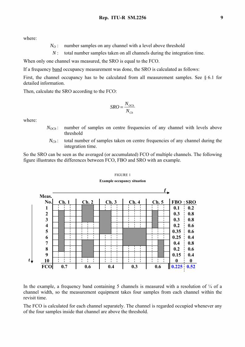
So the SRO can be seen as the averaged (or accumulated) FCO of multiple channels. The following figure illustrates the differences between FCO, FBO and SRO with an example.
FIGURE 1
Example occupancy situation
In the example, a frequency band containing 5 channels is measured with a resolution of ¼ of a channel width, so the measurement equipment takes four samples from each channel within the revisit time.
The FCO is calculated for each channel separately. The channel is regarded occupied whenever any of the four samples inside that channel are above the threshold.
Ch. 1 Ch. 2 Ch. 3 Ch. 4 Ch. 5Meas.
No. FBO SRO
FCO 0.7 0.6 0.4 0.3 0.6 0.225 0.52
1 2 3 4 5 6 7 8 9 10
0.1 0.2 0.3 0.8 0.3 0.8 0.2 0.6 0.35 0.6 0.25 0.4 0.4 0.8 0.2 0.6 0.15 0.4
0 0 t
f

10 Rep. ITU-R SM.2256
The FBO may be calculated for every time slot separately (if desired) which is the shortest possible integration time. To calculate the FBO value, all 20 samples of the measurement have to be taken into account. The FBO for all 10 time slots may either be calculated by averaging the results for each time slot, or by counting all of the 200 samples taken on any frequency that are above the threshold and divide the result by 200 (in the example, 45 out of the 200 samples are occupied, resulting in an FBO of 45/200 = 0.225).
3 Measurement parameters
3.1 Selectivity
One of the most critical aspects when measuring multiple channels or whole frequency bands is to separate emissions from adjacent channels even when their level is quite different. If the measurement bandwidth is too high, a strong emission causes neighbouring channels to appear occupied, too.
FIGURE 2
Correct setting of measurement bandwidth
Figure 2 shows an example of the RF signal of five adjacent channels. Channel 2 and 4 are occupied by signals with different level. The short horizontal lines represent the channel level after evaluation. In this example the measurement bandwidth setting is correct: only the channels 2 and 4 have levels above the threshold.
1
A
Threshold
Channel 2 3 4 5

Rep. ITU-R SM.2256 11
FIGURE 3
Measurement bandwidth setting too wide
In Fig. 3 the measurement bandwidth is too wide: Whereas the occupancy of channel 2 still shows correctly, the strong signal on channel 4 produces phantom occupancies on channels 3 and 5.
It is obvious that the frequency resolution of the measurement equipment must be at least as fine as the (narrowest) channel spacing in the frequency band under investigation. However, depending on the measurement setup, the maximum resolution bandwidth may be much smaller:
– If a standard monitoring receiver is used that is fitted with channel filters, a measurement bandwidth equal to the (narrowest) channel spacing may be used. However, smaller bandwidths are preferred.
– If a sweeping spectrum analyser with Gaussian or CISPR filters is used, the resolution bandwidth should not be wider than 1/10 of the (narrowest) channel spacing in the band.
– If the spectrum is calculated with the FFT method, the maximum distance between adjacent frequency bins is the (narrowest) channel spacing in the band. In this case, however, the frequency bins must lie on the channel centre frequencies. If this cannot be achieved, the distance between adjacent frequency bins must be less than half of the (narrowest) channel spacing in the band.
In bands with frequency hopping spread spectrum (FHSS) systems, the measurement bandwidth may be determined as described above. However, the 99% bandwidth of a single burst in the hopping sequence has to be used as the channel spacing.
3.2 Signal to noise ratio
The sensitivity of the measurement setup should be in the same range as the sensitivity of common user equipment in the band. This ensures that signals detectable for user equipment show with sufficient signal to noise ratio (S/N) in the measurement result in order to separate them from the noise floor. The following minimum S/N may be assumed for this purpose:
– 20 dB for narrowband analogue communications (e. g. private networks).
– 40 dB for wideband analogue communications (e. g. FM broadcasting).
– 15 dB for digital systems (except direct sequence spread spectrum).
Occupancy measurements in bands with direct sequence spread spectrum (DSSS) systems cannot be done with standard measurement equipment because the useful level in the frequency domain is often at or below the noise floor. In these cases the signal to noise ratio of a standard measurement
1
A
Threshold
Channel 2 3 4 5
12 Rep. ITU-R SM.2256
system would not be sufficient to detect these emissions. The presence and level of DSSS emissions can only be measured after dispreading in the code domain.
3.3 Dynamic range
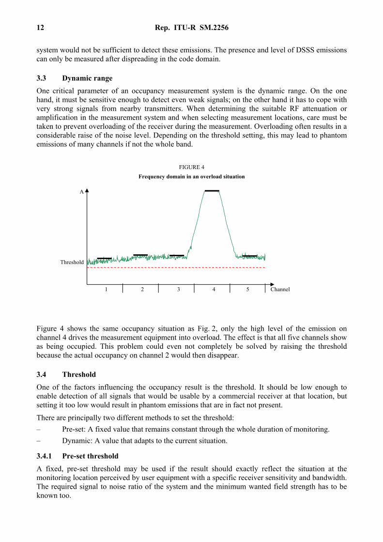
One critical parameter of an occupancy measurement system is the dynamic range. On the one hand, it must be sensitive enough to detect even weak signals; on the other hand it has to cope with very strong signals from nearby transmitters. When determining the suitable RF attenuation or amplification in the measurement system and when selecting measurement locations, care must be taken to prevent overloading of the receiver during the measurement. Overloading often results in a considerable raise of the noise level. Depending on the threshold setting, this may lead to phantom emissions of many channels if not the whole band.
FIGURE 4
Frequency domain in an overload situation
Figure 4 shows the same occupancy situation as Fig. 2, only the high level of the emission on channel 4 drives the measurement equipment into overload. The effect is that all five channels show as being occupied. This problem could even not completely be solved by raising the threshold because the actual occupancy on channel 2 would then disappear.
3.4 Threshold
One of the factors influencing the occupancy result is the threshold. It should be low enough to enable detection of all signals that would be usable by a commercial receiver at that location, but setting it too low would result in phantom emissions that are in fact not present.
There are principally two different methods to set the threshold:
– Pre-set: A fixed value that remains constant through the whole duration of monitoring.
– Dynamic: A value that adapts to the current situation.
3.4.1 Pre-set threshold
A fixed, pre-set threshold may be used if the result should exactly reflect the situation at the monitoring location perceived by user equipment with a specific receiver sensitivity and bandwidth. The required signal to noise ratio of the system and the minimum wanted field strength has to be known too.
1
A
Threshold
Channel 2 3 4 5

Rep. ITU-R SM.2256 13
The threshold is then set to either:
– The minimum wanted field strength.
– The receiver sensitivity plus minimum S/N for the specific radio service.
Care must be taken that the measurement bandwidth matches the bandwidth of the user equipment. If the measurement bandwidth (RBW) is considerably smaller than the occupied bandwidth of the monitored emission (OBW), the threshold must be reduced by 10×log(OBW/RBW).
3.4.2 Dynamic threshold
If the aim of the measurement is to detect as many emissions as possible, regardless of their level, a dynamic threshold that adapts to the current noise level is preferred. The critical part is the reliable detection of the current noise level. In principle, there are several methods:
Direct measurement of the noise level on an unused frequency
This method relies on the availability of a channel (or frequency) near the actual channel (or band) to be monitored that is free of wanted and unwanted emissions. The noise measurement has to be done with the same settings (measurement time and bandwidth) as used for the actual occupancy measurement. The simplest realization of this method is to measure the noise level once and use the result for the whole occupancy measurement. This is only suitable if:
– All channels to be measured (or the whole band, respectively) are relatively close to the frequency of the channel used for the noise measurement.
– The man-made noise level does not change considerably during the monitoring time, or it is lower than the noise level of the measurement system. In bands below 30 MHz this method is generally not advisable because the noise level changes with time due to varying propagation conditions.
If the noise level cannot be assumed to remain constant with time, it is advisable to include an unused channel (or frequency) in the list of frequencies to be measured. This assures that the noise level is measured every revisit time just before the actual occupancy scan starts.
The final threshold of the occupancy measurement must be higher than the measured noise level by a margin of at least 3 to 5 dB. Otherwise short-term peaks in the noise level will result in phantom occupancy.
Direct measurement of the noise level in free time slots
In TDMA systems or analogue systems where a channel is not continuously occupied, the noise level can directly be measured during times at which a channel is not occupied. This method is preferred over the method described above, because the noise measurement is done on the actual channel to be monitored for occupancy. The advantage, especially in occupancy measurements over many channels or a whole frequency band, is that this method is able to consider frequency- and time-dependant noise levels. For example, a strong emission on one channel may produce a rise of the noise level in neighbouring channels due to phase noise of the transmitter.

14 Rep. ITU-R SM.2256
FIGURE 5
Noise level and adaptive threshold
In Figure 5 the noise level on channels 2, 3 and 5 are raised due to a signal on channel 4 (thin red trace). If the unused channel 1 is used to measure the common noise level (thick black dashed lines), the resulting common threshold (thin green dashed line) would be so low that channels 3 and 5 would also show occupied when a signal like in the example is showing up on channel 4. If the noise level is measured on each channel separately (thick black lines), the resulting adaptive thresholds (thin red dashed lines) prevent these phantom occupancies. The sensitivity of the whole measurement is not reduced, because when the signal on channel 4 disappears (thin green trace), the thresholds for channels 2, 3 and 5 would lower down to the common threshold again.
As with the noise level measurement on unused frequencies, the key settings (time, bandwidth) have to be equal to the settings used for the actual occupancy measurement, and the threshold has to be at least 3 to 5 dB above the measured noise level. For the same reasons as mentioned above this method is more accurate if the noise measurement is performed every revisit time just before the actual occupancy measurement.
Calculated threshold
If neither suitable unused frequencies nor times where a channel is known to be unused are available, the threshold can also be calculated from the levels measured throughout one scan. This method, however, works only in frequency band occupancy measurements or occupancy measurements of multiple channels with equal bandwidths.
The so-called “80% method” described in Recommendation ITU-R SM.1753 may be used to calculate the noise level as follows: 80% of all samples representing the highest levels are discarded and the remaining 20% of the samples representing the lower levels are linearly averaged. The result is the noise level. As with the other methods, the final threshold has to be at least 3 to 5 dB above the calculated noise level.
The simplest way to apply this method is to use all measurement samples on all channels (or frequencies) throughout the whole monitoring time for the calculation. This will result in one fixed value for the threshold. Again, this approach can only be used if the noise level does not change with time.
A better adaption of the threshold to the momentary noise level is achieved when only the samples from one scan (or one round through all channels, respectively) are used for the 80% method and the noise level calculation is repeated just before each single scan.
The advantage of the calculation method is that it requires no unused channels or idle times (or knowledge thereof). The disadvantage, however, is that the calculated noise level rises when more channels are occupied with high levels. At these times, measurement sensitivity is lost.
1
A
Common threshold
Channel 2 3 4 5
Adaptive threshold

Rep. ITU-R SM.2256 15
FIGURE 6
Dependency of threshold and occupancy
Figure 6 shows an example of a measurement on five channels at times when only two of them are occupied (green, lower, spectrum trace) and when four channels with high level are occupied (blue, upper spectrum trace). The threshold calculated from the lowest 20% samples is lower when only few channels with low level are occupied. Threshold 2, calculated during high occupancy and high levels, fails to detect the occupancy on channel 2 which means that during these times sensitivity is lost.
3.5 Measurement timing
Especially modern digital systems often operate with short transmission lengths and relatively long times of inactivity (low duty cycle). For a standard occupancy measurement setup it will normally not be possible to capture each single burst of an emission. But this is not necessary because the results will be evaluated on a statistical basis anyway. Provided a large number of samples are taken on one channel/frequency, the duty cycle of interrupted emissions will show up in the result with reasonable accuracy. Unless it is required to investigate the occupancy inside the frame structure of a TDMA system, it is sufficient to mark a particular frequency as occupied at all times where at least one station is transmitting, regardless of how many time slots in a radio frame it uses.
Considering the performance of the measurement system in terms of scanning speed, the time settings for the measurement will normally be a compromise between measurement time on one channel and revisit time. The following considerations may be taken as a guideline when determining the time settings:
– The revisit time should be as short as possible. In any case it has to be shorter than the average transmission time.
– The sample measurement time should be as short as possible. In any case, it should be shorter than a radio frame in a band used by TDMA systems.
When FFT equipment is used, the sample measurement time is equal to the acquisition time. If the minimum requirements for revisit time cannot be fulfilled, either the sample measurement time has to be shortened or the number of channels (or width of the band in FBO) has to be reduced.
Annex 1 provides more detailed information on the dependencies of these parameters.
The following figure illustrates the different times involved in occupancy measurements and their dependencies.
1
A
Threshold 1
Channel 2 3 4 5
Threshold 2

16 Rep. ITU-R SM.2256
FIGURE 7
Timing dependencies
TR = revisit time TM = measurement time Tobs = observation time (TM + overhead)
Transmission A on f1 is assumed to last between t1 and t4 which is the revisit time, although it is actually shorter. Transmission B on f1 is not detected at all because it is outside any measurement window TM. Hence, the revisit time has to be much shorter to increase the detection probability of the short transmissions on frequency f1.
Transmission C on f2 is detected in both measurements because if a peak detector is used the resulting level is independent of whether the emission was present during the whole measurement time TM or only a part of it.
Transmission D on f3 is a TDMA system with a certain duty cycle. Because usually the revisit time of the measurement and the frame duration of the TDMA system are not synchronized, there is a good chance that some bursts remain undetected if the revisit time is longer than the frame length. In this case, when a large number of samples were taken on f3, the likelihood of detecting a burst would be equal to the duty cycle and represent the channel occupancy as well.
To improve the probability of hitting the short emissions from pulsed digital systems such as WLAN and thereby enhancing the confidence level of the result, multiple measurement samples may be taken on one channel before moving to the next channel. This reduces the “blind” times occurring during the processing overhead which includes the time to tune to the next channel. This principle is illustrated in Fig. 8:
TR
TM
Tobs
t1 t2 t3 t4 t
f
f1
f2
f3
A B
C
DD DDD D D

Rep. ITU-R SM.2256 17
FIGURE 8
Timing optimization for short duration signals
3.6 Directivity of the measurement antenna
In most cases data from occupancy measurements should be valid for the location of the monitoring or a specified area around that location. To achieve validity of the results for a circle area around the monitoring location, a non-directional measurement antenna has to be used. This will be the standard setup in most cases.
In the following cases, however, a directional measurement antenna would have to be used:
– The measurement should show occupancy for one specific location and service that also uses directional antennas. Example: The occupancy of the communication network of a railroad company is to be measured. The base stations of the user are positioned along the railroad tracks and bi-directional antennas are used to focus the radio beam on the tracks (see Fig. 9). In this case, the measurement antenna may have the same directivity as the antenna of the base station. The same situation is given when occupancy is measured in a band with point-to-point radio links.
FIGURE 9
Example setup of a railroad communication network
...
...
Base station
18 Rep. ITU-R SM.2256
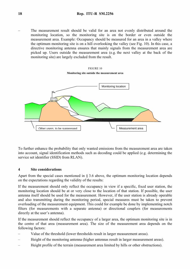
– The measurement result should be valid for an area not evenly distributed around the monitoring location, so the monitoring site is on the border or even outside the measurement area. Example: Occupancy should be measured for an area in a valley where the optimum monitoring site is on a hill overlooking the valley (see Fig. 10). In this case, a directive monitoring antenna ensures that mainly signals from the measurement area are picked up. Users outside the measurement area (e.g. the next valley at the back of the monitoring site) are largely excluded from the result.
FIGURE 10
Monitoring site outside the measurement area
To further enhance the probability that only wanted emissions from the measurement area are taken into account, signal identification methods such as decoding could be applied (e.g. determining the service set identifier (SSID) from RLAN).
4 Site considerations
Apart from the special cases mentioned in § 3.6 above, the optimum monitoring location depends on the expectations regarding the validity of the results:
If the measurement should only reflect the occupancy in view if a specific, fixed user station, the monitoring location should be at or very close to the location of that station. If possible, the user antenna itself should be used for the measurement. However, if the user station is already operable and also transmitting during the monitoring period, special measures must be taken to prevent overloading of the measurement equipment. This could for example be done by implementing notch filters (for measurements with a separate antenna) or directional couplers (for measurements directly at the user’s antenna).
If the measurement should reflect the occupancy of a larger area, the optimum monitoring site is in the centre of that area (measurement area). The size of the measurement area depends on the following factors:
– Value of the threshold (lower thresholds result in larger measurement areas).
– Height of the monitoring antenna (higher antennas result in larger measurement areas).
– Height profile of the terrain (measurement area limited by hills or other obstructions).
Measurement area
Monitoring location
Other users, to be suppressed

Rep. ITU-R SM.2256 19
If the purpose of the measurements is to pick up as many as possible emissions in the monitoring area, a higher monitoring location would be preferred.
If the sensitivity of the measurement system is not higher than that of the user’s equipment in the band, the occupancy as seen by users on the rim of the measurement area may be different from the calculated result. Figure 11 shows an example of a shared company network with two base stations inside the measurement area.
FIGURE 11
Example distribution of stations on a shared company frequency
In Fig. 11, the location of the monitoring vehicle is placed in the centre region of the measurement area. Emissions from base 1 and base 2 are covered. The measurement area is limited to the south by mountains but this is not serious since they also limit the coverage ranges of the mobile network. The sensitivity of the monitoring equipment is equal to that of the base stations and hence the measurement area has the same size as their coverage area.
Emissions from Mobile 1 are detected which is correct in the view of the associated Base 1. However, in the view of Base 2, the frequency appears free although Base 2 is inside the measurement area for which, by definition, the occupancy result should be valid.
Emissions from Mobile 2 are not detected by the monitoring equipment which is correct because Mobile 2 is outside the measurement area. However, the frequency appears to be occupied in the view of the associated Base 2.
The situation in the example leads to inaccurate occupancy results if the expected validity is the whole measurement area. However, on a statistical base the occupancy result is still valid because the likelihood of both effects may be assumed being equal. In our example: the probability of missing a transmission from Mobile 2 may possibly be equal to that of including a transmission from Mobile 1. Therefore, in the view of Base 2, the statistical occupancy is the same as it would be if the monitoring equipment had been placed at the location of Base 2.
Mobile 1
Base 1 Base 2
Monitoring location
Coverage area of Base 1
Coverage area of Base 2
Mountains
Mobile 2

20 Rep. ITU-R SM.2256
To avoid the above mentioned problem, the sensitivity of the monitoring system has to be increased. This can sometimes be achieved by choosing a different, higher monitoring location (in our example on the hill to the south).
5 Measurement procedure
Depending on the measurement task (FBO or FCO) and the nature of the measurement receiver, the actual measurement procedure and the important settings have to be adapted.
Generally, the measurement should record the momentary level detected on each channel or frequency, together with the time. Alternatively, if the actual time is not stored, it is also possible to calculate the actual time of each sample from the beginning of the monitoring and the revisit time, provided it is constant.
For the level measurement, the peak detector must be used. This ensures that even pulsed emissions are captured with their full level.
If the measurement receiver or analyser does not have capabilities to store the results, it has to be connected to a computer that performs this function.
5.1 FCO measurement with a scanning receiver
During the measurement, the receiver repeatedly scans all channels to be measured one by one. For best performance it is necessary to choose an optimum compromise between actual measurement time on one channel and scanning speed (see § 3.5 on timings).
5.2 FBO with a sweeping analyser
During the measurement, the analyser repeatedly sweeps from start to stop frequency. The resolution bandwidth (RBW) is determined by the width of the (narrowest) channels in the band according to the principles in § 3.1. The revisit time is equal to the sweep time. In the setting “auto”, most analysers automatically set the fastest sweep time possible according to the RBW and span.
5.3 FBO with FFT methods
During the measurement, the FFT analyser or wideband receiver repeatedly captures the band to be measured. Ideally, the whole band to be measured can be processed in parallel. However, the maximum spacing of adjacent frequency bins after the FFT must fulfil the requirements explained in § 3.1. This spacing, together with the order of the FFT, determines the maximum bandwidth that can be processed in one shot. Example: The channel spacing and hence the minimum spacing between adjacent frequency bins is 20 kHz (if frequency bins fall on the channel centre frequencies). If the receiver performs a 1k FFT, the maximum bandwidth that can be captured in one shot is 20 kHz × 1024 = 20.48 MHz.
The revisit time and the observation time are equal to the acquisition time plus time needed to perform the FFT.
If the maximum capture bandwidth of the equipment is less than the desired frequency band (either limited by equipment specifications or by the calculation described above), it must be divided into several sub-bands that are processed subsequently. In this case, the revisit time is considerably higher.

Rep. ITU-R SM.2256 21
6 Calculation of occupancy
The principle calculation of frequency FCO, FBO and resource occupancy is already explained in § 2 above. The following therefore only focuses on some special methods to pre-process the measurement data in order to achieve results with reasonable accuracy.
6.1 Combining measurement samples on neighbouring frequencies
Especially when a FBO measurement was performed and the occupancy of certain channels is to be calculated, it is often required to combine measurement results on neighbouring channels to determine the occupancy figure of one channel. This procedure is always necessary when the frequency resolution of the measurement is higher than the channel spacing.
The simplest way is to regard only those measurement samples that are on the frequency nearest to the channel centre frequency and discard all other measurement samples. Figure 12 shows this principle.
FIGURE 12
Simple way of combining measurement samples
The disadvantage of this method is that especially broadband and/or digitally modulated signals may go undetected because their spectrum is noise-like and the spectral density varies in time so that during a momentary measurement, the level of a sample inside the used bandwidth may fall below the threshold. In Fig. 12, the signal on channel 2 is such an example. A similar problem may occur if the centre frequency of a narrowband emission differs considerably from the nominal channel centre frequency.
The best way to combine the measurement samples for the occupancy determination of a channel is to integrate all samples that lie inside the channel boundaries and calculate the channel power. When applying this method, the channel power of the noise has to be the measure that determines the threshold, not the power of a single measurement sample containing noise.
Figure 13 shows an example for this method, using the same measurement samples as in Fig. 12.
1
A
Threshold
Channel 2 3 4 5
used samples
discardedsamples
22 Rep. ITU-R SM.2256
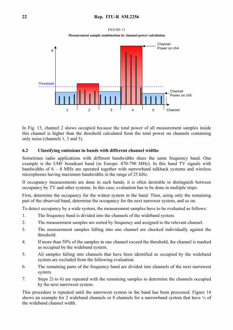
FIGURE 13
Measurement sample combination by channel power calculation
In Fig. 13, channel 2 shows occupied because the total power of all measurement samples inside this channel is higher than the threshold calculated from the total power on channels containing only noise (channels 1, 3 and 5).
6.2 Classifying emissions in bands with different channel widths
Sometimes radio applications with different bandwidths share the same frequency band. One example is the UHF broadcast band (in Europe: 470-790 MHz). In this band TV signals with bandwidths of 6 – 8 MHz are operated together with narrowband talkback systems and wireless microphones having maximum bandwidths in the range of 25 kHz.
If occupancy measurements are done in such bands, it is often desirable to distinguish between occupancy by TV and other systems. In this case, evaluation has to be done in multiple steps:
First, determine the occupancy for the widest system in the band. Then, using only the remaining part of the observed band, determine the occupancy for the next narrower system, and so on.
To detect occupancy by a wide system, the measurement samples have to be evaluated as follows:
1. The frequency band is divided into the channels of the wideband system.
2. The measurement samples are sorted by frequency and assigned to the relevant channel.
3. The measurement samples falling into one channel are checked individually against the threshold.
4. If more than 50% of the samples in one channel exceed the threshold, the channel is marked as occupied by the wideband system.
5. All samples falling into channels that have been identified as occupied by the wideband system are excluded from the following evaluation.
6. The remaining parts of the frequency band are divided into channels of the next narrowest system.
7. Steps 2) to 6) are repeated with the remaining samples to determine the channels occupied by the next narrowest system.
This procedure is repeated until the narrowest system in the band has been processed. Figure 14 shows an example for 2 wideband channels or 8 channels for a narrowband system that have ¼ of the wideband channel width.
1
A
Threshold
Channel 2 3 4 5
Channel Power on ch4
Channel Power on ch5

Rep. ITU-R SM.2256 23
FIGURE 14
Evaluating measurement samples in a band with different channel widths
In Fig. 14, the emission on the narrowband channel 3 will not show up in the first evaluation run for the wideband channels because only 7 out of the 48 samples contained in wideband channel 1 are above the threshold (15%). The signal on wideband channel 2, however, will be detected because 34 of the 48 samples are above the threshold (71%). In the second evaluation run for the narrowband channels, all samples from wideband channel 2 are excluded and will therefore not show up again as four narrowband emissions. The signal on narrowband channel 3, however, will be detected because 7 out of the 12 samples inside this channel are above the threshold (58%).
For this evaluation it is necessary that the frequency resolution of the FBO is at least 4 times higher than the width of the second narrowest channel in the band. If FFT techniques are used, at least 4 frequency bins must fall into the width of the second narrowest channel.
Example: the band to be measured uses channel widths of 25 kHz, 50 kHz and 8 MHz. The frequency resolution for the measurement has to be better than 50/4 = 12.5 kHz. This ensures that we have at least three samples inside each 50 kHz channel which allows the 50%-method to distinguish these signals from the narrowest ones using a 25 kHz spacing.
7 Presentation of results
There are many ways to present the results of occupancy measurements. The optimum way depends on the exact questions that should be answered with the measurement, and on some measurement parameters such as number of channels, bandwidth and duration of monitoring.
The following sections give some examples of result presentation, not necessary being a complete list of all possible ways.
7.1 Traffic on a single channel
The simplest way to present results of FCO measurements is to plot the relative occupancy of the frequency or channel vs. time. For this purpose the samples are averaged over a certain integration time, e.g. over 15 min or 1 h. Shorter integration times improve the time resolution and allow a more detailed analysis of short-term changes in the occupancy. However, if the integration time is lower than the average transmission time, the result becomes difficult to interpret as the occupancy values will most often be either 0% or 100%. An integration time of 15 min is widely used.
Figure 15 shows an example of a traffic plot for one channel.
threshold
A
f 1 narrowband channels
wideband channels
2 3 4 5 6 7 8
1 2
24 Rep. ITU-R SM.2256
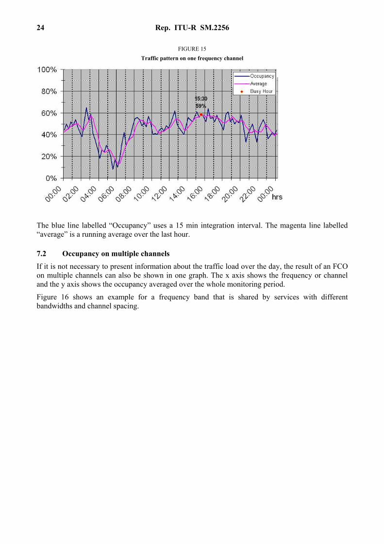
FIGURE 15
Traffic pattern on one frequency channel
The blue line labelled “Occupancy” uses a 15 min integration interval. The magenta line labelled “average” is a running average over the last hour.
7.2 Occupancy on multiple channels
If it is not necessary to present information about the traffic load over the day, the result of an FCO on multiple channels can also be shown in one graph. The x axis shows the frequency or channel and the y axis shows the occupancy averaged over the whole monitoring period.
Figure 16 shows an example for a frequency band that is shared by services with different bandwidths and channel spacing.

Rep. ITU-R SM.2256 25
FIGURE 16
Example occupancy on multiple channels with different widths
The thick red bars in Fig. 16 are occupancies by 8 MHz wide DVB-T signals, the thin blue bars present occupancy by narrowband wireless microphones and talkback links.
This presentation, however, does not provide information on how the occupancy of each channel is distributed over the whole monitoring period. To get that information, an occupancy histogram may be presented. It displays the frequency on the x axis and the time on the y axis. The occupancy value is represented by different colours.
Figure 16 shows an example of such an occupancy histogram (magnified part).

26 Rep. ITU-R SM.2256
FIGURE 17
Occupancy histogram
For better readability, the results in Fig. 17 are integrated over time intervals of about 3 minutes, during which the maximum occupancy value is displayed. The frequency f1, for example, is occupied continuously in all three displayed time intervals (red line = 100% occupancy). Frequency f2, although also present in all three time intervals, is occupied less than 10% (dark green line).
7.3 Frequency band occupancy
One common way to present the occupancy results for a whole frequency band is the spectrogram. It shows the frequency on the x-axis and the time on the y-axis. The level of the emissions is indicated by the colours, usually in the so-called “temperature scale” where blue represents the lowest and red the highest level.
Figure 18 shows an example of such a presentation from a measurement in the 868 MHz ISM band.
FIGURE 18
Frequency band occupancy presentation
Relative occupancy, values below 0.01% are displayed in white
MHz MHz MHz
f1 f2
f1 f2

Rep. ITU-R SM.2256 27
The advantage of this presentation method is that it provides a good, although subjective, impression on the band occupancy at a glance. The disadvantage is that it does not quantify the occupancy on each frequency so that there is no objective value allowing direct comparison with other results. This, however, may be provided by an accompanying diagram showing the relative time during which each frequency was occupied. Figure 19 shows this diagram for the same measurement as in Fig. 18.
FIGURE 19
Objective frequency band occupancy
To get the complete information, both presentations are necessary. From Fig. 18, for example, it can be seen that the frequency 868.35 MHz (f2) was occupied for around 70% of the time. However, we cannot see how the occupancy was spread over the day. It may be a constant emission for 7 out of 10 h of monitoring. Only if we also look at Fig. 17 it becomes clear that the transmitter was present during the whole monitoring period, but it was a TDMA system with an average duty cycle of 70% rather than a constant emission for 7 of 10 h. The occupancy value of 864.5 MHz (f1) is nearly the same (65%), but its distribution over the day is completely different as we can see in Fig. 18.
The total band occupancy (FBO) of 17.31% at the bottom of Fig. 19 is the pure integration of all measurement samples collected on any frequency over the whole monitoring period that had levels above the threshold. In other words, this is the area in Fig. 18 that is not blue. This value should not be mixed up with frequency resource occupancy (SRO) which is considerably higher. When only the spectrogram like in Fig. 17 is presented, the resulting FBO should also be given as a figure in order to provide a means to quantify the result and compare it with others.
Example: There are only four usable channels in the frequency range 865.4 to 867.6 MHz (RFID channels). In Fig. 18 we can see that all four channels are continuously occupied, but with a level below the threshold which is why these emissions don’t contribute to the occupancy in Fig. 18. Had their levels been above the threshold, they would appear as four narrow lines in Fig. 18 and four distinct peaks of 100% in Fig. 19. The FBO value of this frequency range would still be very low because most of the area in Fig. 18 would still be blue. However, the SRO of this frequency range would be 100% because all available resources (4 channels) are continuously occupied.
The information in Fig. 18 is somewhat similar to Fig. 16 also displaying the results of a band measurement. However, both diagrams have a different frequency resolution: Fig. 16 shows one vertical bar per frequency channel (which even may be of different widths), whereas the horizontal
f1 f2

28 Rep. ITU-R SM.2256
resolution in Fig. 19 is the frequency resolution used for the measurement (independent of the channel width). Therefore, the band occupancy (FBO) cannot be directly taken from Fig. 16.
7.4 Spectrum resource occupancy
As an example of utilizing the results of spectrum resource occupancy measurements, a long-term measurement of two different frequency bands allocated to FM broadcasting links was carried out using fixed and mobile monitoring equipment as illustrated in Fig. 20.
FIGURE 20
Used fixed (left) and mobile (right) monitoring system to measure the spectrum occupancy
The FM broadcasting links are used to transport programme contents from a remote production site to the nearest studio, between studios, or from the studio to a transmitter site.
Because the spectrum usage was expected to be very low, the results should justify a reallocation of the 900 MHz range to other communication services. Figure 21 shows the occupancy results for each available channel in both bands separately.
FIGURE 21
Measurement result of the FM broadcasting links service (942~959 MHz, 1 700~1 710 MHz)
The calculated SRO of the lower band was 3.85% and it was less than 1% in the higher band. This result led to the decision to combine all FM broadcast links services in the upper band, making the lower band available to the mobile communication service which is growing fast.

Rep. ITU-R SM.2256 29
7.5 Availability of results
The results should be made available to all those are working with occupancy results, either in the frequency planning or licensing and enforcement sections. It is preferable to publish them on a website of the intranet of the organization or even in the internet.
In case the organisation is using a computerized spectrum management and/or licensing programme, the results should be available in the monitoring part of the relevant data base, preferably via an automated data interface.
Neighbouring Administrations may be interested in exchanging occupancy data, especially concerning regions near the country borders, to assist in frequency assignments. In such cases it is important to use a unique and unambiguous format that allows correct interpretation of the data the cooperating parties deliver to each other. As an example, Recommendation ITU-R SM.1809 “Standard data exchange format for frequency band registrations and measurements at monitoring stations” recommends the use of comma-delimited ASCII (comma separated value – CSV) file format for this purpose when exchanging occupancy data. Most common database and spreadsheet programs can read this format.
8 Special occupancy measurements
8.1 Frequency channel occupancy in frequency bands allocated to point-to-point systems of fixed service
Some terrestrial point-to-point systems of fixed service (for example, fixed WiMAX, radio-relay communications, interconnection of base stations for cellular radio systems etc.) use directional links. In this case the detection of an emission at one site using omni-directional antennas results in a certain amount of channel occupancy at this site only (see Fig. 22). But it doesn’t mean that this channel is not usable for other links, even if signal level exceeds threshold level. Several fixed links can use the same channel without creating any harmful interference to each other.

30 Rep. ITU-R SM.2256
FIGURE 22
Monitoring of frequency channel occupancy in frequency bands allocated to point-to-point systems of fixed service
However, results of a frequency channel occupancy measurement at the site of the monitoring unit using omni-directional antennas shows the frequency channel as occupied even if there is an emission from a single link only (for example, Link A).
In this case, the standard occupancy measurement setup will normally not provide the desired information. Depending on the purpose of the occupancy measurement, the following cases may be distinguished:
– If the measurement is done to find available frequencies for a proposed new fixed link, the measurement should be done with a directional antenna. The monitoring unit has to be placed at both locations of the proposed new link.
– If the measurement is done to provide an overview of the utilization of the frequency band, regardless of the exact location, the measurement can be done with an omni-directional antenna at the location indicated in Fig. 22, where a maximum of links can be received.
8.2 Separation of occupancy for different users in a shared frequency resource
If field strength is recorded, additional information can be extracted from the measurement.
The left plot in Fig. 23 is a commonly used way to present the occupancy with a resolution of 15 min, normally with only one curve. The red curve in the left plot represents the total occupancy caused by all users on that channel. The green curve is the occupancy caused by the station received with about 49 dB(μV/m) (see right side plot) and the blue curve is the occupancy caused by all the other users, in this case the second user received with about 29 dB(μV/m).
The plot in the middle represents the received levels over time. Only received levels above the threshold level (here: 20 dB(μV/m)) are evaluated.
Link C
Link B
Mobile monitoring unit site

Rep. ITU-R SM.2256 31
The right plot shows the statistical distribution of the received field strength levels. In this example 49 dB(μV/m) has been measured about 380 times in a 24 h period, 50 dB(μV/m) about 350 times etc.
FIGURE 23
Enhanced processing of occupancy data
8.3 Spectrum occupancy measurement of WLAN (Wireless Local Area Networks) in 2.4 GHz ISM band
The 2.4 GHz ISM (Industrial, Scientific and Medical) band is mainly used for Wireless LAN (IEEE 802.11b/g/n), Bluetooth, Zigbee and DECT (in North America) without requiring an individual license. As the use of wireless internet increased rapidly in recent years, there are often a number of WLAN APs (access points) and mobile stations on the same channel.
Because the channel spacing of 5 MHz with a usual occupied bandwidth of up to 20 MHz, channel overlap exists and neighbouring channels cannot be used at the same location without any interference potential.
Figure 24 shows the power over time of WLAN channel 1.
FIGURE 24
Power vs. time graph of WLAN ch.1 (Freq. = 2.412 GHz, BW = 5 MHz)
0 2 4 6 8 10 12 14 16 18 20 22 24 0 2 4 6 8 10 12 14 16 18 20 22 24
100
80
60
40
20
0
Occ
upan
cy (
%)
E (
dB(
V/m
))μ
80
60
40
20
Hours Hours
350
300
250
200
150
100
50
030 70 80 90 10040 50 60
Nu
mbe
r of
occ
uren
ce
E (dB( V/m))μ

32 Rep. ITU-R SM.2256
For some purposes it is useful to obtain occupancy figures only for a specific user on a frequency, for example to identify interference sources or to recommend channel changes in order to use the available band most efficiently. In the 2.4 GHz WLAN band, this can be achieved by using standard user equipment as a receiver and publicly available scanning software. Figure 25 shows an example output of such a setup where channel 11 is occupied by 4 different Access Points.
FIGURE 25
Example of APs List
A second possible reason to identify the MAC address of each transmission is that this method is also capable of separating WLAN emissions from other ISM emissions in the same band (e.g. Bluetooth, Zigbee, DECT).
8.4 Determining the necessary channels for the transition from analogue to digital trunked systems
Currently, many formerly analogue systems are transferred to digital. If an analogue mobile network undergoes this transition, a digital trunked network may be the solution. However, whereas an analogue network needs a separate frequency for each communication channel, trunked networks organize the frequency resources dynamically according to current traffic, thereby getting along with far less frequency channels. An occupancy measurement of the analogue network during peak times can determine how many channels would be needed in a trunked network to manage the traffic with the same quality of service.
As an example, occupancy measurements of an analogue police network were made during major events where peak traffic was expected. This network is to be transferred into a TETRA network. The question was raised how many TETRA channels would be needed without noticeable degradation of the quality of service.

Rep. ITU-R SM.2256 33
The current analogue police network uses 60 channels, spread over a frequency range with a channel spacing of 20 kHz. The setup for the occupancy measurement was able to measure all channels with a revisit time of 1 s. For each round through the channels, it was counted how many of them were occupied simultaneously. The result is shown in Figure 26.
FIGURE 26
Number of channels occupied at the same time
It can be seen that a maximum of 12 channels are occupied at the same time. To manage this amount of traffic, 3 TETRA channels would be necessary since TETRA is able to carry 4 communication channels on one frequency using TDMA techniques.
Although this already gives a big improvement in terms of spectrum efficiency, the question may be raised whether it is necessary to provide capacity for a peak traffic situation that may only occur once a year for a short moment. To answer this question it is necessary to evaluate the occupancy measurement in different ways.
Sorting the scans over the band by the number of occupied channels in each scan results in a row starting with the number of scans where no channel is occupied, then the number of scans with 1 occupied channel and so on. This result may be visualized in a graph such as in Fig. 27.
Cha
nnel
s us
ed c
oncu
rren
tly
Time

34 Rep. ITU-R SM.2256
FIGURE 27
Number of scans with concurrent occupied channels
It can be seen that the case where 12 channels are occupied occurred only 2 times during the whole monitoring period. However, we cannot say whether this occupancy situation occurred once for a two-second period or twice for a period of one second each. To visualize this also, a 3-D diagram may be drawn where the duration of occupancy of a certain number of concurrent channels used is combined. The probability that each situation occurs is shown on the y axis.
1
10
100
1000
10000
100000
0 1 2 3 4 5 6 7 8 9 10 11 12number of channels used in parallel
scan
s

Rep. ITU-R SM.2256 35
FIGURE 28
Probability and duration of concurrently used channels
From this figure we can see that the situation of 12 and even 11 concurrently occupied channels occurs only for a maximum time of 1 s. This means, if a future TETRA network would provide only 10 communication channels, the 11th user at that moment would have to wait for a maximum of one second to get access to the network. Since this is certainly acceptable, 10 TETRA communication channels would be sufficient. Using this evaluation of the occupancy measurement result together with the user’s tolerable access delay allows determining the necessary number of TETRA channels while maintaining maximum spectrum efficiency at minimum costs.
8.5 Estimation of RF use by different radio services in shared bands
Some frequency bands are allocated to different radio services having the same or similar RF properties. Many sub-bands of the HF frequency range are examples for this situation. If signal identification methods are available during the occupancy measurement, the results may be presented separately for each of the services in a band.
9 Uncertainty considerations
The measurement uncertainty depends on various factors such as the revisit time, number and length of transmissions on a channel, number of measurement samples, monitoring duration, whether systems with pulsed emissions (TDMA) are measured, and even the actual occupancy
1 2 3 4 5 6 7 8 9
12
34
56
78
910
1112
0
0,001
0,002
0,003
0,004
0,005
0,006
rela
tive
prob
abili
ty o
f situ
atio
n
seconds in which n channels are occupied concurrently
num
ber o
f cha
nne.
.

36 Rep. ITU-R SM.2256
value itself. Some of these parameters have a complex dependency. Calculations of these parameters and details about their dependencies can be found in Annex 1 to this report.
It should be noted that, although the measurement results may be regarded as accurate, they are valid only for the location and time of the measurement. However, they are normally used to “predict” the occupancy for future times or different locations/areas. The accuracy of this “prediction” strongly depends on the situation and/or service in question: The occupancy of a public phone mobile network will usually be somewhat constant during normal working days, so a measurement taken on one day may be used to assess the usage of the band during all of these days. On the other hand, the occupancy of a shared company channel strongly depends on the actual activity of all users which may differ considerably from day to day, so a measurement taken on one working day may not be usable at all to assess the average traffic load on that channel.
10 Interpretation and usage of results
10.1 General
The results of spectrum occupancy measurement on a specific frequency band may be used to establish frequency allocations and assignment policies gaining an effective spectrum use and economic value of the spectrum resource. For example, they may lead to the re-allocation of frequency bands.
Performing occupancy measurements repeatedly under the same measurement conditions can show trends in the usage of spectrum resources. This may provide valuable information for the future allocation of spectrum to certain services.
10.2 Interpretation of occupancy results in shared channels
As mentioned in the definition of occupancy time, the result provided by the monitoring services should reflect the true occupancy of a channel as accurate as possible. This includes the fact that a channel used by TDMA systems does not already show 100% occupancy when just one station is using it. This makes it necessary for the spectrum management or licensing section to interpret the results depending on the purpose of the occupancy measurement.
Example: If the purpose of an occupancy measurement in a frequency band assigned to a certain network is to check which traffic channels are in use and are therefore not available to other systems at the particular location, all frequencies showing an occupancy typical for that network may be regarded as “full”.
10.3 Using occupancy data to assess spectrum utilization
So far, spectrum occupancy was related to a specific location or the area around the monitoring location only. Sometimes, information about the occupancy of a resource over a large territory (e.g. the whole country) is of interest. To characterize this, Recommendation ITU-R SM.1046-2 defines a spectrum utilization factor, U, as the product of the bandwidth B, the geometric (geographic) space (usually area) S, and the time T during which the spectrum resource is denied to other potential users:
U = B · S · T
The spectrum utilization factor is therefore a three- dimensional parameter: frequency × space × time. The formula is non-linear and only valid for one particular application during a measurement. When a “spectrum utilization map” of a larger area is requested, the most efficient way is to

Rep. ITU-R SM.2256 37
perform a spectrum occupancy measurement using mobile monitoring vehicles. Together with the current occupancy situation, the geographic coordinates are stored so that the occupancies taken in geographic rectangles of a defined size can be averaged. The result may be presented in a map where the different spectrum utilization values are represented by different colours. Figure 29 provides an example of such a spectrum utilization map.
FIGURE 29
Example spectrum utilization map
11 Conclusions
Taking into account that the current Recommendation ITU-R SM.1880 describes only the basic procedures, the various examples in this Report have shown that measurement and especially evaluation of occupancy may be quite a complex task. Thorough knowledge of the radio services and particularly an in-depth analysis of the goal of the measurements are indispensable to specify the measurement and evaluation methods appropriate.
High utilization
low utilization

38 Rep. ITU-R SM.2256
Annex 1
Probabilistic approach to spectrum occupancy measurements and relevant measurement data handling procedures
A Preface
This Annex covers in detail the dependencies of measurement parameters such as revisit time, required number of samples and their influence on measurement accuracy and confidence level. The approach uses mathematical calculations applicable in circumstances such as:
– Unevenly timed measurement samples.
– Measurement delays when detecting used channels.
– Equipment being used for different measurement tasks simultaneously, thereby not being able to dedicate all time to the occupancy measurement task.
The relevance and application of the principles of this annex may be decided on a case-by-case basis, depending on the aim of the measurement, required accuracy and/or confidence level and capabilities of the measurement equipment.
A1 General description of the approach
The Annex describes a probabilistic method used by some administrations for the prediction of the influence of parameters of spectrum occupancy measurement procedure on the statistical confidence of the values obtained. Recommended approach defines the requirements for measuring equipment and for relevant data handling process that allows to determine spectrum occupancy for a large set of radio channels on the stipulated time interval with the desired accuracy and statistical confidence. The findings described in this Annex have already found their practical implementation showing good results [А.1].
The probabilistic approach described below in detail is based on the definition of spectrum occupancy as the probability that, at a randomly selected moment in time, a radio channel, frequency band or other frequency resource being analysed will be in use for the transmission of information [A.2]. Its description is presented in [A.3].
This Annex relates primarily to issues related to the determination of accuracy and statistical confidence of measurements. For the sake of clarity, it is concentrated on the measurement of radio channel occupancy, although obtained results cover other spectrum resources as well.
Channel occupancy may change through time. To monitor the changes, the time axis has to be divided into a set of integration time periods. These integration time periods shall be of fixed duration, usually between 5 and 15 min. The occupancy value has to be calculated for each integration time, and the overall duration of monitoring TT will as a rule be the aggregate of the integration time periods.
From a statistical point of view on the basis of the limited observations we only can estimate the occupancy and it is true for any measurements and data handling procedures. This estimation due to the influence of random factors may differ from the true value of occupancy, which can be determined only in case of continuous monitoring of the channel in question. So, in this Annex a distinction is made between true values of occupancy and its estimations obtained by calculations. Therefore, the term “occupancy” here makes sense somewhat different from that used in the main part of the Report. In the aim of distinction from abbreviation “FCO” used in the main part of the Report, in this Annex it will be used general term “spectrum occupancy (SO)” in relation to the true

Rep. ITU-R SM.2256 39
value of occupancy and the term “spectrum occupancy calculation result(s) (SOCR)” as a practical result of relevant data handling. In fact, SOCR is also the result of spectrum occupancy measurement because it is actually determined entirely on the basis of calculations.
A2 Concept of spectrum occupancy
A2.1 Spectrum occupancy as a statistical concept
As it was mentioned above, from the statistical point of view spectrum occupancy means the probability that, at a randomly selected moment in time, a radio channel, frequency band or other frequency resource being analysed will be in use for the transmission of information.
For the analysis of spectrum occupancy it is considered that only two channel states are possible: “occupied”, whereby the signal level in the channel exceeds a selected detection threshold, and “free”, whereby the signal level in the channel is small. Spectrum occupancy SO is determined by the probability of its being in the occupied state.
FIGURE A1
Definition of the concept of radio channel occupancy
Detection threshold for determining channel
activity
t
U(t)
TI
2tΔ1tΔ VtΔ
Figure A1 shows an example of the possible change over time in the level U(t) of a signal in a channel over an integration time TI. The probability that an occupied signal state will be detected at a randomly selected sample point on the time axis will be equal to the ratio of the aggregate duration of occupied state intervals Δt1, Δt2 …Δtv to the total integration time TI. Thus, spectrum occupancy over this integration time is expressed by:
(A1)
where:
SO : true value of occupancy over the current integration time
TI : duration of the integration time
V : number of occupied state intervals during the integration time TI
Δt1, Δt2 …Δtv : duration of occupied state intervals in the radio channel in case of its continuous monitoring.
1
V
v Iv
SO t T=
= Δ
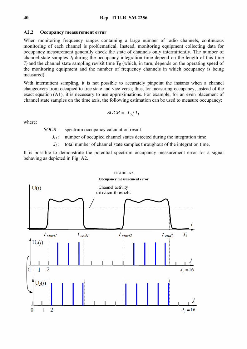
40 Rep. ITU-R SM.2256
A2.2 Occupancy measurement error
When monitoring frequency ranges containing a large number of radio channels, continuous monitoring of each channel is problematical. Instead, monitoring equipment collecting data for occupancy measurement generally check the state of channels only intermittently. The number of channel state samples JI during the occupancy integration time depend on the length of this time TI and the channel state sampling revisit time TR (which, in turn, depends on the operating speed of the monitoring equipment and the number of frequency channels in which occupancy is being measured).
With intermittent sampling, it is not possible to accurately pinpoint the instants when a channel changeovers from occupied to free state and vice versa; thus, for measuring occupancy, instead of the exact equation (A1), it is necessary to use approximations. For example, for an even placement of channel state samples on the time axis, the following estimation can be used to measure occupancy:
Io JJSOCR =
where:
SOCR : spectrum occupancy calculation result
JO : number of occupied channel states detected during the integration time
JI : total number of channel state samples throughout of the integration time.
It is possible to demonstrate the potential spectrum occupancy measurement error for a signal behaving as depicted in Fig. A2.
FIGURE A2
Occupancy measurement error

Rep. ITU-R SM.2256 41
The top diagram U(t), which shows the continuous change in the signal level in the channel over time, corresponds to a true value SO ≈ 50%. The two following diagrams illustrate occupancy measurement with the same number of samples JI, but with a slight “mismatch” in terms of the points as from which the time is counted. Comparing diagrams U1(j) and U2(j), it can be seen that the measured occupancy value in the first case will be SOCR1 = 7/16 ≈ 43.75% and in the second case SOCR2 = 9/16 ≈ 56.25%.
It is obvious that:
1) In addition to the first and second diagrams presented, other options are also possible with different placements of measurement start points, in which there will be exactly eight instances of channel activity over the integration time, giving a precise occupancy estimate of SOCR = 8/16 = 50%.
2) Increasing the number of samples JI reduces the potential spread of measurement results and makes it possible to guarantee negligible error irrespective of the start time selected.
Thus, the spectrum occupancy calculation results SOCR are random values, and the quality of the occupancy measurements has to be analysed from a statistical standpoint.
A2.3 Accuracy and confidence level of occupancy measurement
For the reasons considered under § A2.2 above, radio channel occupancy measurement is in practice subject to error. It may be shown (see, for example, [A.3]) that the occupancy measurement error in a specific r-th test case (SOCRr – SO) is a random value with, as a rule, a close-to-normal distribution. Error magnitudes may vary very significantly in the different tests. This means that conditions have to be imposed on the quality of occupancy evaluation from the standpoints of accuracy and confidence.
Confidence PSOC is the probability that the calculated occupancy SOCR will differ from the true value SO by no more than the permissible absolute error ΔSO.
{ }SOSOC SOSOCRPP Δ≤= – (A2)
where:
PSOC : confidence level of the occupancy measurement
SOCR : calculated occupancy value obtained for the current integration time
SO : true value of occupancy over the integration time
ΔSO : permissible absolute measurement error tolerance corresponding to half of the confidence interval.
Accuracy requirements are also often expressed in terms of the permissible relative measurement error tolerance δSO, which is linked to the permissible absolute error by the equation:
SOSOSO Δ=δ (A3)
Whether accuracy requirements should be expressed in terms of absolute or relative error depends on what kind of magnitudes of occupancy values (small or large) it is more important to measure in practice.
Limitation of the permissible relative measurement error imposes higher demands (small confidence interval) on measurement accuracy in radio channels with a low occupancy and relaxes the demands on measurement accuracy for channels with high occupancy. For example, taking a typical value δSO = 10%, for a channel with an occupancy SO = 2% values in the range 1.8% ≤ SOCR ≤ 2.2% will

42 Rep. ITU-R SM.2256
be considered as falling into the confidence interval (whose size is 0.4%), whereas for an occupancy SO = 20% the confidence interval will increase up to 4%. For a channel with an occupancy SO = 92% any values will be considered as the acceptable ones within the wide range 82.8% ≤ SOCR ≤ 100%.
When the permissible absolute measurement error is limited, the size of the confidence interval is independent of the actual channel occupancy. In particular, with the value of ΔSO = 0.5% that is recommended for use in practice, the size of the confidence interval remains at 1% for both low-occupancy and high-occupancy channels. This corresponds to a very rough estimate for channels with low occupancy, and a very accurate estimate for channels with high occupancy. For instance, for an occupancy SO = 92%, values lying in the range 91.5% ≤ SOCR ≤ 92.5% are considered acceptable.
As regards the required confidence levels, values in the range 90-99% are generally recommended for use in practice. In this Annex, a value of PSOC = 95% will henceforth be used as a basis.
A2.4 Parameters affecting the statistical confidence of occupancy measurement
A2.4.1 Pulsed and lengthy signals and signal flow rate.
The statistical properties of occupancy calculation results depends on the typical duration of the signals in the radio channel analysed. If the signal duration is larger than the revisit time, such signals can’t be missed and the state-changeover points tend to fall at different, independent intervals relative to the samples. The signals with a duration shorter than the revisit time are registering only sometimes, and the statistical properties of occupancy calculations for the channels with these signals are significantly different. Of course, in practice the edge between these types of signals is rather thin. Lengthy signals are considered to be those whose duration Δtv is at least one thousandth of the integration time, i.e. meeting the condition Δtv ≥ 10−3 · TI; pulse signals are those with a duration Δtv < 10−4 · TI.
It is shown in [A.3] that the accuracy and confidence level of occupancy measurements for lengthy signals is strongly dependent on the number of transmissions (or the number of changeovers in state of the channel) within the integration time. Section A4 of this Annex also contains examples showing that for different numbers of signals detected during the integration time, the required number of samples for a confident occupancy measurement may vary by around an order of magnitude. In case of occupancy measurements for the channels with lengthy signals the concept of signal flow rate can be useful.
Signal flow rate λ is the average number of signals present in the channel over a given time period. For example, if, in a particular channel, 140 transmission sessions are observed on average within every one-hour time period, then the signal flow rate for that channel will be λ = 140 signals/hour. Recommendations regarding the consideration of signal flow rate in occupancy measurement will be provided in § A3.1.3.
It should be borne in mind that the signal flow rate in a radio channel λ for different time periods may vary significantly. This means that the variation in signal flow rate has to be tracked during the course of the measurements and the average number of signals expected within the occupancy integration time has to be adjusted accordingly.

Rep. ITU-R SM.2256 43
A2.4.2 Relative instability of revisit time
There are a number of reasons that might lead to an uneven placement of channel state samples on the time axis:
– When measuring occupancy in channels with significantly different signal flow rates, the required number of samples may vary five or tenfold. Strictly cyclical sampling of the state of such channels is ineffective, and changing to a flexible channel sampling procedure will lead to an uneven placement of samples on the time axis.
– State-of-the-art monitoring systems are extremely fast and, when the number of channels to be monitored is small, are capable of undertaking occupancy measurement data collection and other monitoring tasks in parallel, but when equipment resources are divided up in this way the placement of samples on the time axis also becomes uneven.
There may also be other reasons causing instability of the revisit time between samples.
Let the times tj (1 ≤ j ≤ JI) correspond to the real placement of samples on the time axis. The intervals TR j between samples:
11– 1, JjttT jjRj ≤<−= (A4)
in practice experience random fluctuations in relation to the mean value of the revisit time:
IIR JTT = (A5)
where:
TI : duration of the integration time
JI : number of channel state samples within the integration time.
The relative instability of the revisit time is called δT, and is determined by the maximum deviation of the interval between samples from its mean value. It is expressed by:
{ } IRRjjj
JjTTttT ≤<=δ 1,––max 1– (A6)
where:
δT : relative instability of the revisit time
tj : real sampling times
TR : mean value of the revisit time, derived from (A5)
JI : number of samples within the integration time.
A2.4.3 Use of lock-in and lock-out measuring systems for occupancy measurements
In the case of unstable revisit times, the confidence level of occupancy measurements depends also on whether the measuring system used is a lock-in or a lock-out system.
Lock-in systems feature is the use of a generator, which determines a kind of ideal grid of sampling points on the time axis. The real channel state samples may be displaced in relation to the nodes of this ideal grid, but for points located in the different sections of the integration time these displacements are independent.
Lock-out systems are understood to be ones in which there is no time grid, measurement is carried out on the basis of approximately equal revisit times, and the displacement of any point affects the placement on the time axis of all subsequent sampling points.

44 Rep. ITU-R SM.2256
For short time intervals, the difference in the systems’ behaviour is not too noticeable, but for a typical integration time duration TI of hundreds of seconds, the differences in the placement of channel state samples on the time axis become significant and have a noticeable impact on the statistical characteristics of occupancy measurement in radio channels with lengthy signals. Recommendations for achieving measurement confidence for lock-in and lock-out systems will be given in the next sections. Statistically confident measurement of occupancy in channels with pulse signals requires a much larger number of samples in the integration time, although for pulse signals the difference between lock-in and lock-out systems becomes negligible.
A3 Measuring procedures
A3.1 Recommendations for measuring occupancy with lock-in measuring systems
A3.1.1 Data collection
To measure occupancy, one must at the very least determine for each integration time the number JO of occupied channel state samples.
Where there are predominantly lengthy signals in the channel, in order to ensure measurement confidence, information is also required on the signal flow rate λ. When such information is lacking, it is worthwhile to track the grouping of occupied and free states so as to determine a quantity Vr of signals detected in the channel in the r-th integration time. The number of signals detected Vr is considered to be equal to the number of changeovers from free to occupied state and vice versa.
A3.1.2 Occupancy measurement rule
The rule for the measurement of occupancy was already discussed earlier in § A2.2, and takes the form:
Io JJSOCR = (A7)
where:
SOCR : spectrum occupancy calculation result
JO : number of occupied channel states detected during the integration time
JI : total number of channel state samples throughout of the integration time.
A3.1.3 Selecting the number of samples
Requirements for measuring equipment and for relevant data handling processes of occupancy calculations will be different for channels with lengthy and pulsed signals. For channels with lengthy signals, it is determined first of all by the quantity of signals within the integration time. For channels occupied by pulsed signals, confidence depends on the value of radio channel occupancy itself.
For radio channels with lengthy signals, the number of samples required to achieve a confidence PSOC with a permissible absolute measurement error tolerance ΔSO may be calculated as follows:
( )
2
06.1 2
min
TVxJ
avr
SO
pI
δ+⋅⋅
Δ= (A8)
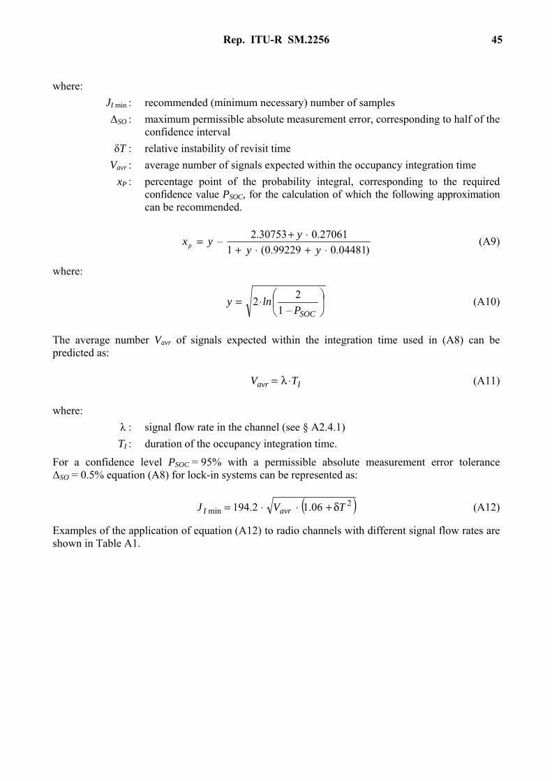
Rep. ITU-R SM.2256 45
where:
JI min : recommended (minimum necessary) number of samples
ΔSO : maximum permissible absolute measurement error, corresponding to half of the confidence interval
δT : relative instability of revisit time
Vavr : average number of signals expected within the occupancy integration time
xP : percentage point of the probability integral, corresponding to the required confidence value PSOC, for the calculation of which the following approximation can be recommended.
)04481.099229.0(1
27061.030753.2–
⋅+⋅+⋅+=
yy
yyxp (A9)
where:
⋅=SOCP
lny–1
22 (A10)
The average number Vavr of signals expected within the integration time used in (A8) can be predicted as:
Iavr TV ⋅λ= (A11)
where:
λ : signal flow rate in the channel (see § A2.4.1)
TI : duration of the occupancy integration time.
For a confidence level PSOC = 95% with a permissible absolute measurement error tolerance ΔSO = 0.5% equation (A8) for lock-in systems can be represented as:
( )2min 06.12.194 TVJ avrI δ+⋅⋅= (A12)
Examples of the application of equation (A12) to radio channels with different signal flow rates are shown in Table A1.

46 Rep. ITU-R SM.2256
TABLE A1
Recommended number of samples for a channel with lengthy signals required to achieve an absolute occupancy measurement error tolerance ΔSO of no more
than ±0.5% with a confidence of PSOC = 95% for measurements with a relative instability of revisit time δT ≤ 0.5
Signal flow rate in the channel λ (average number of signals observed in the occupancy integration time), not exceeding:
Recommended number of samples
10 703
30 1 217
50 1 572
100 2 223
300 3 850
500 4 970
NOTE – The data in the right-hand column of the table are given under the assumption of usage of equation (A7) for lock-in measuring systems, or equation (A19) for lock-out measurements.
According to the data in Table A1, for channels with lengthy signals and a low occupancy (hence, also a low signal flow rate λ), statistically reliable measurement results are obtained with a number of samples JI < 103, which diverges from the information given in [A.4], [A.5]. The discrepancies are explained by the fact that, in Table A1 shown here, the data were obtained with a limitation not on the relative but on the absolute measurement error, which does not assume any narrowing of the confidence interval for cases of low radio channel occupancy (see § A2.3). Occupancy measurement error arises from the lack of accurate data on the instants when the radio channel changes over from occupied to free state and vice versa [A.3]. Thus, the more such changeovers there are during the integration time, the greater the potential measurement error. It is precisely for this reason that, in order to achieve statistical confidence in the results, it is necessary in equation (A7) to increase the number of samples not as the occupancy value increases but as the average number of signals expected in the channel over the integration time increases. In this way, by setting the permissible absolute error tolerance ΔSO for both channels with low occupancy and channels with high occupancy but not many changes in state (such as those occupied by broadcasting stations), it is sufficient to carry out only between 632 and 703 revisits. Only for channels displaying a large number of changes in state over the integration time does the required number of samples become significant.
If the signal flow rate λ over the occupancy integration time is not previously known, then it is recommended to stipulate a value selected with some margin. To adjust the signal flow rate in the course of the measurements, it is recommended to use the equation:
( ) ( )1)1( ++=+ wVw rrr λλ (A13)
where:
λ(r+1) : flow rate expected in the next integration time
λr : flow rate for the current (elapsed) integration time
Vr : number of signals that has been determined in the current integration time
w : weighting coefficient determining the response time of the adaptation procedure, usually selected within the range 5 ≤ w < 20.

Rep. ITU-R SM.2256 47
To start the evolution according to equation (A13) an initial value λ0 is needed which is usually unknown a priory. It is advisable to choose a maximum among all values expected within the given frequency range, which corresponds to the worse case.
For channels with pulsed signals, calculation (A7) also gives an unbiased occupancy measurement but it requires significantly more samples to achieve a confidence PSOC with a permissible absolute measurement error tolerance ΔSO . We can calculate the necessary number of samples JIT as:
2
min )–1(
Δ
⋅⋅=SO
pI
xSOSOJ (A14)
where:
JI min : recommended (minimum necessary) number of samples
SO : radio channel occupancy for the channel with pulse signals
xP : percentage point of the probability integral (see (A9))
ΔSO : maximum permissible absolute measurement error, corresponding to half of the confidence interval.
For a confidence level PSOC = 95% and a maximum permissible absolute measurement error ΔSO = 0.5% equation (A14) can be expressed as follows:
)–1(664153min SOSOJ I ⋅⋅= (A15)
With pulse-type signals, the confidence of the calculation (A7) is determined by the occupancy value itself and is practically independent of instability of samples placement along the time axis and also of whether the measurements involved are of the lock-in or lock-out variety. The application of equation (A15) to radio channels with different occupancies is illustrated in Table A2.
A3.1.4 Effect of incorrect choice of number of samples on the confidence level of the occupancy measurement
Reducing the number of samples JI by a factor of K in relation to what is recommended in Tables A1 and A2 will reduce reliability, or widen the confidence interval proportionally with K.
Let us assume, for example, that we need to measure the occupancy of a radio channel with a signal flow rate of no more than 50 signals within the integration time. From the last column in Table A1, we see that the recommendation in this case is to sample the channel state 1 572 times. Complying with this recommendation, the occupancy calculation (A7) will deviate by no more than ΔSO = 0.5% from the real value, with a confidence level of PSOC = 95%. If we now assume, on the other hand, that the system is actually capable of taking only 393 channel state samples over the integration time, i.e. four times less than the recommended number, then on average the occupancy will as before be measured accurately, but the range within which the real occupancy value will occur with a confidence level of 95% is increased fourfold to ±2% either side of the measurement result.
An inadequate number of samples JI may also be observed when data collection for the occupancy calculation is curtailed prematurely. In such cases, the occupancy calculation (A7) remains unbiased but the confidence level of the results is diminished similarly to the example discussed above.

48 Rep. ITU-R SM.2256
TABLE A2
Recommended number of samples for a channel with pulse signals, required to achieve an absolute occupancy measurement error tolerance ΔSO of no
greater than ±0.5% with a confidence of PSO = 95%
Radio channel occupancy SO
(%)
Recommended number of samples, JI
Recommended revisit time, TR (ms)
for TI = 5 minutes for TI = 15 minutes
5 7 300 41.1 123.2
10 13 830 21.7 65.0
20 24 586 12.2 36.6
35 34 960 8.6 25.7
50 38 416 7.8 23.4
NOTE – The required number of samples for channels with an occupancy SO* > 50% coincides with the number of samples for an occupancy SO = 1 − SO*. In other words, for instance, to achieve statistically confident measurements in a channel with an occupancy of 80% it is necessary to select JI = 24 586, as in the case of occupancy SO = 1 − 0.80 = 20%.
A3.2 Recommendations for measuring occupancy with lock-out measuring systems
Relationship (A7) may be used to calculate occupancy in lock-out systems too, but the statistical confidence of the occupancy calculation in such systems deteriorates noticeably as the relative instability δT increases. Calculation quality can be improved by accurately determining the moments in time at which the radio channel state is tested. Broadly speaking, the measurements should not verify the number of occurrences of occupied and free states in the channel, but rather the length of time the channel spends in occupied or free state.
A3.2.1 Data collection
To calculate occupancy, it is necessary as a minimum, in each integration time, to record the actual integration time TAI and the aggregate length of time spent by the channel in occupied state TO.
At the start of the measurements, one should set TAI = 0 and TO = 0 and determine the channel state corresponding to time t0. After each subsequent observation, the value TAI should be increased up to the duration of the revisit time tR j determined by equation (A4):
jRAIAI TjTjT += )1–()( (A16)
If the channel state was occupied at both sampling points tj-1 and tj, then TO should be also increased up to the same increment:
jRoo TjTjT += )1–()( (A17)
If within the interval TR j a change in channel state is observed then only a half of the revisit time should be included as an occupied state duration:
2/)1–()( jRoo TjTjT += (A18)
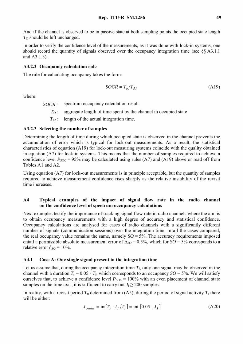
Rep. ITU-R SM.2256 49
And if the channel is observed to be in passive state at both sampling points the occupied state length TO should be left unchanged.
In order to verify the confidence level of the measurements, as it was done with lock-in systems, one should record the quantity of signals observed over the occupancy integration time (see §§ A3.1.1 and A3.1.3).
A3.2.2 Occupancy calculation rule
The rule for calculating occupancy takes the form:
AIo TTSOCR = (A19)
where:
SOCR : spectrum occupancy calculation result
TO : aggregate length of time spent by the channel in occupied state
TAI : length of the actual integration time.
A3.2.3 Selecting the number of samples
Determining the length of time during which occupied state is observed in the channel prevents the accumulation of error which is typical for lock-out measurements. As a result, the statistical characteristics of equation (A19) for lock-out measuring systems coincide with the quality obtained in equation (A7) for lock-in systems. This means that the number of samples required to achieve a confidence level PSOC = 95% may be calculated using rules (A7) and (A19) above or read off from Tables A1 and A2.
Using equation (A7) for lock-out measurements is in principle acceptable, but the quantity of samples required to achieve measurement confidence rises sharply as the relative instability of the revisit time increases.
A4 Typical examples of the impact of signal flow rate in the radio channel on the confidence level of spectrum occupancy calculations
Next examples testify the importance of tracking signal flow rate in radio channels where the aim is to obtain occupancy measurements with a high degree of accuracy and statistical confidence. Occupancy calculations are analysed for cases of radio channels with a significantly different number of signals (communication sessions) over the integration time. In all the cases compared, the real occupancy value remains the same, namely SO = 5%. The accuracy requirements imposed entail a permissible absolute measurement error of ΔSO = 0.5%, which for SO = 5% corresponds to a relative error δSO = 10%.
A4.1 Case A: One single signal present in the integration time
Let us assume that, during the occupancy integration time TI, only one signal may be observed in the channel with a duration Ts = 0.05 · TI, which corresponds to an occupancy SO = 5%. We will satisfy ourselves that, to achieve a confidence level PSOC = 100% with an even placement of channel state samples on the time axis, it is sufficient to carry out JI ≥ 200 samples.
In reality, with a revisit period TR determined from (A5), during the period of signal activity Ts there will be either:
[ ] [ ]IIIso JTJTJ ⋅=⋅= 05.0intintmin (A20)
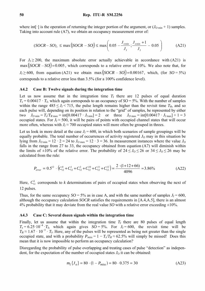
50 Rep. ITU-R SM.2256
where int[·] is the operation of returning the integer portion of the argument, or (JO min + 1) samples. Taking into account rule (A7), we obtain an occupancy measurement error of:
( )
+≤≤ 05.0–
1;–05.0max–max)–( minmin
I
o
I
or J
J
J
JSOSOCRSOSOCR (A21)
For JI ≥ 200, the maximum absolute error actually achievable in accordance with (A21) is ( ) 005.0–max =SOSOCR , which corresponds to a relative error of 10%. We also note that, for
JI ≥ 600, from equation (A21) we obtain ( ) 00167.0–max =SOSOCR , which, (for SO = 5%)
corresponds to a relative error less than 3.5% (for a 100% confidence level).
A4.2 Case B: Twelve signals during the integration time
Let us now assume that in the integration time TI there are 12 pulses of equal duration Ts = 0.00417 · TI, which again corresponds to an occupancy of SO = 5%. With the number of samples within the range 485 ≤ JI < 715, the pulse length remains higher than the revisit time TR, and so each pulse will, depending on its position in relation to the “grid” of samples, be represented by either two JO min = Ts/TR max = int[0.00417 · JI min] = 2 or three JO max = int[0.00417 · JI max] + 1 = 3 occupied states. For JI ≈ 500, it will be pairs of points with occupied channel states that will occur more often, whereas with JI ≈ 700 occupied states will more often be grouped in threes.
Let us look in more detail at the case JI = 600, in which both scenarios of sample groupings will be equally probable. The total number of occurrences of activity registered JO may in this situation be lying from JO min = 12 · 2 = 24 to JO max = 12 · 3 = 36. In measurement instances where the value JO
falls in the range from 27 to 33, the occupancy obtained from equation (A7) will diminish within the limits of ±10% of the relative error. The probability of 24 ≤ JO ≤ 26 or 34 ≤ JO ≤ 26 may be calculated from the rule:
( ) %86.34096
)66121(25.0 12
121112
1012
212
112
012
12 ≈++⋅=+++++⋅= CCCCCCPerror (A22)
Here, corresponds to k determinations of pairs of occupied states when observing the next of
12 pulses.
Thus, for the same occupancy SO = 5% as in case A, and with the same number of samples JI = 600, although the occupancy calculation SOCR satisfies the requirements in [A.4,A.5], there is an almost 4% probability that it may deviate from the real value SO with a relative error exceeding ±10%.
A4.3 Case C: Several dozen signals within the integration time
Finally, let us assume that within the integration time TI there are 80 pulses of equal length Ts = 6.25·10−4 ·TI, which again gives SO = 5%. For JI = 600, the revisit time will be TR ≈ 1.67 · 10−3 · TI. Here, any of the pulses will be represented as being not greater than the single occupied state, and with a probability Pmiss = 1 − Ts/TR ≈ 62.5% will simply be missed! Does this mean that it is now impossible to perform an occupancy calculation?
Disregarding the probability of pulse overlapping and treating cases of pulse “detection” as indepen-dent, for the expectation of the number of occupied states JO it can be obtained:
{ } ( ) 30375.080–1801 =⋅=⋅= misso PJm (A23)
12kC

Rep. ITU-R SM.2256 51
And, hence:
{ } 05.0600/301 ==SOCRm (A24)
In this way, the average occupancy value remains unbiased. This is explained by the fact that, even though some of the pulses may actually be missed, the remainder will in essence be accounted for not as being of length Ts but as lasting for a duration TR, which compensates for the previous effect.
For analysing the quality of occupancy calculations under new conditions, we shall take it that the results corresponding to a relative error within ±10% will be obtained only for a number of detected signals lying within the range from 27 to 33. The real number of detected signals will be a random value following a binomial distribution.
Taking into account, however, that with a sufficiently large overall number of detected pulses n = 80 this distribution may be approximated to normal, we obtain the following expression for the confidence level of the measurement:
%52)7.0(––)7.0(33.4
30–27–
33.4
30–33 ≈≈
= ststststSOC FFFFP (A25)
where )( zFst is a function of the probability distribution of the standard normal random value:
dtt
zFz
st
⋅
π=
∞ 2–exp
2
1)(
2
–
(A26)
and 33.4625.0375.080)–1( ≈⋅⋅=⋅⋅=σ missmiss PPn is the standard deviation of the
measurement SOCR.
Thus, with a large number of short pulses within the integration time, the occupancy values obtained will on average be close to the real values, but the confidence level of the measurement will be low (in this case PSOC = 52%).
The above examples show that for radio channels containing lengthy signals, the confidence level of the occupancy measurement depends primarily not on the occupancy value itself, but on the number of changes of state taking place in the channel in question during the integration time. Where there are infrequent changes of state in the radio channel, even a small number of samples will ensure a relatively accurate and reliable occupancy measurement. Where there are frequent changes of state in the radio channel, accurate and reliable occupancy measurement can be ensured only by significantly increasing the number of samples within the integration time.
Reference to Annex A
[А.1] Measurement procedure qualification certificate No. 206/000265/2011 on “Measurement of radio-electronic equipment emission properties with ARGAMAK-I, ARGAMAK-IM and ARGAMAK-IS Digital Measuring Radio Receivers”, including those with ARC-KNV4 Remote Controlled Frequency Down-Converter. http://www.ircos.ru/en/news.html.
[А.2] SPAULDING, A.D., HAGN, G.H. [August 1977] − On the definition and estimation of spectrum occupancy. IEEE Trans. In EMC, Vol. EMC-19, No. 3, p. 269-280.

52 Rep. ITU-R SM.2256
[A.3] KOZMIN, V.A., TOKAREV, A.B. − A method of estimating the occupancy of the frequency spectrum of an automated radio-control server in the following paginated issue of Measurement Techniques: Volume 52, Issue 12 (2009), Page 1336. http://www.springerlink.com/openurl.asp?genre=article&id=doi:10.1007/s11018-010-9442-9.
[А.4] Handbook on Spectrum Monitoring, ITU, 2011.
[А.5] Recommendation ITU-R SM.1880 − Spectrum occupancy measurement.