spectrum sensing in cognitive radio networks · 2012-11-02 · spectrum sensing in cognitive radio...
TRANSCRIPT

Spectrum Sensing in Cognitive Radio Networks
by
Sepideh Zarrin
A thesis submitted in conformity with the requirementsfor the degree of Doctor of Philosophy
Graduate Department of Electrical and Computer EngineeringUniversity of Toronto
Copyright c© 2011 by Sepideh Zarrin
Abstract
Spectrum Sensing in Cognitive Radio Networks
Sepideh Zarrin
Doctor of Philosophy
Graduate Department of Electrical and Computer Engineering
University of Toronto
2011
This thesis investigates different aspects of spectrum sensing in cognitive radio (CR) tech-
nology. First a probabilistic inference approach is presented which models the decision
fusion in cooperative sensing as a probabilistic inference problem on a factor graph. This
approach allows for modeling and accommodating the uncertainties and correlations in
the cooperative sensing system.
A constraint in the cognitive radios is the lack of knowledge about the primary signal
and channel gain statistics at the secondary users. Therefore, a practical composite
hypothesis approach is proposed which does not require any prior knowledge or estimates
of these unknown parameters.
Detection delay is an important performance measure in spectrum sensing. Quickest
detection aiming to minimize detection delay has been studied in other contexts, and we
apply it here to spectrum sensing. To combat the destructive channel conditions such as
fading, various cooperative schemes based on the cumulative sum (CUSUM) algorithm
are considered in this thesis. Furthermore, cooperative quickest sensing with imperfectly
known parameters is investigated and a new solution is derived, which does not require
any parameter estimation or iterative algorithm.
In cognitive radios, there is a fundamental trade-off between the achievable through-
put by the CRs and the level of protection for the primary user. In this thesis, this
trade-off is formulated for the quickest sensing-based CRs. By throughput analysis, it
ii

is shown that for the same protection level to the primary user, the quickest sensing
approach results in significantly higher average throughput compared to that of the con-
ventional block sensing approach.
iii

Acknowledgements
First and foremost, I would like to express my sincerest gratitude to my supervisor
Professor Teng Joon Lim for his invaluable and insightful guidance throughout the course
of my PhD study at the University of Toronto. I am always thankful for his support and
all I have learned from his great professional vision and scientific insight. This would not
be possible without him.
I wish to thank my thesis committee members, Professor Adve, Professor Valaee,
Professor Gulak and Professor Blostein for their invaluable comments. I also thank
Diane B. Silva for her the administrative support and kindness through the course my
PhD study.
I would not have been here today if it were not for the love and support of my family.
I want to express my deepest thanks to my parents for their unconditional love, devotion
and support. And my most special thanks to my husband, Saeed, for his love, support,
patience, and encouragement through my academic experience and above all, for always
being by my side through this journey of my life.
iv

Contents
List of Symbols ix
1 Introduction and Background 1
1.1 Introduction . . . . . . . . . . . . . . . . . . . . . . . . . . . . . . . . . . 1
1.2 Spectrum Sensing . . . . . . . . . . . . . . . . . . . . . . . . . . . . . . . 2
1.2.1 Matched Filtering . . . . . . . . . . . . . . . . . . . . . . . . . . . 3
1.2.2 Cyclostationary Feature Detection . . . . . . . . . . . . . . . . . . 3
1.2.3 Likelihood Ratio Test (LRT) . . . . . . . . . . . . . . . . . . . . . 4
1.2.4 Energy Detection . . . . . . . . . . . . . . . . . . . . . . . . . . . 4
1.3 Cooperative Spectrum Sensing . . . . . . . . . . . . . . . . . . . . . . . . 6
1.4 Spectrum Sensing with Unknown Parameters . . . . . . . . . . . . . . . . 7
1.5 Quickest Sensing . . . . . . . . . . . . . . . . . . . . . . . . . . . . . . . 8
1.5.1 Cooperative Quickest Sensing . . . . . . . . . . . . . . . . . . . . 9
1.5.2 Quickest Sensing with Unknown Parameters . . . . . . . . . . . . 10
1.6 Throughput of Cognitive Radio Networks . . . . . . . . . . . . . . . . . . 11
1.7 Example Application: Femtocells . . . . . . . . . . . . . . . . . . . . . . 12
1.8 Thesis Organization and Contributions . . . . . . . . . . . . . . . . . . . 14
2 Probabilistic Inference for Cooperative Sensing 17
2.1 Introduction . . . . . . . . . . . . . . . . . . . . . . . . . . . . . . . . . . 17
2.2 Model and Notation . . . . . . . . . . . . . . . . . . . . . . . . . . . . . 19
v

2.2.1 System Model . . . . . . . . . . . . . . . . . . . . . . . . . . . . . 19
2.2.2 Notation . . . . . . . . . . . . . . . . . . . . . . . . . . . . . . . . 21
2.3 Relating Probabilistic Inference to Cooperative Spectrum Sensing . . . . 21
2.3.1 Neyman-Pearson and Bayesian Methods . . . . . . . . . . . . . . 21
2.3.2 Probabilistic Inference On a Factor Graph . . . . . . . . . . . . . 23
2.3.3 Belief Propagation for Cooperative Spectrum Sensing . . . . . . . 25
2.4 NP-based LRT at the FC . . . . . . . . . . . . . . . . . . . . . . . . . . . 27
2.4.1 Hard Local Decisions . . . . . . . . . . . . . . . . . . . . . . . . . 28
2.4.2 Soft Local Decisions . . . . . . . . . . . . . . . . . . . . . . . . . 30
2.4.3 Quantized Soft Local Decisions . . . . . . . . . . . . . . . . . . . 32
2.5 Simulation Results . . . . . . . . . . . . . . . . . . . . . . . . . . . . . . 33
2.6 Chapter Summary . . . . . . . . . . . . . . . . . . . . . . . . . . . . . . 38
3 Cooperative Sensing with Unknown Parameters 40
3.1 Introduction . . . . . . . . . . . . . . . . . . . . . . . . . . . . . . . . . . 40
3.2 Model and Formulation . . . . . . . . . . . . . . . . . . . . . . . . . . . . 42
3.2.1 System Model . . . . . . . . . . . . . . . . . . . . . . . . . . . . . 42
3.2.2 NP-Based LRT at the Fusion Center . . . . . . . . . . . . . . . . 43
3.3 The Proposed Composite Hypothesis Testing Approach . . . . . . . . . . 43
3.4 The Proposed Test for Cooperative Spectrum Sensing . . . . . . . . . . . 47
3.4.1 Unknown Primary Signal and Channel Statistics . . . . . . . . . . 47
3.4.2 Unknown Primary Signal Statistics and Known Channel Statistics 51
3.4.3 Threshold Setting at the Fusion Center . . . . . . . . . . . . . . . 53
3.5 Simulation Results . . . . . . . . . . . . . . . . . . . . . . . . . . . . . . 56
3.6 Chapter Summary . . . . . . . . . . . . . . . . . . . . . . . . . . . . . . 62
4 Cooperative Quickest Sensing with Unknown Parameters 64
4.1 System Model . . . . . . . . . . . . . . . . . . . . . . . . . . . . . . . . . 67
vi

4.2 Cooperative CUSUM with Full Knowledge of Parameters . . . . . . . . . 68
4.2.1 Global CUSUM . . . . . . . . . . . . . . . . . . . . . . . . . . . . 69
4.2.2 Global CUSUM with Quantized Local Decision . . . . . . . . . . 69
4.2.3 Hard Fusion of Local CUSUM . . . . . . . . . . . . . . . . . . . . 71
4.3 Cooperative CUSUM with Unknown Parameters . . . . . . . . . . . . . . 72
4.3.1 The GLRT for Quickest Detection . . . . . . . . . . . . . . . . . . 72
4.3.2 The Rao Test for Quickest Detection Schemes . . . . . . . . . . . 72
4.3.3 The Proposed Linear Test for Quickest Detection Schemes . . . . 73
4.4 Performance Analysis and Threshold Setting . . . . . . . . . . . . . . . . 75
4.4.1 Threshold Setting for LRT-based CUSUM algorithms . . . . . . . 77
4.4.2 Threshold Setting for Linear-based CUSUM Algorithms . . . . . . 78
4.5 Simulation Results . . . . . . . . . . . . . . . . . . . . . . . . . . . . . . 79
4.6 Chapter Summary . . . . . . . . . . . . . . . . . . . . . . . . . . . . . . 84
5 Throughput of Cognitive Radio Networks 85
5.1 System Model and Problem Formulation . . . . . . . . . . . . . . . . . . 87
5.1.1 System Description . . . . . . . . . . . . . . . . . . . . . . . . . . 87
5.1.2 Problem Formulation . . . . . . . . . . . . . . . . . . . . . . . . . 88
5.1.3 CUSUM algorithm . . . . . . . . . . . . . . . . . . . . . . . . . . 89
5.2 Derivation of R(T0), Pc and IR . . . . . . . . . . . . . . . . . . . . . . . . 91
5.2.1 Quickest Spectrum Sensing . . . . . . . . . . . . . . . . . . . . . . 91
5.2.2 Block-Based Sensing . . . . . . . . . . . . . . . . . . . . . . . . . 96
5.3 Solving the Optimization Problem . . . . . . . . . . . . . . . . . . . . . . 99
5.3.1 Quickest Sensing . . . . . . . . . . . . . . . . . . . . . . . . . . . 99
5.3.2 Block-Based Sensing . . . . . . . . . . . . . . . . . . . . . . . . . 101
5.4 Simulation Results . . . . . . . . . . . . . . . . . . . . . . . . . . . . . . 102
5.5 Chapter Summary . . . . . . . . . . . . . . . . . . . . . . . . . . . . . . 107
vii

6 Conclusion 108
6.1 Summary of Conclusions . . . . . . . . . . . . . . . . . . . . . . . . . . . 108
6.2 Future Work . . . . . . . . . . . . . . . . . . . . . . . . . . . . . . . . . . 110
Bibliography 112
A Asymptotically equivalent tests for GLRT 121
A.0.1 The Wald test . . . . . . . . . . . . . . . . . . . . . . . . . . . . . 121
A.0.2 The Rao test . . . . . . . . . . . . . . . . . . . . . . . . . . . . . 121
B Derivation of the Likelihood Function 123
C Conditional distributions 125
C.1 Deriving the expected value in (5.13) . . . . . . . . . . . . . . . . . . . . 125
C.2 Deriving the expected value in (5.14) . . . . . . . . . . . . . . . . . . . . 126
C.3 Deriving the expected value in (5.15) . . . . . . . . . . . . . . . . . . . . 126
viii

List of Symbols
Symbol Description
H0 Null hypothesis
H1 Alternative hypothesis
z Primary signal
xk Observed signal at the k-th secondary user
hk Channel gain at the k-th secondary user
nk Additive noise at the k-th secondary user
uk Observation summary signal at the k-th secondary user
yk Signal received at the fusion center from the k-th secondary user
wk Channel noise from the k-th secondary user to the fusion center
αk Crossover probability of the k-th binary symmetric channel
τk Local threshold at the k-th secondary user
K The number of secondary users
N The number of sensing samples
A The maximum transmit voltage
M Modulation order
β Vector of unknown parameters
T0 The cognitive radio frame duration
T Sensing time
S Collision time
ix

List of Tables
1.1 Summary comparison of spectrum sensing schemes. . . . . . . . . . . . . 5
4.1 Average detection delay in samples for various cooperative quickest sensing
schemes. . . . . . . . . . . . . . . . . . . . . . . . . . . . . . . . . . . . . 82
x

List of Figures
1.1 Spectrum utilization measurements [1]. . . . . . . . . . . . . . . . . . . . 2
1.2 Femtocell network architecture [2]. . . . . . . . . . . . . . . . . . . . . . 13
2.1 Block diagram of complete system with K secondary users and one primary
user. The final decision made by the fusion center is denoted by θ̂. . . . . 20
2.2 Partial factor graph depicting the joint distribution (2.9). . . . . . . . . . 24
2.3 Complementary ROC (Pm vs. Pf) under AWGN SU-FC channels with
σ2n = 1, N = 200 sensing samples, σ2
h = 2 and σ2n = 8. . . . . . . . . . . . 33
2.4 Complementary ROC (Pm vs. Pf) under binary symmetric SU-FC chan-
nels with α = 0.1, N = 500 sensing samples, K = 6 secondary users,
σ2h = 2 and σ2
n = 8. . . . . . . . . . . . . . . . . . . . . . . . . . . . . . . 34
2.5 Complementary ROC (Pm vs. Pf) under binary symmetric SU-FC chan-
nels with N = 500 sensing samples, K = 6 secondary users, σ2h
K
1 = σ2n
K
1 ,
σ2n
K
1 = {1.28, 0.32, 4.5, 0.5, 2, 0.08} and αK1 = {0.2, 0.3, 0.1, 0.05, 0.2, 0.4}. . 35
2.6 Complementary ROC (Pm vs. Pf ) under soft local decisions, with N = 100
sensing samples, K = 6 secondary users, σ2n = 1, σ2
h = 2 and σ2n = 4. . . . 36
2.7 Complementary ROC (Pm vs. Pf) under quantized local decisions, with
N = 500 sensing samples, K = 6 secondary users, σ2h
K
1 = σ2n
K
1 , σ2n
K
1 =
{1.28, 0.32, 4.5, 0.5, 2, 0.08}, and αK1 = {0.1, 0.3, 0.2, 0.05, 0.1, 0.2}. . . . . 37
xi

3.1 Block diagram of cooperative spectrum sensing system with K secondary
users. . . . . . . . . . . . . . . . . . . . . . . . . . . . . . . . . . . . . . . 42
3.2 Complementary ROC (Pm vs. Pf ) curves for hard local decisions with
unknown primary statistics and K = 3. . . . . . . . . . . . . . . . . . . . 57
3.3 Complementary ROC (Pm vs. Pf ) curves for hard local decisions with
unknown primary statistics and K = 3. . . . . . . . . . . . . . . . . . . . 58
3.4 Complementary ROC (Pm vs. Pf ) curves for hard local decisions with
unknown primary statistics and K = 6. . . . . . . . . . . . . . . . . . . . 59
3.5 Complementary ROC (Pm vs. Pf) curves for soft local decisions and K =
6. . . . . . . . . . . . . . . . . . . . . . . . . . . . . . . . . . . . . . . . 60
3.6 Complementary ROC (Pm vs. Pf ) curves for 2-bit quantized local decisions
with unknown primary statistics. . . . . . . . . . . . . . . . . . . . . . . 61
3.7 Complementary ROC (Pm vs. Pf ) curves for 2-bit quantized local decisions
with unknown primary and channel gain statistics. . . . . . . . . . . . . 62
3.8 Probability distribution function of the linear test statistic under the null
hypothesis. . . . . . . . . . . . . . . . . . . . . . . . . . . . . . . . . . . . 63
4.1 Probability of false alarm, Pf , versus average detection delay Td. . . . . . 79
4.2 Probability of false alarm, Pf , versus average detection delay Td. . . . . 80
4.3 Probability of false alarm, Pf , versus threshold q. . . . . . . . . . . . . . 83
5.1 A CR frame, showing the sensing interval in black and the data transmis-
sion phase in a lighter shade. The primary user is inactive at the start
of the frame (defined as event H0 in the text), and comes on at time
T + X from the start of the frame, leading to collision over a duration
S = T0 − T − X. . . . . . . . . . . . . . . . . . . . . . . . . . . . . . . . 88
5.2 Average normalized throughput, RQ/C0, and probability of collision, PcQ,
versus frame duration T0 for quickest sensing. . . . . . . . . . . . . . . . 103
xii

5.3 Average normalized throughput, RQ/C0, and primary interference time
ratio (PITR), IRQ, versus frame duration T0 for quickest sensing. . . . . . 104
5.4 Average normalized CR throughput, versus probability of collision. . . . 105
5.5 Average normalized CR throughput, versus probability of collision. . . . 106
xiii

Chapter 1
Introduction and Background
1.1 Introduction
Studies have shown that most of the licensed radio-wave spectral bands are under-utilized
in time and space domain [1,3,4], resulting in unused “white spaces” in the time-frequency
grid at any particular location. The spectrum utilization is mainly around certain parts of
the spectrum whereas a considerable amount of the spectrum is unutilized as depicted in
Figure 1.1. As can be observed, spectrum utilization is more intense and competitive at
frequencies below 3 GHz whereas the spectrum is under-utilized in the 3-6 GHz bands [1].
The Federal Communications Commission (FCC) has also reported the temporal and
geographic variations in spectrum utilization to range from 15% to 85% [3]. On the
other hand, fixed spectrum allocation policies do not allow for reusing of the rarely used
spectrum allocated to licensed users by unlicensed users. This problem coupled with the
rapidly increasing demand for wireless services and radio spectrum has led to spectrum
scarcity for wireless applications.
This has necessitated a new communication standard that allows unlicensed (sec-
ondary) users to utilize the vacant bands which are allocated to licensed (primary) users.
However, this opportunistic access should be in a manner that does not interrupt any
1

Chapter 1. Introduction and Background 2
Figure 1.1: Spectrum utilization measurements [1].
primary process in the band. Therefore, the secondary users must be aware of the activ-
ity of the primary user in the target band. They should spot the spectrum holes and the
idle state of the primary users in order to exploit the free bands and also promptly vacate
the band as soon as the primary user becomes active. Cognitive radio, encompasses this
awareness by dynamically interacting with the environment and altering the operating
parameters with the mission of exploiting the unused spectrum without interfering with
the primary users [5, 6]. Showing support for the cognitive radio idea, the FCC allowed
for usage of the unused television spectrum by unlicensed users wherever the spectrum is
free [6,7]. IEEE has also supported the cognitive radio paradigm by developing the IEEE
802.22 standard for wireless regional area network (WRAN) which works in unused TV
channels [8].
1.2 Spectrum Sensing
In order to maintain the primary users’ right to interference-free operation, the secondary
users need to regularly sense the allocated band and reliably detect the presence of the

Chapter 1. Introduction and Background 3
primary users’ signals with little delay. In the IEEE 802.22 standard, for example, the
secondary users need to detect the TV and wireless microphone signals and upon their
detection, they are required to vacate the channel within two seconds [8]. For TV primary
signals, a probability of detection of 90% and a probability of false alarm of 10% should
be maintained [8]. Therefore, spectrum sensing plays a crucial role in the cognitive radio
technology to prevent damaging interference to the primary users and to reliably and
quickly spot the white spaces in the spectrum and utilize the opportunity.
Various spectrum sensing methods are used in literature depending on how much
information about the primary signal is available to the secondary users, as discussed in
the following.
1.2.1 Matched Filtering
Matched filtering-based methods are optimal for stationary Gaussian noise scenarios as
they maximize the received SNR [9, 10]. For this optimal performance, they require
perfect knowledge of the channel responses from the primary user to the secondary user
and the structure and waveforms of the primary signal (including modulation type, frame
format and pulse shape) as well as accurate synchronization at the secondary user [9–12].
In cognitive radios, however, such knowledge is not readily available to secondary users
and implementation cost and complexity of this detector is high especially as the number
of primary bands increases. Therefore, this method is not practical and applicable to
cognitive radio technology.
1.2.2 Cyclostationary Feature Detection
Another detection method that can be applied for spectrum sensing is the cyclostationary
feature detector. Cyclostationary feature detectors can distinguish between modulated
signals and noise [9–14]. This detector exploits the fact that the primary modulated
signals are cyclostationary with spectral correlation due to the built-in redundancy of

Chapter 1. Introduction and Background 4
signal periodicity (e.g., sine wave carriers, pulse trains, and cyclic prefixes), while the
noise is a wide-sense stationary signal with no correlation [13, 14]. This task can be
performed by analyzing a spectral correlation function. Therefore, cyclostationary feature
detectors are robust to the uncertainty in noise power [9–14]. This is at the price of
excessive computational complexity and long observation times. Moreover, it requires
the knowledge of the cyclic frequencies of the primary users, which may not be available
to the secondary users.
1.2.3 Likelihood Ratio Test (LRT)
Spectrum sensing is a binary hypothesis testing problem, with the null and alternative
hypotheses
H0 : Primary user not active
H1 : Primary user active(1.1)
Based on the Neyman-Pearson (NP) theorem [15], the test statistic that maximizes the
probability of detection for a given probability of false alarm is the likelihood ratio test
(LRT) defined as
L(X) =p(X|H1)
p(X|H0)(1.2)
where X denotes the received signal vector and p(·) denotes the probability density
function (PDF).
The LRT, which is proven to be NP optimal [15], requires the exact distributions of
primary signal and noise and channel gains which makes it practically intractable.
1.2.4 Energy Detection
For a Gaussian noise model, when the noise power is known to the secondary user energy
detection can be applied to detect the existence of the primary signal. This simple scheme
accumulates the energy of the received signal during the sensing interval and declares
the band to be occupied if the energy surpasses a certain threshold. This threshold is set

Chapter 1. Introduction and Background 5
Spectrum Sensing Scheme Advantages Disadvantages
Matched Filtering Optimum performance Requires full primary signal
knowledge, high power con-
sumption and implementa-
tion complexity
Cyclo Feature Detection Robust to interference and
noise uncertainty
High computational com-
plexity, vulnerable to
sampling clock offsets and
model uncertainties, long
observation time
LRT detection NP-optimal performance Requires exact distributions
and parameters
Energy Detection Low complexity, no primary
knowledge required
Vulnerable to noise uncer-
tainty
Table 1.1: Summary comparison of spectrum sensing schemes.
Chapter 1. Introduction and Background 6
based on the desired probability of false alarm [15,16]. Energy detection, unlike the other
schemes, does not require any information about the primary signal and channel gains
and is robust to unknown fading channel. Compared to other methods it has simpler
implementation and hence is less expensive. Therefore, in literature energy detection is
mainly adopted for spectrum sensing [9–12,17–20].
Table 1.1 presents a brief comparison of the above spectrum sensing schemes.
1.3 Cooperative Spectrum Sensing
In practice, the reliability of spectrum sensing in detecting weak primary signals is
hard to maintain due to the destructive channel conditions such as multi-path fad-
ing or shadowing between the primary user and the secondary users. As different
users in distant locations undergo independent fading channels, allowing cooperation
among them can improve the overall detection reliability by utilizing the inherent di-
versity [9, 10, 17–19, 21–24]. In this manner, the individual secondary users require less
detection sensitivity whereas the overall detection reliability is improved. This means
having more accurate and agile detection, fewer false alarms and more protection to the
primary user [12, 20, 23–25]. The problem of hidden terminals can also be alleviated
through cooperation among fairly distant secondary users [12, 20, 23, 25]. These advan-
tages come at the price of added communication overhead due to cooperation. The FCC
has also acknowledged the need for cooperative spectrum sensing for TV bands [26, 27].
In a widely studied form of cooperative spectrum sensing, the secondary users provide
locally-sensed information on the primary user’s activity status to a decision-making
fusion center (FC) which can be an access point or base station or another secondary
user [9,10,17–19,21–24]. The fusion center analyzes the information and determines the
activity status of the primary user.
The cooperative sensing schemes can be mainly categorized based on the type of fusion

Chapter 1. Introduction and Background 7
method used at the fusion center. Hard-decision combining schemes such as AND/OR
and M-out-of-K rules are considered in [17,18] where their performances are compared.
It is shown that when one node has much higher SNR compared to other nodes then
cooperative spectrum sensing performs worse than the single node spectrum sensing.
Soft decision combining rules such as linear combination of local energies [19, 22] and
LRT approach [17, 21] are also considered in the literature. In LRT-based schemes, the
local decision statistics are either assumed to be available [17], or estimated [21] at the
fusion center. The summation of the secondary users’ received signal energies has been
considered as a soft decision based cooperative sensing method in [19]. A cooperative
sensing scheme based on linear combination of the local test statistics was proposed in [22]
where the combining weights were optimized to improve the detection performance.
In the above studies, the SU-FC channels were assumed to be error- or noise-free.
There was also no mention of how to make use of knowledge about the modulation
format used at the primary transmitter, or correlations in time or space of the channels
linking the primary transmitter to the secondary users. For a more rigorous study, we
propose a probabilistic inference approach for cooperative spectrum sensing in Chapter
2.
1.4 Spectrum Sensing with Unknown Parameters
An important constraint in cognitive radios is the lack of knowledge about the primary
signal and channel statistics at the secondary users and the fusion center. Therefore the
LRT-based methods which perform better than other approaches cannot be applied in
cognitive radios due to unknown parameters and uncertainties in likelihood functions.
These unknown parameters in cognitive radios, which are mainly the statistics of the
primary signal and channel gains, appear in the likelihood function under H1. We denote
them here by β. In detection theory, hypothesis testing in the presence of uncertain
Chapter 1. Introduction and Background 8
parameters is known as composite hypothesis testing [15]. The main approach to tackle
this problem is the generalized likelihood ratio test (GLRT) [15]. This test first finds the
maximum likelihood estimate (MLE) of the unknown parameters under H1, and then
forms the GLRT statistic:
LG(X) =p(X|β = β̂,H1)
p(X|H0)(1.3)
where β̂ = arg maxβ p(X|β,H1) and β = 0 under H0.
An asymptotically (as the number of observations increase) equivalent test for GLRT
is the Wald test with statistic
TW (X) = β̂TI(β̂)β̂, (1.4)
where I(·) is the Fisher information matrix (see [28] pg. 40). The Wald test requires the
derivation of the MLEs. However, the analytical derivation of the MLEs is complicated
and even intractable for a general cooperative noisy channel model.
Another asymptotic equivalent test for GLRT is the Rao test which does not require
the MLE of the unknown parameters and is simpler computationally [15]. The Rao test
statistic is given by
TR(X) =∂ ln p(X|β)
∂β
∣
∣
∣
T
β=0I−1(0)
∂ ln p(X|β)
∂β
∣
∣
∣
β=0(1.5)
The Rao test, in fact, is not practical as the Fisher information matrix is not easily attain-
able or invertible in many system models. Dealing with multiple unknown parameters
in cooperative spectrum sensing, even further adds to the complexity and infeasibility of
calculating this inverse matrix. In Chapter 3, we propose a practical composite hypoth-
esis testing approach which estimates the unknown parameters, and further simplify it
so that it does not even require these estimates.
1.5 Quickest Sensing
The cooperative spectrum sensing approaches that we discussed so far had a classic
detection framework, in which the goal is to minimize the miss-detection probability

Chapter 1. Introduction and Background 9
subject to constraints on the false alarm probability. Their detection approach is block-
based, where the secondary users take a block of samples, and decide on the activity
state of the primary user based on these samples. However, other than the probability of
detection, detection delay is also crucial to cognitive radios in order to act quickly upon
vacancy or occupancy of the primary band. The vacancy of the primary band should be
sensed quickly so that the secondary transmission starts right away and the opportunity
is utilized efficiently. On the other hand, upon the activity of the primary user the
secondary user should be able to sense and act quickly and vacate the band promptly
in order not to disrupt the primary transmission. Therefore a detection framework is
required which allows for analysis and minimization of the detection delay for a certain
level of false alarm [29].
In essence, the spectrum sensing is detection of change in spectrum activity (emer-
gence of the primary radio and/or vacancy of the band). Therefore, we can apply the
theory of sequential change detection, which performs a statistical test to detect the
change of distribution in observations as quickly as possible, in order to attain an agile
and robust spectrum sensing [30]. The adaptation of this approach to spectrum sensing
is known as quickest sensing in literature [30–32]. In the sequential change detection lit-
erature, the well-known Page’s cumulative sum (CUSUM) algorithm [33] has been shown
to be optimal in the sense of minimizing the detection delay while maintaining an ac-
ceptable level of false alarm [34–36]. In [30–32], the CUSUM algorithm has been applied
to quickest spectrum sensing in cognitive radios.
1.5.1 Cooperative Quickest Sensing
Due to fading and path loss effects in cognitive radio networks, single user sensing is
proven to be unreliable and the detection performance improves with the number of
available sensors that make independent observations [32,37,38]. The study of distributed
quickest detection has been based on two different formulations in the detection literature.

Chapter 1. Introduction and Background 10
One is based on a Bayesian formulation in which the change point (time at which the
change occurs) is assumed to have a known prior distribution [29, 39, 40]. In this case,
the joint optimization of local users and the fusion center policies over time becomes
hard or intractable [40]. However, a tractable test design is developed for a geometric a
priori distribution for the change time in [29, 39]. The other formulation is the minimax
formulation, proposed by Lorden [34], for which Pages CUSUM procedure is the optimal
scheme. The asymptotically optimal cooperative CUSUM-based approaches for various
local memory and transmission rate scenarios have been studied by Mei [37]. We apply
and compare three CUSUM-based cooperative spectrum sensing schemes in cognitive
radios with noisy channels: global CUSUM with soft local decisions, global CUSUM
with quantized local decisions and hard fusion of local CUSUM to cognitive radios as
described in Chapter 4.
1.5.2 Quickest Sensing with Unknown Parameters
In practice, when the primary user starts transmission there are unknown parameters
in the distribution of the observed signals, e.g. the variance of the observed signals,
due to unknown primary signal statistics and channel gains between the primary and
secondary users. Therefore, the CUSUM-based approaches that are based on perfectly
known distributions cannot be directly applied to spectrum sensing in cognitive radios.
Therefore, quickest detection schemes that can accommodate unknown parameters should
be developed.
The GLRT was adopted by Lorden [34] for CUSUM with unknown parameters. How-
ever, due to the non-recursive expression of the GLRT-based CUSUM and the need to
store all the observations and re-estimate the unknown parameters in all time slots, this
algorithm turns out to be infeasible and impractical. The parallel CUSUM test [41] re-
quires a complicated recursive algorithm and does not achieve the optimal performance.
The successive refinement algorithm [31] which performs estimation while detecting em-

Chapter 1. Introduction and Background 11
beds incremental estimation in the parallel CUSUM test for the unknown parameter and
is suitable only for scenarios with unknown parameters that can be estimated incremen-
tally. Otherwise, it needs to store of all samples like the GLRT algorithm. In Chapter
4 we introduce our linear method which does not require any complicated algorithm or
parameter estimation and accommodates multiple unknown parameters.
1.6 Throughput of Cognitive Radio Networks
Associated with spectrum sensing are two parameters: probability of detection and prob-
ability of false alarm. The higher the detection probability, the better the primary users
can be protected. However, from the secondary users perspective, the lower the false
alarm probability, the more chances the channel can be reused when it is available, thus
the higher the achievable throughput for the secondary users. Thus there exists a funda-
mental tradeoff between sensing capability and achievable throughput for the secondary
network.
In block sensing schemes1, the sensing time can be chosen to achieve the desired
throughput for the CRs while satisfying the regularity constraints for primary user’s pro-
tection from interference. In [42], the optimum sensing time has been formulated under
both presence and absence of the primary signal. Upon finding an available channel, the
optimization problem is to find the optimum in-band sensing time such that the maxi-
mum average throughput is achieved. The sensing-throughput trade-off is also considered
in [43] where the CR’s average throughput is maximized for a certain level of certainty
in detecting the primary signal.
In [43], the block sensing duration was designed to maximize CR throughput with
a given frame duration, while protecting the primary user by keeping the probability
of detection higher than a certain threshold. Similar problem of optimizing the frame
1Where the sensing phase is fixed in duration.
Chapter 1. Introduction and Background 12
duration for a given sensing time has been considered in [44, 45]. In [44], the objective
of the optimization was to maximize the CR’s throughput while keeping the probability
of collision with the primary user below a certain threshold, assuming that primary user
activity in successive frames are independent of each other. In [45], the throughput of
the CR was maximized while ensuring that the primary interference time ratio (PITR)
is less than a certain threshold. Unlike [44], it assumed dependent primary signals in
successive frames by modeling the primary user activity as a continuous time Markov
process. Both [44] and [45] assume perfect error-free block sensing which is not realistic
and they neglect the effect of interference from the primary user on the CR’s throughput.
While in all of the above throughput analysis only block sensing approach is consid-
ered, in Chapter 5, we investigate the sensing-throughput tradeoff for quickest sensing-
based CR networks. We analyze the average CR throughput for both quickest and block
sensing approaches, and unlike the previous work, we consider a drop in the CR through-
put due to interference from the primary user.
1.7 Example Application: Femtocells
A practical application and supporting infrastructure for cognitive radio networks is the
femtocell network [46]. Femtocells are home base stations which improve indoor coverage
and service quality in cellular networks [2,46]. These low-power access points are installed
at homes or small public places and by improving the spectral efficiency and indoor
coverage they reduce the overall and operational costs [46]. Figure 1.2 depicts an example
femtocell network. The femtocells backhauls data to the cellular operator network or the
Internet backbone through a broadband connection such as DSL, TV cable, fiber, power
line or Ethernet [46,47]. The existing wired backhaul infrastructure makes femtocells an
ideal candidate for cognitive radio implementation by allowing cooperation among users.
Spectrum sensing can be performed by individual femtocells and the sensing results can

Chapter 1. Introduction and Background 13
Figure 1.2: Femtocell network architecture [2].
be shared by other users. By utilizing the existing infrastructure of femtocell networks
for CRs, the issues in deployment, hardware, security, and network management of CRs
can be tackled easily and cost efficiently.
In [46], the conventional femtocell concept was extended to enable cognitive operation.
The femtocell base station (FBS), provides backhauling service via a wired broadband
IP connection to the users in its coverage region. The FBS performs local sensing to find
the unused spectrum by the primary users in its region and the neighboring femtocells
and to control interference to the underlaying macrocell and nearby femtocells. The only
change required to the current handsets is a software update to support the cognitive
mode and provide application level tools and protocol modifications.
In order to improve sensing reliability and decrease interference to nearby femtocells
and underlying macrocell, cooperative sensing can be performed in femtocell networks.
As mentioned before, the existing wired backhaul in femtocells is a favorable infrastruc-
ture for cooperative spectrum sensing among femtocells. Cooperative sensing among
nearby FBSs improves the sensing reliability and increases the sensing domain. More-
over, this could alleviate interference among femtocells and between femtocells and the

Chapter 1. Introduction and Background 14
underlying macrocell which results in higher system capacity.
1.8 Thesis Organization and Contributions
In Chapter 2 of this thesis, the probabilistic approach for cooperative spectrum sensing
is presented. The main contributions of this chapter are outlined as follows.
• A probabilistic inference approach for cooperative spectrum sensing is proposed.
The cooperative sensing system is probabilistically modeled on a representative fac-
tor graph, and the decision fusion problem is approached as a probabilistic inference
problem on a factor graph that can be tackled by message passing algorithms like
belief propagation.
• The proposed approach allows for modeling and accommodating the uncertainties
and correlations in the cooperative sensing system.
• Unlike most studies in this field, nonideal transmission channels between secondary
users and fusion center as well as the presence of fading in links between primary
and secondary users are considered.
• The likelihood ratio test statistics are derived for one-bit, multi-bit or infinite pre-
cision of local decisions.
In Chapter 3, the spectrum sensing problem with unknown parameters is investigated.
The main contributions of this chapter are as follows.
• A novel composite hypothesis testing approach for spectrum sensing with unknown
parameters is proposed which does not require any prior knowledge about the
primary signal and channel statistics.
• A simple spectrum sensing scheme is proposed for cognitive radios with unknown
parameters, which does not require any parameter estimation or iterative algorithm.

Chapter 1. Introduction and Background 15
• The proposed test has been applied to cooperative spectrum sensing with hard,
soft and quantized local decisions and the corresponding test statistics are derived
under the unknown primary signal and channel statistics scenario.
• The locally most powerful (LMP) detector has been adopted for decision making at
the fusion center for weak constant-modulus primary signals and its corresponding
test statistic has been derived.
• An analytical threshold setting scheme is presented for the proposed test as well as
the LMP.
• Performance comparison between the proposed test and LRT is provided. The
results illustrate the close performance of the proposed test to the optimal LRT.
In Chapter 4, cooperative quickest spectrum sensing is investigated. The main contribu-
tions of this chapter are as follows.
• Several cooperative quickest sensing schemes based on the CUSUM algorithm are
presented for cognitive radios and their test statistics under noisy and noiseless
channel scenarios are derived.
• A linear test for cooperative spectrum sensing with unknown parameters is pre-
sented, which does not require any prior knowledge or estimation of the primary
signal or channel statistics. This test is very simple and does not entail any iterative
or complicated algorithms.
• A threshold setting method for CUSUM-based algorithms and the proposed test is
presented for a target probability of false alarm.
Chapter 5 presents the throughput analysis of cognitive radio networks. The main con-
tributions of this chapter are outlined as follows.
• The throughput-sensing tradeoff is formulated and analyzed for quickest sensing.

Chapter 1. Introduction and Background 16
• Analytical expressions for the average throughput, probability of collision and
PITR (primary interfered time ratio) for both quickest and block-based sensing
approaches are derived for the realistic assumption that collision with PUs causes
a drop in throughput for the CR.
• The optimal frame durations of quickest and block-based sensing CRs to achieve the
maximum CR throughput are found, while protecting the primary user by keeping
the collision probability or PITR below a certain threshold.
• The maximum achievable throughput with block and quickest sensing schemes are
compared and shown that for the same protection level to the primary network,
the quickest sensing approach results in significantly higher average throughput.
Finally, the thesis is concluded in Chapter 6 by presenting some final remarks and future
research directions.

Chapter 2
Probabilistic Inference Approach for
Cooperative Sensing
2.1 Introduction
Cooperative spectrum sensing has been introduced to address the problem of detection
reliability of weak primary signals under fading and hidden terminal problem condi-
tions [17–19, 21, 22]. In a widely studied form of cooperative spectrum sensing, the
secondary users provide locally-sensed information on the primary user’s activity status
to a decision-making fusion center (FC) which can be an access point or base station.
Intuitively, the resulting diversity improves detection performance by deciding based on
multiple observations of the same signal. The problem of hidden terminals can also be
alleviated by cooperation among distant secondary users from each other. Cooperative
sensing is helpful when the cooperating users are close enough together that the same
primary activity level applies to them all, but still far enough apart that the channels
are independent.
The cooperative spectrum sensing schemes studied in the literature are mostly based
on either hard-decision combining schemes such as logical AND/OR and M-out-of-K
17

Chapter 2. Probabilistic Inference for Cooperative Sensing 18
rules [17,18], or soft decision combining rules such as linear combination of local energies
[22] or LRT approaches [17, 21]. In these studies, the SU-FC channels were assumed to
be error and noise free, which is unrealistic especially for the infinite-precision energy-
combining methods, in which the FC is assumed to know the energy measured at the
secondary users precisely.
In this chapter, we propose a probabilistic inference approach for cooperative spec-
trum sensing – we probabilistically model the cooperative sensing system with a factor
graph, and approach the decision fusion or detection problem as a probabilistic inference
problem on a factor graph that can be tackled by belief propagation (BP) [48]. The
likelihood ratio test at the FC, based on Neyman-Pearson (NP) or Bayesian criteria [15],
is then straightforward to compute. This approach can accommodate the uncertainties
and correlations in cooperative sensing and provide fresh insight into statistical cooper-
ative spectrum sensing. For instance, with the proposed method we are able to consider
Rayleigh fading PU-SU channels as well as noisy SU-FC channels for added realism
compared to the existing studies in the CR literature.
Using the proposed approach, we derive the optimal NP-based LRT at the FC for
hard, soft and quantized local decisions. For the hard decision scenario, we consider
two different models for the SU-PU channels: binary symmetric channels (BSCs) and
additive white Gaussian noise (AWGN) channels. In the BSC scenario, we show that
under the same channel conditions and local thresholds for all the secondary users, the
NP-based LRT is equivalent to the M-out-of-K rule where the licensed band is declared
to be occupied if at least M out of the K secondary users have detected the primary
signal. Under the AWGN channel scenario, we show that the LRT performs better than
the M-out-of-K, AND and OR fusion rules. For the soft local decisions scenario where
the secondary users send their local test statistics to the FC, we consider AWGN SU-FC
channels and derive the LRT at the FC. We show that the LRT outperforms the adding,
maximal ratio combining and selection combining methods.

Chapter 2. Probabilistic Inference for Cooperative Sensing 19
Finally, we discuss the transmission of multi-bit quantized soft local decisions from
each secondary user to the FC. Given that the received energy is the sufficient test statistic
for Gaussian channels [49], we consider energy quantization at the secondary users and
derive the LRT at the FC using the BP approach. We show that by sending only two
bits of information on the signal energy from all the secondary users, the performance
of the NP-based LRT improves significantly compared to the case of hard (one-bit) local
decisions. The results of this chapter have been published partly in [50].
The remainder of this chapter is organized as follows. The system model and notations
are described in Section 2.2. The relation between detection and probabilistic inference
and the proposed graphical model approach are presented in Section 2.3. The derivation
of NP-based LRT at the FC for hard, soft and quantized local decisions is provided
in Section 2.4. The simulation results and performance comparisons are provided in
Section 2.5. Finally, Section 2.6 concludes the chapter.
2.2 Model and Notation
2.2.1 System Model
We consider a centrally coordinated cognitive radio network with K secondary users.
We denote the baseband-equivalent signal transmitted by the primary user over a sens-
ing interval of N samples by z, where the underscore denotes a vector of N samples
in time. This signal is propagated to the k-th secondary user over a frequency non-
selective channel that is time invariant over N sampling intervals1. The observed complex
baseband-equivalent signal at the k-th secondary user over N sampling intervals is
xk = hkz + nk (2.1)
1Here we prefer to present a simple channel model to illustrate the technique proposed. Nevertheless,time-varying channels can also be included in the model.

Chapter 2. Probabilistic Inference for Cooperative Sensing 20
where nk denotes the zero-mean additive white Gaussian noise (AWGN) i.e., nk ∼
CN (0, σ2nk
I) and hk represents the circularly symmetric complex Gaussian (CSCG) chan-
nel gain i.e. hk ∼ CN (0, σ2hk
). Moreover, z, hk and nk are assumed to be independent,
which is reasonable from a practical perspective.
The observed signal at the k-th secondary user is mapped onto an observation sum-
mary signal uk over N sampling intervals, i.e.,
uk = γk(xk) (2.2)
In this chapter, we assume three different scenarios for the local mappings at the sec-
ondary users; hard-decision cooperation, where uk is the output of energy detection at
the k-th secondary user, soft-decision cooperation where uk is the energy of xk, and
quantized-decision cooperation where uk is the quantized energy of xk.
PUz
- m×?
hK
- m+?
nK
-
xKγK(xK) -
uKp(yK |uK) -
yK
- m×?
h1
- m+?
n1
-
x1γ1(x1)
-
u1p(y1|u1) -
y1
FCDec.Dev.
-θ̂
ssss
ssss
PU → SU SU → FC
Figure 2.1: Block diagram of complete system with K secondary users and one primary
user. The final decision made by the fusion center is denoted by θ̂.
As shown in Figure 2.1, uk is subsequently transmitted to the fusion center where
the final spectrum occupancy decision is made. We assume the channel between each
secondary user and the FC to be noisy and characterized by p(yk|uk), where yk denotes the

Chapter 2. Probabilistic Inference for Cooperative Sensing 21
signal received at the FC from k-th secondary user. This characterization is general and
different models can be considered for the SU-FC channels. In this chapter, we consider
two different models for the SU-FC channels: binary symmetric channels with crossover
probabilities αks, as well as AWGN channels with additive noise wk ∼ CN (0, σ2wk
). In the
latter case, p(yk|uk) = pwk(yk − uk) = 1
πσ2wk
exp(− |yk−uk|2σ2
wk
). The evidence available to the
FC to make the global decision is the set of SU-FC channel outputs yK1 = {y1, . . . , yK}.
2.2.2 Notation
We define the following notations which are used throughout this chapter. vK1 denotes
the set {v1, . . . , vK} which can also be collected into the vector form [v1, . . . , vK ]. The
underscored variable v denotes vector of N samples in time. There is no distinction made
between random variables and their values, e.g. p(z) is the probability density function of
the random variable z, except in the factor graph in Figure 2.2 and discussions referring
to Figure 2.2, where capital letters are used to denote random variables by convention.
2.3 Relating Probabilistic Inference to Cooperative
Spectrum Sensing
2.3.1 Neyman-Pearson and Bayesian Methods
Spectrum sensing is a binary hypothesis testing problem, with the null and alternative
hypotheses
H0 : Primary user not active : z = 0,
H1 : Primary user active : z 6= 0.(2.3)
There are two well-known strategies for solving a binary hypothesis testing problem;
Baysian method and Neyman-Pearson (NP) method [15]. The Bayesian method is based
on the minimization of a Bayesian risk function which, under equal costs of a false

Chapter 2. Probabilistic Inference for Cooperative Sensing 22
alarm and missed detection, reduces to the minimization of the probability of error. By
introducing θ ∈ {0, 1} as indices to the null and alternative hypotheses, the probability
of error can be represented by P (θ̂ 6= θ), where θ̂ is the decision on θ. The NP method
is based on the maximization of the probability of detection P (θ̂ = 1|θ = 1), while
maintaining a given probability of false alarm P (θ̂ = 1|θ = 0).
The optimal decision that minimizes the probability of error is the maximum a pos-
teriori (MAP) decision [15]
θ̂ = arg maxθ∈{0,1}
P (Hθ|yK1 ). (2.4)
If no prior information on Hθ is available, the MAP decision is equivalent to the maximum
likelihood (ML) decision which is equivalent to choosing H1 if and only if
p(yK1 |z 6= 0)
p(yK1 |z = 0)
>1
2. (2.5)
The optimal NP method similarly employs a likelihood ratio test (LRT) [15] by choos-
ing H1 if and only if
L(yK1 ) =
p(yK1 |z 6= 0)
p(yK1 |z = 0)
> λ, (2.6)
where the threshold λ is found by solving (numerically or analytically)
Pf =
∫
yK1 :L(yK
1 )>λ
p(yK1 |z = 0)dyK
1 (2.7)
for a given desired probability of false alarm Pf .
In both (2.5) and (2.6), we need to evaluate the likelihood function p(yK1 |z) for z = 0
and otherwise. From Bayes’ rule, we have
p(yK1 |z) ∝ p(z|yK
1 )
p(z)(2.8)
or in other words, the likelihood can be found from the a posteriori probability (APP)
distribution of z. The detection problem can therefore be decomposed into a Bayesian
inference problem, namely finding P (z = 0|yK1 ) and P (z 6= 0|yK
1 ).

Chapter 2. Probabilistic Inference for Cooperative Sensing 23
2.3.2 Probabilistic Inference On a Factor Graph
As discussed above, the cooperative spectrum sensing problem can be reduced to finding
the APP for null and alternative hypotheses. The APP p(z|yK1 ) can be obtained by
marginalizing over all other random variables in the model. For the model presented in
Section 2.2, the joint distribution is
p(z, uK1 , xK
1 , hK1 |yK
1 ), (2.9)
and the required APP is
p(z|yK1 ) =
∫
p(z, uK1 , xK
1 , hK1 |yK
1 )duK1 dxK
1 dhK1 . (2.10)
For factorizable joint probability distributions, with each factor being a function of
only a small subset of the total set of variables, marginalization may be efficiently per-
formed using the so-called belief propagation2 with the aid of a factor graph [48]. A
factor graph is a bipartite graph that represents the factorization of a function. A factor
graph consists of variable nodes, factor nodes and edges. For a certain factorization of a
function, the edges connect the factor nodes to the variable nodes that they are a func-
tion of [51]. BP obtains exact results for loop-free or tree graphs, and when the graph
is “locally” tree-like but not actually a tree, very accurate results arise in iterative BP.
In the following, we will demonstrate that the factor graph for (2.9) is, in fact, a tree
(if channel coefficients hj and hk are independent for j 6= k). Thus, BP can be used to
obtain a cooperative sensing algorithm that is based on firm probabilistic foundations.
From the conditional probability chain rule, we have
p(z, uK1 , xK
1 , hK1 |yK
1 ) = p(uK1 |yK
1 )p(xK1 |uK
1 , yK1 )p(hK
1 , z|xK1 , uK
1 , yK1 )
2also known as message passing, and the sum-product algorithm
Chapter 2. Probabilistic Inference for Cooperative Sensing 24
p(yk−1|uk−1) p(yk|uk)
Uk−1UkXk−1 Xk
p(hk−1) p(hk)
p(xk−1|z, hk−1) p(xk|z, hk)
I(uk−1 = γk−1(xk−1)) I(uk = γk(xk))
Hk−1 Hk
p(z)
Z
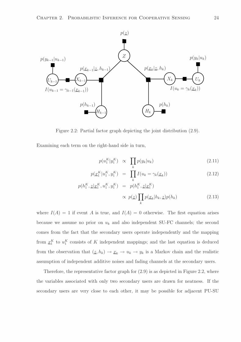
Figure 2.2: Partial factor graph depicting the joint distribution (2.9).
Examining each term on the right-hand side in turn,
p(uK1 |yK
1 ) ∝∏
k
p(yk|uk) (2.11)
p(xK1 |uK
1 , yK1 ) =
∏
k
I(uk = γk(xk)) (2.12)
p(hK1 , z|xK
1 , uK1 , yK
1 ) = p(hK1 , z|xK
1 )
∝ p(z)∏
k
p(xk|hk, z)p(hk) (2.13)
where I(A) = 1 if event A is true, and I(A) = 0 otherwise. The first equation arises
because we assume no prior on uk and also independent SU-FC channels; the second
comes from the fact that the secondary users operate independently and the mapping
from xK1 to uK
1 consists of K independent mappings; and the last equation is deduced
from the observation that (z, hk) → xk → uk → yk is a Markov chain and the realistic
assumption of independent additive noises and fading channels at the secondary users.
Therefore, the representative factor graph for (2.9) is as depicted in Figure 2.2, where
the variables associated with only two secondary users are drawn for neatness. If the
secondary users are very close to each other, it may be possible for adjacent PU-SU
Chapter 2. Probabilistic Inference for Cooperative Sensing 25
channels, Hk and Hk−1, to be correlated. This would be depicted in the factor graph
with a connection between Hk and Hk−1, represented by the factor node p(hk|hk−1).
Alternatively, it may be more realistic to assume that all Hks are independent, which
would simplify the graph and the resulting message passing algorithm. The factor graph
can also be easily modified to model correlations in time, for instance expressed in a
Markov chain for each Hk.
Finally, if uk is dependent only on a function of xk, e.g. its energy ‖xk‖2, the variable
node xk in the factor graph may be replaced by that function, say tk. In other words,
I(uk = γk(xk)) → I(uk = Γk(tk)) and p(xK1 |hK
1 , z) → p(tK1 |hK1 , z), where tk = ‖xk‖2, and
Γk(‖xk‖2) = γk(xk). The joint distribution of interest is now
p(z, uK1 , tK1 , hK
1 |yK1 ) ∝ p(z)
K∏
k=1
p(yk|uk)I(uk = Γk(tk))p(tk|hk, z)p(hk). (2.14)
In this chapter, we assume that energy detection is used by each secondary user, and
make use of the above transformation in the next section.
2.3.3 Belief Propagation for Cooperative Spectrum Sensing
Having identified the factor graph characterizing the cooperative sensing problem, we
proceed by deriving the BP calculations required at each node. For independent PU-SU
channels, our graphical model in Figure 2.2 is a cycle-free graph and hence, the sum-
product algorithm performs exact marginalization. In this algorithm, the messages are
initialized from the leaf nodes and each node, when all but one message from its neighbors
have been received, computes the message for the remaining neighbor [48].
As a first step, all the p(yk|uk) factor nodes send to their attached Uk variable nodes
the function (or message)
µp(yk|uk)→Uk= p(yk|uk) (2.15)
which is subsequently forwarded to the I(uk = Γk(tk)) node by the Uk node. This message

Chapter 2. Probabilistic Inference for Cooperative Sensing 26
is multiplied by I(uk = Γk(tk)) at the I(uk = Γk(tk)) factor node, and summed over3 uk
to produce the outgoing message to Tk. For the hard local decision scenario, this message
is derived as
µI(uk=Γk(tk))→Tk= p(yk|0)I(tk<τk) + p(yk|1)I(tk>τk)
where p(yk|1) and p(yk|0), respectively, represent p(yk|uk = 1) and p(yk|uk = 0) and τk
is the local energy detection threshold of the k-th secondary user. Here we are assuming
that uk ∈ {0, 1} but extension to other cases is straightforward in principle, as shown,
for example, in later sections. This message is then passed to the p(tk|hk, z) node by
the Tk node. The prior density p(hk) is also forwarded from the corresponding factor
node to the Hk variable node and subsequently to the p(tk|hk, z) node. At this node, the
outgoing message to Z is computed as a product of the incoming messages from Tk and
Hk with p(tk|hk, z), integrated over Hk and Tk as follows:
µp(tk|hk,z)→Z =
∫
tk
∫
hk
[p(yk|0)I(tk < τk)+p(yk|1)I(tk > τk)] p(tk|hk, z)p(hk)dhkdtk. (2.16)
In computing the above message, we notice that by first marginalizing over hk we
have p(tk|z) =∫
hkp(tk|z, hk)p(hk)dhk. Therefore, the message (2.16) reduces to
µp(tk|hk,z)→Z = p(yk|0)
∫
tk<τk
p(tk|z)dtk + p(yk|1)
∫
tk>τk
p(tk|z)dtk. (2.17)
For a general primary signal, by the central limit theorem (CLT), the local energy tk =
‖xk‖2 is asymptotically Gaussian distributed under either H0 or H1. For i.i.d. received
signals at the kth secondary user over N sampling intervals, we have
tk ∼ N(
NE[|xk|2], Nvar[|xk|2])
, (2.18)
where var[|xk|2] is the variance of random variable |xk|2. For zero-mean hk and nk, we
3For discrete uk. If uk is assumed to be continuous, then the summation is replaced by an integral.
Chapter 2. Probabilistic Inference for Cooperative Sensing 27
have
E[|xk|2]={
σ2nk
, under H0
σ2hk
E[|z|2] + σ2nk
, under H1
, (2.19)
var[|xk|2]={
σ4nk
, under H0
σ4hk
(
2E[|z|4]−(E[|z|4])2)
+2σ2hkσ2
nkE[|z|2]+σ4
nk, under H1.
(2.20)
Therefore, the message (2.17) sent to the Z node is derived as
µp(tk|hk,z)→Z =
[
1 − Q
(
τk − NE[|xk|2]√
Nvar[|xk|2]
)]
p(yk|0) + Q
(
τk − NE[|xk|2]√
Nvar[|xk|2]
)
p(yk|1),
where Q(·) is the Q-function defined as Q(x) =∫∞
x1√2π
e−t2
2 dt.
Finally, the marginal distribution of z conditioned on the observations is computed
as the product of all the messages received at the Z node:
p(z|yK1 ) = p(z)
K∏
k=1
[
p(yk|0)+[p(yk|1)−p(yk|0)]Q
(
τk − NE[|xk|2]√
Nvar[|xk|2]
)]
. (2.21)
However, both (2.5) and (2.6) require the likelihood function and hence by (2.8), what is
needed in the implementation of the cooperative detector is the product of all messages
arriving at the Z node, excluding the p(z) message. Therefore, the required likelihood
function is
p(yK1 |z) =
K∏
k=1
µp(tk |hk,z)→Z (2.22)
with µp(tk|hk,z)→Z given by (2.21) for hard local decisions.
2.4 NP-based LRT at the FC
After receiving the observations from all the secondary users, the NP test can be applied
at the FC to decide whether the primary user is active or not. A Bayesian-risk approach
can alternatively be adopted. However, in this chapter we study only the NP criterion
which uses the LRT given in (2.6). The threshold λ can be found by solving (2.7), or
through finding an empirical distribution of the test statistic from observations in an
interval in which the primary user is known to be inactive.

Chapter 2. Probabilistic Inference for Cooperative Sensing 28
2.4.1 Hard Local Decisions
In this section, we consider the scenario that the secondary users make hard (binary)
decisions, i.e. uk ∈ {0, 1} and transmit these to the FC. We assume energy detection for
mapping at the kth secondary user with local threshold of τk. The local energy threshold
is chosen to maintain a certain local probability of false alarm pfkand is determined as
follows:
τk = σ2nk
√NQ−1(pfk
) + Nσ2nk
, (2.23)
where Q−1(·) is the inverse Q-function.
Using the likelihood function derived in previous section in (2.21) under z = 0 and
z 6= 0, the NP-based LRT in (2.6) is derived as
L(yK1 ) =
K∏
k=1
p(yk|0) + [p(yk|1)−p(yk|0)]Q(
τk−mtk,H1
σtk,H1
)
p(yk|0) + [p(yk|1) − p(yk|0)]Q
(
τk−Nσ2nk√
Nσ2nk
) (2.24)
where from (2.19) and (2.20)
mtk ,H1 = N(E[|z|2]σ2hk
+σ2nk
), (2.25)
σtk ,H1 =√
N((2E[|z|4]−E[|z|2]2)σ4hk
+2E[|z|2]σ2hk
σ2nk
+σ4nk
). (2.26)
We can observe that the LRT depends on E[|z|2] and E[|z|4] which in turn depends
on the modulation type and maximum amplitude of the primary signal. For example,
for M-ary PSK (phase shift keying) modulated primary signals, which are constant-
modulus, E[|z|2] = A2 and E[|z|4] = (E[|z|2])2 = A4, where A is the maximum trans-
mit voltage. For M-ary ASK (amplitude shift keying) primary signals, which are not
constant-modulus, we derive E[|z|2] and E[|z|4] as
E[|z|2] =A2
3
M + 1
M − 1, (2.27)
E[|z|4] = A43M3 + 3M2 − 7M − 7
15(M − 1)3. (2.28)

Chapter 2. Probabilistic Inference for Cooperative Sensing 29
Assuming the binary symmetric4 SU-FC channels with crossover probabilities p(yk =
1|uk = 0) = αk, the LRT in (2.24) becomes
L(yK1 ) =
K∏
k=1
αyk
k (1−αk)1−yk(1−pdk
)+α1−yk
k (1−αk)ykpdk
αyk
k (1−αk)1−yk(1−pfk)+α1−yk
k (1−αk)ykpfk
(2.29)
where pdk= Q
(
τk−mtk,H1
σtk,H1
)
and pfk= Q
(
τk−Nσ2nk√
Nσ2nk
)
are, respectively, the local proba-
bilities of detection and false alarm at the k-th secondary user. Assuming that all the
secondary users employ the same decision thresholds and experience the same channel
conditions (i.e., σ2hk
= σ2h, σ2
nk= σ2
n, and αk = α for k = 1, . . . , K), the local probabilities
of detection and false alarm will be the same for all the secondary users (i.e., pdk= pd
and pfk= pf for k = 1, . . . , K). In the following, we show that under these conditions,
the NP-based LRT is identical to the M-out-of-K rule.
We first note that the terms within the product operation in (2.29) can take only two
forms, corresponding to yk = 0 and yk = 1. If M of the yks are 1, we can then write
log L(yK1 ) = M log
pD(1 − pF )
pF (1 − pD)+ K log
1 − pD
1 − pF
(2.30)
where
pD = p(yk = 1|H1) = α + pd − 2αpd, (2.31)
pF = p(yk = 1|H0) = α + pf − 2αpf . (2.32)
where pD and pF are not dependent on k because of the i.i.d. assumption for SU-
FC channels. We note that these are probabilities of detection and false alarm for the
individual SU-FC channel outputs at the fusion center, with the bit error probabilities
between secondary user and FC accounted for.
For the FC decision threshold λ satisfying
K log1 − pD
1 − pF
+ (M − 1) logpD(1 − pF )
pF (1 − pD)< log λ < K log
1 − pD
1 − pF
+ M logpD(1 − pF )
pF (1 − pD),
(2.33)
4Binary symmetric channel is an appropriate model for most wireless digital communication channels.

Chapter 2. Probabilistic Inference for Cooperative Sensing 30
the FC decides H1 if M or more yks are 1 and decides H0 if M − 1 or fewer yks are 1.
When (2.33) is satisfied, the NP test becomes equivalent to the M-out-of-K rule, with
an overall probability of false alarm of
Pf =K∑
k=M
(
K
k
)
pkF (1 − pF )K−k. (2.34)
We have therefore established that the M-out-of-K rule is optimal in the NP sense when:
1. All K channels between primary user and secondary users are statistically identical
2. All K channels from secondary user to FC are identical and independent binary
symmetric channels
3. All the K secondary users use the same local thresholds and send hard local deci-
sions to the FC.
Different SU-FC channel models can be considered using the framework discussed in
this section, by appropriately modifying p(yk|0) and p(yk|1) in (2.24). For instance, in a
AWGN SU-FC channel with noise variable wk ∼ N (0, σ2wk
), p(yk|uk) = 1√2π
exp(
− |yk−uk|22σ2
n
)
can be applied in (2.24).
2.4.2 Soft Local Decisions
In many of the previous studies on cooperative sensing, the local test statistics (soft
decisions) are assumed to be transmitted with infinite precision to the FC over error-
free control channels [17, 21, 22]. In [19, 22], for instance, the local test statistics (signal
energies) were transmitted over error-free control channels to the fusion center, and a
global decision was made based on a linear combination of the local test statistics. In
this section, we investigate the factor graph approach in deriving the LRT at the FC for
soft local decisions. For a more realistic model compared to others [17–19,22], we assume
the SU-FC channels to be noisy AWGN channels.

Chapter 2. Probabilistic Inference for Cooperative Sensing 31
The test statistic received at the FC from the k-th secondary user is yk = tk + wk,
where wk is assumed to be zero-mean Gaussian noise with variance σ2wk
. In order to use
BP to derive the likelihood function, we first notice that in the soft local decision scenario
uk = tk, i.e. p(uk|tk) = 1, and therefore the variable nodes uk and tk can be merged in
the factor graph. The p(yk|tk) factor node sends
p(yk|tk) =1√
2πσwk
exp(−(yk − tk)2
2σ2wk
)
to the Tk node which subsequently forwards it to the p(tk|hk, z) node. The outgoing
message from the p(tk|hk, z) node to the Z node is computed as
µp(tk|hk,z)→Z =
∫
tk
∫
hk
p(yk|tk)p(tk|hk, z)p(hk)dhkdtk
=
∫
tk
p(yk|tk)p(tk|z)dtk = p(yk|z). (2.35)
Given the Gaussian distribution of tk as in (2.18), yk is also Gaussian distributed under
H0 or H1:
yk ∼ N(
NE[|xk|2], Nvar[|xk|2] + σ2wk
)
, (2.36)
where E[|xk|2] and var[|xk|2] under H0 and H1, are given in (2.19) and (2.20), respectively.
Therefore, the message (2.35) reduces to
µp(tk|hk,z)→Z =e− (yk−NE[|xk|2]
2(Nvar[|xk|2]+σ2wk
)
√
2π(Nvar[|xk|2] + σ2wk
). (2.37)
By the arguments from Section 2.3.3, the likelihood function for the soft local decision
scenario is attained by inserting (2.37) into (2.22). Finally, the NP test statistic is
calculated as follows:
L(yK1 ) =
K∏
k=1
e−
(yk−mtk,H1)2
2(σ2tk,H1
+σ2wk
)+
(yk−Nσ2nk
)2
2(Nσ4nk
+σ2wk
)
√
σ2tk,H1
+σ2wk
Nσ4nk
+σ2wk
, (2.38)
where mtk,H1 and σ2tk ,H1
are given in (2.25) and (2.26) respectively. The LRT decides
H1 if L(yK1 ) > λ, where the threshold λ can be set using empirical distribution of the
log-likelihood ratio under the null hypothesis.
Chapter 2. Probabilistic Inference for Cooperative Sensing 32
2.4.3 Quantized Soft Local Decisions
The assumption of sending uncompressed soft local test statistics to the FC is not realistic
due to bandwidth constraints in wireless communication systems. In fact, allocating
wideband channels to transmit uncompressed soft information to FC contradicts the
essential advantage of CRs which is to increase spectrum efficiency. In this section, we
assume that the secondary users locally quantize their test statistics (received signal
energies) and send them to the FC. Using BP, we derive the likelihood functions and
subsequently the NP-based LRT test statistics at the FC.
Let us assume that the kth secondary user quantizes its received signal energy into
Mk bits with quantization thresholds of a1k, . . . , a(Mk−1)k and subsequently sends the
quantization output uk ∈ {0, . . . , Mk −1} to the FC. In this case, the message from node
I(uk = Γk(tk)) to node tk in the message-passing approach is derived as
µI(uk=Γk(tk))→Tk=∑
uk
p(yk|uk)I(uk=Γk(tk))
=
Mk∑
i=1
p(yk|qi)I(a(i−1)k < tk<aik) (2.39)
where qi = i − 1, a0k = 0 and aMkk = ∞. Consequently, the outgoing message to the Z
node from p(tk|hk, z) is computed as
µp(tk|hk,z)→Z =
Mk∑
i=1
p(yk|qi)
∫ aik
a(i−1)k
p(tk|z)dtk. (2.40)
Using the fact that tk has a Gaussian distribution as in (2.18), and also the fact that the
likelihood function is obtained by
p(yK1 |z) =
K∏
k=1
µp(tk|hk,z)→Z , (2.41)
the LRT statistic at the FC is derived as,
L(yK1 )=
K∏
k=1
∑Mk
i=1 p(yk|qi)[
Q(
a(i−1)k−mtk,H1
σtk,H1
)
−Q(
aik−mtk,H1
σtk
)]
∑Mk
i=1 p(yk|qi)
[
Q
(
a(i−1)k−Nσ2nk√
Nσ2nk
)
−Q
(
aik−Nσ2nk√
Nσ2nk
)] (2.42)
where mtk ,H1 and σtk ,H1 are respectively given in (2.25) and (2.26).

Chapter 2. Probabilistic Inference for Cooperative Sensing 33
10−4
10−3
10−2
10−1
100
10−4
10−3
10−2
10−1
100
Pf
Pm
LRT2K/3−out−of−KK/2−out−of−KK/3−out−of−KOR
K=12
K=6
Figure 2.3: Complementary ROC (Pm vs. Pf) under AWGN SU-FC channels with
σ2n = 1, N = 200 sensing samples, σ2
h = 2 and σ2n = 8.
2.5 Simulation Results
In this section, the performance of the NP-based LRT cooperative sensing is evaluated
numerically for hard, soft and quantized local decisions and compared with several ex-
isting schemes. The primary signal and local binary decisions are mainly assumed to be
BPSK modulated with unit power. The complementary receiver operating characteristic
(ROC) curves (plots of probability of missed detection, Pm = 1 − Pd, vs. probability of
false alarm, Pf) are used to characterize the performance of the cooperative spectrum
sensing schemes.
Figure 2.3 shows the complementary ROC curves at different LRT threshold levels,
λ, under the AWGN SU-FC channel scenario. The cases of K = 6 and K = 12 secondary

Chapter 2. Probabilistic Inference for Cooperative Sensing 34
10−4
10−3
10−2
10−1
100
10−3
10−2
10−1
100
Pf
Pm
LRTORANDK/3−out−of−K2K/3−out−of−KK/2−out−of−K
pf=0.05
pf=0.2
Figure 2.4: Complementary ROC (Pm vs. Pf ) under binary symmetric SU-FC channels
with α = 0.1, N = 500 sensing samples, K = 6 secondary users, σ2h = 2 and σ2
n = 8.
users and the performance of the OR and M-out-of-K rules for M = K/3, K/2, 2K/3
are provided for comparison. It can be observed that the LRT outperforms the OR
and M-out-of-K rules in AWGN SU-FC channels scenario. For a certain choice of local
thresholds, the NP-based LRT can achieve a range of performance in the complementary
ROC using different global threshold values, while M-out-of-K methods can only attain
a fixed performance as their fusion rule is fixed and does not depend on any global
threshold. By changing the local thresholds, the M-out-of-K methods can achieve a
range of performance.
Figure 2.4 provides plots of complementary ROC curves at different LRT threshold
levels, λ, under the BSC scenario for SU-FC links and local probabilities of false alarm

Chapter 2. Probabilistic Inference for Cooperative Sensing 35
10−3
10−2
10−1
10−3
10−2
10−1
Pf
Pm
LRTK/2−out−of−K2K/3−out−of−KK/3−out−of−KOR
pf=0.01
pf=0.1
Figure 2.5: Complementary ROC (Pm vs. Pf) under binary symmetric SU-FC chan-
nels with N = 500 sensing samples, K = 6 secondary users, σ2h
K
1 = σ2n
K
1 , σ2n
K
1 =
{1.28, 0.32, 4.5, 0.5, 2, 0.08} and αK1 = {0.2, 0.3, 0.1, 0.05, 0.2, 0.4}.
of pf = 0.05 and pf = 0.2. We observe that, as shown in Section 2.4.1, under identical
channel statistics and binary symmetric SU-FC channels, the NP-based LRT performs
identically to the M-out-of-K rule for certain choices of λ. We also observe that by
increasing M from 1 to K the performance of M-out-of-K rule moves from performance
of OR rule to AND rule. As Figure 2.5 shows, for non-identical channel statistics and
thresholds, the LRT fusion outperforms the M-out-of-K rule.
Figure 2.6 shows the complementary ROC curves for the soft local decision scenario.
The adding (ADD) [19], maximal ratio combining (MRC) and selection combining (SC)
curves are provided for comparison. We observe that the soft-decision LRT scheme out-
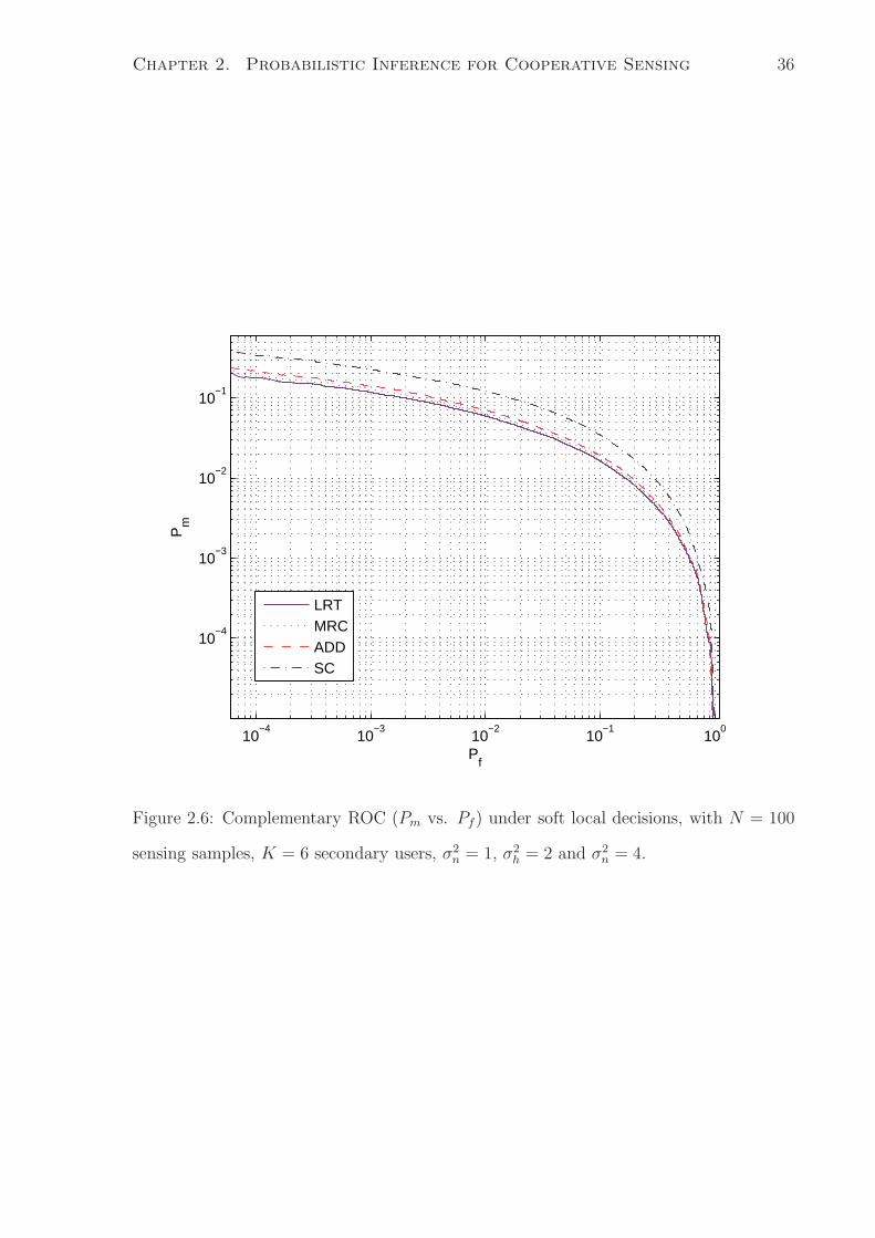
Chapter 2. Probabilistic Inference for Cooperative Sensing 36
10−4
10−3
10−2
10−1
100
10−4
10−3
10−2
10−1
Pf
Pm
LRTMRCADDSC
Figure 2.6: Complementary ROC (Pm vs. Pf) under soft local decisions, with N = 100
sensing samples, K = 6 secondary users, σ2n = 1, σ2
h = 2 and σ2n = 4.

Chapter 2. Probabilistic Inference for Cooperative Sensing 37
10−4
10−3
10−2
10−1
10−4
10−3
10−2
10−1
100
Pf
Pm
AND2K/3−out−of−KK/2−out−of−KK/3−out−of−KLRT, one−bitLRT, two−bit
Figure 2.7: Complementary ROC (Pm vs. Pf) under quantized local decisions,
with N = 500 sensing samples, K = 6 secondary users, σ2h
K
1 = σ2n
K
1 , σ2n
K
1 =
{1.28, 0.32, 4.5, 0.5, 2, 0.08}, and αK1 = {0.1, 0.3, 0.2, 0.05, 0.1, 0.2}.
Chapter 2. Probabilistic Inference for Cooperative Sensing 38
performs the aforementioned schemes by having a lower probability of missed detection
for the same probability of false alarm.
Figure 2.7 depicts the complementary ROC curves for a two-bit quantized local de-
cision scenario. The quantization thresholds are set to be a1k = τk/2, a2k = τk and
a3k = 2τk, where τk is determined as (2.23). The primary signal is assumed to be 4-
ASK modulated with maximum transmit voltage of A = 1. The M-out-of-K and hard
(one-bit) local decision LRT are provided for comparison. We observe that the two-bit
quantized LRT scheme significantly outperforms the one-bit quantized LRT and M-out-
of-K schemes.
2.6 Chapter Summary
In this chapter, we presented a probabilistic inference approach for cooperative spectrum
sensing by modeling the decision fusion in cooperative sensing as a probabilistic infer-
ence problem on a factor graph. This approach allows for modeling and accommodating
the uncertainties and correlations in the cooperative sensing system and applying the
well-known algorithms such as belief propagation for inferring the target probability dis-
tribution. Using belief propagation approach, we derived the LRT at the fusion center for
hard, soft and quantized local decision scenarios. Considering nonideal noisy channels,
we showed that the LRT cooperative sensing scheme outperforms conventional schemes
such as AND, OR and M-out-of-K rules and MRC and SC schemes. Unlike the hard de-
cision based methods that can only have a certain performance for fixed local thresholds,
the LRT method allows for achieving a wide range of performance by changing the global
threshold. We also showed that the quantized local decisions can considerably improve
the detection performance of the cognitive radios compared to the hard (one-bit) decision
scenario.
As shown in this chapter, the optimal LRT requires the knowledge of the primary

Chapter 2. Probabilistic Inference for Cooperative Sensing 39
signal and channel gains statistics which may not be available to the secondary users. In
the next chapter, we present a new scheme overcome this problem.

Chapter 3
Cooperative Spectrum Sensing with
Unknown Parameters
3.1 Introduction
As we showed in the previous chapter, the optimal LRT decision rule depends on the
statistics of the primary signal and channel gains. However, in cognitive radios such
information may not be readily available to the secondary users and the fusion cen-
ter. Therefore, in this chapter we investigate the problem of spectrum sensing with
unknown parameters. We consider the problem of spectrum sensing at a central node in
a cooperative-sensing cognitive radio network, acting analogously to the fusion center in
a distributed sensor network. The channels between the K sensing nodes or secondary
users and the FC are treated as noisy. The primary network, when active, is assumed to
transmit a zero-mean signal unknown to the cognitive network, which is received over a
Rayleigh flat-fading channel by each secondary user.
When the second- and fourth-order moments of the primary signal and the variance
of channel gains are known, we will show that it is possible to derive the NP test at
40

Chapter 3. Cooperative Sensing with Unknown Parameters 41
the FC based on various ways1 of making local decisions from the observations at the
sensing nodes. These results are derived using general concepts introduced in the context
of sensor networks [40,49,52–55], specialized to the scenario we just described. However,
in practice, it is unlikely that the SUs or the FC would have knowledge of the moments
of the transmitted primary signal or the channel between the primary transmitter and
each secondary user. In fact, this is an important constraint in cognitive radio networks.
Thus we go on to address the above problem, using first the notion of the general-
ized likelihood ratio test (GLRT) and its asymptotically (as the number of observations
increase without bound) equivalent form, and then further simplifying it heuristically to
the sum of log-likelihood derivatives. The resulting test statistic, which we call the linear
test statistic, does not require maximum likelihood estimates (MLEs) of the unknown
parameters, which are hard to derive analytically in many realistic scenarios, while show-
ing a comparable performance to the known-parameter optimal NP test. Compared to
other well-known asymptotically-equivalent tests to GLRT, such as the Wald and Rao
tests [56], this scheme is much simpler and does not require the calculation of the Fisher
information matrix which is not easily attainable or invertible in many practical scenarios.
The proposed simplified linear test is applied to the cases of (i) unknown primary
signal and PU-SU channel statistics, and (ii) unknown primary signal statistics but known
PU-SU channel statistics. In case (ii), for the practical case of weak constant-modulus
primary signals, we additionally derive the LMP test [56]. Furthermore, for threshold
setting and performance analysis, we derive the distributions of the linear test and LMP
statistics under the null hypothesis. In this chapter, we consider soft (infinite-precision)
and quantized local decision scenarios and derive the LRT and linear test statistics for
each case. Our simulation results demonstrate the close performance of the linear test to
the known-parameter LRT, without requiring the knowledge or estimation of the primary
statistics. This chapter has been published in part in [57] and [58].
1Binary, M -level and no quantization of the received signal energy.

Chapter 3. Cooperative Sensing with Unknown Parameters 42
...
PrimaryUser
User 1
User K
z
Secondary
Secondary
Fusion
γ0(.)Center
γ1(.)
γK(.)
p(y1|u1)
p(yK |uK)
n1
nK
u0
u1
uK
x1
xK
y1
yK
h1
hK
Figure 3.1: Block diagram of cooperative spectrum sensing system with K secondary
users.
The remainder of this chapter is organized as follows. The system model and the
NP-based LRT at the fusion center are presented in Section 3.2. The proposed linear
test for cooperative spectrum sensing is presented in Section 3.3. Section 3.4 comprises
the derivation of the linear test statistics for different types of local decisions under the
unknown channel and primary signal statistics as well as the linear test and LMP statis-
tics for known channel statistics and unknown primary signal moments along with the
analytical threshold setting for linear test and LMP. Section 3.5 provides the simulation
results and, finally, Section 3.6 concludes the chapter.
3.2 Model and Formulation
3.2.1 System Model
We consider a centrally coordinated cognitive radio network with K secondary users. We
assume the same system model and parameters as in Chapter 2. Figure 3.1 depicts the
block diagram of the assumed system. The detailed system model is provided in Section
2.2.

Chapter 3. Cooperative Sensing with Unknown Parameters 43
3.2.2 NP-Based LRT at the Fusion Center
Spectrum sensing is a binary hypothesis testing problem. The optimal decision rule at
the fusion center in the sense of maximizing the probability of detection for a given
probability of false alarm is the NP-based LRT. This method decides H1 if and only if
L(yK1 ) =
p(yK1 |z 6= 0)
p(yK1 |z = 0)
> λ, (3.1)
where the threshold λ is found by solving (numerically or analytically)
Pf =
∫
yK1 :L(yK
1 )>λ
p(yK1 |z = 0)dyK
1 (3.2)
for a given desired probability of false alarm Pf . We can apply the graphical model
approach for cooperative sensing presented in Chapter 2 to obtain the likelihood functions
p(yK1 |z 6= 0) and p(yK
1 |z = 0), for different system model assumptions. We showed
in (2.21) that the likelihood functions depend on E[|xk|2] and var[|xk|2] which were
derived in (2.19) and (2.20). It can be observed from (2.19) and (2.20) that E[|xk|2]
and var[|xk|2] depend on the second and forth order statistics of the primary signal and
channel gain variances. Therefore, LRT-based methods are only applicable when E[|xk|2]
and var[|xk|2] are known, in particular, when the second and forth order statistics of the
primary signal and channel gain variances are known.
3.3 The Proposed Composite Hypothesis Testing Ap-
proach
As discussed in Section 3.2.2 the optimal NP-based method relies on knowledge of the
primary signal and channel statistics. In practice, however, such knowledge may not
be available to the cognitive radios and thus, the LRT-based schemes are not directly
applicable. Therefore, in cognitive radios, detection schemes that are robust to unknown
parameters should be employed. In a general scenario, we assume that no knowledge

Chapter 3. Cooperative Sensing with Unknown Parameters 44
of the primary signal statistics and channel gains is available at the fusion center. We
denote β1,k = σ2hk
E[|z|2] and β2,k = σ4hk
E[|z|4], for k = 1, . . . , K, as the unknown pa-
rameters in the likelihood ratio in (3.1). The vector of unknown parameters is then
β = (β1,1, . . . , β1,K , β2,1, . . . , β2,K).
A well-known composite hypothesis test which can replace the NP-based LRT in
unknown parameter scenarios is the GLRT. Unlike the NP-based LRT, the GLRT is not
optimal but has been found to work well in many scenarios. This test first finds the MLE
of the unknown parameters under H1, and then forms the GLRT statistic:
LG(yK1 ) =
p(yK1 |β = β̂,H1)
p(yK1 |β = 0,H0)
(3.3)
where β̂ = arg maxβ p(yK1 |β,H1).
For finding β̂, we can maximize p(yK1 |β) over the entire parameter space rather than
merely over H1 (see [56], pg. 232), since the probability of the MLE yielding the particular
value 0 is zero. Therefore β̂ is the unrestricted MLE of β. The unrestricted MLE of β
attains the Cramer-Rao lower bound, assuming the asymptotic pdf of the MLE is attained
(see [56], pg. 232), thus it satisfies [28, 56]
∂ ln p(yK1 |β)
∂β= I(β)(β̂ − β) (3.4)
The ith element of∂ ln p(yK
1 |β)
∂βis given by [56],
∂ ln p(yK1 |β)
∂βi
=
K∑
j=1
[I(β)]ij(β̂j − βj) (3.5)
By the first-order Taylor expansion
[I(β)]ij = [I(β̂)]ij +∂[I(β)]ij
∂β
∣
∣
∣
T
β=β̂(β − β̂), (3.6)
we have
∂ ln p(yK1 |β)
∂βi
=
K∑
j=1
[I(β̂)]ij(β̂j − βj) +
K∑
j=1
∂[I(β)]ij
∂β
∣
∣
∣
βT =β̂(β − β̂)(β̂j − βj) (3.7)

Chapter 3. Cooperative Sensing with Unknown Parameters 45
By consistency of the unrestricted MLE [28,56,59], as K → ∞, β̂ → β, and thus the last
term which is of second order may be neglected [56]. Thus we have
∂ ln p(yK1 |β)
∂β= I(β̂)(β̂ − β) (3.8)
Integrating both sides of (3.8) with respect to β results in
ln p(yK1 |β) = (β̂ − β)T I(β̂)(β̂ − β) + C. (3.9)
The constant C is bound to be ln p(yK1 |β̂). Therefore the asymptotic likelihood function
is
p(yK1 |β) = p(yK
1 |β̂) exp
(
−1
2(β̂ − β)T I(β̂)(β̂ − β)
)
(3.10)
By replacing p(yK1 |β̂) from (3.10) into (3.3), the GLRT statistic reduces to
LG(yK1 ) =
p(yK1 |β = β̂)
p(yK1 |β = 0)
=1
exp(
−12β̂
TI(β̂)β̂
) (3.11)
Therefore, the asymptotic equivalent for GLRT can be represented as
2 lnLG(yK1 ) = β̂
TI(β̂)β̂ (3.12)
By substituting (3.8) into the asymptotic form of the GLRT in (3.12), the proposed
asymptotically equivalent test to GLRT is derived as
TL(yK1 ) = β̂
T ∂ ln p(yK1 |β)
∂β
∣
∣
∣
β=0
. (3.13)
We call the proposed test as the linear test as its test statistic consists of a linear com-
bination of∂ ln p(yK
1 |β)
∂βi
∣
∣
∣
β=0
terms. For the set of unknown parameters in our model, the
linear test statistic can be written as
TL(yK1 ) =
K∑
k=1
β̂1,k
∂ ln p(yK1 |β)
∂β1,k
∣
∣
∣
β=0+
K∑
k=1
β̂2,k
∂ ln p(yK1 |β)
∂β2,k
∣
∣
∣
β=0(3.14)

Chapter 3. Cooperative Sensing with Unknown Parameters 46
In scenarios where it is infeasible or computationally demanding to solve
∂ ln p(yK1 |β)
∂β= 0 (3.15)
uniquely for β under H1, we alternatively propose to substitute the β̂ vector with a vector
of ones, 1,
TL(yK1 ) = 1
T∂ ln p(yK
1 |β)
∂β
∣
∣
∣
β=0
. (3.16)
This choice is intuitive as we assume no prior knowledge about the known parameters
and when the MLEs are not available, they can be treated equally and the effect of all the
MLEs in (3.14) can be equalized. This simplified test can also be treated as a generalized
LMP with multiple unknown parameters. In our system model, the unknown parameters
are non-negative which removes the necessity of the quadratic form in the test statistic
and allows for a linear test statistic as in (3.16). Our numerical results support this
suggested scheme and show a close performance for the proposed linear scheme to that of
the optimal NP-based LRT with known parameters. This simplified linear test statistic
for the assumed model can be rewritten as
TSL(yK1 ) =
K∑
k=1
∂ ln p(yK1 |β)
∂β1,k
∣
∣
∣
β=0+
K∑
k=1
∂ ln p(yK1 |β)
∂β2,k
∣
∣
∣
β=0. (3.17)
This method can be used for any detection problem with unknown or uncertain param-
eters. Unlike the Rao and Wald tests (see Appendix C), the simplified linear test does
not have a quadratic form and does not require the calculation of the Fisher information
matrix which is a 2K × 2K matrix for our system. Therefore it is easier and faster to
implement compared to these schemes. In its simplified form (3.17), the linear test does
not even require the MLEs of the unknown parameters which results in a much simpler
and faster test compared to the Wald and GLRT tests. In fact, it is not feasible to
analytically find the unrestricted MLEs of unknown parameters in most realistic scenar-
ios [56], such as the soft and quantized local decision scenarios in this chapter. This linear
test is also much simpler than the Rao test which has a quadratic form and requires the

Chapter 3. Cooperative Sensing with Unknown Parameters 47
inverse of the Fisher information matrix. The Rao test, in fact, is not practical as the
Fisher information matrix is not easily attainable or invertible in many system models.
Dealing with multiple unknown parameters (in this case 2K parameters), exacerbates
the complexity and infeasibility of calculating this inverse matrix.
3.4 The Proposed Test for Cooperative Spectrum
Sensing
3.4.1 Unknown Primary Signal and Channel Statistics
In this section, we derive the NP-based LRT at the fusion center and apply the proposed
linear test to cooperative fusion of quantized and soft local decisions with unknown
primary signal moments and channel statistics.
Quantized Soft Local Decisions
In this section, we assume that the secondary users transmit locally quantized test statis-
tics (received signal energies) and then derive the LRT and linear test statistics at the
fusion center. In this chapter, we do not deal with the optimization of the local thresholds
and refer the readers to [40,49,52,54] for threshold optimization algorithms in distributed
sensor networks. We assume that the kth user quantizes its received signal energy with
Mk bits and preset local thresholds of a1k, . . . , a(Mk−1)k and sends uk ∈ {0, . . . , Mk − 1}
to the fusion center. In this case, the local decision sent to the fusion center based on
the quantized local energy is determined as follows:
uk = qi, if a(i−1)k < tk < aik for i = 1, . . . , Mk (3.18)

Chapter 3. Cooperative Sensing with Unknown Parameters 48
where qi = i − 1, a0k = 0 and aMkk = ∞. The likelihood function in this case is derived
in Appendix B as
p(yK1 |z) =
K∏
k=1
(
Mk∑
i=1
p(yk|qi)
[
Q
(
a(i−1)k − mtk
σtk
)
− Q
(
aik − mtk
σtk
)]
)
(3.19)
where Q(x) =∫∞
x1√2π
e−t2
2 dt and mtk and σ2tk
are respectively the mean and variance of
the local energy tk given as
mtk ,H1 = N(β1,k + σ2nk
), (3.20)
σtk ,H1 =√
N((2β2,k − β21,k) + 2β1,kσ2
nk+ σ4
nk). (3.21)
Consequently, the LRT statistic at the fusion center is derived as,
L(yK1 ) =
K∏
k=1
∑Mk
i=1 p(yk|qi)[
Q(
a(i−1)k−mtk,H1
σtk,H1
)
− Q(
aik−mtk,H1
σtk,H1
)]
∑Mk
i=1 p(yk|qi)
[
Q
(
a(i−1)k−Nσ2nk√
Nσ2nk
)
− Q
(
aik−Nσ2nk√
Nσ2nk
)] . (3.22)
We observe that the NP-based LRT depends on β1,k = σ2hk
E[|z|2] and β2,k = σ4hk
E[|z|4].
For M-ary PSK (phase shift keying) modulated primary signals, E[|z|2] = A2 and
E[|z|4] = A4, where A is the maximum transmit voltage. For M-ary ASK (amplitude
shift keying), we have
E[|z|2] =A2
3
M + 1
M − 1, (3.23)
E[|z|4] = A43M3 + 3M2 − 7M − 7
15(M − 1)3. (3.24)
Therefore, in order to apply the LRT, knowledge of the modulation type and maximum
transmit voltage of the primary signal as well as the channel gain variance is required at
the fusion center.
For the realistic scenario that the primary signal moments and channel statistics are
not available at the cognitive radios, we propose to apply the linear test rather than the
LRT in (3.22). For this reason, we derive the partial derivatives of the logarithm of the
LRT in (3.22) with respect to β1,k’s and β2,k’s and evaluate them at β = 0 as follows:

Chapter 3. Cooperative Sensing with Unknown Parameters 49
∂ ln p(yK1 |β)
∂β1,k
∣
∣
∣
β=0=
∑Mk
i=1 p(yk|qi)Aik1√
2πNσ4nk
∑Mk
i=1 p(yk|qi)
[
Q
(
a(i−1)k−Nσ2nk√
Nσ2nk
)
− Q
(
aik−Nσ2nk√
Nσ2nk
)] (3.25)
∂ ln p(yK1 |β)
∂β2,k
∣
∣
∣
β=0=
∑Mk
i=1 p(yk|qi)Bik2√
2πNσ6nk
∑Mk
i=1 p(yk|qi)
[
Q
(
a(i−1)k−Nσ2nk√
Nσ2nk
)
− Q
(
aik−Nσ2nk√
Nσ2nk
)] (3.26)
where
Aik = a(i−1)ke−
(a(i−1)k−Nσ2nk
)2
2Nσ4nk − aike
−(aik−Nσ2
nk)2
2Nσ4nk , (3.27)
Bik = [a(i−1)k − Nσ2nk
]e−
(a(i−1)k−Nσ2nk
)2
2Nσ4nk − [aik − Nσ2
nk]e
−(aik−Nσ2
nk)2
2Nσ4nk . (3.28)
Derivation of the MLEs of β1,k and β2,k is not feasible analytically in this scenario.
Therefore, we apply the simplified linear test and derive its test statistic as
TSL(yK1 )=
K∑
k=1
∑Mk
i=1p(yk|qi)√2πNσ4
nk
[
(a(i−1)k[1+ 2σ2
nk
]−2N)e−
(a(i−1)k−Nσ2nk
)2
2Nσ4nk −(aik[1+ 2
σ2nk
]−2N)e−
(aik−Nσ2nk
)2
2Nσ4nk
]
∑Mk
i=1 p(yk|qi)
[
Q
(
a(i−1)k−Nσ2nk√
Nσ2nk
)
−Q
(
aik−Nσ2nk√
Nσ2nk
)]
(3.29)
For the spacial case of binary (hard) local decisions, the LRT statistic in (3.22) reduces
to
L(yK1 ) =
K∏
k=1
p(yk|0) + [p(yk|1)−p(yk|0)]Q(
τk−mtk,H1
σtk,H1
)
p(yk|0) + [p(yk|1) − p(yk|0)]Q
(
τk−Nσ2nk√
Nσ2nk
) , (3.30)
where τk is the local threshold at the kth user. Based on the distribution of the local
energy in (2.18), the local threshold τk that result in local probability of false alarm of
pfkis determined as
τk = σ2nk
√NQ−1(pfk
) + Nσ2nk
. (3.31)
The linear test statistic at the fusion center, in this case, is obtained from (3.29) as
TSL(yK1 ) =
K∑
k=1
[p(yk|1) − p(yk|0)]e−
(τk−Nσ2nk
)2
2Nσ4nk
τkσ2nk
+2τk−2Nσ2nk√
2πNσ6nk
p(yk|0) + [p(yk|1) − p(yk|0)]Q
(
τk−Nσ2nk√
Nσ2nk
) . (3.32)

Chapter 3. Cooperative Sensing with Unknown Parameters 50
Soft Local Decisions
In many previous studies in cooperative sensing [17, 19, 21, 22] the local test statistics
(signal energies) were assumed to be transmitted with infinite precision to the fusion
center over error-free control channels. In this section, we derive the LRT and then the
linear test at the fusion center for such soft local decisions with noisy AWGN channels
from the users to the fusion center.
The signal received at the fusion center from the k-th sensor is yk = tk + wk, where
wk is assumed to be zero-mean Gaussian noise with variance σ2wk
, so that
p(yk|tk) =1√
2πσwk
exp
(
−(yk − tk)2
2σ2wk
)
. (3.33)
Given the Gaussian distribution of tk as in (2.18), yk is also Gaussian distributed under
H0 or H1:
yk ∼ N(
NE[|xk|2], Nvar[|xk|2] + σ2wk
)
, (3.34)
where E[|xk|2] and var[|xk|2] under H0 and H1, are given in (2.19) and (2.20) respectively.
Therefore, by independence of the channels, the LRT statistic is derived as follows:
L(yK1 ) =
K∏
k=1
p(yk|H1)
p(yk|H0)
=K∏
k=1
e−
(yk−N(β1+σ2nk
))2
2(N[(2β2−β21)+2β1σ2
nk+σ4
nk]+σ2
wk)+
(yk−Nσ2nk
)2
2(Nσ4nk
+σ2wk
)
√
N [(2β2−β21)+2β1σ2
nk+σ4
nk]+σ2
wk
Nσ4nk
+σ2wk
. (3.35)
The LRT decides H1 if L(yK1 ) > λ, where the threshold λ can be set using an empirical
distribution of the log-likelihood ratio under the null hypothesis.
We next derive the unknown-parameter linear test for soft local decisions by evaluating
the derivatives of the log-likelihood function at β = 0
∂ ln p(yK1 |β)
∂β1,k
∣
∣
∣
β=0=
N(yk − Nσ2nk
)(σ2nk
yk + σ2wk
)
(Nσ4nk
+ σ2wk
)2− 1
σ2nk
(3.36)
∂ ln p(yK1 |β)
∂β2,k
∣
∣
∣
β=0=
N(yk − Nσ2nk
)2
(Nσ4nk
+ σ2wk
)2− 1
σ4nk
(3.37)

Chapter 3. Cooperative Sensing with Unknown Parameters 51
and substituting (3.36) and (3.37) into (3.17). Solving∂ ln p(yK
1 |β)
∂β1,k= 0 and
∂ ln p(yK1 |β)
∂β2,k= 0
for β1,k and β2,k results in a third-order equation with respect to β1,k which must be
solved numerically. Thus, we alternatively use the simplified linear test for this scenario
and derive its statistic as
TSL(yK1 ) =
K∑
k=1
N(yk − Nσ2nk
)
(Nσ4nk
+ σ2wk
)2[yk(σ
2nk
+ 1) + σ2wk
− Nσ2nk
] −K∑
k=1
σ2nk
+ 1
σ4nk
. (3.38)
Note that TSL(yK1 ) depends on σ2
wkand σ2
nk, the AWGN variances in the SU-FC and
PU-SU channels respectively, but not on the primary transmitted signal statistics or the
PU-SU fading channel parameter.
3.4.2 Unknown Primary Signal Statistics and Known Channel
Statistics
Linear Test
It may be practical to assume that the second-order statistics of the channel gain from
the primary user to secondary users are available at the fusion center. Therefore, the
set of unknown parameters in our model will reduce to β1 = E[|z|2] and β2 = E[|z|4].
In this case, unlike in the previous section where the∂ ln p(yK
1 |β)
∂β1,k’s and
∂ ln p(yK1 |β)
∂β2,k’s only
consisted of terms that depend on k, the∂ ln p(yK
1 |β)
∂β1and
∂ ln p(yK1 |β)
∂β2consist of summations
of nonlinear terms in β1 and β2 over k. Therefore the analytical derivation of the MLEs
is infeasible for our general cooperative noisy channel model. Hence, we propose to apply
the simplified linear test with statistic
TSL(yK1 ) =
∂ ln p(yK1 |β)
∂β1
∣
∣
∣
β=0+
∂ ln p(yK1 |β)
∂β2
∣
∣
∣
β=0. (3.39)
From now on, we use the term linear test instead of the simplified linear test for concise-
ness. We can apply the linear test to all local decision scenarios discussed in Section 3.4.1
when the channel gain statistics are available but the primary signal statistics are not.

Chapter 3. Cooperative Sensing with Unknown Parameters 52
For the binary local decision scenario, for instance, the derivatives of the log-likelihood
ratio with respect to β1 and β2 are derived and evaluated at β = 0 as follows:
∂ ln p(yK1 |β)
∂β1
∣
∣
∣
β=0=
K∑
k=1
[p(yk|1)−p(yk|0)]e
−(τk−Nσ2
nk)2
2Nσ4nk σ2
hkτk√
2πNσ4nk
p(yk|0) + [p(yk|1)−p(yk|0)]Q
(
τk−Nσ2nk√
Nσ2nk
) , (3.40)
∂ ln p(yK1 |β)
∂β2
∣
∣
∣
β=0=
K∑
k=1
[p(yk|1) − p(yk|0)]e
−(τk−Nσ2
nk)2
2Nσ4nk 2σ4
hk(τk−Nσ2
nk)
√2πNσ6
nk
p(yk|0) + [p(yk|1) − p(yk|0)]Q
(
τk−Nσ2nk√
Nσ2nk
) . (3.41)
The linear test statistic in this case is derived by inserting (3.40) and (3.41) into (3.39).
We can similarly derive the linear test statistics of the soft and quantized local decisions
for known channel parameters and unknown primary signal statistics, but do not show
them here for conciseness.
LMP Test
When the channel gains are known and the only unknown parameters are the primary
signal statistics, we can use the LMP test under certain assumptions. The LMP test is
a one-sided scalar-parameter test for small departures of the parameter from zero [56].
The LMP test statistic is derived as
TLMP(yK1 ) =
∂ ln p(yK1 |β1,H1)
∂β1
∣
∣
∣
β1=0(3.42)
if β1 is the only unknown parameter. We use this scalar-parameter test for the case of
constant-modulus primary signal with unknown small power of β1. In this case, β2 = β21
and the only unknown parameter is β1. This test can be applied to hard, soft and
quantized local decision scenarios for constant-modulus primary signals. Here we derive
the LMP test statistic for the binary local decision case as an example. For constant-
modulus (e.g. M-PSK modulated) primary signals, the LRT statistic in (3.30) reduces

Chapter 3. Cooperative Sensing with Unknown Parameters 53
to
L(yK1 ) =
K∏
k=1
p(yk|0) + [p(yk|1) − p(yk|0)]Q
(
τk−N(β1σ2hk
+σ2nk
)√
N(β1σ2hk
+σ2nk
)
)
p(yk|0) + [p(yk|1) − p(yk|0)]Q
(
τk−Nσ2nk√
Nσ2nk
) . (3.43)
Therefore, the LMP test statistic is derived as
TLMP(yK1 ) =
K∑
k=1
[p(yk|1) − p(yk|0)]e−
(τk−Nσ2nk
)2
2Nσ4nk
σ2hk
τk√2πNσ4
nk
p(yk|0) + [p(yk|1) − p(yk|0)]Q
(
τk−Nσ2nk√
Nσ2nk
) . (3.44)
We observe that the LMP test statistic for weak constant-modulus primary signals has a
similar expression to the first part of the linear test statistic in (3.40) for general primary
signals. For the case of quantized local decisions, we derive the LMP test statistic as
TLMP(yK1 ) =
K∑
k=1
∑Mk
i=1 p(yk|qi)Aik
σ2hk√
2πNσ4nk
∑Mk
i=1 p(yk|qi)[
Q(
a(i−1)k−µtk
σtk
)
− Q(
aik−µtk
σtk
)] , (3.45)
where Aik is given in (3.27).
By and large, the proposed linear test can be applied for all ranges of signal power,
whereas the LMP is restricted to small signal powers. Moreover, the linear test accom-
modates multiple unknown parameters, while the LMP is confined to scalar parameter
tests.
3.4.3 Threshold Setting at the Fusion Center
Linear Test
In order to set the threshold at the fusion center when using the linear test, we need
the distribution of the test statistic TSL(yK1 ) under H0. Under H0 for which β = 0, by
regularity conditions [ [28], pg. 67] we have
E
[
∂ ln p(yK1 |β)
∂β
∣
∣
∣
β=0
]
= 0 (3.46)

Chapter 3. Cooperative Sensing with Unknown Parameters 54
and also
E
(
∂ ln p(yK1 |β)
∂β
∣
∣
∣
β=0
)2
= I(0) (3.47)
which is the Fisher information matrix at β = 0. Moreover, the linear test statistic can
be written as
TSL(yK1 ) =
K∑
k=1
∂ ln p(yK1 |β)
∂β1,k
∣
∣
∣
β=0+
K∑
k=1
∂ ln p(yK1 |β)
∂β2,k
∣
∣
∣
β=0. (3.48)
Therefore, by CLT we have
TSL(yK1 )∼N (0,
K∑
k=1
{Iβ1,k(0) + Iβ2,k
(0) + 2Iβ1,2,k(0)}), under H0 (3.49)
where
Iβi,k(0) = E
(
∂ ln p(yK1 |β)
∂βi,k
∣
∣
∣
β=0
)2
for i = 1, 2, (3.50)
and
Iβ1,2,k(0) = E
[(
∂ ln p(yK1 |β)
∂β1,k
∣
∣
∣
β=0
)(
∂ ln p(yK1 |β)
∂β2,k
∣
∣
∣
β=0
)]
. (3.51)
For binary local decisions and binary symmetric channels between the users and fusion
center, with crossover probability of αk, we derive Iβ1,k(0), Iβ2,k
(0) and Iβ1,2,k(0) as follows:
Iβ1,k(0) = (1 − 2αk)
2e−
(τk−Nσ2nk
)2
Nσ4nk
(
τk√2πNσ4
nk
)2
xk(1 − xk), (3.52)
Iβ2,k(0) = (1 − 2αk)
2e−
(τk−Nσ2nk
)2
Nσ4nk
(
2(τk−Nσ2nk
)√
2πNσ6nk
)2
xk(1 − xk), (3.53)
Iβ1,2,k(0) = (1 − 2αk)
2e−
(τk−Nσ2nk
)2
Nσ4nk
(
τk(τk−Nσ2nk
)
πNσ10nk
)
xk(1 − xk), (3.54)
where
xk = αk + (1 − 2αk)Q
(
τk − Nσ2nk√
Nσ2nk
)
. (3.55)

Chapter 3. Cooperative Sensing with Unknown Parameters 55
For the quantized local decision scenario, these information numbers can be derived as
Iβ1,k(0) =
M−1∑
yk=0
(
∑Mk
i=1 p(yk|qi)Aik1√
2πNσ4nk
)2
∑Mk
i=1 p(yk|qi)
[
Q
(
a(i−1)k−Nσ2nk√
Nσ2nk
)
− Q
(
aik−Nσ2nk√
Nσ2nk
)] , (3.56)
Iβ2,k(0) =
M−1∑
yk=0
(
∑Mk
i=1 p(yk|qi)Bik2√
2πNσ6nk
)2
∑Mk
i=1 p(yk|qi)
[
Q
(
a(i−1)k−Nσ2nk√
Nσ2nk
)
− Q
(
aik−Nσ2nk√
Nσ2nk
)] , (3.57)
Iβ1,2,k(0) =
M−1∑
yk=0
(
∑Mk
i=1 p(yk|qi)Aik1√
2πNσ4nk
)(
∑Mk
i=1 p(yk|qi)Bik2√
2πNσ6nk
)
∑Mk
i=1 p(yk|qi)
[
Q
(
a(i−1)k−Nσ2nk√
Nσ2nk
)
− Q
(
aik−Nσ2nk√
Nσ2nk
)] , (3.58)
where Aik and Bik are given in (3.27) and (3.28). Thus, using the derived distribution of
the linear test statistic under H0, the probability of false alarm for global threshold of λ
is given by
Pf = P{TSL(yK1 ) > λ|H0} (3.59)
= Q
λ√
∑K
k=1{Iβ1,k(0) + Iβ2,k
(0) + 2Iβ1,2,k(0)}
. (3.60)
In this way, we can analytically set the global threshold at the fusion center to maintain
the target probability of false alarm, Pf , as
λ = Q−1(Pf)
√
√
√
√
K∑
k=1
[Iβ1,k(0) + Iβ2,k
(0) + 2Iβ1,2,k(0)]. (3.61)
LMP Test
The LMP test statistic in (3.42) can be rewritten as
TLMP(yK1 ) =
K∑
k=1
∂ ln p(yk|β1,H1)
∂β1
∣
∣
∣
β1=0. (3.62)
Therefore, by CLT and regularity condition
E
[
∂ ln p(yk|β1)
∂β1
∣
∣
∣
β1=0
]
= 0, (3.63)
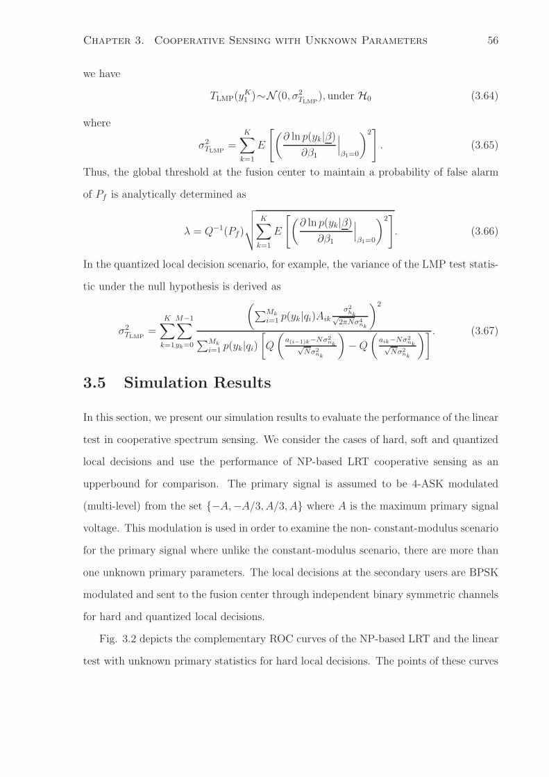
Chapter 3. Cooperative Sensing with Unknown Parameters 56
we have
TLMP(yK1 )∼N (0, σ2
TLMP), under H0 (3.64)
where
σ2TLMP
=
K∑
k=1
E
[
(
∂ ln p(yk|β)
∂β1
∣
∣
∣
β1=0
)2]
. (3.65)
Thus, the global threshold at the fusion center to maintain a probability of false alarm
of Pf is analytically determined as
λ = Q−1(Pf)
√
√
√
√
K∑
k=1
E
[
(
∂ ln p(yk|β)
∂β1
∣
∣
∣
β1=0
)2]
. (3.66)
In the quantized local decision scenario, for example, the variance of the LMP test statis-
tic under the null hypothesis is derived as
σ2TLMP
=K∑
k=1
M−1∑
yk=0
(
∑Mk
i=1 p(yk|qi)Aik
σ2hk√
2πNσ4nk
)2
∑Mk
i=1 p(yk|qi)
[
Q
(
a(i−1)k−Nσ2nk√
Nσ2nk
)
− Q
(
aik−Nσ2nk√
Nσ2nk
)] . (3.67)
3.5 Simulation Results
In this section, we present our simulation results to evaluate the performance of the linear
test in cooperative spectrum sensing. We consider the cases of hard, soft and quantized
local decisions and use the performance of NP-based LRT cooperative sensing as an
upperbound for comparison. The primary signal is assumed to be 4-ASK modulated
(multi-level) from the set {−A,−A/3, A/3, A} where A is the maximum primary signal
voltage. This modulation is used in order to examine the non- constant-modulus scenario
for the primary signal where unlike the constant-modulus scenario, there are more than
one unknown primary parameters. The local decisions at the secondary users are BPSK
modulated and sent to the fusion center through independent binary symmetric channels
for hard and quantized local decisions.
Fig. 3.2 depicts the complementary ROC curves of the NP-based LRT and the linear
test with unknown primary statistics for hard local decisions. The points of these curves

Chapter 3. Cooperative Sensing with Unknown Parameters 57
10−2
10−1
10−3
10−2
10−1
100
Pf
Pm
Linear testLRT
A2=4
A2=2
Figure 3.2: Complementary ROC (Pm vs. Pf) curves for hard local decisions with un-
known primary statistics and K = 3.
are achieved by changing the global threshold at the fusion center. We consider K = 3
secondary users in the network which independently sense the primary user’s spectrum.
The Rayleigh fading channel coefficients are assumed to be independently drawn from
CN (0, σ2hk
), where the variances σ2hk
s for the three PU-SU channels are assumed to be
0.32, 4.5 and 0.08 respectively. The local energy detection thresholds are chosen to achieve
a target local probability of false alarm of pf = 0.1, where the local noise variances are
set to be σ2n = σ2
h. The number of sensing samples are assumed to be N = 100. The
crossover probabilities for the six SU-FC BSC channels are 0.05, 0.1 and 0.05 respectively.
We observe that the linear test has performance close to that of the optimal NP-based
LRT fusion for the cases of both A2 = 2 and A2 = 4. In the first case β1 = 1.11 and

Chapter 3. Cooperative Sensing with Unknown Parameters 58
10−2
10−1
10−2
10−1
100
Pf
Pm
Linear testLRT
N=10N=100N=6
Figure 3.3: Complementary ROC (Pm vs. Pf) curves for hard local decisions with un-
known primary statistics and K = 3.
β2 = 2.02, whereas the difference between the two parameters is even higher in the second
case where β1 = 2.22 and β2 = 8.09.
Fig. 3.3 depicts the complementary ROC curves of the NP-based LRT and the linear
test with unknown primary statistics for hard local decisions and different values of N .
We consider K = 3 secondary users and the same channel and noise parameters as the
previous figure. We observe that the simplified linear test performs closely to the optimal
NP-based LRT fusion for small as well as large numbers of sensing samples.
Fig. 3.4 depicts the complementary ROC curves of the NP-based LRT and the linear
test with unknown primary statistics for hard local decisions. We consider K = 6 sec-
ondary users in the network which independently sense the primary user’s spectrum with
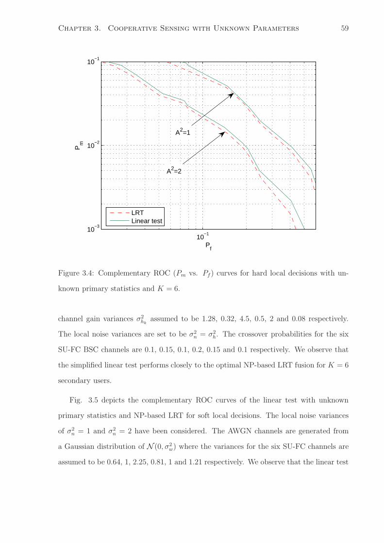
Chapter 3. Cooperative Sensing with Unknown Parameters 59
10−1
10−3
10−2
10−1
Pf
Pm
LRTLinear test
A2=1
A2=2
Figure 3.4: Complementary ROC (Pm vs. Pf) curves for hard local decisions with un-
known primary statistics and K = 6.
channel gain variances σ2hk
assumed to be 1.28, 0.32, 4.5, 0.5, 2 and 0.08 respectively.
The local noise variances are set to be σ2n = σ2
h. The crossover probabilities for the six
SU-FC BSC channels are 0.1, 0.15, 0.1, 0.2, 0.15 and 0.1 respectively. We observe that
the simplified linear test performs closely to the optimal NP-based LRT fusion for K = 6
secondary users.
Fig. 3.5 depicts the complementary ROC curves of the linear test with unknown
primary statistics and NP-based LRT for soft local decisions. The local noise variances
of σ2n = 1 and σ2
n = 2 have been considered. The AWGN channels are generated from
a Gaussian distribution of N (0, σ2w) where the variances for the six SU-FC channels are
assumed to be 0.64, 1, 2.25, 0.81, 1 and 1.21 respectively. We observe that the linear test

Chapter 3. Cooperative Sensing with Unknown Parameters 60
10−3
10−2
10−1
10−4
10−3
10−2
10−1
Pf
Pm
Linear testLRT
σ2
n= 1
σ2
n= 2
Figure 3.5: Complementary ROC (Pm vs. Pf) curves for soft local decisions and K = 6.
performs closely to the optimal NP-based LRT fusion for the soft local decision scenario.
Fig. 3.6 depicts the complementary ROC curves of NP-based LRT and the linear test
with unknown primary statistics for 2-bit quantized local decisions. The quantization
thresholds are set to be a1k = τk/2, a2k = τk and a3k = 2τk, where τk is determined as
(3.31) for pf = 0.05, and A is assumed to be 0.8. The crossover probabilities of α = 0.05
and α = 0.1 are considered for the BSC SU-FC channels. We observe that the linear test
performs closely to the optimal NP-based LRT.
Fig. 3.7 depicts the complementary ROC curves of NP-based LRT and linear test
with unknown channel gains and primary statistics for 2-bit quantized local decisions.
The BSC cross-over probabilities of 0.1 and 0.05, local noise and channel gain variance of
1 and maximum transmit voltage of 1 have been assumed. We observe that the linear test

Chapter 3. Cooperative Sensing with Unknown Parameters 61
10−3
10−2
10−1
10−2
10−1
Pf
Pm
LRTLinear test
α = 0.05
α = 0.1
Figure 3.6: Complementary ROC (Pm vs. Pf) curves for 2-bit quantized local decisions
with unknown primary statistics.
performs comparably to the optimal NP-based LRT with known primary and channel
parameters. As the channel gain variance is not known to the FC, the performance
gap between the LRT and the linear test is more considerable compared to the previous
figure. Our simulation results show that with knowledge of the channel gain variance at
the FC, the performance of the linear test becomes closer to that of the LRT.
Fig. 3.8 shows the analytical and numerical probability distribution of the linear test
statistic under the null hypothesis. We observe that the analytical pdf derived in (3.49)
is very close to the numerical pdf which represents the exact pdf.

Chapter 3. Cooperative Sensing with Unknown Parameters 62
10−4
10−3
10−2
10−1
10−2
10−1
100
Pf
Pm
Linear testLRT
α = 0.05
α = 0.1
Figure 3.7: Complementary ROC (Pm vs. Pf) curves for 2-bit quantized local decisions
with unknown primary and channel gain statistics.
3.6 Chapter Summary
In this chapter, we presented a composite hypothesis testing approach for cooperative
spectrum sensing in cognitive radios. For non-ideal transmission channels, we derived
the LRT statistic based on the Neyman-Pearson criterion at the fusion center. However,
due to lack of knowledge about the primary signal and channel statistics at the secondary
networks, the optimal LRT-based scheme which depends on these parameters, cannot be
applied in most cognitive radio networks. For this reason, we proposed linear composite
hypothesis testing methods, which do not require any prior knowledge about the primary
signal and channel statistics. In its simplified form, this test is more practical and simpler
compared to the GLRT which requires ML estimates of the unknown parameters. We

Chapter 3. Cooperative Sensing with Unknown Parameters 63
−20 −15 −10 −5 0 5 10 15 200
0.02
0.04
0.06
0.08
0.1
0.12
0.14
0.16
0.18
0.2
TSL
(y1K)
Numerical pdfAnalytical pdf
Figure 3.8: Probability distribution function of the linear test statistic under the null
hypothesis.
derived the linear test statistic for decision making at the fusion center under hard, soft
and quantized local decision scenarios. Furthermore, we applied the LMP detector at the
fusion center for weak constant-modulus primary signals and derived its corresponding
test statistic. Deriving the pdf of the linear test and LMP statistics under the signal-
absent hypothesis, we analytically determined the linear test and LMP thresholds at the
fusion center. We showed that applying the linear test for cooperative sensing results in
very close performance to that of the known-parameter NP-based LRT, without requiring
prior knowledge of the primary statistics at the fusion center.

Chapter 4
Cooperative Quickest Spectrum
Sensing with Unknown Parameters
A large and growing body of work on spectrum sensing is focused on block detection meth-
ods, in which the detector makes its decision based on a window or block of observations,
using classical statistical detection theory (see e.g. [9,10,17–19,21–24]). However, in prac-
tice, changes in primary-network activity within the frequency band of interest should
be sensed as quickly as possible, in order to maximally utilize any vacated spectrum, as
well as to minimize interference to the primary network after it resumes transmission.
Therefore, detection delay is an important criterion in spectrum sensing, especially in
bursty primary networks.
Sequential change-point detection (quickest detection) provides a theoretical frame-
work for minimizing detection delay, and is therefore well-matched to spectrum sensing
in cognitive radios [30]. The well-known Page’s cumulative sum (CUSUM) algorithm [33]
has been shown to be optimal in the sense of minimizing the detection delay while main-
taining an acceptable level of false alarm [34]. The CUSUM algorithm was applied to
spectrum sensing, in the context of a single sensor, in [30] and [31]. However, at low
SNRs, spectrum sensing based on a single user’s observations may not be reliable, and a
64

Chapter 4. Cooperative Quickest Sensing with Unknown Parameters 65
diversity of sensors at various locations is known to give better results through coopera-
tive or collaborative sensing.
In this chapter, we first present cooperative quickest spectrum sensing schemes based
on the CUSUM algorithm. The study of distributed quickest detection has been based
on two different formulations in the detection literature. One is based on a Bayesian
formulation in which the change point (i.e. time at which the change occurs) is assumed
to have a known prior distribution [60]. In this case, the joint optimization of local users
and the fusion center policies over time becomes intractable [37]. The other formula-
tion is the minimax formulation, proposed by Lorden [34], for which Page’s CUSUM
procedure is the optimal scheme. The asymptotically optimal decentralized CUSUM ap-
proaches for limited and full local memory scenarios have been studied by Mei [37]. In
this chapter, we apply and compare three CUSUM-based cooperative spectrum sensing
schemes in cognitive radios mainly based on Mei’s studies [37]: global CUSUM with soft
local decisions, global CUSUM with quantized local decisions and hard fusion of local
CUSUM. We derive the local and global test statistics in each scheme assuming noisy
channels between the secondary users and the fusion center.
Next, we address the issue of limited knowledge about the primary signal at the
secondary users. In particular, when the primary user starts transmission, there are
unknown parameters in the distribution of the observed signals, e.g. the variance of the
observed signals, due to unknown primary signal statistics and channel gains between the
primary and secondary users. Therefore, the CUSUM-based approaches that are based on
perfectly known distributions cannot be directly applied to spectrum sensing in cognitive
radios. The generalized likelihood ratio test (GLRT) was adopted by Lorden [15] for
CUSUM with unknown parameters. However, due to the non-recursive expression of
the GLRT-based CUSUM and the need to store all the observations and re-estimate
the unknown parameters in all time slots, this algorithm turns out to be infeasible and
impractical.

Chapter 4. Cooperative Quickest Sensing with Unknown Parameters 66
As an alternative, we propose a linear test for quickest spectrum sensing which does
not require maximum likelihood (ML) estimates of the unknown parameters and has the
same asymptotic performance as the GLRT. We derive the test statistics of the linear test
version of the CUSUM-based cooperative sensing schemes and show that the CUSUM-
based schemes using the linear test perform comparably to the optimal CUSUM-based
schemes, without requiring knowledge of the primary signal or channel gains. Unlike the
successive refinement algorithm in [31] and the adaptive parameter tracking approach
in [61], our scheme does not require any iterative algorithm or any parameter estimation
and, thus, it is much faster and less complex to implement. It has also a much simpler
implementation and much better performance compared to the nonparametric algorithm
adopted in [30].
For performance evaluation and threshold setting, we apply the matrix approach
in [62] which is based on finding the cumulative distribution function (CDF) of the
stopping time through an underlying state-update process. We provide the threshold-
setting scheme for both known and unknown-parameter CUSUM-based algorithms. This
chapter has been partly published in [63].
The remainder of this chapter is organized as follows. The system model is described
in Section 4.1. The CUSUM-based cooperative quickest sensing schemes with known
parameters are presented in Section 4.2. The cooperative quickest detection schemes
with unknown parameters are presented in Section 4.3 where the linear test is applied
to the CUSUM-based schemes. The threshold setting scheme is described in Section 4.4.
The simulation results are provided in Section 4.5. Finally, Section 4.6 concludes the
chapter.

Chapter 4. Cooperative Quickest Sensing with Unknown Parameters 67
4.1 System Model
We assume L secondary users are monitoring the frequency band allocated to the primary
user. Let xl,i denote the observation at the lth secondary user at time i. When the
primary user is not active xl,i = nl,i, where nl,i is zero-mean white Gaussian noise with
variance σ2nl
. When the primary user is using the band xl,i = zl,i + nl,i, where zl,i is
the faded received primary signal at the lth secondary user. We assume time-invariant
channel gain hl between the primary user and the lth secondary user, and zl,i = hlsi to
be zero-mean Gaussian with variance σ2zl.
In this chapter, we focus on the detection of the emergence of the primary signal in the
band. The detection of vacancy in the band can be tackled similarly as we discuss in the
next chapter. We assume that the primary user is initially inactive, and at an unknown
time τ it becomes active. Thus there is a change in the distribution of the observations
from N (0, σ2nl
) to N (0, σ2zl
+ σ2nl
) at unknown time τ . The sequential change detection
modeling of this problem is to detect this change as quickly as possible while maintaining
a certain false alarm probability. Defining the detection time T as the time at which the
change is detected, if T > τ then the detection delay is δ = T −τ . If T < τ , a false alarm
has occurred with the average run length (ARL) of false alarm being Tf = E[T |T < τ ].
The detection of the primary user vacating the band can be approached similarly. The
non-Bayesian approach to this problem based on Lorden’s formulation [34] minimizes the
average detection delay,
Td = supτ≥1
Eτ [T − τ |T ≥ τ ] (4.1)
while maintaining the ARL of false alarms larger than a certain threshold, Tf ≥ λ.
The algorithm that finds the minimum Td in this problem, is Page’s CUSUM algorithm
(a.k.a. the Page test) [33]. The stopping time in this algorithm for a single user detection
problem is determined as follows:
T (q) = inf{n : Cn ≥ q} (4.2)
Chapter 4. Cooperative Quickest Sensing with Unknown Parameters 68
with cumulative statistic
Cn = max1≤k≤n
n∑
i=k
Li(xi) (4.3)
where
Li(xi) = logf1(xi)
f0(xi)(4.4)
and f0(xi) and f1(xi) are the distributions of xi before and after the change, respectively.
The cumulative statistic Cn can be recursively calculated for n ≥ 1 as follows:
Cn = max(Cn−1, 0) + Ln(xn) (4.5)
where C0 = 0. In other words, this algorithm finds the first n for which Cn ≥ q > 0.
The only analytical results on quickest detection performance bounds and their relations
to the threshold q deal with asymptotic scenarios where q → ∞ [29, 37], which are not
practical. The analysis in [37] may be used to asymptotically bound the performance of
the schemes in the next section.
4.2 Cooperative CUSUM with Full Knowledge of
Parameters
Due to fading and shadowing effects in cognitive radio networks, detection performance
improves with the number of available sensors that make independent observations. In
this section, we introduce cooperative quickest sensing schemes for cognitive radios, given
full knowledge of all parameters. We apply CUSUM-based approaches mainly based
on [37] to various local memory and transmission rate scenarios, and derive the necessary
test statistics. In all these methods, the local decisions are sent to a decision making
fusion center, which makes the global final decision. In the next section, we will tackle
the problem of unknown parameters.

Chapter 4. Cooperative Quickest Sensing with Unknown Parameters 69
4.2.1 Global CUSUM
Assuming noiseless error-free channels between the secondary users and the fusion center,
the local observations can be completely provided to the fusion center. Thus, the global
CUSUM can be applied at the fusion center based on the local observations. In this case,
based on [37], the CUSUM test statistic at the fusion center can be written as
Cn = max1≤k≤n
n∑
i=k
L∑
l=1
Lli(xl,i). (4.6)
where Lli(xl,i) represents the log-likelihood function at time i at the lth user. In our
assumed model, f l0(xl,i) = 1√
2πσnl
e−
x2l,i
2σ2nl and f l
1(xl,i) = 1√2π(σ2
nl+σ2
zl)e−
x2l,i
2(σ2nl
+σ2zl
) , thus the
global CUSUM statistic is derived as
Cn = max1≤k≤n
n∑
i=k
L∑
l=1
(
1
2log
(
σ2nl
σ2nl
+σ2zl
)
+x2
l,iσ2zl
2σ2nl
(σ2zl
+σ2nl
)
)
. (4.7)
The fusion center declares that the primary user is active as soon as Cn exceeds threshold
q. In practice, due to communication constraints in cognitive radios, the exact local
observations cannot be completely provided to the fusion center. Therefore, we consider
the quantized local observation scenario in the next section.
4.2.2 Global CUSUM with Quantized Local Decision
The case of unlimited bandwidth between the fusion center and the secondary users have
been considered in the previous section. However, bandwidth constraints in wireless
communications implies quantization of the local observations before they are sent to
the fusion center. For memoryless local users, it has been shown that the monotone
likelihood ratio quantizer (MLRQ) is the optimal local mapping [37]. In this mapping,
the lth user local decision at time n is Ul,n = d if and only if
al,d ≤ f1(xl,n)
f0(xl,n)< al,d+1 (4.8)

Chapter 4. Cooperative Quickest Sensing with Unknown Parameters 70
where 0 = al,0 . . . ≤ al,Dl−1 ≤ al,Dl= ∞ are the lth user quantization thresholds.
These local decisions are sent to the fusion center over noisy channels characterized by
p(yl,k|Ul,k). The fusion center applies Page’s CUSUM scheme with stopping time
T (q) = inf{n : Cn ≥ q} (4.9)
with C0 = 0 and
Cn = max(Cn−1, 0) +L∑
l=1
Lln(yl,n), (4.10)
where Lln(yl,n) is the log-likelihood ratio of yl,n at the fusion center. Using the graphical
approach in Chapter 2, we derive this log-likelihood ratio as follows:
Llk(yl,k)=log
∑Dl
d=1 p(yl,k|d)P [al,d−1 ≤ lr(xl,k) ≤ al,d|H1]∑Dl
d=1 p(yl,k|d)P [al,d−1 ≤ lr(xl,k) ≤ al,d|H0](4.11)
where lr(xl,k) =f1(xn,l)
f0(xn,1)and H0 and H1 represent xl,n ∼ N (0, σ2
nl) and xl,n ∼ N (0, σ2
nl+
σ2zl) respectively. In order to calculate P [al,d−1 ≤ lr(xl,k) ≤ al,d|Hθ], for θ = 1, 2, we need
to translate the MLRQ thresholds into thresholds for the observations xl,k. For Gaussian
distributed local observations, the likelihood ratio is derived as
lr(xl,k) =σnl
√
σ2nl
+ σ2zl
exp
(
σ2zlx2
l,k
(σ2nl
+ σ2zl)σ2
nl
)
. (4.12)
Thus, lr(xl,k) ≥ al,k is equivalent to
x2l,k ≥ log
(
al,d
√
σ2nl
+ σ2zl
σnl
)
(σ2nl
+ σ2zl)σ2
nl
σ2zl
(4.13)
where the right hand side of the inequality (4.13) is the equivalent threshold for x2l,k, which
we call a′l,d. Given the Gaussian distribution of xl,k, x2
l,k will be exponentially distributed
with parameters 2σnland 2
√
σ2nl
+ σ2zl, under H0 and H1 respectively. Therefore,
P [a′l,d−1≤x2
l,k ≤ a′l,d|H0] = e
−a′
l,d−12σnl −e
−a′
l,d
2σnl ,
P [a′l,d−1≤x2
l,k ≤ a′l,d|H1] = e
−a′
l,d−1
2√
σ2nl
+σ2zl−e
−a′
l,d
2√
σ2nl
+σ2zl .

Chapter 4. Cooperative Quickest Sensing with Unknown Parameters 71
Consequently, the log-likelihood ratio is derived as
Llk(yl,k)=log
∑Dl−1d=0 p(yl,k|d)[e
−a′
l,d
2√
σ2nl
+σ2zl −e
−a′
l,d+1
2√
σ2nl
+σ2zl ]
∑Dl−1d=0 p(yl,k|d)[e
−a′
l,d2σnl −e
−a′
l,d+12σnl ]
. (4.14)
For the case of binary local decisions with thresholds a′l, the likelihood ratio becomes
Llk(yl,k)=log
p(yl,k|0) + [p(yl,k|1) − p(yl,k|0)]e− a′
l
2√
σ2nl
+σ2zl
p(yl,k|0) + [p(yl,k|1) − p(yl,k|0)]e− a′
l2σnl
. (4.15)
The algorithm stops and the presence of the primary user is detected right after Cn ≥ q.
4.2.3 Hard Fusion of Local CUSUM
In this section we assume that each secondary user has sufficient memory to individually
perform the CUSUM algorithm and send its local decision to the fusion center. The
CUSUM test statistic at the lth user is derived as
C ln = max
1≤k≤n
n∑
i=k
Lli(xl,i), (4.16)
where the log-likelihood ratio Lli(xl,i) is derived as
Lli(xl,i) =
1
2log
(
σ2nl
σ2nl
+ σ2zl
)
+x2
l,iσ2zl
2σ2nl
(σ2zl
+ σ2nl
). (4.17)
After each update the lth user sends its local decision
Ul,n =
{
1 C ln ≥ ql
0 otherwise,(4.18)
to the fusion center. The fusion center can use any of the well-known hard-decision
combining schemes, such as OR, AND, M-out-of-L rules, to make the final decision. The
stopping time in the M-out-of-L rule scenario can be written as
T (q) = inf{n : C ln ≥ ql for at least M out of L users} (4.19)
where q = [q1, . . . , qL] captures all L users’ local thresholds.

Chapter 4. Cooperative Quickest Sensing with Unknown Parameters 72
4.3 Cooperative CUSUM with Unknown Parame-
ters
All the CUSUM-based approaches are based on perfect knowledge of the likelihood
functions. In cognitive radios, however, the parameters of the distribution under H1
are not known due to unknown primary signal statistics and channel gains. Therefore,
detection schemes that accommodate unknown parameters should be employed.
4.3.1 The GLRT for Quickest Detection
Lorden [34] proposed to apply the GLRT in CUSUM algorithms with uncertain param-
eters. Let us denote the unknown parameters by β. The GLRT replaces the unknown
parameter with its ML estimate. Thus the basic CUSUM statistic in (4.3) can be replaced
with
Cn = max1≤k≤n
maxβ
n∑
i=k
logf1(xi|β)
f0(xi). (4.20)
Equation (4.20) implies that we can no longer have a recursive expression for the CUSUM
as in (4.5), since the GLRT requires a re-calculation of β for each k, using all the obser-
vations up to the current time n. Thus, in practice, the GLRT approach is hard or even
infeasible to be implemented in CUSUM-based systems. Therefore, for quickest detection
schemes, we propose to use the asymptotically equivalent tests for GLRT that do not
require the ML estimate of the unknown parameters and are practical to implement.
4.3.2 The Rao Test for Quickest Detection Schemes
The Rao test is asymptotically equivalent to the GLRT, and does not require the ML
estimate of the unknown parameters thereby making it simpler computationally [15]. In
classical detection, the Rao test statistic for observation set x = {x1, . . . , xn} is given by
R(x) =∂ log f1(x|β)
∂β
∣
∣
∣
T
β=0I−1(0)
∂ log f1(x|β)
∂β
∣
∣
∣
β=0(4.21)

Chapter 4. Cooperative Quickest Sensing with Unknown Parameters 73
where I(0) is the Fisher information matrix (see [28] pg. 40) evaluated at β = 0. How-
ever, as the quadratic form implies the Rao test cannot result in a recursive expression
for the CUSUM as in (4.5) and thus, is not applicable to CUSUM-based approaches. The
calculation of the inverse Fisher information matrix, on the other hand, is computation-
ally demanding in multi-parameter scenarios. Therefore, in the next section we propose
a linear test which results in a recursive expression for the test statistic and is simple to
implement.
4.3.3 The Proposed Linear Test for Quickest Detection Schemes
The standard Rao test is a two-sided test, which necessitates the quadratic form in (4.20).
In our model, however, the unknown parameters are σ2zl
which are nonnegative. As a
result, the parameter test is one-sided which eliminates the necessity of the quadratic
form. Therefore, we propose a modified test with a linear statistic of
Λ(x) =
L∑
l=1
∂ log f1(x|βl)
∂βl
∣
∣
∣
βl=0. (4.22)
As (4.22) shows, the linear test replaces each log-likelihood ratio term depending on
βl, with its derivative at βl = 0 which distributes over the summation in CUSUM test
statistic unlike the ML estimation in the GLRT approach in (4.20). Therefore, unlike
GLRT-based approaches it does not require storing the observations and re-estimating
the parameters at every sampling interval. The linear test is easily applicable to CUSUM-
based algorithms, unlike the Rao test which has a quadratic form and does not allow for
a recursive expression for the test statistic.
In this section, we apply the linear test (4.22) to the cooperative CUSUM-based
schemes discussed in Section 4.2, when the received signal variances are not known upon
primary user activity. All the proposed linear-based schemes in this section, do not
require any iterative algorithm and any parameter estimation. As a result, they are faster
and less complicated compared to the successive refinement algorithm in [31] and the

Chapter 4. Cooperative Quickest Sensing with Unknown Parameters 74
nonparametric algorithm adopted in [30] which are applied for non-cooperative quickest
detection.
Global CUSUM with linear test
Although the primary signal and channel statistics may not be known at the fusion center,
we can still apply the global CUSUM algorithm by adopting the linear-based approach as
follows. By denoting βl = σ2zl
and replacing the lth log-likelihood ratio term in (4.7) with
its derivative with respect to βl evaluated at βl = 0, we derive the recursive linear-based
global CUSUM statistic as follows:
Cλn = max(Cλ
n−1, 0) +
L∑
l=1
1
2σ2nl
(
x2l,n
σ2nl
− 1
)
(4.23)
where Cλ0 = 0 and the superscript λ represents the linear test approach. The algorithm
will stop as soon as it finds the first n ≥ 1 that satisfies Cλn ≥ qλ.
Global CUSUM using quantized local decisions with linear test
The linear-based algorithm for global CUSUM with local MLRQ can be developed as
follows. We replace the lth log-likelihood ratio term in (4.10) with its derivative evaluated
at βl = 0 and derive the linear-based global CUSUM recursively as
Cλn = max(Cλ
n−1, 0) +L∑
l=1
Λln(yl,n) (4.24)
where
Λln(yl,n)=
∑Dl−1d=0 p(yl,n|d) 1
4σ3nl
[a′l,de
−a′
l,d2σnl −a′
l,d+1e−
a′l,d+12σnl ]
∑Dl−1d=0 p(yl,n|d)[e
−a′
l,d
2σnl −e−
a′l,d+12σnl ]
(4.25)
and Cλ0 = 0. The primary user is declared to be present right after Cλ
n goes beyond
threshold qλ.

Chapter 4. Cooperative Quickest Sensing with Unknown Parameters 75
Hard fusion of local CUSUM with linear test
When the secondary users have sufficient memory but no knowledge of the primary signal
and channel statistics, they can individually perform the linear-based CUSUM algorithm.
The test statistic at the lth user can be recursively derived by taking derivative from
(4.16) with respect to βl = σ2zl
and evaluating it at βl = 0:
Cλl,n = max(Cλ
l,n−1, 0) +1
2σ2nl
(
x2l,n
σ2nl
− 1
)
(4.26)
where Cλl,0 = 0. The lth user decision sent to the fusion center at time n is determined as
Uλl,n =
{
1 , Cλl,n ≥ qλ
l
0 , otherwise.(4.27)
The global stopping time depends on the combining rule at the fusion center. For OR
combining rule, for example, the algorithm stops as soon as Cλl,n exceeds qλ
l for at least
one of the users.
4.4 Performance Analysis and Threshold Setting
The performance of the standard Page test for detection of a one-time permanent change
has been studied in terms of average run length, mainly in asymptotic form [34]. In
cognitive radios, the probability of false alarm is a useful performance metric. The
probability of false alarm can be defined as P [T (q) < τ ], i.e., the probability that the
fusion falsely decides that the primary user has become active while it has not. Several
methods have been proposed in [62] for performance analysis of the Page test in terms
of probability of false alarm. These methods determine the CDF of the stopping time.
In this section, we use the matrix approach in [62] to find the probability of false alarm.
In this approach the Page’s test update (Ln(xn)) is uniformly quantized with a step size
of ∆. Let the quantization levels be li = i∆, i = 0,±1,±2, . . .. Let pni denote the
probabilities of the Page’s test update, Ln(xn), taking value li at time n, under H0.

Chapter 4. Cooperative Quickest Sensing with Unknown Parameters 76
We define a state vector un as the vector of probabilities of Ln(xn) lying in each
quantization level at time n, i.e.
un = [pn0 , p
n1 , . . . , p
nγ−1]
′ (4.28)
where γ is the integer satisfying lγ−1 < q < lγ for the test threshold q (i.e., γ is the
threshold index), the superscript ′ represents the matrix transpose operation, and
pni = Pr
{
i∆ − ∆
2≤ Ln(xn) < i∆ +
∆
2|H0
}
. (4.29)
As described in [62], the one step update can be written as
un+1 =Dnun
1′Dnun
, (4.30)
where 1 is a vector of ones and the square matrix Dn is
Dn =
∑0i=−∞ pn
i
∑−1i=−∞ pn
i . . .∑−(γ−1)
i=−∞ pni
pn1 pn
0 . . . pn−γ+2
pn2 pn
1 . . . pn−γ+3
......
. . ....
pnγ−1 pn
γ−2 . . . pn0
. (4.31)
The probability mass function of the quantized Page’s test statistic is contained in
un [64], which is given by
un = DnDn−1 . . .D0u0 (4.32)
where u0 is a vector composed of the initial probabilities of observing (l0, l1, . . . , lγ−1).
The CDF of the stopping time T which is the probability that the algorithm has
stopped prior to or during the current time sample can be written as [64]
FT (t) = 1 − Pr{Test update takes on levels (l0, l1, . . . , lγ−1) at time t}
= 1 − 1′DtDt−1 . . .D1u0 (4.33)
under H0. With the realistic assumption that the test starts with the zero state, u0 has a
one as the first element and zeros elsewhere, i.e. u0 = e1. When the sensing nonlinearity

Chapter 4. Cooperative Quickest Sensing with Unknown Parameters 77
does not change with time (as in our case), all the probability transition matrices will be
the same and equal to D and thus the CDF of the stopping time T , under H0, reduces
to
FT (t) = 1 − 1′Dte1 (4.34)
On the other hand, the probability of one or more false alarms in a signal of length nd is
Pf = 1 − Pr{No false alarm in nd samples}
= 1 − Pr{T > nd}
= FT (nd) (4.35)
Therefore, the false alarm performance of the Page test is quantified as
Pf = 1 − 1′Dnde1 (4.36)
The probability of false alarm is a function of the Page test threshold through γ.
4.4.1 Threshold Setting for LRT-based CUSUM algorithms
In the known-parameter CUSUM algorithm, the optimal detector nonlinearity is the log-
likelihood ratio (LLR) [64]. In order to apply (4.36) for threshold setting, we need to
derive pi = Pr{
L(x) = i∆|H0
}
, where L(x) is the LLR at x. In our assumed model, for
a single-user CUSUM algorithm L(x) is
L(x) =1
2log
(
σ2n
σ2n+σ2
z
)
+x2σ2
z
2σ2n(σ2
z +σ2n)
. (4.37)
As x has Gaussian distribution, x2 will have a chi-square distribution with one degree of
freedom and thus, the CDF of the LLR under H0 is derived as
FL(l) = γ
(
0.5, (l − µ)σ2
z + σ2n
σ2z
)
1
Γ(0.5)(4.38)
Chapter 4. Cooperative Quickest Sensing with Unknown Parameters 78
where µ = 12log(
σ2n
σ2n+σ2
z
)
, γ(k, z) is the lower incomplete Gamma function and Γ(k) is the
Gamma function with Γ(12) =
√π. Hence pi is obtained as follows:
pi = Pr{
i∆ − ∆
2≤ L(x) < i∆ +
∆
2|H0
}
=1
Γ(0.5)
[
γ
(
0.5, (i∆ +∆
2− µ)
σ2z + σ2
n
σ2z
)
−γ
(
0.5, (i∆ − ∆
2− µ)
σ2z + σ2
n
σ2z
)]
(4.39)
In global CUSUM algorithm, the update statistic is
L(x1, . . . , xL) =
L∑
l=1
(
1
2log
(
σ2n
σ2n+σ2
z
)
+x2
l σ2z
2σ2n(σ2
z +σ2n)
)
. (4.40)
We again observe that L(x) has a chi-square distribution with L degrees of freedom and
thus pi is derived as
pi =1
Γ(L2)
[
γ
(
L
2, (i∆ +
∆
2− Lµ)
σ2z + σ2
n
σ2z
)
−γ
(
L
2, (i∆ − ∆
2− Lµ)
σ2z + σ2
n
σ2z
)]
(4.41)
Having found the pis, we can form the matrix D by (4.31) and obtain the probability of
false alarm using (4.36).
4.4.2 Threshold Setting for Linear-based CUSUM Algorithms
For global CUSUM algorithm with unknown parameters where the linear test is applied,
as proposed in previous section, the update statistic is
Λ(x1, . . . , xL) =L∑
l=1
1
2σ2n
(
x2l
σ2n
− 1
)
(4.42)
The update statistic has chi-square distribution and its CDF under H0 is
FΛ(λ) =γ(
L2, (λσ2
n + L2))
Γ(L2)
(4.43)
Therefore pi can be obtained from
pi =1
Γ(L2)
[
γ
(
L
2, ((i∆ +
∆
2)σ2
n +L
2)
)
− γ
(
L
2, ((i∆ − ∆
2)σ2
n +L
2)
)]
(4.44)
Consequently, we can form the matrix D by (4.31) and determine the probability of false
alarm using (4.36).

Chapter 4. Cooperative Quickest Sensing with Unknown Parameters 79
5 10 15 20 2510
−4
10−3
10−2
10−1
Td
Pf
1−bit global CUSUM2−bit global CUSUMOR fusion of local CUSUM3−out−of−6 fusion of local CUSUM3−bit global CUSUMglobal CUSUM
Figure 4.1: Probability of false alarm, Pf , versus average detection delay Td.
4.5 Simulation Results
In this section, we present our simulation results to evaluate the performance of the
cooperative quickest detection schemes presented in this chapter. We consider both cases
of known and unknown parameters and show the performance of the proposed linear-
based schemes. We assume that L = 6 secondary users independently sense the primary
user’s spectrum. In order for the sensing samples to be independent for the CUSUM
algorithm, the received signal should be sampled at a rate below the primary’s symbol
rate. If the received signal is sampled with sampling rate no lower than the symbol rate,
the primary signal will be over-sampled which makes the resulting signal samples to be
correlated. Here, we assume that the received signal is sampled below the symbol rate
and the signal samples are independent. The received signals at the secondary users are

Chapter 4. Cooperative Quickest Sensing with Unknown Parameters 80
0 5 10 15 20 2510
−4
10−3
10−2
10−1
100
Td
Pf
1−bit global CUSUM with linear test1−bit global CUSUM3−out−of−6 local CUSUM with linear test3−out−of−6 local CUSUMglobal CUSUM with linear testglobal CUSUM
Figure 4.2: Probability of false alarm, Pf , versus average detection delay Td.
assumed to have a zero-mean Gaussian distribution with variance 1 and after change
time τ , when the primary user becomes active, have a zero-mean Gaussian distribution
with variance 3. The change time τ is assumed to be geometrically distributed with
parameter ρ = 0.0463.
Fig. 4.1 shows the probability of false alarm versus the average detection delay for
the CUSUM-based cooperative quickest sensing schemes discussed above for the known-
parameter scenario. The local quantization thresholds are set as follows: for the one-bit
global CUSUM the local threshold is a′ = 1/3, for the 2-bit global CUSUM a′1 = 1/2,
a′2 = 1 and a′
3 = 3/2, and local thresholds of the 3-bit Global CUSUM are a′1 = 1/3,
a′2 = 1/2, a′
3 = 2/3, a′4 = 5/6, a′
5 = 7/6, a′6 = 5/3 and a′
7 = 13/6. As shown in [60],
constant local quantization thresholds would work as the optimal policy. From Fig. 4.1,

Chapter 4. Cooperative Quickest Sensing with Unknown Parameters 81
we observe that the global CUSUM scheme performs the best, as we expected, due to the
assumption of availability of perfect local observations at the fusion center. The global
CUSUM with one-bit local decisions performs the worst, as the global CUSUM is applied
based on only one bit of information about the local observations. We can also observe
that by having only three bits of information about the local observations, the global
CUSUM performs better than the hard fusion of local CUSUM, where each user requires
sufficient memory to perform CUSUM.
Fig. 4.2 depicts probability of false alarm versus average detection delay curves for
cooperative quickest sensing schemes based on linear test under the unknown-parameter
scenario. We observe that the linear-based cooperative quickest sensing schemes perform
comparably to the their known-parameter counterparts without requiring the knowledge
or estimation of σ2zl. We can also observe that the linear-based 1-bit global CUSUM
performs the closest to its known-parameter counterpart compared to the linear-based
hard fusion and global CUSUM schemes. This can be intuitively observed from difference
in its test statistic (4.25) from the test statistics of linear-based hard fusion and global
CUSUM in (4.23) and (4.26) respectively.
Table 4.1 shows the average detection delay for different cooperative quickest sensing
schemes maintaining certain levels of average run length to false alarm. Once again,
we observe that the global CUSUM with available observations at the fusion center
outperforms the other schemes and the global CUSUM with one-bit local decision results
in the highest detection delay among the discussed cooperative quickest sensing schemes.
Moreover, we observe that the linear-based schemes perform closely to their known-
parameter counterparts while not requiring any parameter estimation.
Fig. 4.3 depicts the probability of false alarm versus the Page test threshold for the
global CUSUM scheme. The probability of false alarm has been calculated according to
(4.36). Using these plots, the threshold can be chosen according to the target probability
of false alarm for a certain signal length.

Chapter 4. Cooperative Quickest Sensing with Unknown Parameters 82
Cooperative quickest sensing scheme Tf = 20 Tf = 25
Global CUSUM 1.94 2.59
Global CUSUM with linear test 2.23 2.71
3-bit global CUSUM 2.70 3.66
3-bit global CUSUM with linear test 3.15 3.94
OR fusion of local CUSUM 3.12 4.68
OR fusion of local CUSUM with linear test 3.67 4.82
2-bit global CUSUM 4.35 5.23
2-bit global CUSUM with linear test 4.60 5.67
1-bit global CUSUM 5.42 7.02
1-bit global CUSUM with linear test 5.75 7.63
Table 4.1: Average detection delay in samples for various cooperative quickest sensing
schemes.
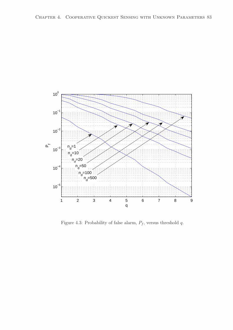
Chapter 4. Cooperative Quickest Sensing with Unknown Parameters 83
1 2 3 4 5 6 7 8 9
10−5
10−4
10−3
10−2
10−1
100
q
Pf
nd=1
nd=10
nd=20
nd=50
nd=100n
d=500
Figure 4.3: Probability of false alarm, Pf , versus threshold q.

Chapter 4. Cooperative Quickest Sensing with Unknown Parameters 84
4.6 Chapter Summary
In this chapter, we presented a linear test approach for cooperative quickest sensing in
cognitive radios. We presented several cooperative quickest sensing schemes based on
the CUSUM algorithm and derived their test statistics under noisy and noiseless channel
scenarios. However, due to unknown parameters in the distribution of the observa-
tions, such as primary signal variance, the CUSUM-based approaches are not directly
applicable to cognitive radios. For this reason, we proposed a linear test for coopera-
tive spectrum sensing, which does not require any prior knowledge or estimation of the
primary signal or channel statistics. Unlike other proposed schemes, the linear-based
schemes do not lead to any iterative algorithm or any parameter estimation and, thus,
are much simpler and faster to implement. Furthermore, we presented a threshold set-
ting method for CUSUM-based algorithms for a target probability of false alarm. We
showed that linear-based cooperative quickest sensing schemes perform comparably to
their known-parameter counterparts, while not relying on prior knowledge or estimation
of the uncertain parameters.

Chapter 5
Throughput of Cognitive Radio
Networks
In order to investigate the efficiency of quickest sensing approach and feasibility of de-
ploying CR networks based on this approach in achieving satisfactory secondary rates
while protecting the primary user, in this chapter, we analyze the achievable throughput
by quickest-based CRs and investigate the sensing-throughput tradeoff when quickest
sensing is applied. To the best of our knowledge, this analysis for quickest sensing has
not been performed in the existing literature. By analyzing the same problem for block
sensing-based CRs, we compare the achievable throughput and efficiency of these two ap-
proaches and illustrate the superiority and practicality of the quickest sensing approach.
As CR nodes cannot perform spectrum sensing and data transmission simultaneously
in the same band, a sense and then transmit approach must be applied [43–45]. Therefore
the basic frame structure used by CR networks consists of a sensing interval and a
transmission interval. Such a frame structure leads to a fundamental tradeoff [43] between
the throughput achievable by the CRs and the quality of sensing. The latter relates
directly to the level of protection for the primary user (PU). This tradeoff is due to the
following:
85

Chapter 5. Throughput of Cognitive Radio Networks 86
• Higher-quality sensing requires longer sensing times;
• For a fixed frame duration, a longer sensing time results in a shorter transmission
time for the CR and hence a lower achievable throughput.
In [43], the block sensing duration was designed to maximize CR throughput with
a given frame duration, while protecting the primary user by keeping the probability of
detection higher than a certain threshold. The similar problem of optimizing the frame
duration for a given sensing time has been considered in [44, 45]. In [44], the objective
of the optimization was to maximize the CRs throughput while keeping the probability
of collision with the primary user below a certain threshold, assuming that primary user
activity in successive frames are independent of each other. In [45], the throughput of
the CR was maximized while ensuring that the primary interference time ratio (PITR)
is less than a certain threshold. Unlike [44], it assumed dependent primary user signals
in successive frames by modeling the primary user activity as a continuous time Markov
process. Both [44] and [45] assume perfect error-free block sensing which is not realistic
and they neglect the effect of interference from the primary user on the CRs throughput.
While the existing research on throughput-sensing trade-off is focused on block sens-
ing, it is clear at least at an intuitive level that the class of quickest (sequential) sensing
schemes [29–31, 37, 60] can perform better than block-based sensing, given that the ob-
jective here is to minimize the delay between the occurrence of the event of interest
and its detection. A comparison between block and sequential sensing CR networks is
therefore investigated in this chapter. We are interested particularly in bursty primary
applications, where the question of feasibility of providing cognitive radios with a cer-
tain throughput and primary users with a certain protection level has not been studied
rigorously.
In this chapter, we derive the average throughput for both sequential and block sens-
ing, given the probability distribution of the primary network’s active and inactive peri-
ods, and assuming the CR network’s throughput is lower in the event of collision with the
Chapter 5. Throughput of Cognitive Radio Networks 87
primary user. The sequential sensing method is the Page’s cumulative sum (CUSUM)
algorithm [33,34] while the block sensing method is the energy detector. We consider two
optimization problems: one with the probability of collision as the primary user protec-
tion metric and the other with the PITR as the constraint. Unlike [44,45] we realistically
assume block sensing schemes with detection error and take into account the degradation
of CR throughput in the event of collision between the CR and primary user signals. We
solve the two optimization problems for quickest sensing and block sensing-based CRs.
Our simulation results reveal that quickest sensing results in higher average throughput
compared to block sensing, while requiring smaller frame duration and sensing time,
when the interference to the primary user is constrained to be small (as it should be
in practice). This shows quantitatively the superiority of quickest sensing compared to
block sensing in CR networks. This chapter is partially published in [65].
The remainder of this chapter is organized as follows. The system model and problem
formulation are described in Section 5.1. The derivation of the throughput, probability of
collision and PITR is presented in Section 5.2 for both quickest and block-based sensing
schemes. The solutions to the optimization problems are provided in Section 5.3. The
simulation results are presented in Section 5.4. Finally, Section 5.5 concludes the chapter.
5.1 System Model and Problem Formulation
5.1.1 System Description
We assume the primary user has a continuous-time Markov process traffic model with
the two states “on” and “off”. The on and off times are exponentially distributed with
parameters β and α respectively. This model has been assumed in previous studies [44,45,
66,67]. Sensing and transmission cannot be performed by the CR network simultaneously
in the same band. Therefore, the CR network applies a sense-then-transmit strategy

Chapter 5. Throughput of Cognitive Radio Networks 88
T X S
T0
Figure 5.1: A CR frame, showing the sensing interval in black and the data transmission
phase in a lighter shade. The primary user is inactive at the start of the frame (defined
as event H0 in the text), and comes on at time T +X from the start of the frame, leading
to collision over a duration S = T0 − T − X.
[43–45], where each frame consists of sensing and transmission phases, as depicted by the
dark and light areas in Figure 5.1. The sensing duration is T , which is random in quickest
sensing; the total frame duration is T0. If the primary user is inactive and the detector
correctly senses that state then only the CR uses the spectrum over the duration X after
sensing, and the primary user comes on for a period S while the CR is still transmitting.
X and S are random variables whether in block or sequential sensing since the primary
network has random on and off times. Clearly, T0 = T + X + S.
5.1.2 Problem Formulation
Using the above notation, we can explain the fundamental problem as follows: to max-
imize throughput for the CR without constraining interference to the primary user, we
should maximize the fraction of time the CR is transmitting, i.e. (T0 − T )/T0, but to
reduce interference to the primary user, we should increase the sensing time T so as to
improve sensing accuracy and reduce the probability of the CR and primary user trans-
missions colliding. For a given T0, the former requirement calls for small sensing time T ,
but the latter calls for large T – there is thus an optimal T that balances both require-

Chapter 5. Throughput of Cognitive Radio Networks 89
ments. Alternatively, if we consider T (or its distribution in the case of quickest sensing)
to be fixed, then increasing T0 leads to higher CR throughput but larger interference to
the primary user since S increases, so an optimal T0 exists. In this chapter, we tackle
the latter problem.
Specifically, the optimal frame duration may be found by solving this optimization
problem:
T opt0 = arg max
T0
R(T0)
s.t. Pc ≤ Pmaxc (5.1)
where R(T0) is the average throughput of the CR network as a function of T0, and Pmaxc
is the maximum probability of collision that the primary user can tolerate. This tradeoff
can also be formulated with the primary interference time ratio (PITR) as the constraint,
i.e.
T opt0 = arg max
T0
R(T0)
s.t. IR ≤ ImaxR (5.2)
where ImaxR is the maximum PITR, defined as the ratio of the average interference time
experienced by primary user to the average transmission time of the primary user. The
PITR has been used in [44, 45] as a measure of the effect of collision on the primary
user. The rate R(T0) is a function not just of T0, but also α, β, and the performance of
the sensor in terms of probabilities of false alarm and detection, as we show in the next
section.
5.1.3 CUSUM algorithm
We apply the well-known Page’s CUSUM algorithm [33] as the quickest sensing engine.
Assuming a zero-mean Gaussian primary user signal with variance σ2s and AWGN noise

Chapter 5. Throughput of Cognitive Radio Networks 90
with variance σ2n, the log likelihood ratio (LLR) based on observation z[m] is derived as
l(z[m]) =σ2
sz2[m]
2(σ2s + σ2
n)+
1
2ln
(
σ2n
σ2s + σ2
n
)
(5.3)
This LLR is accumulated in the CUSUM algorithm to form the test statistic, which is
compared against a set threshold, as explained below, to decide if the primary user is
active or inactive.
As the CUSUM algorithms for detecting a rising edge (primary user active) and a
falling edge (primary user silent) are different and we are interested in both events, we
need to run both algorithms in parallel. The rising edge detector compares the test
statistic against threshold h0, whereas the falling edge detector applies h1 as its CUSUM
threshold. The first of the two algorithms to return a positive test result will yield the
decision on primary user activity. The algorithms are as follows:
The rising edge detector [64]
1. Set g0 = 0, m = 1
2. If gm−1 < h0
• Set gm = max{0, gm−1 + l(z[m])}
• If gm = 0, set t1 = m
• If gm < h0, set m = m + 1 and goto 2)
3. If gm ≥ h0,
• A rising edge of the signal has been detected.
• t1 = m
The falling edge detector [64]
1. Set g0 = h0 + h1, m = 1

Chapter 5. Throughput of Cognitive Radio Networks 91
2. If gm−1 ≥ h0
• Set gm = min{h0 + h1, gm−1 + l(z[m])}
• If gm = h0 + h1, set t2 = m
• If gm > h0, set m = m + 1 and goto 2)
3. If gm ≤ h0,
• A falling edge of the signal has been detected.
• t2 = m
In the pseudo-codes above, t1 and t2 are respectively the times at which a positive
result is returned by the rising and falling edge detectors. If t1 ≤ t2 the algorithm declares
that the primary user is active and otherwise declares the availability of the band. A key
observation from simulations is that the probability that t2 > t1 when the primary user
is idle is negligible, and so is the probability that t1 > t2 when the primary user signal
is on. Therefore, we assume that our proposed parallel CUSUM rising and falling edge
detection algorithm always correctly detects the activity of the primary user.
5.2 Derivation of R(T0), Pc and IR
In this section, we derive expressions for the three quantities in (5.1) and (5.2) for both
quickest sensing and block sensing, so that the optimization problems can be rigorously
formulated and then solved.
5.2.1 Quickest Spectrum Sensing
Preliminaries
The primary user is either active or inactive at the start of a CR frame. In both of these
scenarios we assume that the primary user’s activity state remains unchanged during the
Chapter 5. Throughput of Cognitive Radio Networks 92
sensing interval. This implies that the expected on and off durations of the primary user
are much larger than the expected sensing time. This assumption was made in related
previous studies [43–45].
In quickest sensing, the CR is assumed to detect the activity of the primary user
correctly with probability one, as mentioned in the previous section. Therefore, when
the primary user is active at the beginning of the CR frame, quickest sensing detects
this activity after sensing time T , and refrains from transmission in that frame. In that
case, the throughput of the CR is zero. When the primary user is idle, on the other
hand, the CR starts transmission after sensing time T . However, the primary user may
resume transmission during the CRs transmission phase, which results in collision. This
collision degrades the throughput of the CR. Unlike most studies where the interference
from the primary user to the CR has been neglected [44,45], we take into account the rate
degradation to the CR due to collision. We denote the throughput of the CR network
with no collision as C0 and the throughput with collision as C1. For instance, in a point-
to-point transmission in the CR network with SNR of SNRc and interference SNR from
the primary user to the CR of SNRp and Gaussian primary user and CR signals, we have
C0 = log2(1 + SNRc) and C1 = log2(1 + SNRc
1+SNRp). It is clear that C0 > C1.
Referring to Figure 5.1, let V = X + T . Also, we denote by H0 the event that the
primary network is not active at the start of the frame, and by H1 its complement. The
achievable rate is then
R(T0) = P (H0)R0(T0) + P (H1)R1(T0) (5.4)
where Ri(T0) is the rate conditioned on Hi, and P (Hi) is the probability of Hi. Since
the probability of missed detection (detection error) is negligible in the proposed quickest
sensing scheme, R1(T0) = 0. Therefore we have that
R(T0) = P (H0)R0(T0) (5.5)
When the primary user is inactive at the start of the frame, there are three scenarios

Chapter 5. Throughput of Cognitive Radio Networks 93
to consider:
1. T ≤ T0, V ≤ T0: The CR transmits at the rate C0 for time X = V − T , and at the
rate C1 for the remaining time T0 − V ;
2. T ≤ T0, V > T0: The primary user does not return until after the end of the frame,
so the CR transmits at the rate C0 for the duration T0 − T ;
3. T > T0: The CR takes so long to detect the availability of the band that the
transmission opportunity is lost for that frame. The rate is 0.
Exact Expressions
With the above breakdown, we have
RQ(T0) =
[
P (V ≤ T0)
{
E
[
X
T0
∣
∣
∣
∣
V ≤ T0
]
C0 + E
[
T0 − V
T0
∣
∣
∣
∣
V ≤ T0
]
C1
}
+P (V > T0, T ≤ T0)
{
E
[
T0 − T
T0
∣
∣
∣
∣
V > T0, T ≤ T0
]
C0
}]
P (H0) (5.6)
Thus the achievable rate depends on the distributions of the random variables X, T and
V , which we will now derive.
As mentioned before, the idle time is exponentially distributed with parameter α,
thus the probability density function (pdf) of X is
fX(x) = αe−αx, x ≥ 0. (5.7)
(Recall that the exponential distribution has the memory-less property P [T > t1+t2|T >
t2] = P [T > t1], and so even though the start of the transmission phase in the CR
frame does not coincide with the instant the channel becomes idle, the same exponential
distribution applies.) The sensing time T in the CUSUM algorithm is a random variable
whose exact distribution is not known. For simplicity, we model T as an exponential
random variable with parameter λ. Our simulation results (in Section 5.4) verify this
assumption.

Chapter 5. Throughput of Cognitive Radio Networks 94
Given that the primary user idle time is exponential with parameter α and its active
time is exponential with parameter β, the prior probabilities of primary user activity at
the start of each CR frame are
P (H0) =β
α + βand (5.8)
P (H1) =α
α + β. (5.9)
In order to derive an expression for the average throughput in (5.5), first we need to
determine the joint pdf of X and T . As the sensing time of the CR and the idle time of
the primary user are independent exponential random variables we have
fX,T (x, t) =
{
αe−αxλe−λt, x ≥ 0, t ≥ 0
0 otherwise.(5.10)
Through straightforward integration of fX,T (x, t) over the appropriate regions in the x-t
plane, we derive the probability terms in (5.6) as
P (V ≤ T0) = 1 +α
λ − αe−λT0 − λ
λ − αe−αT0 (5.11)
and
P (V > T0, T ≤ T0) =λ
λ − α
(
e−αT0 − e−λT0)
. (5.12)
To evaluate the expected value terms in (5.6), we first find the conditional distri-
butions of X and T conditioned on {V ≤ T0} and {V > T0, T ≤ T0}, as outlined in
Appendix C. Then we obtain
E
[
X
T0
∣
∣
∣
∣
V ≤ T0
]
= 1−1 − 1−e−αT0
T0α− αe−λT0
α−λ+ αe−λT0−αe−αT0
T0(α−λ)2
1 + αλ−α
e−λT0 − λλ−α
e−αT0
(5.13)
E
[
T
T0
∣
∣
∣
∣
V ≤ T0
]
= 1−1 − 1−e−λT0
T0λ− λe−αT0
λ−α+ λe−αT0−λe−λT0
T0(λ−α)2
1 + αλ−α
e−λT0 − λλ−α
e−αT0
(5.14)

Chapter 5. Throughput of Cognitive Radio Networks 95
E
[
T0 − T
T0
∣
∣
∣
∣
V >T0, T ≤T0
]
=
1λ−α
(
e−λT0
T0− e−αT0
T0
)
+ e−αT0
e−αT0 − e−λT0.
(5.15)
Consequently, the average CR throughput is derived as
RQ(T0) =
[
(αe−λT0−λe−αT0)
(
C1
λ − α
)
+1
T0
(
C0
α−C1
λ + α
λα
)
+e−λT0
T0
(
C0 − C1
λ − α+
C1(λ + α)
λα− C0
α
)
+e−αT0
T0
(
C1 − C0
λ − α
)
+C1
]
P (H0)(5.16)
Even if the primary user is idle during the sensing period, it may become active during
the transmission period and collide with the CR. The interference to the primary user
can be evaluated by the probability of collision which is defined as
PcQ= P (H0)P (V ≤ T0) (5.17)
or by the PITR which is the ratio of the average collision time to the average activity
time of primary user, defined as
IRQ=
P (H0)E[S]
β−1. (5.18)
These definitions are based on the assumptions that the CR network has full traffic and
once the primary user becomes active it remains busy until the end of the frame. The
latter assumption is realistic when the average primary user active time is larger than
the frame duration. Using (5.8) and (5.11) in (5.17), we will obtain the probability of
collision, so the only remaining problem is finding IRQ, which requires E[S], derived as
follows:
E[S] = P (H0)E[T0 − V |V ≤ T0]P (V ≤ T0) (5.19)
= P (H0)[T0P (V ≤T0)−E[V |V ≤ T0]P (V ≤T0)] (5.20)
To find E[V |V ≤ T0] = E[X +T |V ≤ T0], we can apply the derived expressions in (5.13)
and (5.14). Furthermore, by substituting (5.11) into (5.20), IRQis derived as
IRQ= P (H0)
(
T0β+β
λ − α
[
λ
α(1 − e−αT0)−α
λ(1 − e−λT0)
])
.
(5.21)

Chapter 5. Throughput of Cognitive Radio Networks 96
5.2.2 Block-Based Sensing
Preliminaries
Block sensing schemes have a non-negligible probability of making decision errors. This
fact, together with the non-random nature of the sensing interval T , changes the analysis
compared to the quickest sensing case of the last section.
In block-based sensing schemes, based on the activity state of the primary user at
the beginning of the frame, two scenarios may occur. The first scenario is that the
primary user is idle when the CR frame starts and it can potentially become active
during the transmission slot of the primary user. In this case, unlike in the quickest
sensing framework, the primary user can be falsely detected to be active (false alarm)
and the CR would miss the transmission opportunity. The second scenario happens when
the primary user is active during the sensing slot and can potentially become idle in the
transmission slot. In this case, the activity of the primary user could be falsely detected
as being idle (missed detection) by the block-based sensing scheme. In this case, the
CR would start transmission after the sensing slot and would cause collision with the
primary user. This collision lasts as long as the primary user is active during the frame.
In order to analyze the CR throughput under H1, we denote the active time of the
primary user by Y , which based on the exponential model for the active duration of the
primary user, has pdf
fY (y) = βe−βy, y ≥ 0. (5.22)
Under H1, this variable replaces random variable X in Figure 5.1. We define random
variable W = Y + T under H1. Also, we define the probabilities of false alarm and
detection respectively as Pf = P (θ̂ = 1|H0) and Pd = P (θ̂ = 1|H1), where θ̂ denotes the
sensing result of the block-based sensing scheme.
For N -sample energy detection as the block sensing scheme, decision making is as

Chapter 5. Throughput of Cognitive Radio Networks 97
follows:
u =
{
1 ,∑N
m=1 z[m]2 ≥ ǫ
0 ,∑N
m=1 z[m]2 < ǫ,(5.23)
where ǫ is the energy threshold. The energy threshold is chosen to maintain a certain
local probability of false alarm Pf . The probabilities of false alarm and detection for
energy detection are determined as [16]
Pf = Q
(
ǫ − Tfsσ2n√
2Tfsσ2n
)
(5.24)
Pd = Q
(
ǫ − Tfs(σ2s + σ2
n)√2Tfs(σ2
s + σ2n)
)
(5.25)
where Q(·) is the inverse Q-function, ǫ is the threshold, T is the sensing time, fs is the
sampling frequency and σ2n and σ2
s are respectively the noise and signal power.
Exact Expressions
When the primary user is inactive at the start of the frame, the CR detects this oppor-
tunity with probability 1 − Pf . In this case, there are three scenarios to be considered
which are identical to the ones described for quickest sensing and will not be repeated
here. On the other hand, under H1, block-based sensing could falsely declare that the
primary user is inactive with probability 1−Pd and the CR starts transmission while the
primary user signal is on. In this case, there are two scenarios to consider:
1. W ≤ T0: The CR transmits at the rate C1 for time Y = W − T , and at the rate
C0 for the remaining time T0 − W ;
2. W > T0: The primary user remains active until after the end of the frame, so the
CR transmits at the rate C1 for the duration T0 − T ;

Chapter 5. Throughput of Cognitive Radio Networks 98
With the above description, we derive the average throughput for CR with block-
based sensing as follows
RB(T0) = P (H0)(1 − Pf)
{
P c0
(
C0E
[
X
T0
∣
∣
∣
∣
X < T0 − T
]
+C1E
[
T0 − V
T0
∣
∣
∣
∣
X + T < T0
]
)
+ C0(1 − P c0 )
(
T0−T
T0
)
}
+P (H1)(1 − Pd)
{
P c1
(
C1E
[
Y
T0
∣
∣
∣
∣
Y < T0 − T
]
+C0E
[
T0 − W
T0
∣
∣
∣
∣
Y < T0 − T
]
)
+ C1(1 − P c1 )
(
T0 − T
T0
)
}
(5.26)
where P c0 = P (X < T0 − T ) and P c
1 = P (Y < T0 − T ). To calculate the average
throughput achievable by a block-based sensing CR network, we derive the expected
values and probabilities in (5.26) as follows:
E
[
X
T0
∣
∣
∣
∣
V ≤ T0
]
= 1 − T
T0−
1 − TT0
− 1−e−α(T0−T )
αT0
1 − e−α(T−T0)(5.27)
E
[
Y
T0
∣
∣
∣
∣
W ≤ T0
]
= 1 − T
T0−
1 − TT0
− 1−e−β(T0−T )
βT0
1 − e−β(T−T0)(5.28)
P c0 = 1 − e−α(T0−T ) (5.29)
P c1 = 1 − e−β(T0−T ) (5.30)
Consequently, the average throughput of a CR network with block-based sensing is
derived as
RB(T0) = P (H0)(1 − Pf)
[
C1 +1
T0
(
C0 − C1
α− TC1
)
+e−α(T0−T )
T0
(
C1 − C0
α
)
]
+ P (H1)(1 − Pd)
×[
C0 +1
T0
(
C1 − C0
α− TC0
)
+e−β(T0−T )
T0
(
C0 − C1
β
)
]
(5.31)

Chapter 5. Throughput of Cognitive Radio Networks 99
In finding the probability of collision, we should note that in block sensing CRs, there
is a non-zero probability of collision under both H0 and H1 as described before and thus
Pc can be written as
PcB= P (H0)(1 − Pf)P
c0 + P (H1)(1 − Pd) (5.32)
= P (H0)(1 − Pf)(1 − e−α(T0−T ))+P (H1)(1 − Pd) (5.33)
The PITR is derived as
IRB=
P (H0)E[S|H0] + P (H1)E[S|H1]
β−1
= β (P (H0)E[T0 − T − X] + P (H1)E[T0 − T − Y ]) .
= β(T0 − T ) +β
αP (H0)
(
1 − e−α(T0−T ))
+ P (H1)(
1 − e−β(To−T ))
.
(5.34)
5.3 Solving the Optimization Problem
5.3.1 Quickest Sensing
Using the expressions derived for the average CR throughput and the probability of
collision respectively in (5.16) and (5.11), the optimization problem (5.1) can be expressed
as
T opt0Q
= arg maxT0
RQ(T0)
s.t. P (H0)
(
1 +α
λ − αe−λT0− λ
λ − αe−αT0
)
≤PmaxcQ
(5.35)
In order to check the existence of an optimal solution we first examine the first derivative
of RQ(T0):
dRQ(T0)
dT0=
[
(e−αT0 − e−λT0)
(
αλC1
λ − α
)
− 1
T 20
(
C0
α− C1
λ + α
λα
)
−(λT0 + 1)e−λT0
T0
(
C0 − C1
λ − α+
C1(λ + α)
λα− C0
α
)
−(αT0 + 1)e−αT0
T0
(
C1 − C0
λ − α
)
+ C1
]
P (H0) (5.36)

Chapter 5. Throughput of Cognitive Radio Networks 100
As we show in the next section, whether any T0 drives the derivative above to zero
depends on λ and C1/C0. Intuitively, as the frame duration increases, the average rate
eventually converges to P (H0)C1 since the probability of the primary user returning to
the channel approaches 1 and the collision interval S approaches T0−T ≈ T0. Conversely
as T0 shrinks, the rate goes to zero since both terms in RQ(T0) disappear.
Considering the constraint in (5.35), the probability of collision PcQis a monotonically
increasing function of the frame duration as its first derivative,
dPcQ
dT0
= P (H0)αλ
λ − α(e−αT0 − e−λT0), (5.37)
is a positive function of T0. Hence, we must have
T0 ≤ P−1cQ
(PmaxcQ
) (5.38)
where P−1cQ
(·) is the inverse function of PcQ(·) in (5.17). Therefore, the probability of col-
lision imposes an upper bound on the frame length. If RQ(T0) does not have a maximum
in the range (5.38), the optimal T0 is this upper bound; otherwise the optimal T0 is the
stationary point of RQ(T0) found by setting (5.36) to zero.
Considering the optimization problem in (5.2) and using the derived expression for
the throughput and PITR in (5.16) and (5.21) we get
T opt0Q
= arg maxT
RQ(T0)
s.t. P (H0)
[
T0β +β
λ − α
(
λ
α(1 − e−αT0)−α
λ(1−e−λT )
)]
≤ ImaxRQ
.
(5.39)
By taking the derivative of IRQ,
dIRQ
dT0= P (H0)
[
β +β
λ − α(λe−αT0 − αe−λT0)
]
, (5.40)
we observe that the PITR monotonically increases with T0 as its derivative is a positive
function of T . Therefore, for a certain threshold ImaxRQ
the optimal frame duration is
bounded by
T opt0Q
≤ I−1RQ
(ImaxRQ
) (5.41)

Chapter 5. Throughput of Cognitive Radio Networks 101
where I−1RQ
(·) is the inverse function of IRQ(·) in (5.21).
Again, the optimal T0 is the right-hand side of (5.41) if there is no stationary point
of RQ(T0) in the range (5.41), otherwise it will be the value that drives (5.36) to zero.
5.3.2 Block-Based Sensing
The optimization problem (5.1) for block-based sensing schemes can be written as
T opt0B
= arg maxT0
RB(T0)
s.t.P (H0)(1−Pf)(1−e−α(T0−T ))+P (H1)(1−Pd)≤PmaxcB
(5.42)
where RB(T0) is derived in (5.31). By examining the first derivative of RB(T0) as below
dRB(T0)
dT0= P (H0)(1 − Pf)
[
− 1
T 20
(
C0 − C1
α− TC1
)
−(αT0 + 1)e−α(T0−T )
T 20
(
C1 − C0
α
)
]
+ P (H1)(1 − Pd)
×[
− 1
T 20
(
C1 − C0
α− TC0
)
− (βT0 + 1)e−β(T0−T )
T 20
(
C0 − C1
β
)
]
.
(5.43)
We observe that depending on the values of C1/C0 and T the rate function (5.31) po-
tentially has a local maximum. We also investigate the behavior of the probability of
collision by deriving its first derivative with respect to the frame duration,
dPcB
dT0= P (H0)(1 − Pf )αe−α(T0−T ). (5.44)
This derivative is a positive function of T0, and hence, the probability of collision
monotonically increases with the frame duration. Therefore, in this optimization prob-
lem, the optimal frame length is upper-bounded as
T opt0B
≤ P−1cB
(PmaxcB
) (5.45)
where P−1cB
(·) is the inverse function of PcB(·) in (5.33). As we show in the next section,
based on the value of C1/C0, the average rate function of the block-based sensing CR

Chapter 5. Throughput of Cognitive Radio Networks 102
either has a local maximum or is monotonically increasing with the frame length and
it eventually converges to P (H0)(1 − Pf)C1 + P (H1)(1 − Pd)C0 as T0 grows large. In
the latter case, the optimal frame length is the bound in (5.45), whereas in the former
case the optimal frame length is determined in a similar fashion as the quickest sensing
scenario in Section 5.3.1.
Considering the optimization problem (5.2) for block sensing-based CRs results in
similar solutions to the ones for quickest sensing, as again the first derivative of the
PITR,
dIRB
dT= β + βP (H0)e
−α(T0−T ) + βP (H1)e−β(T0−T ) (5.46)
is a nonnegative function of the frame length. Thus we observe that the PITR mono-
tonically increases with T0 and for a certain threshold ImaxRB
the optimal frame duration
must satisfy
T opt0B
≤ I−1RB
(ImaxRB
) (5.47)
where I−1RB
(·) is the inverse function of IRB(·) in (5.34). If the maximum is achieved at a
lower frame length than the upper bound in (5.47), then the optimal frame length is the
first zero of (5.43). Otherwise, the optimal frame length is
T opt0B
= I−1RB
(ImaxRB
). (5.48)
5.4 Simulation Results
Consider a single CR network and a single primary user. We choose the activity parame-
ters of the primary user according to VoIP traffic [44,45] where the mean idle and active
durations of the primary user are respectively α−1 = 650 ms and β−1 = 352 ms. The
sampling rate is fs = 1000 Hz and the CR transmits one packet per slot. The primary
user signal variance σ2s and AWGN noise variance σ2
n are assumed to be 1.
Fig. 5.2 shows the normalized average throughput RQ/C0, and probability of collision
PcQ, of the quickest sensing-based CR network versus the frame duration. The average

Chapter 5. Throughput of Cognitive Radio Networks 103
0 0.5 1 1.5 20
0.1
0.2
0.3
0.4
0.5
0.6
0.7
Frame length, T0
Ave
rage
thro
ughp
ut/C
0
RQ
/C0, Theoretical
RQ
/C0, Simulated
C1/C
0=0.5C
1/C
0=0.8
Pc
Figure 5.2: Average normalized throughput, RQ/C0, and probability of collision, PcQ,
versus frame duration T0 for quickest sensing.
sensing time is λ−1 = 7.2 ms. We observe that the simulated average throughput is
very close to the theoretical one derived in (5.16). This verifies the suitability of the
exponential assumption for the distribution of the quickest sensing time in the average
throughput analysis. We also observe that depending on C1/C0 the average rate may
have a local maximum. The probability of collision, on the other hand, is a monotonically
increasing function of frame duration. We observe that for acceptable levels of collision
probability (e.g., below 0.1) the frame length is small and falls in the monotonically
increasing part of the average rate function. Therefore the optimal frame length is directly
determined by the constraint on the probability of collision as in (5.38).
Fig. 5.3 shows the normalized average throughput RQ/C0, and primary interference
time ratio (PITR), IRQ, of the quickest sensing-based CR network versus the frame
duration. The average sensing time is λ−1 = 7.2 ms. We observe that the PITR is a
monotonically increasing function of frame duration. Depending on the acceptable levels

Chapter 5. Throughput of Cognitive Radio Networks 104
0 0.5 1 1.5 20
0.5
1
1.5
2
2.5
Frame length, T0(s)
Ave
rage
thro
ughp
ut/C
0
RQ
/C0, Theoretical
RQ
/C0, Simulated
C1/C
0=0.5
C1/C
0=0.8I
RQ
Figure 5.3: Average normalized throughput, RQ/C0, and primary interference time ratio
(PITR), IRQ, versus frame duration T0 for quickest sensing.
of PITR the optimal frame length may fall in the monotonically increasing part of the
average rate function or to the right of its peak point. Therefore in the latter case, the
optimal T0 in the optimization problem (5.39) is the stationary point of RQ(T0) found
by setting (5.36) to zero, whereas in the former case the optimal T0 is the upper bound
imposed by the PITR constraint in (5.41).
Fig. 5.4 shows the average throughput of quickest sensing-based CR network as
well as block sensing-based CR network versus probability of collision. The points of
these curves are achieved by changing the frame duration T0. The block sensing scheme
considered is energy detection. For block sensing CR we consider two cases. In case 1,
the sensing time of the block sensing is set to be the same as the average sensing time of
the quickest sensing, T = λ−1 = 7.2 ms and the probabilities of false alarm and detection
are respectively Pf = 0.15 and Pd = 0.8. In case 2 the probabilities of false alarm and
detection are set to be respectively Pf = 0.05 and Pd = 0.9 which requires a longer sensing

Chapter 5. Throughput of Cognitive Radio Networks 105
0 0.1 0.2 0.3 0.4 0.50
0.1
0.2
0.3
0.4
0.5
0.6
Probability of collision
Ave
rage
thro
ughp
ut/C
0
Quickest sensingBlock sensing, case2Block sensing, case1
C1/C
0=0.8
C1/C
0=0.5
C1/C
0=0.1
Figure 5.4: Average normalized CR throughput, versus probability of collision.
time of T = 17.7 ms. We observe that the probability of collision in block sensing has a
lower bound and cannot be reduced further due to its fixed sensing time. For example in
case 1, where the block sensing time is the same as the average quickest sensing time, the
probability of collision for block sensing cannot be lower than 0.07 whereas the probability
of collision in quickest sensing can be lowered as much as desired. For the probability
of collision of 0.05, the average throughput for the quickest sensing-based CR is 0.56
whereas the average throughput of the block sensing-based CR is 0.29 in case 2, where
the block sensing time is more than two times of the average quickest sensing time. For
the probability of collision of 0.08, the average throughput for the quickest sensing-based
CR is 0.59 (for C1/C0 = 0.8) whereas the average throughput of the block sensing-based
CR in case 1 (with the same sensing time as the quickest sensing) is 0.37. We observe
that for the same probability of collision, the quickest sensing-based CR achieves a much
higher average throughput compared to the block sensing-based CR even when the block
sensing time is much larger than the average quickest sensing time.

Chapter 5. Throughput of Cognitive Radio Networks 106
0 0.1 0.2 0.3 0.4 0.5 0.60
0.1
0.2
0.3
0.4
0.5
0.6
Ave
rage
thro
ughp
ut/C
0
Probability of collision
Quickest sensingBlock sensing, case2Block sensing, case1
Figure 5.5: Average normalized CR throughput, versus probability of collision.
Fig. 5.5 depicts the average throughput of quickest sensing-based CR network as
well as block sensing-based CR network versus probability of collision for the case of
C1/C0 = 0.1. We can observe that the average throughput in the quickest sensing scenario
goes as low as 0.068 as the probability of collision converges to 0.64. This totally complies
with the analytical statement in Section 5.3.1 that the average normalized throughput
in the quickest sensing scenario converges to P (H0)C1/C0 as the block length increases
and the probability of collision converges to P (H0). For the block sensing scenario, the
average normalized throughput converges to P (H0)(1 − Pf )C1/C0 + P (H1)(1 − Pd) and
the probability of collision converges to P (H0)(1−Pf)+P (H1)(1−Pd) as the block length
grows. This is verified by this figure where in the case 2 scenario, for example, the average
normalized throughput converges to 0.09 as the probability of collision goes to 0.65. Once
again, we observe that for acceptable values of the probability of collision (e.g., below
0.2), the quickest sensing achieves much higher average throughput compared to the
block sensing scheme. For instance, for the probability of collision of 0.04, the quickest

Chapter 5. Throughput of Cognitive Radio Networks 107
sensing achieves average normalized throughput of 0.53 whereas the average normalized
throughput of the block sensing-based CR in case 2 is 0.015.
5.5 Chapter Summary
In this chapter, we studied the optimization of the frame duration of quickest sensing-
based and block sensing-based cognitive radios (CRs), to achieve the maximum CR
throughput while protecting the primary user by keeping the collision probability or
PITR (primary interfered time ratio) below a certain threshold. Analytical expressions
for the average throughput, probability of collision and PITR for both quickest and block-
based sensing approaches were found. These expressions were used to find the optimal
frame duration for a certain quality of service for the primary user and the CR with both
sensing approaches. We compared the maximum average throughput in block-based
and quickest sensing schemes and showed that the quickest sensing approach results in
a considerably higher CR throughput while requiring shorter frame length and sensing
time at realistically low primary interference levels. These results show the superiority
of quickest sensing approach compared to the conventional block sensing approach in
cognitive radio networks.

Chapter 6
Conclusion
6.1 Summary of Conclusions
The increasing demand for wireless services and the static spectrum allocation policies
have led to spectrum scarcity in wireless communications. On the other hand, studies
show that most of the radio frequency spectrum is under-utilized [3]. This is mainly due
to the spectrum allocation policies that traditionally have fixed assignment of frequency
resources to licensed or primary users. These policies do not allow unlicensed or secondary
users to utilize rarely used allocated frequencies, even when no interference with the
assigned service would occur.
Recently, cognitive radios (CRs) have been introduced as a potential solution to this
problem [5, 6]. In a widely studied form of CR technology sometimes known as oppor-
tunistic or dynamic spectrum access, the secondary users, are allowed to opportunistically
utilize a frequency band allocated to primary users, when it is not being used. The CR
network has to be able to detect the presence of the primary network’s signals, so as to
avoid interfering with it. Therefore, spectrum sensing plays a crucial role in the successful
deployment of CRs.
In Chapter 2, we presented a probabilistic inference approach for cooperative spec-
108

Chapter 6. Conclusion 109
trum sensing. This approach allows for modeling and accommodating the uncertainties
and correlations in the cooperative sensing system and applying belief propagation for
inferring the likelihood functions. We derived the NP-based LRT at the FC for hard, soft
and quantized local decisions. Unlike most existing studies, we consider the presence of
fading and noise in the transmission channels.
Due to lack of primary signal and channel knowledge in cognitive radios, most exist-
ing results in the distributed detection literature which assume known transmit signals,
cannot be directly applied to the cooperative sensing problem. Therefore, in Chapter 3
we proposed a linear composite hypothesis testing approach which does not require any
prior knowledge or estimates of the unknown parameters and performs very closely to
the known-parameter optimal LRT.
We also studied quickest change detection for spectrum sensing in cognitive radios in
Chapter 4. Presenting several cooperative quickest sensing approaches in cognitive radios,
we derived the optimal CUSUM test statistics in each scenario. To tackle the problem
of unknown primary signal and channel statistics in cognitive radios, we proposed linear
test-based CUSUM algorithms, which unlike the existing procedures, do not require any
parameter estimation or iterative algorithms.
We formulated and studied the sensing-throughput trade-off of the quickest sensing
approach in Chapter 5. We maximized the throughput of a cognitive radio network with
respect to the frame length when quickest sensing is used. The amount of interference
to the primary network, measured by the probability of collision with primary users
or the primary interference time ratio (PITR), was constrained. The corresponding
problems when CRs use block sensing were also solved, assuming that collision with
primary users causes a drop in throughput for the CR. We then compared the maximum
achievable throughput with block and quickest sensing schemes and showed that for the
same protection level to the primary network, the quickest sensing approach results in
significantly higher average throughput. Our results revealed that the quickest sensing
Chapter 6. Conclusion 110
approach is potentially more suitable for cognitive radio technology than the conventional
block sensing approach.
6.2 Future Work
This thesis presents the probabilistic inference and graphical modeling approach for coop-
erative spectrum sensing and highlights only some of the potential for graphical modeling
and message passing useful tools. Ever since many papers inspired by our work, have
tried to apply probabilistic inference and message passing algorithms into different as-
pects of cooperative spectrum sensing [68–76]. Further investigations into the effects of
a mismatch between assumed and true distributions, correlations over time and space of
fading channels and activity pattern of the primary user can be a direction of future work.
Another interesting direction for future research is application of probabilistic inference
approach to distributed (decentralized) spectrum sensing. For instance, the spatial inter-
actions among the secondary users can be represented on a factor graph where individual
beliefs of the primary user activity can be reached through an iterative message passing
algorithm among the secondary users. Preliminary research in this direction has been
presented in [70].
The unknown parameter scheme proposed in Chapter 3, can be applied to many
other unknown-parameter sensing scenarios that may arise in cognitive radio networks.
In particular, a future research direction can be towards applying the proposed approach
to distributed spectrum sensing problems with unknown parameters.
Another possible future work is applying the proposed sensing approaches in a femto-
cell network framework. The quickest sensing approach seems appropriate for femtocells
as the primary users are mainly cellular networks. Developing suitable cooperative quick-
est sensing schemes for cognitive femtocells can be an interesting future work.
The throughput analysis presented in Chapter 5 was the first step towards throughput-

Chapter 6. Conclusion 111
sensing tradeoff analysis for CR networks with quickest sensing. This topic can be further
investigated and extended to cooperative quickest spectrum sensing as a future research
direction. This extension should accommodate the spectrum sharing algorithms and
multiple-access protocols developed for multi-user cognitive radio networks.

Bibliography
[1] D. Cabric, S. M. Mishra, and R. W. Brodersen, “Implementation issues in spectrum
sensing for cognitive radios,” Proc. 38th. Asilomar Conference on Signals, Systems,
and Computers, pp. 772–776, 2004.
[2] V. Chandrasekhar, J. G. Andrews, and A. Gatherer, “Femtocell networks: a survey,”
IEEE Communications Magazine, vol. 46, pp. 59–67, Sept. 2008.
[3] “Spectrum policy task force report, FCC 02-155,” Federal Communications Com-
mission, Nov. 2002.
[4] V. Valenta, R. Marsalek, G. Baudoin, M. Villegas, M. Suarez, and F. Robert, “Sur-
vey on spectrum utilization in Europe: Measurements, analyses and observations,”
in Proc. Fifth International Conference on Cognitive Radio Oriented Wireless Net-
works and Communications (CROWNCOM), pp. 1–5, June 2010.
[5] J. Mitola and G. Q. Maguire, “Cognitive radios: making software radios more per-
sonal,” IEEE Personal Communications, vol. 6, no. 4, pp. 13–18, Aug. 1999.
[6] S. Haykin, “Cognitive radio: Brain-empowered wireless communications,” IEEE
Transactions on Information Theory, vol. 23, no. 2, pp. 201–220, Feb 2005.
[7] “Spectrum access and the promise of cognitive radio technology,” Federal Commu-
nications Commission (FCC) Cognitive Radio Technologies Proceeding (CRTP),ET
Docket No. 03-108, May 2003.
112

Bibliography 113
[8] C. Stevenson, G. Chouinard, Z. Lei, W. Hu, S. Shellhammer, and W. Caldwell,
“IEEE 802.22: The first cognitive radio wireless regional area networks (WRANs)
standards,” IEEE Communications Magazine, vol. 47, no. 1, pp. 130–138, Jan. 2009.
[9] T. Yucek and H. Arslan, “A survey of spectrum sensing algorithms for cognitive
radio applications,” IEEE Communications Surveys and Tutorials, vol. 11, no. 1,
pp. 116–130, 2009.
[10] Y. Zeng, Y.-C. Liang, A. T. Hoang, and R. Zhang, “A review on spectrum sensing
for cognitive radio: challenges and solutions,” EURASIP Journal on Advances in
Signal Processing, pp. 1–16, 2010.
[11] A. Sahai and D. Cabric, “Spectrum sensing: fundamental limits and practical chal-
lenges,” in Proc. IEEE International Symposium on New Frontiers in Dynamic Spec-
trum Access Networks (DySPAN), 2005.
[12] D. Cabric, A. Tkachenko, and R. Brodersen, “Spectrum sensing measurements of
pilot, energy, and collaborative detection,” in Proc. IEEE Military Communications
Conference, pp. 1–7, 2006.
[13] W. A. Gardner, “Exploitation of spectral redundancy in cyclostationary signals,”
IEEE Signal Processing Magazine, no. 2, pp. 14–36, 1991.
[14] S. Enserink and D. Cochran, “A cyclostationary feature detector,” in Proc. 28th
Asilomar Conference on Signals, Systems, and Computers, pp. 806–810, 1994.
[15] S. M. Kay, Optimal stopping rules, vol. 2. Prentice Hall, 1998.
[16] H. Urkowitz, “Energy detection of unkown deterministic signals,” Proc. IEEE,
vol. 55, no. 4, pp. 523–531, 1967.
[17] E. V. S. Kuffner and R. Peterson, “On collaborative detection of TV transmissions
in support of dynamic spectrum sharing,” Proc. IEEE International Symposium on
Bibliography 114
New Frontiers in Dynamic Spectrum Access Networks (DySPAN), pp. 338–345, Nov.
2005.
[18] A. Ghasemi and E. S. Sousa, “Collaborative spectrum sensing for opportusitic access
in fading enviroments,” Proc. IEEE International Symposium on New Frontiers in
Dynamic Spectrum Access Networks (DySPAN), Nov. 2005.
[19] H. Uchiyama, K. Umebayashi, Y. Kamiya, Y. Suzuki, T. Fujii, F. Ono, and K. Sak-
aguchi, “Study on cooperative sensing in cognitive radio based AD-HOC network,”
in Proc. IEEE International Symposium on Personal, Indoor and Mobile Radio Com-
munication (PIMRC), pp. 1–5, 2007.
[20] D. Cabric, A. Tkachenko, and R. W. Brodersen, “Experimental study of spectrum
sensing based on energy detection and network cooperation,” in Proc. ACM 1st
International Workshop on Technology and Policy for Accessing Spectrum (TAPAS),
2006.
[21] L. Chen, J. Wang, and S. Li, “An adaptive cooperative spectrum sensing scheme
based on the optimal data fusion rule,” in Proc. IEEE International Symposium on
Wireless Communication Systems (ISWCS), pp. 582–586, Oct. 2007.
[22] Z. Quan, S. Cui, and A. H. Sayed, “Optimal linear cooperation for spectrum sensing
in cognitive radio networks,” IEEE Journal of Selected Topics in Signal Processing,
vol. 2, no. 1, pp. 28–40, Feb. 2008.
[23] G. Ganesan and Y. Li, “Cooperative spectrum sensing in cognitive radio networks,”
Proc. IEEE International Symposium on New Frontiers in Dynamic Spectrum Access
Networks (DySPAN), pp. 137–143, 2005.
[24] S. M. Mishra, A. Sahai, and R. W. Brodersen, “Cooperative sensing among cognitive
radios,” in Proc. IEEE International Conference on Communications (ICC), 2006.

Bibliography 115
[25] G. Ganesan and Y. Li, “Agility improvement through cooperative diversity in cogni-
tive radio,” in Proc. IEEE Global Telecommunications Conference (GLOBECOM),
vol. 5, pp. 2505–2509, 2005.
[26] “Second report and order and memorandum opinion and order: In the matter of
unlicensed operation in the TV broadcast bands,” Federal Communications Com-
mission (FCC), Nov. 2008.
[27] R. Tandra and A. Salehi, “SNR walls for signal detection,” IEEE Journal on Special
Topics in Signal Processing, vol. 2, pp. 4–17, Feb. 2008.
[28] S. M. Kay, Fundamentals of Statistical Signal Processing: Estimation Theory, vol. 1.
Prentice Hall, 1998.
[29] H. V. Poor and O. Hadjiliadis, Quickest Detection. Cambridge University Press,
2008.
[30] L. Lifeng, F. Yijia, and H. V. Poor, “Quickest detection in cognitive radio: A se-
quential change detection framework,” in Proc. IEEE Global Telecommunications
Conference (GLOBECOM), pp. 1–5, 2008.
[31] H. Li, C. Li, and H. Dai, “Quickest spectrum sensing in cognitive radio,” in Proc.
Conference on Information Science and Systems, 2008.
[32] A. Jayaprakasam and V. Sharma, “Sequential detection based cooperative spec-
trum sensing algorithms in cognitive radio,” in Proc. First UK-India International
Workshop on Cognitive Wireless Systems (UKIWCWS), pp. 1–6, 2009.
[33] E. Page, “Continuous inspection schemes,” Biometrika, vol. 41, pp. 100–115, 1954.
[34] G. Lorden, “Procedures for reacting to a change in distribution,” Annals of Mathe-
matical Statistics, vol. 42, no. 6, pp. 1897–1908, 1971.

Bibliography 116
[35] G. Moustakides, “Optimal stopping times for detecting changes in distributions,”
Annals of Statistics, vol. 14, pp. 1379–1387, 1986.
[36] Y. Ritov, “Decision theoretic optimality of the cusum procedure,” Annals of Statis-
tics, vol. 18, pp. 1464–1469, 1990.
[37] Y. Mei, “Information bounds and quickest change detection in decentralized decision
systems,” IEEE Transactions on Information Theory, vol. 51, pp. 2669–2681, July
2005.
[38] Q. Zou, S. Zheng, and A. H. Sayed, “Cooperative sensing via sequential detection,”
IEEE Transactions on Signal Processing, vol. 58, pp. 6266–6283, Dec. 2010.
[39] A. N. Shiryayev, Fundamentals of Statistical Signal Processing: Detection Theory.
Springer, 1978.
[40] I. Hoballah and P. K. Varshney, “Distributed Bayesian signal detection,” IEEE
Transactions on Information Theory, vol. 35, no. 5, pp. 995–1000, 1989.
[41] I. V. Nikiforov, “A suboptimal quadratic change detection scheme,” IEEE Transac-
tions on Information Theory, vol. 46, no. 6, pp. 2095–2107, 2000.
[42] A. Ghasemi and E. S. Sousa, “Optimization of spectrum sensing for opportunis-
tic spectrum access in cognitive radio networks,” in Proc. 1st IEEE Workshop on
Cognitive Radio Networks, 2007.
[43] D. A. Abraham and P. Willett, “Sensing-throughput tradeoff for cognitive radio
networks,” IEEE Transactions on Wireless Communications, vol. 7, pp. 1326–1337,
Apr. 2008.
[44] Y. Pei, A. T. Hoang, and Y.-C. Liang, “Sensing-throughput tradeoff in cognitive
radio networks: How frequently should spectrum sensing be carried out,” in Proc.

Bibliography 117
18th IEEE International Symposium on Personal, Indoor and Mobile Radio Com-
munications (PIMRC), pp. 1–5, 2007.
[45] Y. Xu, J. Wang, and Q. Wu, “Interference-throughput tradeoff in dynamic spectrum
access: Analysis based on discrete-time queuing subjected to bursty preemption,”
in IEEE International Conference on Cognitive Radio Oriented Wireless Networks
and Communications (CROWNCOM), 2009.
[46] G. Gur, S. Bayhan, and F. Alagoz, “Cognitive femtocell networks: an overlay ar-
chitecture for localized dynamic spectrum access,” IEEE Transactions on Wireless
Communications, vol. 17, pp. 62–70, Aug. 2010.
[47] Y.-Y. Li, M. Macuha, E. S. Sousa, T. Sato, and M. Nanri, “Cognitive interference
management in 3G femtocells,” in Proc. IEEE International Symposium on Per-
sonal, Indoor and Mobile Radio Communication (PIMRC), pp. 1118–1122, 2009.
[48] F. R. Kschischang, B. J. Frey, and H.-A. Loeliger, “Factor graphs and the sum-
product algorithm,” IEEE Transactions on Information Theory, vol. 47, no. 2,
pp. 498–519, Feb. 2001.
[49] B. Liu and B. Chen, “Channel-optimized quantizers for decentralized detection
in sensor networks,” IEEE Transactions on Information Theory, vol. 52, no. 7,
pp. 3349–3358, 2006.
[50] S. Zarrin and T. J. Lim, “Belief propagation on factor graphs for cooperative spec-
trum sensing in cognitive radio,” in Proc. IEEE International Symposium on New
Frontiers in Dynamic Spectrum Access Networks (DySPAN), pp. 1–9, 2008.
[51] H.-A. Loeliger, “An introduction to factor graphs,” IEEE Signal Processing Maga-
zine, pp. 28–41, Jan. 2004.

Bibliography 118
[52] J.-F. Chamberland and V. V. Veeravalli, “Decentralized detection in sensor net-
works,” IEEE Transactions on Signal Processing, vol. 51, no. 2, pp. 407–416, 2003.
[53] G. A.-R. I. Bahceci and Y. Altunbasak, “Parallel distributed detection for wireless
sensor networks: performance analysis and design,” in Proc. IEEE Global Telecom-
munications Conference (GLOBECOM), 2005.
[54] S. A. Aldosari and J. M. F. Moura, “Fusion in sensor networks with communication
constraints,” in Proc. Third International Symposium on Information Processing
(IPSN), pp. 108–115, 2004.
[55] B. Chen, R. Jiang, T. Kasetkasem, and P. K. Varshney, “Channel aware decision
fusion in wireless sensor networks,” IEEE Transactions on Signal Processing, vol. 52,
no. 12, pp. 3454–3458, 2004.
[56] S. M. Kay, Fundamentals of Statistical Signal Processing: Detection Theory, vol. 2.
Prentice Hall, 1998.
[57] S. Zarrin and T. J. Lim, “Cooperative spectrum sensing in cognitive radios with
incomplete likelihood functions,” IEEE Transactions on Signal Processing, vol. 58,
no. 6, pp. 3272–3281, 2010.
[58] S. Zarrin and T. J. Lim, “Composite hypothesis testing for cooperative spectrum
sensing in cognitive radio,” in Proc. IEEE International Conference on Communi-
cations (ICC), pp. 1–5, 2009.
[59] L. Kubacek, Foundations of Estimation Theory. Elsevier, Amsterdam, 1988.
[60] V. V. Veeravalli, “Decentralized quickest change detection,” IEEE Transactions on
Information Theory, vol. 47, pp. 1657–1665, May 2001.
[61] C. Li, H. Dai, and H. Li, “Adaptive quickest change detection with unknown pa-
rameter,” in Proc. IEEE ICASSP, pp. 3241–3244, 2009.

Bibliography 119
[62] C. Han, P. Willett, and D. Abraham, “Some methods to evaluate the performance
of Page’s test as used to detect transient signals,” IEEE Transactions on Signal
Processing, vol. 47, pp. 2112–2127, Aug. 1999.
[63] S. Zarrin and T. J. Lim, “Cooperative quickest spectrum sensing in cognitive radios
with unknown parameters,” in Proc. IEEE Global Telecommunications Conference
(GLOBECOM), pp. 1–6, 2009.
[64] D. A. Abraham and P. Willett, “Active sonar detection in shallow water using the
Page test,” IEEE Journal of Oceanic Engineering, vol. 27, pp. 35–46, June 2002.
[65] S. Zarrin and T. J. Lim, “Throughput-sensing tradeoff of cognitive radio networks
based on quickest sensing,” in Proc. IEEE International Conference on Communi-
cations (ICC), 2011.
[66] L. Tang, Y. Chener, E. L. Hines, and M.-S. Alouini, “Effect of primary user traffic
on sensing-throughput tradeoff for cognitive radios,” IEEE Transactions on Wireless
Communications, vol. 10, pp. 1063–1068, Apr. 2011.
[67] T. Wang, Y. Chen, E. L. Hines, and B. Zhao, “Analysis of effect of primary user
traffic on spectrum sensing performance,” in Proc. Fourth International Conference
on Communications and Networking in China, pp. 1–5, 2009.
[68] R. Zhang, T. J. Lim, Y. C. Liang, and Y. Zeng, “Multi-antenna based spectrum
sensing for cognitive radios: a GLRT approach,” IEEE Transactions on Communi-
cations, vol. 58, no. 1, pp. 84–88, 2010.
[69] G. Taricco, “Optimization of linear cooperative spectrum sensing for cognitive radio
networks,” IEEE Journal of Selected Topics in Signal Processing, vol. 5, pp. 77–86,
June 2010.

Bibliography 120
[70] F. Penna, R. Garello, and M. A. Spirito, “Distributed inference of channel occupation
probabilities in cognitive networks via message passing,” in Proc. IEEE International
Symposium on New Frontiers in Dynamic Spectrum Access Networks (DySPAN),
pp. 1–11, 2010.
[71] H. Li, “Cooperative spectrum sensing via belief propagation in spectrum-
heterogeneous cognitive radio systems.,” in Proc. IEEE Wireless Communications
and Networking Conference (WCNC), pp. 1–6, 2010.
[72] D. Teo, K. Zhong, and B. C. Ng, “An iterative threshold selection algorithm for co-
operative sensing in a cognitive radio network,” in Proc. IEEE International Sympo-
sium on New Frontiers in Dynamic Spectrum Access Networks (DySPAN), pp. 1–8,
2010.
[73] N. T. Khajavi and S. M. S. Sadough, “Improved spectrum sensing and achieved
throughputs in cognitive radio networks,” in Proc. 6th Conference on Wireless Ad-
vanced (WiAD), 2010.
[74] P. Kaewprapha, J. Li, and Y. Yu, “Cooperative spectrum sensing with tri-state
probabilistic inference,” in Proc. Military Communications Conference (MILCOM),
2010.
[75] B. Li and Z. Qi, “Cooperative spectrum sensing algorithm based on data fusion under
bandwidth constraints,” in Proc. International Conference on Natural Computation,
vol. 5, pp. 38–42, 2009.
[76] N. T. Khajavi and S. M. S. Sadough, “On the interference imposed on primary trans-
mission in cognitive radio networks,” in Proc. 6th Conference on Wireless Advanced
(WiAD), pp. 1–5, 2010.

Appendix A
Asymptotically equivalent tests for
GLRT
A.0.1 The Wald test
An asymptotically equivalent test for GLRT is the Wald test with statistic
TW (yK1 ) = β̂
TI(β̂)β̂, (A.1)
The analytical derivation of the MLE is complicated and even infeasible for our general
cooperative noisy channel model. Hence, for cooperative sensing, we propose to use the
asymptotically equivalent tests for GLRT that do not require the MLE of the parameters
and are easier to compute.
A.0.2 The Rao test
The Rao test is an asymptotically equivalent test for GLRT that does not require the
MLE of the unknown parameters and is simpler computationally [15]. The Rao test
statistic is given by
TR(yK1 ) =
∂ ln p(yK1 |β)
∂β
∣
∣
∣
T
β=0I−1(0)
∂ ln p(yK1 |β)
∂β
∣
∣
∣
β=0(A.2)
121

Appendix A. Asymptotically equivalent tests for GLRT 122
where I(0) is the Fisher information matrix (see [28] pg. 40) evaluated at β = 0. The
usual Rao test is a two-sided test, which necessitates the quadratic form in (A.2). In
our problem, however, β1,k’s and β2,k’s are nonnegative which makes the parameter test
one-sided and eliminates the necessity of the quadratic form.

Appendix B
Derivation of the Likelihood
Function
Using the message-passing approach in [50], the message from node I(uk = γk(tk)) to
node tk is derived as
µI(uk=γk(tk))→Tk=∑
uk
p(yk|uk)I(uk =γk(tk))
=
Mk∑
i=1
p(yk|qi)I(a(i−1)k < tk<aik) (B.1)
where I(A) = 1 if event A is true, and I(A) = 0 otherwise. Consequently, the outgoing
message to the Z node from p(tk|hk, z) is computed as (see [50])
µp(tk|hk,z)→Z =
Mk∑
i=1
p(yk|qi)
∫ aik
a(i−1)k
p(tk|z)dtk. (B.2)
By multiplying all the messages arrived at node Z and using the fact that tk has Gaussian
distribution as in (2.18), the likelihood function is obtained by
p(yK1 |z) =
K∏
k=1
µp(tk |hk,z)→Z , (B.3)
=
K∏
k=1
(
Mk∑
i=1
p(yk|qi)
[
Q
(
a(i−1)k−mtk
σtk
)
− Q
(
aik − mtk
σtk
)]
)
(B.4)
123
Appendix B. Derivation of the Likelihood Function 124
where
mtk =
{
Nσ2nk
, under H0
mt,H1 , under H1
, (B.5)
σ2tk
=
{
Nσ4nk
, under H0
σ2tk ,H1
, under H1
(B.6)
with mt,H1 and σt,H1 respectively given in (2.25) and (2.26)

Appendix C
Conditional distributions
In order to find the conditional expected values in (5.6), we can use the fact that for
nonnegative random variables
E[X] =
∫ ∞
0
(1 − F (x′))dx′, (C.1)
where FX(x) is the cumulative distribution function (CDF) of random variable X. Thus,
we need to find the conditional CDFs of the random variables whose expected values are
required.
C.1 Deriving the expected value in (5.13)
The conditional CDF required for E[X|X + T ≤ T0, T ≤ T0] is
FX|X+T≤T0,T≤T0(x)=
{
P (X≤x,X+T≤T0,T≤T0)P (X≤T0,X+T≤T0,T≤T0)
x ≤ T0
1 x > T0
(C.2)
where P (X ≤ x, Z ≤ T0, T ≤ T0) is derived as
P (X≤x, Z≤T0, T ≤T0) =
∫ x
0
∫ T0−x′
0
fX,T (x′, t′)dx′dt′
= 1 − e−λx − λe−αT0
λ − α(1 − e−(λ−α)x) (C.3)
125

Appendix C. Conditional distributions 126
By substituting t with T0 we attain P (X ≤ T0, X + T ≤ T0, T ≤ T0) in the denominator
of (C.2). Taking the integral in (C.1), results in the expected value in (5.13).
C.2 Deriving the expected value in (5.14)
We derive the required conditional CDF as follows
FT |X+T≤T0,T≤T0(t)=
{
P (T≤t,X+T≤T0,T≤T0)P (T≤T0,X+T≤T0)
t ≤ T0
1 t > T0
(C.4)
where
P (T ≤ t, Z ≤ T0, T ≤T0) =
∫ t
0
∫ T0−t′
0
fX,T (x′, t′)dx′dt′
= 1 − e−αt−αe−λT0
λ − α(e(λ−α)T0−1) (C.5)
The denominator of (C.4) can be attained by evaluating (C.5) at t = T0. Consequently,
the expected value in (5.14) is derived by taking the integral in (C.1).
C.3 Deriving the expected value in (5.15)
The required conditional CDF for calculating E[T |X + T > T0, T ≤ T0] is
FT |X+T>T0,T≤T0(t)=
{
P (T≤t,X+T>T0,T≤T0)P (T≤T0,X+T>T0)
t ≤ T0
1 t > T0
(C.6)
We can derive P (T ≤ t, Z > T0, T ≤ T0) as follows
P (T ≤t, Z >T0, T ≤T0) =
∫ T0
T0−t
∫ t
T0−x′
fX,T (x′, t′)dx′dt′+
∫ T0
T0−t
∫ t
T0−x′
fX,T (x′, t′)dx′dt′
=e−αT0α
λ−α(1−e−(λ−α)T0)− e−(λt+αT0)(eαt−1)+e−αT0(1−e−λt)
(C.7)
By evaluating (C.7) at t = T0, we can calculate P (T ≤ T0, X + T > T0). Finally, (5.15)
is achieved by calculating the integral in (C.1).