Speculation, Commodities and Cross-Market Linkages

Bahattin Büyükşahin Michel A. Robe1

March 18th, 2013

(PLEASE DO NOT CIRCULATE OR CITE WITHOUT PERMISSION)

1 Büyükşahin: Central Bank of Canada. Email: bbuyuksahin@bank-banque-canada.ca. Robe (Corresponding author): Department of Finance, Kogod School of Business at American University, 4400 Massachusetts Ave. NW, Washington, DC 20016. Tel: (+1) 202-885-1880. Email: mrobe@american.edu. We thank Henk Bessembinder, Robert Hauswald and Jim Overdahl for detailed suggestions, and Valentina Bruno, Bob Jarrow, Lutz Kilian, Pete Kyle, Delphine Lautier, Stewart Mayhew, Nikolaos Milonas, Christophe Pérignon, Matt Pritsker, Geert Rouwenhorst, Genaro Sucarrat, Pradeep Yadav, Wei Xiong and seminar participants at Southern Methodist University, the University of Oklahoma, Universidad Carlos III (Madrid), Université Paris Dauphine – Institut Henri Poincarré, the International Monetary Fund (IMF), the European Central Bank (ECB), the CFTC and the U.S. Securities and Exchange Commission (SEC) for helpful comments. An companion paper was presented at the Annual Meeting of the Financial Management Association in New York, the 2nd CEPR Conference on Hedge Funds (HEC-Paris) and the 20th Cornell-FDIC Conference on Derivatives. This paper builds on results derived as part of research projects for the CFTC and the SEC (Robe) and the CFTC and the IEA (Büyükşahin). The CFTC, SEC and IEA, as a matter of policies, disclaim responsibility for any private publication or statement by any of their employees or consultants. The views expressed herein are those of the authors only and do not necessarily reflect the views of the CFTC, the SEC, the Commissioners, or other staff at either Commission; or the IEA, member governments, or other IEA staff. Errors and omissions, if any, are the authors' sole responsibility.

1

Speculation, Commodities and Cross-Market Linkages

Bahattin Büyük!ahin Michel A. Robe

March 2013

Abstract

Using a public dataset of trader positions in 17 U.S. commodity futures markets, we compute an index of “excess” speculation (speculative activity beyond meeting net hedging demand) to provide evidence of those markets’ financialization during the past decade. Controlling for commodity supply and demand fundamentals, we show that this index helps predict the dynamic conditional correlation between the rates of return on commodities and on equities. The predictive power of the speculative index is weaker in periods of generalized financial market stress. Our results support the notion that who trades helps predict the joint distribution of commodity and equity returns.

JEL Classification: G10, G12, G13, G23 Keywords: Financialization, Cross-Market Linkages, Commodities, Equities, Speculation, Dynamic conditional correlations (DCC).

2

Introduction

In the past decade, financial institutions have assumed an ever greater role in commodity

futures markets. We use aggregate position data published by the U.S. Commodity Futures

Trading Commission (CFTC) to provide evidence of this “financialization” and to document its

association with an important aspect of the joint distribution of commodity and equity returns.

Since Friedman (1953), a large body of work has investigated whether the composition of

trading activity (i.e., who trades) matters for asset pricing. In particular, many traders face

constraints on their choices of trading strategies. Hence, the arrival of traders facing fewer

restrictions should in theory help alleviate price discrepancies (Rahi and Zigrand, 2009) and

improve risk transfers across markets (Ba!ak and Croitoru, 2006). Insofar as financial traders

like hedge funds are less constrained than other kinds of market participants (Teo, 2009) and as

commodity markets have historically been partly segmented from other financial markets

(Bessembinder, 1992), this theoretical argument suggests that increased speculative activity –

especially if it reflects the arrival of traders not previously active in commodity markets – could

strengthen cross-market linkages.

In a related vein, though, the same traders who help link markets in normal times often

face, in periods of financial market stress, borrowing constraints and sundry other pressures to

liquidate risky positions. In that case, their exit from “satellite” markets (such as emerging

markets or commodity markets) after a major shock in a “central” asset market (such as the U.S.

equity market) could in theory bring about cross-market contagion – see, e.g., Kyle and Xiong

(2001), Kodres and Pritsker (2002), Broner, Gelos & Reinhart (2006), Pavlova and Rigobon

(2008) and Danielsson, Shin & Zigrand (2011a-b). Finally, in the aftermath of a shock, reduced

activity by value arbitrageurs or convergence traders could in turn lead to a decoupling of

markets that they had helped link in the first place.

In this paper we present empirical evidence that, after controlling for macroeconomic and

commodity-market fundamentals, an index of speculative activity in commodity futures markets

helps predict commodity-equity cross-market linkages. This predictive power varies over time.

Strikingly, it is weaker during periods of turmoil in financial markets. These findings contribute

to the debate on the implications of the “financialization” of commodity markets.

In general, testing whether specific types of traders contribute to cross-market linkages is

difficult because doing so requires detailed information about the trading activities of all market

3

participants, as well as knowledge of each participant’s main motivation for trading. We

overcome this empirical pitfall by utilizing a public dataset of futures trader positions in 17 U.S.

commodity markets between July 2000 and March 2010. The underlying raw data, which are

non-public, originate from the CFTC’s large trader reporting system (LTRS). The LTRS contains

information on the end-of-day positions of every large trader in each of these 17 markets, as well

as information on each trader’s main line of business and purpose for trading. The position

information is comprehensive; the LTRS information on business lines covers well over 75% of

the total open interest in the largest U.S. commodity futures markets (Fishe and Smith, 2012).

We focus on the linkages between commodity and equity markets for several reasons.

First, we need comprehensive data on positions in the “satellite market.” Commodity markets

are ideal in this respect because commodity price discovery generally takes place on futures

exchanges rather than spot or over-the-counter (Kofman, Michayluk and Moser, 2009) – and it is

precisely about the futures open interest that we have information. Second, commodity-equity

linkages fluctuate much more than the linkages between some other asset classes, offering fertile

ground for an analysis of what (macroeconomic fundamentals, trading, or both) predicts those

fluctuations.2 Third, we seek to add not only to the asset pricing literature but also to a fast-

growing literature on the financialization of commodity markets – see, e.g., Acharya, Lochstoer

& Ramadorai (2011), Brunetti, Büyük!ahin & Harris (2011), Brunetti and Reiffen (2011),

Büyük!ahin, Haigh, Harris, Overdahl & Robe (2009), Büyük!ahin and Robe (2010), Cheng,

Kirilenko & Xiong (2012), Etula (2010), Hamilton and Wu (2012), Henderson, Pearson & Wang

(2012), Hong and Yogo (2012), Irwin and Sanders (2012), Kilian and Murphy (2012), Korniotis

(2009), Singleton (2013), Stoll and Whaley (2010), or Tang and Xiong (2012).

This paper contributes to the debate on the financialization of commodities by identifying

a relationship between financialization and the intensity of cross-market linkages. Specifically,

we show that variations in the make-up of the commodity futures open interest help predict long-

term fluctuations in commodity-equity return co-movements. We employ ARDL regressions,

2 Theoretically, arguments have long existed that equities and commodities should be negatively correlated (Bodie, 1976; Fama, 1981). Although there is to our knowledge no formal model of a common factor driving an equilibrium relationship between equity and commodity returns, empirical work suggests that returns on commodity futures are driven by commodity-specific hedging pressures as well as by some of the same macroeconomic factors that are priced for stocks – see, e.g., Bessembinder (1992), de Roon, Nijman and Veld (2000) and Khan, Khokher and Simin (2008). Consistent with these findings, Büyük!ahin, Haigh and Robe (2010) and Chong and Miffre (2010) document that the dynamic correlations between the rates of returns on equities and on commodites have historically varied considerably over time around unconditional means close to zero – see also Gorton and Rouwenhorst (2006).

4

using lagged values of the variables in the regression to tackle serial autocorrelation and possible

endogeneity issues (arising from the possibility that speculative activity could result from high

volatility and correlations, rather than the other way around). We find that an increase in “excess

speculation” – a measure of speculative activity over and above the gap between the positions of

long and short hedgers – is associated, ceteris paribus, with a statistically and economically

significant increase in equity-commodity return correlations.

Turning to the impact of financial turmoil on cross-market linkages, we identify two

patterns. First, we show that equity-commodity co-movements are positively related to the TED

spread (our proxy for financial-market stress). Pre-Lehman (from July 2000 through August

2008), we find that a 1% increase in the TED spread brought about a 0.20% increase in the

dynamic equity-commodity correlation estimate. Intuitively, financial traders could be an

important transmission channel of negative equity market shocks into the commodity space. In

fact, the sign of an interaction term we use to capture the behavior of speculators during financial

stress (“high TED”) episodes is statistically significant and negative. In other words, the

predictive power of speculative activity is reduced during periods of global market stress.

Second, we document that commodity-equity correlations soared after the demise of

Lehman Brothers and remained exceptionally high through 2010. Over and above the predictive

power of the TED spread, a time dummy capturing the post-Lehman period (September 2008 to

March 2010) is highly statistically significant in all of our specifications. This finding suggests

that the recent crisis is different from previous episodes of financial market stress and that this

difference is reflected, in part, by an increase in cross-market correlations.

The paper proceeds as follows. Section I discusses our contribution to the literature.

Section II gives evidence on equity-commodity linkages. Section III presents our position data

and discusses the financialization of commodity futures markets. Section IV presents our

regressions and traces changes in equity-commodity return linkages to fundamentals as well as to

speculative activity, stress, and the interaction of the last two factors. Section V concludes.

I. Related Work

We contribute to several strands of the financial economics literature. As discussed in

the introduction, we provide empirical evidence relevant to theoretical arguments that who trades

can help predict some aspects of asset return patterns and that the predictive power of trader

5

identity is different during periods of financial market stress. Our findings also place the present

paper squarely within a fast-growing literature on whether the financialization of commodity

markets in the past decade affects the levels or distributions of commodity prices.

Several recent papers investigate the impact of financial speculation on commodity prices

or returns. Using various techniques, Büyük!ahin and Harris (2011), Hamilton (2009), Korniotis

(2009), Irwin and Sanders (2012) and Kilian and Murphy (2012) conclude that fundamentals, not

speculation, were most likely behind the 2004-2008 boom-bust commodity price cycle.

A number of other studies look at the impact of financialization through the lens of risk

premia in commodity markets. Hong and Yogo (2012) argue that the growth – rather than the

composition – of the commodity futures open interest helps predict commodity returns. Other

studies suggest that who trades matters in that they find that the risk-bearing capacities of broker-

dealers (Etula, 2010), the risk appetites of commodity producers (Acharya et al, 2011), or the

influx of commodity index traders (Brunetti and Reiffen, 2011; Hamilton and Wu, 2012;

Singleton, 2013) play significant roles in the determination of commodity risk premia.

All the above papers focus on price levels, returns or risk premia. We focus instead on

commodity returns’ correlation with equity returns. The extent to which this statistic is predicted

by the activities of financial players, and the extent to which commodity returns and other asset

returns might be increasingly responding to common factors, are clearly important to commodity

market participants who use futures to hedge some underlying commercial exposures. Similarly,

correlations matter to portfolio managers’ risk-return optimizations and diversification decisions.

We show that the composition of the commodity open interest is an important predictor

of cross-market co-movements. Consistent with the theoretical models mentioned in the

introduction, we identify the relative importance of commercial and non-commercial traders as

mattering for cross-market linkages. We also show that, during periods of stress in financial

markets, the predictive power of speculative activity is weaker.

Related to our query are two studies that exploit publicly available data to investigate the

possible impact of commodity index trading (CIT) on cross-commodity return correlations in the

past decade. One of those studies finds a CIT impact (Tang and Xiong, 2012); the other

concludes that there is no causal relationship (Stoll and Whaley, 2010).

Unlike those papers, our focus is on the co-movements between commodity and equity

markets rather than the linkages between different commodity futures markets. Our paper further

6

differs with respect to the types of financial traders we analyze and how we measure financial

activity in commodity markets. Specifically, whereas those two papers focus on commodity

index traders (CITs), we focus on the relative magnitude of spec activity vs. net hedging demand.

Our results complement those of Büyük!ahin and Robe (2011). That study uses non-

public CFTC position data to analyze energy-commodity market linkages. Rather than focus on

energy futures markets, we construct measures of trader activity covering 17 commodities in six

different commodity groups. We then use this broad-based information to show that not only

fundamental macroeconomic variables, but also the intensity of speculation in commodity paper

markets, predict the extent to which commodity and equity returns move together. We show,

furthermore, that the predictive power of “excess” speculation depends on the level of stress in

financial markets. Specifically, we show that who trades matters less in periods of financial

market stress.

This last finding provides empirical support for theoretical papers on limits to arbitrage.3

It also links our paper to earlier work on financial vs. fundamental drivers of cross-border market

linkages. Part of that economics literature asks if financial shocks are propagated internationally

through financial channels such as bank lending (e.g., van Rijckeghem and Weder, 2001) and

international mutual funds (e.g., Broner et al, 2006) or if, instead, shocks spill over through real

economy linkages such as trade relationships (e.g., Forbes and Chinn, 2004). Our paper presents

an interesting counterpoint in commodity markets by showing that, when the TED spread signals

elevated levels of financial stress, higher relative spec activity is associated ceteris paribus with

weaker (rather than stronger) equity-commodity return correlations.

II. Commodity-Equity Co-movements, 1991-2010

We seek to ascertain whether, in addition to economic fundamentals, commodity-market

participation by certain types of traders helps predict the extent to which smaller “satellite” asset

markets (here, commodity futures) moves together with a “core” asset market (U.S. equities).

Several papers document fluctuations in the extent to which commodities co-move with

one another or with financial assets over time – see, e.g., Erb and Harvey (2006), Gorton and

Rouwenhorst (2006), Büyük!ahin, Haigh and Robe (2010), Chong and Miffre (2010), Stoll and

3 See Gromb and Vayanos (2010) for a review of the theoretical work on the limits to arbitrage and contagion.

7

Whaley (2010), Tang and Xiong (2012) and Silvennoinen and Thorp (2013). This Section

complements and extends those studies beyond the immediate post-Lehman period. It provides

summary statistics for equity and commodity index returns and plots estimates of the dynamic

conditional correlation (DCC, Engle 2002) between equity and commodity index returns.

A. Commodity and Equity Return Data

We use daily and weekly returns on benchmark commodity and stock market indices.4

We obtain price data from Bloomberg. Our sample runs from January 1991 (when the Goldman

Sachs Commodity Index or GSCI was introduced as an investable benchmark) to March 2010.

For commodities, we use the unlevered total return on Standard and Poor's S&P GSCI

(“GSCI”), i.e., the return on a “fully collateralized commodity futures investment that is rolled

forward from the fifth to the ninth business day of each month.” The GSCI includes 24 nearby

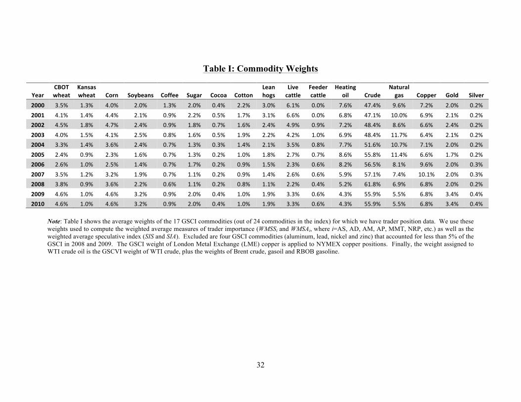
commodity futures contracts. Because it uses weights that reflect each commodity’s worldwide

production figures, it is heavily tilted toward energy (see Table I). In robustness checks, we

therefore use another widely used unlevered investable benchmark, the Dow-Jones-UBS

Commodity Index Total Return (DJ-UBSCITR; DJ-AIGTR till May 2009). This rolling index

covers 19 physical commodities in our sample period and offers a more “diversified benchmark

for the commodity futures market.” We find similar results for the GSCI and DJ-UBS indices,

and therefore we mainly discuss the GSCI.

For equities, we use Standard and Poor’s S&P 500 index. This stock index is broad-

based, making it a natural choice. Furthermore, the trading activity in the Chicago Mercantile

Exchange’s S&P 500 e-Mini futures far exceeds that of other equity-index futures in the United

States, making the S&P 500 e-Mini the ideal market in which to test the hypothesis that cross-

market traders may contribute to commodity-equity linkages. We find similar DCC patterns

using Dow-Jones' Industrial Average (DJIA) index, and therefore we focus our discussion on the

S&P500.5 For comparison purposes, we also provide figures for the (generally slightly higher)

correlations between the GSCI and the MSCI World Equity index (MSCI).

4 Precisely, we measure the percentage rate of return on the Ith investable index in period t as rI

t = 100 Log(PIt / PI

t-1), where PI

t is the value of index I at time t. 5 Our equity index returns omit dividends and, hence, underestimate actual returns (Shoven and Sialm, 2000). However, insofar as large U.S. corporations either smooth dividend payments over time (Allen and Michaely, 2002) or do not pay dividends, the correlation estimates that are the focus of our paper should be essentially unaffected.

8

B. Descriptive statistics

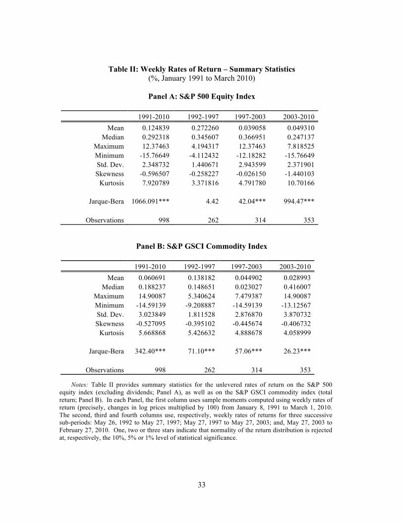
Table II presents descriptive statistics for the weekly rates of return on the S&P 500

equity index (Panel A) and on the S&P GSCI commodity index (Panel B).

From January 1991 through February 2010, the mean weekly total rate of return on the

GSCI was 0.0606% (or 3.16% in annualized terms), with a minimum of -14.59% and a

maximum of 14.90%. The typical rate of return varied sharply across the sample period: it

averaged 0.14% in 1992-1997 (7.45 % annualized); 0.045% in 1997-2003 (or a mere 2.36%

annualized); and 0.0290% in 2003-2010 (1.51% annualized).

From January 1991 through February 2010, the mean weekly rate of return on the S&P

500 was on average higher than the return on a commodity investment: 0.125% (or 6.71% in

annualized terms), with a minimum of –15.77% and a maximum of 12.37%. However, as also

noted by Büyük!ahin, Haigh and Robe (2010), the rank-ordering of the returns on the two asset

classes fluctuates dramatically over time: whereas equities massively outperformed commodities

in 1992-1997, the reverse happened in 2003-2008. At the very least, these differences show that

equities and commodities do not move in lockstep.

Turning to volatility, Table II shows that the rate of return on a well-diversified basket of

equities (S&P 500) is generally less volatile than that on commodities (GSCI). The standard

deviation of the rate of return on commodities was particularly high after 2003.

C. Dynamic Conditional Correlations

Our main interest is in the relationship between commodity and equity returns at various

points in time. With unconditional techniques such as rolling correlations or exponential

smoothing, the sensitivity of the estimated correlations to volatility changes restricts inferences

about the true nature of the relationship between variables, and periods of high volatility only

magnify concerns of heteroskedasticity biases – see Forbes and Rigobon (2002). Consequently,

we use the dynamic conditional correlation (DCC) methodology of Engle (2002) in order to

obtain dynamically correct estimates of the intensity of commodity-equity co-movements.

In essence, the DCC model is based on a two-step approach to estimating the time-

varying correlation between two series. First, we estimate time-varying variances using a

GARCH(p,q) model. For our sample, p=q=1. Second, we estimate a time-varying correlation

matrix using the standardized residuals from the first-stage estimation.

9

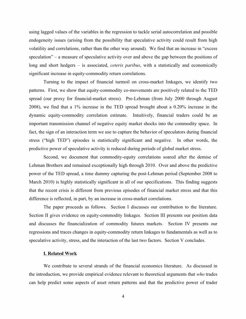
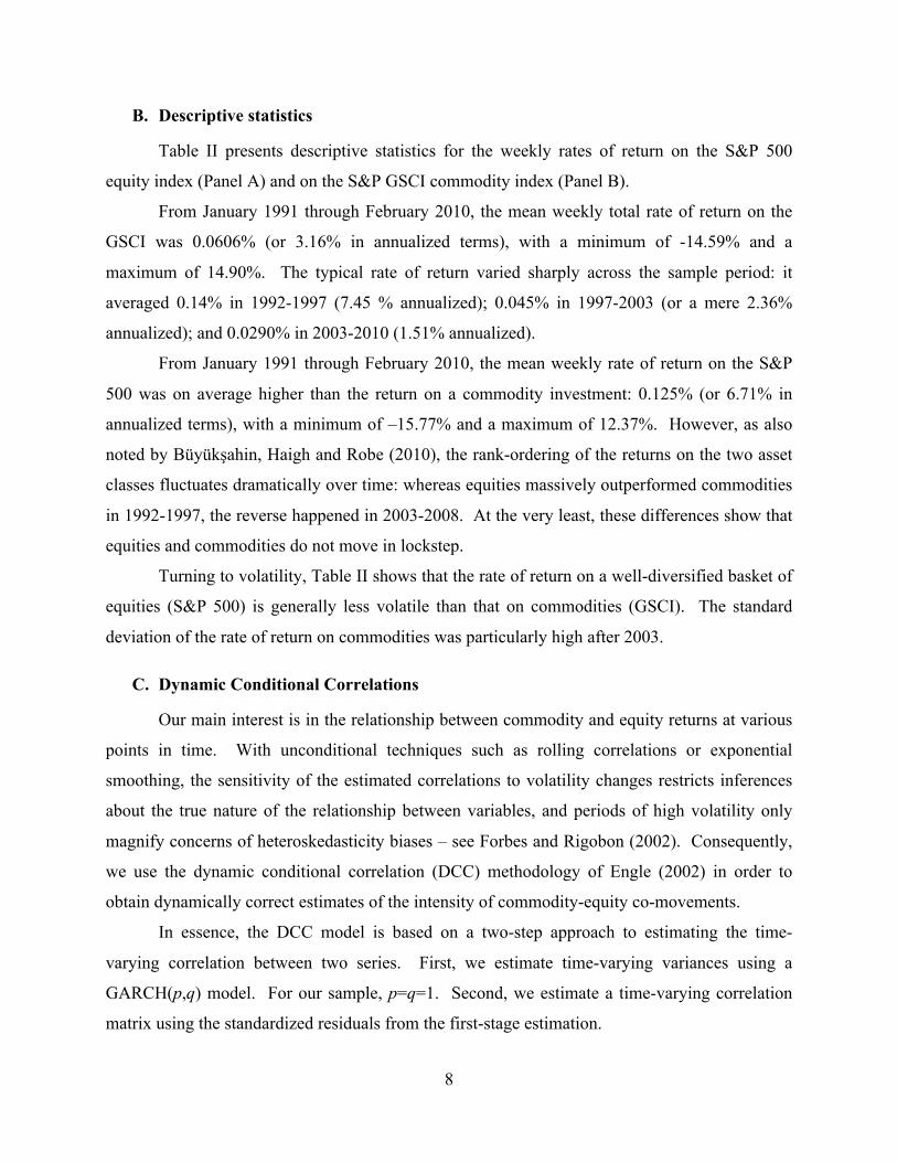
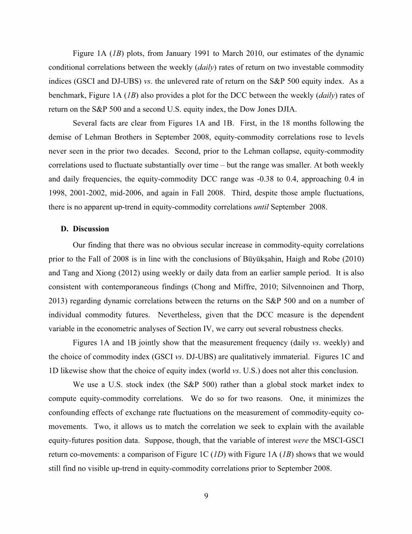
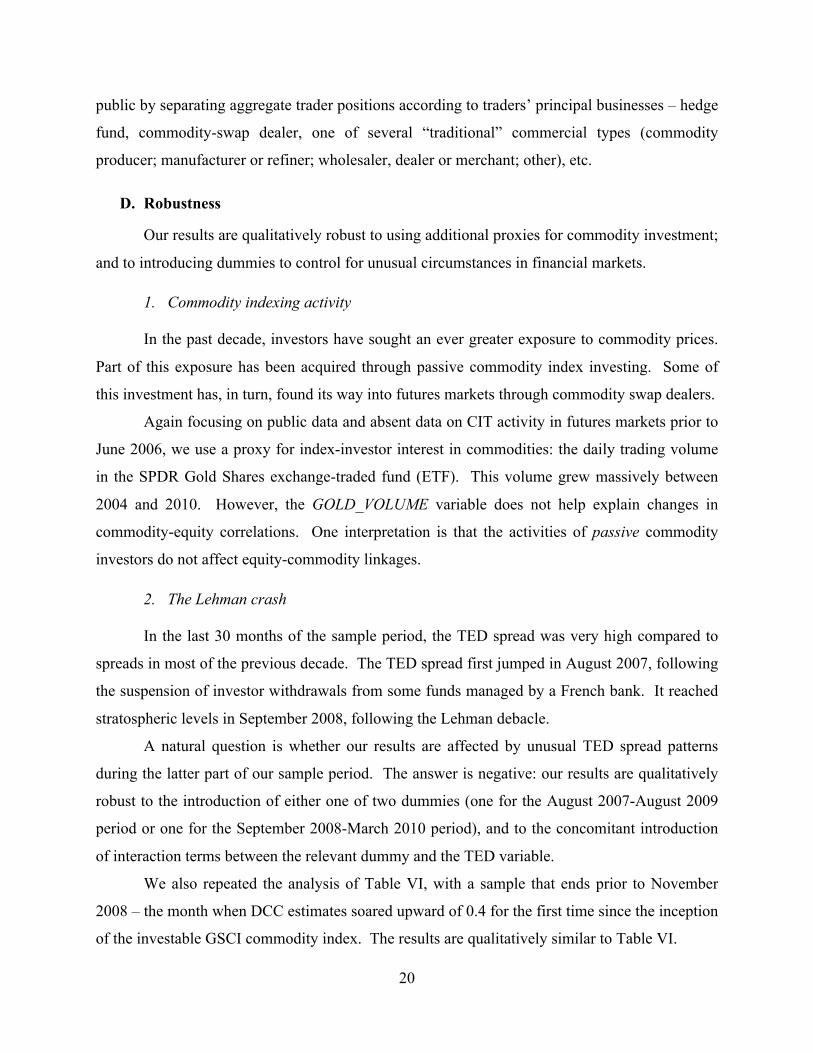
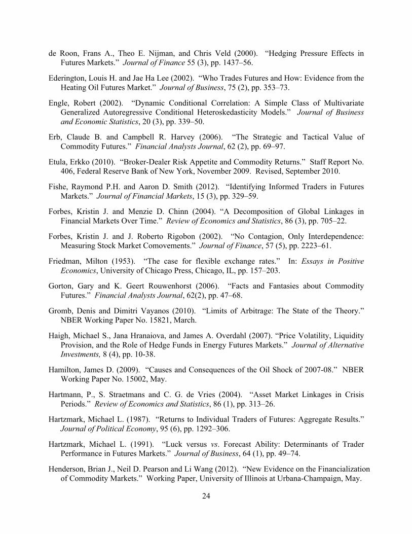
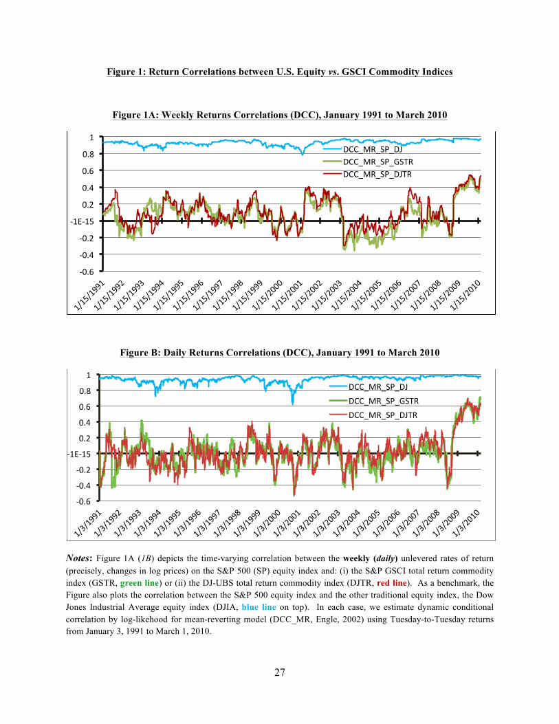
Figure 1A (1B) plots, from January 1991 to March 2010, our estimates of the dynamic

conditional correlations between the weekly (daily) rates of return on two investable commodity

indices (GSCI and DJ-UBS) vs. the unlevered rate of return on the S&P 500 equity index. As a

benchmark, Figure 1A (1B) also provides a plot for the DCC between the weekly (daily) rates of

return on the S&P 500 and a second U.S. equity index, the Dow Jones DJIA.

Several facts are clear from Figures 1A and 1B. First, in the 18 months following the

demise of Lehman Brothers in September 2008, equity-commodity correlations rose to levels

never seen in the prior two decades. Second, prior to the Lehman collapse, equity-commodity

correlations used to fluctuate substantially over time – but the range was smaller. At both weekly

and daily frequencies, the equity-commodity DCC range was -0.38 to 0.4, approaching 0.4 in

1998, 2001-2002, mid-2006, and again in Fall 2008. Third, despite those ample fluctuations,

there is no apparent up-trend in equity-commodity correlations until September 2008.

D. Discussion

Our finding that there was no obvious secular increase in commodity-equity correlations

prior to the Fall of 2008 is in line with the conclusions of Büyük!ahin, Haigh and Robe (2010)

and Tang and Xiong (2012) using weekly or daily data from an earlier sample period. It is also

consistent with contemporaneous findings (Chong and Miffre, 2010; Silvennoinen and Thorp,

2013) regarding dynamic correlations between the returns on the S&P 500 and on a number of

individual commodity futures. Nevertheless, given that the DCC measure is the dependent

variable in the econometric analyses of Section IV, we carry out several robustness checks.

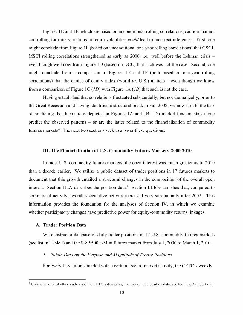
Figures 1A and 1B jointly show that the measurement frequency (daily vs. weekly) and

the choice of commodity index (GSCI vs. DJ-UBS) are qualitatively immaterial. Figures 1C and

1D likewise show that the choice of equity index (world vs. U.S.) does not alter this conclusion.

We use a U.S. stock index (the S&P 500) rather than a global stock market index to

compute equity-commodity correlations. We do so for two reasons. One, it minimizes the

confounding effects of exchange rate fluctuations on the measurement of commodity-equity co-

movements. Two, it allows us to match the correlation we seek to explain with the available

equity-futures position data. Suppose, though, that the variable of interest were the MSCI-GSCI

return co-movements: a comparison of Figure 1C (1D) with Figure 1A (1B) shows that we would

still find no visible up-trend in equity-commodity correlations prior to September 2008.

10

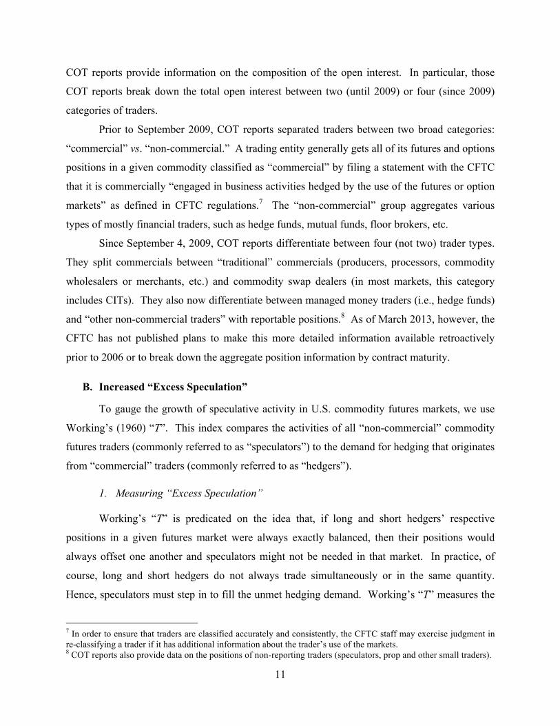
Figures 1E and 1F, which are based on unconditional rolling correlations, caution that not

controlling for time-variations in return volatilities could lead to incorrect inferences. First, one

might conclude from Figure 1F (based on unconditional one-year rolling correlations) that GSCI-

MSCI rolling correlations strengthened as early as 2006, i.e., well before the Lehman crisis –

even though we know from Figure 1D (based on DCC) that such was not the case. Second, one

might conclude from a comparison of Figures 1E and 1F (both based on one-year rolling

correlations) that the choice of equity index (world vs. U.S.) matters – even though we know

from a comparison of Figure 1C (1D) with Figure 1A (1B) that such is not the case.

Having established that correlations fluctuated substantially, but not dramatically, prior to

the Great Recession and having identified a structural break in Fall 2008, we now turn to the task

of predicting the fluctuations depicted in Figures 1A and 1B. Do market fundamentals alone

predict the observed patterns – or are the latter related to the financialization of commodity

futures markets? The next two sections seek to answer these questions.

III. The Financialization of U.S. Commodity Futures Markets, 2000-2010

In most U.S. commodity futures markets, the open interest was much greater as of 2010

than a decade earlier. We utilize a public dataset of trader positions in 17 futures markets to

document that this growth entailed a structural changes in the composition of the overall open

interest. Section III.A describes the position data.6 Section III.B establishes that, compared to

commercial activity, overall speculative activity increased very substantially after 2002. This

information provides the foundation for the analyses of Section IV, in which we examine

whether participatory changes have predictive power for equity-commodity returns linkages.

A. Trader Position Data

We construct a database of daily trader positions in 17 U.S. commodity futures markets

(see list in Table I) and the S&P 500 e-Mini futures market from July 1, 2000 to March 1, 2010. 1. Public Data on the Purpose and Magnitude of Trader Positions

For every U.S. futures market with a certain level of market activity, the CFTC’s weekly

6 Only a handful of other studies use the CFTC’s disaggregated, non-public position data: see footnote 3 in Section I.

11

COT reports provide information on the composition of the open interest. In particular, those

COT reports break down the total open interest between two (until 2009) or four (since 2009)

categories of traders.

Prior to September 2009, COT reports separated traders between two broad categories:

“commercial” vs. “non-commercial.” A trading entity generally gets all of its futures and options

positions in a given commodity classified as “commercial” by filing a statement with the CFTC

that it is commercially “engaged in business activities hedged by the use of the futures or option

markets” as defined in CFTC regulations.7 The “non-commercial” group aggregates various

types of mostly financial traders, such as hedge funds, mutual funds, floor brokers, etc.

Since September 4, 2009, COT reports differentiate between four (not two) trader types.

They split commercials between “traditional” commercials (producers, processors, commodity

wholesalers or merchants, etc.) and commodity swap dealers (in most markets, this category

includes CITs). They also now differentiate between managed money traders (i.e., hedge funds)

and “other non-commercial traders” with reportable positions.8 As of March 2013, however, the

CFTC has not published plans to make this more detailed information available retroactively

prior to 2006 or to break down the aggregate position information by contract maturity.

B. Increased “Excess Speculation”

To gauge the growth of speculative activity in U.S. commodity futures markets, we use

Working’s (1960) “T”. This index compares the activities of all “non-commercial” commodity

futures traders (commonly referred to as “speculators”) to the demand for hedging that originates

from “commercial” traders (commonly referred to as “hedgers”). 1. Measuring “Excess Speculation”

Working’s “T” is predicated on the idea that, if long and short hedgers’ respective

positions in a given futures market were always exactly balanced, then their positions would

always offset one another and speculators might not be needed in that market. In practice, of

course, long and short hedgers do not always trade simultaneously or in the same quantity.

Hence, speculators must step in to fill the unmet hedging demand. Working’s “T” measures the

7 In order to ensure that traders are classified accurately and consistently, the CFTC staff may exercise judgment in re-classifying a trader if it has additional information about the trader’s use of the markets. 8 COT reports also provide data on the positions of non-reporting traders (speculators, prop and other small traders).

12

extent to which speculation is in “excess” of the level required to offset any unbalanced hedging

at the market-clearing price (i.e., to satisfy hedgers’ net demand for hedging at that price).

Despite its possibly confusing name, it is worth noting that “excess” speculation thus defined

may not be “excessive” in that some “excess” speculation may be economically necessary in the

presence of friction such as the mismatch in timing and maturity of trading contracts.

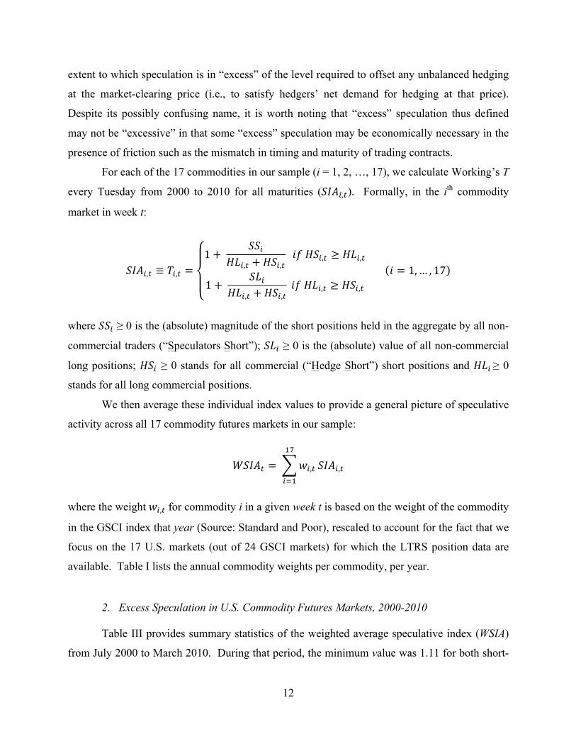
For each of the 17 commodities in our sample (i = 1, 2, …, 17), we calculate Working’s T

every Tuesday from 2000 to 2010 for all maturities (!"#!!!). Formally, in the ith commodity

market in week t:

!"#!!! ! !!!! !!! ! !!!

!"!!! ! !"!!!!!!"!!"!!! ! !"!!!

!! ! !"!!"!!! ! !"!!!

!!"!!"!!! ! !"!!!!!!!!!! ! ! !!! ! !"

where !!! " 0 is the (absolute) magnitude of the short positions held in the aggregate by all non-

commercial traders (“Speculators Short”); !"! " 0 is the (absolute) value of all non-commercial

long positions; !"! " 0 stands for all commercial (“Hedge Short”) short positions and !"!!" 0

stands for all long commercial positions.

We then average these individual index values to provide a general picture of speculative

activity across all 17 commodity futures markets in our sample:

!"#$! ! ! !!!!!"

!!!!"#!!!

where the weight !!!!!for commodity i in a given week t is based on the weight of the commodity

in the GSCI index that year (Source: Standard and Poor), rescaled to account for the fact that we

focus on the 17 U.S. markets (out of 24 GSCI markets) for which the LTRS position data are

available. Table I lists the annual commodity weights per commodity, per year.

2. Excess Speculation in U.S. Commodity Futures Markets, 2000-2010

Table III provides summary statistics of the weighted average speculative index (WSIA)

from July 2000 to March 2010. During that period, the minimum value was 1.11 for both short-

13

term and all contracts; the maximum was 1.42 across all maturities. In other words, speculative

positions were on average 11% to 42% greater than what was minimally necessary to meet net

hedging needs at the market-clearing prices.

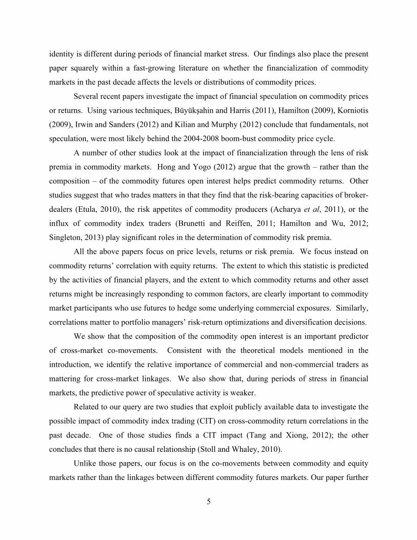
Figure 2 documents the growing importance of speculation in commodity markets in the

past decade. Excess speculation increased substantially, from about 11% in 2000 to about 40-

50% in 2008.9 Notably, excess speculation fell after 2008. An interesting question, the answer to

which would require more disaggregated data than are publicly available, is whether excess

speculation in near-dated contracts is greater than it is further out on the maturity curve.

In sum, Figure 2 identifies a long-term increase, but also substantial variations, in excess

commodity speculation. Those patterns will be of particular interest in the analysis of Section IV.

IV. Economic Fundamentals, Speculation and Commodity-Equity Co-movements

In Section II, we showed that the conditional correlation between the weekly returns on

investible equity and commodity indices fluctuates substantially over time. In Section III, we

provided a speculative activity index to summarize various aspects of financialization in U.S.

commodity futures markets in the last decade.

Figure 2 suggests that the patterns exhibited by the index of “excess” speculation bear at

least some resemblance with the equity-commodity returns correlation patterns. In this Section,

we ask formally whether long-term fluctuations in the intensity of speculative activity can help

predict the extent to which commodity returns move in sync with equity returns. Besides

speculative activity, of course, prior literature suggests that economic fundamentals and financial

market stress should influence commodity-equity return correlations. Section IV.A therefore

introduces our real-sector and financial-sector controls. Section IV.B discusses our ARDL

regression methodology, which tackles possible endogeneity issues as well as the fact that some

of our variables are stationary in levels while others are only stationary in first differences.

Section IV.C presents our regression results.

Tables III.A-B provide summary statistics for all the variables. Table IV provides simple

cross-correlations between the macro variables. Tables V-VIII summarize our regression results.

9 The values in Figure 2 are generally lower than historical T values for agricultural commodities. Peck (1981) gets values of 1.57-2.17; Leuthold (1983), values of 1.05-2.34. See also Irwin, Merrin and Sanders (2008).

14

A. Real Sector and Financial-Market Conditions

1. Macroeconomic Fundamentals

Business cycle factors affect commodity returns (e.g., Erb and Harvey, 2006; Gorton and

Rouwenhorst, 2006). Furthermore, the response of U.S. stock returns to crude oil price increases

depends on whether the increases are the result of a demand shock or of a supply shock in the

crude oil space (Kilian and Park, 2009). These empirical facts point to the need to control for

real-sector factors when explaining time variations in the strength of equity-commodity linkages.

To do so, we use a measure of global real economic activity proposed by Kilian (2009),

who shows that “increases in freight (shipping) rates may be used as indicators of (…) demand

shifts in global industrial commodity markets.” The Kilian measure is a global index of single-

voyage freight rates for bulk dry cargoes including grain, oilseeds, coal, iron ore, fertilizer and

scrap metal. This index accounts for the existence of “different fixed effects for different routes,

commodities and ship sizes.” It is deflated with the U.S. consumer price index (CPI) and

linearly detrended to remove the impact of the “secular decrease in the cost of shipping dry cargo

over the last forty years.” This indicator is available monthly from 1968. We derive weekly

estimates (which we denote SHIP) by cubic spline.

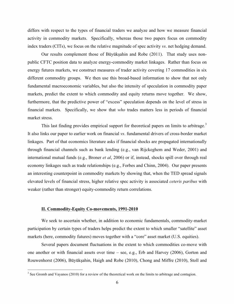
Table III contains summary statistics for SHIP. Figure 3, which charts its value from

2000 to 2010, shows an inverse long-term relationship between SHIP and our DCC estimates –

suggesting that correlations increase when world demand for commodities is low.

While SHIP provides a measure of worldwide economic activity, U.S. macroeconomic

conditions are central to U.S. equity prices and could affect commodity prices. Consequently,

we also consider two macroeconomic variables that may be relevant when studying commodity-

equity relationships. One, denoted ADS, is the Aruoba-Diebold-Scotti (2009) gauge of U.S.

economic activity. It is available weekly for the entire sample period (1991-2010). The other

variable captures U.S. inflationary expectations and the intuition that commodities may provide a

better hedge against inflation than equities do. We use the figures released each month by the

Federal Reserve Bank of Cleveland and carry out a linear interpolation to derive weekly figures,

denoted INF. Table III provides summary statistics for these two macroeconomic indicators.

15

2. Financial Stress and Lehman Crisis

Cross-market co-movements increase amid financial stress. Hartmann, Straetmans and

de Vries (2004) identify cross-asset extreme linkages in the case of bond and equity returns from

the G-5 countries. Similarly, Longin and Solnik (2001) find that international equity market

correlations increase in bear markets. For commodities, Büyük!ahin, Haigh and Robe (2010)

show that commodity and equity markets behave like a “market of one” during extreme events.

We account for this reality in two ways.

First, we include the TED spread in our regressions as a proxy of financial market stress.

Table III provides statistical information on the TED variable. The TED spread varied widely

during our sample period, with a minimum of 0.027% and a maximum of 4.33%.

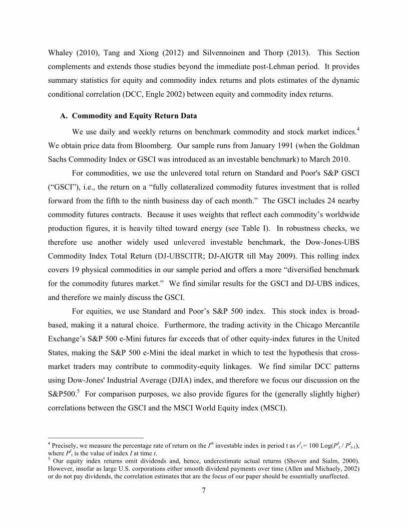
Second, Figure 4 shows that the TED spread, though particularly high after the onset of

the Lehman crisis, had already started rising in the previous 13 months (starting in August 2007

when a French financial group froze two funds exposed to the sub-prime market). In contrast,

equity-commodity correlations did not visibly increase until after the demise of Lehman Brothers

in September 2008. They remained exceptionally high through the end of our sample in 2010.

This difference suggests that the post-Lehman period is exceptional. We use a time dummy

(DUM) to account for specificities of this sub-period that the TED spread might not capture.

B. Methodology

Before testing the predictive power of different variables on the DCC between equity and

commodity returns, we check the order of integration of each variable using Augmented Dickey

Fuller (ADF) tests. Unit root tests for the variables in our estimation equation are summarized at

the bottoms of Tables III.A and III.B. They show that some of the variables are I(1) whereas the

rest are I(0).

By construction, correlations are bounded above (+1) and below (-1) so the DCC variable

should intuitively be stationary. Yet, the ADF tests do not reject the non-stationarity of the DCC

estimates in our sample period. This result holds at the 1% level of significance for the entire

sample period (2000-2010, see Table III) and at the 10% level of significance for a sub-sample

ending prior to the demise of Lehman Brothers (2000 to September 2008).10

10 Because it is well known that ADF tests have low power with short time spans of data, we also employ another test developed by Kwiatkowski et al (KPSS, 1992) to further analyze the DCC variable. Unlike the ADF test, the

16

In order to find the long run effects of different variables on commodity-equity return

correlations, we use an autoregressive distributed lag (ARDL) model estimated by ordinary least

squares. In this model, the dynamic conditional correlation is explained by lags of itself and

current and lagged values of a number of regressors (fundamentals as well as traders’ positions).

The lagged values of the dependent variable are included to account for slow adjustment of the

correlation between commodities and equities. This approach also allows us to calculate the

long-run effect of the regressors on the correlation. If our DCC measure is, in fact, stationary,

then the ARDL model, estimated by OLS, should give us consistent parameter estimates. If our

DCC variable is non-stationary, as suggested by the ADF test statistics, then both short-run and

long-run parameters in the ARDL model can still be consistently estimated by OLS if there is a

single cointegrating relationship (Pesaran and Shin, 1999).

Specifically, Pesaran and Shin (1999) show that the ARDL model can be used to test the

existence of a long-run relationship between underlying variables and to provide consistent,

unbiased estimators of long-run parameters in the presence of I(0) and I(1) regressors. The

ARDL estimation procedure reduces the bias in the long run parameter in finite samples and

ensures that it has a normal distribution irrespective of whether the underlying regressors are I(0)

or I(1). By choosing appropriate orders of the ARDL(p,q) model, Pesaran and Shin (1999) show

that the ARDL model simultaneously corrects for residual correlation and for the problem of

endogenous regressors.

We start with the problem of estimation and hypothesis testing in the context of the

following ARDL(p,q) model:

!!!!!!!!!!!!!!!!!!!!!!!!!!!!!!!!!!!!!!!!!!!!!!!!!!!!!!!!!!! ! !"! ! !!!!!!!

!!!! !!!!!!

!

!!!! !!!!!!!!!!!!!!!!!!!!!!!!!!!!!!!!!!!!!!!!

where y is a t ! 1 vector of the dependent variable, x is a t ! k vector of regressors, and ! stands

for a t x s vector of deterministic variables such as an intercept, seasonal dummies, time trends,

or exogenous variables with fixed lags.11 In vector notation, Equation (1) is:

KPSS test has stationarity as the null hypothesis. With the KPSS test, we find that the null of stationarity cannot be rejected at the 5% level of significance but is rejected at the 10% significance level. 11 The error term is assumed to be serially uncorrelated.

17

!!!!!! ! !"! ! !!!!!!! ! !!

where !!!! is the polynomial lag operator !! !!! ! !!!! !! !!!!; !!!! is the polynomial lag

operator !! ! !!! ! !!!! !!! !!!!; and L represents the usual lag operator (!!!! ! !!!!).

The estimate of the long run parameters can then be obtained by first estimating the parameters

of the ARDL model by OLS and then solving the estimated version of (1) for the cointegrating

relationship !! ! !"! ! !!"! ! !!! by:

! ! !! ! !! !!! !!!! !! ! !! !!! !!

! ! !!! !! ! !! !!! !!

where ! gives us the long-run response of y to a unit change in x and, similarly, ! represents the

long run response of y to a unit change in the deterministic exogenous variable.

When estimating the long-run relationship, one of the most important issues is the choice

of the order of the distributed lag function on !! and the explanatory variables !!. We carry out

a two-step ARDL estimation approach proposed by Pesaran and Shin (1999). First, the lag

orders of p and q must be selected using some information criterion. Based on Monte Carlo

experiments, Pesaran and Shin (1999) argue that the Schwarz criterion performs better than other

criteria. This criterion suggests optimal lag lengths p=1 and q=1 in our case. Second, we

estimate the long run coefficients and their standard errors using the ARDL(1,1) specification.

C. Regression Results

Tables V to VIII sumarize our regression results. Table V establishes the predictive

power of economic fundamentals (SHIP and, to a lesser extent, ADS) and financial stress (TED).

Table VI establishes the additional predictive power of speculative activities.

1. Real sector and financial stress variables

Panels A and B in Table V show that, for our sample period (2000-2010) as well as for an

extended period (1991-2000, starting when the GSCI first became investable but before the start

of our detailed position dataset), the commodity-equity DCC measure is statistically significantly

18

negatively related to SHIP. Insofar as SHIP captures world demand for commodities, this finding

confirms the intuition that cross-market correlations increase in globally bad economic times.

Our two U.S. macroeconomic indicators (ADS and INF) have less explanatory power.

The coefficient for ADS is consistently positive but is not always statistically significant.

Intuitively, if equities and commodities respond differently to high inflation, then DCC and INF

should be negatively related. Column 7 of Panel A (using data from 1991-2010) supports this

prediction. In most of our other regressions, however, INF is not statistically significant. As

Gorton and Rouwenhorst (2006) note, asset returns are volatile relative to inflation; consequently,

longer-term correlations better capture the inflation properties of commodity and equity investments.

The lack of significance of INF, especially in regressions using data from 2000-2010 only, may

therefore be a mere artifact of sample length.

All of our models include a variable capturing momentum in equity markets (denoted

UMD). This variable always has a positive coefficient (consistent with the notion that equity

momentum could spill over into other risky assets such as commodities), but we never find UMD

to be a statistically significant predictor of commodity-equity correlations.

The difference between Panels A and B in Table V is that the specifications in Panel B

include a dummy for the post-Lehman period (DUM). That time dummy is always strongly

statistically significant and positive, supporting graphical evidence (see Section II) that this sub-

period is exceptional.

Our ARDL estimates show that commodity-equity return correlations also have a positive

long-term relationship to our proxy for stress in financial markets (TED). In 2000-2010, a 1%

increase in the TED spread brought about a 0.20 to 0.30% increase in the dynamic equity-

commodity correlation; this increase is statistically significant at the 5% level of confidence (at

the 1% level in 2000-2008; table available upon request).

Interestingly, Panel A suggests that TED was not a significant factor in 1991-2000. The

difference in the TED spread’s importance in those two successive decades suggests a possible

role for trading activity. We next turn to this issue. 2. Speculative activity

Table VI shows that trading activity in commodity futures markets helps predict long-

term changes in commodity-equity linkages. Specifically, after controlling for economic

19

fundamentals, “excess” speculation in commodity futures markets helps predict the fluctuations

in the commodity-equity DCC estimates over time. Ceteris paribus, an increase of 1% in the

speculative index (WSIA) is associated with dynamic conditional equity-commodity correlations

that are approximately 4% to 7% higher (given a mean excess spec index of about 25%).

Intuitively, Working’s “T” index of excess speculation in commodity futures markets,

which aggregates the activities of all non-hedgers across all maturities, should have less

predictive power than a measure of hedge fund activity in short-dated contracts. Similarly, the

activities hedge funds that trade in both equity and commodity markets might better predict long-

term linkages between equity and commodity returns. If so, this would suggest that it is value

arbitrageurs’ willingness to take positions in both equity and commodity markets, rather than the

trading activities of more traditional commodity market participants, that help link satellite and

central markets. Answering these questions, however, requires disaggregated data and is left for

another draft. 3. Interaction between speculation and financial stress

Table VI shows that greater “excess” speculation is associated with enhanced cross-

market linkages. Yet if the same arbitrageurs or convergence traders, who bring markets

together during normal times, face borrowing constraints or other pressures to liquidate risky

positions during periods of financial market stress, then their exit from “satellite markets” after a

major shock in a “central” market could lead to a decoupling of the markets that they had helped

link in the first place.

Building on this hypothesis, some specifications in Table VI include an interaction term

that captures the behavior of speculators during financial stress episodes. This interaction term is

almost always statistically significant and is always (as expected) negative. That is, ceteris

paribus, speculative activity is less helpful in predicting commodity-equity return co-movements

during periods of elevated market stress. 4. Implications for portfolio management

Our results suggest that non-public information on the composition of commodity futures

open interest (or, more generally, the make-up of trading activity in financial markets) could be

relevant to asset allocation decisions. A corollary is that portfolio managers could benefit from a

recent CFTC decision to disaggregate the position information that it makes available to the

20

public by separating aggregate trader positions according to traders’ principal businesses – hedge

fund, commodity-swap dealer, one of several “traditional” commercial types (commodity

producer; manufacturer or refiner; wholesaler, dealer or merchant; other), etc.

D. Robustness

Our results are qualitatively robust to using additional proxies for commodity investment;

and to introducing dummies to control for unusual circumstances in financial markets. 1. Commodity indexing activity

In the past decade, investors have sought an ever greater exposure to commodity prices.

Part of this exposure has been acquired through passive commodity index investing. Some of

this investment has, in turn, found its way into futures markets through commodity swap dealers.

Again focusing on public data and absent data on CIT activity in futures markets prior to

June 2006, we use a proxy for index-investor interest in commodities: the daily trading volume

in the SPDR Gold Shares exchange-traded fund (ETF). This volume grew massively between

2004 and 2010. However, the GOLD_VOLUME variable does not help explain changes in

commodity-equity correlations. One interpretation is that the activities of passive commodity

investors do not affect equity-commodity linkages. 2. The Lehman crash

In the last 30 months of the sample period, the TED spread was very high compared to

spreads in most of the previous decade. The TED spread first jumped in August 2007, following

the suspension of investor withdrawals from some funds managed by a French bank. It reached

stratospheric levels in September 2008, following the Lehman debacle.

A natural question is whether our results are affected by unusual TED spread patterns

during the latter part of our sample period. The answer is negative: our results are qualitatively

robust to the introduction of either one of two dummies (one for the August 2007-August 2009

period or one for the September 2008-March 2010 period), and to the concomitant introduction

of interaction terms between the relevant dummy and the TED variable.

We also repeated the analysis of Table VI, with a sample that ends prior to November

2008 – the month when DCC estimates soared upward of 0.4 for the first time since the inception

of the investable GSCI commodity index. The results are qualitatively similar to Table VI.

21

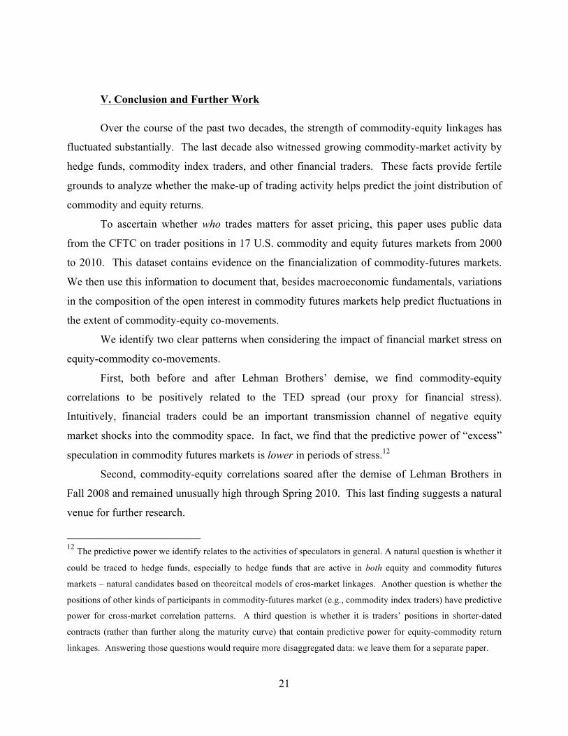
V. Conclusion and Further Work

Over the course of the past two decades, the strength of commodity-equity linkages has

fluctuated substantially. The last decade also witnessed growing commodity-market activity by

hedge funds, commodity index traders, and other financial traders. These facts provide fertile

grounds to analyze whether the make-up of trading activity helps predict the joint distribution of

commodity and equity returns.

To ascertain whether who trades matters for asset pricing, this paper uses public data

from the CFTC on trader positions in 17 U.S. commodity and equity futures markets from 2000

to 2010. This dataset contains evidence on the financialization of commodity-futures markets.

We then use this information to document that, besides macroeconomic fundamentals, variations

in the composition of the open interest in commodity futures markets help predict fluctuations in

the extent of commodity-equity co-movements.

We identify two clear patterns when considering the impact of financial market stress on

equity-commodity co-movements.

First, both before and after Lehman Brothers’ demise, we find commodity-equity

correlations to be positively related to the TED spread (our proxy for financial stress).

Intuitively, financial traders could be an important transmission channel of negative equity

market shocks into the commodity space. In fact, we find that the predictive power of “excess”

speculation in commodity futures markets is lower in periods of stress.12

Second, commodity-equity correlations soared after the demise of Lehman Brothers in

Fall 2008 and remained unusually high through Spring 2010. This last finding suggests a natural

venue for further research.

12 The predictive power we identify relates to the activities of speculators in general. A natural question is whether it

could be traced to hedge funds, especially to hedge funds that are active in both equity and commodity futures

markets – natural candidates based on theoreitcal models of cros-market linkages. Another question is whether the

positions of other kinds of participants in commodity-futures market (e.g., commodity index traders) have predictive

power for cross-market correlation patterns. A third question is whether it is traders’ positions in shorter-dated

contracts (rather than further along the maturity curve) that contain predictive power for equity-commodity return

linkages. Answering those questions would require more disaggregated data: we leave them for a separate paper.

22

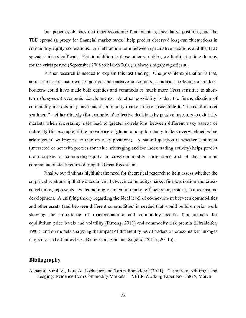
Our paper establishes that macroeconomic fundamentals, speculative positions, and the

TED spread (a proxy for financial market stress) help predict observed long-run fluctuations in

commodity-equity correlations. An interaction term between speculative positions and the TED

spread is also significant. Yet, in addition to those other variables, we find that a time dummy

for the crisis period (September 2008 to March 2010) is always highly significant.

Further research is needed to explain this last finding. One possible explanation is that,

amid a crisis of historical proportion and massive uncertainty, a radical shortening of traders’

horizons could have made both equities and commodities much more (less) sensitive to short-

term (long-term) economic developments. Another possibility is that the financialization of

commodity markets may have made commodity markets more susceptible to “financial market

sentiment” – either directly (for example, if collective decisions by passive investors to exit risky

markets when uncertainty rises lead to greater correlations between different risky assets) or

indirectly (for example, if the prevalence of gloom among too many traders overwhelmed value

arbitrageurs’ willingness to take on risky positions). A natural question is whether sentiment

(interacted or not with proxies for value arbitraging and for index trading activity) helps predict

the increases of commodity-equity or cross-commodity correlations and of the common

component of stock returns during the Great Recession.

Finally, our findings highlight the need for theoretical research to help assess whether the

empirical relationship that we document, between commodity-market financialization and cross-

correlations, represents a welcome improvement in market efficiency or, instead, is a worrisome

development. A unifying theory regarding the ideal level of co-movement between commodities

and other assets (and between different commodities) is needed that would build on prior work

showing the importance of macroeconomic and commodity-specific fundamentals for

equilibrium price levels and volatility (Pirrong, 2011) and commodity risk premia (Hirshleifer,

1988), and on models analyzing the impact of different types of traders on cross-market linkages

in good or in bad times (e.g., Danielsson, Shin and Zigrand, 2011a, 2011b).

Bibliography

Acharya, Viral V., Lars A. Lochstoer and Tarun Ramadorai (2011). “Limits to Arbitrage and Hedging: Evidence from Commodity Markets.” NBER Working Paper No. 16875, March.

23

Allen, Franklin and Roni Michaely (2002). “Payout Policy.” In Constantinides, G., Harris, M., and Stulz, R. [Eds.], Handbook of Financial Economics. North-Holland.

Aruoba, S. Bora#an, Francis X. Diebold, Chiara Scotti (2009). “Real-time Measurement of

Business Conditions.” Journal of Business and Economic Statistics. 27 (4), pp. 417–27. Ba!ak, Süleyman and Benjamin Croitoru (2006). “On the Role of Arbitrageurs in Rational

Markets.” Journal of Financial Economics, 81 (1), pp. 143–73. Bessembinder, Hendrik (1992). “Systematic Risk, Hedging Pressure, and Risk Premiums in

Futures Markets.” Review of Financial Studies, 5 (4), pp. 637–67. Broner, Fernando A., R. Gaston Gelos and Carmen M. Reinhart (2008). “When in Peril,

Retrench: Testing the Portfolio Channel of Contagion.” Journal of International Economics, 69 (1), pp. 203–30.

Brunetti, Celso, Bahattin Büyük!ahin and Harris, Jeffrey H. (2011). “Speculators, Prices and

Market Volatility.” Working Paper, International Energy Agency, January. Brunetti, Celso and David Reiffen (2011). “Commodity Index Trading and Hedging Costs.”

Federal Reserve Board Finance & Economics Discussion Series Paper 2011–57, August. Büyük!ahin, Bahattin, Michael S. Haigh, Jeffrey H. Harris, James A. Overdahl, J.A., and Michel

A. Robe (2009). “Fundamentals, Trading Activity and Derivative Pricing.” Paper presented at the 2009 Meeting of the European Finance Association.

Büyük!ahin, Bahattin, Michael S. Haigh and Michel A. Robe (2010). “Commodities and

Equities: Ever a ‘Market of One’?” Journal of Alternative Investments, 12 (3), pp. 75–95. Büyük!ahin, Bahattin and Michel A. Robe (2010). “Commodity Traders' Positions and Crude

Oil Prices: Evidence from the Recent Boom-Bust Cycle.” Paper presented at the 2010 American Economic Association Meeting, Atlanta, January.

Chang, Eric C., J. Michael Pinegar and Barry Schachter (1997). “Interday Variations in Volume,

Variance and Participation of Large Speculators Source.” Journal of Banking and Finance, 21 (6), pp. 797–810.

Cheng, Ing-Haw, Andrei Kirilenko and Wei Xiong (2012). “Convective Risk Flows in

Commodity Futures Markets.” NBER Working Paper No. 17921, March. Chong, James and Jo$lle Miffre (2010). “Conditional Return Correlations between Commodity

Futures and Traditional Assets.” Journal of Alternative Investments, 12 (3), pp. 61–75. Danielsson, Jon, Hyun Song Shin and Jean–Pierre Zigrand (2011). “Balance Sheet Capacity and

Endogenous Risk”. Working Paper, London School of Economics and Princeton University, January.

Danielsson, Jon, Hyun Song Shin and Jean–Pierre Zigrand (2011b). “Endogenous and Systemic

Risk.” In Quantifying Systemic Risk, Joseph G. Haubrich and Andrew W. Lo, Eds. Chicago, IL: University of Chicago Press, Forthcoming 2012.

24

de Roon, Frans A., Theo E. Nijman, and Chris Veld (2000). “Hedging Pressure Effects in Futures Markets.” Journal of Finance 55 (3), pp. 1437–56.

Ederington, Louis H. and Jae Ha Lee (2002). “Who Trades Futures and How: Evidence from the

Heating Oil Futures Market.” Journal of Business, 75 (2), pp. 353–73. Engle, Robert (2002). “Dynamic Conditional Correlation: A Simple Class of Multivariate

Generalized Autoregressive Conditional Heteroskedasticity Models.” Journal of Business and Economic Statistics, 20 (3), pp. 339–50.

Erb, Claude B. and Campbell R. Harvey (2006). “The Strategic and Tactical Value of

Commodity Futures.” Financial Analysts Journal, 62 (2), pp. 69–97. Etula, Erkko (2010). “Broker-Dealer Risk Appetite and Commodity Returns.” Staff Report No.

406, Federal Reserve Bank of New York, November 2009. Revised, September 2010. Fishe, Raymond P.H. and Aaron D. Smith (2012). “Identifying Informed Traders in Futures

Markets.” Journal of Financial Markets, 15 (3), pp. 329–59. Forbes, Kristin J. and Menzie D. Chinn (2004). “A Decomposition of Global Linkages in

Financial Markets Over Time.” Review of Economics and Statistics, 86 (3), pp. 705–22. Forbes, Kristin J. and J. Roberto Rigobon (2002). “No Contagion, Only Interdependence:

Measuring Stock Market Comovements.” Journal of Finance, 57 (5), pp. 2223–61. Friedman, Milton (1953). “The case for flexible exchange rates.” In: Essays in Positive

Economics, University of Chicago Press, Chicago, IL, pp. 157–203. Gorton, Gary and K. Geert Rouwenhorst (2006). “Facts and Fantasies about Commodity

Futures.” Financial Analysts Journal, 62(2), pp. 47–68. Gromb, Denis and Dimitri Vayanos (2010). “Limits of Arbitrage: The State of the Theory.”

NBER Working Paper No. 15821, March. Haigh, Michael S., Jana Hranaiova, and James A. Overdahl (2007). “Price Volatility, Liquidity

Provision, and the Role of Hedge Funds in Energy Futures Markets.” Journal of Alternative Investments, 8 (4), pp. 10-38.

Hamilton, James D. (2009). “Causes and Consequences of the Oil Shock of 2007-08.” NBER

Working Paper No. 15002, May. Hartmann, P., S. Straetmans and C. G. de Vries (2004). “Asset Market Linkages in Crisis

Periods.” Review of Economics and Statistics, 86 (1), pp. 313–26. Hartzmark, Michael L. (1987). “Returns to Individual Traders of Futures: Aggregate Results.”

Journal of Political Economy, 95 (6), pp. 1292–306. Hartzmark, Michael L. (1991). “Luck versus vs. Forecast Ability: Determinants of Trader

Performance in Futures Markets.” Journal of Business, 64 (1), pp. 49–74. Henderson, Brian J., Neil D. Pearson and Li Wang (2012). “New Evidence on the Financialization

of Commodity Markets.” Working Paper, University of Illinois at Urbana-Champaign, May.

25

Hong, Harrison and Motohiro Yogo (2012). “What Does Futures Market Interest Tell Us about

the Macroeconomy and Asset Prices?” Journal of Financial Economics, 105 (3), pp. 473–90. Irwin, Scott H., Merrin, Robert P. and Dwight R. Sanders (2008). “The Adequacy of

Speculation in Agricultural Futures Markets: Too Much of a Good Thing?” Marketing and Outlook Research Reports No.2-2008, University of Illinois at Urbana-Champaign.

Irwin, Scott H., and Dwight R. Sanders (2012). “Testing the Masters Hypothesis in Commodity

Futures Markets.” Energy Economics 34 (1), pp. 256–69. Khan, Saqib, Zeigham Khokher and Timothy Simin (2008). “Expected Commodity Futures

Returns.” Working Paper, Penn State University, July. Kilian, Lutz (2009). “Not all oil price shocks are alike: Disentangling demand and supply

shocks in the crude oil market.” American Economic Review, 99 (3), pp. 1053–69. Kilian, Lutz and Dan Murphy (2012). “The Role of Inventories and Speculative Trading in the

Global Market for Crude Oil.” CEPR Discussion Paper No. 7753, May 2010. Updated, July 2012.

Kodres, Laura E. and Matthew Pritsker (2002). “A Rational Expectations Model of Financial

Contagion.” Journal of Finance, 57 (2), pp. 1540–62. Kofman, Paul, David Michayluk, and James T. Moser (2009). “Reversing the Lead, or a Series

of Unfortunate Events? NYMEX, ICE and Amaranth.” Journal of Futures Markets, 29 (12), pp. 1130–60.

Korniotis, George M. (2009). “Does Speculation Affect Spot Price Levels? The Case of Metals

with and without Futures Markets.” Working Paper No. 2009-29, Board of Governors of the Federal Reserve System, May.

Kyle, Albert S. and Wei Xiong (2001). “Contagion as a Wealth Effect.” Journal of Finance, 56

(4), pp. 1401–40. Kwiatkowski, Denis, Peter C.B. Phillips, Peter Schmidt and Yongcheol Shin (1992). “Testing

the Null Hypothesis of Stationarity against the Alternative of a Unit Root: How Sure are We that Economic Time Series Have a Unit Root?” Journal of Econometrics, 54, pp. 159–78.

Leuthold, Raymond M. (1983). “Commercial Use and Speculative Measures of the Livestock

Commodity Futures Markets.” Journal of Futures Markets 3 (2), pp. 113–35. Leuthold, Raymond M., Philip Garcia, and Richard Lu (1994). “The Returns and Forecasting

Ability of Large Traders in the Frozen Pork Bellies Futures Market.” Journal of Business, 67 (3), pp. 459–73.

Longin, Francois and Bruno Solnik (2001). “Extreme Correlation of International Equity

Markets.” Journal of Finance, 56 (2), pp. 649–76. Pavlova, Anna and Roberto Rigobon (2008). “The Role of Portfolio Constraints in the

International Propagation of Shocks.” Review of Economic Studies, 75 (4), pp. 1215–56.

26

Peck, Anne E (1981). “The Adequacy of Speculation on the Wheat, Corn, and Soybean Futures Markets.” In Research in Domestic and International Agribusiness Management, R. A. Goldberg, ed., Greenwich, CT: JAI Press, Inc., Vol. 2, pp. 17–29.

Pesaran, M. Hashem and Yongcheol Shin (1999). “An Autoregressive Distributed Lag Modeling

Approach to Cointegration Analysis.” In S. Strom, ed., Econometrics and Economic Theory in the Twentieth Century. New York, NY: Cambridge University Press.

Rahi, Rohit and Jean-Pierre Zigrand (2009). “Strategic Financial Innovation in Segmented

Markets.” Review of Financial Studies, 22 (6), pp. 2941–71. Shoven, John. B. and C. Sialm. (2000). “The Dow Jones Industrial Average: The Impact of

Fixing its Flaws.” Journal of Wealth Management, 3 (3), pp. 9–18. Silvennoinen, Annastiina and Susan Thorp (2013). “Financialization, Crisis and Commodity

Correlation Dynamics.” Journal of International Financial Markets, Institutions, and Money, 24, pp. 42-65.

Singleton, Kenneth J. (2013). “Investor Flows and the 2008 Boom/Bust in Oil Prices.” Working

Paper, Stanford Graduate School of Business, 2011. Forthcoming, Management Science. Stoll, Hans R. and Robert E. Whaley (2010). “Commodity Index Investing and Commodity

Futures Prices.” Journal of Applied Finance, 2010 (1), pp. 7–46. Tang, Ke and Wei Xiong (2012). “Index Investing and the Financialization of Commodities.”

Financial Analysts Journal, 68 (6), pp. 54–74. Teo, Melvyn (2009). “The Geography of Hedge Funds.” Review of Financial Studies, 22 (9),

pp. 3531–61. van Rijckeghem, Caroline and Beatrice Weder (2001). “Sources of Contagion: Is It Finance or

Trade?” Journal of International Economics, 54 (2), pp. 293–308. Working, Holbrook (1960). “Speculation on Hedging Markets.” Stanford University Food

Research Institute Studies 1, pp. 185–220.

27

Figure 1: Return Correlations between U.S. Equity vs. GSCI Commodity Indices

Figure 1A: Weekly Returns Correlations (DCC), January 1991 to March 2010

Figure B: Daily Returns Correlations (DCC), January 1991 to March 2010

Notes: Figure 1A (1B) depicts the time-varying correlation between the weekly (daily) unlevered rates of return (precisely, changes in log prices) on the S&P 500 (SP) equity index and: (i) the S&P GSCI total return commodity index (GSTR, green line) or (ii) the DJ-UBS total return commodity index (DJTR, red line). As a benchmark, the Figure also plots the correlation between the S&P 500 equity index and the other traditional equity index, the Dow Jones Industrial Average equity index (DJIA, blue line on top). In each case, we estimate dynamic conditional correlation by log-likehood for mean-reverting model (DCC_MR, Engle, 2002) using Tuesday-to-Tuesday returns from January 3, 1991 to March 1, 2010.

!"#$%

!"#&%

!"#'%

!()!(*%

"#'%

"#&%

"#$%

"#+%

(%,--./0.12.,3%,--./0.12.4150%,--./0.12.,350%

!"#$%

!"#&%

!"#'%

!()!(*%

"#'%

"#&%

"#$%

"#+%

(%,--./0.12.,3%

,--./0.12.4150%

,--./0.12.,350%

28

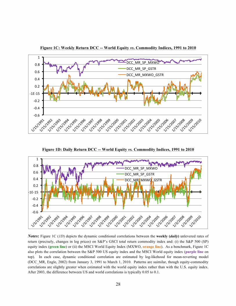
Figure 1C: Weekly Return DCC -- World Equity vs. Commodity Indices, 1991 to 2010

Figure 1D: Daily Return DCC -- World Equity vs. Commodity Indices, 1991 to 2010

Notes: Figure 1C (1D) depicts the dynamic conditional correlations between the weekly (daily) unlevered rates of return (precisely, changes in log prices) on S&P’s GSCI total return commodity index and: (i) the S&P 500 (SP) equity index (green line) or (ii) the MSCI World Equity Index (MXWO, orange line). As a benchmark, Figure 1C also plots the correlation between the S&P 500 US equity index and the MSCI World equity index (purple line on top). In each case, dynamic conditional correlation are estimated by log-likehood for mean-reverting model (DCC_MR, Engle, 2002) from January 3, 1991 to March 1, 2010. Patterns are suimilar, though equity-commodity correlations are slightly greater when estimated with the world equity index rather than with the U.S. equity index. After 2003, the difference between US and world correlations is typically 0.05 to 0.1.

!"#$%

!"#&%

!"#'%

!()!(*%

"#'%

"#&%

"#$%

"#+%

(%,--./0.12./678%

,--./0.12.4150%

,--./0./678.4150%

!"#$%

!"#&%

!"#'%

!()!(*%

"#'%

"#&%

"#$%

"#+%

(%

,--./0.12./678%

,--./0.12.4150%

,--./0./678.4150%

29

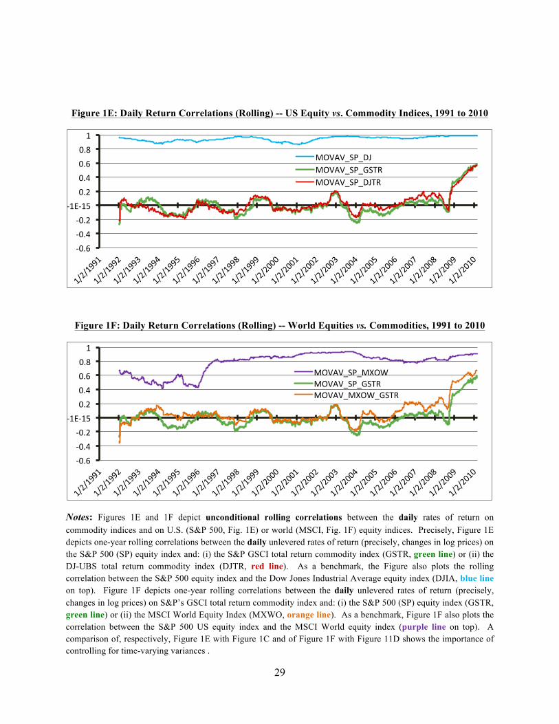
Figure 1E: Daily Return Correlations (Rolling) -- US Equity vs. Commodity Indices, 1991 to 2010

Figure 1F: Daily Return Correlations (Rolling) -- World Equities vs. Commodities, 1991 to 2010

Notes: Figures 1E and 1F depict unconditional rolling correlations between the daily rates of return on commodity indices and on U.S. (S&P 500, Fig. 1E) or world (MSCI, Fig. 1F) equity indices. Precisely, Figure 1E depicts one-year rolling correlations between the daily unlevered rates of return (precisely, changes in log prices) on the S&P 500 (SP) equity index and: (i) the S&P GSCI total return commodity index (GSTR, green line) or (ii) the DJ-UBS total return commodity index (DJTR, red line). As a benchmark, the Figure also plots the rolling correlation between the S&P 500 equity index and the Dow Jones Industrial Average equity index (DJIA, blue line on top). Figure 1F depicts one-year rolling correlations between the daily unlevered rates of return (precisely, changes in log prices) on S&P’s GSCI total return commodity index and: (i) the S&P 500 (SP) equity index (GSTR, green line) or (ii) the MSCI World Equity Index (MXWO, orange line). As a benchmark, Figure 1F also plots the correlation between the S&P 500 US equity index and the MSCI World equity index (purple line on top). A comparison of, respectively, Figure 1E with Figure 1C and of Figure 1F with Figure 11D shows the importance of controlling for time-varying variances .

!"#$%

!"#&%

!"#'%

!()!(*%

"#'%

"#&%

"#$%

"#+%

(%

/89:9.12.,3%/89:9.12.4150%/89:9.12.,350%

!"#$%

!"#&%

!"#'%

!()!(*%

"#'%

"#&%

"#$%

"#+%

(%

/89:9.12./687%/89:9.12.4150%/89:9./687.4150%

30

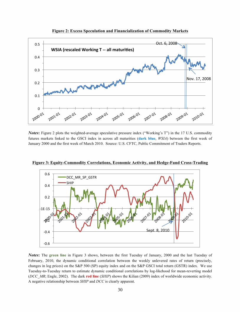
Figure 2: Excess Speculation and Financialization of Commodity Markets

Notes: Figure 2 plots the weighted-average speculative pressure index (“Working’s T”) in the 17 U.S. commodity futures markets linked to the GSCI index in across all maturities (dark blue, WSIA) between the first week of January 2000 and the first week of March 2010. Source: U.S. CFTC, Public Commitment of Traders Reports.

Figure 3: Equity-Commodity Correlations, Economic Activity, and Hedge-Fund Cross-Trading

Notes: The green line in Figure 3 shows, between the first Tuesday of January, 2000 and the last Tuesday of February, 2010, the dynamic conditional correlation between the weekly unlevered rates of return (precisely, changes in log prices) on the S&P 500 (SP) equity index and on the S&P GSCI total return (GSTR) index. We use Tuesday-to-Tuesday return to estimate dynamic conditional correlations by log-likehood for mean-reverting model (DCC_MR; Engle, 2002). The dark red line (SHIP) shows the Kilian (2009) index of worldwide economic activity. A negative relationship between SHIP and DCC is clearly apparent.

"%

"#(%

"#'%

"#;%

"#&%

"#*%!"#$%&'()*+,(-%!.'/012%3%44%+,,%5+67'08()9%

<=>#%(?@%'""+%

8AB#%$@%'""+%

!"#$%

!"#&%

!"#'%

!()!(*%

"#'%

"#&%

"#$%,--./0.12.4150%1CD2%

1EFB#%+@%'"("%

31

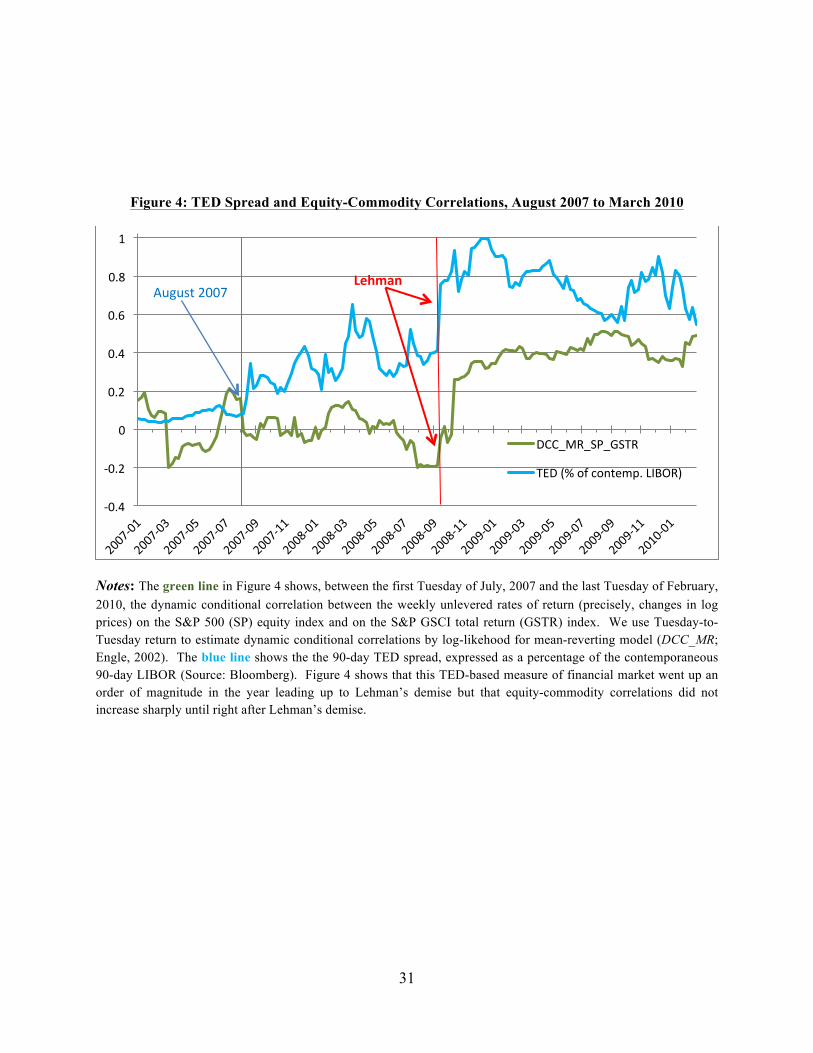
Figure 4: TED Spread and Equity-Commodity Correlations, August 2007 to March 2010

Notes: The green line in Figure 4 shows, between the first Tuesday of July, 2007 and the last Tuesday of February, 2010, the dynamic conditional correlation between the weekly unlevered rates of return (precisely, changes in log prices) on the S&P 500 (SP) equity index and on the S&P GSCI total return (GSTR) index. We use Tuesday-to-Tuesday return to estimate dynamic conditional correlations by log-likehood for mean-reverting model (DCC_MR; Engle, 2002). The blue line shows the the 90-day TED spread, expressed as a percentage of the contemporaneous 90-day LIBOR (Source: Bloomberg). Figure 4 shows that this TED-based measure of financial market went up an order of magnitude in the year leading up to Lehman’s demise but that equity-commodity correlations did not increase sharply until right after Lehman’s demise.

!"#&%

!"#'%

"%

"#'%

"#&%

"#$%

"#+%

(%

,--./0.12.4150%

5),%GH%=I%A=JBEKF#%LDM80N%

:(;5+1%:OPOQB%'""?%

32

Table I: Commodity Weights

!"#$%&'()%*+"#,%

-#./#/%*+"#,% &0$.% 1023"#./% &044""% 156#$% &070#% &0,,0.%

8"#.%+06/%

89:"%7#,,;"%

<""="$%7#,,;"%

>"#,9.6%09;% &$5="%

?#,5$#;%6#/% &0@@"$% A0;=% 19;:"$%

BCCC% !"#$% &"!$% '"($% )"($% &"!$% )"($% ("'$% )")$% !"($% *"&$% ("($% +"*$% '+"'$% ,"*$% +")$% )"($% (")$%BCCD% '"&$% &"'$% '"'$% )"&$% (",$% )")$% ("#$% &"+$% !"&$% *"*$% ("($% *"-$% '+"&$% &("($% *",$% )"&$% (")$%BCCB% '"#$% &"-$% '"+$% )"'$% (",$% &"-$% ("+$% &"*$% )"'$% '",$% (",$% +")$% '-"'$% -"*$% *"*$% )"'$% (")$%BCCE% '"($% &"#$% '"&$% )"#$% ("-$% &"*$% ("#$% &",$% )")$% '")$% &"($% *",$% '-"'$% &&"+$% *"'$% )"&$% (")$%BCCF% !"!$% &"'$% !"*$% )"'$% ("+$% &"!$% ("!$% &"'$% )"&$% !"#$% ("-$% +"+$% #&"*$% &("+$% +"&$% )"($% (")$%BCCG% )"'$% (",$% )"!$% &"*$% ("+$% &"!$% (")$% &"($% &"-$% )"+$% ("+$% -"*$% ##"-$% &&"'$% *"*$% &"+$% (")$%BCCH% )"*$% &"($% )"#$% &"'$% ("+$% &"+$% (")$% (",$% &"#$% )"!$% ("*$% -")$% #*"#$% -"&$% ,"*$% )"($% ("!$%BCCI% !"#$% &")$% !")$% &",$% ("+$% &"&$% (")$% (",$% &"'$% )"*$% ("*$% #",$% #+"&$% +"'$% &("&$% )"($% ("!$%BCCJ% !"-$% (",$% !"*$% )")$% ("*$% &"&$% (")$% ("-$% &"&$% )")$% ("'$% #")$% *&"-$% *",$% *"-$% )"($% (")$%BCCK% '"*$% &"($% '"*$% !")$% (",$% )"($% ("'$% &"($% &",$% !"!$% ("*$% '"!$% ##",$% #"#$% *"-$% !"'$% ("'$%BCDC% '"*$% &"($% '"*$% !")$% (",$% )"($% ("'$% &"($% &",$% !"!$% ("*$% '"!$% ##",$% #"#$% *"-$% !"'$% ("'$%

Note: Table I shows the average weights of the 17 GSCI commodities (out of 24 commodities in the index) for which we have trader position data. We use these weights used to compute the weighted average measures of trader importance (WMSSi and WMSAi, where i=AS, AD, AM, AP, MMT, NRP, etc.) as well as the weighted average speculative index (SIS and SIA). Excluded are four GSCI commodities (aluminum, lead, nickel and zinc) that accounted for less than 5% of the GSCI in 2008 and 2009. The GSCI weight of London Metal Exchange (LME) copper is applied to NYMEX copper positions. Finally, the weight assigned to WTI crude oil is the GSCVI weight of WTI crude, plus the weights of Brent crude, gasoil and RBOB gasoline.

33

Table II: Weekly Rates of Return – Summary Statistics (%, January 1991 to March 2010)

Panel A: S&P 500 Equity Index

1991-2010 1992-1997 1997-2003 2003-2010

Mean 0.124839 0.272260 0.039058 0.049310 Median 0.292318 0.345607 0.366951 0.247137

Maximum 12.37463 4.194317 12.37463 7.818525 Minimum -15.76649 -4.112432 -12.18282 -15.76649 Std. Dev. 2.348732 1.440671 2.943599 2.371901 Skewness -0.596507 -0.258227 -0.026150 -1.440103

Kurtosis 7.920789 3.371816 4.791780 10.70166

Jarque-Bera 1066.091*** 4.42 42.04*** 994.47***

Observations 998 262 314 353

Panel B: S&P GSCI Commodity Index 1991-2010 1992-1997 1997-2003 2003-2010

Mean 0.060691 0.138182 0.044902 0.028993 Median 0.188237 0.148651 0.023027 0.416007

Maximum 14.90087 5.340624 7.479387 14.90087 Minimum -14.59139 -9.208887 -14.59139 -13.12567 Std. Dev. 3.023849 1.811528 2.876870 3.870732 Skewness -0.527095 -0.395102 -0.445674 -0.406732

Kurtosis 5.668868 5.426632 4.888678 4.058999

Jarque-Bera 342.40*** 71.10*** 57.06*** 26.23***

Observations 998 262 314 353 Notes: Table II provides summary statistics for the unlevered rates of return on the S&P 500

equity index (excluding dividends; Panel A), as well as on the S&P GSCI commodity index (total return; Panel B). In each Panel, the first column uses sample moments computed using weekly rates of return (precisely, changes in log prices multiplied by 100) from January 8, 1991 to March 1, 2010. The second, third and fourth columns use, respectively, weekly rates of returns for three successive sub-periods: May 26, 1992 to May 27, 1997; May 27, 1997 to May 27, 2003; and, May 27, 2003 to February 27, 2010. One, two or three stars indicate that normality of the return distribution is rejected at, respectively, the 10%, 5% or 1% level of statistical significance.

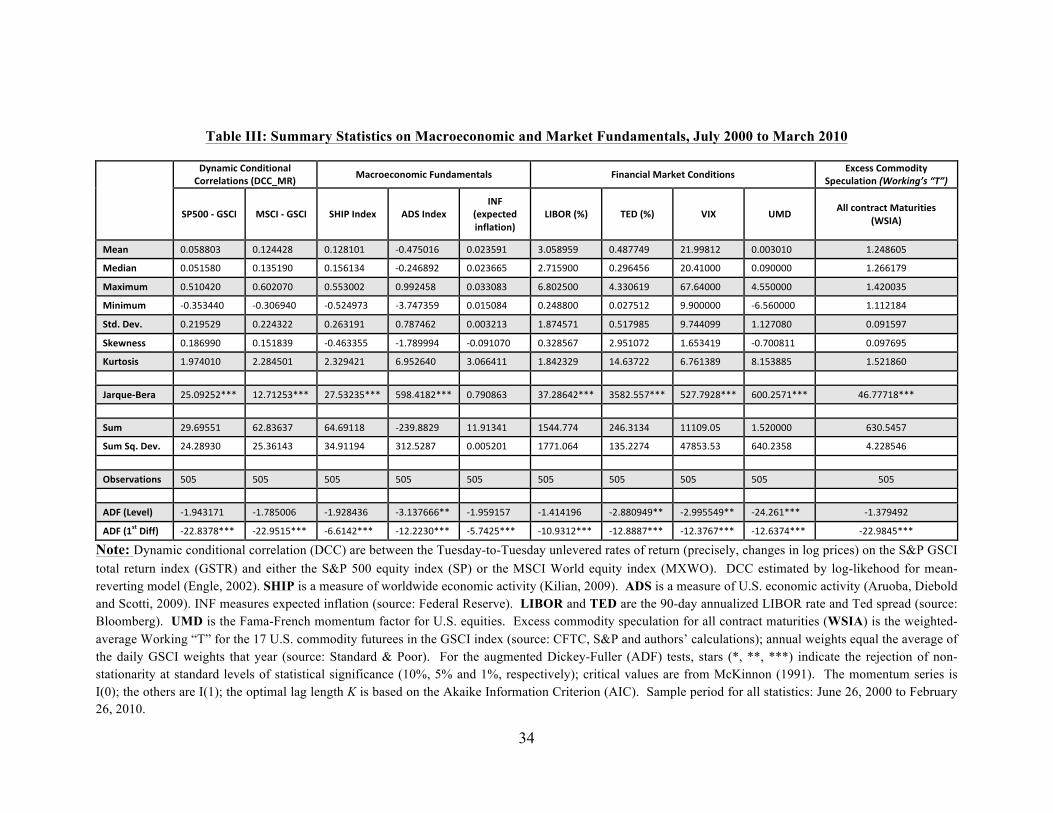
34

Table III: Summary Statistics on Macroeconomic and Market Fundamentals, July 2000 to March 2010

!!!!!!

"#$%&'(!)*$+','*$%-!)*../-%,'*$0!1"))2345! 3%(.*/(*$*&'(!67$+%&/$,%-0! 6'$%$('%-!3%.8/,!)*$+','*$0! 9:(/00!)*&&*+',#!

;</(7-%,'*$!!"#$%&'()*+,-./!

;=>??!@!A;)B! 3;)B!@!A;)B! ;CB=!B$+/:! D";!B$+/:!BE6!

1/:</(,/+!'$F-%,'*$5!

GBHI4!1J5! K9"!1J5! LBM! N3"! D--!(*$,.%(,!3%,7.','/0!1O;BD5!

3/%$! !"!#$$!%& !"'())($& !"'($'!'& *!")+#!',& !"!(%#-'& %"!#$-#-& !")$++)-& ('"--$'(& !"!!%!'!& '"()$,!#&

3/+'%$! !"!#'#$!& !"'%#'-!& !"'#,'%)& *!"(),$-(& !"!(%,,#& ("+'#-!!& !"(-,)#,& (!")'!!!& !"!-!!!!& '"(,,'+-&

3%:'&7&! !"#'!)(!& !",!(!+!& !"##%!!(& !"--()#$& !"!%%!$%& ,"$!(#!!& )"%%!,'-& ,+",)!!!& )"##!!!!& '")(!!%#&

3'$'&7&! *!"%#%))!& *!"%!,-)!& *!"#()-+%& *%"+)+%#-& !"!'#!$)& !"()$$!!& !"!(+#'(& -"-!!!!!& *,"#,!!!!& '"''('$)&

;,+P!"/QP! !"('-#(-& !"(()%((& !"(,%'-'& !"+$+),(& !"!!%('%& '"$+)#+'& !"#'+-$#& -"+))!--& '"'(+!$!& !"!-'#-+&

;8/R$/00! !"'$,--!& !"'#'$%-& *!"),%%##& *'"+$---)& *!"!-'!+!& !"%($#,+& ("-#'!+(& '",#%)'-& *!"+!!$''& !"!-+,-#&

S7.,*0'0! '"-+)!'!& ("($)#!'& ("%(-)('& ,"-#(,)!& %"!,,)''& '"$)(%(-& ')",%+((& ,"+,'%$-& $"'#%$$#& '"#('$,!&! & & & & & & & & & &T%.U7/@H/.%! (#"!-(#(...& '("+'(#%...& (+"#%(%#...& #-$")'$(...& !"+-!$,%& %+"($,)(...& %#$("##+...& #(+"+-($...& ,!!"(#+'...& ),"+++'$...&! & & & & & & & & & &;7&! (-",-##'& ,("$%,%+& ,)",-''$& *(%-"$$(-& ''"-'%)'& '#))"++)& (),"%'%)& '''!-"!#& '"#(!!!!& ,%!"#)#+&

;7&!;UP!"/QP! ()"($-%!& (#"%,')%& %)"-''-)& %'("#($+& !"!!#(!'& '++'"!,)& '%#"((+)& )+$#%"#%& ,)!"(%#$& )"(($#),&! & & & & & & & & & &IV0/.Q%,'*$0! #!#& #!#& #!#& #!#& #!#& #!#& #!#& #!#& #!#& #!#&! & & & & & & & & & &D"6!1G/Q/-5! *'"-)%'+'& *'"+$#!!,& *'"-($)%,& *%"'%+,,,..& *'"-#-'#+& *'")')'-,& *("$$!-)-..& *("--##)-..& *()"(,'...& *'"%+-)-(&

D"6!1W0,!"'FF5! *(("$%+$...& *(("-#'#...& *,",')(...& *'("((%!...& *#"+)(#...& *'!"-%'(...& *'("$$$+...& *'("%+,+...& *'(",%+)...& *(("-$)#...&

Note: Dynamic conditional correlation (DCC) are between the Tuesday-to-Tuesday unlevered rates of return (precisely, changes in log prices) on the S&P GSCI total return index (GSTR) and either the S&P 500 equity index (SP) or the MSCI World equity index (MXWO). DCC estimated by log-likehood for mean-reverting model (Engle, 2002). SHIP is a measure of worldwide economic activity (Kilian, 2009). ADS is a measure of U.S. economic activity (Aruoba, Diebold and Scotti, 2009). INF measures expected inflation (source: Federal Reserve). LIBOR and TED are the 90-day annualized LIBOR rate and Ted spread (source: Bloomberg). UMD is the Fama-French momentum factor for U.S. equities. Excess commodity speculation for all contract maturities (WSIA) is the weighted-average Working “T” for the 17 U.S. commodity futurees in the GSCI index (source: CFTC, S&P and authors’ calculations); annual weights equal the average of the daily GSCI weights that year (source: Standard & Poor). For the augmented Dickey-Fuller (ADF) tests, stars (*, **, ***) indicate the rejection of non-stationarity at standard levels of statistical significance (10%, 5% and 1%, respectively); critical values are from McKinnon (1991). The momentum series is I(0); the others are I(1); the optimal lag length K is based on the Akaike Information Criterion (AIC). Sample period for all statistics: June 26, 2000 to February 26, 2010.

35

Table IV: Simple Correlations, 2000-2010 (Dependent and Explanatory Variables)

&/00123&4516473&&

/00123&289:16473&&

4;<5&& =/4&& ><8&& ?<@:3& 7A/&& <BC& 94<4&& D2/&&

/001231&4516473&& '"!!!!& & & & & & & & & &

/001231&289:16473& !"-#+,...& '"!!!!& & & & & & & & &

4;<5&& *!")),%...& *!"($%-...& '"!!!!& & & & & & & &

=/4&& *!"%!+!...& *!"%($)...& !"%!#$...& '"!!!!& & & & & & &

><8&& !")-',...& !")),)...& *!"#!($...& *!",$##...& '"!!!!& & & & & &

?<@:3&& *!"'$()...& *!"')##...& !"')((...& !"!),)& *!"($-!...& '"!!!!& & & & &

7A/&& !"!$(%.& !"(!$#...& !"'$+,...& *!"##!)...& !"#!%'...& !"(!(,...& '"!!!!& & & &

<BC& *!"'-'(...& *!"($%,...& *!"'+($...& !"%(,%...& *!"%$,-...& !",,-(...& *!"(#$!...& '"!!!!& & &

94<4&& !"'-%!...& !")!+%...& !"#)$$...& *!"(+)+...& !"!,#%& !"!,!#& !"##(#...& *!"#!)%...& '"!!!!& &

D2/&& !"!!%!& *!"!'!'& *!"!)!#& !"!$,-..& *!"!',$& !"!',+& *!"'!)#..& !"!-)-..& *!"!$#(.& '"!!!!&

Note: Table IV shows the simple correlations of the variables in our regression analyses. Stars (*,**,***) highlight correlations that are statistically significantly different from 0 at, respectively, the 10%, 5% and 1% levels of statistical significance. The dependent variables (DCC_MR) are described in the footnote to Figures 1A (SP_GSTR) and 1B (SP_MXWO). The DCC measures are described the footnotes to Table III. Sample period: June 26, 2000 through February 26, 2010.

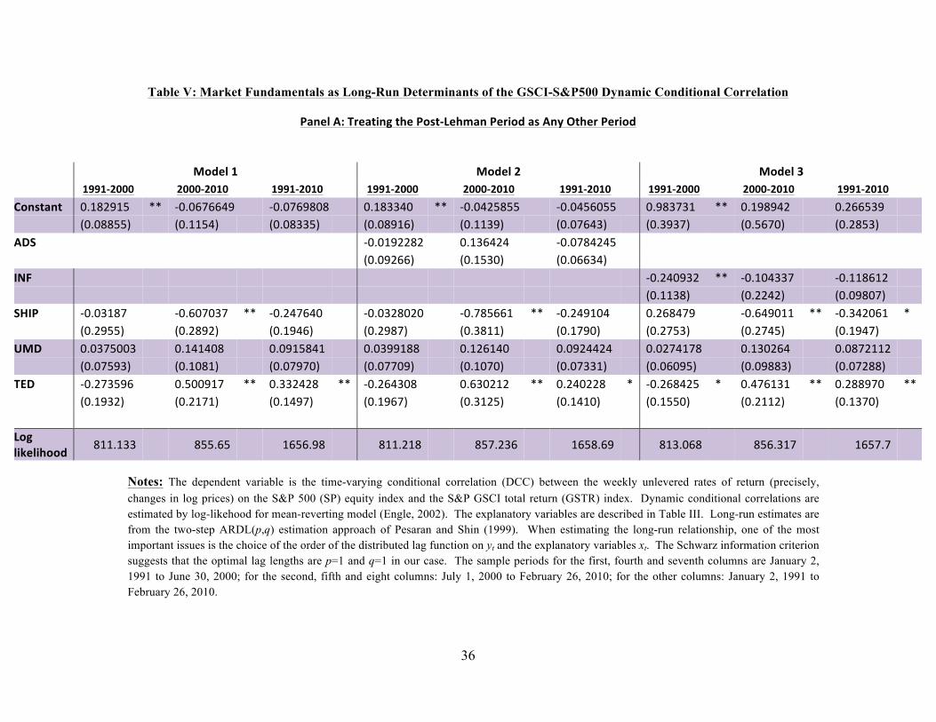
36

Table V: Market Fundamentals as Long-Run Determinants of the GSCI-S&P500 Dynamic Conditional Correlation

=%$/-!DX!K./%,'$Y!,Z/!=*0,@G/Z&%$!=/.'*+!%0!D$#!I,Z/.!=/.'*+!

&

!3*+/-!W! 3*+/-![! 3*+/-!\!

! W]]W@[???! ! [???@[?W?! ! W]]W@[?W?! ! W]]W@[???! ! [???@[?W?! ! W]]W@[?W?! ! W]]W@[???! ! [???@[?W?! ! W]]W@[?W?! !!)*$0,%$,! !"'$(-'#& ..& *!"!,+,,)-& *!"!+,-$!$& !"'$%%)!& ..& *!"!)(#$##& *!"!)#,!##& !"-$%+%'& ..& !"'-$-)(& && !"(,,#%-& &&!! E!"!$$##F& && E!"''#)F& && E!"!$%%#F& && E!"!$-',F& && E!"''%-F& && E!"!+,)%F& && E!"%-%+F& && E!"#,+!F& && E!"($#%F& &&D";!

& & & & &&& *!"!'-(($(& !"'%,)()&

&*!"!+$)()#&

& & & & &&&

! & & & & &&& E!"!-(,,F&

&E!"'#%!F&

&E!"!,,%)F& &&

& & & & &&&

BE6! && && && && && && && && && && && && *!"()!-%(& ..& *!"'!)%%+& && *!"''$,'(& &&!! && && && && && && && && && && && && E!"''%$F& && E!"(()(F& && E!"!-$!+F& &&;CB=! *!"!%'$+&

&*!",!+!%+& ..& *!"()+,)!& && *!"!%($!(!& *!"+$#,,'& ..& *!"()-'!)& && !"(,$)+-&

&*!",)-!''& ..& *!"%)(!,'& .&

!E!"(-##F&

&E!"($-(F&

&E!"'-),F& && E!"(-$+F&

&E!"%$''F&

&E!"'+-!F& && E!"(+#%F&

&E!"(+)#F&

&E!"'-)+F& &&

N3"! !"!%+#!!%& && !"')')!$& && !"!-'#$)'& && !"!%--'$$& && !"'(,')!& && !"!-())()& && !"!(+)'+$& && !"'%!(,)& && !"!$+(''(& &&!! E!"!+#-%F& && E!"'!$'F& && E!"!+-+!F& && E!"!++!-F& && E!"'!+!F& && E!"!+%%'F& && E!"!,!-#F& && E!"!-$$%F& && E!"!+($$F& &&K9"! *!"(+%#-,&

&!"#!!-'+& ..& !"%%()($& ..& *!"(,)%!$&

&!",%!('(& ..& !"()!(($& .& *!"(,$)(#& .& !")+,'%'& ..& !"($$-+!& ..&

!E!"'-%(F&

&E!"('+'F&

&E!"')-+F& && E!"'-,+F&

&E!"%'(#F&

&E!"')'!F& && E!"'##!F&

&E!"(''(F&

&E!"'%+!F& &&

!&&

& & & &&& &&

& & & &&& &&

& & & &&&

G*Y!-'8/-'Z**+! $''"'%%& && $##",#& && ',#,"-$& && $''"('$& && $#+"(%,& && ',#$",-& && $'%"!,$& && $#,"%'+& && ',#+"+& &&

&

Notes: The dependent variable is the time-varying conditional correlation (DCC) between the weekly unlevered rates of return (precisely, changes in log prices) on the S&P 500 (SP) equity index and the S&P GSCI total return (GSTR) index. Dynamic conditional correlations are estimated by log-likehood for mean-reverting model (Engle, 2002). The explanatory variables are described in Table III. Long-run estimates are from the two-step ARDL(p,q) estimation approach of Pesaran and Shin (1999). When estimating the long-run relationship, one of the most important issues is the choice of the order of the distributed lag function on yt and the explanatory variables xt. The Schwarz information criterion suggests that the optimal lag lengths are p=1 and q=1 in our case. The sample periods for the first, fourth and seventh columns are January 2, 1991 to June 30, 2000; for the second, fifth and eight columns: July 1, 2000 to February 26, 2010; for the other columns: January 2, 1991 to February 26, 2010.

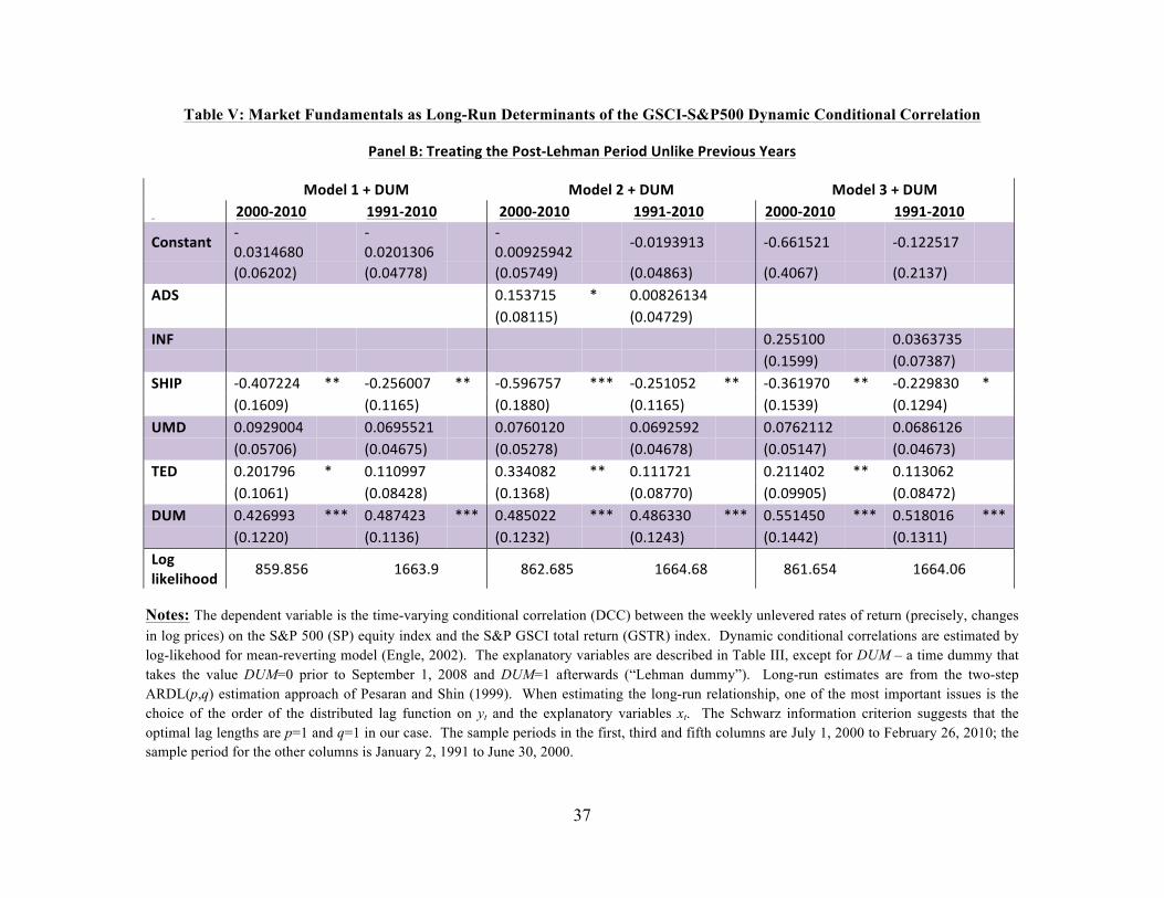
37

Table V: Market Fundamentals as Long-Run Determinants of the GSCI-S&P500 Dynamic Conditional Correlation

=%$/-!HX!K./%,'$Y!,Z/!=*0,@G/Z&%$!=/.'*+!N$-'8/!=./Q'*70!^/%.0!

!! 3*+/-!W!_!"N3! 3*+/-![!_!"N3! 3*+/-!\!_!"N3!!! [???@[?W?!

!W]]W@[?W?!

![???@[?W?!

!W]]W@[?W?!

![???@[?W?!

!W]]W@[?W?!

!)*$0,%$,! *

!"!%'),$!& && *!"!(!'%!,& && *

!"!!-(#-)(& && *!"!'-%-'%& && *!",,'#('& && *!"'((#'+& &&

!! E!"!,(!(F& && E!"!)++$F& && E!"!#+)-F& && E!"!)$,%F& && E!")!,+F& && E!"('%+F& &&D";!

& & & &!"'#%+'#& .& !"!!$(,'%)&

& & & &&&

!!& & & &

E!"!$''#F&&

E!"!)+(-F&& & & &

&&BE6!

& & &&&

& & &&& !"(##'!!& && !"!%,%+%#& &&

!!& & &

&&& & &

&& E!"'#--F& && E!"!+%$+F& &&;CB=! *!")!+(()& ..& *!"(#,!!+& ..& *!"#-,+#+& ...& *!"(#'!#(& ..& *!"%,'-+!& ..& *!"((-$%!& .&!! E!"',!-F&

&E!"'',#F&

&E!"'$$!F&

&E!"'',#F&

&E!"'#%-F&

&E!"'(-)F& &&

N3"! !"!-(-!!)& && !"!,-##('& && !"!+,!'(!& && !"!,-(#-(& && !"!+,(''(& && !"!,$,'(,& &&!! E!"!#+!,F& && E!"!),+#F& && E!"!#(+$F& && E!"!),+$F& && E!"!#')+F& && E!"!),+%F& &&K9"! !"(!'+-,& .& !"''!--+&

&!"%%)!$(& ..& !"'''+('&

&!"('')!(& ..& !"''%!,(& &&

!! E!"'!,'F&&

E!"!$)($F&&

E!"'%,$F&&

E!"!$++!F&&

E!"!--!#F&&

E!"!$)+(F& &&"N3! !")(,--%& ...& !")$+)(%& ...& !")$#!((& ...& !")$,%%!& ...& !"##')#!& ...& !"#'$!',& ...&!! E!"'((!F& && E!"''%,F& && E!"'(%(F& && E!"'()%F& && E!"'))(F& && E!"'%''F& &&G*Y!-'8/-'Z**+! $#-"$#,& && ',,%"-& && $,(",$#& && ',,)",$& && $,'",#)& && ',,)"!,& &&

!

Notes: The dependent variable is the time-varying conditional correlation (DCC) between the weekly unlevered rates of return (precisely, changes in log prices) on the S&P 500 (SP) equity index and the S&P GSCI total return (GSTR) index. Dynamic conditional correlations are estimated by log-likehood for mean-reverting model (Engle, 2002). The explanatory variables are described in Table III, except for DUM – a time dummy that takes the value DUM=0 prior to September 1, 2008 and DUM=1 afterwards (“Lehman dummy”). Long-run estimates are from the two-step ARDL(p,q) estimation approach of Pesaran and Shin (1999). When estimating the long-run relationship, one of the most important issues is the choice of the order of the distributed lag function on yt and the explanatory variables xt. The Schwarz information criterion suggests that the optimal lag lengths are p=1 and q=1 in our case. The sample periods in the first, third and fifth columns are July 1, 2000 to February 26, 2010; the sample period for the other columns is January 2, 1991 to June 30, 2000.

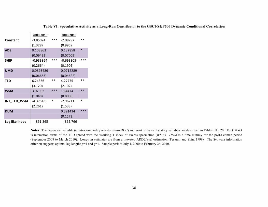
38

Table VI: Speculative Activity as a Long-Run Contributor to the GSCI-S&P500 Dynamic Conditional Correlation

!! [???@[?W?! ! [???@[?W?! !)*$0,%$,! *%"$#!()& ...& *("!$+-+& ..&!! E'"%($F&

&E!"--#-F&

&D";! !"'!%$,%& && !"'%($#$& .&!! E!"!-)-(F& && E!"!+!!-F& &&;CB=! *!"-%%$,)& ...& *!",-%$!#& ...&!! E!"(,,)F&

&E!"'-!#F&

&N3"! !"!$-%)$,& && !"!+'(($-& &&!! E!"!,,#%F& && E!"!),((F& &&K9"! ,"()%,,& ..& )"(+++#& ..&!! E%"'(!F&

&E("'!(F&

&O;BD! %"!+%!(& ...& '",))+)& ..&!! E'"!)$F&

&E!"$!!$F&

&BEK2K9"2O;BD! *)"%+#)%& .& *("-,+''& .&!! E("(,'F&

&E'"#%%F&

&"N3!

& &!"%-')%)& ...&

!!& &

E!"'(+%F& &&G*Y!-'8/-'Z**+! $,'"%,#& && $,#"+,,& &&

Notes: The dependent variable (equity-commodity weekly return DCC) and most of the explanatory variables are described in Tables III. INT_TED_WSIA is interaction terms of the TED spread with the Working T index of excess speculation (WSIA). DUM is a time dummy for the post-Lehman period (September 2008 to March 2010). Long-run estimates are from a two-step ARDL(p,q) estimation (Pesaran and Shin, 1999). The Schwarz information criterion suggests optimal lag lengths p=1 and q=1. Sample period: July 1, 2000 to February 26, 2010.