speculation, trading and bubbles

Speculation,trading and

bubbles

Jose A.Scheinkman

Introduction

Stylized Facts

Model

Remark onleverage

Additionalevidence

References

Speculation, trading and bubbles

Jose A. Scheinkman∗

∗Columbia University and NBER

CUNYSeptember, 2013

0/49


bubbles

Jose A.Scheinkman

Introduction

Stylized Facts

Model

Remark onleverage

Additionalevidence

References

Plan I

1 Discuss some stylized facts concerning bubbles.

2 Present a very simple model for bubbles and argue that itfits these facts.

• Distillation of some previous work with Hong, Xiong.

3 Make a remark on leverage.

4 Present some additional evidence

1/49


bubbles

Jose A.Scheinkman

Introduction

Stylized Facts

Model

Remark onleverage

Additionalevidence

References

Stylized facts a theory of bubblesshould accommodate I

1 Asset price bubbles coincide with increases in tradingvolume.

2 Asset price bubble implosions often coincide with increasesin asset supply.

• shorting

• Asset price bubbles often coincide with financial ortechnological innovations.

2/49


bubbles

Jose A.Scheinkman

Introduction

Stylized Facts

Model

Remark onleverage

Additionalevidence

References

Bubbles and trading volume:South Sea Bubble I

• Extraordinary rise and fall of price of South Sea Companyshares and other similar joint-stock companies in 1720.

• ∼ 2,000 transactions per year in Bank of England stock1717-1719, 6,846 transactions (100% of stocksoutstanding) in 1720.

• East India Company and Royal African Company turnedover 150% of stock outstanding in 1720.

• Carlos et al. (2006)

3/49


bubbles

Jose A.Scheinkman

Introduction

Stylized Facts

Model

Remark onleverage

Additionalevidence

References

Bubbles and trading volume:Roaring Twenties I

• Accounts of stock-market boom of late 1920s emphasizeovertrading in 28-29.

• Annual turnover at NYSE climbs from 100% per annum in1925-27 to over 140% in 1928 and 1929. Davis et al.(2005)

• All-time daily records of share trading volume werereached 10 times in 1928 and 3 times in 1929. New recordnot set until April 1, 1968, when LBJ announced he wouldnot seek re-election (Hong and Stein (2007))

4/49


bubbles

Jose A.Scheinkman

Introduction

Stylized Facts

Model

Remark onleverage

Additionalevidence

References

Bubbles and trading volume:Internet... I

• During the DotCom bubble internet stocks had 3 timesthe turnover of other similar stocks.

• Lamont and Thaler (2003): 6 cases of spinoffs average38% daily turnover.

• Typical NYSE stock turnover of 100% per year.

• Cochrane (2002) documents cross sectional correlationbetween a stock’s market/book and that stock’s turnover.

• China’s A& B shares - Correlation between higher A-Bpremium and volume in panel. (Mei et al. (2009))

5/49


bubbles

Jose A.Scheinkman

Introduction

Stylized Facts

Model

Remark onleverage

Additionalevidence

References

Bubble implosion and supply I

• In 1720, new issues by the South Sea Company doubledthe amount of shares outstanding.

• Outstanding shares of the Royal African Company morethan tripled.

• Numerous other joint-stock companies started (Bubbles).

• Bubble Act of 1720: Parliament banned joint-stockcompanies not authorized by Royal Charter or theextension of corporate charters into new ventures.

• “the [Bubble Act] was a special-interest legislation for the[South-Sea Company], which controlled its framing and itspassage” (Harris (1994))

• Bubble act used by South Sea Company to sue oldchartered companies that had changed activities and whereattracting speculators.

6/49


bubbles

Jose A.Scheinkman

Introduction

Stylized Facts

Model

Remark onleverage

Additionalevidence

References

Bubble implosion and supply II

• Extraordinary number of lock up expirations for DotComcompanies in H1 2000. (Ofek and Richardson (2003))

• Venture capital firms that had distributed 3.9 billion tolimited partners in third quarter of 1999, distributed 21billion in 2000 Q1. (Janeway (2012))

• Regulatory innovation (CDS on CDOs), and financialengineering (ABX index, synthetic Collateralized DebtObligation (CDO)) increased supply of “safe” securitiesand led to the implosion of the credit bubble.

7/49


bubbles

Jose A.Scheinkman

Introduction

Stylized Facts

Model

Remark onleverage

Additionalevidence

References

Bubbles: definition(s) I

1 Asset prices exceed an asset’s fundamental value

2 Asset prices exceed fundamentals because owners believethey can resell the asset for a higher price in the future.(Brunnermeier (2008))

8/49


bubbles

Jose A.Scheinkman

Introduction

Stylized Facts

Model

Remark onleverage

Additionalevidence

References

Bubbles: Theories I

• Rational Bubbles (Tirole (1985), Santos and Woodford(1997))

• Prices exceed fundamental value because they are expectedto exceed fundamental value by even more tomorrow.

• Difficulty dealing with finite-lived assets.• Do not generate correlation with trading volume.

• A positive shock is amplified by extrapolation of pastreturns (Shiller (2006))

• Getting association with trading volume requires a linkbetween extrapolation and disagreement.

• Limited arbitrage• Asymmetry between costs of going short vs. long.• Heterogeneous beliefs (Miller, 1977;Harrison and Kreps

(1978).)• Absence of common knowledge that bubble exists (Allen

et al. (1993); Abreu and Brunnermeier (2003).)

9/49


bubbles

Jose A.Scheinkman

Introduction

Stylized Facts

Model

Remark onleverage

Additionalevidence

References

Principal assumptions I

• Costly shorting

• Heterogeneous beliefs from overconfidence, the tendencyof people to overestimate the precision of their knowledge.

• Disciplining device

• Certainly not the only mechanisms that cause bubbles inreality.

• Far from being standard in economics• Economic models typically assume symmetric costs

between going long and going short• Results showing that rational investors with common priors

cannot agree to disagree.• No trade theorems (Milgrom, Stokey, Tirole): Unless some

traders trade for “irrational” reasons, there is no trade.

10/49


bubbles

Jose A.Scheinkman

Introduction

Stylized Facts

Model

Remark onleverage

Additionalevidence

References

Evidence for costly short-sale I

• Some obvious cases

• Housing• CDO’s before the introduction of ABX and synthetic

CDO’s.

• Shorting mechanisms for stocks (D’avolio (2002))

• Stocks with higher dispersion of earnings forecasts havelower future returns (Diether et al. (2002))

• It is easier for optimists to express their beliefs in markets.

11/49


bubbles

Jose A.Scheinkman

Introduction

Stylized Facts

Model

Remark onleverage

Additionalevidence

References

Evidence of overconfidence I

• Alpert and Raiffa (1982).

• Documented among: Engineers (Kidd (1970)),Entrepreneurs (Cooper et al. (1988))...

• Ben-David et al. (2010) on CFO predictions of S&Preturns.

• Realized returns are within executives [10%,90%] intervals33% of the time.

12/49


bubbles

Jose A.Scheinkman

Introduction

Stylized Facts

Model

Remark onleverage

Additionalevidence

References

A sketch of a model I

• With Hong, Xiong

• Very simplified version

• Investors in model estimate the “state” of the systemusing signals they believe are related to that state.

• Filtering.

• Investors have heterogeneous beliefs• Some investors attribute excessive informativeness to

certain (volatile) signals. Others may be rational• Group A is “rational” but group B thinks that opinion of a

business commentator correlates well with future dividends.• Overconfidence (miscalibration): Some investors

overestimate how much they know .• No learning about overconfidence (horizon).• Investors know relative opinions fluctuate.

13/49


bubbles

Jose A.Scheinkman

Introduction

Stylized Facts

Model

Remark onleverage

Additionalevidence

References

A sketch of a model I

• Buyers know that in the future optimists may be willing topay more than their own reservation value.

• Short sales are costly

• Optimists have an easier time expressing their opinions.

• Bubble = value of resale option. (cf. definition)

• Conservative measure

14/49


bubbles

Jose A.Scheinkman

Introduction

Stylized Facts

Model

Remark onleverage

Additionalevidence

References

Consequences I

• A higher degree of overconfidence leads to higher pricesand a higher value for the resale option.

• Also leads to more volatile relative opinions and thushigher trading volume.

• Lower borrowing costs make resale option more valuable.

• Shorter horizon implies fewer opportunities to resell, thussmaller bubble.

• When investors have limited capacity to bear risk, anincrease in the supply of the asset is absorbed by lessoptimistic buyers.

• Valuation that marginal buyer has of the future payoffsdeclines as supply increases.

• Lower discounted fundamental value of the asset.

15/49


bubbles

Jose A.Scheinkman

Introduction

Stylized Facts

Model

Remark onleverage

Additionalevidence

References

Consequences II

• Buyer also knows that because the larger supply needs tobe absorbed, future marginal buyers are likely to be lessoptimistic and thus the value of the resale option declines.

• Increase in asset supply diminishes (deflates) thebubble.

• Shorting

• Leverage.

16/49


bubbles

Jose A.Scheinkman

Introduction

Stylized Facts

Model

Remark onleverage

Additionalevidence

References

A simple model I

• 4 periods t = 1, 2, 3, 4, a single good, and single riskyasset in finite supply S .

• Risk-free technology. An investment of δ units of the goodin any period t yields one unit in period t + 1.

• Large number of risk-neutral investors, that only valueconsumption in the final period t = 4.

• Risky asset produces dividend θt at t = 2, 3, 4.

• θt ∈ {θ`, θh} with θh > θ`, is independent of the past andfuture dividends and Prob[θt = θ`] = .5

•θ = E(θt) = .5θ` + .5θh.

• No short-sales, no borrowing.

• Assets traded at t = 1, 2, 3, 4, ex-dividend.

• p4 = 0.

17/49


bubbles

Jose A.Scheinkman

Introduction

Stylized Facts

Model

Remark onleverage

Additionalevidence

References

A simple model: Signals I

• Signal st at t = 1, 2, 3 observed before trading occurs at t,but after the dividend at t (if t > 1) is observed.

• st ∈ {0, 1, 2}, has no predictive power for future dividends.

• Two sets of investors, A and B, each with many investors.

• Agents in A are rational.

• Agents in B actually believe that st predicts θt+1:

Prob[θt+1 = θh|st ] = .5 + g(st − 1), 0 < g < .5.

• A and B agree st is i .i .d and does not predict θt+j , j ≥ 2

• Prob[st = 0] = Prob[st = 2] = q ≤ .5

• Ex-ante no optimism or pessimism.

• Precision inverse of variance. B ′s have exaggerated viewof the precision of their beliefs when st ∈ {0, 2}.

18/49


bubbles

Jose A.Scheinkman

Introduction

Stylized Facts

Model

Remark onleverage

Additionalevidence

References

A simple model: no capitalconstraints I

• vCt willingness to pay of member of group C ∈ {A, B} for

an infinitesimal amount of the risky asset.

•vCt = δ

[EC (θt+1|st) + E(pt+1)

]

19/49


bubbles

Jose A.Scheinkman

Introduction

Stylized Facts

Model

Remark onleverage

Additionalevidence

References

A simple model: no capitalconstraints II

st Buyer p3 p2

0 A δθ δ(θ + Ep3)1 A, B δθ δ(θ + Ep3)2 B δ[θ + g(θh − θ`)] δ(θ + g(θh − θl ) + Ep3)Ep − δ[θ + qg(θh − θ`)] (δ + δ2)[θ + qg(θh − θ`)]Bubble − 0 δ2qg(θh − θ`)

st Buyer p1

0 A δ(θ + Ep2)1 A, B δ(θ + Ep2)2 B δ(θ + g(θh − θl ) + Ep2)Ep − . . .Bubble − (δ2 + δ3)qg(θh − θ`)

20/49


bubbles

Jose A.Scheinkman

Introduction

Stylized Facts

Model

Remark onleverage

Additionalevidence

References

Volume of trade I

•EV1 =

1

2× 2q × S = qS .

• Trade in period 2 if history (2,0) or (0,2) occurs. Also(1,2) and (1,0) but only half the volume.

EV2 = 2q2S + (1− 2q)2q × S

2= qS .

• Similarly EV3 = qS .

21/49


bubbles

Jose A.Scheinkman

Introduction

Stylized Facts

Model

Remark onleverage

Additionalevidence

References

Summary of results I

Proposition

In the presence of fluctuating differences in beliefs andshort-sale constraints, bubble exists - investors are willing topay for an asset in excess of their own valuation of futuredividends. In addition,

(i) Bubble increases when the probability of disagreementincreases.

(ii) Volume of trade increases with the probability ofdisagreement.

(iii) Size of the bubble decreases with the risk-free interestrate.

(iv) The bubble declines as the time to maturity of the assetapproaches, because there are fewer opportunities totrade.

22/49


bubbles

Jose A.Scheinkman

Introduction

Stylized Facts

Model

Remark onleverage

Additionalevidence

References

Limited Capital I

• Group A has enough capital to acquire full supply at theirreservation price vA

t . Group B has limited capital.

• The introduction of agents with limited capital can onlylower vC

t

• St for the total supply of the asset, KCt the capital

available for purchases for agents in group C , at t.

• AssumeKA

t

St − SAt−1

> vAt (1)

• If vAt ≥ vB

t then the price of the asset pt = vAt .

• If KBt

(St−SBt−1)≥ vB

t > vAt then pt = vB

t .

23/49


bubbles

Jose A.Scheinkman

Introduction

Stylized Facts

Model

Remark onleverage

Additionalevidence

References

Limited Capital II

• If vAt ≤

KBt

(St−SBt−1)

< vBt , then

pt =KB

t

(St − SBt−1)

.

• Cash-in-the-market-pricing, Allen and Gale (2002).

• If vAt > KB

t

(St−SBt−1)

then pt = vAt .

•

pt = max

{vAt , min

{vBt ,

KBt

(St − SBt−1)

}}• Other things equal, this price decreases as St increases.

• If float is large enough, then even when B agents areoptimists some of the asset supply ends up in the hands ofA agents, because of the limited capital of group B agents.

24/49


bubbles

Jose A.Scheinkman

Introduction

Stylized Facts

Model

Remark onleverage

Additionalevidence

References

Limited Capital III

• Larger float lowers the price and the turnover of the asset.

• If the supply of risky asset remains constant through time,a larger float is associated with smaller turnover.

25/49


bubbles

Jose A.Scheinkman

Introduction

Stylized Facts

Model

Remark onleverage

Additionalevidence

References

Change in Float I

• Buyer’s of the stock of the South Sea Company or buyersof Internet stocks in the late 90’s did not know withcertainty the future supply of these assets.

• S0 = S1 = S and S3 = S2 = S with probability π andS + ∆S > S with probability 1− π.

• Realization of the supply of the risky asset is independentof the realization of (θ1, θ2, s1, s2), and observed in period2 before the signal s2 is observed.

• Investors know the supply when they trade in period 2.

• Increase in supply will come from sales of the asset by“insiders”, as in Hong et al. (2006).

• To simplify matters assume that insiders only wish to sell.

26/49


bubbles

Jose A.Scheinkman

Introduction

Stylized Facts

Model

Remark onleverage

Additionalevidence

References

Bubble implosion I• Will show that for certain parameter values, bubble exists

for t < 2 and persists if S2 = S but deflates when thesupply increases.

• Start by imposing bounds on the aggregate portfolio ofgroup B agents that will insure that the bubble persistswhen the supply of the asset is unchanged and the bubbledeflates when the supply increases

• Later show that these bounds would hold when the initialsupply S is sufficiently small and the potential increase inthe supply in period 2, ∆S , is sufficiently large.

• Assume

KB3

S − SB2

≥ δ[θ + g(θh − θ`)], (2)

KB3

S + ∆S − SB2

< δθ. (3)

27/49


bubbles

Jose A.Scheinkman

Introduction

Stylized Facts

Model

Remark onleverage

Additionalevidence

References

Bubble implosion II• Equivalently could assume reservation price of insiders

> vB2 , with probability π, and < δθ, otherwise.

• Given (2) and (3) insiders sell no shares with probability πand sell all their shares with probability 1− π.

• When S2 = S , p3 matches the price with no capitalconstraints whereas when S2 = S + ∆S , p3 = vA

3 .

• If S2 = S + ∆S , no period 2 bubble, since it is known thatperiod 3 prices are independent of signal s3.

• if S2 = SEp3 = δ[θ + qg(θh − θ`)],

since B agents acquire the whole float if s3 = 2.

• To insure that if S2 = S , p2 = price no constraints,

KB2

S − SB1

≥ (δ + δ2)[θ + qg(θh − θ`)]. (4)

28/49


bubbles

Jose A.Scheinkman

Introduction

Stylized Facts

Model

Remark onleverage

Additionalevidence

References

Bubble implosion III

• To insure that when S2 = S + ∆S , the marginal buyer ofthe asset in period 2 always belongs to A, it suffices that

KB2

S + ∆S − SB1

≤ (δ + δ2)θ. (5)

• If inequalities (2) - (5) hold then before S2 (and hence s2)is observed

Ep2 = (δ + δ2)[θ + qπg(θh − θ`)]

• If inequalities (2), (3) and (4) hold, rational buyers inperiod 1 will always be willing to pay in excess of their ownvaluations of future dividends of the risky asset, because ifsupply does not increase they may have an opportunity tosell the asset to over-optimistic B agents in the future.

29/49


bubbles

Jose A.Scheinkman

Introduction

Stylized Facts

Model

Remark onleverage

Additionalevidence

References

Bubble implosion IV

• Since A agents have sufficient capital to buy the totalsupply of the asset at these higher prices, the price of theasset in period 1 exceeds the expected discounteddividends independently of the realized signal in period 1(s1) and the capital constraints of group B agents.

• When s1 = 2,

vB1 (2) = δ

(θ + qg(θh − θ`) + (δ + δ2)[θ + qπg(θh − θ`)]

),

which exceeds the present value of dividends expected bygroup B agents by (δ + δ2)[qπg(θh − θ`)].

• To guarantee that when s1 = 2, p1 = vB1 (2) one must

assume that:KB

1

S − SB0

≥ vB1 (2) (6)

30/49


bubbles

Jose A.Scheinkman

Introduction

Stylized Facts

Model

Remark onleverage

Additionalevidence

References

Bubble implosion V

• In this case b1 = (δ2 + δ3)πqg(θh − θ`),

• Smaller than the bubble that obtains when liquidityconstraints are not binding - reflecting the possibility thatfuture supplies may increase.

• Inequalities (2), (4) and (6) hold provided S is smallenough (relative to wealth of group B agents)

• Inequalities (3) and (5) hold provided ∆S is large enough(relative to initial wealth of group B agents.)

• Showing this amounts to examining evolution of wealth inequilibrium. (see Appendix)

• Bubble arises if initial supply is small relative to optimistscapital and there is a chance that supply will not increaseand implodes if there is a realization of a large supply.

• Supply

31/49


bubbles

Jose A.Scheinkman

Introduction

Stylized Facts

Model

Remark onleverage

Additionalevidence

References

Bubble implosion VI

• Shorting

• Leverage (how much wealth is available to B’s).

32/49


bubbles

Jose A.Scheinkman

Introduction

Stylized Facts

Model

Remark onleverage

Additionalevidence

References

Leverage I

• Loans from pessimists to optimists, Geanakoplos (2010)

• For tax or regulatory reasons, not all optimists are theadequate holders of certain risky assets.

• Although not the most appropriate direct investors inhouses, optimistic banks could make loans charging morethan prime rates to subprime buyers that would be capableof repaying their loans in the “likely” event that houseprices continued to behave as in the previous ten years.

• Foote et al. (2012)• A money market fund that was willing to finance 98.4% of

the purchase-price of a AAA mortgage security to aninvestor in 2006 probably thought that these securitieswere actually nearly risk-free, warranting a leverage of 60.

• Landesbanks

33/49


bubbles

Jose A.Scheinkman

Introduction

Stylized Facts

Model

Remark onleverage

Additionalevidence

References

Leverage II• Two periods t = 0, 1.

• Two non-storable consumption goods.

• Single asset that pays in period 1, x ∈ {κ, K} units of theperiod 1 good, with 0 < κ << K .

• Three groups of same size A, B, N, of risk-neutral agentswith utility function

c0 + δ[πC c1(K ) +

(1− πC

)c1(κ)

]for C ∈ (A, B, N).

• πN ≥ πB > πA.

• Agents in group N are not allowed to purchase asset.

• Asset in inelastic supply =1 from agents outside model.

• Agent in group C has endowment W C of the good inperiod 0 and endowment 0 of the period 1 good.

34/49


bubbles

Jose A.Scheinkman

Introduction

Stylized Facts

Model

Remark onleverage

Additionalevidence

References

Leverage III

• Collateralized loans. Loan of s units of 0-good in exchangefor promise (y1, y2) collateralized by 1 unit of the asset. Tobe credible, y1 ≤ κ and y2 ≤ K . Contract C = (s, y1, y2).

• High leverage requires y1 > y2 and since πA < πB

leverage by A’s is expensive for B’s.

• Suppose A′s lend to B ′s using a contract C. If y2 > y1,N ′s value payoff more than A′s. In equilibrium no loansfrom A’s, unless N’s exhaust their capital.

• Thus if N ′s have enough capital, any contract involvingA′s must have y2 ≤ y1 ≤ κ. (riskless, low leverage)

• In this example, if N ′s have sufficient capital, p can exceedthe valuation of B’s.

• Leverage as a result of (successful) attempt to circumventregulation.

35/49


bubbles

Jose A.Scheinkman

Introduction

Stylized Facts

Model

Remark onleverage

Additionalevidence

References

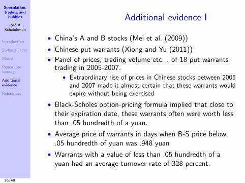
Additional evidence I

• China’s A and B stocks (Mei et al. (2009))

• Chinese put warrants (Xiong and Yu (2011))

• Panel of prices, trading volume etc... of 18 put warrantstrading in 2005-2007.

• Extraordinary rise of prices in Chinese stocks between 2005and 2007 made it almost certain that these warrants wouldexpire without being exercised

• Black-Scholes option-pricing formula implied that close totheir expiration date, these warrants often were worth lessthan .05 hundredth of a yuan.

• Average price of warrants in days when B-S price below.05 hundredth of yuan was .948 yuan

• Warrants with a value of less than .05 hundredth of ayuan had an average turnover rate of 328 percent.

36/49


bubbles

Jose A.Scheinkman

Introduction

Stylized Facts

Model

Remark onleverage

Additionalevidence

References

Additional evidence II• On last trading day, virtually worthless, warrants turned,

on average, over 100% of their float every 20 minutes!

• Larger float of a warrant associated with smaller bubble.

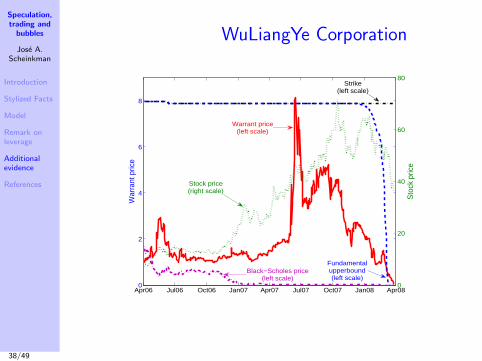
• Put warrant on the stock of WuLiangYe Corporation, aliquor producer

• Warrant issued on April 3, 2006 in-the-money with anexercise price of 7.95 yuan while WuLiangYe’s stock tradedat 7.11 yuan.

• In October 15th 2007, stock reached peak of 71.56 yuanand then drifted down to close at 26 yuan at expiration.

• Calculations by Xiong and Yu (2011) is that after July 07,the Black-Scholes price of this put was below .05hundredth of a yuan, but the warrant traded for a fewyuans, and only dropped below its initial price of .99 yuanin the last few trading days.

• Warrant on the stock of WuLiangYe Corporation volume oftrade on the last trading day was 1,841%.

37/49


bubbles

Jose A.Scheinkman

Introduction

Stylized Facts

Model

Remark onleverage

Additionalevidence

References

WuLiangYe Corporation

12

Figure 1. Prices of WuLiang put warrant

This figure shows the daily closing prices of WuLiang stock and its put warrant, along with WuLiang warrant's strike price, upper bound of its fundamental value assuming WuLiang stock price drops 10 percent every day before expiration (maximum allowed per day in China’s stock market), and its Black-Scholes price using WuLiang stock’s previous one-year rolling daily return volatility.

Apr06 Jul06 Oct06 Jan07 Apr07 Jul07 Oct07 Jan08 Apr080

2

4

6

8

War

rant

pric

e

0

20

40

60

80

Sto

ck p

rice

Strike(left scale)

Stock price(right scale)

Fundamentalupperbound(left scale)

Warrant price(left scale)

Black−Scholes price(left scale)

Figure 1 plots the daily closing prices of WuLiang stock and the put warrant during its

lifetime. The WuLiang stock had a stock split of 1 to 1.402 during the life of the warrant. As the

warrant is adjusted for the stock split and dividend payouts, Figure 1 is based on the pre-split

share unit, but adjusts for dividend payout. For consistency, we use pre-split share unit

throughout our discussion of the WuLiang warrant in this section. The WuLiang stock price

increased from 7.11 Yuan on April 3, 2006 to a peak of 71.56 Yuan on October 15, 2007, and

then retreated to around 26 Yuan when the warrant expired. While the put warrant was initially

issued in the money, the big run up of WuLiang stock price soon pushed the warrant out of

money after two weeks, and it never came back in the money. Despite this, the warrant price

38/49


bubbles

Jose A.Scheinkman

Introduction

Stylized Facts

Model

Remark onleverage

Additionalevidence

References

References I

Abreu, D. and M.K. Brunnermeier. 2003. Bubbles and crashes.Econometrica 71 (1):173–204.

Allen, F. and D. Gale. 2002. Optimal financial crises. TheJournal of Finance 53 (4):1245–1284.

Allen, F., S. Morris, and A. Postlewaite. 1993. Finite bubbleswith short sale constraints and asymmetric information.Journal of Economic Theory 61 (2):206–229.

Alpert, M. and H. Raiffa. 1982. A progress report on thetraining of probability assessors. Judgment underuncertainty: Heuristics and biases 294–305.

Ben-David, I., J.R. Graham, and C.R. Harvey. 2010.Managerial miscalibration. Tech. rep., National Bureau ofEconomic Research.

39/49


bubbles

Jose A.Scheinkman

Introduction

Stylized Facts

Model

Remark onleverage

Additionalevidence

References

References II

Brunnermeier, M. K. 2008. bubbles. In The New PalgraveDictionary of Economics, edited by S. Durlauf and L. Blume.Basingstoke: Palgrave Macmillan.

Carlos, A., L. Neal, and K. Wandschneider. 2006. Dissectingthe anatomy of exchange alley: The dealings of stockjobbersduring and after the South Sea bubble. Unpublished paper,University of Illinois .

Cochrane, J.H. 2002. Stocks as money: Convenience yield andthe tech-stock bubble. Tech. rep., National bureau ofeconomic research.

Cooper, A.C., C.Y. Woo, and W.C. Dunkelberg. 1988.Entrepreneurs’ perceived chances for success. Journal ofbusiness venturing 3 (2):97–108.

40/49


bubbles

Jose A.Scheinkman

Introduction

Stylized Facts

Model

Remark onleverage

Additionalevidence

References

References III

Davis, L.E., L.D. Neal, and E.N. White. 2005. The Highestprice ever: The great NYSE seat sale of 1928-1929 andcapacity constraints.

D’avolio, G. 2002. The market for borrowing stock. Journal ofFinancial Economics 66 (2):271–306.

Diether, K.B., C.J. Malloy, and A. Scherbina. 2002. Differencesof opinion and the cross section of stock returns. TheJournal of Finance 57 (5):2113–2141.

Foote, C.L., K.S. Gerardi, and P.S. Willen. 2012. Why did somany people make so many ex post bad decisions? thecauses of the foreclosure crisis. Tech. rep., National Bureauof Economic Research.

Geanakoplos, J. 2010. The leverage cycle. NBERMacroeconomics Annual 24 (1):1–66.

41/49


bubbles

Jose A.Scheinkman

Introduction

Stylized Facts

Model

Remark onleverage

Additionalevidence

References

References IV

Harris, Ron. 1994. The Bubble Act: Its passage and its effectson business organization. The Journal of Economic History54 (3):pp. 610–627.

Harrison, J.M. and D.M. Kreps. 1978. Speculative investorbehavior in a stock market with heterogeneous expectations.The Quarterly Journal of Economics 92 (2):323–336.

Hong, H. and J.C. Stein. 2007. Disagreement and the stockmarket. The Journal of Economic Perspectives21 (2):109–128.

Hong, H., J. Scheinkman, and W. Xiong. 2006. Asset float andspeculative bubbles. The Journal of Finance61 (3):1073–1117.

Janeway, W. 2012. Doing capitalism in the innovationeconomy. Cambridge, UK: Cambridge University Press, 1sted.

42/49


bubbles

Jose A.Scheinkman

Introduction

Stylized Facts

Model

Remark onleverage

Additionalevidence

References

References V

Kidd, J.B. 1970. The utilization of subjective probabilities inproduction planning. Acta Psychologica 34:338–347.

Lamont, O.A. and R.H. Thaler. 2003. Can the market add andsubtract? mispricing in stock markets carve-outs. Journal ofPolitical Economy 111 (2):227–268.

Mei, J., J.A. Scheinkman, and W. Xiong. 2009. Speculativetrading and stock prices: Evidence from Chinese AB sharepremia. Annals of Economics and Finance 10 (2):225–255.

Ofek, E. and M. Richardson. 2003. Dotcom mania: The riseand fall of internet stock prices. The Journal of Finance58 (3):1113–1138.

Santos, M.S. and M. Woodford. 1997. Rational asset pricingbubbles. Econometrica 19–57.

Shiller, R.J. 2006. Irrational exuberance. Crown Business.

43/49


bubbles

Jose A.Scheinkman

Introduction

Stylized Facts

Model

Remark onleverage

Additionalevidence

References

References VI

Xiong, Wei and Jialin Yu. 2011. The Chinese Warrants Bubble.American Economic Review 101 (6):2723–53.

44/49


bubbles

Jose A.Scheinkman

Appendix:Evolution ofWealth

Evolution of Wealth I• Agents in group B start with 0 < SB

0 < S units of therisky asset and 0 < KB

0 units of the good, and SBt−1 ≤ S

and KBt for t = 2, 3 are consequences of their actions,

realizations of the random shocks and equilibrium prices inperiod 1 and 2.

• Given KB0 > 0 inequalities (2), (4) and (6) hold, whenever

S is small enough.

• Proof: If S is small enough, even if B agents acquire thefull supply of the risky asset and have no possibility ofborrowing, they would have a minimum amount left overto invest in the risk-free technology. This delivers a lowerbound on KB

1 , KB2 and KB

3 , the amounts available toagents in group B to acquire additional shares in periods 1to 3 . By assuming an even smaller value for S , ifnecessary, we can thus guarantee that inequalities (2), (4)and (6) hold.

45/49


bubbles

Jose A.Scheinkman


Evolution of Wealth II

• To examine (3) and (5) must study the dynamics of theevolution of the aggregate wealth of B agents. Given KB

0

and SB0 , the evolution of the aggregate wealth of group B

in equilibrium depends on the realizations of the dividends,signals and supply and on the way assets are allocatedbetween the two groups when their valuations areidentical.

• Assume that when the two groups have identicalvaluations for the risky asset, group B agents get all theshares they want.

• Write W Bt (KB

0 , SB0 ) for the maximum wealth that agents

in group B can have after dividend payments in period t,where the maximum is taken over all possible realizationsof signals, dividends and all portfolio choices.

46/49


bubbles

Jose A.Scheinkman


Evolution of Wealth III

• Increase in ∆S cannot increase W B1 or W B

2 because theprice of the risky asset can only decrease with an increasein ∆S .

• p2 ≥ (δ + δ2)θ, the expected (by A agents) discounteddividends of the asset.

• If ∆S is large enough,

W B2 <

(δ + δ2

)θ

S + ∆S

2≤ p2

S + ∆S

2.

• Even if B agents use all their wealth in period 2 to buy theasset they cannot acquire more then half the total (larger)supply, and thus inequality (5) holds and,

SB2 <

S + ∆S

2. (7)

47/49


bubbles

Jose A.Scheinkman


Evolution of Wealth IV

• Marginal buyer in period 2 when supply increases alwaysbelongs to group A.

• Ex-post rate of return of the risky asset between periods 2and 3 depend on (p2, p3, θ3).

• Since p3 ≤ the expected (by B agents) discounteddividends of the asset when s3 = 2, and the dividend paid≤ θh, the rate of return is at most

R :=θh + δ

(θ + .25(θh − θ`)

)(δ + δ2)θ

48/49


bubbles

Jose A.Scheinkman


Evolution of Wealth V• This bound exceeds 1 + r and thus is also a bound for the

growth in wealth. Hence,

W B3 ≤ RW B

2

and by choosing if necessary a larger ∆S we can insurethat

KB3 ≤ W B

3 ≤ RW B2 ≤ δθ

∆S

2< δθ

(S + ∆S − SB

2

),

where the last inequality follows from equation (7). Henceinequality (3) holds.

• Bubble arises in period 1 provided that “irrational” agentshave enough initial wealth relative to the initial supply ofthe risky asset and the bubble implodes in period 2 if andonly if the supply of the risky asset increases by asufficiently large amount in period 2.

49/49

speculation, trading and bubbles

Documents