Electronic copy available at: http://ssrn.com/abstract=1967462

Speculative Betas∗

Harrison Hong† David Sraer‡

First Draft: September 29, 2011

This Draft: January 13, 2011

Abstract

We provide a theory and evidence for when the Capital Asset Pricing Model fails.When investors disagree about the common factor of cash-flows, high beta assets aremore sensitive to this aggregate disagreement than low beta ones and hence experiencea greater divergence-of-opinion about their cash-flows. Costly short-selling then resultsin high beta assets experiencing binding short-sales constraints and being over-priced.When aggregate disagreement is low, the Security Market Line is upward sloping dueto risk-sharing. But when it is large, the Security Market Line is initially increasingand then decreases with beta. At the same time, high beta assets in a dynamic settingalso have greater share turnover, and especially so when aggregate disagreement ishigh. Using the dispersion of stock analysts’ earnings forecasts to measure speculativedisagreement, we find strong support for these predictions.

∗Hong acknowledges support from the National Science Foundation through grant SES-0850404. Weare grateful to Andrea Frazzini for many helpful comments. We also thank Augustin Landier, Ailsa Roelland seminar participants at the Toulouse School of Economics, Norges Bank-Stavanger Microstructure Con-ference, Norges Bank, Brazilian Finance Society Meetings, Indiana University, Arizona State University,the 2nd Miami behavioral finance conference, CNMV Securities Market Conference, and the University ofRotterdam.

†Princeton University and NBER (e-mail: hhong@princeton.edu)‡Princeton University and CEPR (e-mail: dsraer@princeton.edu)

Electronic copy available at: http://ssrn.com/abstract=1967462

1. Introduction

In this paper, we provide a theory and evidence for when Sharpe (1964)’s Capital Asset

Pricing Model (CAPM) fails. Over the last twenty years, financial economists have developed

a large and impressive body of findings on the excess predictability of cross-sectional asset

returns. These studies reject the CAPM beta, the sensitivity of an asset’s return to the

market portfolio return, as being a sufficient statistic for explaining the variation in asset

returns. These findings such as the value-growth effect, stocks with low price-to-fundamental

ratios out-performing those with high ones, or the momentum effect, recent winning stocks

out-performing recent losing ones, have led to a search for multiple factor models, whether

they be dynamic extensions of the CAPM or liquidity- or behavioral-based explanations.1

The debate over how to interpret these famous asset pricing patterns left ignored the

behavior of the Security Market Line (SML) – that the plot of expected excess returns on

beta ought to be upward sloping. The presumption is that the SML is flat to perhaps

mildly upward sloping and has little explanatory power because of these other factors or

idiosyncratic risks. Indeed many of the well-known recent deviations from the CAPM all

predict a positive relationship between risk and expected returns: in these models, assets

with high beta or high price volatility ought to have, if there is any association at all, high

expected returns.2

But there is suggestive evidence that the risk and return relationship is not only not

strong, but is frequently going the wrong way. Baker, Bradley, and Wurgler (2011) point

out that a portfolio long low-beta stocks and short high-beta stocks (appropriately adjusted

to be beta neutral) in the US between 1968-2008 produce a Sharpe ratio comparable to or

larger than the much more famous anomalies of value-growth or momentum effects. In the

most systematic study of this phenomenon to date, Frazzini and Pedersen (2010) show that

1For surveys of this evidence, see Barberis and Thaler (2003), Hirshleifer (2001), and Hong and Stein(2007).

2In Merton (1987)’s segmented CAPM due to clientele effects, idiosyncratic volatility attracts higherreturns. In Delong, Shleifer, Summers, and Waldmann (1990), high noise trader risk yields high return. InCampbell, Grossman, and Wang (1993), high liquidity risk yields high expected return.

1

this low risk, high return puzzle is present in stocks of all market capitalizations and also

in international markets and across asset classes. A strategy of buying low-price volatility

and shorting high-price volatility assets produces similar results and is well-known from the

work of Ang, Hodrick, Xing, and Zhang (2006). Earlier studies, which have not received

due attention, anticipate this body of evidence (see, Black (1972), Haugen and Heins (1975),

Blitz and Vliet (2007), Cohen, Polk, and Vuolteenaho (2005)).

In this paper, we provide a theory of this low risk, high expected return puzzle by incor-

porating speculative disagreement and costly short-selling into the CAPM. Mean-variance

investors have a speculative motive for trade due to disagreement about the market or com-

mon component of fundamentals or cash flows in addition to their usual risk-sharing motive.

The aggregate disagreement might come from overconfidence or heterogeneous priors and

beliefs and is likely to be slowly mean-reverting.3 Assets which load more on this market

factor, i.e. higher cash-flow beta assets and as a result also higher market beta assets, are

thus more subject to potential investor disagreement about their cash-flows.

Investors also face a quadratic short-selling cost.4 Indeed, there is a literature that argues

that institutional barriers to short-selling are important (see Chen, Hong, and Stein (2002),

Asquith, Pathak, and Ritter (2005)). While it is generally cheap to short stocks, most

institutional investors such as mutual funds are simply prohibited from shorting by charter

in the US (see Almazan, Brown, Carlson, and Chapman (2004)). Since the assets managed

by mutual funds or long-only institutions dwarf the hedge fund sector which can and do

short, our costly-shorting assumption is a reduced form for these institutional barriers and

limits of arbitrage.

We show that the expected return of an asset in our model is determined by two forces.

When disagreement is low, all investors are long and short-sales constraints do not bind in

that no investor takes a short position. The traditional risk-sharing motive leads high beta

3There is now plentiful evidence from individual portfolio choice in support of this behavior (see, e.g.Odean (1999)).

4Using a quadratic cost function facilitates the exposition of the results, but our analysis does not dependon this assumption. The important assumption is that this shorting cost function is convex.

2

assets to attract a lower price or higher expected return. The CAPM holds and the Security

Market Line (SML) is upward sloping. But when aggregate disagreement increases, high beta

assets experience large enough divergence-of-opinion so that there is short-selling for these

high-beta assets. The reason high beta assets get short-sold first is that a larger fraction

of their variance comes from systematic as opposed to idiosyncratic variance.5 Because

short-selling is costly, there is over-pricing as prices only partially reflect the pessimists’

beliefs. This is the multi-asset, costly short-selling extension of the one-asset, prohibitive

short-selling result in Miller (1977) and Chen, Hong, and Stein (2002). The CAPM then

does not hold – there is no longer an increasing relationship between expected returns and

betas.

Instead, the shape of the SML depends on the magnitude of the aggregate disagreement.

For disagreement of moderate size, the relationship between risk and returns is kink-shaped.

For assets with a beta below a certain cut-off, expected returns are increasing in beta as

there is little disagreement about these stock’s cash-flows and no short-selling. In other

words, for these assets, the risk-sharing motive for trading dominates the speculative motive

so that investors – even pessimist ones – want to be long these assets. For assets with a

beta above the cut-off, disagreement about the dividend becomes sufficiently large that the

pessimist investors want to short these assets. Because of costly short-sales, these assets are

overpriced and exhibit lower expected returns than in the standard CAPM framework. As

a consequence, expected returns are increasing with beta but at a much lower pace than for

assets with a beta below this cut-off. As disagreement increases, the cut-off level for beta

below which there is no shorting falls and the SML takes on an inverted-U shape: expected

return initially rises with beta but then falls with beta above this cut-off. When aggregate

disagreement is so large that pessimists short-sell all assets6, the SML can even become

entirely downward sloping.

5This turns out to be true empirically as we discuss below. Our theory more generally predicts that stocksthat have a higher fraction of systematic to total variance as being hitting short-sales constraints first.

6We assume that all assets in our model have a strictly positive loading on the aggregate factor. Thus, itis always possible that pessimists want to be short an asset, provided disagreement is large enough.

3

In a dynamic extension of this model, investors anticipate that high beta assets are more

likely to experience binding short-sales constraints and hence have a higher resale option

than low beta ones (Harrison and Kreps (1978), Scheinkman and Xiong (2003) and Hong,

Scheinkman, and Xiong (2006)). Since a high resale option leads to high turnover, high beta

assets end up having more share turnover than low beta assets. As disagreement increases,

the share turnover gap between high and low beta assets also increases, provided that we

look at assets with sufficiently different betas.

We then take our model to the data and test its key predictions using analysts earnings’

forecasts as a measure of aggregate disagreement. Disagreement for a stock’s cash-flow is

simply the standard deviation of its analysts earnings forecasts as in Diether, Malloy, and

Scherbina (2002). The aggregate disagreement measure is typically a value-weighted average

of analyst earnings forecast dispersion for all stocks as in Yu (2010). These two papers find

that dispersion of these forecasts predicts low returns in the cross-section and for the market

index in the time series respectively. Their findings are consistent with the one asset setting

of Miller (1977) and Chen, Hong, and Stein (2002). Our theory suggests that we modify

the Yu (2010) aggregate dispersion measure by weighting each stock’s disagreement measure

by that stock’s market value and its beta. After all, stocks with very low betas have by

definition almost no sensitivity to aggregate disagreement – so that the disagreement on

these stocks will reflect idiosyncratic disagreement, which, as we argue in our model, should

not be relevant for the predictions that we test. These two measures are highly correlated

and yield similar results.

Our predictions are the following. When our value times beta weighted aggregate dis-

agreement measure is low, SML is increasing, but when it is high, SML is initially increasing

and then decreases with beta and the slope is overall smaller. That is there is an inverted

kinked shape to the SML in the high aggregate disagreement months. When our aggregate

disagreement is high, high beta stocks also have higher disagreement about its cash-flows,

higher short interest and higher turnover than low beta stocks. We find support for these

4

predictions. This kink-shaped prediction for the SML turns out to cut against a number of

alternative theories for the failure of the CAPM discussed below.

The consideration of a general disagreement structure about both means and covariances

of asset returns with short-sales restrictions in a CAPM setting is developed in Jarrow (1980).

Jarrow (1980) shows that short-sales restrictions in one asset might increase the prices of

others. Our modeling novelty is to focus on a one-factor disagreement structure about

common cash-flows and to derive implications for asset pricing by beta. Our insight that

high beta assets are more speculative builds on Hong and Sraer (2011)’s analysis of credit

bubbles. They point out how debt, with a bounded upside, is less disagreement sensitive

than equity and hence less prone to speculative overpricing.

Other researchers have attempted to explain the low-risk anomaly. These other explana-

tions can be categorized along the following lines. The first is about benchmarks, indexing

and fund manager incentives. Baker, Bradley, and Wurgler (2011) explains why this low risk,

high return mispricing is not easy for arbitrageurs to correct. If investors are benchmarked

against the market because of agency issues, fund managers have a desire to own high beta

stocks that track the market and hence have limited incentives to engage in shorting high

beta stocks if and when they are over-priced. Karceski (2002) makes a similar point that if

managers care more about outperforming during bull markets than underperforming during

bear markets due to investor preferences for trend chasing, then they would increase their

demand for high-beta stocks, reducing the required returns on these stocks. These limits

of arbitrage explanations, however, take mispricings as given. We provide an explanation

for why high beta assets are more prone to overpricing due to speculation and short-sales

constraints.

The second set of explanations is money illusion or behavioral factors that lead to a

negative equity risk premium. Cohen, Polk, and Vuolteenaho (2005) provide evidence for

the mechanism in which investors fail to account for illusion in their portfolio choice, leading

to lower equity risk premia in times of high inflation. In their setting, the CAPM still holds

5

exactly but the slope of SML is negative when there is high inflation.

The third is borrowing constraints. Frazzini and Pedersen (2010) develop a dynamic

analysis of Black (1972)’s restricted borrowing CAPM, in which investors who are prohibited

from accessing leverage will tilt their portfolio toward high beta assets, thereby bidding up

the price of these assets and leading to a flat SML. They show that this flat SML provides an

opportunity for investors who can borrow to trade against those who are prohibited. They

show that a strategy of short high beta and long low beta stocks appropriately levered is

profitable, especially when margin constraints are tight, which in the data is captured by

high TED spreads. Both theirs and our mechanism emphasize the importance of market

frictions: in their case leverage constraints, in ours short-sales constraints.

The inverted-kinked shaped SML in high aggregate disagreement states and the auxiliary

findings on quantities like share turnover and short interest are distinct predictions that

distinguish our theory from these existing explanations. But to further relate our theory

to these hypotheses, we examine using time series analysis how various measures of the

slope of the SML (as measured simply by the difference in returns between a high and

low beta portfolio or by a monthly regression coefficient of returns on betas) are related

to our aggregate disagreement measure. We show that speculative disagreement about the

aggregate market has strong explanatory power for the failure of the CAPM even controlling

for the factors suggested by these related papers, including the inflation rate (Cohen, Polk,

and Vuolteenaho (2005), the TED spread (Frazzini and Pedersen (2010)) and the lagged and

forward returns of the market itself. The latter controls for forward returns of the market

rule our that our effect is simply due to disagreement forecasting low market returns in

general as in Yu (2010) as opposed to the relative performance of low and high beta stocks

as our kinked shaped SML results above suggest.

More generally, we show how a speculation motive generates radically different predictions

from a risk-sharing or liquidity motive for the pricing of assets in a CAPM setting. We also

show how these predictions actually match the facts about risk and returns in financial

6

markets over the last thirty years.7 Moreover, our analysis yields a unified perspective on

long swings in price-to-fundamental ratios or mispricings such as the dot-com and housing

bubbles. This stands in contrast to more piecemeal approaches in asset pricing, which focus

on either cross-sectional implications or try to examine time-series implications.

The usefulness of our approach is that it links directly to the centrality of market beta

in the analysis of financial markets. The power of the CAPM lies in its simplicity and in

the measurability of market beta. In other words, CAPM gives strong predictions linking

asset prices to underlying technologies of firms. Earlier attempts at deviations of the CAPM

by and large lack this strong technological connection and do not address the centrality of

market beta. Market beta is fundamental to financial economics and any model hoping to

address the limited explanatory power of CAPM needs to address beta. Our theory provides

such a natural connection. High beta assets are speculative. This can be tested and used

in much the same way as the CAPM. Our model is a natural extension of the CAPM to

address a world where speculation is as if not more important than risk-sharing as a motive

for trade.

Our paper proceeds as follows. We present the model in Section 2. We describe the

empirical findings in Section 3. We conclude in Section 4. All proofs and extensions are in

the Appendix Section 5.

7Our behavioral model can be juxtaposed to two different but interesting approaches using mental ac-counting as in Barberis and Huang (2001) and overconfident investors who take un-diversified positions asin Daniel, Hirshleifer, and Subrahmanyam (2001).

7

2. A CAPM with heterogenous beliefs and short-sales

constraints

2.1. Static Setting

We consider an economy populated with a continuum of investors of mass 1. There are two

periods, t = 0, 1. There are N risky assets and the risk-free rate is r and is exogenous.

Risky asset i delivers a dividend di at date 1. We decompose the dividend processes into

systematic and idiosyncratic components:

∀i ∈ 1, . . . , N, di = wiz + i,

where z ∼ N (z, σ2z), i ∼ N (0, σ2

), and Cov (z, i) = 0 ∀i ∈ 1, . . . , N. wi is the cash-flow

beta of asset i and is assumed to be non-negative. Our model assumes homoskedasticity

of the dividend process. If dividends are heteroskedastic, what matters for equilibrium

asset prices is no longer the cash-flow beta wi but the ratio of the cash-flow beta wi to

the idiosyncratic volatility of stock i. In the data, however, there is a strong monotonic

relationship between betas and idiosyncratic volatility. This assumption is thus innocuous

from an empirical perspective.8

Each asset i ∈ 1, . . . , N is in supply 1N

9 and we assume w.l.o.g. that:

w1 < w2 < · · · < wN .

That is, we index assets in the economy by their cashflow betas, with these betas increasing

in i. Asset N has the highest cash-flow beta while asset 1 has the lowest. We assume that

8The general model with heteroskedastic dividends is available from the authors upon request.9This normalization is without loss of generality. If asset i is in supply si, then what matters is the

ranking of assets along the wisi

dimension. In a previous working paper version, we derived the model withgeneral supply si. It is available from the authors upon request.

8

the value-weighted average w in the economy is 1 (N

i=1wiN = 1).10

The population of investors is divided into two groups, A and B, which hold heterogenous

beliefs about the mean value of the aggregate shock z. Agents in group A believe that

EA[z] = z + λ while agents in group B believe that EB[z] = z − λ. We assume w.l.o.g. that

λ > 0 so that group A is the optimistic group and group B the pessimistic one. Investors

maximize their date-1 wealth and have mean-variance preferences:11

U(Wj,1) = Ej[Wj,1]−1

2γV ar(Wj,1)

where j ∈ A,B and γ is the investors’ risk tolerance.

We assume that agents have to pay a trading cost C(µ) = c2µ

21µ<0: agents can take

any long position but have to pay for short positions µ a cost strictly increasing and convex

with µ.12 We use the term binding short-sales constraints in an asset when one of the groups

takes a non-positive position in that asset and thus has to pay some shorting costs.

The following theorem characterizes the equilibrium.

Theorem 1. Let θ = σ2

σ2+

γc2

and let (u)i∈[0,N+1] be a sequence such that uN+1 = 0,

ui =1

Nwi

σ2 + σ2

z

j<i w

2j + θ

j≥i w

2j

+ σ2

z (1− θ)

j≥iwj

N

for i ∈ [1, N ] and u0 =

∞. u is a strictly decreasing sequence.

Suppose that disagreement λ is such that for some i ∈ [1, N ]:

ui > λγ > ui−1 (1)

Then, group B agents are long assets i < i − 1 and short assets i ≥ i. Group A agents are

10This is just to ensure that as markets become complete (N → ∞), the economy remains bounded.11In our static model, investors could also simply be endowed with CARA preferences. In our dynamic

extension, however, the mean-variance preferences are more tractable as the interim realizations of pricesare not gaussians – but troncated gaussians.

12The results in this paper carry through to the more a generic cost function C(µ) – provided this costfunction C() is strictly convex. Derivations are available from the authors upon request.

9

long all assets. Equilibrium asset prices are given by:

Pi(1+r) =

zwi −1

γ

wiσ

2z +

σ2

N

for i < i

zwi −1

γ

wiσ

2z +

σ2

N

+

1

γ(1− θ)σ2

wi

λγ − σ2

z (1− θ)

i≥iwiN

σ2 + σ2

z

i<i w

2i + θ

i≥i w

2i

− 1

N

speculative premium

for i ≥ i

(2)

The equilibrium positions for Group B investors are given by:

µBi =

1

N+ wi

σ2z (1− θ)

i≥i

wiN

− λγ

σ2 + σ2

z

i<i w

2i + θ

i≥i w

2i

> 0 for i < i

θ

1

N+ wi

σ2z (1− θ)

i≥i

wiN

− λγ

σ2 + σ2

z

i<i w

2i + θ

i≥i w

2i

< 0 for i ≥ i

(3)

Assets with high cash-flow betas, i.e. i ≥ i, are over-priced (relative to the benchmark with no

short-sales constraints) and the degree of over-pricing is increasing with the cost of shorting

c and with disagreement λ.

Proof. See Appendix.

Holding fixed the other parameters, high wi assets are more sensitive to aggregate disagree-

ment (λ) and hence experience a greater divergence of opinion than low wi assets. When

disagreement grows, agents in the pessimist group become more pessimistic on high wi stocks

first and then on low wi stocks. Thus, their desired holdings of risky securities decreases

and especially more so for high wi stocks, until it becomes negative. At this point, agents

in group B becomes short-sales constrained on high wi stocks (i.e. they effectively are short

and have to pay the shorting costs). This creates a speculative premium or over-pricing on

these stocks. The larger the disagreement, the more stocks experience short-sales constraints

and thus the greater the over-valuation.

Observe that θ < 1 and θ decreases with c. From Equation (3), the short position for the

Group B investors for assets i ≥ i increases with θ or decreases with c. When short-selling

is costless, c = 0 and θ = 1 and the equilibrium prices from Equation (2) do not depend

10

on λ. Since disagreement is symmetric13, the pessimists are as pessimistic as the optimists,

and hence costless shorting leads to an averaging out of sentiment from prices. But when

c > 0 and short-selling is costly, the equilibrium prices of high wi assets, i.e. those assets

i ≥ i, depend on λ and hence over-pricing since the costly shorting limits the amount of

short-selling on the part of group B investors.

The third term of the equilibrium prices for assets i ≥ i, given by

σ2

γ(1− θ)

wi

λγ − σ2

z (1− θ)

i≥iwiN

σ2 + σ2

z

i<i w

2i + θ

i≥i w

2i

− 1

N

,

captures the degree of over-pricing due to costly short-selling. This is the difference between

the equilibrium prices and the price that would prevail in the absence of heterogenous beliefs

and costly shorting. This term decreases with θ, i.e. increases with the cost of shorting c. For

a fixed wi, the larger is the divergence of opinion λ, the greater the over-pricing. The greater

is the risk absorption capacity σ2γ , the greater is the over-pricing. When there is more supply

and less risk absorption capacity, even in the presence of disagreement, investors require a

lower price to hold the asset and everyone, even the pessimists, are long the asset. Note that

by taking c → ∞, we obtain the model with prohibitive short-sales constraints as discussed

in the single asset setting in Miller (1977) and Chen, Hong, and Stein (2002).

It is interesting to consider more deeply the intuition for why the high beta assets hit

short-sales constraints first. As we alluded to in the Introduction, the reason is that the

fraction of systematic variance to total variance is higher for high beta assets since we as-

sumed that the idiosyncratic variance is the same across all assets. It turns out that this is

a good assumption as there is little correlated of beta and idiosyncratic volatility (Ang, Ho-

drick, Xing, and Zhang (2006)). If high beta assets also have higher idiosyncratic volatility,

then our findings need not hold. In these disagreement models, greater idiosyncratic volatil-

ity makes prices low due to a positive net supply of the assets and hence requires greater

13The assumption that disagreement is symmetric is made to ensure that agents in the model hold, onaverage, the right belief about the aggregate factor z. Hong and Sraer (2011) introduces sentiment in apricing model with heterogenous beliefs and short-sales constraints.

11

disagreement over cashflows for short-sales constraints to bind. Our theory more generally

predicts that stocks that have a higher fraction of systematic to total variance should get

shorted first.

We can also restate the equilibrium prices as expected returns and relate them to the

familiar βi from the CAPM. Because stocks with large w’s naturally have larger β’s, we

show here that higher disagreement will flatten the Security Market Line when there is

costly short-selling.

Corollary 1. Let βi =Cov(Ri,RM )

V ar( ˜RM )and i is such that Group B investors are long assets i < i

and short assets i ≥ i. Define κ(θ,λ) =λγ−σ2

z(1−θ)(

i≥iwiN )

σ2+σ2

z(

i<i w2i+θ

i≥i w

2i )

> 0. The expected returns

are given by:

E[Ri] =

βiσ2z +

σ2

N

γfor i < i

βiσ2z +

σ2

N

γ

1− σ2

σ2z

(1− θ)κ(θ,λ)

+

σ2

γN(1− θ)

1 +

σ2

σ2z

κ(θ,λ)

for i ≥ i

The intuition for this corollary is the following. Notice that for c = 0 (θ = 1), λ does

not affect the expected returns of the assets and the standard CAPM formula holds. The

expected returns depend on the covariance of the asset with the market return, and the risk

premium is simply determined by the ratio of the variance of the market return (which is

close to the variance of the aggregate factor σ2z when N is large) to the risk tolerance of

investors γ.

However, when short-selling is costly and θ < 1, the expected returns for the assets i ≥ i

depend on the disagreement parameter λ. Higher beta stocks have a larger disagreement

and will have more binding short-sales constraints, higher prices and hence lower expected

returns. The CAPM does not hold and the Security Market Line is kink-shaped. For assets

with a beta above some cut-off (i is determined endogenously and depends itself on λ), the

expected return is increasing with beta but at a lower pace than for assets with a beta below

this cut-off (this is the −σ2

σ2z(1 − θ)κ(θ,λ) < 0 term above). This is due to high beta assets

12

being over-priced and having lower expected returns due to costly short-sales constraints.

The return/β relationship is not linear in the model. However, it is easily seen that

provided N is large enough, the relation between expected excess returns and β will be close

to linear. For instance, Figure 1 shows the actual relationship between excess returns for the

following parameterization (which is not a calibration of the model but a simple illustrative

numerical example): N = 100, σ2z = 1, σ2

= 50, γ = .5 and θ = .05. Three cases are

displayed on this figure: λ = .5 (no shorting at equilibrium), λ = 4.8 (100 assets are shorted

at equilibrium) and λ = 8 (170 assets are shorted at equilibrium). Notice that for λ small,

SML is upward sloping with beta. As λ rises, SML rises with beta up to some point and

then its slope flattens. For large λ, SML is initially increasing with beta and then actually

decreases with beta.

In our empirical analysis below, we look for the inflection point (if any) as suggested in

this figure. In addition, rather than relying fully on the structure of the model, we take a

simpler approach and compute directly the slope of the security market line delivered by the

model, i.e. the coefficient estimate of an OLS regression of realized excess returns on β. We

show that this coefficient strictly decreases with disagreement.

Corollary 2. Let µ be the coefficient estimate of a cross-sectional regression of realized

returns Ri on βi (and assuming there is a constant term in the regression). The coefficient

µ decreases with λ the aggregate disagreement. This effect is larger for larger shorting costs

c.

In the absence of costly shorting (c = 0 – i.e. shorting is costless – or λ < σ2

γNwN–

i.e. disagreement is low so no investors want to be short), the slope of the security market

line is simply µ =σ2z+(

Ni=1

1N2 )σ2

γ . When at least one asset is being constrained (i.e. when

λ ≥ σ2

γNwN), µ, the slope of the security market line (as estimated from a regression of

excess returns on β), is strictly decreasing with λ, the aggregate disagreement parameter. In

particular it is direct that µ will be strictly negative, provided that λ is large enough relative

to γ (i.e. that the speculation motive for trading is large relative to the risk-sharing motive

13

for trading). Furthermore, the role of aggregate disagreement is magnified by the shorting

costs: in an economy with high shorting costs (i.e. short-sales constraints), an increase in λ

leads to a much larger decrease in the estimated slope of the security market line than in an

economy with low shorting costs.

Thus our proposition states that: (1) the slope of the SML (µ) is strictly lower when

short-sales constraints are binding (λγ > uN) than in the absence of binding short-sales

constraints (λγ < uN) and (2) the slope of the security market line is strictly decreasing

with λ as soon as λγ > uN . In particular, provided γλ is high enough, the estimated slope

of the security market line µ becomes negative.

2.2. Limiting Cases

In this section, we consider the role disagreement may play in a market with an infinite

number of assets but where shorting is costly.

We first consider the case where investors can short, i.e. c < ∞ and we let N →

∞. Consider the equation defining ui, the threshold above which assets are shorted at

equilibrium. If θ > 0, then, σ2z

i<j w

2i + θ

i≥j w

2i

> θσ2

z

i<j w

2i +

i≥j w

2i

→ ∞

when N → ∞. Furthermore, |

i≥jwiN | < 1 so that ui → ∞ when N → ∞ for all i > 0.

In other words, when the number of assets go to infinity (markets become complete) and

short-selling costs are finite, then there are no assets being shorted at equilibrium and thus

the CAPM applies (i.e. expected returns are a strictly increasing function of βs).

Consider now the case where c → ∞ (θ = 0), i.e. the short-sales constraint case. To

simplify the exposition, consider the following parameterization:14 for all i > 0, wi =2i

N+1 .

Then, wi ∈]0, 2[ andN

i=1 wi = 1. The next proposition characterizes the security market

line in this limiting case:

Proposition 1. When c = 0 and N → ∞, three cases arise:

14This is without loss of generality. All results carry through in the general case but are harder to expose.

14

1. When λγ < σ2z , expected returns follow the standard CAPM formula i > 0:

E[Ri] = βiσ2z

γ

2. When λγ > σ2z + σ2

, the speculative premium applies on all assets’ prices so that

expected returns can be written as:

E[Ri] = βi

2σ2

z

γ− λ

3. Finally, when σ2z < λγ < σ2

z + σ2 , there is a finite number of assets i− 1 < ∞ that are

not shorted at equilibrium and expected returns have the following expression:

E[Ri] =

βiσ2z

γif i < i

βi

2σ2

z

γ− λ

if i ≥ i

(4)

i increases weakly with λ.

Proof. See Appendix.

As the number of assets goes to infinity, four cases happen. When disagreement is high

(λγ > σ2z + σ2

), all assets are being shorted. There is a speculative premium in the price

of each asset and conversely a speculative discount on their returns. In this case, there is

a simple When disagreement is low, (λγ < 23σ

2z), there are no assets shorted at equilibrium

and therefore prices are set according to the standard CAPM formula with N → ∞. For low

intermediate disagreement, (σ2z > λγ > 2

3σ2z), there is a fraction 1− x > 0 of assets that are

shorted at equilibrium. However, this has no impact on prices at the limit as the number

of assets being shorted (i = xN) goes to infinity and the speculative premium thus goes

down to 0 (as

j<i w2j → ∞). Therefore, the CAPM pricing formula eventually holds for all

λγ < σ2z . Finally, for high intermediate disagreement, (σ2

z + σ2 > λγ > σ2

z), there is a finite

15

number of assets that are not shorted at equilibrium. For the assets where even pessimists

are long, the standard CAPM formula applies. For the assets that are being shorted, the

speculative premium applies, and in particular the expression for the speculative premium

is the same as the one obtained in the case where all assets are shorted at equilibrium.

A final remark from this section is that the speculative premium survives at equilibrium in

the context of complete markets, only when there are strict short-selling constraints (c → ∞)

as opposed to short-selling costs (c < ∞). Intuitively, what explains this result is that

because of the quadratic cost, the marginal cost to short at 0 is 0, so that pessimists will

always short a little bit whatever c. Thus, when markets become complete, pessimists can

build a short portfolio with no idiosyncratic risk and make the price goes down.

2.3. Extension to a Dynamic Setting

We now develop a simple dynamic version of the previous model. We make the simplifying

assumption that agents are myopic: they only care about the next date’s dividends and

prices. There are now three periods: t = 0, 1, 2 but still two groups of agents (A and B)

as before. At date 0, agents have homogenous beliefs about the dividend process. At date

1, agents’ beliefs diverge: agents in group A (respectively B) believe the average aggregate

factor is z + λ (respectively z − λ), where λ = λ with probability 1/2 and λ = −λ with

probability 1/2. The asset delivers a dividend at date 1 (before the shock to belief is realized)

given by the vector d1 and then another dividend at date 2 given by the vector d2. We assume

that the pay-off structures are similar to the static setting and the dividend payoffs are i.i.d.

over time. Agents face similar shorting costs as in the static setting.

At date 1, after the belief shock is realized, the equilibrium is similar to the static model’s

equilibrium.

Corollary 3. Stock prices at date 1 are given by (1 + r)Pi(λ) = mi + ψi(λ) where mi =

16

zwi − 1γ

wiσ2

z +σ2

N

and

ψi(λ) =

0 if |λ|γ < ui

1

γ(1− θ) σ2

wi

|λ|γ − σ2

z (1− θ)

i≥iwiN

σ2 + σ2

z

i<i w

2i + θ

i≥i w

2i

− 1

Nj

if |λ|γ > ui.

(5)

The only difference from the static setting is that either group can be pessimist depending

on the realization of λ. However, the equilibrium price depends only on the belief of the

optimist group and hence on the absolute value of λ. Otherwise the equilibrium prices are

identical to those in Theorem 1.

At date 0, the maximization problem of agents in both groups is simply given by (with

the myopic assumption and homogeneous priors at t = 0):

maxµ

µzw + E0[P

1(λ)]− (1 + r)P0− 1

2γµΩµ (6)

where µ is the vector of shares, w is the vector of cash-flow betas, P1 is the vector of time-1

prices, P0 is the vector of time 0 prices, andΩ is the variance-covariance matrix of d1+P1(λ).

Because agents have homogenous beliefs at date 0, both types of agents will be long

at date 0 so that no assets are shorted at date 0. Moreover, because λ is binomial and

symmetric, there is no resale price risk – i.e. the date-1 prices depends only on |λ| which is

certain:

E0[Pj(λ)] = Pj(λ) = Pj(−λ) = Pj(|λ|) (7)

Moreover, Ω is then simply equal to Σ = σ2zww + σ2

I.

Thus, the date-0 prices are simply given by the first order conditions:

γzw +P1(|λ|)− (1 + r)P0

= Σµ (8)

17

Setting supply equal to demand then gives the equilibrium prices.

Theorem 2. The equilibrium prices at date 0 are given by

(1 + r)P0 = P1(|λ|) + zw − σ2zw + σ2

s

γ. (9)

Because of the homogenous priors at date 0 assumption (and the consequent absence of

shorting), the standard CAPM formula applies from date 0 to 1. The expected return vector

is given by:

E[R1] = βE[R1M ] = β

sΣs

γ= β

σ2z + σ2

Ni=1

1N2

γ, (10)

where β is the vector of betas. At date 0, agents hold the market portfolio:

µ0A = µ0

B =1

2s. (11)

As a result, from date 0 to 1, the SML is upward sloping and independent of |λ|. From

Corollary 2, we know that the SML is flattened or even downward sloping when disagreement

is large enough. As a result, when disagreement as measured by |λ| increases, the average of

the slopes of the security market line across the two periods decreases with disagreement.

We formally state this in the following corollary.

Corollary 4. Let µ0→1(µ1→2

) be the coefficient estimate of a cross-sectional regression of

realized returns Ri1between dates 0 and 1 (Ri

2between dates 1 and 2) on βi (and assuming

there is a constant term in the regression).

µ0→1 =σ2z +

σ2

N

γ

1 +

γ

σ2z

m1

. (12)

where m1 is the realized aggregate market return at t = 1. And let µ = 12 µ

0→1+ 12 µ

1→2denote

the average slope of the security market line across the two periods. µ is decreasing with the

interim disagreement |λ|. Moreover, the effect of |λ| on the estimated slope of the security

18

market line µ is larger for larger shorting cost c.

It is obvious that the slope of the SML is decreasing with |λ|, the ex interim disagreement,

as µ0→1 is independent of λ and we have shown in the previous section that µ1→2 is decreasing

with λ (and strictly decreasing over [uN ,∞]). It is also a direct consequence of the static

model that as λ becomes large enough, the estimated slope of the SML becomes negative.

In this dynamic setting, high beta assets, which are more sensitive to aggregate disagree-

ment, will also have higher turnover than low beta assets. And under certain conditions,

when aggregate disagreement increases, the share turnover gap between high and low beta

assets will also increase.

Corollary 5. Let T denote the expected share turnover or the number of shares exchanged

between date 0 and 1.

Tj =

wjκ(|λ|, θ) if |λ| < uj

1− θ

N+ wjθκ(|λ|, θ) if |λ| > uj.

(13)

High β assets have higher turnover than low β assets. Furthermore, an increase in |λ| will

lead to a relative increase in the turnover of high β stocks relative to the turnover of low β

stocks if and only if:

wjθ > wk (14)

An increase in |λ| leads to an increase in turnover of wj∆(κ(|λ|, θ)) for an asset j with

no binding short-sales constraints (i.e. |λ| < uj). A similar increase leads to an increase in

turnover of wkθ∆(κ(|λ|, θ) for an asset k with binding short-sales constraints (i.e. |λ| > uk).

This differential turnover of high vs. low beta stocks thus reacts ambiguously to an increase

in λ (as θ < 1).

There are two effects at play. While an increase in |λ| leads to an increase in demand

for both types of assets, the supply of high beta assets can only imperfectly respond to this

increased demand as shorting is costly: this tends to make the turnover of high beta assets

19

respond less to an increase in λ than the turnover of low beta assets. But the increase in

demand following an increase in |λ| is much larger for high beta assets, leading to a larger

willingness to short the stock and thus a larger increase in turnover.

When the condition given in Equation (14) holds, the second effect dominates the first

and the share turnover gap between high and low beta assets increase with disagreement.

Empirically, this condition says that provided that we keep only the most extreme stocks in

terms of betas, we should expect to see a positive correlation between the relative turnover

of high vs. low beta stocks and disagreement.

Note that when all stocks have binding short sales constraint (|λ| > u1), then an increase

in |λ| leads to a strictly larger increase in turnover for high β stocks (i.e. ∂2T∂w∂|λ| > 0). If there

are no binding short-sales constraints (λ < uN), then we have similarly that an increase in

|λ| leads to a strictly larger increase in turnover for high β stocks (i.e. ∂2T∂w∂|λ| > 0).

2.4. Discussions

In our framework, we only allow investors to disagree on the expectation of the aggregate

factor, z. A more general framework would allow investors to also disagree on the idiosyn-

cratic component of stocks dividend i. However, introducing this idiosyncratic disagreement

would not significantly modify our analysis. The natural case is where this idiosyncratic dis-

agreement is independent of the β of the stock (more precisely independent of wi). Then,

the potential over-pricing generated by the idiosyncratic disagreement would also be inde-

pendent of β so that our conclusions in terms of the slope of the security market line would

be left unaffected. If idiosyncratic disagreement and the β of the stock are correlated, then

this would reinforce our effect.

20

3. Empirical Findings

In this section, we provide evidence for the following main predictions of our model. First,

the SML is upward sloping when aggregate disagreement is low. In periods in which this

aggregate disagreement measure, the SML takes an an inverted kinked shaped: initially

increasing for low beta stocks and then flat to downward sloping for high beta stocks. Second,

during these high disagreement periods, high beta stocks also have higher disagreement about

its cash-flows, higher short interest and higher turnover than low beta stocks.

We follow the literature in constructing beta portfolios in the follow manner. Each month,

we use the past twelve months of daily returns to estimate the market beta of each stock in

that cross-section. We sort stocks into beta decile portfolios. In Figure 2, we plot the time

series of the 12-months forward returns to our long top beta decile minus low beta decile

portfolio and the time series of the aggregate disagreement. It is easy to see that many

of the monthly returns are decidedly negative, consistent with a downward sloping security

market line (SML) for a significant fraction of the sample period. There is an remarkable

negative correlation between these two time series. A simple correlation of these two series

yield a coefficient of -0.4. There are a few highlights from this series. Notice that during the

Internet Bubble period of 1996-1999, the low-beta portfolio under-performs the high-beta

portfolio since Internet stocks were high beta. But this pattern reverses post-bubble.

The aggregate disagreement measure is quite persistent. As such, our empirical analysis

ought to look at longer-horizon expected returns. However, the downward sloping SML is

not due simply to the observations during this period. It is a more systemic feature of the

data as we show below. And the correlation between aggregate disagreement and the slope

of the SML is also robust to the Internet period as we show below.

21

3.1. Aggregate Disagreement and a Kink-Shaped SML

In Figure 3, we plot the average 3-months, 6-months and 12-months value-weighted excess

of the risk-free returns for stocks in each beta decile for months when the aggregate dis-

agreement is low versus months when the aggregate disagreement is high. The low and high

aggregate disagreement month cut-offs are defined as below the sample and above the sample

median of aggregate disagreement realizations. The blue dots indicate the low disagreement

periods, while the red dots indicate the high disagreement periods. When disagreement is

low, the blue dot SML line is upward sloping, consistent with the risk-sharing motive in the

CAPM. But when disagreement is high, the SML is hump-shaped, initially increasing and

then decreasing with beta consistent with our model. This is the kink-shape of the SML

predicted by our theory.

In Table 1, we show that there is indeed a statistically monotonic upward slope in the

SML for low disagreement months. But in high disagreement months, the slope is initially

upward sloping but then decreasing. What we are most interested in is the difference between

the low and high disagreement months, which is what we documented above. High beta

stocks really underperform, both economically and statistically, low beta stocks in high

disagreement periods. Notice that we get statistical significance for the upward portion of

the SML for low beta stocks. The comparison is to the lowest beta group. There is a

pronounced downward sloping SML starting at around deciles 3 or 4. The comparison is

to decile 1 and hence the statistical significance is limited. But if the comparison of the

downard sloping portion of the SML were to say the third or fourth decile groups, then this

declining part would be statistically significant. But the analyses in Figure 3 and Table

1 make clear that for low beta stocks, the SML is always upward sloping. But there is a

pronounced kink for stocks above a certain decile in high aggregate disagreement months

consistent with our theory.

22

3.2. Auxiliary Predictions on Disagreement, Shorting and Share

Turnover

We next turn to the auxiliary implications of our model. In Figure 4, we calculate for the

same beta deciles and low and high disagreement periods the average dispersion in analyst

earnings forecasts, short interest ratio and share turnover. Note that this dispersion of

forecasts is for individual stocks or individual stock disagreement as opposed to aggregate

disagreement. The premise of our mechanism is that when aggregate disagreement is high,

then dispersion of opinion regarding high beta stocks’ cash-flows will be high compared to

low beta stocks. Consistent with our model, we find that high beta stocks have higher

average dispersion than low beta stocks and even more so in high disagreement periods.

They also have a higher short interest ratio and again more so during high disagreement

periods. A similar conclusion holds for share turnover. Note however that our analysis of

share turnover excludes the years from 2005 and after. The reason is that share turnover of

NASDAQ stocks jump significantly during this latter period due to high-frequency trading

which makes comparisons of share turnover on beta difficult (see, e.g, Chordia, Roll, and

Subrahmanyam (2011))

In Table 2, we examine the results in Figure 4 further by regressing these beta portfolio

characteristics (disagreement, short interest, and turnover) onto the beta of the beta port-

folios, the beta interacted with low/high disagreement as well as size (the log of the equity

value of stocks in each beta portfolio) and size interacted with high and low disagreement.

This shows for instance that our variables of interest not only increase with beta (which could

be explained by omitted variables such as size), but also that their increase is significantly

stronger for months in which disagreement is high. While endogeneity is always a potential

concern, it is not clear here that this relative differential between low and high disagreement

months could be explained by omitted variables. The regressions in Table 5 also control

directly for size so that the effects shown in Figure 4 are not driven by size.

23

3.3. Aggregate Disagreement and Time-Varying SML Slope

We derive two measures of the slope of the SML from these beta decile portfolios. The first

is the long top decile beta and short bottom decile beta portfolio. When this long-short

portfolio has a negative return, this implies a non-upward sloping SML. Here we do not

make this long-short portfolio beta neutral in contrast to the literature since this will involve

additional assumptions. We prefer the reader to see the simple returns excess of the risk-free

rate.

As we explained above, our preferred benchmark is the 12-months long-short portfolio

return since investor aggregate disagreement is a persistent variable and hence mispricings

generated by these disagreements are likely to mean revert slowly. As a result, we ought to

look at longer horizon returns to measure our effect. With this in mind, we derive a second

measure of the slope of the SML, which we call SML slope, which is simply the coefficient

estimate of a monthly OLS regression of the 10 beta-portfolio 12-months forward returns on

each portfolio beta.

Table 3 summarizes the variables in our empirical analysis. The mean of SML slope is

1.99 with a standard deviation of 13.72. The next three rows report the summary statistics

for the 3-months, 6-months and 12-months forward excess returns of the long top beta decile

and short bottom beta decile portfolio. These are three monthly time series. The 3-months

long-short portfolio return has a mean of 1.37% with a standard deviation of 12.87%. The

6-months long-short portfolio return has a mean of 2.07 with a standard deviation of 18.28%.

The 12-months long-short portfolio return has a mean of 4.14% with a standard deviation

of 27.31%.

We will run these two dependent variables of interest on the following independent vari-

ables. The first is our value*beta weighted measure of the investor disagreement of aggregate

cash-flows motivated from our model. We construct this monthly common disagreement mea-

sure by averaging Diether, Malloy, and Scherbina (2002)’s dispersion of analysts’ earnings

forecasts across all firms in the US stock market during the period of 1980-2010, using as

24

weight the product of market capitalization and β. The reason why we also weight this

stock-level disagreement measure by β comes directly from the model: for low β stocks,

disagreement will come mostly from idiosyncratic disagreement, which, as argued in section

2.4, is irrelevant for the slope of the security market line. Thus, we want to give more weight

to the disagreement measure when it emanates from a high β stock. We show below that

this aggregate disagreement measure indeed forecasts stock market returns consistent with

the predictions of the theory of opinion divergence and short-sales constraints applied to the

stock market as a whole. 15. Our variable, Agg. Dis., has a mean of 3.73 and a standard

deviation of 0.79. Our coefficient of interest is a regression of these two dependent variables

on Agg. Dis. or various transformations of it.

As covariates for potential alternative explanations, we also include Agg. For. which

corresponds to the value*β-weighted average of the mean earnings forecasts for all firms.

Price/Earnings is the value-weighted average of the price-to-earnings ratios of firms in the

market. Div/Price is the dividend yield of the market. SMB is the monthly return to a

portfolio of long small and short big stocks. HML is a the monthly return of a portfolio

long low price-to-book stocks and short high price-to-book stocks. TED is the TED spread.

Inflation is the yearly inflation rate. VIX is the implied volatility index derived from options

on the stock market.

We show in Table 4 the estimated relationship of the returns to long the high beta decile

and short the low beta decile portfolio on the aggregate disagreement measure. In column (1),

we regress the 1-month return on our value*beta weighted aggregate disagreement measure.

The coefficient is -0.88 with a t-statistic of -1.3. As we suggested above, we expect our

excess return predictability effects to be stronger at longer horizons. But it is comforting to

note that the coefficient has the right sign. In column (2), we regress the 3-months forward

returns of our high minus low beta portfolio on the lagged aggregate disagreement measure.

The coefficient is -3.6 with a t-statistic of -2.3. Given that the disagreement series is fairly

15Our empirical findings also hold when directly using Yu (2010)’s value-weighted measure but we getstronger statistical significance when using our value*β weighted measure

25

persistent, it is likely we will find stronger results when we look at longer-horizon returns.

We see that this is indeed the case in column (3) when we regress the 6-months return on

this disagreement measure. It attracts a coefficient of -8.5 with a t-statistic of -3. In column

(4), we examine the 12-months return of the low minus high beta portfolio. The coefficient

is -18 with a t-statistic of -3.7. The implied economic significance is large. A standard

deviation increase in the aggregate dispersion measure (0.79) leads a decrease in the left-

hand side variable (-14) that is nearly 52% of a standard deviation of the dependent variable

(-14/27). All the standard errors computed in this Table use the Newey-West correction for

auto-correlation, allowing for respectively 2, 5 and 11 lags in column (2), (3) and (4).

To see the negative correlation between aggregate disagreement and the 12-months for-

ward returns of our long high beta short low beta portfolio more clearly, in Figure 5, we plot

the monthly returns of the high minus low beta portfolio against the monthly observations of

the market disagreement measure. One sees again a downward sloping relationship. We also

draw the fitted value from the regression model in column (3). This scatter plot suggests

that our regression result in column (3) is not being driven by outlier observations.

In columns (5)-(11) of Table 4, we then add in various well-known predictors of market

returns as covariates to gauge the robustness of the estimated relationship. In column (5),

we control for the value-weighted mean of the analysts’ forecasts. This mean does not come

in significantly but does reduce the economic coefficient in front of aggregate disagreement

to -15, though it is still highly significant. In column (6), we add in Price/Earning and

Dividend/Price of the market and find that they do not change our coefficient of interest.

Neither do adding in SMB and HML in column (7) though both of these factors do have

significant forecasting power for our long-short portfolio’s returns.

In columns (8)-(11), we add in variables motivated by earlier work that also might explain

the slope of the SML. The idea here is to run a horse race of our disagreement measure

against these others and see if our disagreement measure remains significant once we account

empirically for these additional explanations. In column (8), we add in TED, which is

26

motivated from the work of Frazzini and Pedersen (2010) who use TED to explain the

returns to their BAB factor. Note that our dependent variable of interest is different from

their BAB factor but the economics of their analysis captured by TED might also explain

the returns to our long-short portfolio. It turns out that adding TED does not change our

coefficient of interest. In column (9), we add in the inflation rate as suggested in the analysis

of Cohen, Polk, and Vuolteenaho (2005). If anything, it increases the significance of our

coefficient of interest.

In column (10), we add in the 12-month forward market return. We know from Yu

(2010) that aggregate disagreement forecasts poor forward market returns. By including

the forward market return, we are seeing if our effect is due to simply the forecasting of

the market as opposed to the slope of the SML. While our previous kinked shaped SML

analysis should dispel any such concern, it is nonetheless possible that the comparison of top

and bottom decile beta portfolio returns might pick up this loading on the market factor,

Adding in this forward market return makes our analysis no longer a forecasting exercise but

an accounting one that tells us that our time series results are not being driven by forecasts

of the market as a whole by the aggregate disagreement measure.

In column (11), we remove this forward market return and we add in the VIX instead to

see if our disagreement factor is simply capturing perhaps time varying risk-aversion or other

risks in the market. Again, our coefficient of interest remains unchanged. Note in particular

that the number of observations in column (11) drops to 240 as VIX is available only after

1988.

In column (12), rather than fitting aggregate disagreement linearly, we add in dummy

variables for quartiles of disagreement to gauge for potential non-linearities in the relationship

between our long-short returns and disagreement. The results from column (11) suggest that

the linear specification is not a bad one. Each of the quartile dummies attracts a significant

coefficient with the magnitude rising proportionally as we increase disagreement. This is

particularly reassuring in a time-series test like this one where the results could be mostly

27

driven by one episode, for instance the dot-com bubble. The results in column (11) –

and particularly the fact that months in the third quartile of disagreement also experience

significantly less upward-sloping security market lines – suggests that this is not the case.

In Table 5, we present the analogous regression results to Table 4 except that our depen-

dent variable of interest is now SML slope. In column (1), the coefficient of interest is -8.9

with a t-statistic of -3.8. A one standard deviation move in aggregate disagreement then

decreases the SML slope by -6 or roughly half of a standard deviation of the left hand side

variable. The economic magnitude here is comparable to that of Table 4 and provides com-

fort that our results there are robust. Without belaboring the point, the results in columns

(2)-(9) all point toward the same conclusion as that drawn in Table 4.

4. Conclusion

We show that incorporating the speculative motive for trade into asset pricing models yields

strikingly different results from the risk-sharing or liquidity motives. High beta assets are

more speculative since they are more sensitive to disagreement about common cash-flows.

Hence they experience greater divergence of opinion and in the presence of costly short-

selling, they end up being over-priced relative to low beta assets. When the disagreement is

low, the SML is upward sloping. As opinions diverge, the slope can be initially positive and

then negative for high betas. Empirical tests using security analyst disagreement measures

confirm these predictions. We also verify the premise of our speculative mechanism by

finding that high beta stocks have much higher individual disagreement about cash-flows,

higher shorting and higher share turnover than low beta ones and that these gaps grow

with aggregate disagreement. The empirical tests showing how high market beta assets can

actually be more speculative and hence yield lower expected returns cuts directly at the

heart of what we teach finance students in terms of how to price risk and have potentially

important implications for capital budgeting decisions.

28

5. Appendix

Proof of Theorem 1:

Proof. Consider an equilibrium where group B investors are long on assets i < i and hold a short position

for assets i ≥ i. The first order conditions for group A agents are simply:

∀i ∈ [1, N ] : (z + λ)wi − Pi(1 + r) =1

γ

N

k=1

wkµAk

wiσ

2z + µA

i σ2

The first order condition for agents in group B however depends on the assets:

(z − λ)wi − Pi(1 + r) =1

γ

N

k=1

wkµBk

wiσ

2z + µB

i σ2

for i < i

(z − λ)wi − Pi(1 + r) =1

γ

N

k=1

wkµBk

wiσ

2z + µB

i

σ2 + γc

for i ≥ i

We use the market clearing condition (µAi +µB

i2 = 1

N ) and sum the first-order conditions of agents in group A

and B for asset i to obtain:

zwi − Pi(1 + r) =1

γ

wiσ

2z +

σ2

N

for i < i

zwi − Pi(1 + r) =1

γ

wiσ

2z +

σ2

N+

γc

2µBi

for i ≥ i

Call S =N

i=1 wiµBi . We can plug the previous equations into the first order conditions to get:

− λwi +1

γ

wiσ

2z +

σ2

N

=

1

γ

Swiσ

2z + µB

i σ2

for i < i

− λwi +1

γ

wiσ

2z +

σ2

N+

γc

2µBi

=

1

γ

Swiσ

2z + µB

i

σ2 + γc

for i ≥ i

Which can be rewritten as:

− λwi +1

γ

wiσ

2z +

σ2

N

=

1

γ

Swiσ

2z + µB

i σ2

for i < i

− λwi +1

γ

wiσ

2z +

σ2

N

=

1

γ

Swiσ

2z + µB

i

σ2 +

γc

2

for i ≥ i

(15)

Call σ2c = σ2

+γc2 .From the previous expression, we can compute S:

S = 1−

1− σ2

σ2c

i≥i

wiN

+ λγ

i<i

w2i

σ2+

i≥iw2

iσ2c

1 + σ2z

i<i

w2i

σ2+

i≥iw2

iσ2c

29

We can use equations 15 to get an expression for the holdings of agents in group B.

µBi =

1

N+ wi

σ2z

1− σ2

σ2c

i≥i

wiN

− λγ

σ2 + σ2

z

i<i w

2i +

σ2

σ2c

i≥i w

2i

for i < i

σ2

σ2c

1

N+

σ2

σ2c

wi

σ2z

1− σ2

σ2c

i≥i

wiN

− λγ

σ2 + σ2

z

i<i w

2i +

σ2

σ2c

i≥i w

2i

for i ≥ i

Finally, the price of assets depend on whether they are sold short or not:

Pi(1+r) =

zwi −1

γ

wiσ

2z +

σ2

N

for i < i

zwi −1

γ

wiσ

2z +

σ2

N

− 1

γ

σ2c − σ2

σ2c

σ2

1

N+ wi

σ2z

1− σ2

σ2c

i≥i

wiN

− λγ

σ2 + σ2

z

i<i w

2i +

σ2

σ2c

i≥i w

2i

for i ≥ i

Introduce θ = σ2

σ2c. θ decreases with the cost of shorting from 1 when there is no shorting cost to 0 when the

shorting cost is infinite. The previous expression can be rewritten as:

Pi(1+r) =

zwi −1

γ

wiσ

2z +

σ2

N

for i < i

zwi −1

γ

wiσ

2z +

σ2

N

− 1

γ(1− θ)σ2

1

N+ wi

σ2z (1− θ)

i≥i

wiN

− λγ

σ2 + σ2

z

i<i w

2i + θ

i≥i w

2i

for i ≥ i

The marginal asset is asset i if and only if µBi < 0 and µB

i−1 > 0. These conditions can be expressed in

the following manner:

1Nwi

σ2 + σ2

z

i<i w

2i + θ

i≥i w

2i

+ σ2

z (1− θ)

i≥iwiN

< λγ

and λγ < 1Nwi−1

σ2 + σ2

z

i<i w

2i + θ

i≥i w

2i

+ σ2

z (1− θ)

i≥iwiN

Call uk = 1Nwk

σ2 + σ2

z

i<i w

2i + θ

i≥i w

2i

+σ2

z (1− θ)

i≥iwiN

. Clearly, uk is a strictly decreasing

sequence:

uk − uk−1 =

1

Nwk− 1

Nwk−1

<0

σ2 + σ2

z

i<i

w2i + θ

i≥i

w2i

< 0

Define u0 = +∞ and uN+1 = 0. Then the sequence (ui)i∈[0,N+1] spans R+ and the marginal asset is asset i

provided that:

ui < λγ < ui−1

30

Overpricing for assets i ≥ i is simply defined as the difference between the equilibrium price and the

price that would prevail in the absence of heterogenous beliefs and short sales costs:

M = mispricing =1

γ(1− θ)σ2

wi

λγ − σ2

z (1− θ)

i≥iwiN

σ2 + σ2

z

i<i w

2i + θ

i≥i w

2i

− 1

N

That mispricing is positive comes directly from the fact that λγ > ui > ui for i ≥ i. We now show that

mispricing is increasing with c.

γ

σ2

∂M

∂θ= −wi

λγ − σ2

z (1− θ)

i≥iwiN

σ2 + σ2

z

i<i w

2i + θ

i≥i w

2i

+1

N+

(1− θ)wi

σ2z

i≥i

wiN

σ2 + σ2

z

i<i w

2i

− σ2

z

i≥i w

2i

λγ − σ2

z

i≥i

wiN

σ2 + σ2

z

i<i w

2i + θ

i≥i w

2i

2

=1

N+

σ2 + σ2

z

Ni=1 w

2i

σ2 + σ2

z

i<i w

2i + θ

i≥i w

2i

2wi

−λγ + (1− θ)σ2z

i≥i

wi

N

+(1− θ)σ2

z

i≥i

wiN

σ2 + σ2

z

i<i w

2i + θ

i≥i w

2i

wi

We know by definition of the equilibrium that λγ > ui. This implies that:

γ

σ2

∂M

∂θ<

1

N− wi

1

Nwi

σ2 + σ2

z

Ni=1 w

2i − (1− θ)σ2

zNwi

i≥i

wiN

σ2 + σ2

z

i<i w

2i + θ

i≥i w

2i

=1

N− wi

1

Nwi

1 + σ2z(1− θ)

i≥i w

2i −Nwi

i≥i

wiN

σ2 + σ2

z

i<i w

2i + θ

i≥i w

2i

We know that ∀i ≥ i, wi > Nwi1N , so that:

i≥i w

2i > Nwi

i≥i

wiN

. Thus:

1 + σ2z(1− θ)

i≥i w

2i −Nwi

i≥i

wiN

σ2 + σ2

z

i<i w

2i + θ

i≥i w

2i

> 1

And:γ

σ2

∂M

∂θ<

1

N− wi

1

Nwi

< 0 as i ≥ i

Because θ decreases with c, this proves that mispricing increases with c, the cost of shorting. Finally, that mispricing increases

with λ is evident from the above definition of mispricing.

Proof of Corollary 1:

Proof. Note that βi =wiσ

2z+

σ2

N

σ2z+(

Ni=1

1N2 )σ2

, so that wi = βiσ2z+(

Ni=1

1N2 )σ2

σ2z

− 1N

σ2

σ2z. We can rewrite the pricing

31

equations in terms of expected returns:

E[Ri] =wiσ2

z +σ2

N

γfor i < i

E[Ri] =wiσ2

z +1N σ2

γ− σ2

γ(1− θ)

λγ − σ2

z (1− θ)

i≥iwiN

σ2 + σ2

z

i<i w

2i + θ

i≥i w

2i

wi −1

N

for i ≥ i

E[Ri] =wiσ2

z +σ2

N

γfor i < i

E[Ri] =wiσ2

z

γ

1− σ2

σ2z

(1− θ)λγ − σ2

z (1− θ)

i≥iwiN

σ2 + σ2

z

i<i w

2i + θ

i≥i w

2i

+σ2

N

γ(2− θ) for i ≥ i

Using the definition of βi, this can be rewritten as:

E[Ri] = βi

σ2z +

Ni=1

1N2

σ2

γfor i < i

E[Ri] = βi

σ2z +

Ni=1

1N2

σ2

γ

1 −σ2

σ2z

(1 − θ)λγ − σ2

z (1 − θ)

i≥iwiN

σ2 + σ2

z

i<i w2

i + θ

i≥i w2i

+1

N

σ2

γ(1 − θ)

1 +σ2

σ2z

λγ − σ2z (1 − θ)

i≥i

wiN

σ2 + σ2

z

i<i w2

i + θ

i≥i w2i

for i ≥ i

Proof of Corollary 2:

Proof. We can write the actual returns as:

Ri =

βi

σ2z +

Ni=1

1N2

σ2

γ+ ηi for i < i

βi

σ2z +

Ni=1

1N2

σ2

γ

1 −σ2

σ2z

(1 − θ)λγ − σ2

z (1 − θ)

i≥iwiN

σ2 + σ2

z

i<i w2

i + θ

i≥i w2i

+1

N

σ2

γ(1 − θ)

1 +σ2

σ2z

λγ − σ2z (1 − θ)

i≥i

wiN

σ2 + σ2

z

i<i w2

i + θ

i≥i w2i

+ ηi for i ≥ i

where ηi = wiu+ i and u = z − z.

Ri =

βi

σ2z +

Ni=1

1N2

σ2

γ

1 +

γ

σ2z

u

−

1

N

σ2

σ2z

u + i for i < i

βi

σ2z +

Ni=1

1N2

σ2

γ

1 −σ2

σ2z

(1 − θ)λγ − σ2

z (1 − θ)

i≥iwiN

σ2 + σ2

z

i<i w2

i + θ

i≥i w2i

+γ

σ2z

u

+1

N

σ2

γ(1 − θ)

1 +σ2

σ2z

λγ − σ2z (1 − θ)

i≥i

wiN

σ2 + σ2

z

i<i w2

i + θ

i≥i w2i

−1

N

σ2

σ2z

u + i for i ≥ i

Call κ(θ,λ) =λγ−σ2

z(1−θ)(

i≥iwiN )

σ2+σ2

z(

i<i w2i+θ

i≥i w

2i ). The realized returns can be expressed as follows:

Ri =

βiσ2z +

σ2

N

γ

1 +

γ

σ2z

u

− σ2

σ2z

u

N+ i for i < i

βiσ2z +

σ2

N

γ

1 +

γ

σ2z

u− σ2

σ2z

(1− θ)κ(θ,λ)

+

σ2

γN(1− θ)

1 +

σ2

σ2z

κ(θ,λ)

− σ2

σ2z

u

N+ i for i ≥ i

32

A cross-sectional regression of realized returns Ri on βi and a constant would deliver the following

coefficient estimate:

µ =

Ni=1 βiRi −

Ni=1 RiN

i=1 β2i −N

=σ2z +

σ2

N

γ

1 +

γ

σ2z

u−

i≥i β2i −

i≥i βi

Ni=1 β

2i −N

σ2

σ2z

(1− θ)κ(θ,λ)

+

1N

i≥i βi − N−i+1

NNi=1 β

2i −N

σ2

γ(1− θ)

1 +

σ2

σ2z

κ(θ,λ)

Letui−1

γ > λ1 > λ2 > uiγ . Call i1 (i2) the threshold associated with disagreement λ1 (resp. λ2). We

have that i1 = i2 = i. Then:

µ(λ1)− µ(λ2) =(1− θ)σ2

(λ1 − λ2)

σ2 + σ2

z

i<i w

2i + θ

i≥i w

2i

−σ2z +

σ2

N

σ2z

i≥i β

2i −

i≥i βi

Ni=1 β

2i −N

+σ2

σ2z

1N

i≥i βi − N−i+1

NNi=1 β

2i −N

=(1− θ)σ2

(λ1 − λ2)

σ2z

σ2 + σ2

z

i<i w

2i + θ

i≥i w

2i

Ni=1 β

2i −N

−σ2z +

σ2

N

N

i≥i

β2i −

N

i≥i

βi

+ σ2

1

N

N

i≥i

βi −N − i+ 1

N

= −(1− θ)σ2

(λ1 − λ2)

σ2z

σ2 + σ2

z

i<i w

2i + θ

i≥i w

2i

Ni=1 β

2i −N

σ2z

N

i≥i

β2i −

N

i≥i

βi

+σ2

N

N

i≥i

(βi − 1)2

We show that

i≥i β2i ≥

i≥i βi. Call βi = 1 + yi with yi such that

yi = 0. Then:

Ni=1 β

2i =

N + 2N

i=1

yi

=0

+N

i=1 y2 > N =

Ni=1 βi. Thus, the relationship is true for i = 0. Now assume it is true for

i = k. We have:

i≥k+1 β2i −

i≥k+1 βi =

i≥k β

2i −

i≥k βi + βk − β2

k. Either βk > 1 in which case it

is evident that

i≥k+1 β2i −

i≥k+1 βi > 0 as βi > 1 for i ≥ k. Or βk ≤ 1 in which case βk − β2

k > 0 and

using the recurrence assumption,

i≥k+1 β2i −

i≥k+1 βi > 0. Thus, µ(λ1)− µ(λ2) < 0.

Moreover, we show now that µ(λ) is continuous at ui, for all i ∈ [1, N ]. When λ =

uiγ

+, we have i = i.

When λ =

uiγ

−, we have i = i+ 1. Thus:

µ

ui

γ

+

− µ

ui

γ

−

= (βi − 1)

σ2γ (1− θ)

Ni=1 β

2i −N

1

N

1 +

σ2

σ2z

κ(θ, ui)

−

σ2z +

σ2

N

σ2z

κ(θ, ui)βi

= (βi − 1)

σ2γ (1− θ)

Ni=1 β

2i −N

1

N− wiκ(θ, ui)

But: κ(θ, ui) =1

Nwiso that µ

uiγ

+

= µ

uiγ

−. Thus µ is strictly decreasing with λ, the aggregate disagreement.

Going back to the expression for µ(λ1)−µ(λ2), we see that this difference can be expressed as−C× 1−θ

σ2+σ2

z

i<i w2

i +θ

i≥i w2i

with C > 0, so that it is clearly increasing with θ. Thus, when c increases, θ decreases, and the difference between µ(λ1) and

µ(λ2) decreases. Because this difference is strictly negative, this means that the gap between the two slopes becomes wider.

33

Proof of Proposition 1:

Proof. First, using the new parameterization of the model wi =2i

N+1 , and assuming that c = 0, i.e. θ = 1,

it is direct to show that:

∀i > 0, ui =N + 1

N

1

2i

σ2 +

2

3σ2z

N

N + 1(2N + 1)

As in the general case, ui is clearly a strictly decreasing sequence and uN →N→∞23σ

2z and u1 →N→∞

σ2z + σ2

. Trivially, if λγ < 23σ

2z then there are no assets shorted at equilibrium when N → ∞ and asset

prices can be written using the usual CAPM formula. Symmetrically, if λγ > σ2z + σ2

, then when N → ∞

all assets are shorted at equilibrium and the speculative premium applies to all assets. In particular, in this

limiting case, βi = w + i, si = 0 and j = 1 so that the speculative premium has the following expression:

premium =σ2

γβi

λγ − σ2z

σ2

=βi

γ

λγ − σ2

z

This leads to the following expression for expected returns:

E[Ri] = βi

2σ2

z

γ− λ

Consider now one intermediate case where σ2z < λγ < σ2

z +σ2 . Then there exists a finite i > 0 such that

limN→∞ ui < λγ < limN→∞ ui−1, i.e. there are a finite number of assets that are not shorted at equilibrium.

But then, at the limit limN→∞iN = 0, so that the speculative premium on asset i has the same expression

as in the case where all assets are shorted (at the limit, asset prices are the same whether there are a finite

number of assets shorted or no assets shorted at all). The equilibrium expected returns are thus again:

E[Ri] = βi

2σ2

z

γ− λ

The final intermediate case is when 23σ

2z < λγ < σ2

z . In this case, it needs to be that i → ∞ as N → ∞

when N → ∞, otherwise we know that for all i ui > σ2z at the limit so that λγ would have to be > σ2

z , which

would be a contradiction. Call x = limN→∞2iN the fraction of assets that are shorted at equilibrium. It is

easily seen that x = 3σ2z − λγ. More importantly, the speculative premium now goes down to zero. This

is because the speculative premium can be written in the limit as:

34

premium ≈n→∞σ2

γβi

λγ − σ2

z

1− x2

σ2 + σ2

zx3N

→N→∞ 0

35

References

Almazan, A., K. C. Brown, M. Carlson, and D. A. Chapman, 2004, “Why constrain your mutual fund

manager?,” Journal of Financial Economics, 73(2), 289–321.

Ang, A., R. J. Hodrick, Y. Xing, and X. Zhang, 2006, “The Cross-Section of Volatility and Expected

Returns,” Journal of Finance, 61(1), 259–299.

Asquith, P., P. A. Pathak, and J. R. Ritter, 2005, “Short interest, institutional ownership, and stock returns,”

Journal of Financial Economics, 78(2), 243–276.

Baker, M., B. Bradley, and J. Wurgler, 2011, “Benchmarks as Limits to Arbitrage: Understanding the

Low-Volatility Anomaly,” Financial Analysts Journal, 67(1), 1–15.

Barberis, N., and M. Huang, 2001, “Mental Accounting, Loss Aversion, and Individual Stock Returns,”

Journal of Finance, 56(4), 1247–1292.

Barberis, N., and R. Thaler, 2003, “A survey of behavioral finance,” in Handbook of the Economics of

Finance, ed. by G. Constantinides, M. Harris, and R. M. Stulz. Elsevier, vol. 1 of Handbook of the

Economics of Finance, chap. 18, pp. 1053–1128.

Black, F., 1972, “Capital Market Equilibrium with Restricted Borrowing,” Journal of Business, 4(3), 444–

455.

Blitz, D. C., and P. V. Vliet, 2007, “The Volatility Effect: Lower Risk without Lower Return,” Journal of

Portfolio Management, 34(1), 102–113.

Campbell, J. Y., S. J. Grossman, and J. Wang, 1993, “Trading Volume and Serial Correlation in Stock

Returns,” The Quarterly Journal of Economics, 108(4), 905–39.

Chen, J., H. Hong, and J. C. Stein, 2002, “Breadth of ownership and stock returns,” Journal of Financial

Economics, 66(2-3), 171–205.

Chordia, T., R. Roll, and A. Subrahmanyam, 2011, “Recent trends in trading activity and market quality,”

Journal of Financial Economics, 101(2), 243 – 263.

Cohen, R. B. C. C. P. R. B., C. Polk, and T. Vuolteenaho, 2005, “Money Illusion in the Stock Market: The

Modigliani-Cohn Hypothesis,” The Quarterly Journal of Economics, 120(2), 639–668.

36

Daniel, K. D., D. Hirshleifer, and A. Subrahmanyam, 2001, “Overconfidence, Arbitrage, and Equilibrium

Asset Pricing,” Journal of Finance, 56, 921–965.

Delong, J. B., A. Shleifer, L. Summers, and M. Waldmann, 1990, “Positive Feedback Investment Strategies

and Destabilizing Rational Speculation,” Journal of Finance, 45(2), 379–95.

Diether, K. B., C. J. Malloy, and A. Scherbina, 2002, “Differences of Opinion and the Cross Section of Stock

Returns,” Journal of Finance, 57(5), 2113–2141.

Frazzini, A., and L. Pedersen, 2010, “Betting Against Beta,” Working paper, New York University.

Harrison, J. M., and D. M. Kreps, 1978, “Speculative Investor Behavior in a Stock Market with Heterogeneous

Expectations,” The Quarterly Journal of Economics, 92(2), 323–36.

Haugen, R. A., and A. J. Heins, 1975, “Risk and the Rate of Return on Financial Assets: Some Old Wine

in New Bottles,” Journal of Financial and Quantitative Analysis, 10(5), 775–784.

Hirshleifer, D., 2001, “Investor Psychology and Asset Pricing,” Journal of Finance, 56, 1533–1597.

Hong, H., J. Scheinkman, and W. Xiong, 2006, “Asset Float and Speculative Bubbles,” Journal of Finance,

61(3), 1073–1117.

Hong, H., and D. Sraer, 2011, “Quiet Bubbles,” Working paper, Princeton University.

Hong, H., and J. C. Stein, 2007, “Disagreement and the Stock Market,” Journal of Economic Perspectives,

21(2), 109–128.

Jarrow, R. A., 1980, “Heterogeneous Expectations, Restrictions on Short Sales, and Equilibrium Asset

Prices,” Journal of Finance, 35(5), 1105–13.

Karceski, J., 2002, “Returns-Chasing Behavior, Mutual Funds, and Beta’s Death,” Journal of Financial and

Quantitative Analysis, 37(4), 559–594.

Merton, R. C., 1987, “A Simple Model of Capital Market Equilibrium with Incomplete Information,” Journal

of Finance, 42(3), 483–510.

Miller, E. M., 1977, “Risk, Uncertainty, and Divergence of Opinion,” Journal of Finance, 32(4), 1151–68.

Odean, T., 1999, “Do Investors Trade Too Much?,” American Economic Review, 89(5), 1279–1298.

37

Scheinkman, J. A., and W. Xiong, 2003, “Overconfidence and Speculative Bubbles,” Journal of Political

Economy, 111(6), 1183–1219.

Sharpe, W., 1964, “Capital Asset Prices: A Theory of Market Equilibrium Under Conditions of Risk,”

Journal of Finance, XIX(3), 425–442.

Yu, J., 2010, “Disagreement and Portfolio Return Predictability,” Working papers, forthcoming Journal of

Financial Economics.

38

Tab

le1:

Non

-linearity

inMeanReturnswithDecileβportfolios

12mon

thsexcess

return

ofithdecileβportfolio

against

bottom

decile

i=2

i=3

i=4

i=5

i=6

i=7

i=8

i=9

i=10

Low

Disagreem

entMon

ths

3.7***

5.2***

5.8***

7.3***

7.5***

9.3***

9.7***

10***

11***

(4.3)

(5.8)

(5.8)

(7.6)

(7.3)

(8.3)

(8.2)

(8.2)

(7.7)

Observations

175

175

175

175

175

175

175

175

175

HighDisagreem

entMon

ths

1.5*

3.6***

2.4**

.62

1.2

.77

-.31

-.84

-3.8

(1.7)

(4.4)

(2.6)

(.66)

(1)

(.71)

(-.24)

(-.48)

(-1.5)

Observations

162

162

162

162

162

162

162

162

162

Notes:12-m

onthsvalue-weigh

tedexcess

returnsof

aportfolio

longtheithdecileβportfolio

andshortthebottom

decile,

fori=

1to

10.Aggregate

disagreem

entis

thevalue/β-w

eigh

tedsum

ofstockleveldisagreem

ent.

High/L

owDisagreem

entis

adummyequal

to1formon

thswithab

ove/below

median

aggregatedisagreem

ent.

Standard

errors

inparenthesis.

∗ ,∗∗,an

d∗∗

∗meansstatisticallydifferentfrom

zero

at10,5an

d1%

levelof

sign

ificance.

39

Table 2: β portfolios characteristics and disagreement

Short Stock TurnoverInterest Disagreement

(1) (2) (3)

High Disagreement .04*** -3.3*** -1***(13) (-9.2) (-9.4)

β .0078*** 1*** .3***(16) (34) (12)

β × High Disagreement .012*** 1.2*** .14***(14) (19) (3.7)

Size .00081*** -.23*** .0054(7.3) (-18) (.84)

Size × High Disagreement -.0024*** .19*** .071***(-12) (8.6) (9)

Constant -.0062*** 5.7*** .21**(-4.5) (29) (2.6)

Observations 2,490 3,490 2,890

Notes: OLS estimation of monthly β portfolio characteristics on β, size and β and size interacted withaggregate disagreement. Aggregate disagreement is the value/β-weighted sum of stock level disagreement.High Disagreement is a dummy equal to 1 for months with above median aggregate disagreement. Dependentvariables are: the value-weighted average monthly short interest ratio (column 1), the value-weighted averagestock-level disagreement (column 2), the value-weighted turnover (before 2006 – column 3). β is the value-weighted average β of each 10-β portfolio. Size is the logarithm of the average equity value of stocks ineach of the 10-β portfolio. ∗, ∗∗, and ∗∗∗ means statistically different from zero at 10, 5 and 1% level ofsignificance.

40

Table 3: Summary Statistics for Time Series Analysis

Mean Median Std. Dev. 25th p 75th p. Min Max Obs.SML slope 1.99 2.91 13.72 -7.46 10.00 -40.25 47.11 3373-months ∆ ret. 1.37 1.90 12.87 -5.35 8.27 -37.78 52.06 3466-months ∆ ret. 2.07 3.44 18.28 -7.89 13.40 -60.92 70.70 34312-months ∆ ret. 4.14 6.43 27.31 -12.27 20.51 -82.02 81.12 337Agg. Dis 3.73 3.52 0.79 3.11 4.14 2.68 6.14 349Agg. For 14.78 14.04 3.06 13.26 15.54 9.77 27.10 349Price/Earnings 22.12 19.00 15.44 14.69 25.59 7.48 123.79 349Div./Price 0.03 0.03 0.01 0.02 0.04 0.01 0.06 349SMB 0.14 -0.03 3.19 -1.61 1.84 -16.62 22.06 349HML 0.37 0.34 3.13 -1.38 1.91 -12.87 13.88 349TED 0.56 0.40 0.56 0.22 0.68 0.03 4.62 348Inflation 3.07 3.00 1.42 2.23 3.92 -2.10 8.39 348V IX 20.40 19.49 7.87 14.12 24.44 10.42 59.89 252

Note: SML slope is the coefficient estimate of a monthly OLS regression of the 10 beta-portfolios returns on each portfolio beta. 3-months ∆ ret. (resp. 6 and 12) is the 3 months(resp. 6 and 12) forward returns of a value-weighted portfolio long in stocks in the top decileof betas and short in stocks in the bottom decile of beta. Agg. Dis. is the value/β-weightedsum of stock level dispersion measured as the standard deviation of analyst forecasts on thestock. Agg. For. is the value/β-weighted sum of analyst forecast on the stock. TED is theTED spread and Inflation is the yearly inflation rate.

41

Tab

le4:

Disagreem

entan

dthefailure

ofCAPM:portfolio

returns

Returnsof

value-weigh

tedlow

vs.highbetaportfolio

1-mon

th3-mon

ths

6-mon

ths

12mon

ths

(1)

(2)

(3)

(4)

(5)

(6)

(7)

(8)

(9)

(10)

(11)

(12)

Aggregate

Disagreem

ent

-.88

-3.6**

-8.5***

-18***

-15***

-18***

-18***

-18***

-21***

-20***

-21***

(-1.3)

(-2.4)

(-3)

(-3.7)

(-2.7)

(-3.3)

(-3.2)

(-3.5)

(-4.3)

(-3.8)

(-4.9)

Disagreem

entQ2

-12*

(-1.9)

Disagreem

entQ3

-18***

(-3)

Disagreem

entQ3

-28***

(-3)

Aggregate

Forecast

-.95

-1.6

-1.5

-1.4

-.56

-.42

-.94

-2.2

(-.58)

(-1.1)

(-1)

(-1)

(-.4)

(-.3)

(-.74)

(-1.6)

Price/E

arnings

-.16

-.075

-.03

-.099

-.5

-.87

-.27

(-.29)

(-.14)

(-.063)

(-.21)

(-1.1)

(-1.6)

(-.53)

Dividend/P

rice

-766*

-697*

-698*

-557

-704*

-283

-563

(-1.9)

(-1.8)

(-1.7)

(-1.4)

(-1.9)

(-.44)

(-1.4)

SMB

-.91

-.88

-.79

-.77

-.51

-.93*

(-1.6)

(-1.6)

(-1.6)

(-1.6)

(-1.2)

(-1.7)

HML

-1.5**

-1.5**

-1.3***

-1.4***

-1.6***

-1.6***

(-2.5)

(-2.5)

(-2.6)

(-2.8)

(-2.9)

(-2.7)

TED

1.6

4.9

1.6

-16*

1.9

(.36)

(1.1)

(.36)

(-1.9)

(.46)

InflationRate

-4.2

-4.5*

-4.5*

-3.4

(-1.5)

(-1.7)

(-1.9)

(-1.2)

12-m

onthsforw

ardmarketreturn

.026***

(4.1)

VIX

1.8***

(3.9)

Con

stan

t3.8

15***

34***

70***

75***

121***

113***

112***

120***

124***

111***

83***

(1.6)

(2.9)

(3.5)

(4.1)

(4.1)

(4.5)

(4.2)

(4.3)

(5.2)

(5.6)

(3.5)

(2.8)

Observations

348

346

343

337

337

337

337

336

336

336

240

336

Notes:OLSestimationwithNew

ey-W

estad

justed

stan

dard-errorsallowingfor3(column2),5(column3)

and11

lags

(column4to

10).

t-statistics

arein

parenthesis.Thedep

endentvariab

leis

the12

mon

thforw

ardvalue-weigh

tedreturn

ofaportfolio

that

islongin

thetopdecilebetaportfolio

andshortin

thebottom

decilebetaportfolio.Aggregate

disagreem

entisthevalue/βweigh

tedaverageof

stock-leveldisagreem

ent.

Disagreem

entQ2,

Q3an

dQ4arequ

artilesof

mon

thly

disagreem

ent.

Inflationrate

isthepastyear

CPIgrow

thrate.

∗ ,∗∗,an

d∗∗

∗meansstatisticallydifferentfrom

zero

at10,5an

d1%

levelof

sign

ificance.

42

Tab

le5:

Disagreem

entan

dthefailure

ofCAPM:theslop

eof

thesecurity

marketline

Slopeof

Security

MarketLine

(1)

(2)

(3)

(4)

(5)

(6)

(7)

(8)

(9)

Aggregate

disagreem

ent

-8.9***

-7.8***

-8.9***

-8.6***

-9.2***

-11***

-10***

-11***

(-3.8)

(-2.7)

(-3.2)

(-3.1)

(-3.5)

(-4.4)

(-3.8)

(-4.4)

Disagreem

entQ2

-5.8**

(-2.2)

Disagreem

entQ3

-11***

(-3.6)

Disagreem

entQ4

-14***

(-3.1)

Aggregate

Forecast

-.41

-.76

-.7

-.61

-.1

-.036

-.35

-1.1

(-.49)

(-.99)

(-.91)

(-.82)

(-.14)

(-.047)

(-.55)

(-1.4)

Price/E

arnings

-.27

-.23

-.18

-.22

-.42

-.66**

-.31

(-.9)

(-.78)

(-.71)

(-.88)

(-1.5)

(-2.2)

(-1.2)

Dividend/P

rice

-459**

-427**

-428**

-343*

-415**

-322

-371*

(-2.2)

(-2.1)

(-2.1)

(-1.8)

(-2.3)

(-.93)

(-1.8)

SMB

-.47

-.44

-.39

-.38

-.28

-.46

(-1.5)

(-1.4)

(-1.4)

(-1.4)

(-1.2)

(-1.5)

HML

-.65**

-.62*

-.51*

-.55**

-.69**

-.65**

(-2)

(-1.9)

(-1.9)

(-2)

(-2.6)

(-2.1)

TED

1.6

3.6

2-8.7**

2.1

(.7)

(1.5)

(.84)

(-2.5)

(1)

InflationRate

-2.6*

-2.7*

-2.6**

-2(-1.8)

(-1.9)

(-2.1)

(-1.4)

12-m

onthsforw

ardMarketReturn

.013***

(3.7)

VIX

1***

(4.9)

Con

stan

t35***

37***

65***

61***

60***

65***

67***

62***

48***

(4.3)

(4.2)

(4.6)

(4.3)

(4.4)

(5.2)

(5.4)

(3.4)

(3)

Observations

337

337

337

337

336

336

336

240

336

Notes:OLSestimationwithNew

ey-W

estad

justed

stan

dard-errorsallowingfor11

lags.t-statistics

arein

parenthesis.Thedep

endentvariab

leis

the

coeffi

cientestimateof

amon

thly

regression

ofthe10

betaportfolio

12mon

thsforw

ardexcess

returnson

theportfolio

beta.

Aggregate

disagreem

ent

isthevalue/βweigh

tedaverageof

stock-leveldisagreem

ent.

Disagreem

entQ2,

Q3an

dQ4arequ

artilesof

mon

thly

disagreem

ent.

Inflationrate

isthe

pastyear

CPIgrow

thrate.

∗ ,∗∗,an

d∗∗

∗meansstatisticallydifferentfrom

zero

at10,5an

d1%

levelof

sign

ificance.

43

!"#

$#

"#

%#

&#

'#

(#

)#

$*&# $*'# $*(# $*(# $*)# $*+# $*+# $*,# $*-# $*-# "*$# "*"# "*"# "*%# "*&# "*&# "*'# "*(# "*(# "*)#

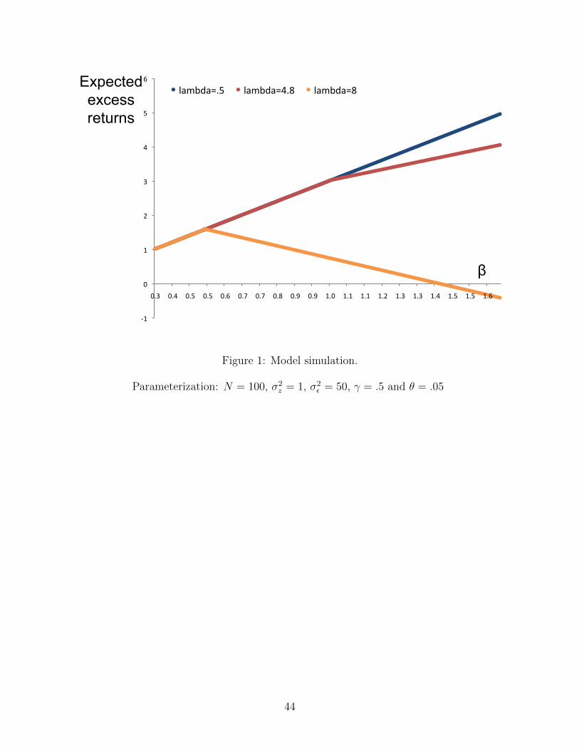
./012/3*(# ./012/3'*,# ./012/3,#

!

Expected

excess

returns

Figure 1: Model simulation.

Parameterization: N = 100, σ2z = 1, σ2

= 50, γ = .5 and θ = .05

44

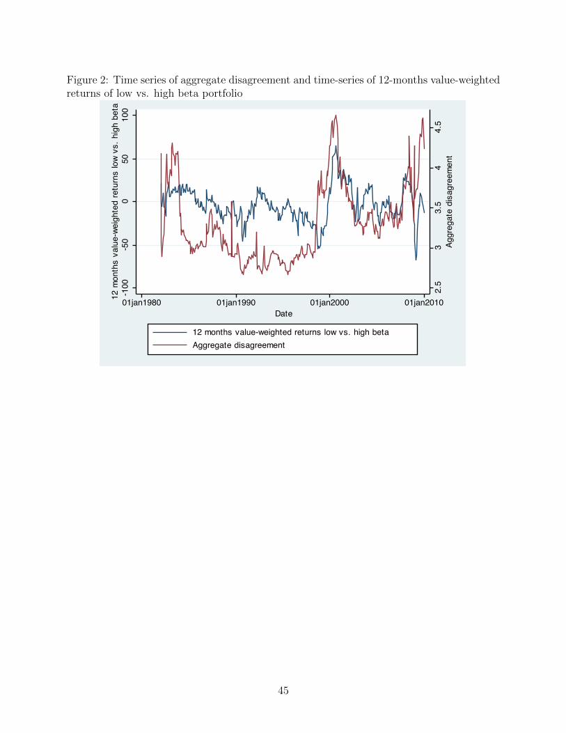
Figure 2: Time series of aggregate disagreement and time-series of 12-months value-weightedreturns of low vs. high beta portfolio

2.5

33

.54

4.5

Ag

gre

ga

te d

isa

gre

em

ent

-100

-50

05

01

00

12 m

onth

s v

alu

e-w

eig

hte

d r

etu

rns

low

vs

. h

igh b

eta

01jan1980 01jan1990 01jan2000 01jan2010

Date

12 months value-weighted returns low vs. high beta

Aggregate disagreement

45

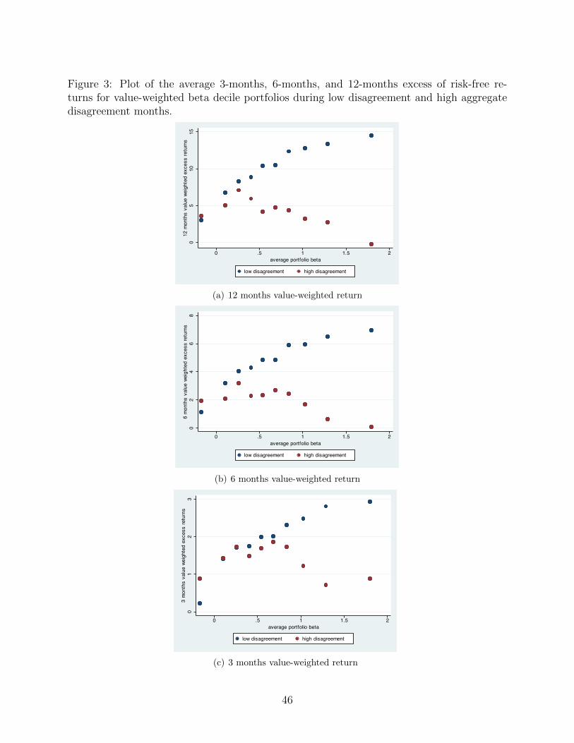
Figure 3: Plot of the average 3-months, 6-months, and 12-months excess of risk-free re-turns for value-weighted beta decile portfolios during low disagreement and high aggregatedisagreement months.

05

10

15

12

mo

nth

s v

alu

e w

eig

hte

d e

xc

es

s r

etu

rns

0 .5 1 1.5 2

average portfolio beta

low disagreement high disagreement

(a) 12 months value-weighted return

02

46

8

6 m

on

ths

va

lue

we

igh

ted

ex

ce

ss

re

turn

s

0 .5 1 1.5 2

average portfolio beta

low disagreement high disagreement

(b) 6 months value-weighted return

01

23

3 m

on

ths

va

lue

we

igh

ted

ex

ce

ss

re

turn

s

0 .5 1 1.5 2

average portfolio beta

low disagreement high disagreement

(c) 3 months value-weighted return

46

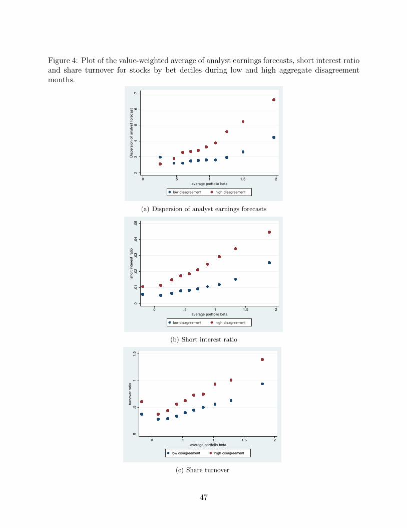
Figure 4: Plot of the value-weighted average of analyst earnings forecasts, short interest ratioand share turnover for stocks by bet deciles during low and high aggregate disagreementmonths.

23

45

67

Dis

pe

rsio

n o

f a

na

lys

t fo

rec

as

t

0 .5 1 1.5 2

average portfolio beta

low disagreement high disagreement

(a) Dispersion of analyst earnings forecasts

0.0

1.0

2.0

3.0

4.0

5

sh

ort

in

tere

st

ratio

0 .5 1 1.5 2

average portfolio beta

low disagreement high disagreement

(b) Short interest ratio

0.5

11

.5

turn

ov

er

ratio

0 .5 1 1.5 2

average portfolio beta

low disagreement high disagreement

(c) Share turnover

47

Figure 5: Aggregate disagreement and Failure of CAPM

-100

-50

050

10

0

2 3 4 5 6

Aggregate disagreement

12 months value-weighted returns low vs. high beta Fitted values

48