speculators and middlemen: the strategy and performance of
TRANSCRIPT

[23:02 27/9/2020 RFS-OP-REVF200046.tex] Page: 5212 5212–5247
Speculators and Middlemen: The Strategyand Performance of Investors in the HousingMarket
Patrick BayerDuke University and NBER
Christopher GeisslerISO New England
Kyle MangumFederal Reserve Bank of Philadelphia
James W. RobertsDuke University and NBER
Using data from the Los Angeles area from 1988 to 2012, we study the behavior andsources of returns of individual investors in the housing market. We document the existenceof two distinct investor types. The first act as middlemen, purchasing substantially belowand reselling above market prices throughout the cycle, improving liquidity and the existingcapital stock in the process. The second act as speculators, who primarily enter during theboom, buying and selling at essentially market prices. Neither type anticipated the housingbust. We document similar behavior by speculators and middlemen in 96 other U.S. metroareas. (JEL D40, D84, R30)
Received July 21, 2017; editorial decision October 26, 2019 by Editor Stijn VanNieuwerburgh. Authors have furnished an Internet Appendix, which is available on theOxford University Press Web site next to the link to the final published paper online.
We thank Ed Glaeser, Matt Kahn, Chris Mayer, Fernando Ferreira, Donghoon Lee, Andy Haughwout, WilbertVan der Klauww, Steve Ross, Amine Ouazad, Todd Sinai, and Joe Gyourko and the seminar participants atHarvard University, University of California at Berkeley and the Haas School of Business, London School ofEconomics, Mannheim, Toulouse, Zurich, University of Georgia, INSEAD, CREST, Northwestern Universityand Kellogg Business School, Duke-ERID Housing Market Dynamics Conference, HULM conference, and theUCLA Housing Market Conference for their useful feedback on the paper. We are grateful for Duke University’sfinancial support. The views expressed in this paper are solely those of the authors and do not necessarily reflectthe views of the Federal Reserve Bank of Philadelphia or the Federal Reserve System. Any errors are our own.Supplementary data can be found on The Review of Financial Studies web site. Send correspondence to PatrickBayer, Duke University, 213 Social Sciences Building, 419 Chapel Drive, Durham, NC 27708-0097; telephone:919-660-1800. E-mail: [email protected].
The Review of Financial Studies 33 (2020) 5212–5247© The Author(s) 2020. Published by Oxford University Press on behalf of The Society for Financial Studies.All rights reserved. For permissions, please e-mail: [email protected]:10.1093/rfs/hhaa042 Advance Access publication April 6, 2020
Dow
nloaded from https://academ
ic.oup.com/rfs/article/33/11/5212/5816604 by D
uke University user on 10 February 2021

[23:02 27/9/2020 RFS-OP-REVF200046.tex] Page: 5213 5212–5247
Speculators and Middlemen
The recent housing boom and bust in the United States affected millions ofhouseholds and hindered the country’s emergence from the Great Recession.1
Housing market investors accounted for a large fraction of transactions duringthe boom and recent evidence suggests they causally fomented the steep runupin prices.2 How did these investors behave and how did they affect the actualfunctioning of the housing market itself? Modern investment theory provides avariety of models that admit a wide range of investor strategies and influenceson a market. However, despite the richness of investor behavior and strategiesin the theory literature, little evidence exists describing how investors actuallybehave in many market settings. How well-informed real investors are, whetherthey behave in a manner consistent with naïve or rational decision-making, andwhether the activity of various types of investors is sufficient to be quantitativelyimportant for equilibrium price dynamics remain key, and open, empiricalquestions.
In this paper we use transaction-level data from the Los Angeles metroarea3 between 1988 and 2012 to characterize the behavior, performance, andstrategies of investors in the housing market. In so doing we marshal three keybroad forms of evidence about the role of investors in this market.
First, we document that a large share of the properties that were purchased inthe Los Angeles market late in the boom were bought by those already holdinganother property in the area, presumably as an investment property. Thesefindings are in line with those of Haughwout et al. (2011), Bhutta (2015), andDeFusco, Nathanson, and Zwick (2017). The sheer magnitude of the activityof novice investors suggests they play a nonnegligible role in the market andsupports at a basic level their use in theory.
Second, we identify different investor strategies in the housing market.For this portion of our analysis, we focus primarily on the behavior of aset of individuals that we observe reselling investment properties after shortholding periods, using the colloquial name “flippers.” Relative to most financialproducts, tracking investment behavior in a durable good like housing iscomplicated by the fact that owners may invest in the good before reselling.In that event, a portion of any price appreciation is likely due to suchimprovements, not just any particular ability of the investor to buy cheap, orsell dear. To address the challenge this creates for understanding the sourcesof returns, we introduce a novel research design using properties that sellrepeatedly during the study period to decompose the observed price growthduring the flipper’s holding period into four components: (1) the discountrelative to market price at the time of purchase, (2) the premium relative to
1 See, for example, Mayer, Pence, and Sherlund (2009), Mian and Sufi (2014), and Rognlie, Shleifer, and Simsek(2018).
2 See, for example, Chinco and Mayer (2016) and Gao, Sockin, and Xiong (2017).
3 Although Los Angeles is the primary focus of the paper, we provide evidence from nearly 100 other metro areasthat the patterns we document in Los Angeles generalize across a wide range of other U.S. cities.
5213
Dow
nloaded from https://academ
ic.oup.com/rfs/article/33/11/5212/5816604 by D
uke University user on 10 February 2021

[23:02 27/9/2020 RFS-OP-REVF200046.tex] Page: 5214 5212–5247
The Review of Financial Studies / v 33 n 11 2020
market at the time of sale, (3) the market return during the holding period,and (4) physical improvements made to the property by flippers. Our researchdesign distinguishes any costly improvements that a flipper may have made(which are not directly observed in the data) by measuring the extent to whichany above-market appreciation that a flipper earns at sale persists through asubsequent sale of the same property.
This analysis illuminates two distinct types of investors in the housingmarket. The first type acts as an intermediary or middleman who purchasesproperties at prices well-below market value and resells them quickly at orabove market prices. The steep discount that they receive by locating “gooddeals” and buying from “motivated” sellers accounts for the majority of theirreturns. Market timing, on the other hand, is not an important source of theirreturns; in fact, they operate more intensely during periods when prices arestagnant or declining and systematically target submarkets that are appreciatingmore slowly than the rest of the metro area.
Their behavior contrasts sharply with that of the novice investor or speculatorthat entered the market in droves during the boom. Relative to market prices,these investors do not buy at much of a discount or sell at much of a premium,suggesting that most are not inordinately skilled real estate professionals.Instead these novice investors earn most of their return through the marketappreciation over the period that they hold the property. Speculators operateprimarily during boom times and purchase homes in submarkets of the LosAngeles area that experience both an above average rate of appreciation inthe short term (1–2 years) and a sharp decline in the intermediate term (3–5years). After controlling for transaction costs, we find that realized returns formiddlemen are nearly twice that of speculators.4
To further support and provide external validity for our findings about theLos Angeles housing market, we extend our framework to 96 other U.S. metroareas.5 We show that speculators and middlemen operate in other markets aswell. Our results suggest that the investor strategies and behaviors we documentin Los Angeles are representative of broader patterns in the housing market.
Third, having established distinct investor types that follow differentstrategies, we ask how these investor types interact with the broader housingmarket. Here, we focus on three channels. First, we examine whether the noviceinvestors that purchased homes late in the boom were able to anticipate themarket peak, or instead seem to exhibit trend chasing behavior. Remarkably,they continued to purchase homes at near-record rates right up to the peak,and there is no change in the rate at which they sold their existing holdings,despite a clear financial incentive to do so. Second, we show that middlemen
4 As we note elsewhere, because we cannot observe rental income or any particular investor’s specific tax rate, weare somewhat limited in our ability to accurately measure the precise levels of returns.
5 The selection of the other metro areas for analysis is mainly determined by data availability. See the discussionin Section 4.
5214
Dow
nloaded from https://academ
ic.oup.com/rfs/article/33/11/5212/5816604 by D
uke University user on 10 February 2021

[23:02 27/9/2020 RFS-OP-REVF200046.tex] Page: 5215 5212–5247
Speculators and Middlemen
improve market liquidity as they are more likely than a typical homeowner tobuy a property not currently in use. In contrast, speculators are no more likelythan a typical homeowner to buy such properties. Third, we show more directevidence that middlemen improve the quality of the housing stock by investingin the properties they own, as measured by the frequency with which they areissued permits for construction and home improvements. Speculators, on theother hand, take out permits no more frequently than does a normal homeowner.
Taken as a whole, the various forms of evidence that we present providesa comprehensive picture of the activity of investors in the housing boomthat is consistent with the behavior captured in many theoretical models offinancial markets. We find no indication that the speculators that poured into themarket late in the boom had access to superior information, which is consistentwith the notion that many of these investors had very limited experience andmay have simply been swept up in the exuberance of the boom. This is ofcourse also consistent with famous accounts of speculative activity by CharlesMackay6 and Kindelberger (1978), who in his “anatomy of a typical crisis”notes that bubbles are frequently characterized by “More and more firms andhouseholds that previously had been aloof from these speculative ventures”beginning to participate in the market. Some of these speculators, to be sure,earned substantial returns via successful market timing. But the evidencethat speculators were not particularly more well-informed casts doubt on thenotion that they improved efficiency by transmitting any valuable informationto the market. Middlemen, on the other hand, appear to operate throughouthousing cycles and likely improve the market’s liquidity and capital stock. Moregenerally, that these flippers were party to such a large number of transactionsduring the final few years of the housing boom not only justifies their useas a theoretical device but also suggests that their activity may be of first-order importance from a policy perspective, a topic we turn to in the paper’sconclusion.
1. Related Literature
Our paper is connected to and contributes to a number of literatures. Housingmarkets are a classic example of a thin market for high-valued durable goodsin which sellers with heterogenous holding costs (because of, say, differingrelocation or borrowing cost needs)7 and buyers with heterogeneous values forany given home (because of, say, its location or horizontally differentiatedcharacteristics) must engage in costly search in order to transact. Flippers
6 In his well-known description of the boom and bust in the 1637 Dutch tulip market Mackay commented that atits peak, “Nobles, citizens, farmers, mechanics, seamen, footmen, maid-servants, even chimney-sweeps and oldclotheswomen, dabbled in tulips” (see Mackay (1841), p. 94).
7 Springer (1996) finds that distressed sellers deal more quickly and sell for less than other sellers. Glower, Haurin,and Hendershott (1998) find that when a seller takes a new job, she sells faster than average, indicating a higherholding cost.
5215
Dow
nloaded from https://academ
ic.oup.com/rfs/article/33/11/5212/5816604 by D
uke University user on 10 February 2021

[23:02 27/9/2020 RFS-OP-REVF200046.tex] Page: 5216 5212–5247
The Review of Financial Studies / v 33 n 11 2020
who purchase a property with plans to put the house back on the market areacclimated to such a market. We provide evidence that flippers participated ina sizable share of housing transactions during the recent boom and bust. Inthis way, our results complement those in Haughwout et al. (2011) and Bhutta(2015). Though the absolute magnitude of the overall housing ownership byinvestors may not be large, as Piazzesi and Schneider (2009) argue, even asmall number of optimistic investors that participate in housing transactionscan meaningfully affect housing prices. Indeed, recent work has argued thatreal estate investors causally increased housing prices during the boom (Chincoand Mayer 2016; Gao, Sockin, and Xiong 2017).
How did these investors behave? Modern finance theory admits a wide rangeof possible answers to this question and our paper explores this topic in detail.In general, the economic function of flippers that buy properties from especiallymotivated sellers, hold them for a short period, and then sell them to a buyer thatplaces a sufficiently high value on the property is that of a middleman.8 Beyondthe need to set prices and clear markets or guarantee quality, a crucial role formiddlemen is to provide liquidity and immediacy to transactions (see, e.g.,Demsetz 1968; Garman 1976; Amihud and Mendelson 1986; Copeland andGalai 1983; Glosten and Milgrom 1985; Kyle 1985). In durable goods marketsthey can also invest in the asset during the holding period. For middlemen,opportunities to buy may occur under any market conditions, provided theyare able to identify especially motivated sellers (those with higher holdingcosts than their own), and we provide evidence that many flippers operate asmiddlemen throughout the housing cycle and perform these central functions.
Flippers can also act as speculators in the housing market. If flippers haveaccess to better information than the broad set of agents participating ina market, which is plausible given the decentralized nature of the housingmarket and the infrequency with which a typical household moves, they maybe able to exploit arbitrage opportunities. In the classic theory of efficientmarkets, speculators, acting on the basis of their superior information, serveto align prices more closely with market fundamentals, generally improvingthe efficiency of the market (Fama 1965). But modern finance theory admits awider range of strategies for speculators and a more ambiguous understandingof their impact on welfare and efficiency.9,10 In the presence of noise tradersthat behave according to heuristics like chasing trends, prices can temporarilydeviate from fundamentals and the rational speculator may not wish to simplytake a short position. In fact, it can be optimal to pursue a much wider rangeof strategies. If, for example, noise traders engage in positive feedback trading,that is, have a tendency to extrapolate or to chase the trend, it can be optimal
8 Spulber (1996) provides a nice discussion of the roles of middlemen.
9 See Shleifer and Summers (1990), Barberis and Thaler (2003), and Shiller (2003) for summaries of this literature.
10 Differing levels of risk aversion, which may vary over time, may also lead some people to buy an asset. We thankan anonymous referee for encouraging us to point this out.
5216
Dow
nloaded from https://academ
ic.oup.com/rfs/article/33/11/5212/5816604 by D
uke University user on 10 February 2021

[23:02 27/9/2020 RFS-OP-REVF200046.tex] Page: 5217 5212–5247
Speculators and Middlemen
for rational speculators to jump on the bandwagon (DeLong et al. 1990). In thiscase, rational speculators take advantage of the noise traders by strategicallyselling before the noise traders realize the bubble is about to burst. In this way,the welfare consequences of the existence of speculators need not be positive. Ingeneral, speculators will require expected market appreciation to be sufficientlyhigh to justify their purchases and, therefore, will be active in only those timesand places where conditions are right. Here, we show dynamic patterns of asubset of investors that align with these predictions.11
Finally, our paper is connected to a rich strand of research investigatingspecific episodes throughout history to understand the actions of investors ina variety of financial markets. For example, we show that investors were notable to anticipate the housing market’s peak. Our findings complement thoseof Cheng, Raina, and Xiong (2014), who demonstrate that agents workingin securitization finance, and thus who were likely to be as informed aboutthe housing market’s fundamentals as anyone, and which is a market that hasbeen linked to the boom and bust in housing, were not able to predict themarket’s crash. In contrast to these results, Temin and Voth (2004) study asophisticated investor who successfully profited from “riding” the South Seabubble and Brunnermeier and Nagel (2004) find that hedge funds were ablereduce their exposure to tech stocks before the dot-com bubble burst. Otherstudies of bubble-like episodes include Garber (1989), who studies the Dutchtulip bubble, Greenwood and Nagel (2009) and Griffin et al. (2011), who, alongwith others, study investor behavior during the dot-com bubble, and Rajan andRamcharan (2015), who study the rise and fall of U.S. farmland prices in the1920s. In general we view the investigation of investor behavior in the housingmarket as particularly important for a variety of reasons, not the least of whichis that housing is the asset which typically comprises the greatest share of ahousehold’s wealth.12 Other recent work exploring the quantitative importanceof housing market speculators includes Mian and Sufi (2018).
2. Data
The primary data set that we have assembled for our analysis is based ona large database of residential housing transactions compiled by DataquickInformation Services, a national real estate data company. Dataquick acquiresdata from public sources like local tax assessor offices, and they have providedus with the complete census of housing transactions in the five largest countiesin the Los Angeles metropolitan area (Los Angeles, Orange, Riverside, San
11 In a recent paper, DeFusco, Nathanson, and Zwick (2017) also find evidence that inexperienced speculatorsdisproportionately enter the market in boom times, and the authors also provide a theoretical explanation for whythis is the case.
12 Bostic, Gabriel, and Painter (2009) document that, by 2004, housing had grown to compose more than 50% ofa typical household’s wealth.
5217
Dow
nloaded from https://academ
ic.oup.com/rfs/article/33/11/5212/5816604 by D
uke University user on 10 February 2021

[23:02 27/9/2020 RFS-OP-REVF200046.tex] Page: 5218 5212–5247
The Review of Financial Studies / v 33 n 11 2020
Bernardino, and Ventura), between 1988 and the third quarter of 2012. Foreach transaction, the data contain the names of the buyer and seller, thetransaction price and date, the address, and numerous characteristics including,for example, square footage, year built, number of bathrooms and bedrooms,lot size, and whether the house has a pool. While we are able to observe thedate, price, and names of the buyer and seller for every transaction in the data,a drawback of the data is that Dataquick only maintains a current assessorfile and overwrites historical information on house characteristics. This meanswe observe housing characteristics as they were in 2012, and consequentlywe cannot see how they may have evolved over time. The assessor data does,however, include a field with the year of permitted improvements to the property,if any, but it does not detail the change in property characteristics. This datalimitation will partially motivate our research design to control for unobservedinvestment in houses that is explained below, although a research design toaddress the possibility of unobserved improvements to properties would benecessary even if Dataquick kept track of housing attributes on a continuousbasis, as many home improvements (e.g., a renovated kitchen or bathroom)would not generally affect the more basic attributes of the home (e.g., lot size,square footage, room partitions) collected by the tax assessor.
From the original census of transactions, we drop observations if a propertywas subdivided or split into several smaller properties and resold, the transactionwas flagged as not being arm’s-length, the price of the house was $1 or less,13 thehouse sold more than once in a single day, the property was especially unusualin that the price or square footage was in the top or bottom 1% of the sample, orthere is a potential inconsistency in the data, such as the transaction year beingearlier than the year the house was built (which may be land transactions).By observing the full transaction history for each property, we are able to seewhether the buyer resold the home (versus holding to the end of the sample ortransferring the property in a non-arm’s-length transaction or foreclosure) and,if so, how long it was held in the interim.
Table 11 in Appendix 1 provides summary statistics for our primary dataset based on a full sample of over 4.75 million transactions between 1988 and2012. Figure 1 shows the dynamics of prices and transaction volume for the LosAngeles metropolitan area over the study period. The price index is computedwith our data using a standard repeat sales method that we describe in Section2.4. Following a rapid increase in prices in the late 1980s, the early 1990s werea “cold” market period for Los Angeles, with prices declining by roughly 30%between 1992 and 1997 and transaction volume averaging only a little morethan 30,000 houses per quarter during this period. Starting in the late 1990sand continuing until early 2006, the Los Angeles housing market experienced amajor boom, with house prices more than tripling and transaction volume nearly
13 Such a low price indicates that the seller did not put the house on the open market and instead transferredownership in a non-arm’s-length transaction.
5218
Dow
nloaded from https://academ
ic.oup.com/rfs/article/33/11/5212/5816604 by D
uke University user on 10 February 2021

[23:02 27/9/2020 RFS-OP-REVF200046.tex] Page: 5219 5212–5247
Speculators and Middlemen
Figure 1Price and quarterly transaction volumeThe figure reports quarterly transaction volume and a log price index for arm’s-length sales in the greater LosAngeles metropolitan area. The price index is derived from a repeat sale regression described in Section 2.4,with normalization to one in 1988:Q1.
doubling. Just 2 years later almost all the appreciation in house prices from theprevious decade had evaporated and transaction volume had fallen to recordlow levels (less than 20,000 houses per quarter). In the analysis below, we willreference the three key market periods evident in Figure 1: the “cold” marketperiod (1992–1998), the “hot” or boom market period (1999–2006Q2), andthe “post-peak” period (2006Q3–2009). While we generally will exclude theperiods 1988–1991 and 2010–2012 from our analyses of investment purchases,it is useful to have both pre- and post-study period data because measurement ofmany of our definitions and outcomes rely on the entire history of the buyer andseller and the properties themselves. Our main analyses, in particular, employa repeat sales framework, so it is useful to observe more transactions of eachproperty.
2.1 FlippersA basic measurement challenge for anyone wishing to study the behavior ofinvestors in the housing market in these data is identifying such agents in thefirst place.14 Figure 2 reports the time series for four measures of investorbehavior in the Los Angeles market between 1992 and 2012 derived from ourtransaction data set. The first of these, labeled “Second Homes,” is constructedin the spirit of Haughwout et al. (2011) by identifying individuals that own two
14 Appendix 2 discusses other approaches in the literature for identifying housing market investors.
5219
Dow
nloaded from https://academ
ic.oup.com/rfs/article/33/11/5212/5816604 by D
uke University user on 10 February 2021

[23:02 27/9/2020 RFS-OP-REVF200046.tex] Page: 5220 5212–5247
The Review of Financial Studies / v 33 n 11 2020
Figure 2Quarterly residential real estate investment activityThe figure plots the quarterly share of investment activity under multiple (nonexclusive) definitions of real estateinvestors using transactions data for the greater Los Angeles metropolitan area. See the main text for more details.
homes at the same time. In particular, we categorize a property as a secondhome if the buyer’s name matches that of an individual that we also observeto be simultaneously holding another property in our data set.15 The use ofbuyer names is a potential source of error that we address in detail below.An advantage of our procedure is that it relies on only the deeds history fileitself, and not external sources like property tax address or credit histories. Afundamental problem with this definition, of course, is that for an individual tobe observed as a homeowner at all, they need to have purchased a home since thebeginning of our data in 1988. Thus, our measure of “Second Homes” is likelyto understate the amount of actual second home purchases, especially near thebeginning of the sample period (note the figure’s series begins in 1992). For thisreason, one should not overinterpret the trend in the measure. However, evensubject to these various limitations, our measure of second home purchasesclosely tracks that of Haughwout et al. (2011), rising to a peak of nearly 24%of the market in 2006.
Many housing market investors ought not to be considered “flippers,” becausemotivations aside from speculation, arbitrage, or property improvement candrive investment in housing. One concrete example is the aim to rent theproperty. We are particularly interested in individuals buying with the intentionof reselling the property after a relatively short holding period. To identifyflippers, therefore, we look for evidence that an individual is generally engaged
15 This count ignores properties that overlap for 6 months or less to allow for a typical search time during householdmoves.
5220
Dow
nloaded from https://academ
ic.oup.com/rfs/article/33/11/5212/5816604 by D
uke University user on 10 February 2021

[23:02 27/9/2020 RFS-OP-REVF200046.tex] Page: 5221 5212–5247
Speculators and Middlemen
in such a strategy. In this spirit, we generate a second time series shown inFigure 2, “Purchases Resold Within Two Years”, which simply reports thefraction of all homes (regardless of the buyer) purchased in a given quarter thatare subsequently resold within 2 years time. Nearly 15% of all homes purchasednear the peak of the boom in 2003–2005 were resold within 2 years, a rate thatis more than triple the corresponding rate for the cold market of 1992–1994or after the 2006 price peak, periods when home prices were declining. Whilecertainly a portion of the buyers that resell homes within 2 years of purchase areowner-occupants rather than investors, this time series provides an initial proxyfor flipper-like behavior in the market throughout the cycle and demonstratesthat it is economically significant.
For much of our analysis, we focus not on flipped homes per se, but on a setof individuals and firms that we identify as flippers. We designate a buyer to be aflipper from one of two (not mutually exclusive) conditions from the investmentproxy series just presented. One is an overlapping property tenure definition,that is, the “second home” method where the buyer is observed to already holdanother property in the Los Angeles market, and the additional property is soldwithin Y years. For most of our analysis we use Y =2, but we will examine howoutcomes vary with respect to hold time. Another definition is to observe thebuyer engaged in the buying and selling at least X different properties whileholding them for less than Y years, as in the “Purchases Resold Within Y ”definition. For this definition, we usually set X=2 and again Y =2, though amajor focus of our analysis is how flipper behavior, strategy, and returns varywith X.16 The difference from the first definition is that the second does notrequire contemporaneous overlap in property holdings, but the individual mustconduct a “flip” multiple times.17
Limiting our definition of flippers in these ways provides a conservativemeasure of flipper activity, as we miss any individuals who engage in thisactivity only once during the sample period without an overlap with an existingproperty, or those who tend to hold properties for slightly longer periods oftime, or any out-of-town investors who purchase only one investment. We dothese to make sure that we avoid (as much as possible) counting normal owner-occupants as flippers. To the extent that we categorize some investors as normalowner-occupants, we would expect such contamination to cause attenuation inour measures of outcomes. Each of these measures relies on the name matchesavailable in the transactions register and we detail this procedure in Appendix 3and perform a number of robustness checks to possible complications associatedwith the procedure.
16 The latter condition would catch investors whose primary residence is “out of town” if they conduct sufficientlymany flips within Los Angeles. For more on out-of-town investors, see Favilukis and Van Nieuwerburgh (2018)or Chinco and Mayer (2016).
17 Table 12 in Appendix 1 provides the purchase frequency distribution for individuals we have classified as normalowner-occupants, investors (not flippers), flippers, and institutional buyers with nonpersonal names (such asbusinesses, various government entities, and places of worship).
5221
Dow
nloaded from https://academ
ic.oup.com/rfs/article/33/11/5212/5816604 by D
uke University user on 10 February 2021

[23:02 27/9/2020 RFS-OP-REVF200046.tex] Page: 5222 5212–5247
The Review of Financial Studies / v 33 n 11 2020
Figure 3Flipper purchases over time by flipper typeThe figure plots the quarterly share of flipper purchases by flipper volume type. Low volume: 1-2 flips in availabledata; medium-low volume: 3-5 flips; medium-high Volume: 6-9 flips; high volume: 10 or more flips.
Figure 2 shows the flipper data series. “Purchases by Flippers” reports thefraction of housing transactions in each quarter that were made by individualsthat we define as flippers. Note that this measure includes all homes purchasedby flippers regardless of how quickly these homes are resold. This time seriesgenerally tracks housing market conditions, peaking at nearly 10% of allpurchases from 2004 to 2006, a rate 3 times higher than the rate of flipperactivity in the early 1990s. The last series, “Flips,” represents properties heldless than 2 years and purchased by individuals designated as flippers. As theintersection of the last two series, the pattern over time shows similar cyclicalbehavior to all purchases by flippers, though the peak comes sooner in about2005. It is plausible that some 2006 purchases were intended to be flips, onlyto see prices fall precipitously in the coming 1 to 2 years and then not resold.18
Overall, the four broad metrics of aggregate investor or flipper activity shownin Figure 2 depict a consistent pattern of procyclical behavior, with the shareof purchases by these agents reaching a maximum at the peak of the housingboom, at levels that are roughly 3 times the level of activity observed during themarket trough in the early 1990s. Below, we will distinguish between investortypes whose strategies and participation over the housing cycle differ from oneanother.
18 We examine sale propensity over the cycle in Section 5.2.
5222
Dow
nloaded from https://academ
ic.oup.com/rfs/article/33/11/5212/5816604 by D
uke University user on 10 February 2021

[23:02 27/9/2020 RFS-OP-REVF200046.tex] Page: 5223 5212–5247
Speculators and Middlemen
2.2 Purchase activity by flipper typeIn the analysis that follows, we document considerable heterogeneity in flipperbehavior, strategy, and outcomes that is strongly associated with the individualflipper’s volume of investments. Figure 3 shows the share of transactions ina given quarter by flippers in four volume categories. We define low-volumeflippers as those flipping one or two properties, medium-low as three to five,medium-high as six to nine, and high volume as 10 or more. For the purposesof this definition, we count a purchase as a flipped home if it was resold within2 years, and we categorize flippers on the basis of their activity over the fulldata period. The reported data series in Figure 3 includes all purchases (flipsand others), and their sum produces the total count of flipper purchases shownin Figure 2.19
Figure 3 clearly illustrates that the dynamics of flipper activity depends onthe individual’s total observed volume. The purchase activity by higher-volumeflippers is relatively constant over the study period, actually peaking in thecolder market period of the mid-1990s. This pattern of activity is consistentwith a view that these flippers tend to operate as middlemen, looking foropportunities to buy from motivated sellers with higher holding costs thantheir own, opportunities that are just as (or perhaps more) likely to arise in coldversus hot market conditions.
In contrast, the purchase activity by lower-volume flippers, especially thelowest category, is highly procyclical, rising from a very small percentageof the overall market in the early- to mid-1990s to almost 8% of the marketin 2004–2006. This pattern of activity is consistent with the view that manynovice investors were drawn into the market during the boom period. Whilethis measure of activity is not enough to establish the motives of these flippers,the timing of their purchases is certainly consistent with a view that they areseeking to make a quick speculative gain on the basis of market appreciation.
It is worth noting that our categorization of flippers is not perfect. Inparticular, our volume measure is based on activity over the full study period.Thus, many of the flippers that we categorize as low volume may, in fact,ultimately become more experienced if they continue to flip homes after ourstudy period ends, a concern mitigated by using data after the market peak.Moreover, survival in the flipping business is likely to be nonrandom, with moreprofitable flippers being more likely to survive long enough in the business toreach the higher-volume categories. In our analysis below, we will explicitlyaddress these and other issues that arise due to our definition of flipper type.
A final, important aspect of flipper purchase activity to describe atthe outset of our analysis is the heterogeneity in the attributes of homespurchased by flippers of each type. To this end, Table 13 in Appendix 1summarizes some basic characteristics of the homes purchased by flippers
19 Series for flips-only show similar patterns.
5223
Dow
nloaded from https://academ
ic.oup.com/rfs/article/33/11/5212/5816604 by D
uke University user on 10 February 2021

[23:02 27/9/2020 RFS-OP-REVF200046.tex] Page: 5224 5212–5247
The Review of Financial Studies / v 33 n 11 2020
of each type. As the table makes clear, flippers, especially high-volumeflippers, generally purchase properties that are older and smaller than theremainder of homes that sell at least twice during our study period. Thesedifferences remain in the lower panel, which uses a regression with flippertype dummies and controls for ZIP-code-level fixed effects. Thus, flippersare buying smaller and older properties than others in the properties’surrounding neighborhoods. The research design that we present below forestimating the sources of flipper returns is motivated in large part by thepossibility that flippers may systematically purchase older homes or “fixeruppers” that can benefit from substantial renovations or improvements beforebeing resold. We also take the additional steps described below to ensurethat we compare the sources of returns for flippers across comparablehouses.
2.3 Flipper holding timesBefore turning to our analysis of the sources of flipper returns, we present afinal descriptive characterization of the heterogeneous behavior of flippers ofeach type. Table 1 reports the fraction of homes sold by the investors we haveclassified as flippers of each type within 1–4 years of the purchase. The tablereveals significant heterogeneity in holding periods by flipper type. Higher-volume flippers, in particular those in the highest volume category, are muchmore likely to resell homes after very short holding periods, selling close to 80%of all of the homes they purchase within the first year and more than 90% within4 years.20 This suggests that these flippers purchase properties with the intentto put them immediately back on the market and is consistent with the notionthat they serve the economic function of middlemen, seeking to buy cheaplyfrom motivated sellers and resell quickly. By contrast, flippers in the lowestvolume category sell only 22% of their purchases within a year of purchase,about half within 2 years, and only 62% by the 4-year mark.21 The overallpattern of behavior is consistent with a strategy of buying properties with theintention of capturing market appreciation, a strategy which, of course, requiresa reasonable holding period.
2.4 Measuring the sources of flipper returns: Research designHaving documented the pattern of purchase activity by flippers, we turn nextto an analysis of the sources of their returns. We will not be able to calculatethe actual profit that a flipper earns on a particular investment because we donot observe several components affecting an individual investment holding,including whether the property is rented to a tenant during a holding period,
20 Table 14 in Appendix 1 shows an expanded version of the table with subpanels devoted to hot and cold periods.This behavior is slightly more pronounced in the cold market period than the hot market.
21 Low-volume types not only have fewer properties held less than 4 years (which is somewhat mechanical, by ourdefinitions), but fewer held for 1 year or less, though the flip definition extends to 2 years holding time.
5224
Dow
nloaded from https://academ
ic.oup.com/rfs/article/33/11/5212/5816604 by D
uke University user on 10 February 2021

[23:02 27/9/2020 RFS-OP-REVF200046.tex] Page: 5225 5212–5247
Speculators and Middlemen
Table 1Property holding times by flipper type
Flipper type Own-occ. Low Med-low Med-high High(no. of flips) 0 1-2 3-5 5-9 10+
Combined periods: 1992-2009
Purchases 1,762,943 111,714 31,253 7,522 8,403Frac. sold within:
1 yr 0.036 0.224 0.398 0.614 0.7862 yrs 0.098 0.452 0.588 0.748 0.8753 yrs 0.189 0.529 0.654 0.800 0.9064 yrs 0.265 0.587 0.698 0.827 0.919
The table reports the fraction of the homes purchased by flippers of different types sold with 1, 2, 3, and 4 years,respectively, in the greater Los Angeles area.
the particular transaction costs that a flipper might pay while buying and sellinga house, or the borrowing costs that a flipper faces when procuring a mortgagein order to purchase a property.
Instead, we will focus only on the components of the returns that areassociated directly with the purchase, holding, and sale of the property, and howthese might correspond to the roles of speculator or middleman. In particular,we seek to identify (1) the discount that flippers receive (relative to the expectedsales price in the market in the corresponding period at the time of purchase),(2) the market return that they earn over the period that they hold the property,and (3) the premium that they receive at the time of sale (again relative to theexpected sales price in the market at the time). By measuring these sources offlipper returns, we seek to categorize flippers on the basis of their motivationand strategy to identify whether they appear to be operating as middlemen orspeculators.
An important complicating factor is that flippers may systematically makephysical improvements to the properties that they purchase, improvementswhich are unobserved in our data set for the reasons mentioned in Section2. The concern is that a naive analysis of the sources of flipper returns frombuying, holding, and selling a property might wind up counting money thatflippers invested in improving a property as part of their return. This would beespecially worrisome for our purposes if flippers of different types modifiedthe properties in different ways.
To address this problem, we develop a research design that aims to uncoverthe sources of flipper returns from buying, holding, and selling a property inthe (potential) presence of unobserved investment. The design is a modifiedversion of the classic repeat sales method (Case and Shiller 1987):
log(pit )=αt +γi +β1kbkit +β2kskit +β3kakit +εit . (1)
In Equation (1), αt are time period (e.g., quarter) fixed effects and γi are house-level fixed effects. Exponentiating the estimated time fixed effects gives theprice index for each quarter, which can be normalized to 1 in any quarter. Thefirst departure from the standard repeat sales method comes from including bkit ,
5225
Dow
nloaded from https://academ
ic.oup.com/rfs/article/33/11/5212/5816604 by D
uke University user on 10 February 2021

[23:02 27/9/2020 RFS-OP-REVF200046.tex] Page: 5226 5212–5247
The Review of Financial Studies / v 33 n 11 2020
a dummy for if the buyer is a flipper of type k = {low,medium-low,medium-high,high}, and skit , a dummy for if a flipper of type k is the seller. Theseestimated coefficients related to flipper activity will provide estimates of thediscount that flippers receive when buying (should β̂1k <0) and the premiumthey command when selling (should β̂2k >0), provided that house quality isconstant over time. If, however, flippers purchase houses and then invest heavilyto improve them before putting them back on the market, these parameterestimates will be biased. In particular, we would expect β1k to be negativebecause the true house quality in this period would be less than the estimatedquality. Similarly, β2k would likely be positive because the true quality inthis period would be greater than the quality estimated. The researcher may,therefore, infer that flippers are buying at a discount and selling at a premiumwhen they are simply investing more than the average homeowner. This iswhy we further depart from the standard repeat sales method by including akit ,which is equal to one if, in any previous period, we see a flipper of type k
purchase house i, and thus allows us to control for any improvements madeby the flipper that extend beyond average homeowner investment because β3k
captures the change in house quality between when the flipper purchased andsold the home.22
In the standard repeat sales framework, a house only helps to identify thetime series of market appreciation when it sells at least twice; otherwise itcan only identify its corresponding house fixed effect. However, to identifythe coefficients corresponding to the sources of flipper returns and investment,β1k,β2k and β3k in Equation (1), homes must sell at least 4 times, with at leastone nonflipper to nonflipper transaction before and after a flipper buys and sellsthe house in order to identify its own fixed effect and the flipper coefficients. Weterm this “ABCD” structure: at A both transacting parties are nonflippers; at Bthe house is sold to a flipper by the nonflipper; at C the flipper sells the house to anonflipper; and at D it is sold to a nonflipper by the nonflipper. The observationbefore the flipper buys is used to identify the original house quality and theobservation after the flipper sells is used to identify the new house quality, whileconcurrent nonflipper to nonflipper transactions on other properties identify themarket trend. Appendix 4 further illustrates the identification argument.
Note that because our estimates of the sources of flipper returns will be basedon properties that sell between normal owner occupants and fit this ABCDstructure, then by construction, the period of time that the previous owner helda property before selling to a flipper is limited (as the sale at point A must bewithin the sample period). This excludes houses that may have been neglectedover a long period of time by an owner from contributing to our estimates of the
22 Using information in the tax assessor data, we also include controls for whether the transaction is observed beforeor after a permitted improvement to the property. However, because there may be heterogeneity in the value ofinvestment not captured by a permit-issuance dummy and some investments do not require permits, we includethe akit controls.
5226
Dow
nloaded from https://academ
ic.oup.com/rfs/article/33/11/5212/5816604 by D
uke University user on 10 February 2021

[23:02 27/9/2020 RFS-OP-REVF200046.tex] Page: 5227 5212–5247
Speculators and Middlemen
sources of flipper returns.23 While flippers, especially those seeking to makesignificant physical improvements, may target such homes, they generally willnot be the ones that identify the sources of returns given our research design.
In the analysis that follows, we report results for two slight adjustmentsto the specification shown in Equation (1). First, we include a series ofdummy variables for how many times we have seen a given propertypreviously transacted in the study period. In general, sellers make some homeimprovements at the time of a sale so that a house will show well. Thus, weinclude these additional sales number dummy variables to avoid systematicallyoverstating the performance of homes that meet the ABCD structure simplybecause they sell at least 4 times during the study period. Second, as shown inTable 13, flippers (especially experienced flippers) tend to purchase homes thatare slightly older and smaller than the average homes that are sold in the market.Therefore, to ensure that we are comparing apples to apples, we report resultsfor a second specification of Equation (1) that interacts the three key flippervariables with demeaned measures of housing attributes, reporting the flippercoefficients at the mean attributes of the homes sold in the study period. Thisensures that all comparisons of sources of returns are done for the same type ofproperty, even though flippers of different types may purchase properties thatare somewhat heterogeneous.
3. Sources of Flipper Returns: Baseline Results
3.1 Average flipper returnsWe now provide estimates of the sources of flippers’ returns using the aboveresearch design. Table 2 presents our initial results for all flipper types. Thetable abbreviates the main coefficients of interest (Appendix Table 15 reportsexpanded results with control variables). The analysis includes all the data from1988 to 2012 to account for as many repeat sales as possible, but flipper activityis based on purchases made in the years between 1992 and 2009. We exclude theends of the sample from flip designation because we need some buyer historyto designate investments and then must follow the properties for at least 2 (ormore) years to identify it as a flip.
Column 1 presents estimates from a simplified version of specification (1)which omits akit . The controls for improvements made by the flipper in thesimple specification are the permit issuance dummy (which is significant andpositive), and sale number dummies. The coefficient estimates indicate that apurchase designated as a flip implies an 11% discount, and the sale of the flipcomes at a 7% premium relative to the expected market value of the property
23 In fact, a comparison of the housing attributes of homes that meet the ABCD structure reveals less heterogeneityin the properties that flippers purchase versus the average homes that sell in the market as a whole. For example,the average age of the homes purchased by high-volume flippers decreases from 44 to 41 years when the sampleis limited to just homes that meet the ABCD structure.
5227
Dow
nloaded from https://academ
ic.oup.com/rfs/article/33/11/5212/5816604 by D
uke University user on 10 February 2021

[23:02 27/9/2020 RFS-OP-REVF200046.tex] Page: 5228 5212–5247
The Review of Financial Studies / v 33 n 11 2020
Tabl
e2
Aug
men
ted
repe
atsa
les
regr
essi
onre
sult
s:A
llfli
pper
type
sco
mbi
ned
12
34
56
Col
dH
otPo
stpe
akFl
ipqt
rof
purc
h.19
92-’
0919
92-’
0919
92-’
0919
92-’
0919
92-’
0919
92-’
9819
99-’
06Q
220
06Q
3-’0
9
Flip
purc
hase
(β1
)−0
.115
2−0
.120
0−0
.102
8−0
.111
8−0
.093
3−0
.206
3−0
.071
4−0
.185
9(0
.001
3)(0
.001
4)(0
.001
3)(0
.001
5)(0
.002
1)(0
.003
6)(0
.001
7)(0
.005
4)Fl
ipsa
le(β
2)
0.07
620.
0594
0.01
730.
0684
0.07
840.
0509
0.05
400.
0447
(0.0
011)
(0.0
012)
(0.0
011)
(0.0
014)
(0.0
019)
(0.0
026)
(0.0
016)
(0.0
070)
Flip
inve
stm
ent(
β3
)0.
0207
0.01
870.
0333
0.00
210.
0700
(0.0
016)
(0.0
017)
(0.0
032)
(0.0
018)
(0.0
058)
Inte
ract
prop
erty
char
.Y
esY
esY
esIn
stitu
tiona
lbuy
erco
ntro
lsY
esY
esY
esY
esY
esIn
stitu
tiona
lsel
ler
cont
rols
Yes
Lim
itA
BC
Dsa
mpl
eY
esN
T3,
785,
362
3,78
5,36
23,
785,
362
3,78
5,36
23,
685,
345
3,78
5,36
2N
1,30
0,03
11,
300,
031
1,30
0,03
11,
300,
031
1,28
6,87
41,
300,
031
Flip
N80
,904
80,9
0480
,904
80,9
0430
,306
21,1
3357
,406
2,36
5
The
tabl
egi
ves
estim
ates
ofE
quat
ion
(1)
for
all
flipp
ers
rega
rdle
ssof
type
.Sta
ndar
der
rors
are
inpa
rent
hese
s.Se
eth
em
ain
text
for
adi
scus
sion
ofth
esp
ecifi
catio
ns.A
ppen
dix
Tabl
e15
repo
rts
expa
nded
resu
ltsw
ithco
ntro
lvar
iabl
es.
5228
Dow
nloaded from https://academ
ic.oup.com/rfs/article/33/11/5212/5816604 by D
uke University user on 10 February 2021

[23:02 27/9/2020 RFS-OP-REVF200046.tex] Page: 5229 5212–5247
Speculators and Middlemen
at the time of transaction.24 Column 2 adds indicator controls for whetherthe buyer was an institution (a trust, for-profit entity, or government/nonprofitentity) to ensure that the measured market rate is a normal owner-occupant toowner-occupant transaction, and Column 3 adds these controls for the seller.These transactions are associated with below-market discounts on both sides.The flipper purchase discount is little affected by their inclusion, though thesale premium is reduced somewhat. We proceed with a baseline of using theentity purchase controls, but leaving out the entity sales designations, becauseas we show below, purchasing distressed properties is one component of flipperreturns, especially for high-volume types.
The results from the simple approach indicate that flippers transact atpurchase discounts and sales premiums like the depiction in appendix Figure 41.We proceed with a more rigorous analysis of these apparent excess returns.Column 4 introduces our preferred method, the ABCD research design,Equation (1), with a post-flip dummy to capture the effect of physicalimprovements and the interaction of house characteristics (age and size) withflipper dummies to report results at mean house characteristics. The coefficienton Flip Investment indicates that flippers are not investing much more than2% of a house’s value beyond the normal transaction’s “sprucing up” for sale.Purchase discounts are reduced slightly but qualitatively similar to Column 3.Thus, unobserved investment is not the primary driver of the purchase discountor sales premium estimates. As investment does not make up a sizable portionof flipper returns, in the subsequent tables we continue to control for it butsuppress the estimates of coefficients for the sake of exposition. Column 5 isthe most stringent specification of the ABCD design in that it drops any flips thatfail to satisfy the ABCD framework, which selects the sample more towards thecenter of the data period.25 This reduces the flip purchase coefficient slightly,but it remains statistically and economically significant.
Finally, specification 6 (spread over three columns) splits the flip purchaseand sale dummies to properties acquired in the cold (1992–1998), hot (1999–2006Q2), and post-peak (2006Q3–2009) eras. The results are significantlyheterogeneous over time, especially in the purchase discounts that aresubstantially larger in the periods of declining prices. This pattern is consistentwith two notions of the role of flippers, collectively. In the cold market periods,flippers make their return by operating as middlemen, buying low and sellingat a premium, relative to the average sales price in the market at the time. In hot
24 Subsequent sales are associated with slight appreciation consistent with “sprucing up” of a property in staging itfor market, though this levels off by about the third sale. The purchase and sale of a property under the “SecondHome” investment property definition (i.e., held concurrently with other properties, but not flipped within 2years) is associated with statistically significant but economically small purchase discount and sales premiums ,which is consistent with a number of other objectives of real estate investment (e.g., held for rental income, foroccupation by family members, or as vacation properties) rather than capital returns. See Table 15.
25 The post-flip indicator acts as an unobserved investment control that helps to identify the flipper purchase andsales coefficients even when some flipped properties are not observed to satisfy either the A or D transaction.
5229
Dow
nloaded from https://academ
ic.oup.com/rfs/article/33/11/5212/5816604 by D
uke University user on 10 February 2021
[23:02 27/9/2020 RFS-OP-REVF200046.tex] Page: 5230 5212–5247
The Review of Financial Studies / v 33 n 11 2020
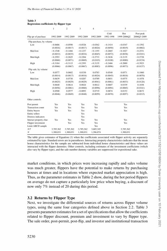
Table 3Regression coefficients by flipper type
1 2 3 4 5
Cold Hot Post peakFlip qtr of purchase 1992-2009 1992-2009 1992-2009 1992-2009 1992-1998 1999-2006Q2 2006Q3-2009
Flip purchase, by volumeLow −0.0686 −0.0590 −0.0526 −0.0362 −0.1414 −0.0347 −0.1592
(0.0016) (0.0017) (0.0017) (0.0024) (0.0050) (0.0019) (0.0062)Med-low −0.1548 −0.1466 −0.1237 −0.1193 −0.2665 −0.1027 −0.2531
(0.0032) (0.0035) (0.0034) (0.0045) (0.0072) (0.0038) (0.0101)Med-high −0.2593 −0.2625 −0.2204 −0.2733 −0.3636 −0.2135 −0.2728
(0.0068) (0.0071) (0.0069) (0.0103) (0.0108) (0.0080) (0.0154)High −0.3184 −0.3115 −0.2393 −0.3135 −0.3466 −0.2880 −0.3923
(0.0066) (0.0067) (0.0067) (0.0083) (0.0096) (0.0073) (0.0157)Flip sale, by volume
Low 0.0577 0.0682 0.0330 0.0783 0.0540 0.0571 0.1060(0.0014) (0.0017) (0.0016) (0.0024) (0.0045) (0.0018) (0.0070)
Med-low 0.0639 0.0730 0.0287 0.0789 0.0651 0.0575 0.1078(0.0025) (0.0029) (0.0029) (0.0041) (0.0061) (0.0033) (0.0126)
Med-high 0.0640 0.0614 0.0024 0.0612 0.0607 0.0339 0.1038(0.0056) (0.0061) (0.0060) (0.0096) (0.0094) (0.0065) (0.0341)
High 0.0500 0.0577 −0.0093 0.0719 0.0874 0.0153 0.0672(0.0046) (0.0049) (0.0048) (0.0059) (0.0070) (0.0057) (0.0215)
Other controls:
Post permit Yes Yes Yes Yes YesTransaction count Yes Yes Yes Yes YesEntity buyers Yes Yes Yes Yes YesEntity sellers YesDistress indicators YesInteract property char. Yes Yes Yes Yes YesFlipper investment Yes Yes Yes YesLimit ABCD sample YesNT 3,785,362 3,785,362 3,785,362 3,685,345 3,785,362N 1,300,031 1,300,031 1,300,031 1,286,874 1,300,031
The table gives estimates of Equation (1) when the coefficients associated with flipper activity are separatelyestimated by type. Standard errors are in parentheses. Interacting property characteristics indicates that the meanhouse characteristics for the sample are subtracted from individual house characteristics and these values areinteracted with the flipper dummies. Other controls, including estimates of the investment coefficients (whichalso vary by flipper type), and the sale number dummy variables are suppressed for expositional sake.
market conditions, in which prices were increasing rapidly and sales volumewas much greater, flippers have the potential to make returns by purchasinghouses at times and in locations where expected market appreciation is high.Thus, as the parameter estimates in Table 2 show, during the hot period flipperson average do not capture a particularly low price when buying, a discount ofnow only 7% instead of 20 during this period.
3.2 Returns by Flipper TypeNext, we investigate the differential sources of returns across flipper volumetypes, using the same four categories defined above in Section 2.2. Table 3presents parameter estimates for a set of specifications that allow the coefficientsrelated to flipper discount, premium and investment to vary by flipper type.The sale order, post-permit, post-flip, and investor and institutional transaction
5230
Dow
nloaded from https://academ
ic.oup.com/rfs/article/33/11/5212/5816604 by D
uke University user on 10 February 2021

[23:02 27/9/2020 RFS-OP-REVF200046.tex] Page: 5231 5212–5247
Speculators and Middlemen
dummy variables, and interactions of property characteristics are included inthe specifications reported in Table 3, but the parameter estimates (which aresimilar to those reported in Table 2) are not reported for ease of exposition. Thepost-flip controls and property characteristics are also interacted with flippertype to account for possible differences between types in the average investmentlevel and property attribute selection, respectively.
Our main result, seen in the basic specification in Column 1 and our preferredaugmented method in Column 2, is a striking heterogeneity in the sourcesof returns across flipper types. While all flippers buy below expected marketprice, higher-volume flippers buy at a much deeper discount relative to expectedmarket prices. For the whole sample period, the highest volume flippers receivea discount at purchase of approximately 31% compared to 6% for the lowestvolume types. Across specifications, discounts are monotonically increasingin volume type. Sales premiums are comparatively smaller and more similaracross types.
Column 3 adds indicators for entity sellers. This preserves the orderingof discount size across type but diminishes the magnitude for the highestvolume types. This indicates that, to some extent, the highest volume types earndiscounts by buying from nonoccupant sellers, who presumably have greaterholding costs. In Section 5.3 we examine the implications this propensity hasfor market liquidity. We leave out these effects for our headline calculationsbut bear them in mind for interpretation.
Column 4 limits the sample to properties satisfying both ends of theABCD restriction, showing the striking heterogeneity is robust to the moststringent specification controlling for physical investment. Finally, specification5, spanning three columns, separately estimates the flipper type purchase andsale dummies by time period. Discounts are larger for all flipper types duringcold market periods, though the heterogeneity between types is still evident. Thehigher-volume flippers exhibit the smallest differences in discounts betweencold and hot market periods. Steep discounts at the time of purchase areconsistent with these flippers operating as middlemen, finding properties to buycheaply and operating during any market conditions. Low-volume flippers, onthe other hand, generally do not buy at much of a discount, especially in hotmarket conditions. Like their cyclical purchase activity shown in Figure 3, thisis consistent with the idea that they are generally seeking to profit from marketappreciation as speculators rather than arbitraging as middlemen.26
Using the results from the estimates of specification 2 in Table 3, we canreport the source of a flipper’s return for each flipper type: decomposing thefraction that stems from buying cheaply, selling high, and simply earning the
26 The reduction in discounts during the hot period is a function of a compression of the dispersion in pricesduring periods of greater appreciation, but for low-volume flippers, of their buying closer to the center of thedistribution during the hot period. The behavior is consistent with a strategy of earning more return from marketappreciation, or at least, being less selective about finding “good deals” when the overall market in appreciating.Higher-volume flippers consistently buy at the lowest percentiles of the distribution at each place in the cycle.
5231
Dow
nloaded from https://academ
ic.oup.com/rfs/article/33/11/5212/5816604 by D
uke University user on 10 February 2021

[23:02 27/9/2020 RFS-OP-REVF200046.tex] Page: 5232 5212–5247
The Review of Financial Studies / v 33 n 11 2020
Table 4Sources of return by flipper type
1 2 3 4 5 6 7 8 9Volume Flips Buyer Seller Market Transaction Nominal Quarters Annualized Annualizedtype N discount premium growth cost rate of return held mkt growth rate of return
Low 49,660 −0.059 0.068 0.130 −0.104 0.153 4.074 0.127 0.150Med-low 17,892 −0.147 0.073 0.095 −0.112 0.202 3.151 0.120 0.256Med-high 5,473 −0.263 0.061 0.058 −0.123 0.259 2.388 0.097 0.434High 7,253 −0.312 0.058 0.037 −0.126 0.281 1.932 0.077 0.581
The table shows the sources of returns on flips by flipper type. The discounts, premiums, and market growth arecalculated from specification 2 of Table 3, and quarters held is simply the mean number of quarters held. Thegross rate of return is generated by totaling the sources of return, and the annualized return comes from dividingthe gross return by the mean years held. See the text for more details.
market return during the holding period. Table 4 provides these results. Weinclude estimates of flipper rates of return based on time held, market growth,and the residual transaction prices. Column 2 gives purchase discounts, Column3 the sale premiums, and Column 4 an estimate of market appreciation. We alsoinclude in Column 5 an estimate of transaction costs typically associated withthe buying and selling of real estate, including broker fees, deed recordingand local tax costs, and loan procurement (weighted by the probability thata loan is used to finance the transaction). The table consolidates all of theseinto one column for brevity, and we explain our computation of these costsin Appendix 5.27 Higher-volume types exhibit slightly larger transaction costsmostly because broker fees at time of sale represent a larger fraction of theheavily discounted purchase price. Column 6 reports the sum of gross returns.28
The returns for high-volume types are nearly twice that of the lowest types,and essentially all of their return owes to purchase discounts. Furthermore,Column 7 shows a large disparity in the time held (recalling Table 1). High-volume flipper quickly resell their houses, whereas low-volume flippers holdthem almost twice as long. Besides indicating a difference in strategy, this hasimplications for magnitude of annualized rates of return, which are that muchlarger for high-volume types, and the market appreciation component occupiesa smaller share even at annualized rates.
Although it is interesting that higher-volume types earn higher returns onaverage (even in gross annualized rates), for the purpose of understanding theirrole in the functioning of the housing market, we find it most important that thesource of their returns is primarily the steep discounts they earn at purchase.That is, the decomposition in Table 4 highlights how flippers of different types
27 It is also important to keep in mind that investors may face capital gains taxes after selling a property, but reliablecomputation of such taxes is difficult for a variety of reasons. One consideration, in particular, is the possibilitythat capital gains taxes can be deferred if a “like-kind” asset is purchased within one-half a year (the 1031exception). We have found in our data that, unsurprisingly, higher-volume flippers are more likely to purchaseagain in this window, at a rate of 65% compared to 18 recent among low-volume flippers, which, all else equal,would further separate their effective returns.
28 We say “gross returns,” distinct from net, to emphasize that we do not have measures of holding costs, costs ofcapital, or tax liability.
5232
Dow
nloaded from https://academ
ic.oup.com/rfs/article/33/11/5212/5816604 by D
uke University user on 10 February 2021

[23:02 27/9/2020 RFS-OP-REVF200046.tex] Page: 5233 5212–5247
Speculators and Middlemen
and roles find their returns from different sources, and provides strong evidencethat some flippers act as speculators while others operate as middlemen. Low-volume flippers do not buy at an especially low price and, as a result, their grossrate of return is primarily driven by overall market growth: 84% of their returnstems from market growth. High-volume flippers, on the other hand, earn mostof their return by buying at prices below average market prices and quicklyreselling so that only a small fraction (13%) of their return stems from overallmarket growth, whereas purchasing cheaply generates 54% of their return.
Taken together, the evidence on purchase activity, holding times, and sourcesof returns paints a very consistent picture: high-volume flippers generallyact as middlemen and low-volume flippers as speculators. We now establish(a) the robustness of these results to a number of potential concerns and(b) the external validity of the findings by demonstrating that the patternsdocumented so far for Los Angeles are also evident in many other U.S.cities.
3.3 RobustnessIn this subsection we summarize the analyses we have carried out to establishthe robustness of the results presented above to a number of the assumptionsthat underlie our analysis. To help with exposition we present the full detailsof the analyses in Appendix 6.
We begin by focusing on the definition of a flip and a flipper. In Appendix 6.1we show that our results are robust to other sensible definitions. For example,we show that the results are consistent whether flips are identified by buyershaving at least two short tenured-sales or as second homes. We also showthat the results are robust to other filters meant to address our misclassifyingtwo different people as the same investor if they share a common name. Wedemonstrate similar robustness if we restrict our identification of a flipperbased on the geography over which we allow them to operate (i.e., how farapart two transactions are allowed to be for the same flipper), or the maximumlength of time between transactions. In summary, while our identification offlippers may be imperfect, the primary result of the heterogeneity of returns byvolume type holds up to alternative definitions. Indeed, it would be remarkableif such a stark pattern were somehow the result of using buyer names toidentify investors. Improper aggregation should result in owner-occupiersbeing designated flippers, and low-volume flippers being designated as highervolume, and so on, which should homogenize the types and attenuate theestimates, the opposite of our findings.
In the results above, to focus on properties turned over quickly rather thanretained for rental income, we examined the sources of returns for houses thatwere resold in less than 2 years. Of course, the timing of the decision to resellthe property is an endogenous choice made by the investor, likely influenced bythe appreciation of the property and the cost of capital. By limiting the sample toonly those homes that were resold in the first 2 years, we may be inadvertently
5233
Dow
nloaded from https://academ
ic.oup.com/rfs/article/33/11/5212/5816604 by D
uke University user on 10 February 2021

[23:02 27/9/2020 RFS-OP-REVF200046.tex] Page: 5234 5212–5247
The Review of Financial Studies / v 33 n 11 2020
focusing on a selected sample of homes that performed well in terms of marketappreciation. Appendix 6.2 shows that our result that high- and low-volumeflipper types pursue different strategies is not sensitive to alternative restrictionson how fast a home must be resold to count as a flip.
As we discussed in detail above, a broad challenge in examining the sourcesof flipper returns is the possibility that flippers invest significant amounts ofmoney to improve properties, investment that is unobserved by the researcher.While several aspects of our baseline analysis have been designed to minimizethis concern, we further pursue this possibility in Appendix 6.3. We show thatif we further limit the time between sales at points A and B, and C and D,so as to minimize the possibility of unobserved investment, our results remainunchanged.29
For our baseline results, we estimated a single housing price index for theLos Angeles metropolitan market and used that to measure the rate of marketappreciation while flippers held on to properties, as reported in Table 4. An issuewith using a single aggregate price index for our analysis is that flippers mightbe able to identify and target submarkets or neighborhoods that appreciate fasterthan the metropolitan area as a whole. In one sense, this is not a problem but amatter of interpretation, as the submarket targeting might be the means by whichvolume flippers act as middlemen. But as a matter of measurement, it mightlead to an understatement of market appreciation and an overstatement of theexcess returns component of flipper returns. In Appendix 6.4 we show that ourresults are robust to alternative approaches for estimating “neighborhood-level”price indices.
Finally, we show in Appendix 6.5 that our results are not based on identifyingheterogeneous flipper types based on volume or experience. Rather, we showthat these types are persistent throughout a flipper’s tenure. For example,we show that even on their first two houses flipped, high-volume flippersreceived substantial discounts at purchase. Across flipper types, purchasediscounts and sales premiums are remarkably consistent throughout their careerprofile.
4. External validity: Flippers in other U.S. metro areas
We focus our analysis on Los Angeles, a large, diverse, and volatile housingmarket, for which there is available a long transaction record with which toconduct our analysis. To demonstrate the external validity of these results, inthis section we show the patterns of flipper behavior that we documented forLos Angeles are evident in many other U.S. metro areas.
29 Nothing in our analysis implies that flippers do not purchase fixer uppers that could be physically improved in aprofitable way. Rather, our research design ensures that such properties do not contribute to the identification ofthe sources of flipper returns that stem from buying cheaply and selling at a premium.
5234
Dow
nloaded from https://academ
ic.oup.com/rfs/article/33/11/5212/5816604 by D
uke University user on 10 February 2021

[23:02 27/9/2020 RFS-OP-REVF200046.tex] Page: 5235 5212–5247
Speculators and Middlemen
We construct data on flips and flippers for as many other large metro areaspossible during the time period we study. Dataquick collected transactionregister and county tax assessor data from public records in most large countiesin the United States, although available time periods and reporting practicesvary somewhat from county to county. Notably, the state of Texas suppressestransaction prices, so we exclude Texan cities from our analysis. Dataquick wasexpanding collection areas throughout the 1990s, and many metro areas do notcome online until late in the decade. Our identification of flippers and flippertypes relies on observing an individual’s activity over a sufficiently long timeperiod, so we limit our analysis to cities with continuous coverage as of 1998.We focus on larger metro areas, which we define as those with at least 100,000households (in the 2010 census) and an average of 500 transactions per quarterover its coverage period. For years after 1998, our sample totals 96 differentU.S. metro areas besides Los Angeles . See Appendix Table 74 for a list.
For the sake of exposition, in this analysis and for the rest of the paper wegroup flippers into two categories based on experience. High-volume flippers,or middlemen, are those who engage in three or more flips over our sample (inthe language above, these are medium-low, medium-high, and high) and low-volume flippers, or speculators, are those who flip two or fewer times during oursample. Given the findings above, this categorization divides flippers accordingto two distinct investment strategies.
Figure 4 shows the summary of flipper activity in our national sample ofmetro areas excluding Los Angeles. It displays the purchases by flipper type asa share of total transaction volume, pooling across all metro areas with availabledata in the quarter.30 The figure shows that both types of flippers are operatingnationally in ways largely similar to the Los Angeles market. Speculatorssharply increase their purchasing during the housing boom, while middlemenoperate at similar volumes throughout the cycle. Although investors’ shares oftransactions elsewhere are, on average, a bit lower than in Los Angeles, theirpresence is still sizable, and as we will show, the patterns of returns that wedocumented in Los Angeles will be apparent nationally.
As the level of activity by each flipper type varies across cities, we explorethe connections between their participation and features of the local housingin Appendix 7. The results from that analysis show that speculators operate athigher rates in markets with greater turnover in the housing market. Middlemenshow a much weaker association to transaction rates. We also show thatspeculator activity is higher in markets with greater price appreciation, whilemiddlemen exhibits a weaker correlation.31 These findings indicate that thecharacterization of speculators and middlemen from the Los Angeles market is agood depiction of their behavior more generally. Speculators operate cyclically
30 A separate series shows the number of metro areas in the sample at each quarter. By our criteria, this numberreaches its maximum of 96 in the year 1998.
31 This finding is in line with that of Adelino, Schoar, and Severino (2017).
5235
Dow
nloaded from https://academ
ic.oup.com/rfs/article/33/11/5212/5816604 by D
uke University user on 10 February 2021

[23:02 27/9/2020 RFS-OP-REVF200046.tex] Page: 5236 5212–5247
The Review of Financial Studies / v 33 n 11 2020
Figure 4Speculator and middlemen buying activity nationallyCalculations exclude the greater Los Angeles market and cities without sufficient transactions data as describedin main text.
in the national time series as well as being more prevalent in the marketswith more pronounced cyclical activity, while middlemen operate counter- oracyclically in the time series and in the cross section.
One of the key differences we highlighted between speculators andmiddlemen in Los Angeles was the source of their returns; namely thatmiddlemen purchase properties at a large discount relative to the market and incomparison to speculators. We now show that this pattern holds outside of LosAngeles. We reestimate Equation (1) for each metro area.32 This generates alarge number of buying and selling coefficients by flipper type, so we summarizethe results by presenting the distribution of point estimates in Figure 5. The leftpanel of Figure 5 shows that flippers of each type buy properties at substantialdiscounts,33 although the distribution of middlemen coefficients is clearly to theleft of the specul’tors’. The right panel shows that flippers earn small premiumsat the time of sale, and the average sale premiums earned by middlemen isslightly greater than that earned by speculators. For reference we label thepoint estimates for the Los Angeles market. Table 72 in Appendix 7 presentsestimates from a selection of notable markets. It is apparent that the patternof purchase discounts documented above for Los Angeles is common acrossseveral major cities, with Los Angeles itself near the center of the nationaldistribution. In Appendix 7 we relate the coefficient estimates for each city with
32 includeing Los Angeles, which we do, is not a redundant exercise, because the categorization of middlemen iscoarser than that of Table 3.
33 The results include a few cities with point estimates near or above zero, but none of the above-zero estimates arestatistically significant at the 5% level.
5236
Dow
nloaded from https://academ
ic.oup.com/rfs/article/33/11/5212/5816604 by D
uke University user on 10 February 2021
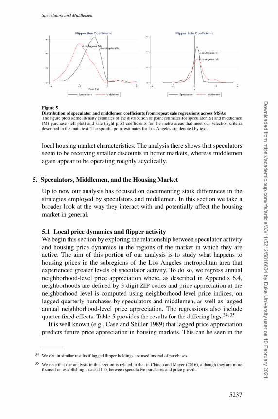
[23:02 27/9/2020 RFS-OP-REVF200046.tex] Page: 5237 5212–5247
Speculators and Middlemen
Figure 5Distribution of speculator and middlemen coefficients from repeat sale regressions across MSAsThe figure plots kernel density estimates of the distribution of point estimates for speculator (S) and middlemen(M) purchase (left plot) and sale (right plot) coefficients for the metro areas that meet our selection criteriadescribed in the main text. The specific point estimates for Los Angeles are denoted by text.
local housing market characteristics. The analysis there shows that speculatorsseem to be receiving smaller discounts in hotter markets, whereas middlemenagain appear to be operating roughly acyclically.
5. Speculators, Middlemen, and the Housing Market
Up to now our analysis has focused on documenting stark differences in thestrategies employed by speculators and middlemen. In this section we take abroader look at the way they interact with and potentially affect the housingmarket in general.
5.1 Local price dynamics and flipper activityWe begin this section by exploring the relationship between speculator activityand housing price dynamics in the regions of the market in which they areactive. The aim of this portion of our analysis is to study what happens tohousing prices in the subregions of the Los Angeles metropolitan area thatexperienced greater levels of speculator activity. To do so, we regress annualneighborhood-level price appreciation where, as described in Appendix 6.4,neighborhoods are defined by 3-digit ZIP codes and price appreciation at theneighborhood level is computed using neighborhood-level price indices, onlagged quarterly purchases by speculators and middlemen, as well as laggedannual neighborhood-level price appreciation. The regressions also includequarter fixed effects. Table 5 provides the results for the differing lags.34,35
It is well known (e.g., Case and Shiller 1989) that lagged price appreciationpredicts future price appreciation in housing markets. This can be seen in the
34 We obtain similar results if lagged flipper holdings are used instead of purchases.
35 We note that our analysis in this section is related to that in Chinco and Mayer (2016), although they are morefocused on establishing a causal link between speculative purchases and price growth.
5237
Dow
nloaded from https://academ
ic.oup.com/rfs/article/33/11/5212/5816604 by D
uke University user on 10 February 2021

[23:02 27/9/2020 RFS-OP-REVF200046.tex] Page: 5238 5212–5247
The Review of Financial Studies / v 33 n 11 2020
Table 5Flipper activity and local price dynamics
1 2 3 4 5
Price appreciation 0.197 −0.122 −0.186 −0.182 −0.134(0.0203) (0.0209) (0.0216) (0.0247) (0.0333)
Purchases by:Speculators 1.736 1.928 0.321 −1.784 −1.950
(0.2161) (0.2239) (0.2315) (0.2339) (0.2444)Middlemen −0.459 −0.465 −0.741 −0.397 0.283
(0.1608) (0.1673) (0.1737) (0.1742) (0.1805)
Obs 2,366 2,262 2,158 2,054 1,950R2 .8621 .8613 .8628 .8681 .8641Lags 1 2 3 4 5
The table shows regressions of neighborhood yearly price appreciation on quarterly speculator and middlemenpurchase activity and neighborhood-level yearly price appreciation. Each specification lags the covariates adifferent amount, which is given in the last row of the table.
top row of Table 5, which establishes positive short-term persistence and long-term mean reversion in house price appreciation at the neighborhood level.36
However, purchase activity of speculators is also associated with future priceappreciation. The first three columns show that a greater number of purchasesby inexperienced, speculative flippers are correlated with above average ratesof price appreciation over the following 2 years, moderating in the third, whilethe last two columns show that these short-term gains are followed by belowaverage returns over the following 3 years.
Middlemen, on the other hand, operate in areas where prices are risingmore slowly than the rest of the metropolitan area, and so their activity is notpredictive of future prices. Because middlemen primarily earn their returns byfinding “good ”eals” when purchasing and selling for high prices relative to themarket, it is not surprising to find them operating in hot and cold neighborhoods,just as they operate in hot and cold portions of the housing cycle.
5.2 How well informed are speculators?The evidence presented so far establishes that a substantial number of amateurspeculators entered the market in the recent housing boom and that their entryinto a submarket was associated with the formation and bursting of market-wideand local price bubbles over the next several years. In this subsection, we askwhether the fact their purchases are associated with future price appreciationin the short- to medium-term reflects their ability to predict and take advantageof short-term price spikes due to superior information about local marketfundamentals. If not, and speculators do not transmit valuable information tothe market or act with any special knowledge about market fundamentals, thentheir participation in and of itself may not improve market efficiency, and theiractivity may have, in and of itself, further fueled the mispricing in the housing
36 To our knowledge, the fact that, even at the neighborhood level, lagged appreciation strongly predicts future priceappreciation is undocumented elsewhere in the literature.
5238
Dow
nloaded from https://academ
ic.oup.com/rfs/article/33/11/5212/5816604 by D
uke University user on 10 February 2021

[23:02 27/9/2020 RFS-OP-REVF200046.tex] Page: 5239 5212–5247
Speculators and Middlemen
sector.37 Other ways that they may have improved the market’s functioninginclude providing liquidity and improving the capital stock through investment,and we also will investigate these possibilities below in Sections 5.3 and 5.4.
While some might take the inexperience of the speculators in the data asprima facie evidence that they are not especially well informed, we offer amore formal analysis of their behavior in this subsection.38 In particular, wepresent evidence from the timing of purchases and sales as the Los Angelesmarket neared and went over its peak in 2006 that suggests that flippers, andspeculators in particular, failed to anticipate the market’s peak in any way.
We think it is especially important39 to evaluate speculators vis-a-vismiddlemen on this front because they were so reliant on market timing. Thatspeculators could not anticipate the peak makes it difficult to rationalize thetiming and location of their activity as being driven by superior informationand instead makes it more likely that the causation could run in the oppositedirection.40 Of course, price appreciation and speculator participation may havebeen jointly influenced by other factors, such as a loosening in overall lendingstandards, and, in this paper, we do not provide evidence to the contrary. Fornow, our goal is to explore whether speculators were particularly well informedabout market fundamentals.
For the following analysis we construct a sample of all homes purchased byeach type of flipper, regardless of how long the property was eventually held,and for comparison, we include a measure of purchasing activity for owner-occupants. To display all on the same scale, we normalize the quarterly purchasevolume by the average quarterly purchases in 1998, the last year of the coldmarket, so that a value of one means at the 1998 average. Figure 6a plots theresultant indices for each type of buyer. The figure includes a shaded regiondenoting the period of greatest 2-year appreciation as the “hottest” period. Aflip held for 8 quarters would yield the greatest level of market appreciation ifpurchased at the start of this band and sold at its conclusion, and thus providesa rough guide of the beginning of the end of ideal market timing for a flipper.
The figure shows the substantial increase in speculator purchasing as pricesrose. Their level of activity in 2005 was 2.5 times that of 1998. That middlemenand owner occupiers showed little increase in activity indicates that much of
37 Our analysis in this subsection is similar in spirit to that of Griffin et al. (2011), who study the activity ofinstitutional and individual investors around the peak of the dot-com bubble.
38 Other researchers (e.g., Greenwood and Nagel 2009) have found that inexperienced traders engage in the typeof trend chasing behavior exhibited here. A multitude of evidence of this phenomenon hails from lab and retailinvestor survey settings. See, for example, Smith, Suchanek, and Williams (1988), Haruvy, Lahav, and Noussair(2007), or Vissing-Jorgensen (2003).
39 See also DeFusco, Nathanson, and Zwick (2017).
40 Our conclusion that speculators may have helped fuel the bubble is consistent with and complements the evidencepresented in Chinco and Mayer (2016), who develop a research design that makes use of data from multipleMSAs to identify the impact of long-distance investors on metropolitan price bubbles.
5239
Dow
nloaded from https://academ
ic.oup.com/rfs/article/33/11/5212/5816604 by D
uke University user on 10 February 2021
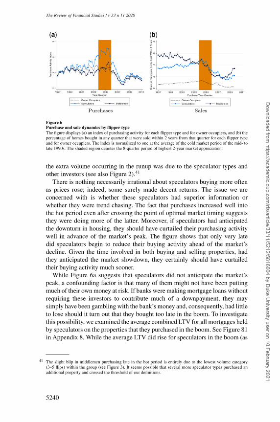
[23:02 27/9/2020 RFS-OP-REVF200046.tex] Page: 5240 5212–5247
The Review of Financial Studies / v 33 n 11 2020
(a) (b)
Figure 6Purchase and sale dynamics by flipper typeThe figure displays (a) an index of purchasing activity for each flipper type and for owner occupiers, and (b) thepercentage of homes bought in any quarter that were sold within 2 years from that quarter for each flipper typeand for owner occupiers. The index is normalized to one at the average of the cold market period of the mid- tolate 1990s. The shaded region denotes the 8-quarter period of highest 2-year market appreciation.
the extra volume occurring in the runup was due to the speculator types andother investors (see also Figure 2).41
There is nothing necessarily irrational about speculators buying more oftenas prices rose; indeed, some surely made decent returns. The issue we areconcerned with is whether these speculators had superior information orwhether they were trend chasing. The fact that purchases increased well intothe hot period even after crossing the point of optimal market timing suggeststhey were doing more of the latter. Moreover, if speculators had anticipatedthe downturn in housing, they should have curtailed their purchasing activitywell in advance of the market’s peak. The figure shows that only very latedid speculators begin to reduce their buying activity ahead of the market’sdecline. Given the time involved in both buying and selling properties, hadthey anticipated the market slowdown, they certainly should have curtailedtheir buying activity much sooner.
While Figure 6a suggests that speculators did not anticipate the market’speak, a confounding factor is that many of them might not have been puttingmuch of their own money at risk. If banks were making mortgage loans withoutrequiring these investors to contribute much of a downpayment, they maysimply have been gambling with the bank’s money and, consequently, had littleto lose should it turn out that they bought too late in the boom. To investigatethis possibility, we examined the average combined LTV for all mortgages heldby speculators on the properties that they purchased in the boom. See Figure 81in Appendix 8. While the average LTV did rise for speculators in the boom (as
41 The slight blip in middlemen purchasing late in the hot period is entirely due to the lowest volume category(3–5 flips) within the group (see Figure 3). It seems possible that several more speculator types purchased anadditional property and crossed the threshold of our definitions.
5240
Dow
nloaded from https://academ
ic.oup.com/rfs/article/33/11/5212/5816604 by D
uke University user on 10 February 2021

[23:02 27/9/2020 RFS-OP-REVF200046.tex] Page: 5241 5212–5247
Speculators and Middlemen
it also did for traditional home buyers), it remained around 90% at the peak, andwas at a rate comparable to that of traditional homebuyers.42 Thus, speculatorswere still putting a significant amount of their own money at risk and certainlyhad a financial incentive to stop making new purchases ahead of the peak.
The dynamics of flipper selling activity provides further evidence that theydid not anticipate the market peak. Figure 6b shows the fraction of homespurchased by speculators, middlemen, and owner occupiers in each quarterthat were sold within 2 years from that quarter. Not only did prices declinerapidly starting in 2006, but transaction volume had slowed considerably bylate 2005, making it difficult to unload any remaining inventory.
The figure indicates that, of the homes that were purchased prior to thesecond quarter of 2004, speculators typically sold 40% to 50% within 2 yearsof purchase, and middlemen 50 to 60. However, starting with homes purchasedin the second quarter of 2004, 2 years prior to the price peak, this percentagedeclined, tipping drastically as transaction volumes contracted. If speculatorshad anticipated the market peak, we would have expected them to have solda much greater percentage of the homes that they purchased in that quarter of2004, for example, within 2 years in order to avoid holding inventory as pricesfell precipitously. Instead, they were left with their holdings.
The pattern is not confined to speculators, however, as middlemen and owneroccupiers were similarly left with purchases made later in the cycle, indicatingthat none of these buyers unloaded inventory in anticipation of a market turn.Note however that Figure 6b conditions on purchase. That is, if speculatorsdemonstrated less-than-average prescience, it was in their elevated purchasesthrough the market peak, not in their propensity to sell holdings already ininventory.
5.3 Flippers and liquidityEven if speculators were uninformed market participants, they may haveimproved the housing market’s functioning by increasing overall liquidity. Inthis subsection we investigate this possibility. Specifically, we look at the partiesfrom whom the flippers are buying, and in particular, whether they are morelikely than an average homeowner to purchase a property not in use (held by aninstitution like a bank or government entity or one that has been foreclosedon). Table 6 reports the probability that the flipper’s purchase transactionindicated a seller we could identify via name text as a financial company(primarily banks), a government sponsored enterprise (Fannie Mae or FreddieMac), or a government entity like Housing and Urban Development (HUD)or state, county, or municipal governments. Finally, we also report purchases
42 Figure 81 also shows some interesting heterogeneity in how flippers use financing . Middlemen buying in coldmarkets are much more likely to pay cash than speculators, but conditional on purchasing during the hottestmarket period, they used loans at similar rates. Throughout, conditional on using a loan, they exhibit slightlyhigher rates of LTV than speculators or owner occupants.
5241
Dow
nloaded from https://academ
ic.oup.com/rfs/article/33/11/5212/5816604 by D
uke University user on 10 February 2021

[23:02 27/9/2020 RFS-OP-REVF200046.tex] Page: 5242 5212–5247
The Review of Financial Studies / v 33 n 11 2020
Table 6Probability of purchasing distressed properties
Buyer type: Owner- Other Flippers
Period Seller type occupier investors Speculators Middlemen
Purchases, 1992-2009N 2,748,701 262,692 155,766 94,341Bank/financial Co. 6.25 7.02 7.36 12.35Government entity 2.54 3.04 4.51 9.84GSE 2.26 2.21 2.46 4.03Foreclosed property 11.99 15.07 16.03 26.64
Cold: 1992-1998, 2006Q3-2009N 1,401,335 132,708 64,283 43,944Bank/financial Co. 10.53 12.15 14.27 20.00Government entity 3.10 3.51 5.87 10.95GSE 3.88 3.84 5.07 7.32Foreclosed property 17.71 22.69 25.94 36.79
Hot: 1999-2006Q2N 1,347,366 129,984 91,483 50,397Bank/financial Co. 1.80 1.78 2.50 5.67Government entity 1.95 2.56 3.56 8.87GSE 0.59 0.55 0.64 1.17Foreclosed property 6.04 7.30 9.07 17.78
The table reports the mean probabilities of the observed groups, by column, of conducting the action denoted ineach row. All figures, except sample counts, are expressed as percentages (%). “GSE” refers to a government-sponsored enterprise, namely, Fannie Mae or Freddie Mac.
of properties that we identify as being previously foreclosed up, meaning weobserve an institution taking ownership of the deed from a previous arm’s-length buyer, even if the institution is not observed as the seller of record (theforeclosure designation may overlap with institutional seller designations).43
Speculators make purchases of institutionally held properties slightly moreoften than owner occupiers and other investors. Middlemen, however, are abouttwice as likely to take part in these distressed transactions. The levels of thesepurchases rise during cold market periods, comprising a substantial fractionof middlemen’s purchases. This fact is consistent with the role of middlementaking properties off the market from high-holding-cost parties and providingliquidity, especially during downturns.
5.4 Flippers and investmentAnother way that speculators could improve the housing market is if theyimprove the overall capital stock by investing in the properties they flip. Toinvestigate this possibility, we use the assessor’s data to measure the rate ofpermit issuance during the holding period of the flippers. This is an imperfectmeasure of capital improvements. Sometimes permits are required for trivialmatters (to the market), and, likely more importantly, many market-valued
43 We use this definition to catch properties that move hands multiple times before we observe a market ratetransaction. The propensities are slightly smaller than when using Dataquick/Corelogic’s internal “distress sale”indicators, although qualitatively, the patterns by type of buyer hold with either definition.
5242
Dow
nloaded from https://academ
ic.oup.com/rfs/article/33/11/5212/5816604 by D
uke University user on 10 February 2021

[23:02 27/9/2020 RFS-OP-REVF200046.tex] Page: 5243 5212–5247
Speculators and Middlemen
Table 7Probability of improving properties and buying new or renovated properties
Buyer type Owner- Other Flippers
Period Purchase/action Type occupier investors Speculators Middlemen
Purchases, 1992-2009N 2,748,701 2,748,701 155,766 94,341Take permit 0.06 0.08 0.13 0.23Buy recent permit 2.83 2.33 1.96 1.29Buy from real estate developer 3.54 2.36 2.12 1.61Buy new construction 9.44 6.13 5.28 3.45
Cold: 1992-1998, 2006Q3-2009N 1,401,335 132,708 64,283 43,944Take permit 0.05 0.08 0.10 0.26Buy recent permit 3.38 2.72 2.31 1.47Buy from real estate developer 2.96 2.11 1.80 1.43Buy new construction 9.59 6.07 5.13 3.22
Hot: 1999-2006Q2N 1,347,366 129,984 91,483 50,397Take permit 0.07 0.08 0.14 0.20Buy recent permit 2.25 1.93 1.72 1.13Buy from real estate developer 4.14 2.63 2.35 1.77Buy new construction 9.28 6.18 5.38 3.64
The table reports the mean probabilities of the observed groups, by column, of conducting the action denoted ineach row. All figures, except sample counts, are expressed as percentages (%).
cosmetic improvements do not require the issuance of a permit. To this point,the flipper coefficients in the augmented repeat sales regressions (buy, sell, andpost-flip) help to capture things valued by the market, whether or not permitted.Moreover, from these regressions, the value of a property rises substantiallyafter issuance of a permit, on average about 13%. So despite its limitations,permit issuance seems a relevant feature to examine.
Table 7 reports the probability that the buyer is issued a permit during histenure of holding, a simple mean of the indicator variable and not adjustedfor holding length (i.e., not a hazard rate). This is a relatively rare occurrence,with less than one-half of a percent of holdings involving a permit issuance.44
Speculators are about twice as likely than owner-occupiers or other investorsto obtain a permit, but middlemen are roughly twice as likely as speculatorsand 4 times as likely as owner occupiers.45, 46 Moreover, the second and thirdpanels show that permit rates for middlemen are even higher during cold marketperiods—in contrast to speculators—suggesting that capital improvements area relatively larger part of their investment strategy.
The other rows of the table show that speculators are less likely than owneroccupiers or other investors to buy a recently permitted (i.e., recently renovated)
44 This is itself likely an undercounting of the true prevalence of permit issuance, because the assessor data isobserved once, so we only observe the most recent permit. For example, if an owner was issued a permit in 1995,and another owner of the property issued another permit in 2005, the data report only the 2005 permit.
45 Flipper rates are even higher as hazard rates, because flippers hold the properties for less time.
46 We note but do not report that that among middlemen, the rate of permit issuance rises with flipper volume.
5243
Dow
nloaded from https://academ
ic.oup.com/rfs/article/33/11/5212/5816604 by D
uke University user on 10 February 2021

[23:02 27/9/2020 RFS-OP-REVF200046.tex] Page: 5244 5212–5247
The Review of Financial Studies / v 33 n 11 2020
property, and less likely to buy new construction (as measured by sale andyear-built fields fewer than 2 years apart), or properties sold by real estatedevelopment companies (e.g., K Hovnanian). Middlemen are even less likelyto buy new or renovated structures. Hence, consistent with Table 13, flippers,but especially middlemen, are buying and selling older properties in greaterneed of rehabilitation.
6. Conclusion
Making use of a large transactions database and a novel research design, thispaper provides the first comprehensive study of intermediaries (middlemen andspeculators) in the housing market: identifying their activity, their sources ofthe returns and apparent strategies, the quality of their information with and theextent to which their activity affects liquidity and the overall stock of housing.
A main contribution of our analysis is a detailed characterization of the rolethat speculators played in the recent housing bubble. In particular, we documentsubstantial entry by amateur speculators at the height of the boom, entry thatwas strongly associated with sharp short-term increases and intermediate-termdeclines in local housing prices. Their collective inexperience and completeinability to anticipate the market peak by either curtailing their purchases orselling their inventory suggests that these speculators were not acting withsuperior information, but were instead simply betting that the boom wouldcontinue for a while longer.
Our analysis goes beyond a retelling of the role of speculation in the recentboom and bust. By examining the behavior of intermediaries over nearly aquarter century, we also identify real estate investors clearly operating in therole of middlemen. In this capacity, we document investors buying homes atprices well below market value and quickly reselling after short holding periodsat, or above, market value. These middlemen operate in all market conditionsand, if anything, are more active during busts, when the liquidity they provideto the market is likely to be especially valuable.
In this way, our analysis suggests that the impact of real estate investorson the market—especially whether their activity increases or decreases socialwelfare—likely depends critically on the market cycle. In busts, middlemenalmost certainly help to stabilize the market, effectively putting a floor on pricedeclines and providing liquidity for many homeowners who may be desperateto sell quickly following economic shocks. In booms, rampant speculation mayhave a de-stabilizing role that significantly amplifies price volatility. Even well-informed speculators may have deleterious effects on the market if they use theirinformational advantage to fuel and ride the bubble as in DeLong et al. (1990),although we find no such evidence of an informational advantage. Of course, anopen question is the extent to which our results extend to other settings wherethe goods are not durable like housing. We view this as a fruitful avenue forfuture research.
5244
Dow
nloaded from https://academ
ic.oup.com/rfs/article/33/11/5212/5816604 by D
uke University user on 10 February 2021

[23:02 27/9/2020 RFS-OP-REVF200046.tex] Page: 5245 5212–5247
Speculators and Middlemen
The possible contribution of real estate investors to a housing bubblehas led some policy makers to propose restrictions on their activity.47 Theappropriateness of such restrictions depends in part on the information contentof the speculation, and we provide evidence in this paper that speculators didnot, in fact, appear to be well informed of market fundamentals. Then again,such restrictions may inadvertently hamper the many welfare-enhancing rolesthat intermediaries play in markets that are subject to important search andinformational frictions. In particular, we also show that middlemen improvethe market’s liquidity and capital stock, and policies that impinge on theirbehavior may be welfare reducing. A crucial element to evaluating welfareeffects of flippers is the holding costs of sellers from whom they buy, a topicleft for future research.
While regulating investor behavior as a function of the market cycle maybe difficult, other policy tools may be available in the future. For example, bytracking investor activity as in our paper and Haughwout et al. (2011), it maybe possible to generate real-time measures of speculative activity based on datafrom housing transactions and mortgages. Such measures might provide anindication that a speculative boom was underway in a given market, providingthe just the kind of warning that was not widely available during the 2000s.
References
Adelino, M., A. Schoar, and F. Severino. 2017. Loan originations and defaults in the mortgage crisis: The roleof the middle class. Review of Financial Studies 29:1635–70.
Amihud, Y. and H. Mendelson. 1986. Asset pricing and the bid-ask spread. Journal of Financial Economics17:223–49.
Barberis, N. and R. Thaler. 2003. A survey of behavioral finance. In Handbook of the economics of finance, eds.G. Constantinides, M. Harris, and R. Stulz, vol. 1. Amsterdam, the Netherlands: Elsevier.
Bayer, P., K. Mangum, and J. W. Roberts. 2019. Speculative fever: Investor contagion in the housing bubble.Working Paper, Duke University.
Bhutta, N. 2015. The ins and outs of mortgage debt during the housing boom and bust. Journal of MonetaryEconomics 76:284–98.
Bostic, R., S. Gabriel, and G. Painter. 2009. Housing wealth, financial wealth, and consumption: New evidencefrom micro data. Regional Science and Urban Economics 39:79–89.
Brunnermeier, M. K. and S. Nagel. 2004. Hedge funds and the technology bubble. Journal of Finance59:2013–40.
Case, K. E. and R. J. Shiller. 1987. Prices of single-family homes since 1970: New indexes for four cities. NewEngland Economic Review Sept/Oct:45–56.
———. 1989. The efficiency of the market for single-family homes. American Economic Review 79:125–37.
47 For example, a 2006 HUD regulation (Federal Register, volume 71, p. 33,138) prevented FHA financing forhouses sold within 90 days of purchase. Partly in response to the weak housing market, HUD waived thisrestriction in 2010 (Federal Register, volume 75, p. 28,633). More broadly, antispeculative policy prescriptions,such as transaction taxes, have been suggested in other speculative markets. See, for example, Tobin (1974),Tobin (1978), Eichengreen, Tobin, and Wyplosz (1995), or Summers and Summers (1988).
5245
Dow
nloaded from https://academ
ic.oup.com/rfs/article/33/11/5212/5816604 by D
uke University user on 10 February 2021

[23:02 27/9/2020 RFS-OP-REVF200046.tex] Page: 5246 5212–5247
The Review of Financial Studies / v 33 n 11 2020
Cheng, I.-H., S. Raina, and W. Xiong. 2014. Wall street and the housing bubble. American Economic Review104:2797–829.
Chinco, A. and C. Mayer. 2016. Misinformed speculators and mispricing in the housing market. The Review ofFinancial Studies 29:486–522.
Copeland, T. E. and D. Galai. 1983. Information effects on the bid-ask spread. Journal of Finance 38:1457–69.
DeFusco, A. A., C. G. Nathanson, and E. Zwick. 2017. Speculative dynamics of prices and volume. WorkingPaper, University of Chicago.
DeLong, J. B., A. Shleifer, L. H. Summers, and R. J. Waldmann. 1990. Positive feedback investment strategiesand destabilizing rational speculation. Journal of Finance 45:379–95.
Demsetz, H. 1968. The cost of transacting. Quarterly Journal of Economics 82:33–53.
Eichengreen, B., J. Tobin, and C. Wyplosz. 1995. Two cases for sand in the wheels of international finance.Economic Journal 105:162–72.
Fama, E. F. 1965. The behavior of stock-market prices. Journal of Business 38:34–105.
Favilukis, J. Y. and S. Van Nieuwerburgh. 2018. Out-of-town home buyers and city welfare. Working Paper,University of British Columbia.
Gao, Z., M. Sockin, and W. Xiong. 2017. Economic consequences of housing speculation. Working Paper,Chinese University of Hong Kong.
Garber, P. M. 1989. Tulipmania. Journal of Political Economy 97:535–60.
Garman, M. B. 1976. Market microstructure. Journal of Financial Economics 3:257–75.
Glosten, L. R. and P. R. Milgrom. 1985. Bid, ask and transaction prices in a specialist market with heterogeneouslyinformed traders. Journal of Financial Economics 14:71–100.
Glower, M., D. R. Haurin, and P. H. Hendershott. 1998. Selling time and selling price: The impact of sellermotivation. Real Estate Economics 26:719–40.
Greenwood, R. and S. Nagel. 2009. Inexperienced investors and bubbles. Journal of Financial Economics 93:239–58.
Griffin, J. M., J. H. Harris, T. Shu, and S. Topaloglu. 2011. Who drove and burst the tech bubble? Journal ofFinance 66:1251–90.
Griffin, J. M. and G. Maturana. 2016. Who facilitated misreporting in securitized loans? Review of FinancialStudies 29:384–419.
Haruvy, E., Y. Lahav, and C. N. Noussair. 2007. Traders’ expectations in asset markets: Experimental evidence.American Economic Review 97:1901–20.
Haughwout, A., D. Lee, J. Tracy, and W. van der Klaauw. 2011. Real estate investors, the leverage cycle, and thehousing market crisis. Working Paper, Federal Reserve Bank of New York.
Kindelberger, C. P. 1978. Manias, panics and crashes: A history of financial crises. New York: John Wiley &Sons.
Kyle, A. S. 1985. Continuous auctions and insider trading. Econometrica 53:1315–35.
Mackay, C. 1841. Extraordinary popular delusions and the madness of crowds, 1932 edition. London: RichardBentley.
Mayer, C., K. Pence, and S. M. Sherlund. 2009. The rise in mortgage defaults. Journal of Economic Perspectives23:27–50.
Mian, A. and A. Sufi. 2014. What explains the 2007-2009 drop in employment? Econometrica 82:2197–223.
5246
Dow
nloaded from https://academ
ic.oup.com/rfs/article/33/11/5212/5816604 by D
uke University user on 10 February 2021

[23:02 27/9/2020 RFS-OP-REVF200046.tex] Page: 5247 5212–5247
Speculators and Middlemen
———. 2017. Fraudulent income overstatement on mortgage applications during the credit expansion of 2002to 2005. Review of Financial Studies 30:1832–64.
———. 2018. Credit supply and housing speculation. Working Paper, Princeton University.
Piazzesi, M. and M. Schneider. 2009. Momentum traders in the housing market: Survey evidence and a searchmodel. American Economic Review 99:406–11.
Piskorski, T., A. Seru, and J. Witkin. 2015. Asset quality misrepresentation by financial intermediaries: Evidencefrom the rmbs market. Journal of Finance 70:2635–78.
Rajan, R. and R. Ramcharan. 2015. The anatomy of a credit crisis: The boom and bust in farm land prices in theunited states in the 1920s. American Economic Review 105:1439–77.
Rognlie, M., A. Shleifer, and A. Simsek. 2018. Investment hangover and the great recession. American EconomicJournal: Macroeconomics 10:113–53.
Shiller, R. J. 2003. From efficient markets theory to behavioral finance. Journal of Economic Perspectives17:83–104.
Shleifer, A. and L. H. Summers. 1990. The noise trader approach to finance. Journal of Economic Perspectives4:19–33.
Smith, V. L., G. L. Suchanek, and A. W. Williams. 1988. Bubbles, crashes, and endogenous expectations inexperimental spot markets. Econometrica 56:1119–51.
Springer, T. M. 1996. Single-family housing transactions: Seller motivations, price, and marketing time. Journalof Real Estate Finance and Economics 13:237–54.
Spulber, D. F. 1996. Market-making by price setting firms. Review of Economic Studies 63:559–80.
Summers, L. H. and V. P. Summers. 1988. When financial markets work too well: A cautious case for a securitiestransactions tax. Journal of Financial Services Research 3:261–86.
Temin, P. and H.-J. Voth. 2004. Riding the south sea bubble. American Economic Review 94:1654–68.
Tobin, J. 1974. The new economics one decade older. Princeton, NJ: Princeton University Press.
———. 1978. A proposal for international monetary reform. Eastern Economic Journal 4:153–9.
Vissing-Jorgensen, A. 2003. Perspectives on behavioral finance: Does irrationality disappear with wealth?Evidence from expectations and actions. In NBER Macroeconomics Annual, eds. M. Gertler and K. Rogoff.Cambridge: MIT Press.
5247
Dow
nloaded from https://academ
ic.oup.com/rfs/article/33/11/5212/5816604 by D
uke University user on 10 February 2021