SpeedDating: An Algorithmic Case Study

involving Matching and Scheduling

Study Thesis of

Ben Strasser

At the faculty of Computer Science

Institute of Theoretical Informatics

Algorithmics I

Advisors: Dr. rer.-nat. Bastian Katz

Dipl.-Inform. Ignaz Rutter

Prof. Dr. Dorothea Wagner

Processing Time: 10. May 2010 � 19. August 2010

KIT � University of the State of Baden-Wuerttemberg and National Laboratory of the Helmholtz Association www.kit.edu

Hiermit erkläre ich, dass ich die vorliegende Arbeit selbstständig verfasst und die vorgestelltenErgebnisse ohne die Hilfe Dritter erarbeitet habe. Ich habe auf keine anderen als die angegebenenQuellen und Hilfsmittel zurückgegri�en.

Ben StrasserKarlsruhe, den 19. August 2010

Contents

1 Introduction 1

2 De�nitions 2

3 Problem description 2

3.1 Formal Speci�cation . . . . . . . . . . . . . . . . . . . . . . . . . . . . . . . . . . . 23.2 Integer Linear Program . . . . . . . . . . . . . . . . . . . . . . . . . . . . . . . . . 33.3 Classi�cation . . . . . . . . . . . . . . . . . . . . . . . . . . . . . . . . . . . . . . . 4

4 Algorithm for Heterosexual Speed Dating 5

4.1 Phase 1: Determine the Minimum fairness violation . . . . . . . . . . . . . . . . . 54.2 Phase 2: Determine the Maximum Weight Subgraph . . . . . . . . . . . . . . . . . 64.3 Phase 3: Coloring the Edges . . . . . . . . . . . . . . . . . . . . . . . . . . . . . . . 84.4 Analysis . . . . . . . . . . . . . . . . . . . . . . . . . . . . . . . . . . . . . . . . . . 9

5 Approximation Algorithm for Homosexual Speed Dating 10

5.1 Performance Guarantees . . . . . . . . . . . . . . . . . . . . . . . . . . . . . . . . . 115.2 Phase 2: Determine the Maximum Weight Subgraph . . . . . . . . . . . . . . . . . 125.3 Phase 3: Coloring the Edges . . . . . . . . . . . . . . . . . . . . . . . . . . . . . . . 145.4 Phase 4: Removing the Lightest Color . . . . . . . . . . . . . . . . . . . . . . . . . 145.5 Analysis . . . . . . . . . . . . . . . . . . . . . . . . . . . . . . . . . . . . . . . . . . 14

6 Heuristics 15

6.1 δ-absolute . . . . . . . . . . . . . . . . . . . . . . . . . . . . . . . . . . . . . . . . . 156.2 δ-initial . . . . . . . . . . . . . . . . . . . . . . . . . . . . . . . . . . . . . . . . . . 166.3 δ-relative . . . . . . . . . . . . . . . . . . . . . . . . . . . . . . . . . . . . . . . . . 16

7 Evaluation 17

7.1 Heterosexual Dating . . . . . . . . . . . . . . . . . . . . . . . . . . . . . . . . . . . 177.1.1 Varying the Number of People . . . . . . . . . . . . . . . . . . . . . . . . . 187.1.2 Varying the Number of Dates . . . . . . . . . . . . . . . . . . . . . . . . . . 197.1.3 Real World Scenario . . . . . . . . . . . . . . . . . . . . . . . . . . . . . . . 20

7.2 Homosexual Dating . . . . . . . . . . . . . . . . . . . . . . . . . . . . . . . . . . . . 217.2.1 Varying the Number of People . . . . . . . . . . . . . . . . . . . . . . . . . 217.2.2 Varying the Number of Dates . . . . . . . . . . . . . . . . . . . . . . . . . . 227.2.3 Real World Scenario . . . . . . . . . . . . . . . . . . . . . . . . . . . . . . . 23

8 Conclusion 23

1 Introduction

A speed dating event is an event where a number of people come together to date each other for ashort period of time. As dates can only involve two persons it is not possible that everybody dateseveryone at the same time. It is usually done by scheduling dating rounds such that in each roundevery person dates at most one other person.

Consider a group of six men and six women that attend such an event. To make sure thatevery man dates every woman and vice versa we need six rounds. Suppose that a round lasts tenminutes then the whole event will last at least one hour. Most likely it will last longer as peopleneed to change seats to get to the next date. With such a small group of people we can simplypair everyone with everyone. However, in larger groups such as 200 men and 200 women, the eventwould last about one and a half day. Hence, the organizers of such events need to make a selectionof dates in advance to limit the number of rounds.

One approach to tackle this problem is to make the participants �ll out forms about their idealpartner before the event. Based on this information it is possible to estimate in advance how wella certain date would work. We call this the quality of the date. We now select the pairings sothat the overall quality is maximized and no person has more dates than the maximum number ofrounds. This way we can cap the number of rounds to say twelve and the whole event will thenonly last between two and three hours.

There are however a couple of problems with this approach.

• Certain persons are more attractive than others and would get all of the dates leaving nonefor the less attractive ones. Distributing the dates in a fair way therefore is important.

• Generally there are more men than women on such events. The only way to manage this isto make every man miss a couple of turns.

• Some persons, which we call VIP-persons, may be more important than others because ofcertain circumstances. They might for example have paid extra money. Even though wegenerally try to be fair in distributing dates these persons clearly must be preferred. Weespecially want to make sure that these persons do not have to miss turns.

• People may not show up at the event even though they registered. The problem with this isthat all the people that were scheduled for this person will get one date less than planned ifthe planning can not be adjusted in time. The simplest way of solving this problem is simplynot to do any calculations in advance. The plan should be generated just before the eventstarts. This way the event organizers know who showed up. As one can not force the peopleto show up several hours before the event takes place these calculations must be �nishedwithin a couple of minutes.

So far we have only described heterosexual speed dating but one may also consider homosexualdating. In this setting we do not make a distinction between men and women. Every personmay date every other person. We can regard this as a generalization of the heterosexual datingproblem, where the dates between persons of the same sex have a very bad quality. We show thatthis generalization is a lot harder to solve.

In this thesis we develop algorithms to generate the dating rounds based on the data collectedusing the �lled forms. Each of these rounds consists of a list of pairings. We do not order theserounds in time nor do we try to optimize the time the people need to change their seats.

Selecting the dates is a matching problem and distributing them among the di�erent rounds is ascheduling problem. There are a few additional non-standard constraints on the matching to makesure that the dates are selected in a way that is fair for every person. We investigate whether thesetwo subproblems may be solved separately. It turns out that this is not possible when consideringhomosexual dating.

After we recalled a few basic de�nitions in Section 2 we formalize the generalized homosexualproblem setting and classify it in Section 3. It turns out that the problem is NP-hard. Weformulate the problem in graph-theoretic terms and as an integer linear program (ILP). Afterwardswe develop a polynomial-time algorithm for the heterosexual special case in Section 4. We thentry to generalize this algorithm and obtain a polynomial-time approximation algorithm with goodperformance guarantees in Section 5. This done, we investigate a couple of greedy heuristics tosolve the problems in Section 6. Finally we evaluate the performances of the algorithms describedby implementing them and applying them to random test data in Section 7.

1

2 De�nitions

We will use mostly standard notation for graph theory as de�ned by e.g. Diestel [5]. The mostimportant di�erence is that the induced subgraph of an edge set contains all nodes and not onlythose that are an end of some edge. We recall the most important terms.

A graph G is a tuple (V,E) where V is a �nite set called the set of nodes and E is a subsetof(V2

)called the set of edges. We denote the number of nodes with n and the number of edges

with m. The degree d(v) of a node v is the number of incident edges, i.e. , d(v) = |{e ∈ E | v ∈ e}|.The maximum degree over all nodes is denoted by 4G i.e. 4G = maxv∈V d(v). A subgraphof a graph G = (V,E) is itself a graph G′ = (V ′, E′) such that V ′ ⊆ V and E′ ⊆ E. Thedegree of a node in a subgraph is denoted by d′(v). Given an edge set E′ the graph (V,E′)is called the induced subgraph. A directed graph is a tuple (V,A) where V is a �nite node setand A ⊆ V × V \{(v, v) | v ∈ V } is the set of arcs.

A matching is an edge subset such that each node has at most degree one in the induced graph.A perfect matching is a matching where each node has a degree of exactly one. A matching ismaximum if no matching exists that contains more edges.

An edge coloring is a function that maps E onto a set of colors C such that all edges incidentto the same node are colored di�erently. We identify the colors with the numbers {1, 2, . . . , |C|}.A node misses a color if it has no incident edge of that color. The set of natural numbers N startswith zero, i.e., N = {0, 1, 2, . . .}.

3 Problem description

This section formalizes the homosexual dating problem and its heterosexual special case describedin the introduction. We �rst provide a problem statement in graph-theoretic terms. Then we modelthis problem as an ILP and we show that the general Speed Dating problem is NP-complete.

3.1 Formal Speci�cation

The people are represented using nodes and the potential dates as edges. We discard potentialdates with a very bad quality leading to a graph that is not necessarily complete. We refer to dateswith such a bad quality as bad dates. The graph G = (V,E) obtained in this way is simple andundirected. It does not have to be connected. The heterosexual special case provides a bipartitegraph structure since no woman dates any woman and no man dates any man.

We formalize the quality of a potential date using a non-zero natural number. A high valuedescribes a high quality whereas a value close to 1 means a second-rate date. This makes the graphweighted. VIP-persons can be given a boost by augmenting the weight on their outgoing edges.One goal is to maximize the sum of the weights of the selected dates. Another goal is to distributethe dates in a fair way.

To make sure that no person gets no dates just because he or she is unattractive, we set alower and an upper bound called ` and h for the number of dates that each person gets. Eachperson v has at most h(v) dates and if possible at least `(v) dates. In most situations one wouldset h(v) = `(v) but di�erentiating between both allows for more �exibility. Consider for examplea dating event with w women, m men, σ rounds and heterosexual dating. Let us recall that thereare less women than men. Then one could set `(v) = h(v) = σ for each woman resulting in a totalof wt dates. As this number can not always evenly be divided between all the men it thereforemakes sense to set `(v) = bwt/mc and h(v) = dwt/me. Figure 1 shows an example. VIP-personsmay be given a higher value for `(v) than other people. As one can see it makes sense to choosedi�erent bounds for di�erent people and in some cases even h(v) 6= `(v) makes sense.

Our primary objective is to select the dates in such a way that the ` and h bounds are met.This is however not always possible. If this is not the case then we lower ` for each person by 1euntil a solution exists. We call the value by which we have to lower ` the fairness violation δ. Inthe following ` always refers to the �xed optimal lower bound given as input and `− δ is the actuallower bound used. The smaller the violation δ is the better.

Each person v has d(v) potential dates and d′(v) dates that actually take place. As a conse-quence the following inequality holds:

0 ≤ `(v)− δ ≤ d′(v) ≤ h(v) ≤ d(v)

2

W

W

M

M

M

Figure 1: A possible selection of dates for two women, three men and two rounds. The solid linesare the selected dates. No matter what dates we select there will always be one man with twodates and two men with one date.

We can interpret d(v) as the degree of v in the given graph and d′(v) as the degree in the graphinduced by the selected dates. We can regard the search for these dates as a search for a sub-graph G′ = (V,E′) of G that ful�lls the given requirements on the node degrees.

A further restriction is that it must be possible to distribute the selected dates onto the di�erentrounds. In graph-theoretic terms this means that we must be able to color the selected dates usingat most σ colors, where σ is the number of turns. It turns out that this is the requirement thatcauses the homosexual version to be NP-hard.

Among the solutions that satisfy the conditions formulated and that have an optimal fairnessviolation we choose the solution with the maximum total weight. Now that we have formalized thedi�erent parts of the problem we are ready to state the speed dating problem.

Problem 1. Given a graph G = (V,E) with edge weights w : E → N\{0} and lower and uppernode capacities `, h : V → N such that for each vertex v the inequality `(v) ≤ h(v) ≤ d(v) holds,determine an edge subset colored with at most σ = maxv∈V h(v) colors. The degree d′(v) of eachvertex v in the induced subgraph should be smaller than h(v). The subgraph should be optimalwith regard to the following two criteria:

• Maximize the sum of the weights of the edges in the subgraph. We refer to this as the weightcriterion.

• Minimize the maximum di�erence δ between `(v) and d′(v). We call this di�erence fairnessviolation. More formally

δ = max(0,maxv∈V

`(v)− d′(v))

We refer to this criterion as the fairness criterion.

It is possible to look at this problem as a bicriterial one. However we �rst minimize the fairnessviolation δ. Among the smallest δ we choose the solution that maximizes the weight. It is thereforealways possible to determine whether a solution is better, worse or just as good as another one.

3.2 Integer Linear Program

The speed dating problem can be formulated as an integer linear program (ILP). We introducebinary decision variables xe,c ∈ {0, 1} that model the question if an edge e is colored using thecolor c. If xe,c = 1 then the edge e is colored using c. Further, we introduce two variables δ and srepresenting how well the fairness and weight criteria are met. Let us recall that C denotes the setof colors. The constraints of the program are:

3

∑{u,v}∈E

x{u,v},c ≤ 1 ∀u ∈ V, c ∈ C (1)

∑c∈C

xe,c ≤ 1 ∀e ∈ E (2)∑{u, v} ∈ Ec ∈ C

x{u,v},c ≤ h(u) ∀u ∈ V (3)

∑{u, v} ∈ Ec ∈ C

x{u,v},c ≥ `(u)− δ ∀u ∈ V (4)

δ ≥ 0 (5)

s =∑e ∈ Ec ∈ C

w(e)xe,c (6)

The constraint (1) ensures that all edges incident to the same node are colored di�erently. Theequation (2) makes sure that every edge is colored using at most one color, i.e., that no date takesplace more than once. An edge may be uncolored meaning that it is not selected. Inequality (3)ensures that the upper degree bound requirement is met for every node.

The constraints (4) and (5) measure how well the fairness criterion is met. Equation (6) does thesame for the weight criterion. These three last constraints are only needed to be able to formulatethe objective function. They do not in�uence which edge subsets are considered to be valid.

We can formulate the objective function using a large constant s.

s− δs = max!

Since s is needed to make sure that the fairness criterion dominates the weight criterion it mustbe at least as big as any value that s can possibly take. The total weight s is maximum if thesubgraph is the whole graph G, which leads us to a su�cient lower bound for s, namely

s ≥ 1 +∑

{u,v}∈E

w({u, v}) .

In Section 7 we evaluate the speed of a speed dating solver that is composed of this ILP problemformulation and an o�-the-shelf ILP solver. It is largerly outperformed by the solvers described inSections 4 and 5 which make use of combinatorial approachs.

3.3 Classi�cation

We have formalized the speed dating problem. A natural question to ask before trying to solve itis how hard it is. In this Section we prove that it is NP-complete.

Lemma 2. The speed dating problem is NP -hard.

Proof. Determining whether a graph G = (V,E) can be colored with exactly 4G colors is NP -hard [7]. Given an instance of this graph coloring problem we set w(e) = 1, `(v) = 0 and h(v) = d(v)for all e ∈ E and v ∈ V and obtain an instance of the speed dating problem with the propertythat σ = 4G. This transformation can be computed in polynomial time. Solving it yields acolored edge subset E′. As `(u) = 0 the fairness criterion is always satis�ed optimally and can beignored. As all edges have the same weight the speed dating problem tries to color as many edgesas possible. This means it determines a largest edge subset E′ that can be colored using 4G colors.A valid coloring of G exists if and only if E = E′. This implies that the speed dating problem isNP -hard.

Another natural question to ask is how hard the problem is.

4

Lemma 3. The decision problem corresponding to the speed dating problem is in NP .

Proof. We have to show that given two positive integers δ, s and an instance of the speed datingproblem one can determine whether a solution exists that is at least as good as δ with regard tothe fairness criterion and as s with regard to the weight criterion using only a deterministic Turingmachine with an oracle. First, the oracle guesses the solution and then the machine veri�es inpolynomial time whether it meets the requirements. Given a solution we can determine how goodthe fairness criterion is met by calculating the solution's δ using the formula given in the de�nitionof the problem and comparing it to the given δ. The weight criterion can be tested in a similarway by summing up the weights of the edges in the subgraph.

Combining Lemmas 2 and 3 shows that the speed dating problem is NP-complete. A con-sequence of this is that unless P = NP it is not possible to formulate the problem as a linearprogram.

4 Algorithm for Heterosexual Speed Dating

Before trying to solve the complete problem formulated in the previous section we �rst solve theheterosexual special case. Let us recall that in graph-theoretic terms this means that the inputgraph is bipartite. Our algorithm works in three phases.

1. Determine the minimum fairness violation δ using a binary search.

2. Determine the maximum weight uncolored edge subset E′ for a �xed δ. Denote with G′ theinduced graph.

3. Color the edge set determined in the second phase using 4G′ colors.

A key observation is that every bipartite graph can be edge colored e�ciently using 4G′ colors.We describe in Section 4.3 an algorithm that achieves this. As a consequence we can compute thePhases 1 and 2 completely independently from Phase 3. This degree of independence is howevernot given between the �rst two phases. Phase 1 makes use of the algorithm developed in Phase 2to check whether a solution exists given a �xed δ. Note that the solution is valid because 4G′ ≤maxv∈V h(v) = σ

4.1 Phase 1: Determine the Minimum fairness violation

Given a �xed fairness violation δ we can transform the problem instance into one where the lowernode capacities are tight bounds meaning that `(v) ≤ d′(v) must hold for each node v. Thetransformation is

`(v)← max{0, `(v)− δ}Once transformed the problem of �nding an uncolored edge set boils down to the weighted

degree constrained edge subset problem (WDCES), which can be stated as follows.

Problem 4 (WDCES). Given a graph G = (V,E) with edge weights w : E → N\{0}, lower andupper node capacities `, h : V → N such that for each node v the inequality `(v) ≤ h(v) ≤ d(v)holds, determine an edge set E′ with maximum weight such that `(v) ≤ d′(v) ≤ h(v) holdswhere d′(v) is the degree of the node v in the induced subgraph.

This problem is also known as b-matching with unit edge capacities. In Phase 2 we describean algorithm to solve this problem. Further a straightforward variation is described that testswhether any feasible uncolored edge subset exists. As the third phase can never fail it is su�cientto determine whether the speed dating problem with a �xed fairness violation δ has a solution. Itis important to note that at this point we exchange the variable δ in the original problem settingwith a �xed constant.

We make use of this variation to determine the minimum δ using a binary search. We knowthat δ is in the interval [0,maxv∈V `(v)] and that it is integral. Further, if no feasible solutionexists for a certain δ then none exists for smaller values either. If a solution exists then it is also asolution for all bigger values of δ. These are all the ingredients needed to determine the optimal δusing a binary search. We guess a δ and apply the feasibility test from Phase 2 to determine if it istoo small or big enough and adjust δ accordingly. See Algorithm 1 for some pseudo code showingthe details of this algorithm.

5

Algorithm 1 Algorithm to determine the optimal δ using a binary search

δmin ← 0;δmax ← maxv∈V `(v);while δmin 6= δmax do

δ ←⌊δmin+δmax

2

⌋;

for every vertex v do`′(v)← max(`(v)− δ, 0);

end

if phase 2 is feasible using `′ thenδmax ← δ;

elseδmin ← δ + 1;

end

end

The optimal δ is δmin

4.2 Phase 2: Determine the Maximum Weight Subgraph

This phase basically consists of solving the WDCES problem that was formulated in Section 4.1.Since we only consider bipartite graphs we can reduce it to the min cost �ow problem (MCF).Several versions of this problem exist. We will use the one described in the Lemon library [2] aswe want to make use of its implementation.

Problem 5 (MCF). Given a directed graph D = (VD, A) with arc costs c : A → R, lowerand upper arc capacities `D, hD : A → R such that `D(a) ≤ hD(a) for each arc a and a nodesupply q : VD → R �nd a �ow f : A→ R such that∑

a∈Ac(a)f(a) = min! (7)∑

(u,v)∈A

f(u, v)−∑

(v,u)∈A

f(v, u) ≥ q(u) ∀u ∈ V (8)

`D(a) ≤ f(a) ∀a ∈ A (9)

hD(a) ≥ f(a) ∀a ∈ A (10)

It has been shown that if a solution exists and `D, hD and q only take integral values then anoptimal solution exists where f also only takes integral values [3]. Lemon provides an algorithmthat solves this problem optimally. This algorithm �nds an integral �ow when c, `D and hD areintegral.

The supply model used here is more general than we will need. In our case we will have q(v) 6= 0only for two special nodes in D called the source node s and the target node t. We set q(s) = −q(t).The �ow has an amount of q(s), which we will denote by p. This self-imposed restriction allows usto rewrite (8) as the better known �ow conservation equation.

∀u ∈ VD\{s, t} :∑

(u,v)∈A

f(u, v) =∑

(v,u)∈A

f(v, u) (11)

It basically means that �ow can only be created or destroyed at the source and at the target,respectively. Equation (7) minimizes the cost the �ow causes along its way. The capacity con-straints (9) and (10) re�ect the node capacities of the weighted degree constrained subgraph prob-lem.

Min Cost Flow Reduction

Given a WDCES instance we can construct an equivalent MCF instance based on it. Let D be adirected graph whose nodes are the same as G and additionally two new special nodes called s and t.As G is bipartite we can partition V into two disjoint node sets L and R such that each edge isincident to one node in L and one in R. For each edge {u, v} in G with u ∈ L and v ∈ R weintroduce an arc from u to v with c(u, v) = −w({u, v}), `D(u, v) = 0 and hD(u, v) = 1. We referto these arcs as the main arcs all other arcs are helper arcs. We will identify the arc (u, v) with

6

0/1

1/1

0/1

0/1

2/3

1/1

1

3

2

6

7

s t

0, 0/5

0, 0/1

0, 1/1

0, 0/1

0, 0/1

0, 2/3

0, 1/1

−1, 0/1

−3, 0/1

−2, 0/1

−6, 0/1

−7, 0/1

Figure 2: A bipartite weighted constrained subgraph instance G and its transformation to a mincost �ow instance D. The labels of the nodes in G represent its capacity in the form l(v)/h(v) .The labels at the edges in G are their weight. The labels at the arcs of G′ represent c(e), l′(e)/h′(e).The solid edges in G represent the edges included in the subgraph. The dotted ones are not. In Dthe line style the amount of �ow on that arc. Dotted means no �ow. Solid means a �ow of 1 anda double line means a �ow of 2.

edge {u, v}. We add an arc from s to each node v in L, the helper arc of v, and set `D(s, v) = `(v)and hD(s, v) = h(v). For each v in R we add an arc, the helper arc of v, and set `D(v, t) = `(v)and hD(v, t) = h(v). All helper arcs have cost 0.

We set the desired �ow value p to the number of edges in G. Further, we introduce an arc afrom s to t with with `D(a) = 0 and hD(a) = p. The idea is to make sure that the source canproduce enough �ow and that super�uous �ow can be piped along the (s, t)-arc with no costs. Wecould therefore also choose any value for p that is bigger as long as we make sure that hD(a) ≥ pholds. The transformed graph contains n+ 2 nodes and m+ n+ 1 arcs and thus has size linear inthe size of G.

We apply an MCF algorithm to D. If a solution exists it consists of an optimal integral �ow f .To obtain a solution of the WDCES problem we construct an edge subset E′ that includes anedge e if f(a) is 1, where a is the main arc that corresponds to e. Figure 2 shows an example ofsuch a transformation. It remains to show that E′ is valid and optimal and that when no feasible�ow f exists then the WDCES instance is unsolvable.

Lemma 6. If a feasible �ow exists the corresponding edge set E′ satis�es `(v) ≤ d′(v) ≤ h(v) foreach node v.

Proof. For each v ∈ L consider the corresponding helper arc a ∈ A. By construction `(v) = `D(a)and h(v) = hD(a) hold. As a is the only in-arc of v in D the �ow conservation equality (11) boilsdown to f(a) =

∑(v,u)∈A f(v, u). The �ow capacity constraint on a dictates that `D(a) ≤ f(a) ≤

hD(a). Further, we constructed D in such a way that all out-arcs are main arcs. Let b be one ofthem then 0 ≤ f(b) ≤ 1 must hold. As we know that f only takes integral values this forces f(b)to be 0 or 1. This implies that

∑(v,u)∈A f(v, u) is the number of main arcs that carry a �ow of 1

starting at v. Because of the way we constructed D this is also the degree of v in D. To sum upthe following holds

`(v) = `D(a) ≤ f(a) =∑

(v,u)∈A

f(v, u) = d′(v) ≤ hD(a) = h(v) .

We can make a similar argument for the nodes in R. As `(v) ≤ d′(v) ≤ h(v) is the only constraintof the WDCES problem E′ is a valid solution.

We have shown that E′ is valid. It remains to show that it is optimal and that when no feasible�ow f exists, then the WDCES instance is unsolvable.

7

Lemma 7. If no feasible �ow exists then G does not have an edge subset E′ whose induced subgraphsatis�es `(v) ≤ d′(v) ≤ h(v) for each node v.

Proof. Suppose that no �ow but a valid solution E′ to the WDCES problem exists. We can thenconstruct a �ow f as follows. For each edge e ∈ E we set f(e) = 1 if e ∈ E′ and f(e) = 0otherwise. It is clear that the capacity constraint for main arcs 0 ≤ f(e) ≤ 1 holds. For eachnode v ∈ V and the corresponding helper arc a ∈ A we set f(a) = d′(v). As `(v) ≤ d′(v) ≤ h(v),`D(a) = `(v) and hD(a) = h(v) hold the capacity constraint `D(a) ≤ f(a) ≤ hD(a) also holds. Weset f(s, t) = |E| − |E′|. This is obviously within its capacity constraint `D(s, t) = 0 ≤ f(s, t) =|E| − |E′| ≤ |E| = hD(s, t). It remains to show that the �ow is conserved, meaning that (11) holdsand that the total �ow amount is equal to p.

The total �ow amount t can be measured at the source.

t =∑

(s,v)∈A

f(s, v)

= f(s, t) +∑v∈L

d′(v)

= |E| − |E′|+ |E′|= p

Each node v ∈ L has d′(v) out-arcs with a �ow of 1 and one in-arc with a �ow of d′(v). Thereforethe �ow is conserved. A similar argument works for the nodes in R. Hence the �ow f is valid,which is a contradiction to the assumption that no feasible �ow exists.

Lemma 8. An edge set E′ constructed using the MCF reduction is optimal meaning that∑e∈E′ w(e)

is maximum.

Proof. The equality∑a∈A c(a)f(a) = −

∑e∈E′ w(e) holds because −w(e) = c(a) and f(a) = 1 if

the corresponding edge is in E′ and 0 otherwise. If∑a∈A c(a)f(a) is minimum then

∑e∈E′ w(e)

must be maximum since otherwise a WDCES solution would exists with a bigger value. We couldconstruct the corresponding MCF solution and obtain a better solution than the minimum value.This is of course not possible.

The �Lemon� library also includes a faster algorithm that only �nds a feasible solution to themin cost �ow problem [2]. This means it basically does not care about the costs and ignores theobjective function (7). We can therefore perform the feasibility test of the �rst phase using thisfaster algorithm.

4.3 Phase 3: Coloring the Edges

In the third phase we are given a bipartite graph G = (V,E) with a maximum node degree of σ.Our goal is to color it using at most σ colors. We will describe an algorithm that uses a few ideasfrom Vizing's algorithm [9, 10] but manages to always color the graph. We iteratively color theedges and make sure that after each step the colored subgraph has a valid coloring. In order toProve this we introduce the notion of coloralternating paths.

De�nition 9. An a-b-coloralternating path starting at a node u is a path

u = v0a−→ v1

b−→ v2a−→ . . .

such that the edge {vi, vi+1} is colored using a if i is even and colored using b if i is odd.

Lemma 10. Each a-b-coloralternating path is either a simple path or a cycle.

Proof. The graph induced by the edges in the path is colored with only two colors namely a and b.As no node has more than one incident edge of a certain color each node in this graph has amaximum degree of 2. This means that this graph is a union of simple paths and simple cycles.As the graph is induced by a single path it is also connected. This means that it is either a simplepath or a simple cycle.

8

Algorithm 2 Edge coloring a bipartite graph

for {u, v} ∈ E doc0 ← color missed by u;c1 ← color missed by v;i← 0;while v does not miss ci do

Let {v, w} be the edge incident to v colored using ci;Color {u, v} using ci;i← 1− i;u← v;v ← w;

end

Color {u, v} using ci;end

Lemma 11. Given an edge subset E′, an uncolored edge e ∈ E\E′ and a valid coloring for (V,E′)we can construct a valid coloring for (V,E′ ∪ {e}).

Proof. Let u and v be the end nodes of e. As e is uncolored and incident to both u and v we canconclude that colors cu and cv must exist such that u misses cu and v misses cv. If cu = cv thenwe simply color e using that color and we have found a valid coloring. If this is not the case thenwe consider the longest unique cu-cv-coloralternating path P starting at v. The previous lemmatells us that this is either a simple path or a simple cycle. If it was a simple cycle then v would bean inner node and therefore have an incident edge colored with cv. It is therefore a simple paththat ends in a node we denote by w. This node must miss either cu or cv as otherwise the pathcould be enlarged. Further we can show that u 6= w using a contradiction with the bipartite graphstructure. Suppose that u = w. In that case the �rst edge in the path must be colored using cu andthe last one using cv. This is only possible if P contains an even number of edges. Adding e to Pyields a cycle of odd length. In a bipartite graph this is however not possible. We may thereforeswap all the colors along P without destroying the coloring or in�uencing u. After performing thisoperation v misses cu and u still misses cu. We can therefore color e using cu.

Using this algorithm we can iteratively color every edge of the bipartite graph. Algorithm 2shows this. It remains to analyze how fast it is. The maximal length of a simple path is n. If itwas necessary to construct such a path at each iteration we would touch nm nodes and thereforethe running time of the algorithm is in O(nm). Consider the graph that consists of only one longpath. By coloring the edges from one end to the other we can at each iteration trigger a recoloringof every edge colored so far. The worst case running time is therefore in Θ(nm). A speed up canbe achieved by �rst coloring the edges greedly and only once this is no longer possible to enlargethe colored edge subset using the method described above.

An algorithm with a worst case running time of O(m log n) exists [4]. We chose not to use itbecause that algorithm would have been more work to implement. Further, it will turn out thatthe edge coloring is not a bottleneck of the speed dating solver. The achieved speed up wouldtherefore have been unnoticeable.

4.4 Analysis

In this section we derive an upper bound for the running time of the algorithm developed in theprevious sections. As the heart of it is a MCF reduction and a multitude of algorithms exists forsolving that problem, the running time of our algorithm depends on the underlying MCF algorithm.

Most descriptions of MCF solvers do not consider edge capacities. This is however not arestriction as one can get rid of the capacities using a linear graph transformation as Ahuja,Magnanti and Orlin describe in their book on network �ows [3]. They further describe a costscaling algorithm whose running time is in O(n2m log(nC)) where C is the maximum absolute costvalue. The feasibility test makes use of an algorithm that has a worst case running time of O(n2m).

Let n and m be the node and edge counts of the input graph G and let n′ and m′ be the nodeand edge counts of the directed �ow network D we reduce to. Let further W be the maximum

9

weight in the input graph and let C ′ be the maximum absolute cost value. In 4.2 we have shownthat

n′ = n+ 2 ,

m′ = m+ n+ 1 , and

C ′ = W .

The reduction itself has a running time of O(n+m). The second phase therefore has a runningtime of

O(n+m+ n2m log(nW )) = O(n2m log(nW )) .

The �rst phase determines δ using a binary search over {1, . . . ,maxv∈V `(v)}. As maxv∈V `(v) ≤ σits running time is in

O((n+m+ n2m) log σ) = O(n2m log(σ))

⊆ O(n2m log n) .

The third phase has a running time in O(mn). The overall running time therefore is

O((n2m log n) + n2m log(nW ) +mn) = O(n2m log(nW )) .

In our experiments we used a simplex based algorithm to solve the MCF. No polynomial upperbound for its running time is known but the author of the implementation used claims that in mostcases it is faster than his cost scaling algorithm [1]. The actual running time observed in our testseries is far below this upper bound. See Section 7 for a detailed evaluation of this algorithm.

5 Approximation Algorithm for Homosexual Speed Dating

In this section we modify the algorithm described in the previous section to approximate a so-lution for the homosexual speed dating problem. We develop an algorithm that approximatesthe general speed dating problem described in Section 3.1 without making any assumptions on theproblem instances. This especially means that the input graph no longer necessarily has a bipartitestructure.

We showed that the speed dating problem is NP-hard in Section 3.3 so, unless P = NP , itis not possible to adapt our algorithm and retain both polynomial running time and optimality.We sacri�ce the latter and obtain a polynomial-time approximation algorithm. In Section 5.1 weanalyze its performance. The basic top level structure of our general algorithm is very similar tothe bipartite one.

1. Determine the minimum fairness violation δ using a binary search. It is possible that the δcalculated here is too small by one unit.

2. Determine the maximum weight uncolored edge subset E′ given a �xed δ. Denote with G′

the induced graph.

3. Color the edge set determined in the second phase using at most 4G′ + 1 colors.

4. If more than σ colors were used determine and discard the edges of the lightest color i.e. thecolor whose edges have the lowest total weight.

In the bipartite case we were able to color each graph using 4G′ colors. This is however notalways possible with general graphs as for example the complete graph with three nodes can notbe edge-colored with only two colors. Figure 3 illustrates this. However he has also shown thateach graph can be edge colored with at most 4G′ + 1 colors in polynomial time. As a consequencewe can no longer treat the �rst two phases independently from the third if we want an optimalsolution. Suppose we treat them independently then it is possible that we select a too low fairnessvariation in the �rst phase resulting in an uncolored edge subset in Phase 2 that can no longer becolored using 4G′ colors in the third phase.

As we only develop an approximation algorithm, we treat the �rst two phases independentlyfrom the third phase. This introduces a certain error in the solution with which we have to cope.

10

Figure 3: The complete graph with three nodes has a maximal degree of 2 but one needs 3 colorsto color all edges. This subgraph can be produced by the �rst phase when t = l(v) = u(v) = 2 andthe complete graph with three nodes is the input graph.

General Speed Dating

Phase 1 Phase 2/WDCES

Phase 3/Vizing

Phase 4

WDCES feasibility test

WPDCES feasibility test

MM

WPDCES

WPM

Figure 4: The reductions used in the approximation solver.

In Phase 3 we color the edges using 4G′ + 1 colors and make up for this with a fourth phase wherewe remove a color if necessary.

The �rst phase works in exactly the same way as in the bipartite case. See Section 4.1 for adescription. The second phase uses the same top level idea but a completely di�erent reduction.The third phase is Vizing's algorithm. The fourth phase is pretty straight forward. Figure 4 showsan overview of the di�erent reductions used. Some of the problem names will only be de�ned laterin this document.

5.1 Performance Guarantees

In this section we analyze the theoretical performance of the algorithm outlined in the previoussection. Let I be an instance of the speed dating problem and δOPT and sOPT the performanceof an optimal solution with regard to the fairness and weight criteria, respectively. Our algorithmproduces a solution with a performance of δ and s. We refer to the sum of the weights in theuncolored edge subset determined in the second phase by s. It is important to note that at thispoint we have not yet removed the edges of the lightest color.

Removing those edges may decrease the degree of a node by at most 1 because each node hasat most one incident edge of a certain color. If we remove an edge from a node that is at itslower bound then the fairness violation δ of the solution increases by 1. This leads to an absoluteperformance guarantee:

0 ≤ δ − δOPT ≤ 1

Determining a performance guarantee for the weight is a bit more complicated. In the worstcase the algorithm needs 4G′ + 1 colors and 4G′ = σ. We therefore must dispose of a color sothat only σ colors remain.

Given the optimal solution we can easily obtain an uncolored edge subset by just forgettingabout the colors. The weight of the edge subset is not altered by this operation. This subset stillsatis�es all of the other requirements and therefore is a valid but maybe not optimal solution to

11

the second phase, i.e., to the WDCES problem. The optimal solution to this subproblem is s. Asthis is a maximization problem this leads to s ≥ sOPT .

We show using the pigeon hole principle that the lightest color has a weight of at most s/(σ+1).Suppose that the lightest color has a weight bigger than s/(σ + 1) such as s/(σ + 1) + ε for someε > 0. The remaining σ colors must have a weight that is at least as big. Summing up theseweights should result in s. This however is not the case.

(σ + 1)(s

(σ + 1)+ ε) = s+ (σ + 1)ε

> s

This is a contradiction implying that the lightest color has a weight of at most s/(σ+ 1). Thisgives us a lower bound for s, namely

s ≥ s− s

σ + 1=

σs

σ + 1.

Using this information we can determine the relative performance guarantee.

sOPTs≤ s

σsσ+1

=σ + 1

σ.

Hence, the solution produced by our algorithm always has a fairness violation δ that is at mosto� by one and a weight that is at least σ/(σ + 1) times the optimal value.

5.2 Phase 2: Determine the Maximum Weight Subgraph

In this section we describe two reductions to tackle the WDCES problem formulated in Section4.1 for general graphs. This problem consists of �nding a maximum weighted subgraph with nodedegree constraints. We �rst reduce it to the weighted perfect degree constrained edge subset problem(WPDCES), which can be formulated as follows.

Problem 12 (WPDCES). Given a graph G = (V,E) with edge weights w : E → N\{0} and anode capacity c : V → N such that for each node v the inequality 0 ≤ c(v) ≤ d(v) holds, determinean edge subset of maximum weight such that each node v has degree c(v) in the induced subgraph.

In a second step we reduce this problem to the weighted perfect matching problem (WPM),which can be stated as follows.

Problem 13 (WPM). Given a graph G = (V,E) with edge weights w : E → N\{0} �nd an edgesubset of maximum weight such that each node has degree 1 in the induced subgraph.

These two reductions have already been described by Gabow [6]. We describe them here inthe way we have implemented them. We make use of Lemon's [2] matching algorithm for solvingthe WPM. Gabow has proven that these reductions are correct and therefore we do not provetheir correctness here. The goal of this section is to provide enough information to implementthese algorithms. Gabow also describes a faster but harder to implement algorithm for solving theWPDCES problem. It uses a slightly di�erent reduction, which can not reuse WPM solvers andtherefore requires a lot more implementation work.

In the �rst reduction we construct a graph G′ = (V ′, E′) that contains two disjoint copies of G.The edges have the same weight as their ancestors in the original graph. We set c(v) to maximumnumber of dates h(v) for each node. Let v be a designated a node in the �rst copy and let v′ bethe corresponding node in the second copy. In the next step we insert h(v)− `(v) disjoint bridgesbetween each v and v′ where `(v) is the minimum number of dates. A bridge consists of twoadditional nodes x and y and three edges {v, x}, {x, y}, {y, v′} with weight 0. We set c(x) and c(y)to 1. Figure 5 shows an example for G and G′.

Once G′ is constructed we solve the WPDCES problem with c as the node capacity on it. Weget an edge subset E′ such that each node in the induced graph has degree c(v). Finally, we removeall bridges and one of the copies of G and obtain a solution to the original problem.

Each bridge can be included in two ways in the edge subset as Figure 6 shows because theseare the two only ways to ful�ll the node capacity requirement. As every edge has weight 0 thischoice does not a�ect the weight condition. The one version binds one degree capacity of both vand v′ to the bridge and the other does not. As both v and v′ have capacity h(v) and as there are

12

2/3

0/2

1/2

2/2

3

2

2

2

1 1

1 1

1 1

1 1

3

2

2

2

Figure 5: The left graph is the original graph. The labels in the nodes represent its capacity in theform `(v)/h(v). The right side shows the transformed graph. The labels show the capacity of thenodes. The weights are omitted for clarity. The solid edges show a valid edge subset. On the rightside one can see the two copies and the four bridges.

v x y v′

v x y v′

Figure 6: Shows the two ways that a bridge can be included in the subgraph. Solid edges areincluded in the edge subset and dotted ones are not. Dashed lines represent the rest of the graph.

13

v

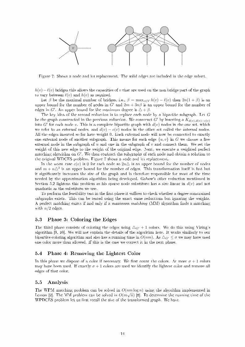
Figure 7: Shows a node and its replacement. The solid edges are included in the edge subset.

h(v)− `(v) bridges this allows the capacities of v that are used on the non bridge part of the graphto vary between `(v) and h(v) as required.

Let β be the maximal number of bridges, i.e., β = maxv∈V h(v) − `(v) then 2n(1 + β) is anupper bound for the number of nodes in G′ and 2m + 3nβ is an upper bound for the number ofedges in G′. An upper bound for the maximum degree is 4+ β.

The key idea of the second reduction is to replace each node by a bipartite subgraph. Let Gbe the graph constructed in the previous reduction. We construct G′ by inserting a Kd(v),d(v)−c(v)

into G′ for each node v. This is a complete bipartite graph with d(v) nodes in the one set, whichwe refer to as external nodes, and d(v) − c(v) nodes in the other set called the internal nodes.All the edges inserted so far have weight 0. Each external node will now be connected to exactlyone external node of another subgraph. This means for each edge {u, v} in G we choose a freeexternal node in the subgraph of u and one in the subgraph of v and connect them. We set theweight of this new edge to the weight of the original edge. Next, we execute a weighted perfectmatching algorithm on G′. We then contract the subgraphs of each node and obtain a solution tothe original WDCES problem. Figure 7 shows a node and its replacement.

In the worst case c(v) is 0 for each node so 2n4 is an upper bound for the number of nodesand m + n42 is an upper bound for the number of edges. This transformation itself is fast butit signi�cantly increases the size of the graph and is therefore responsible for most of the timeneeded by the approximation algorithm being developed. Gabow's other reduction mentioned inSection 5.2 lightens this problem as his sparse node substitute has a size linear in d(v) and notquadratic as the substitute we use.

To perform the feasibility test in the �rst phase it su�ces to check whether a degree constrainedsubgraphs exists. This can be tested using the exact same reductions but ignoring the weights.A perfect matching exists if and only if a maximum matching (MM) algorithm �nds a matchingwith n/2 edges.

5.3 Phase 3: Coloring the Edges

The third phase consists of coloring the edges using 4G′ + 1 colors. We do this using Vizing'salgorithm [9, 10]. We will not explain the details of the algorithm here. It works similarly to ourbipartite coloring algorithm and also has a running time in O(nm). As 4G′ ≤ σ we may have usedone color more than allowed. If this is the case we correct it in the next phase.

5.4 Phase 4: Removing the Lightest Color

In this phase we dispose of a color if necessary. We �rst count the colors. At most σ + 1 colorsmay have been used. If exactly σ + 1 colors are used we identify the lightest color and remove alledges of that color.

5.5 Analysis

The WPM matching problem can be solved in O(nm log n) using the algorithm implemented inLemon [2]. The MM problem can be solved in O(m

√n) [8]. To determine the running time of the

WPDCES problem let us �rst recall the size of the transformed graph. We have

14

n′ = 2n4 ∈ O(n4) and

m′ = m+ n42 ∈ O(n42)

where 4 is the maximum degree of the input graph. We made use of the fact that m ≤ n4/2 forevery graph. The worst case running time is thus

O(n′m′ log n′) = O(n243 log n4) ⊆ O(n5 log n) .

Testing whether a feasible solution exists is faster because we can reduce it to the maximummatching problem, which can be solved faster, namely in time

O(m′√n′) = O(n42

√n4) ⊆ O(n4) .

In the next step, we determine the running time of the weighted degree constrained subgraphalgorithm. The characteristical numbers of the transformed graph are

n′ = ∈ 2n(1 + β) ∈ O(nβ) ,

m′ = 2m+ 3nβ ∈ O(m+ nβ) and

4′ = 4+ β ∈ O(4)

where 4′ is the maximum node degree of the transformed graph and β is maxv∈V h(v)− `(v). Theproblem can thus be solved in time

n′24′3 log n′4′ ∈ O(n2β243 log nβ4) ⊆ O(n245 log n4) ⊆ O(n7 log n)

and the corresponding feasibility test runs in time

n′4′2√n′4′ ∈ O(nσ42

√nβ4) ⊆ O(n44

√n) ⊆ O(n5,5) .

Using the binary search over δ we can solve the �rst and the second phase in time

O((n2β243 log nβ4) + nβ42√nβ4 log t) = O(n2β243 log nβ4)

⊆ O(n5σ2 log n) .

This clearly dominates the third phase, which has a running time of Θ(mn), so this is also theoverall running time. The essence of this section can be summed up in the following theorem.

Theorem 14. The general speed dating problem can be approximated with an absolute performanceguarantee of 1 with respect to the weight criterion and with a relative guarantee of (σ + 1)/σ withrespect to the fairness criterion in time O(n5σ2 log n).

6 Heuristics

The worst-case running time derived in the previous section does not seem satisfactory. We there-fore implemented and evaluated a couple of heuristic algorithms. All of these are greedy algorithmsand have the same top level structure. They associate a key k(e) to each edge e. At each iterationthey insert an edge with maximum key that does not violate any constraints. The algorithms di�eronly in the choice of the key. Algorithm 3 shows this structure in more details. In the followingsubsections we describe the keys used by the di�erent algorithms.

6.1 δ-absolute

Let wmax be the maximum edge weight and d′(v) the node degree of v in the subgraph induced bythe currently selected edge set E′. The key is calculated using the following formula:

k(u, v) = wmax max{0, `(u)− d′(u), `(v)− d′(v)}+ w(u, v)

The �rst term tries to measure how well the δ-criterion would be satis�ed if the edge e wouldbe added to E′. The second does the same for the weight criterion. We multiply the �rst termwith wmax to make sure that the �rst term always dominates the second one unless it is 0.

As adding an edge to E′ changes d′(v) the key values are not constant during the execution ofthe algorithm. All of the keys of the edges adjacent to an edge that is added may decrease by thataction. We use a heap data structure to quickly determine an edge with maximum key value. Therunning time is in O(m4 logm).

15

Algorithm 3 The top level structure of the greedy algorithms considered.

H ← E;E′ ← ∅;For all e ∈ E calculate k(e);while H 6= ∅ do

e← edge with maximum k(e) in H;H ← H\{e};if can add e to E′ without violating the upper capacity constraint then

if can color e without violating the coloring constraint in E′ thenE′ ← E′ ∪ {e};update all k(e) that changed;

end

end

end

6.2 δ-initial

The second algorithm uses a similar formula that does not depend on E′ and therefore provideskeys that are constant over time. This allows us to sort the edges once at the start of the algorithm.The formula is:

k(u, v) = wmax max{`(u), `(v)}+ w(u, v)

The running time is in O(m logm).

6.3 δ-relative

Let c be the least common multiple of all d(v). The third greedy algorithm uses the following keyformula:

k(u, v) = wmaxcmax{ `(v)

d(v),`(u)

d(u)}+ w(u, v)

The multiplication with c makes sure that the �rst term is integer. As it is also a multiple of wmax

it dominates the second term unless it is 0.The ratio `(v)

d(v) describes how many of v's out edges must be included in E′ to achieve a δ value

of 0. If we randomly add edges then we will most likely have problems with nodes were this ratiois near 1. The idea of this greedy algorithm is therefore to add edges to these problematic nodesas early as possible.

The keys are constant over time and therefore it is possible to sort the edges once at the startof the algorithm. The running time is in O(m logm).

16

7 Evaluation

In the previous sections we have developed a number of algorithms and analyzed their theoreticalperformances. In this section we evaluate their running time using an implementation and testdata.

Our �rst solver makes use of the ILP formulation we have given in Section 3.2. It simplyfeeds the input data to an o�-the-shelf ILP solver. We have not tried to tune the ILP solver forthis speci�c problem. In this section we refer to this solver of the speed dating problem as ILP-based solver. Next, we have implemented the algorithm described in Section 4 which solves theheterosexual speed dating problem. We refer to this solver as the bipartite solver as it operatesonly on bipartite graphs. The min cost �ow solver used at the core of this implementation is thenetwork simplex based solver bundled with Lemon [2]. This di�ers from the algorithm that wasused in Section 4.4 to derive a bound for the worst case running time. The author claims thatthe simplex based approach is generally faster even though it has worse theoretical worst caserunning time [1]. We also implemented the approximation algorithm for general graphs describedin Section 5. At its core it makes use of the solver for the general maximal matching problemprovided by Lemon. We will refer to this solver as the general solver. Finally we implemented thethree heuristic greedy algorithms described in Section 6. We refer to them as the absolute solver,the initial solver and the relative solver.

Unfortunately, we do not have any real world data. Therefore, we use random test instances.There is a quite large set of parameters that make up the instances, hence it is impossible to performexhaustive testing. Parameters include the number of people, the number of bad dates, the fairnessconstraints, the date quality distribution and whether we consider homo- or heterosexual dating.We test instances that we suppose could be produced by the original problem statement.

We evaluate how fast our implementations are and how well the produced solution satis�esthe fairness and weight criteria. We perform three test series. The �rst two evaluate the generalperformance of our algorithms. The last one tries to model a real world situation as closely aspossible. As the performances depend on the graph structure we performed each test four timesusing di�erent graphs of the same size to smoothen outliers.

Our tests have been performed on an Intel Core2 Quad Q6600 processor1 with 2GB RAM. Alltests are single threaded, i.e., make only use of a single core. The test were run under Ubuntu 11.1and the compiler was GCC 4.4.1 with an optimization level of -O3.

7.1 Heterosexual Dating

In this experiment we evaluate the performance of our algorithms on bipartite graphs. Because ofthe way we implemented Vizing's algorithm the general solver always manages to color the graphin the third phase using σ colors. It therefore does not have to throw away the lightest color andthus always provides an optimal solution. As we have an optimal and fast solver at our disposal, itmakes no sense to display the performance of the ILP-based or general solvers on any plot exceptthe one showing the running times.

1See http://ark.intel.com/Product.aspx?id=29765 for processor details

17

7.1.1 Varying the Number of People

0.001

0.01

0.1

1

10

100

1000

0 100 200 300 400 500 600 700 800 900 1000

Tim

e (s

)

Node count

ILPGeneralBipartiteRelative

AbsoluteInitial

Figure 8: running times while varying n

In this section we vary the number of people n.For each two women there are three men. Thenumber of bad dates is always set to 2/3 of allpossible dates. There are 3n/5 men and 2n/5women and therefore a total of 6n2/25 pos-sible dates. As 2/3 are bad dates we havem =

⌊2/25 · n2

⌋. Which dates are bad is chosen

at random. For each person we choose ` and hsuch that `(v) ≤ h(v) ≤ 12 randomly along auniform distribution. A dating event with 12dates and 10 min per date will last at least 2hours. We suppose therefore that this producesrealistic values. The date qualities are chosenrandomly from {1, 2, . . . , 100} using a uniformdistribution. We call this graph structure uni-form.

Plot 8 shows the running times of the evaluated algorithms. One can see that the ILP-basedsolver is not even able to handle small instances. The approximation algorithm for general graphsis not quite as slow as our analysis predicted but it is largely outperformed by the remainingalgorithms. What is surprising is that the bipartite algorithm, which produces exact solutions, canrival the speed of the greedy algorithms. The algorithm is by far faster than what our worst casetime analysis predicted. This can be explained to some extent by the fact that we used a di�erentmin cost �ow solver in these tests than in the worst case analysis.

Plot 9 shows the performance of the approximation algorithms with respect to the weightcriterion and the fairness criterion. The weight of the solutions is plotted as di�erence to theoptimal value. The absolute Solver works well whereas the initial solver and the relative solverstruggle a lot. They only �nd solutions that have a δ value of about 3 which is quite large consideringthat solutions with δ = 0 exist. Also the weight criterion is far from being met optimally. Wecan explain these di�erences in performance by the fact that the key of the two bad heuristics areconstant during the execution and the absolute solver may adjust the keys to react to unforeseensituations.

This experiment clearly shows that the bipartite solver is superior in every way to both the ILPas well as the general solver. We will therefore not consider them in the remaining experiments onbipartite graphs.

0

2000

4000

6000

8000

10000

12000

14000

0 100 200 300 400 500 600 700 800 900 1000

Wei

ght d

iffer

ence

Node count

RelativeInitial

Absolute

(a) weight di�erence to optimum

0

1

2

3

4

5

6

7

8

9

0 100 200 300 400 500 600 700 800 900 1000

Fai

rnes

s V

iola

tion

Node count

InitialRelative

AbsoluteOptimum

(b) fairness violation

Figure 9: performance for bipartite uniform graphs while varying n

18

7.1.2 Varying the Number of Dates

In the previous experiment the density of the graph was constant and we varied the size of the graph.To evaluate the e�ect of the density on the performances we perform another experiment, wherewe set n = 1000 and let m vary between 0 and

⌊6/25 · n2

⌋= 240000. All the other parameters are

the same as in the previous experiment.

0

0.5

1

1.5

2

2.5

3

0 50000 100000 150000 200000 250000

Tim

e (s

)

Edge count

AbsoluteInitial

RelativeBipartite

Figure 10: running times while varying m

Figure 10 shows the running times of thefour tested algorithms. The graph density isthe same as in the previous experiment whenm =

⌊2/25 · n2

⌋= 80000. The results observed

at that density are consistent with those of theprevious experiment. It is surprising that forlargem the exact bipartite solver is fastest. Wesuppose that this e�ect is due to the fact thatmany edges have to be discarded by the greedyalgorithms. In our implementation a loop overall colors is needed to discard an edge. Consid-ering that there are only twelve colors this isnot prohibitive but it may explain the runningtimes observed.

Figure 11a shows the performance of thegreedy algorithm with regard to the weight cri-terion. One can see, just as in the previous experiment, that absolute solver outperforms the twoothers. On sparse graphs the algorithms perform rather poorly. Probably there are fewer solutionsthat are close to the optimal one and therefore including a wrong edge in the subset has worserepercussions than when operating on dense graphs.

Figure 11b shows how well the fairness criterion is satis�ed. We can see the same thing asin the previous experiment that the absolute solver is nearly optimal but the two others performpoorly. The peak near the sparse graphs is due to the graph structure as even the optimal fairnessviolation is not near 0.

0

5000

10000

15000

20000

25000

30000

35000

40000

45000

0 50000 100000 150000 200000 250000

Wei

ght d

iffer

ence

Edge count

RelativeInitial

Absolute

(a) weight di�erence to optimum

0

2

4

6

8

10

12

0 50000 100000 150000 200000 250000

Fai

rnes

s V

iola

tion

Edge count

AbsoluteInitial

RelativeOptimum

(b) fairness violation

Figure 11: performance for bipartite uniform graphs while varying m

19

7.1.3 Real World Scenario

Our goal in this experiment is to evaluate how well our algorithms perform in models based on �lledout forms. We suppose each form contains 30 questions and each of them requires the participantto rate something on a scale ranging from 0 to 5. Every person is therefore represented usinga vector vp with 30 elements chosen from the set {0/5, 1/5, . . . , 5/5} randomly along a uniformdistribution. We use the euclidean distance to model the date goodnesses. The maximum distanceof two such vectors is the distance of the vectors (0, 0, 0, . . .) and (1, 1, 1, . . .), which is

√30. Using

this model good dates have a small distance. We however need a large date goodness. To �x thiswe use the following formula to calculate the goodness of a date between the persons p and q:

wp,q =

⌊(

√30

2− |vp − vq|2) · 100

⌋

A date is bad if wp,q ≤ 0. We still suppose that we have three men for every two women. Wetry to make sure that every person gets the maximum number of dates possible. Therefore, we set`(v) = h(v) = 8 for the men and `(v) = h(v) = 12 for the women. A graph with such a structureis called form based.

0.001

0.01

0.1

1

10

100

0 100 200 300 400 500 600 700 800 900 1000

Tim

e (s

)

Node count

GeneralAbsoluteBipartiteRelative

Initial

Figure 12: running times for bipartite form graph

Figure 12 shows the running times of thedi�erent solvers tested. We also tried to eval-uate the ILP-based solver but it was not ca-pable of solving even the smallest instances inreasonable time. The running times are gen-erally slower than in the previous experiments.Surprisingly, the running time of the bipartitesolver is between the running times of the ab-solute solver and the other two greedy solvers.

Figure 13 show the quality of the solutions.They greatly di�er from the results in Section7.1.1. In terms of total weight the absolutesolver still outperforms the two other greedyalgorithms but the di�erence is smaller. Theresults for the fairness violations are very in-teresting. The initial solver performs just asbad as in the previous experiment. The relative solver is a lot better and the absolute solver nolonger manages to achieve the optimum value but is nearly constantly o� by only one.

We suppose that the reason the relative solver performs that well is because it �rst tries tomatch the sparse bridge like parts in the graph. Only once this is done it tries to match the edgesinside the clusters. Each cluster is a rather dense subgraph and therefore it is simpler to �nd amatching with many edges inside it. It is however not as easy to �nd a heavy matching with manyedges and therefore the relative solver performs bad in terms of total matching weight.

0

5000

10000

15000

20000

25000

0 100 200 300 400 500 600 700 800 900 1000

Wei

ght d

iffer

ence

Node count

RelativeInitial

Absolute

(a) weight di�erence to optimum

0

2

4

6

8

10

12

0 100 200 300 400 500 600 700 800 900 1000

Fai

rnes

s V

iola

tion

Node count

InitialRelative

AbsoluteOptimum

(b) fairness violation

Figure 13: performance for bipartite form based graphs

20

7.2 Homosexual Dating

In this section we present similar experiments to the ones in the previous section, however theyexamine general non-bipartite graph structures. As a consequence it is not possible to make use ofthe bipartite solver. We therefore no longer have a solver that can compute optimal solutions forlarge instances. We can therefore not plot the di�erence to the optimal solution as we did in theprevious section but have to resort to plotting the actual values.

7.2.1 Varying the Number of People

This experiment is very similar to the one in Section 7.1.1. There are n(n − 1)/2 possible datesand, to make sure that 2/3 of the dates are bad dates, we set m = bn(n− 1)/6c. The bad dates areagain chosen uniformly at random. Figure 14a shows the running times of the di�erent algorithms.They behave nearly the same as in the bipartite case.

We have also tested how well the weight and the fairness criteria are met. Figure 14b displaysthe result for the total weight. We plot the di�erence to the relative solver. The general solverproduces the best results. The absolute solver is better than the other two greedy algorithms.These two produce solutions that are of the same quality. For the few test cases that the ILPbased solver was able to �nd an optimal solution it found one that has the same quality as thesolution found by the general solver. All solvers �nd nearly always solutions with an optimalfairness violation of zero. We only found a single test instance where the initial solver was o� by1. The plot showing this has been omitted as it would not provide any additional information.

An interesting observation is that these results are di�erent from those in Experiment 7.1.1.Especially, the initial and relative algorithms do not struggle nearly as much as with bipartitegraph structures when considering the fairness violation. It is possible that the good solutions forthe bipartite graph structures make use of characteristic of that structure that these two solvercan not �nd and therefore they are not able to determine the optimal solution.

Consider for a moment the weighted matching problem i.e. each node should be matched once.In graphs with a uniform weight distribution it is in general best to match the edges along aneven cycle in an alternating way. This maximizes the expected total weight sum and providesa perfect matching. As soon as one edge is matched in a way that no such alternating chaincan be constructed anymore one misses out on at least two edges. Greedy algorithms are likelyto do this. As bipartite graphs only contain even cycles these algorithms often fall into this trap.General graphs on the other hand also contain cycles with an odd length. In those cycles no perfectmatching is possible so this matters less. We know that this does not explain this e�ect very well,for example we do not know why the absolute solver can cope with bipartite graphs, however it isthe best attempt at an explanation that we have got.

0.001

0.01

0.1

1

10

100

1000

0 100 200 300 400 500 600 700 800 900 1000

Tim

e (s

)

Node count

ILPGeneral

AbsoluteInitial

Relative

(a) running time

-500

0

500

1000

1500

2000

2500

3000

3500

4000

100 200 300 400 500 600 700 800 900 1000

Wei

ght

Node count

GeneralAbsolute

InitialRelative

(b) weight di�erence to relative

Figure 14: results for uniform graph while varying n

21

7.2.2 Varying the Number of Dates

0

10

20

30

40

50

60

0 1000 2000 3000 4000 5000

Tim

e (s

)

Edge count

General

Figure 15: running times while varying m

In this experiment we will �x n = 100 andvary m between 0 and n(n− 1)/2 = 4950. Theremaining parameters are the same as in theprevious experiment. As the ILP based solveris incapable of producing solutions of this sizewe do not consider it.

Figure 15 shows the running time of thegeneral algorithm. We also measured the timethat the greedy algorithms take but it wasnearly constantly below the resolution of ourtimer. It therefore makes no sense to plot theseresults. Figure 16a shows the achieved weightsof the di�erent algorithms. We plot the di�er-ence to the relative solver. It is interesting thaton dense graphs the di�erence between the gen-eral solver and the greedy solvers diminishes asthe graphs become denser. This e�ect is probably due to the fact that as there are more edgesit is more likely that there are more edges with high weights and as a consequence the greedyalgorithms do not have to use edges with a low weight at the end. The general solver can not makeuse of that many high weight edges as there is a maximum of edges that may be selected and thenumber of these good edges is higher than that limit. Figure 16b shows the values for the fairnessviolation. One should note that all algorithms are capable of �nding optimal solutions most of thetime when one only considers this criterion. Just as in the previous experiment we can observethat the initial and relative algorithms perform a lot better on non bipartite graphs.

-500

0

500

1000

1500

2000

2500

3000

0 1000 2000 3000 4000 5000

Wei

ght

Edge count

GeneralAbsolute

InitialRelative

(a) weight di�erence to relative

0

2

4

6

8

10

12

0 1000 2000 3000 4000 5000

Fai

rnes

s V

iola

tion

Edge count

GeneralAbsolute

InitialRelative

(b) fairness violation

Figure 16: performance on uniform graphs while varying m

22

0

50000

100000

150000

200000

250000

300000

350000

400000

450000

500000

0 100 200 300 400 500 600 700 800 900 1000

Wei

ght

Node count

GeneralAbsolute

InitialRelative

(a) total weight

0

1

2

3

4

5

6

7

8

9

10

0 100 200 300 400 500 600 700 800 900 1000

Fai

rnes

s V

iola

tion

Node count

InitialRelative

AbsoluteGeneral

(b) fairness violation

Figure 17: performance on form graphs

7.2.3 Real World Scenario

0.001

0.01

0.1

1

10

100

1000

0 100 200 300 400 500 600 700 800 900 1000

Tim

e (s

)

Node count

GeneralAbsolute

InitialRelative

Figure 18: running times for form graphs

We also tested the solvers for general graphstructures on form based graphs. Figure 18shows the running times of the di�erent algo-rithms. As we expected the general solver isslow and the rest is fast. Figure 17a showsthe total weights of the solutions produced bythe di�erent solvers and Figure 17b the val-ues for the fairness violation. It is surprisingthat the greedy algorithms struggle a lot morethan with uniform graphs. The initial solveris always worst with a fairness violation signi�-cantly above the optimum. The relative solveris a lot better but its performance varies a lot.The absolute solver is constantly one unit abovethe optimum. The general solver nearly always�nds solutions with an optimal fairness viola-tion of zero.

8 Conclusion

We have formalized the speed dating problem in graph-theoretic terms and as an integer linearprogram. We have shown that heterosexual special case can be solved in polynomial time and thatthe general homosexual problem statement is NP-hard.

We have developed an algorithm that solves the heterosexual special case in at mostO(n2m log(nW ))running time. Our experiments have shown that even for very large events with 1000 people thecomputation time is only slightly above a single second. Let us recall that σ is the number of datingrounds. We described an algorithm that computes an approximate solution for the general case inO(n5σ2 log n) running time. The weight of the solution found by our approximation algorithm isat least σ/(σ + 1) times the total weight of an optimal solution and the fairness violation is o� byat most one unit. Empirical results show that our algorithm nearly always �nds a solution withan optimal fairness violation and that the running time is acceptable with 5 minutes for a mediumsized event of 200 people. The algorithm will perform better the more dating rounds the eventhas, as σ/(σ + 1) tends to 1 for σ →∞.

It turned out that the matching aspect can be solved in polynomial time but requires a lotof implementation work. We were only able to solve the scheduling subproblem e�ciently for theheterosexual special case. The implementation work was however a lot easier. In the homosexualcase the two subproblems can not be treated separately which complicates the problem of �ndingan optimal solution considerably. If one treats them separately then it is possible that schedulingproblem becomes unsolvable.

23

We also investigated a number of di�erent greedy approaches. It turned out that their perfor-mance heavily depends on the graph structure. Interestingly, di�erent approaches perform vastlydi�erent on di�erent graph structures. Our tests show that we have found one approach thatprovides solutions of decent quality even for large homosexual events. The running time is slightlybelow 10 seconds for 1000 people.

Starting Points for Follow-up Work

Our approximation algorithm does not make use of the best reductions known for solving theweighted degree constrained edge subset subproblem. It is possible to use the other reductiondescribed by Harold [6]. This will certainly speed up the algorithm and lower the worst case runningtime but it will signi�cantly increase the implementation work. Further our Phase 1 algorithm isoptimized for a uniformly distributed fairness violation. However in most cases relevant to theoriginal problem this violation is zero. Making use of this knowledge one can easily achieve a speedup. Instead of determining the minimal violation using a binary search, one can just guess that itis zero and one would almost always be lucky. It would certainly be interesting to investigate towhat extent our algorithm can still be optimized.

Our tests have revealed that the performance of the initial and relative greedy algorithmspresented here largely depends on the graph structures on which they are run. We have notinvestigated this e�ect. An interesting question is which are the exact graph features that triggerthis behavior. One could try to derive performance guarantees for these graph classes. Further,it would be interesting to see what the worst case performance for the absolute greedy algorithmactually is.

We have concentrated on determining the actual date rounds and have deliberately ignoreda number of aspects of the original problem. For example we have not investigated what theoptimal order of the rounds is. One could gather additional requirements imposed by the realworld situation and try to formalize these as algorithmic problem. Once this is done an obviousquestion is how to solve these e�ciently.

Acknowledgment

I want to thank my advisors Bastian Katz and Ignaz Rutter for supporting me in a multitude ofways and for having always time and patience for questions and interesting discussions.

References

[1] LEMON minimum cost �ow documentation. http://lemon.cs.elte.hu/pub/doc/1.2/

a00527.html.

[2] Library for e�cient modeling and optimization in networks (LEMON). http://lemon.cs.

elte.hu/.

[3] Thomas L. ; Orlin James B. Ahuja, Ravindra K. ; Magnanti. Network �ows : theory, algo-rithms, and applications. Prentice Hall, Upper Saddle River, NJ [u.a.], 1993.

[4] Richard Cole and John Hopcroft. On edge coloring bipartite graphs. SIAM Journal onComputing, 11(3):540�546, 1982.

[5] Reinhard Diestel. Graph Theory (Graduate Texts in Mathematics). Springer, Berlin, Germany,August 2005.

[6] H. N. Gabow. An e�cient reduction technique for degree-constrained subgraph and bidirectednetwork �ow problems. In STOC '83: Proceedings of the �fteenth annual ACM symposium onTheory of computing, pages 448�456, New York, NY, USA, 1983. ACM.

[7] Ian Holyer. The NP-completeness of edge-coloring. SIAM Journal on Computing, 10(4):718�720, 1981.

[8] S. Micali and V.V. Vazitani. An O(V 1/2E) algorithm for �nding maximum matching in generalgraphs. In Proceedings of the 21st Annual IEEE Symposium on Foundations of ComputerScience, pages 17�27, 1980.

24

[9] J. Misra and David Gries. A constructive proof of vizing's theorem. Inf. Process. Lett.,41(3):131�133, 1992.

[10] Michele Zito. http://www.csc.liv.ac.uk/~michele/TEACHING/COMP309/2003/vizing.

pdf. 2003.

25