speeded up robust features (surf) · surf: speeded up robust features • speed-up computations by...

Speeded Up Robust Features (SURF)

Harris corner detector algorithm-Compute magnitude of the gradient everywhere in x

and y directions - Compute - Convolve these three images with a Gaussian window,

w. Find M for each pixel,

- Compute detector response, R at each pixel.

- find local maxima above some threshold on R. Compute nonmax suppression.

I2x , I2

y , IxIy

Ix, Iy

M = ∑ w(x, y)[I2x IxIy

IxIy I2y ]

R = det(M) − k(trace(M))2

Applications of SIFT

• Object recognition • Object categorization • Location recognition • Robot localization • Image retrieval • Image panoramas

Object RecognitionObject Models

Object Categorization

Location recognition

Robot Localization

Map continuously built over time

SIFT Computation – Steps

(1) Scale-space extrema detection – Extract scale and rotation invariant interest points (i.e., keypoints).

(2) Keypoint localization – Determine location and scale for each interest point. – Eliminate “weak” keypoints

(3) Orientation assignment – Assign one or more orientations to each keypoint.

(4) Keypoint descriptor – Use local image gradients at the selected scale.

D. Lowe, “Distinctive Image Features from Scale-Invariant Keypoints”, International Journal of Computer Vision, 60(2):91-110, 2004.

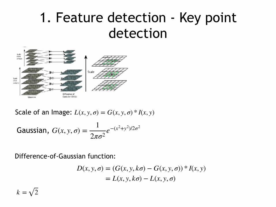
1. Feature detection - Key point detection

Scale of an Image: L(x, y, σ) = G(x, y, σ) * I(x, y)

Gaussian, G(x, y, σ) =1

2πσ2e−(x2+y2)/2σ2

Difference-of-Gaussian function:

D(x, y, σ) = (G(x, y, kσ) − G(x, y, σ)) * I(x, y)= L(x, y, kσ) − L(x, y, σ)

k = 2

1. Key point localization

• Detailed fit using data surrounding the keypoint to Localize extrema by fitting a quadratic, to nearby data for location, scale and ratio of principal curvatures

1) Sub-pixel/sub-scale interpolation using Taylor expansion

D( x ) = D +∂DT

∂ xx +

12

x T ∂2D∂ x 2

x x = (x, y, σ)T;

Location of the extrema, x = −∂2D∂x2

−1 ∂D∂x

by taking a derivative and setting it to zero

1. Key point localization

1) Sub-pixel/sub-scale interpolation using Taylor expansion

D( x ) = D +∂DT

∂ xx +

12

x T ∂2D∂ x 2

x x = (x, y, σ)T;

Location of the extrema, x = −∂2D∂x2

−1 ∂D∂x

∂D∂x

=

∂D∂x∂D∂y∂D∂σ

=

D(x + 1,y, σ) − D(x − 1,y, σ)2

D(x, y + 1,σ) − D(x, y − 1,σ)2

D(x, y, σ + 1) − D(x, y, σ − 1)2

D( x) = D +12

∂D∂x

x Discard |D( x) | < 0.03key points with low contrast

1. Key point localization - Eliminating edge response

1) Principal curvatures can be computed from a 2 x 2 Hessian matrix

H = [Dxx Dxy

Dxy Dyy]

∂D∂x

=


=

D(x + 1,y, σ) − D(x − 1,y, σ)2

D(x, y + 1,σ) − D(x, y − 1,σ)2

D(x, y, σ + 1) − D(x, y, σ − 1)2

1. Key point localization - Eliminating edge response

1) Principal curvatures can be computed from a 2 x 2 Hessian matrix

H = [Dxx Dxy

Dxy Dyy]∂D∂x

=


=

D(x + 1,y, σ) − D(x − 1,y, σ)2

D(x, y + 1,σ) − D(x, y − 1,σ)2

D(x, y, σ + 1) − D(x, y, σ − 1)2

Dxy =D(x + 1,y + 1,σ) − D(x − 1,y + 1,σ)

2 − D(x + 1,y − 1,σ) − D(x − 1,y − 1,σ)2

2

1. Feature detection - Keypoint localization

• Discard low-contrast/edge points 1) Low contrast: discard keypoints with

threshold < 0.03 2) Edge points: high contrast in one direction, low

in the other ! compute principal curvatures from eigenvalues of 2x2 Hessian matrix, and limit ratio

r =αβ

r= 10

2. Orientation Assignment

– Assign canonical orientation at peak of smoothed histogram

• Assign orientation to keypoints

m(x, y) = (L(x + 1,y) − L(x − 1,y))2 + (L(x, y + 1) − L(x, y − 1))2

Gradient magnitude,

Orientation,

θ(x, y) = tan−1( L(x, y + 1) − L(x, y − 1)L(x + 1,y) − L(x − 1,y) )

2. Orientation Assignment

– Create histogram of local gradient directions computed at selected scale

• Assign orientation to keypoints

Orientation histogram has 36 bins each covering 10 degrees

Peaks in the orientation histogram correspond to dominant directions of local gradients.

Any other local peak, within 80% of the highest peak is also used to create a key point with that orientation.

There may be multiple key points with same location and scale but different orientation.

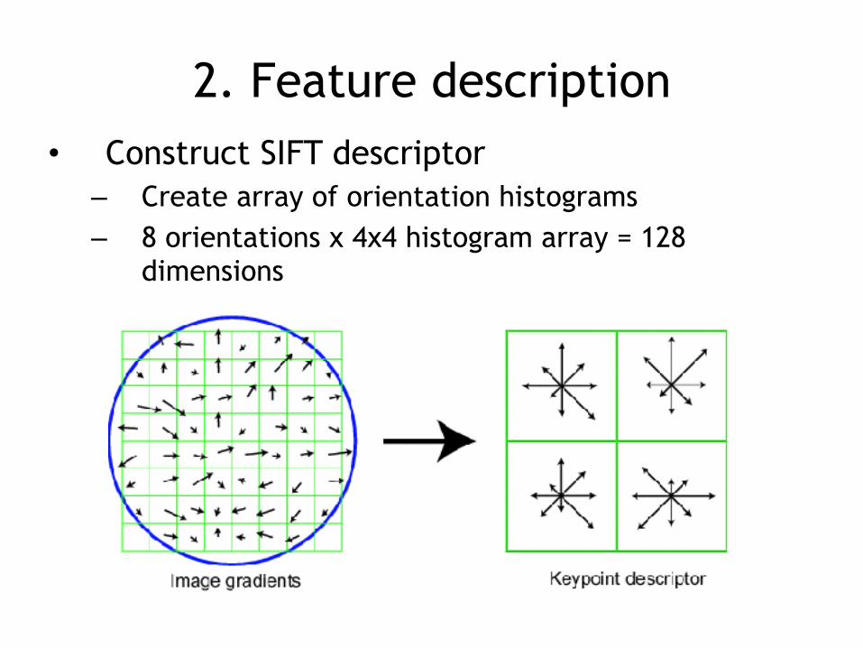
2. Feature description• Construct SIFT descriptor – Create array of orientation histograms – 8 orientations x 4x4 histogram array = 128

dimensions

2. Feature description• Advantage over simple correlation – less sensitive to illumination change – robust to deformation, viewpoint change

4. Keypoint Descriptor (cont’d)

16 histograms x 8 orientations = 128 features

1. Take a 16 x16 window around detected interest point.

2. Divide into a 4x4 grid of cells.

3. Compute histogram in each cell.

(8 bins)

Matching SIFT features

• Given a feature in I1, how to find the best match in I2? 1. Define distance function that compares two descriptors. 2. Test all the features in I2, find the one with min distance.

I1 I2

Matching SIFT features (cont’d)•

I1 I2

f1 f2

Matching SIFT features (cont’d)

• Accept a match if SSD(f1,f2) < t • How do we choose t?

Matching SIFT features (cont’d)• A better distance measure is the following:

– SSD(f1, f2) / SSD(f1, f2’)

• f2 is best SSD match to f1 in I2

• f2’ is 2nd best SSD match to f1 in I2

I1 I2

f1 f2f2'

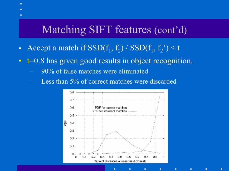
Matching SIFT features (cont’d)• Accept a match if SSD(f1, f2) / SSD(f1, f2’) < t • t=0.8 has given good results in object recognition.

– 90% of false matches were eliminated. – Less than 5% of correct matches were discarded

Variations of SIFT features

• PCA-SIFT

• SURF

• GLOH

SURF: Speeded Up Robust Features

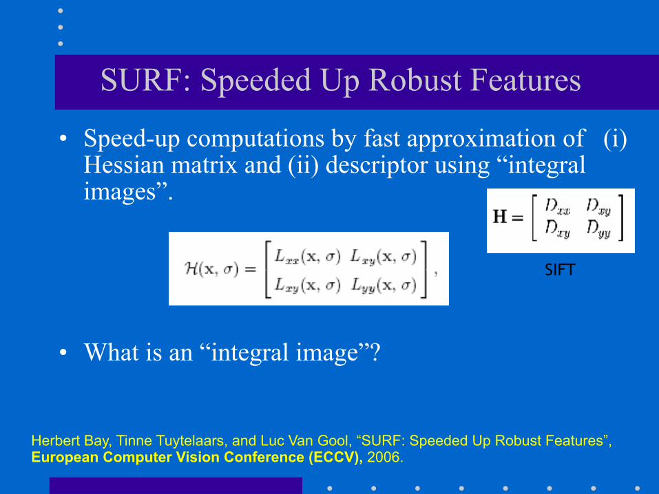
• Speed-up computations by fast approximation of (i) Hessian matrix and (ii) descriptor using “integral images”.

• What is an “integral image”?

Herbert Bay, Tinne Tuytelaars, and Luc Van Gool, “SURF: Speeded Up Robust Features”, European Computer Vision Conference (ECCV), 2006.

SIFT

Integral Image

• The integral image IΣ(x,y) of an image I(x, y) represents the sum of all pixels in I(x,y) of a rectangular region formed by (0,0) and (x,y).

• . Using integral images, it takes only four array references to calculate the sum of pixels over a rectangular region of any size.

0 0( , ) ( , )

j yi x

i jI x y I i j

≤≤

Σ= =

=∑∑

SURF: Speeded Up Robust Features (cont’d)

• Approximate Lxx, Lyy, and Lxy using box filters.

• Can be computed very fast using integral images!

(box filters shown are 9 x 9 – good approximations for a Gaussian with σ=1.2)

derivative approximation approximationderivative


• In SIFT, images are repeatedly smoothed with a Gaussian and subsequently sub-sampled in order to achieve a higher level of the pyramid.


• Alternatively, we can use filters of larger size on the original image.

• Due to using integral images, filters of any size can be applied at exactly the same speed!

(see Tuytelaars’ paper for details)


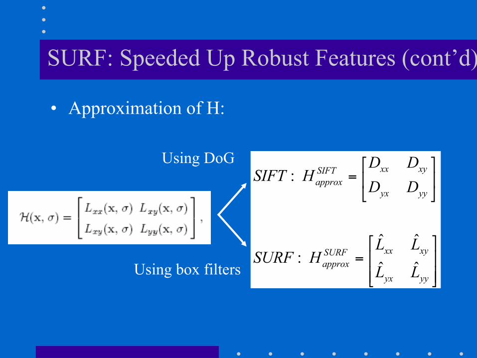
• Approximation of H:

:

ˆ ˆ: ˆ ˆ

xx xySIFTapprox

yx yy

xx xySURFapprox

yx yy

D DSIFT H

D D

L LSURF H

L L

⎡ ⎤= ⎢ ⎥⎣ ⎦

⎡ ⎤= ⎢ ⎥⎢ ⎥⎣ ⎦

Using DoG

Using box filters


• Instead of using a different measure for selecting the location and scale of interest points (e.g., Hessian and DOG in SIFT), SURF uses the determinant of to find both.

• Determinant elements must be weighted to obtain a good approximation:

SURFapproxH

2ˆ ˆ ˆdet( ) (0.9 )SURFapprox xx yy xyH L L L= −

Harris corners


• Once interest points have been localized both in space and scale, the next steps are: (1) Orientation assignment (2) Keypoint descriptor


• Orientation assignment Circular neighborhood of

radius 6σ around the interest point (σ = the scale at which the point was detected)

Haar wavelets (responses weighted with Gaussian) Side length = 4σ

x response y response

Can be computed very fast using integral images!

600 angle

( , )dx dy∑ ∑


• Sum the response over each sub-region for dx and dy separately.

• To bring in information about the polarity of the intensity changes, extract the sum of absolute value of the responses too.

Feature vector size: 4 x 16 = 64

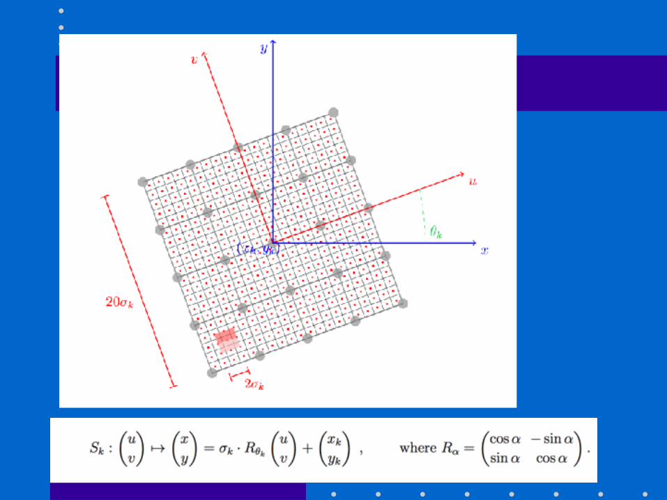
• Keypoint descriptor (square region of size 20σ)

4 x 4 grid


• SURF-128 – The sum of dx and

|dx| are computed separately for points where dy < 0 and dy >0

– Similarly for the sum of dy and |dy|

– More discriminatory!

SURF: Speeded Up Robust Features

• Has been reported to be 3 times faster than SIFT.

• Less robust to illumination and viewpoint changes compared to SIFT.

K. Mikolajczyk and C. Schmid,"A Performance Evaluation of Local Descriptors", IEEE Transactions on Pattern Analysis and Machine Intelligence, vol. 27, no. 10, pp. 1615-1630, 2005.

OpenCV packages

• FindHomography • FlannBasedMatcher FLANN stands for Fast Library

for Approximate Nearest Neighbors. It contains a collection of algorithms optimized for fast nearest neighbor search in large datasets and for high dimensional features.

o Uses k-d trees

speeded up robust features (surf) · surf: speeded up robust features • speed-up computations by...

Documents