spending needs, tax revenue capacity and the business ... · recent years have seen big changes to...
TRANSCRIPT
Spending needs, tax revenue capacity and the business rates retention scheme
Living Standards, Poverty and Inequality in the UK: 2016
Neil Amin-SmithDavid Phillips Polly Simpson

Spending needs, tax revenue capacity and the business rates retention scheme
Neil Amin-Smith David Phillips Polly Simpson
Copy-edited by Judith Payne
The Institute for Fiscal Studies

Published by
The Institute for Fiscal Studies
7 Ridgmount Street London WC1E 7AE
Tel: +44 (0) 20-7291 4800 Fax: +44 (0) 20-7323 4780 Email: [email protected] Website: http://www.ifs.org.uk
© The Institute for Fiscal Studies, February 2018
ISBN 978-1-911102-81-6

Preface The report was funded by IFS’s Local Government Finance and Devolution consortium. The main consortium supporters are:
the Economic and Social Research Council (ESRC); PwC; Capita; the Chartered Institute of Public Finance and Accountancy (CIPFA).
Additional consortium supporters include:
the Municipal Journal; the Society of County Treasurers; a range of councils from across England.
The authors would like to thank members of the consortium group and Paul Johnson for providing helpful comments on earlier drafts of this work. Any errors and all views expressed are those of the authors alone.

Contents Executive summary 5 1. Introduction 8 2. Assessed spending needs 9
2.1 How do we estimate spending needs? 9 2.2 How do spending needs per person vary around the country? 11 2.3 What drives spending needs? 13 2.4 How did spending needs change over time? 15 2.5 How do changes in spending needs relate to changes in local
characteristics? 17 3. Tax revenue capacity 19
3.1 How do we measure tax revenue capacity? 19 3.2 How does tax revenue capacity vary around England? 20 3.3 How is tax revenue capacity related to local characteristics? 23 3.4 How has tax revenue capacity changed over time? 25 3.5 How do changes in tax revenue capacity relate to changes in local
characteristics? 27 4. Analysis of 100% rates retention 29
4.1 Revenue capacity and spending needs 29 4.2 Simulating funding under 100% business rates retention 31
5. Conclusion 41 Appendix A 44 References 47 Data references 48
Executive summary
© Institute for Fiscal Studies 5
Executive summary Recent years have seen big changes to the local government finance system. These include the ending of annual spending needs assessments and the introduction of the business rates retention scheme (BRRS) in 2013–14. This scheme has allowed councils to retain up to 50% of the real-terms growth in local business rates revenues and bear up to 50% of any real-terms falls. The government has announced plans to increase this share to 75% by 2020–21 and continues to expand a series of pilots of 100% retention in certain (volunteer) areas. The aim of these reforms is to provide stronger financial incentives for councils to boost local economies and tackle the underlying drivers of spending need. However, the flip side of these stronger incentives is a greater potential for councils’ revenues to diverge from their spending needs.
How big could these divergences be? Since we do not know how revenues and needs will evolve in future, in this report we look at how local tax revenue-raising capacity and assessed spending needs varied and changed between 2006–07 and 2013–14, the most recent years for which data on both are available. We then model how the relative levels of funding for different councils could have evolved under different versions of 100% business rates retention if such systems had been in place during this period. This allows us to get a sense of the potential scale of the divergences between councils’ revenues and their assessed needs that could open up over the medium term, and how this is affected by the design of the BRRS.
Assessed spending needs per person vary significantly across councils
95% of the variation in assessed relative spending needs across council areas in 2013–14 can be explained simply by differences in population size. However, there were significant differences in assessed spending needs per person: one-in-ten council areas were assessed to need 15% less than the national average spending per person, while another one-in-ten were assessed to need 25% more than the average.
In general, needs were assessed to be higher for councils in London and northern regions of England than in southern regions and the East of England. Assessed needs per person were also higher in more urban council areas than in more suburban or rural areas. In large part, this reflects that the existing needs assessment places a significant weight on levels of socio-economic deprivation: 60% of the variation in assessed needs per person can be accounted for by variation in councils’ average scores on the Index of Multiple Deprivation.
Assessed spending needs converged a little between 2006–07 and 2013–14
Those areas with initially higher assessed needs per person tended to see their assessed relative needs fall a little, whilst those with initially lower needs tended to see their assessed relative needs increase a little. The tenth of councils with the highest assessed spending need per person in 2006–07 saw their relative needs fall by on average 7.3% by 2013–14 (although their absolute needs may still have risen). On the other hand the tenth with the lowest initial needs saw their relative needs rise by 3.7%.
Spending needs, tax revenue capacity and the business rates retention scheme
6 © Institute for Fiscal Studies
This can be explained, in part, by the fact that those areas with high levels of assessed needs in 2006–07 saw a fall in their relative levels of deprivation compared with the rest of the country. Similarly, they saw slower growth in the share of their population that was elderly than the rest of the country. This latter trend is likely to continue, which could lead to a further narrowing of the gap in spending needs per person between high- and low-needs areas.
Changes in business rates revenue-raising capacity are uncorrelated with population or economic growth
Councils’ capacity to raise revenue from council tax and business rates varies significantly around the country. And in general, revenue-raising capacity per person was negatively correlated with assessed spending needs per person in 2013–14. This means that without large-scale redistribution of tax revenues between councils, their ability to fund services would vary greatly.
Changes in population size can explain 39% of the variation in changes in councils’ ability to raise council tax revenues between 2006–07 and 2015–16. But changes in population can explain only 3% of the variation in changes in capacity to raise revenues from business rates during the same period. This suggests that increasing the extent to which councils rely on business rates for their revenues will increase the potential for large changes in their revenues per person over time.
The BRRS strips out the impact of revaluation of business properties on the revenues councils actually retain from the scheme. This means the incentives provided by the BRRS relate to changes in the quantity of floor space and its use (e.g. as cheaper industrial or more expensive office or retail property), rather than to changes in underlying property values.
There was also no correlation between changes in councils’ business rates tax bases and changes in local gross value added (GVA) and employment during the period 2010–11 to 2015–16: a period during which there was no revaluation, so changes in tax bases reflect changes in floor space and usage (as well as business rates appeals). In other words, at least in the recent past, there has not been a clear link between the measure of business rates revenues councils are incentivised to grow and broader local economic growth.
By contrast, there was a modest positive correlation between increases in property values at the 2017 revaluation and these measures of economic activity since the previous revaluation in 2010. This suggests that allowing councils to retain the gains or losses in revenues from revaluations could provide incentives more closely aligned to broader economic growth. However, there is also a risk that retention of gains/losses resulting from revaluation could weaken the incentive councils have for promoting property development if an increase in the supply of properties pushes down values.
Significant funding divergences could open up under a 100% BRRS, but their scale would depend on the precise design of the scheme
To get a sense of the scale of divergences that could open up between councils’ tax revenue capacities and their relative spending needs under 100% retention we estimate
Executive summary
© Institute for Fiscal Studies 7
the impact such a scheme could have had if had been in place between 2006–07 and 2013–14. We do this on the basis of each council setting council tax at the national average rate. This allows us to focus on changes in the distribution of funding across councils that would have been caused by changes in tax bases, rather than different choices over council tax rates.
We need a measure of the divergences between councils’ relative spending needs and the share of overall funding that they would receive under our modelled 100% rates retention schemes. The measure we choose is the ratio of a council’s share of national revenues from council tax and business rates to its share of national assessed spending needs. A figure of 100% indicates that its share of revenues matches its share of assessed needs. Figures higher than 100% indicate a share of revenues that is higher than a council’s share of needs, and vice versa.
We begin by simulating the impact of a 100% rates retention system that is based on scaling up the shares allocated to different councils under 50% retention. We find that even after a full initial equalisation of revenues and needs in 2006–07, by 2013–14, one-in-ten councils would have a revenue-to-relative-needs ratio of less than 92.5%. That is, their share of revenues would be at least 7.5% lower than their share of assessed spending needs. A further one-in-ten councils would have had a ratio of greater than 116%. These sorts of differences in relative funding ratios could lead to differences in the quality and quantity of services different councils are able to offer.
A safety net would have limited the largest shortfalls in funding. For example, a safety net set at the level proposed by the government in its consultation on 100% rates retention would have seen the council in the worst position receiving a share of revenues equal to 87% of its share of needs, as opposed to 61% in the absence of a safety net. However, safety-net payments would blunt the financial incentive of councils in receipt of them to grow their business rates revenues: safety-net payments are reduced one-for-one as rates revenues increase.
In areas with two-tier local government, where business rates revenues are shared between counties and shire districts, the extent of divergence in funding would depend crucially on the share of business rates allocated to each council type (the ‘tier share’).
Under 50% retention, districts retain 80% of the local share and counties 18%; our baseline scenario under 100% retention maintains this ratio. We find that this would mean significant divergences in funding between districts – by 2013–14, individual districts’ shares of national revenue capacity would have ranged from 61% to 166% of their shares of national spending need.
Allocating a larger initial share of business rates to counties and a smaller initial share to districts would reduce such divergences between districts without substantially increasing divergences between counties. This is because counties have larger and more diverse tax bases (including much higher revenues from council tax). It would also protect counties from seeing their retained revenues fall relative to other councils if, as has historically been the case, business rates revenues grow in real terms. Of course, changing tier shares in this way would mean a shift in the financial incentive to grow business rates revenues from districts to counties as well.

Spending needs, tax revenue capacity and the business rates retention scheme
8 © Institute for Fiscal Studies
1. Introduction For over 50 years, central government grants were provided to English councils with the aim of compensating for differences in the size of local tax bases and spending needs. And from 1990 onwards, business rates revenues were pooled at a national level and redistributed to councils as part of this grant funding.
However, recent years have seen a move away from this system. Beginning in 2013–14, the business rates retention scheme (BRRS) has allowed councils to retain up to 50% of the real-terms growth in local business rates revenues – and bear up to 50% of any real-terms falls in local revenues. 2013–14 was also the last year for which the local spending needs assessments used to allocate grant funding were updated. Together these changes mean councils have stronger financial incentives to grow local tax bases and reduce local spending needs, but also a greater risk of short-term volatility and longer-term divergences between funding and spending needs opening up.
Prior to the June 2017 general election, the Ministry of Housing, Communities and Local Government (MHCLG)1 was planning for councils to bear 100% of the real-terms change in business rates revenues in their areas from April 2019.2 However, the legislation required to take forward key parts of this plan was not resurrected following the June 2017 election, and in December 2017 a new plan was announced: 75% business rates retention from April 2020.3 The government is continuing to pilot 100% retention in parts of England though, suggesting it remains interested in this policy. Either way, increasing the share of changes in business rates revenues retained by councils – whether to 75% or 100% – will further increase the financial incentives councils have to grow these revenues, but also potentially increase the risk of funding divergences between councils.
The extent to which the funding available to different councils will diverge over time under the BRRS will depend both on what happens to local revenues and spending needs and on the precise details of the scheme put in place. This report examines both issues utilising historic revenues data and spending needs assessment formulae data from MHCLG. This allows us to get a sense of how large funding divergences could become in future.
The report proceeds as follows. Chapter 2 looks at how assessed relative spending needs varied around England as of 2013–14, the most recent year for which data are available, and how these patterns had changed over the preceding seven years. Chapter 3 investigates how council tax and business rates revenue-raising potential has varied and changed in recent years, focusing in particular on how this relates to changes in local economic activity. Chapter 4 then examines how changes in assessed spending needs and tax revenue potential correlated during the period 2006–07 to 2013–14. It also examines the extent to which revenues could have diverged from assessed needs over that period if, after an initial equalisation, councils bore 100% of the real-terms changes in their tax revenues and their relative spending needs. Chapter 5 concludes, drawing out the implications of our analysis for future business rates retention policy.
1 Prior to 8 January 2018, MHCLG was the Department for Communities and Local Government (DCLG). In this
report, we refer to the department as MHCLG but the source for reports and data from prior to 8 January 2018 is listed as DCLG.
2 Department for Communities and Local Government, 2017a. 3 Department for Communities and Local Government, 2017b.

Assessed spending needs
© Institute for Fiscal Studies 9
2. Assessed spending needs English councils are responsible for a wide range of public services, including waste collection and disposal, libraries and leisure centres, housing, maintenance of local roads, support for local buses, and – most significantly – social services for children and adults alike.4 The cost of delivering these services to a particular standard can vary across the country, due to input cost differences (such as wages and building space) and to differences in the level of service provision required to meet that standard. For example, an area with more roads will require more spending to make sure that those roads are adequately maintained. Similarly, an area with a larger number of low-income old people with health problems will require more spending on adult social services to meet residents’ care needs. These cost differences are often referred to as differences in local spending needs.
In this chapter, we examine how spending needs, as assessed by MHCLG, varied around England in 2013–14, the last year for which we have an official assessment. We also examine how relative assessed spending needs changed over the preceding seven years. Variations in both the level of, and changes in, spending needs have implications for the potential impact of business rates retention on the funding of different councils.
2.1 How do we estimate spending needs?
Defining and measuring the spending needs of different councils is difficult. A given council’s spending needs will be a function of: (1) the range and quality of services expected of it; and (2) the local geographic and socio-economic characteristics that will affect the cost of providing this service package. In this analysis, we abstract from the first of these issues, focusing on how relative spending needs differ across councils as a result of differences in their characteristics.
To do this, we make use of the official assessment of relative spending needs by MHCLG that was in operation between 2006–07 and 2013–14. A number of assessment methodologies were in use during this period. For a few small service areas – such as coastal protection – the assessment was based on past expenditure for the council in question. However, for most service areas, the assessment was based on the historical relationship between spending and the geographic and socio-economic characteristics of local areas. To do this, formulae linking spending and these characteristics were estimated, either at the council level or, where such data were available, at the ward level. These formulae, as well as the most up-to-date information on each council’s characteristics, were then used to calculate an assessed relative spending need for each council every year during the period. Box 1.1 provides further technical detail.
4 English councils have also traditionally had responsibility for managing and funding the state school system.
However, from 2006–07 this was funded largely from a separate grant outside the general local government finance system (the Dedicated Schools Grant), and the academies and free schools programmes mean a growing number of schools (and associated funding) have been moving out of the local government system entirely.

Spending needs, tax revenue capacity and the business rates retention scheme
10 © Institute for Fiscal Studies
Box 2.1. MHCLG’s spending needs assessment (2006–07 to 2013–14)
Rather than one formula assessing the overall spending needs of a council, there are separate formulae for different service areas, termed service blocks, and sometimes within them sub-blocks. For example, ‘children’s services’ is a service block, divided into three sub-blocks with their own formulae: ‘youth and community’, ‘local authority central education functions’ and ‘children’s social care’. On the other hand, ‘highways maintenance’ is a service block without any sub-blocks.
Most formulae work in broadly the same way. To start with, each council is allocated an initial level of need based on the number of relevant units it contains. A unit is normally a person who lives in that council area (e.g. a child in the case of children’s services), but can be something else (e.g. a kilometre of road in the case of highways maintenance). In addition to this, there are per-unit top-ups reflecting drivers of spending need over and above the number of units. For example, in 2013–14, the formula for the highways maintenance block set spending need per kilometre of roads as follows:
Spending need per km
= Basic amount per km
+ Usage top-up based on ‘traffic flow’ and ‘daytime population per km’
+ Winter top-up based on ‘days with snow lying’ and ‘predicted gritting days’
The basic amount and any top-ups are then added together and multiplied by the number of units (e.g. children, road kilometre) in the council area. So in our example:
Initial highways maintenance need = Km of roads × Spending need per km
Once the initial need has been calculated, the scores for sub-blocks are summed and an area cost adjustment (ACA) is then applied to each service block as a whole. ACAs adjust for differences in both labour costs and business rates bills between councils and are applied to each service block depending on the relevant proportion of expenditure in that block that goes on labour and business rates. In our example:
Final highways maintenance need = Initial highways maintenance need × ACA
Finally, each council’s overall assessed need is calculated by summing scores across blocks according to weights set by MHCLG.
Such an approach to estimating needs is not without its problems. First, the characteristics included in the formulae may not capture the full variation in needs. Second, any estimated relationship of this sort is subject to statistical margins of error. Third is that historical spending levels – which are used in the formulae estimating needs – may not only reflect differences in needs. They could also reflect differences in the efficiency with which different councils deliver services, in the preferences of local people and politicians for different services, and in the historical availability of funding in different areas. If these
Assessed spending needs
© Institute for Fiscal Studies 11
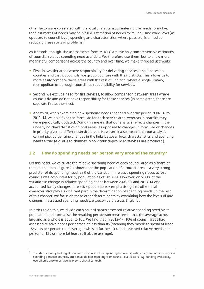
other factors are correlated with the local characteristics entering the needs formulae, then estimates of needs may be biased. Estimation of needs formulae using ward-level (as opposed to council-level) spending and characteristics, where possible, is aimed at reducing these sorts of problems.5
As it stands, though, the assessments from MHCLG are the only comprehensive estimates of councils’ relative spending need available. We therefore use them, but to allow more meaningful comparisons across the country and over time, we make three adjustments:
First, in two-tier areas where responsibility for delivering services is split between counties and district councils, we group counties with their districts. This allows us to more easily compare these areas with the rest of England, where a single unitary, metropolitan or borough council has responsibility for services.
Second, we exclude need for fire services, to allow comparison between areas where councils do and do not have responsibility for these services (in some areas, there are separate fire authorities).
And third, when examining how spending needs changed over the period 2006–07 to 2013–14, we hold fixed the formulae for each service area, whereas in practice they were periodically updated. Doing this means that our analysis reflects changes in the underlying characteristics of local areas, as opposed to changes in formulae or changes in priority given to different service areas. However, it also means that our analysis cannot pick up genuine changes in the links between local characteristics and spending needs either (e.g. due to changes in how council-provided services are produced).
2.2 How do spending needs per person vary around the country?
On this basis, we calculate the relative spending need of each council area as a share of the national total. Figure 2.1 shows that the population of a council area is a very strong predictor of its spending need: 95% of the variation in relative spending needs across councils was accounted for by population as of 2013–14. However, only 39% of the variation in change in relative spending needs between 2006–07 and 2013–14 was accounted for by changes in relative populations – emphasising that other local characteristics play a significant part in the determination of spending needs. In the rest of this chapter, we focus on these other determinants by examining how the levels of and changes in assessed spending needs per person vary across England.
In order to do this, we divide each council area’s assessed relative spending need by its population and normalise the resulting per-person measure so that the average across England as a whole is equal to 100. We find that in 2013–14, 10% of council areas had assessed relative needs per person of less than 85 (meaning they ‘need’ to spend at least 15% less per person than average) whilst a further 10% had assessed relative needs per person of 125 or more (at least 25% above average).
5 The idea is that by looking at how councils allocate their spending between wards rather than at differences in
spending between councils, one can avoid bias resulting from council-level factors (e.g. funding availability, overall efficiency of service delivery, political control).

Spending needs, tax revenue capacity and the business rates retention scheme
12 © Institute for Fiscal Studies
Figure 2.1. Correlation between share of assessed spending needs and population, 2013–14
Note: Excludes Isles of Scilly.
Source: Authors’ calculations using Department for Communities and Local Government (2013a) and Office for National Statistics (2015a).
Table 2.1. Average spending needs per person by region and council type, 2013–14
Spending needs per person
London 115
North East 109
North West 105
West Midlands 103
Yorkshire and the Humber 100
East Midlands 95
South West 95
East of England 92
South East 88
London boroughs 115
Metropolitan districts 109
Unitary authorities 98
Two-tier areas 90
England 100
Note: The table shows a relative measure of spending needs, with mean = 100.
Source: As for Figure 2.1.
0.0%
0.5%
1.0%
1.5%
2.0%
2.5%
3.0%
0.0% 0.5% 1.0% 1.5% 2.0% 2.5% 3.0%
Shar
e of
nat
iona
l spe
ndin
g ne
ed
Share of national population
Assessed spending needs
© Institute for Fiscal Studies 13
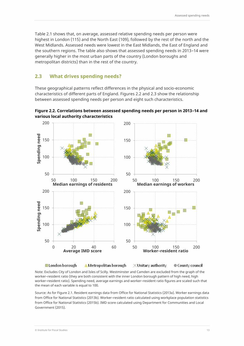
Table 2.1 shows that, on average, assessed relative spending needs per person were highest in London (115) and the North East (109), followed by the rest of the north and the West Midlands. Assessed needs were lowest in the East Midlands, the East of England and the southern regions. The table also shows that assessed spending needs in 2013–14 were generally higher in the most urban parts of the country (London boroughs and metropolitan districts) than in the rest of the country.
2.3 What drives spending needs?
These geographical patterns reflect differences in the physical and socio-economic characteristics of different parts of England. Figures 2.2 and 2.3 show the relationship between assessed spending needs per person and eight such characteristics.
Figure 2.2. Correlations between assessed spending needs per person in 2013–14 and various local authority characteristics
Note: Excludes City of London and Isles of Scilly. Westminster and Camden are excluded from the graph of the worker–resident ratio (they are both consistent with the inner London borough pattern of high need, high worker–resident ratio). Spending need, average earnings and worker–resident ratio figures are scaled such that the mean of each variable is equal to 100.
Source: As for Figure 2.1. Resident earnings data from Office for National Statistics (2013a). Worker earnings data from Office for National Statistics (2013b). Worker–resident ratio calculated using workplace population statistics from Office for National Statistics (2015b). IMD score calculated using Department for Communities and Local Government (2015).
50
100
150
200
50 100 150 200
Spen
ding
nee
d
Median earnings of residents
50
100
150
200
50 100 150 200 Median earnings of workers
50
100
150
200
0 20 40 60
Spen
ding
nee
d
Average IMD score
50
100
150
200
50 100 150 200 Worker–resident ratio

Spending needs, tax revenue capacity and the business rates retention scheme
14 © Institute for Fiscal Studies
In general spending needs are lower in areas with higher wages and employment and higher in areas with greater deprivation. London boroughs are different in that they often combine high average earnings with high deprivation and other needs which mean for them high average incomes still mean high measured spending needs. We also find little relationship between measures of “rurality” and assessed need.
Figure 2.3. More correlations between assessed spending needs per person in 2013–14 and various local authority characteristics
Note: Excludes City of London and Isles of Scilly. Spending need figures are scaled such that the mean is equal to 100.
Source: As for Figure 2.1. Rurality calculated as share of population living in a rural area using Office for National Statistics (2011). Share of major roads calculated using Department for Transport (2013).
The bottom two panels of Figure 2.3 show the relationship between assessed spending needs and the share of the population that is aged 65 or older and 16 or younger. Such demographic variables may be particularly relevant for adult social care and children’s social services. Across England as a whole, overall assessed spending needs are lower in areas with a higher share of the population aged 65 or over. To a large extent, this pattern is driven by London though; for the rest of England, there is little link between assessed spending needs and the share of 65s and overs. There is also no relationship between assessed spending needs and the share of the population aged 16 or under.
50
100
150
200
0% 50% 100%
Spen
ding
nee
d
Rurality
50
100
150
200
0% 2% 4% Share of major roads
50
100
150
200
0% 10% 20% 30%
Spen
ding
nee
d
Share of population 65 or over
50
100
150
200
10% 20% 30% Share of population 16 or under

Assessed spending needs
© Institute for Fiscal Studies 15
Multivariate regression analysis allows us to explore these findings further by examining the link between assessed spending needs and several characteristics simultaneously. Full results are reported in Table A.1 in Appendix A, but in summary we find the following:
Controlling for earnings, worker–resident ratio, rurality and deprivation (column 4), there is no longer a negative relationship between assessed spending needs and the share of the population aged 65 or over. The raw correlation reported in Figure 2.3 is therefore likely driven by the fact that older people are more likely to live in council areas that have low assessed needs for other reasons (such as low levels of deprivation).6
Before controlling for deprivation (column 1), there are statistically significant negative relationships between assessed spending needs and both the average earnings of residents and the share of residents living in rural areas. However, once we control for deprivation (column 3), these relationships reverse: higher average earnings and a higher share of rural residents are associated with higher assessed spending needs. This may reflect the fact that wages are included as a cost driver in the needs formulae (they are part of the ‘Area Cost Adjustment’ discussed in Box 2.1) and formulae for several service areas include population sparsity as a cost driver.
2.4 How did spending needs change over time?
Local areas change over time as residents see their income and employment status change, they age and have families, and people move in or away. As a result, the characteristics of a local area, and thus its assessed spending needs, may change; it is this issue we now address. As we measure spending needs relative to the national average each year, it is important to note that the results do not tell us the extent to which absolute spending need changed across England during the period in question.7
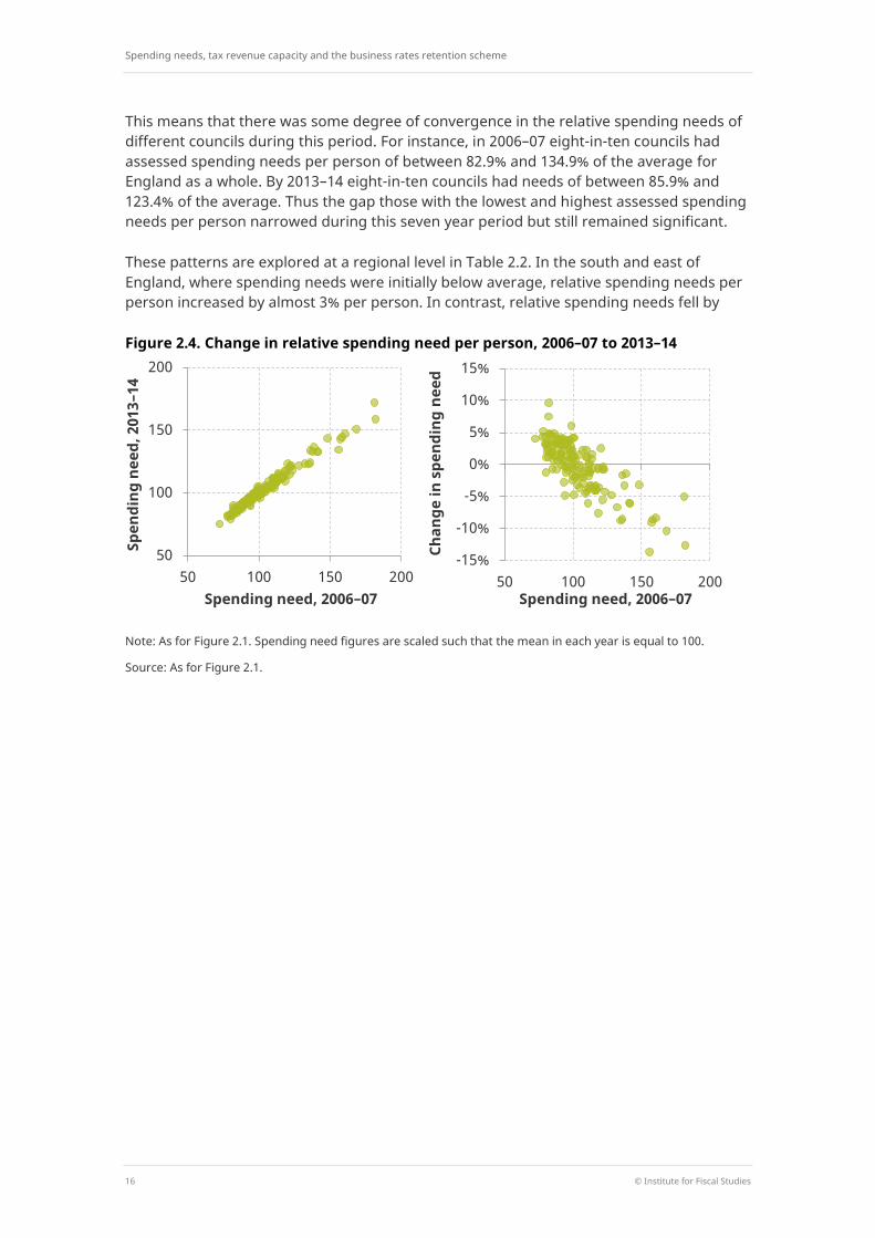
In Figure 2.4, we show two graphs illustrating the relationship between each council’s spending need in 2006–07 and in 2013–14. The graph on the left compares a council’s spending needs per person in 2006–07, the first year for which we can construct a consistent measure, with its level seven years later in 2013–14. The two measures are highly correlated, demonstrating that assessed relative spending need was highly persistent over this period.
However, the graph on the right shows that there was a significant negative correlation between assessed needs per person in 2006–07 and the subsequent change in spending needs per person. For instance, the tenth of councils with the highest assessed spending need per person in 2006–07 saw their relative needs fall by on average 7.3% by 2013–14 (although their absolute needs may still have risen). On the other hand the tenth with the lowest initial needs saw their relative needs rise by 3.7%.
6 Phillips and Simpson (2017) show that the concentration of older people in less deprived parts of the country
plays an important role in explaining the lack of correlation between the share of 65s and overs and social care spending.
7 Throughout this report, we confine ourselves to using measures of relative rather than absolute spending need. Estimates of the ‘funding gap’, which implicitly consider measures of absolute need, have been produced at various points by the Local Government Association. See, for example, Local Government Association (2018).
Spending needs, tax revenue capacity and the business rates retention scheme
16 © Institute for Fiscal Studies
This means that there was some degree of convergence in the relative spending needs of different councils during this period. For instance, in 2006–07 eight-in-ten councils had assessed spending needs per person of between 82.9% and 134.9% of the average for England as a whole. By 2013–14 eight-in-ten councils had needs of between 85.9% and 123.4% of the average. Thus the gap those with the lowest and highest assessed spending needs per person narrowed during this seven year period but still remained significant.
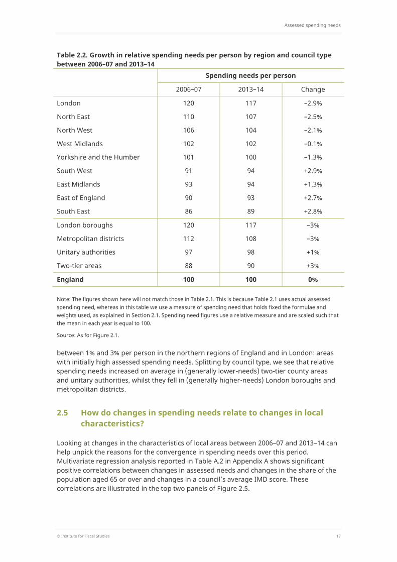
These patterns are explored at a regional level in Table 2.2. In the south and east of England, where spending needs were initially below average, relative spending needs per person increased by almost 3% per person. In contrast, relative spending needs fell by
Figure 2.4. Change in relative spending need per person, 2006–07 to 2013–14
Note: As for Figure 2.1. Spending need figures are scaled such that the mean in each year is equal to 100.
Source: As for Figure 2.1.
50
100
150
200
50 100 150 200
Spen
ding
nee
d, 2
013–
14
Spending need, 2006–07
-15%
-10%
-5%
0%
5%
10%
15%
50 100 150 200
Chan
ge in
spe
ndin
g ne
ed
Spending need, 2006–07
Assessed spending needs
© Institute for Fiscal Studies 17
Table 2.2. Growth in relative spending needs per person by region and council type between 2006–07 and 2013–14
Spending needs per person
2006–07 2013–14 Change
London 120 117 –2.9%
North East 110 107 –2.5%
North West 106 104 –2.1%
West Midlands 102 102 –0.1%
Yorkshire and the Humber 101 100 –1.3%
South West 91 94 +2.9%
East Midlands 93 94 +1.3%
East of England 90 93 +2.7%
South East 86 89 +2.8%
London boroughs 120 117 –3%
Metropolitan districts 112 108 –3%
Unitary authorities 97 98 +1%
Two-tier areas 88 90 +3%
England 100 100 0%
Note: The figures shown here will not match those in Table 2.1. This is because Table 2.1 uses actual assessed spending need, whereas in this table we use a measure of spending need that holds fixed the formulae and weights used, as explained in Section 2.1. Spending need figures use a relative measure and are scaled such that the mean in each year is equal to 100.
Source: As for Figure 2.1.
between 1% and 3% per person in the northern regions of England and in London: areas with initially high assessed spending needs. Splitting by council type, we see that relative spending needs increased on average in (generally lower-needs) two-tier county areas and unitary authorities, whilst they fell in (generally higher-needs) London boroughs and metropolitan districts.
2.5 How do changes in spending needs relate to changes in local characteristics?
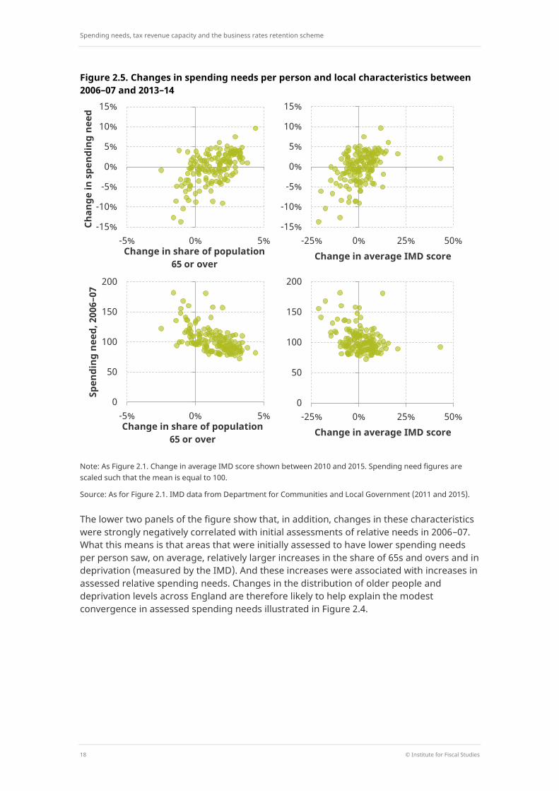
Looking at changes in the characteristics of local areas between 2006–07 and 2013–14 can help unpick the reasons for the convergence in spending needs over this period. Multivariate regression analysis reported in Table A.2 in Appendix A shows significant positive correlations between changes in assessed needs and changes in the share of the population aged 65 or over and changes in a council’s average IMD score. These correlations are illustrated in the top two panels of Figure 2.5.
Spending needs, tax revenue capacity and the business rates retention scheme
18 © Institute for Fiscal Studies
Figure 2.5. Changes in spending needs per person and local characteristics between 2006–07 and 2013–14
Note: As Figure 2.1. Change in average IMD score shown between 2010 and 2015. Spending need figures are scaled such that the mean is equal to 100.
Source: As for Figure 2.1. IMD data from Department for Communities and Local Government (2011 and 2015).
The lower two panels of the figure show that, in addition, changes in these characteristics were strongly negatively correlated with initial assessments of relative needs in 2006–07. What this means is that areas that were initially assessed to have lower spending needs per person saw, on average, relatively larger increases in the share of 65s and overs and in deprivation (measured by the IMD). And these increases were associated with increases in assessed relative spending needs. Changes in the distribution of older people and deprivation levels across England are therefore likely to help explain the modest convergence in assessed spending needs illustrated in Figure 2.4.
-15%
-10%
-5%
0%
5%
10%
15%
-5% 0% 5%
Chan
ge in
spe
ndin
g ne
ed
Change in share of population 65 or over
-15%
-10%
-5%
0%
5%
10%
15%
-25% 0% 25% 50% Change in average IMD score
0
50
100
150
200
-5% 0% 5%
Spen
ding
nee
d, 2
006–
07
Change in share of population 65 or over
0
50
100
150
200
-25% 0% 25% 50% Change in average IMD score
Tax revenue capacity
© Institute for Fiscal Studies 19
3. Tax revenue capacity Councils in England have traditionally relied on a mix of government grants and their own tax revenues for funding. In recent years, the trend has been towards greater reliance on local tax revenues, reflecting both cuts to grants (as part of government austerity measures) and the introduction of the BRRS in 2013–14. This trend is set to continue: the planned increase to 75% business rates retention in 2020–21 will be accompanied by the abolition of the general and public health grants. A further increase to 100% retention would require additional grants – such as the Improved Better Care Fund for social care – to be rolled into the BRRS and/or additional spending responsibilities to be devolved to local government. This would mean councils would be dependent on council tax and business rates for the vast majority of their non-schools spending.
In this context, this chapter examines how the potential revenue from council tax and business rates varies around England, and how this has changed over time.
3.1 How do we measure tax revenue capacity?
Councils’ tax revenues can vary due to differences in the size of local tax bases and differences in the tax rates applied to them. Our focus is on the former: how the capacity of different council areas to generate business rates and council tax revenues varies, as opposed to differences in revenues that result from variation in tax rates.
During the period we examine, business rates were set centrally, so there was no variation in tax rates across councils. We therefore use actual business rates revenues in each area as the basis of our measure of business rates revenue capacity. However, we adjust these revenues by adding back in the value of any discretionary business rates reliefs granted by councils. This allows us to abstract from these decisions and ensure consistency across councils in our measurement of revenue capacity. In addition, when examining changes in tax revenue capacity, we strip out the estimated effects of the 2010 revaluation of non-domestic properties.8 We do this so that our analysis reflects the treatment of revaluation under the BRRS – where the immediate impact of revaluation on revenues is stripped out of the revenues actually retained by councils.9 A number of other smaller adjustments are also made to ensure consistency over time.10
8 Unlike for the 2017 revaluation, we do not have exact figures on the effect of the 2010 revaluation on the
rateable value of properties in each council area. Instead we estimate this by assuming that any difference between council-level and national-level changes in rateable values between 2009–10 and 2010–11 is as a result of revaluation. In practise, some of these changes will reflect differential changes in the stock of non-domestic property of different council areas in 2010-11 as well as changes as a result of revaluation. However, with changes in the stocks of non-domestic property in 2010-11 on average relatively small compared to changes in the stock over the seven year period as a whole, any resulting measurement error is likely to be small as well.
9 This is done by adjusting the top-ups and tariffs that are used to redistribute revenues between councils under the BRRS (Section 4.2 discusses tariffs and top-ups in more detail). Revaluation can affect the revenues councils retain in subsequent years though: any new development (or demolition) has a bigger or smaller effect on revenues if values are higher or lower in a council area than prior to the revaluation.
10 In particular, when examining changes in business rates revenue capacity over time, we estimate and strip out the effect of changes to the empty properties relief and small business relief schemes. We do this because under the BRRS, councils are compensated for changes in their business rates income that result from policy changes made by central government. We also strip out the effects of transitional relief provided to

Spending needs, tax revenue capacity and the business rates retention scheme
20 © Institute for Fiscal Studies
On the other hand, councils have (some) discretion over the council tax rates they charge.11 As a result, council tax rates vary significantly across England. For instance, in 2006–07, the first year that we analyse, rates for a Band D property varied from £648.24 in Wandsworth to £1,483.56 in Newark & Sherwood. In one-in-ten billing areas (which are lower-tier shire districts in two-tier areas) the Band D rate was £1,191 or less, whilst in another one-in-ten it was £1,375 or more. By 2015–16, the range had widened further – the lowest Band D rate was £674.16 whilst the highest had risen to £1,756.44. A significant proportion of the variation in council tax revenues therefore reflects differences in council tax rates as opposed to differences in council tax bases. To calculate our measure of council tax revenue capacity, we therefore apply the national average council tax rate to each council area’s council tax base.12
Our overall measure of tax revenue capacity is the sum of business rates and council tax revenue capacity. As in Chapter 2, we combine shire districts (lower-tier authorities) with their respective counties (upper-tier authorities) in order to be able to compare revenue capacity between two-tier areas and the rest of England.
3.2 How does tax revenue capacity vary around England?
We first examine the extent to which tax revenue capacity varies between councils. Figure 3.1 shows this variation to be substantial. Our estimate of revenue-raising capacity13 per person in 2015–16 is only around £550 for Lewisham, whilst that for Westminster is around 14 times higher at more than £7,500 (and is off the scale of Figure 3.1!). All in all, 21 council areas – almost one-in-seven – are estimated to have had a tax revenue capacity of more than £1,000 per person, while at the other end of the spectrum, a similar number had a tax revenue capacity of less than £650 per person.
Councils in London are over-represented among both those with the lowest tax revenue capacities (including the three with the very lowest) and the highest tax revenue capacities (including the top seven). This reflects the fact that the business rates tax base is highly concentrated in a few boroughs in London (with others having relatively little business property) and the fact that in 1991 (the year on which council tax bandings are based) some parts of London had very high residential property prices and others much lower prices (since then, prices have risen strongly across London).
ratepayers at revaluation as these are also stripped out from the business rates revenues retained under the BRRS.
11 Council tax in the UK is charged according to which of eight valuation bands a property is assessed to be in. Councils have some discretion over the overall level of council tax charged, but the ratios between the charges applied to different bands (and the allocation of property to bands) are centrally fixed.
12 The average council tax rate applied excludes that raised via parish precepts and for fire and police services. To do this, in areas where the county (or unitary authority) council is responsible for fire, we subtract the average amount in council tax charged by separate fire authorities in areas where they exist, before including the county in our calculation of average council tax rates. As with business rates, we make some further adjustments for the sake of consistency when examining changes over time. In particular, when examining changes in revenue capacity over time, we add back reductions in councils’ tax bases as a result of their council tax reduction schemes (which pay council tax bills for those with low incomes) for years between 2013–14 and 2015–16. This is to make figures consistent with the prior period before the localisation of these schemes. However, when examining the level of council tax revenue capacity in 2015–16, we do not make this adjustment.
13 We use ‘revenue-raising capacity’ and ‘tax revenue capacity’ interchangeably in this report.

Tax revenue capacity
© Institute for Fiscal Studies 21
Figure 3.1. Variation in tax revenue capacity per person, 2015–16
Note: Excludes Westminster and City of London for scaling reasons.
Source: Authors’ calculations using Department for Communities and Local Government (2013b), Office for National Statistics (2015a) and Chartered Institute of Public Finance and Accountancy (2016).
Figure 3.2. Relationship between tax revenue capacity and population, 2015–16
Source: As for Figure 3.1.
£0
£500
£1,000
£1,500
£2,000
£2,500
£3,000 Re
venu
e-ra
isin
g ca
paci
ty
London borough Metropolitan borough
Unitary authority County council
0.0%
0.5%
1.0%
1.5%
2.0%
2.5%
3.0%
3.5%
4.0%
4.5%
0.0% 0.5% 1.0% 1.5% 2.0% 2.5% 3.0%
Shar
e of
nat
iona
l rev
enue
-rai
sing
ca
paci
ty
Share of national population
London borough Metropolitan borough Unitary authority County council

Spending needs, tax revenue capacity and the business rates retention scheme
22 © Institute for Fiscal Studies
Table 3.1. Revenue-raising capacity per person, 2015–16, by region Business rates Council tax Total
Total Mean=100 Total Mean=100 Total Mean=100
London £798 182 £448 105 £1,246 144
South East £402 92 £474 111 £875 101
East of England £378 86 £447 105 £825 96
South West £363 83 £455 107 £818 95
North West £387 89 £391 92 £778 90
Yorkshire & the Humber
£370 85 £385 90 £755 87
West Midlands £356 81 £395 93 £751 87
North East £329 75 £382 90 £712 82
East Midlands £318 73 £394 93 £712 82
England £438 100 £426 100 £863 100
Source: As for Figure 3.1.
The particular characteristics of London mean the pattern of revenues differs quite significantly from that in the rest of the country. For instance, Figure 3.2 shows that excluding London boroughs, there is a strong correlation between councils’ population shares and their shares of national tax revenue capacity: in a simple linear regression, population can ‘explain’ 97% of the variation in tax revenue capacity outside London. On the other hand, for London, there is no statistically significant relationship between population and tax revenue capacity. And a number of London boroughs stand out as significant outliers, with tax revenue capacity shares much higher than population shares. These outliers mean that across England as a whole, population can ‘explain’ 61% of the variation in revenue-raising capacity in 2015–16: a lower share than for assessed spending needs (95%).
Table 3.1 shows how estimated tax revenue capacity varied by region in 2015–16, both separately by business rates and council tax, and combined. Local tax revenue capacity in London was more than 40% higher per person than the average for England as a whole, and more than £350 per person higher than in any other region. The gap between London and the rest of the country was greater than the variation between regions in the rest of the country (the difference between the South East and the East Midlands and North East was £163).
This gap between London and the rest of England reflects business rates revenue capacity: revenue capacity for this tax is estimated to be around twice as high per person in London as in the next-highest region (the South East). And all regions bar London have a business rates revenue capacity per person that is below the average for England as a whole. On the other hand, council tax revenue capacity per person is estimated to be higher in the South East and South West of England than in London. And there is a more
Tax revenue capacity
© Institute for Fiscal Studies 23
even spread of regions with above-average council tax revenue capacity (in the south) and below-average capacity (in the midlands and north).
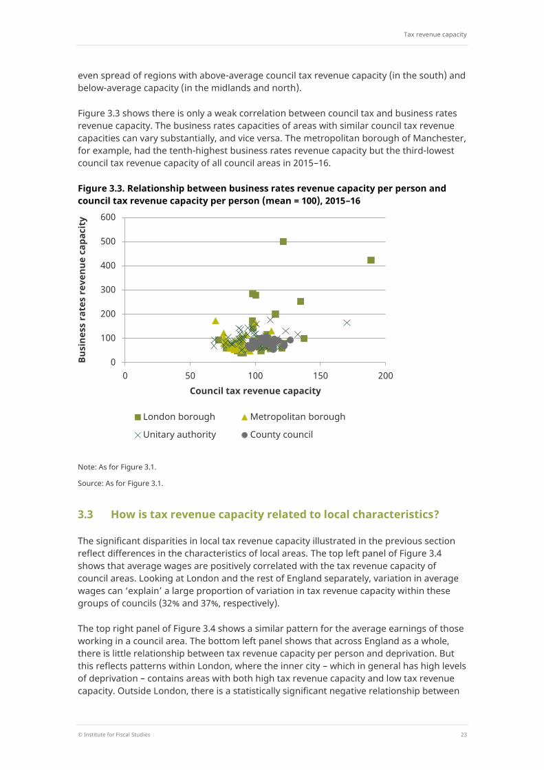
Figure 3.3 shows there is only a weak correlation between council tax and business rates revenue capacity. The business rates capacities of areas with similar council tax revenue capacities can vary substantially, and vice versa. The metropolitan borough of Manchester, for example, had the tenth-highest business rates revenue capacity but the third-lowest council tax revenue capacity of all council areas in 2015–16.
Figure 3.3. Relationship between business rates revenue capacity per person and council tax revenue capacity per person (mean = 100), 2015–16
Note: As for Figure 3.1.
Source: As for Figure 3.1.
3.3 How is tax revenue capacity related to local characteristics?
The significant disparities in local tax revenue capacity illustrated in the previous section reflect differences in the characteristics of local areas. The top left panel of Figure 3.4 shows that average wages are positively correlated with the tax revenue capacity of council areas. Looking at London and the rest of England separately, variation in average wages can ‘explain’ a large proportion of variation in tax revenue capacity within these groups of councils (32% and 37%, respectively).
The top right panel of Figure 3.4 shows a similar pattern for the average earnings of those working in a council area. The bottom left panel shows that across England as a whole, there is little relationship between tax revenue capacity per person and deprivation. But this reflects patterns within London, where the inner city – which in general has high levels of deprivation – contains areas with both high tax revenue capacity and low tax revenue capacity. Outside London, there is a statistically significant negative relationship between
0
100
200
300
400
500
600
0 50 100 150 200
Busi
ness
rat
es r
even
ue c
apac
ity
Council tax revenue capacity
London borough Metropolitan borough
Unitary authority County council

Spending needs, tax revenue capacity and the business rates retention scheme
24 © Institute for Fiscal Studies
tax revenue capacity per person and deprivation (variation in which ‘explains’ 27% of the variation in tax revenue capacity per person).
Figure 3.4. Relationship between tax revenue capacity per person (mean = 100) and various local characteristics, 2015–16
Note: City of London (residents) and Isles of Scilly (workers and residents) are excluded from the graphs (and calculations in the text) on average earnings due to insufficient sample sizes for average earnings. Westminster is excluded for scaling reasons. City of London is excluded from the graph on IMD for scaling reasons. City of London and Westminster are excluded from the graph showing GVA for scaling reasons. Figures on average earnings and GVA are scaled such that the mean of each variable is equal to 100.
Source: As for Figures 2.2 and 3.1. GVA data from Office for National Statistics (2016).
Finally, the bottom right panel shows that there is a strongly statistically significant and positive relationship between local gross value added (GVA) per person – a measure of overall local economic output – and tax revenue capacity. Across England as a whole, variation in GVA per person ‘explains’ 89% of the variation in tax revenue capacity per person in a simple linear regression. The strength of this relationship is driven by councils in London which sometimes have very high levels of GVA and revenues per person, skewing the overall picture. Even so, excluding London boroughs, variation in GVA per person ‘explains’ a somewhat more modest (but still significant) 56% of the variation in
0
100
200
300
400
0 100 200 Reve
nue-
rais
ing
capa
city
Median earnings of residents
0
100
200
300
400
0 100 200 Median earnings of workers
0
100
200
300
400
0 20 40 60
Reve
nue-
rais
ing
capa
city
Average IMD score
0
100
200
300
400
0 200 400
GVA per person

Tax revenue capacity
© Institute for Fiscal Studies 25
tax revenue capacity per person. This suggests that in the long run, there is likely a fairly strong relationship between growth in the local economy and growth in the local tax revenue capacity. We examine whether such a relationship holds in the short-to-medium term as well in Section 3.5, below.
Using multivariate regression analysis, it is possible to examine the relationships between tax revenue capacity and various local characteristics in combination in order to gain further insight into variation in revenue-raising capacity across councils. The results of a number of such regressions are shown in Table A.3 in Appendix A. The key findings are the following:
When both the average earnings of residents and workers are included, only the former are statistically significant. In other words, variation in the average earnings of workers explains little of the remaining variation in tax revenue capacity once the average earnings of residents have been accounted for.
When controlling for GVA in a regression of revenue-raising capacity on average earnings of residents, only GVA is statistically significant. This suggests that earnings may be informative about variation in revenue-raising capacity simply as a result of their being an indicator of overall economic activity rather than having a more direct link to tax revenue capacity.
3.4 How has tax revenue capacity changed over time?
As we discuss further in Section 4.2, it is changes in tax revenue capacity over time (rather than initial variation in the levels of tax revenue capacity) that would likely matter more for funding out-turns under a 100% BRRS. Table 3.2 shows changes in tax revenue capacity by region between 2006–07 and 2015–16, after stripping out our estimate of the effect of the 2010 business rates revaluation on councils’ tax revenue capacity (as happens under the BRRS).
Perhaps surprisingly, tax revenue capacity per person grew least quickly between 2006–07 and 2015–16 in London. This may reflect several factors. First, we have stripped out the effect of the 2010 business rates revaluation, and council tax bands are still based on 1991 residential property prices, so the figures do not reflect the well-documented increase in the relative value of properties in London. Second, London experienced much faster growth in population (14.2%) than growth in household numbers (8.4%) over this period, whereas growth in these was more or less equal in the rest of England. The increase in average household size in London would tend to push down council tax revenue capacity per person.
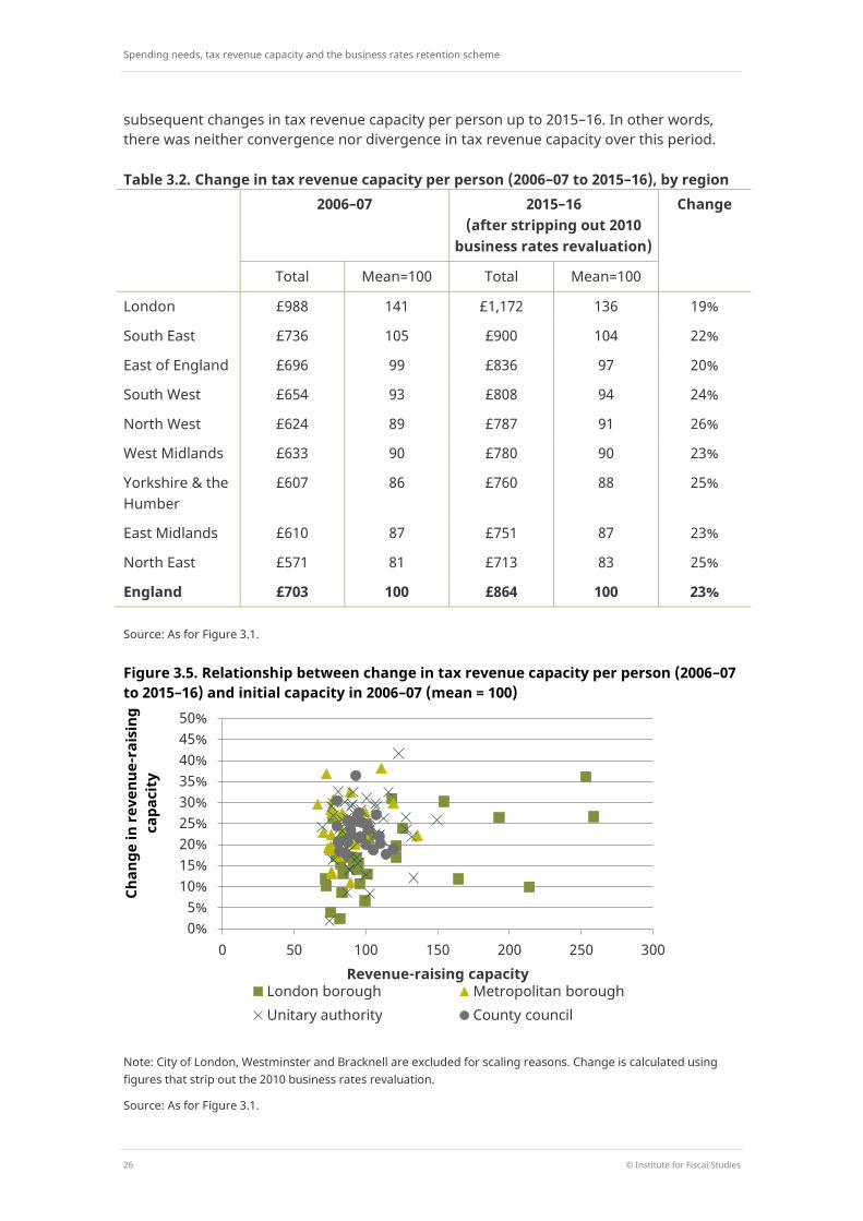
Table 3.2 also shows that, more generally, those regions with higher tax revenue capacity per person in 2006–07 (London, the South East and East of England) saw slower growth in tax revenue per capacity over the subsequent nine years. However, although a regional perspective is useful, the local government finance system operates at a council level. Figure 3.5 shows that there was significant variation in changes in tax revenue capacity at the council level. Around one-in-ten councils saw their tax revenue capacity increase by 13% or less, while another one-in-ten saw it increase by 30% or more. But there was no statistically significant relationship between initial revenue capacity per person and the
Spending needs, tax revenue capacity and the business rates retention scheme
26 © Institute for Fiscal Studies
subsequent changes in tax revenue capacity per person up to 2015–16. In other words, there was neither convergence nor divergence in tax revenue capacity over this period.
Table 3.2. Change in tax revenue capacity per person (2006–07 to 2015–16), by region 2006–07 2015–16
(after stripping out 2010 business rates revaluation)
Change
Total Mean=100 Total Mean=100
London £988 141 £1,172 136 19%
South East £736 105 £900 104 22%
East of England £696 99 £836 97 20%
South West £654 93 £808 94 24%
North West £624 89 £787 91 26%
West Midlands £633 90 £780 90 23%
Yorkshire & the Humber
£607 86 £760 88 25%
East Midlands £610 87 £751 87 23%
North East £571 81 £713 83 25%
England £703 100 £864 100 23%
Source: As for Figure 3.1.
Figure 3.5. Relationship between change in tax revenue capacity per person (2006–07 to 2015–16) and initial capacity in 2006–07 (mean = 100)
Note: City of London, Westminster and Bracknell are excluded for scaling reasons. Change is calculated using figures that strip out the 2010 business rates revaluation.
Source: As for Figure 3.1.
0% 5%
10% 15% 20% 25% 30% 35% 40% 45% 50%
0 50 100 150 200 250 300
Chan
ge in
rev
enue
-rai
sing
ca
paci
ty
Revenue-raising capacity London borough Metropolitan borough Unitary authority County council
Tax revenue capacity
© Institute for Fiscal Studies 27
3.5 How do changes in tax revenue capacity relate to changes in local characteristics?
We now turn to examining how changes in local tax revenue capacity relate to changes in local economic activity. This is particularly interesting given that one of the aims of policies such as the BRRS is to incentivise councils to grow their local economies.14,15
First, we look at the link between changes in tax revenue capacity and changes in population. At the beginning of Section 3.3, we saw that the level of revenue raising capacity was strongly linked to population in 2015–16, especially outside of London. However, the link between changes in revenue capacity and changes in population is much less strong. Although there was a statistically significant positive correlation between the two for changes between 2006–07 and 2015–16, population growth only accounts for 18% of the variation in changes in overall tax revenue capacity. For council tax only, the relationship is stronger: population growth accounts for 39% of the variation in changes in council tax revenue capacity. On the other hand, for business rates, population growth only accounts for 3% of the variation in changes in tax revenue capacity during the period 2006–07 to 2015–16. This suggests that increasing the dependence of councils’ funding on changes in local business rates revenues – as under the BRRS – exposes councils to higher risks of substantial changes in revenues per person.
Focusing more specifically on business rates revenue capacity, Figure 3.6 shows how changes in the rateable value of the non-domestic property in different council areas (the business rates tax base) between 2010–11 and 2015–16 relate to changes in two measures of local economic activity: GVA per person and the number of workers in a council area per resident of that council area.
It is clear that there is no correlation between changes in the business rates tax base and either variable. Because this was a period during which constant (2008) property values were used to calculate business rates bills, this means that there was no relationship between changes in the quantity and physical quality of non-domestic space and changes in these broader measures of local economic performance.
Figure 3.7 shows that, in contrast, there was a statistically significant positive relationship between changes in GVA and in the number of workers per resident and the change in assessed rateable values as a result of the 2017 revaluation (which rebased values to 2015 levels). In other words, those areas that saw larger increases in their assessed values at revaluation tended to see faster GVA and workforce growth between 2010 and 2015. We find that a 1 percentage point increase in GVA growth per capita over this period was associated with 0.3% increase in rateable values at the 2017 revaluation (although of course this correlation does not necessarily imply a causal link).
However, as already mentioned, under the BRRS, the immediate impact of revaluations on councils’ retained revenues is stripped out. This significantly reduces the extent to which councils gain or lose as a result of changes in assessed values. Instead, they gain or lose largely as a result of changes in the quantity and physical quality of non-domestic
14 Department for Communities and Local Government, 2012. 15 Separate IFS research, joint with PwC and the Local Government Information Unit, has found that those
councils that are more optimistic about business rates retention tend to be those that have experienced strong growth in GVA – suggesting that councils see economic growth as integral to ‘winning’ from the business rates retention system. See Amin-Smith et al. (2017).

Spending needs, tax revenue capacity and the business rates retention scheme
28 © Institute for Fiscal Studies
property in their area, which, as Figure 3.6 shows, has not been correlated with changes in broader economic conditions in recent years. In light of this, even if business rates retention provided an effective incentive for councils to boost the supply of non-domestic property in their area, it is not clear that this would necessarily translate into broader improvements in local economic conditions.
Figure 3.6. Correlation between change in rateable value per person and change in local characteristics, between 2010–11 and 2015–16
Source: As for Figure 3.1. GVA data from Office for National Statistics (2016). Workplace population data from Office for National Statistics (2015b).
Figure 3.7. Correlation between change in rateable value per person at 2017 revaluation and change in local characteristics between 2010–11 and 2015–16
Source: GVA data from Office for National Statistics (2016). Workplace population data from Office for National Statistics (2015b). Data on changes in rateable values at revaluation from Valuation Office Agency (2017).
The fact that changes in property values are positively correlated with changes in broader economic conditions may suggest that allowing councils to gain or lose as a result of revaluation would provide a more effective incentive for growth. This has been suggested by the Centre for Cities (2017), for instance. However, it would also expose councils to potentially large changes in their business rates revenues at the time of revaluation. And it could incentivise councils to restrict the supply of property to push up property values (rather than take action to increase the demand for property).
-20%
-10%
0%
10%
20%
30%
-20% 0% 20% 40%
Chan
ge in
rat
eabl
e va
lue
per
pers
on
Change in GVA per person
-20%
-10%
0%
10%
20%
30%
-40% -20% 0% 20% 40% 60%
Change in worker–resident ratio
-30%
-20%
-10%
0%
10%
20%
30%
40%
-50% 0% 50%
Chan
ge in
rat
eabl
e va
lue
per
pers
on
Change in GVA per person -30%
-20%
-10%
0%
10%
20%
30%
40%
-30% -10% 10% 30% 50%
Change in worker–resident ratio

Analysis of 100% rates retention
© Institute for Fiscal Studies 29
4. Analysis of 100% rates retention In this chapter, we bring our analysis of assessed spending needs and tax revenue capacity together. In particular, we first examine the correlation between these variables in 2013–14, which illustrates the key role redistribution of revenues between council areas would play under a system of 100% business rates retention (as it does under 50% retention). We then model the extent to which councils’ shares of retained revenue could have diverged from their shares of assessed spending needs under 100% rates retention if it had operated during the period 2006–07 to 2013–14. This gives us a sense of the potential scale of funding divergences that could arise if a 100% rates retention system were introduced in future. It also allows us to analyse how key features of the BRRS – the safety net and the share of revenues allocated to upper and lower tiers of local government in areas with two tiers – affect the scope for funding divergences.
4.1 Revenue capacity and spending needs
Figure 4.1 shows the relationship between tax revenue capacity and assessed relative spending needs per person as of 2013–14. Note that as in Chapters 2 and 3, we normalise reported figures so that the mean for each variable is 100.
Figure 4.1. Relationship between revenue-raising capacity and spending need per person (mean = 100), 2013–14
Note: Excludes Isles of Scilly, Westminster and City of London (the latter two for scaling reasons).
Source: Authors’ calculations using Department for Communities and Local Government (2013a and 2013b), Office for National Statistics (2015a) and Chartered Institute of Public Finance and Accountancy (2016).
Across England as a whole, there was a statistically significant positive correlation between assessed spending needs and tax revenue capacity per person in 2013–14. However, this was driven by patterns of need and revenue in London: excluding London boroughs, there was a statistically significant negative correlation between needs and
0
50
100
150
200
250
300
350
50 75 100 125 150 175
Reve
nue-
rais
ing
capa
city
Spending need
London borough Metropolitan borough
Unitary authority County council
Spending needs, tax revenue capacity and the business rates retention scheme
30 © Institute for Fiscal Studies
revenue capacity per person. In other words, councils outside London with relatively high assessed spending needs were likely to have below-average tax revenue capacity, and vice versa. And for London, where higher levels of spending needs were associated with above-average tax revenue capacity, there were still large discrepancies between the two for some councils. For instance, Lewisham’s share of tax revenue capacity is estimated to have been around half its share of assessed needs, while Westminster’s share is estimated to be around six times its share of assessed needs.
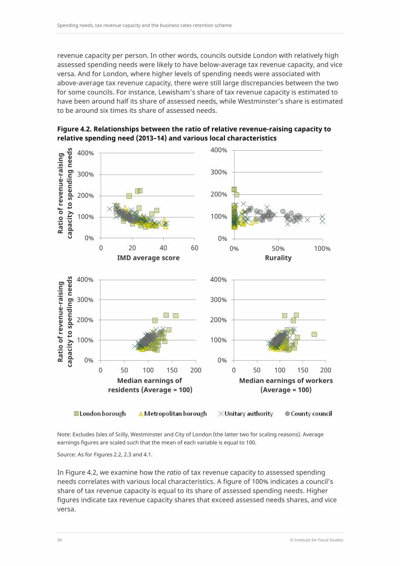
Figure 4.2. Relationships between the ratio of relative revenue-raising capacity to relative spending need (2013–14) and various local characteristics
Note: Excludes Isles of Scilly, Westminster and City of London (the latter two for scaling reasons). Average earnings figures are scaled such that the mean of each variable is equal to 100.
Source: As for Figures 2.2, 2.3 and 4.1.
In Figure 4.2, we examine how the ratio of tax revenue capacity to assessed spending needs correlates with various local characteristics. A figure of 100% indicates a council’s share of tax revenue capacity is equal to its share of assessed spending needs. Higher figures indicate tax revenue capacity shares that exceed assessed needs shares, and vice versa.
0%
100%
200%
300%
400%
0 20 40 60
Rati
o of
rev
enue
-rai
sing
ca
paci
ty t
o sp
endi
ng n
eeds
IMD average score
0%
100%
200%
300%
400%
0% 50% 100% Rurality
0%
100%
200%
300%
400%
0 50 100 150 200
Rati
o of
rev
enue
-rai
sing
ca
paci
ty t
o sp
endi
ng n
eeds
Median earnings of residents (Average = 100)
0%
100%
200%
300%
400%
0 50 100 150 200 Median earnings of workers
(Average = 100)
Analysis of 100% rates retention
© Institute for Fiscal Studies 31
The top left panel shows that excluding London, there is a clear pattern of higher levels of deprivation being associated with lower ratios of tax revenue capacity to spending needs. We find that the tenth of councils with the highest levels of deprivation had an average ratio of tax revenue capacity to assessed spending need of 70%. That means, on average, their share of tax revenues was 30% lower than their share of assessed spending needs. On the other hand, the tenth of councils with the lowest levels of deprivation had an average ratio of 131%. That is, a share of revenues that is, on average, 31% higher than their share of assessed needs.
The lower two panels show that higher earnings of both residents and workers are associated with higher ratios of tax revenue capacity to spending needs outside London. In particular, a 1 percentage point increase in the median earnings of residents relative to the national average is associated with a 1.8 percentage point increase in the ratio of tax revenue capacity to assessed spending need outside London. A 1 percentage point relative increase in earnings of workers is associated with a 1.4 percentage point increase in the ratio outside London. These patterns are as one would expect given the needs assessment (which includes characteristics linked to deprivation such as benefit claims and ill health) and the property tax base of councils (with, for instance, higher-income people likely to be living in areas with properties in higher council tax bands).
Within London, though, there is no relationship between these characteristics and the ratio of tax revenue capacity to spending needs. This likely reflects the complex patterns of deprivation, earnings and property tax bases in London. Some areas reflect national patterns. For instance, areas such as Richmond-upon-Thames and Barnet have low levels of deprivation and assessed needs and high tax revenue capacity. And areas such as Barking & Dagenham, Lewisham and Newham have high levels of deprivation and assessed needs and low tax revenue capacity. But other areas, such as Westminster and Camden, buck the national trend, having high levels of deprivation, assessed needs and tax revenue capacity.
4.2 Simulating funding under 100% business rates retention
The negative correlation and large gaps between tax revenue capacity and assessed spending needs per person suggest that, without significant redistribution of revenues, there would be big divergences in different councils’ ability to fund local public services. In particular, more deprived areas would typically receive a lower share of revenues than their share of spending needs, and vice versa for less deprived areas.
In this context, if the BRRS meant councils actually retained 50% (or 75% or 100%) of local rates revenues, then it would mean large divergences between the revenues and assessed needs of different councils. However, the BRRS does not work like this. Instead, when the system was set up in April 2013, an assessment was made of how much business rates revenue each council would need (given how much it would have received under the previous grant-funding system) and how much revenues it would likely receive in 2013–14 given the share of local revenues allocated to it. Those councils for which revenue needs were less than expected revenues were made to pay a ‘tariff’ equal to this difference. Those councils for which revenue needs were more than expected revenues received a ‘top-up’ to make up this difference. These tariffs and top-ups therefore redistribute business rates revenues from areas that in 2013–14 were estimated to have high revenues and/or low needs to areas with low revenues and/or high needs.
Spending needs, tax revenue capacity and the business rates retention scheme
32 © Institute for Fiscal Studies
Since 2013–14, these tariffs and top-ups have been indexed in line with RPI (Retail Prices Index) inflation. This means that councils have an incentive to grow their business rates revenues: they gain or lose up to 50% of the real-terms change in business rates revenues in their area. But it also means that their share of retained revenues can diverge from their share of revenue needs. This will happen whenever there are real-terms changes in business rates revenues, even if those changes are the same across the country. This is because the redistributive tariffs and top-ups will become smaller (or larger) relative to underlying business rates revenues when those revenues are growing (or shrinking) in real terms. But the divergences between retained revenues and spending needs will, in general, be larger if business rates revenues and relative spending needs are changing differently for different councils. Furthermore, all else equal, the potential scale of divergences would be greater under 100% than 50% business rates retention.
We do not know how councils’ tax revenues and spending needs will change in future. So to get a sense of the potential divergences that could arise under a 100% BRRS, we simulate such a system using our data on tax revenue capacity and assessed spending needs from 2006–07 to 2013–14.
Modelling 100% retention for the period 2006–07 to 2013–14 We model 100% retention at the level of individual councils, which is the level at which the BRRS actually operates. This means that rather than pooling tax revenues and assessed spending needs at the upper-tier level in areas with two-tier local government as we have done so far (to allow consistent comparisons with single-tier areas), we need to apportion them between both lower and upper tiers. For assessed spending needs, this is straightforward: separate assessments are provided for each tier. Apportionment of tax revenue capacity is more complex; our approach is set out in Box 4.1.
Box 4.1. Apportioning tax revenue capacity in two-tier areas
We use different approaches to apportion business rates and council tax:
Business rates. These are apportioned according to the shares allocated to lower and upper tiers under the BRRS being modelled. For instance, in our baseline scenario, we scale up the tier shares used in the 50% BRRS: 80% is allocated to lower-tier districts and 18% allocated to upper-tier counties (the remaining 2% of retained revenues is assumed to be allocated to fire services, as under the 50% BRRS). We also test the sensitivity of trends in retained revenues to alternative tier shares.
Council tax. We first calculate the average share of council tax revenues that goes to lower-tier districts and upper-tier counties across England as a whole.a We then apply these shares to the council tax revenue capacities of each lower-tier area – i.e. the council tax revenues that would be raised in an area if the national average tax rate were applied – to apportion revenue capacity between tiers.
a Before calculating these averages, a proportion equal to the average proportion of council tax charged by independent fire authorities is subtracted for counties responsible for their own fire services.

Analysis of 100% rates retention
© Institute for Fiscal Studies 33
Our analysis is based on the tax revenue capacity of councils (assuming they set a common council tax rate) as opposed to actual tax revenues. We do this to focus on the divergences that would have opened up because of changes in local tax bases and assessed spending needs, rather than because of differences in the council tax rates that councils choose to set.
The precise details of what a 100% BRRS would look like if it were rolled out nationally have not been set out. We therefore base the system we model on consultation documents and the 50% BRRS:16
Each council retains its council tax revenue (capacity) in full.
Business rates revenues from properties on the local list are allocated in full to councils. In our baseline scenario, 80% of rates revenues are initially allocated to lower-tier district councils and 18% to upper-tier counties. Within London, 60% are allocated to boroughs and 38% to the Greater London Authority (GLA). These shares are then varied in subsequent simulations.
Redistributive tariffs and top-ups are set up to redistribute revenues from areas with high revenues and/or low needs to those with low revenues and/or high needs. They are initially set on the basis of an estimate of each council’s revenues (based on its share of revenues in 2005–06 and 2006–07) and assessed spending needs (in 2006–07), with the aim of fully offsetting differences between the two in the first year of the scheme. However, note that as under the 50% scheme, they will not fully offset the differences even in this first year (because they are based on shares of revenues in both 2005–06 and 2006–07, not just the first year of the scheme, 2006–07).17
These tariffs and top-ups are then indexed in line with RPI inflation each year. They are also adjusted to strip out the effect on business rates revenues of the revaluation of non-domestic property that took effect in 2010–11. This mimics the approach taken in 2017–18 under the 50% BRRS.
We then calculate the retained tax revenue (capacity) of each council after accounting for these tariffs and top-ups and compare it with its assessed spending needs. To do this, we calculate the ratio of each council’s share of the national sum of retained revenues to its share of assessed relative spending needs. We term this the council’s relative funding ratio. It measures the proportion by which a council’s share of retained revenues is higher
16 See Department for Communities and Local Government (2017c). Note that there is one feature of the BRRS
that we have to model a little differently from how it works in reality: appeals. Under the BRRS, councils must make an estimate of how much appeals will reduce their revenues in coming years and make an accounting provision. This provision is deducted from revenues up front, and councils can then draw down on this provision to offset the reduction in revenues when appeals actually materialise. The period we examine (2006–07 to 2013–14) is prior to the introduction of this system: councils did not need to make provisions, so we have no data on how large they would be. Instead, appeals were accounted for when they arose. The 100% BRRS we model therefore accounts for appeals in this way. This will have only marginal effects on the medium-term divergences between revenue capacity and assessed needs we focus on in the discussion of our results. However, it could have a larger effect on the year-to-year changes in retained revenues in our simulations.
17 The tariffs and top-ups were set with reference to revenue shares over two years (2010–11 and 2011–12) under the 50% BRRS because revenue volatility means shares based on a single year may not be representative.
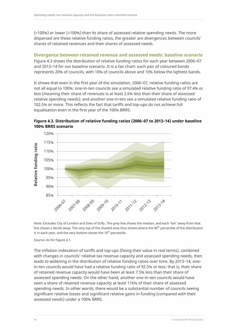
Spending needs, tax revenue capacity and the business rates retention scheme
34 © Institute for Fiscal Studies
(>100%) or lower (<100%) than its share of assessed relative spending needs. The more dispersed are these relative funding ratios, the greater are divergences between councils’ shares of retained revenues and their shares of assessed needs.
Divergence between retained revenue and assessed needs: baseline scenario Figure 4.3 shows the distribution of relative funding ratios for each year between 2006–07 and 2013–14 for our baseline scenario. It is a fan chart: each pair of coloured bands represents 20% of councils, with 10% of councils above and 10% below the lightest bands.
It shows that even in the first year of the simulation, 2006–07, relative funding ratios are not all equal to 100%: one-in-ten councils see a simulated relative funding ratio of 97.4% or less (meaning their share of revenues is at least 2.6% less than their share of assessed relative spending needs); and another one-in-ten see a simulated relative funding ratio of 102.5% or more. This reflects the fact that tariffs and top-ups do not achieve full equalisation even in the first year of the 100% BRRS.
Figure 4.3. Distribution of relative funding ratios (2006–07 to 2013–14) under baseline 100% BRRS scenario
Note: Excludes City of London and Isles of Scilly. The grey line shows the median, and each ‘fan’ away from that line shows a decile away. The very top of the shaded area thus shows where the 90th percentile of the distribution is in each year, and the very bottom shows the 10th percentile.
Source: As for Figure 4.1.
The inflation indexation of tariffs and top-ups (fixing their value in real terms), combined with changes in councils’ relative tax revenue capacity and assessed spending needs, then leads to widening in the distribution of relative funding ratios over time. By 2013–14, one-in-ten councils would have had a relative funding ratio of 92.5% or less: that is, their share of retained revenue capacity would have been at least 7.5% less than their share of assessed spending needs. On the other hand, another one-in-ten councils would have seen a share of retained revenue capacity at least 116% of their share of assessed spending needs. In other words, there would be a substantial number of councils seeing significant relative losses and significant relative gains in funding (compared with their assessed needs) under a 100% BRRS.
85%
90%
95%
100%
105%
110%
115%
120%
Rela
tive
fund
ing
rati
o

Analysis of 100% rates retention
© Institute for Fiscal Studies 35
Table 4.1 shows summary statistics for relative funding ratios for different types of councils, both for 2013–14 and for the period 2007–08 to 2013–14 as a whole. Looking at relative funding ratios over a period of several years is useful because it allows us to rule out a scenario where volatility in revenues (and perhaps spending needs) leads to divergences in relative funding ratios in any single year (such as 2013–14) but not over longer time horizons. Councils could potentially use their reserves to smooth funding across years in the face of year-to-year revenue volatility, but this would not be sustainable in the face of divergence over longer horizons. Comparing the top and bottom panels of the table shows that divergences in relative funding ratios are smaller when averaged over the seven years 2007–08 to 2013–14. However, the differences between the maximum and minimum relative funding ratios are still sizeable.
Table 4.1. Relative funding ratios under baseline 100% BRRS, by council type London
boroughs Metropolitan
districts Unitary
authorities Shire
districts Counties
Relative funding ratio in 2013–14
Minimum 87.2% 96.5% 89.6% 61.0% 91.0%
25th percentile 93.4% 99.6% 94.8% 99.0% 94.4%
Median 95.8% 104.4% 100.0% 104.9% 95.5%
75th percentile 102.9% 107.0% 102.3% 112.2% 96.6%
Maximum 120.3% 114.6% 116.0% 166.4% 101.4%
Average relative funding ratio, 2007–08 to 2013–14
Minimum 94.1% 97.8% 91.1% 78.1% 96.2%
25th percentile 98.0% 99.9% 97.3% 96.8% 97.4%
Median 99.6% 101.5% 99.2% 101.7% 97.8%
75th percentile 101.9% 103.3% 101.2% 105.6% 98.7%
Maximum 107.3% 107.5% 106.0% 140.6% 100.0%
Note: Excludes City of London and Isles of Scilly.
Source: As for Figure 4.1.
Also notable in Table 4.1 are the differences in the distributions of relative funding ratios for the lower-tier shire districts and the upper-tier counties (which subsume shire districts). For example, the councils with the lowest (61.0%) and highest (166.4%) relative funding ratios in 2013–14 are both shire districts. And the interquartile range for shire districts (13.2% = 112.2% minus 99.0%) is around six times as wide as that for counties (2.2% = 96.6% minus 94.4%).
Two factors play a role in this. First, counties cover several shire districts and therefore have significantly larger populations and underlying tax bases than shire districts. This
Spending needs, tax revenue capacity and the business rates retention scheme
36 © Institute for Fiscal Studies
larger scale reduces the variability of both revenue capacity and assessed spending needs. For instance, the building or demolition of a factory would have less impact on the business rates tax base of a county consisting of multiple shire districts than on that of the specific shire district that the factory is located in.
Second, as described in Box 4.1, in our baseline scenario, 80% of business rates revenues are initially allocated to shire districts and 18% to counties. As a result, shire districts typically pay significant inflation-indexed tariffs, whilst counties typically receive significant inflation-indexed top-ups. Hence, shire districts are much more exposed to real-terms changes in local business rates revenues than counties, increasing the scope for divergences between retained revenues and assessed spending needs. This is the flip side of the stronger fiscal incentives provided by their 80% share of business rates revenues.
The impact of changing tier shares on divergences in funding ratios Table 4.2 shows the impact of changing the share of business rates revenues allocated to shire districts and counties in two-tier areas on the distributions of relative funding ratios. Columns 1 and 4 show estimates for the baseline 80%/18% split; columns 2 and 5 show estimates for a 49%/49% split; and columns 3 and 5 show estimates for an 18%/80% split.
Reducing the share of business rates allocated to shire districts significantly reduces the extent of divergences between relative funding ratios for this type of council. For instance, the coefficient of variation of shire districts’ relative funding ratios in 2013–14 falls from 11.98% under the baseline 80% share to 4.48% under an 18% share.18 The inter-quartile range for shire districts for the same year falls from a 13 percentage point difference in relative funding ratios to around a 6 percentage point difference (104.1% minus 98.2%).
Upper-tier counties, of course, see the opposite pattern, although the effect is much smaller: the coefficient of variation of counties’ relative funding ratios in 2013–14 increases from 2.66% under an 18% share of business rates to 3.03% under an 80% share. This relatively small impact reflects two factors:
Subsuming several shire districts, counties have larger, more diverse and hence less variable business rates tax bases.
They also receive a much larger share of council tax revenue capacity than shire districts do. Increasing the share of business rates retained by counties therefore has less of an impact on the variability of overall tax revenue capacity than is the case for shire districts.
Our modelling therefore suggests that decreasing the tier share of shire districts and increasing the tier share of counties would significantly reduce divergences in relative funding ratios for shire districts while leading to only modest increases in divergences among county councils.
Table 4.2 also shows that changing tier shares could also help address another issue evident in our baseline scenario: shire districts doing much better on average under 100% business rates retention than counties (for instance, the median relative funding ratio for
18 The coefficient of variation is defined as the standard deviation divided by the mean.

Analysis of 100% rates retention
© Institute for Fiscal Studies 37
a shire district would have been 104.9% in 2013–14, compared with 95.5% for the median county).
Table 4.2. Relative funding ratios for shire districts and counties, by tier-share scenario Shire districts Counties
80% share
(1)
49% share
(2)
18% share
(3)
18% share
(4)
49% share
(5)
80% share
(6)
Relative funding ratio in 2013–14
Minimum 61.0% 74.0% 87.0% 91.0% 91.3% 91.5%
25th percentile 99.0% 99.1% 98.2% 94.4% 94.8% 95.2%
Median 104.9% 102.7% 100.9% 95.5% 96.0% 96.5%
75th percentile 112.2% 107.9% 104.1% 96.6% 97.6% 98.9%
Maximum 166.4% 143.6% 120.8% 101.4% 103.3% 105.1%
Coefficient of variation
11.98% 8.04% 4.48% 2.66% 3.00% 3.03%
Average relative funding ratio, 2007–08 to 2013–14
Minimum 78.1% 86.4% 93.9% 96.2% 95.8% 95.5%
25th percentile 96.8% 98.5% 100.5% 97.4% 97.3% 97.3%
Median 101.7% 101.0% 100.9% 97.8% 97.9% 98.0%
75th percentile 105.6% 103.8% 102.1% 98.7% 98.5% 99.2%
Maximum 140.6% 125.4% 111.4% 100.0% 100.6% 101.3%
Coefficient of variation
8.46% 5.33% 2.45% 1.01% 1.24% 1.55%
Note: As for Table 4.1.
Source: As for Figure 4.1.
The reason for this is that allocating an 80% share of business rates to districts means that they retain a high proportion of any real-terms change in business rates revenues. In particular, if business rates revenues grow in real terms, as was the case between 2006–07 and 2013–14, the amount retained after paying inflation-linked tariffs increases. And, in contrast, counties’ 18% share of business rates in our baseline scenario means that they receive only a small proportion of the real-terms change in business rates revenues.

Spending needs, tax revenue capacity and the business rates retention scheme
38 © Institute for Fiscal Studies
Instead, they rely on inflation-linked top-ups for a significant proportion of their retained tax revenue capacity. These would be shrinking relative to business rates revenues.19
Decreasing shire districts’ share and increasing counties’ share of business rates revenues would mean counties capture a larger share of the real-terms increase in business rates revenues. This would prevent counties’ share of retained revenues falling when business rates revenues are growing in real terms. Table 4.2 shows that this would have reduced the gap between average performance of shire districts and counties under a 100% BRRS in the period between 2006–07 and 2013–14. For instance, under 18%:80% tier shares, the median relative funding ratio for a shire district would have been 100.9% and that for counties 96.5% in 2013–14.
However, this does not necessarily mean that shifting the initial allocation of business rates revenues from shire districts to counties is desirable. For instance, if business rates revenues were to fall in real terms, increasing counties’ tier share would lead to a reduction in their retained revenues (because they would lose at least some of their inflation-indexed top-ups). Changing tier shares would also affect the strength of the financial incentive that shire districts and county councils have to grow local business rates tax bases.
The rationale for the high share allocated to shire districts and low share allocated to counties under the existing 50% scheme is twofold. First, operation of the planning system – perhaps the local service most closely linked to property development – is largely a responsibility of shire districts. Financial incentives may therefore be expected to have the most direct effect on the behaviour of shire districts. Second, it may be more important to insulate counties from variability in business rates revenues due to the important services they are responsible for: notably, children’s and adults’ social services. The appropriate share of business rates to allocate to shire districts and counties under a 100% BRRS would depend upon their ability to capitalise on the financial incentives provided and their ability to bear revenue risk, as well as upon the potential scale of funding divergences that would result from different tier shares.
To what extent does a safety net reduce funding divergence? So far, our modelling of the 100% BRRS has omitted a key element of the 50% scheme: the safety net. Presently, this provides a top-up to the retained business rates revenues of councils seeing particularly large falls in these revenues, to ensure that they do not fall below 92.5% of the (inflation-indexed) amount they were initially assessed to need at the start of the scheme (which is termed their ‘baseline funding’).
In Figure 4.4 and Table 4.3, we show the distribution of relative funding ratios that would have arisen between 2006–07 and 2013–14 if the safety net threshold for the 100% BRRS were set at 97% of baseline funding and tier shares are in our baseline scenario: 80% for
19 The inflation indexation of top-ups and tariffs also has a more general effect when business rates revenues
increase in real terms: less affluent areas with small business rates tax bases and/or high assessed spending needs that rely on top-ups for a significant proportion of their revenue end up with a shrinking share of overall business rates revenues, unless rates revenues grow at a rate greater than the national average. This could be seen as penalising less affluent areas and could be addressed by indexing top-ups and tariffs to growth in national business rates revenues, which would still maintain incentives for councils to grow their tax bases (Amin-Smith et al., 2016).

Analysis of 100% rates retention
© Institute for Fiscal Studies 39
districts and 20% for counties.20 This is the threshold used in existing and planned 100% business rates pilots and suggested in MHCLG’s second consultation on the 100% BRRS.21
Comparing these results with those obtained when there is no safety net (Figure 4.3) shows that the safety net prevents the largest shortfalls of retained revenue capacity relative to assessed relative spending needs. For instance, in 2013–14, one-in-ten councils would have seen a relative funding ratio of 94.1% or less with such a safety net, compared with 92.5% or less without a safety net. And the lowest relative funding ratio would have been 87.1% compared with 61.0% without a safety net.
Figure 4.4. Distribution of relative funding ratios (2006–07 to 2013–14) under our baseline 100% BRRS with a safety net
Note: As for Figure 4.3. Our baseline scenario has tier-shares of 80% for shire districts and 20% for counties.
Source: As for Figure 4.1.
Table 4.3. Distribution of relative funding ratios under baseline 100% BRRS, 2013–14
Without safety net With safety net
Minimum 61.0% 87.1%
10th percentile 92.5% 94.1%
Median 101.5% 101.7%
90th percentile 116.0% 115.8%
Maximum 166.4% 166.1%
Note: As for Table 4.1. Our baseline scenario has tier-shares of 80% for shire districts and 20% for counties.
Source: As for Figure 4.1.
20 And as in our baseline scenario, business rates are initially shared on an 80%/18% basis between shire
districts and counties in two-tier areas. 21 Department for Communities and Local Government, 2017c.
85%
90%
95%
100%
105%
110%
115%
120%
Rela
tive
fun
ding
rat
io

Spending needs, tax revenue capacity and the business rates retention scheme
40 © Institute for Fiscal Studies
However, it is worth noting three things:
If based on the one in operation under the 50% BRRS, a safety net would only protect councils from large real-terms falls in business rates revenues. Safety-net payments are not paid when council tax revenues fall or when assessed relative spending needs increase. This is why one-in-ten councils see their relative funding ratio fall to 94.1% or less despite a safety net threshold of 97%.
A safety net does not prevent large increases in business rates revenues from feeding through into some councils seeing their share of retained revenues substantially exceeding their share of assessed spending needs. While such ‘excess’ revenues may be less problematic from a budgetary management perspective (councils can put additional revenues into reserves but are restricted in their ability to borrow to fund revenue shortfalls), they still contribute to divergences in councils’ abilities to fund local public services.
The insurance against large falls in business rates revenues provided by the safety net comes at a cost. The monetary cost is the safety-net top-ups to ensure retained rates revenues do not fall below 97% of baseline funding. The broader cost is weakened incentives for councils in receipt of such safety-net payments to boost their business rates tax base. This weakening arises because, until underlying retained revenues are back above 97% of baseline funding, every £1 increase in retained revenues is offset by a £1 decrease in safety-net payments. Councils therefore do not gain financially from a marginal increase in business rates revenues.
Alongside safety nets, it will therefore be important to have broader resets of the redistributive tariffs and top-ups to prevent divergences in relative funding ratios from growing indefinitely, and to stop certain authorities becoming trapped on the disincentivising safety net. The frequency with which tariffs and top-ups are reset, and the extent to which any divergences in the intervening period are offset at resets, are key policy choices for the government as it develops its BRRS policy. More frequent and fuller resets would reduce the extent to which relative funding ratios of councils could diverge. But they would also lessen the incentive for councils to boost tax bases and tackle underlying spending needs.

Conclusion
© Institute for Fiscal Studies 41
5. Conclusion Local government is in the midst of major changes to the way in which it is funded. One of the main aims of these changes is to provide stronger financial incentives to councils to grow local tax bases and tackle underlying spending needs. For instance, the business rates retention scheme (BRRS) means councils bear a proportion of the real-terms changes in local business rates revenues: generally up to 50% at present, increasing to 75% in 2020–21 and perhaps 100% in subsequent years. Indeed, the government is expanding a series of 100% pilots across a significant swathe of England.
But, as well as increasing financial incentives, such changes mean councils are increasingly exposed to the risk of changes in local tax revenues and spending needs. Even if an initial redistribution of revenues takes place as under the current incarnation of the BRRS, over time councils’ shares of revenues and assessed spending needs could diverge. There will therefore be both relative winners and relative losers from the BRRS even if it incentivises stronger growth in tax revenues.
This report has used data on business rates revenues, council tax revenues, and assessed spending needs from the period 2006–07 to 2013–14 to get a sense of how large such divergences could grow over the space of a few years under 100% retention. It has also examined how the scale and pattern of these divergences could be affected by the design of such a scheme.
Our analysis shows that, across most of the country, there is a negative correlation between tax revenue capacity – which we define as the local tax revenues that would be raised if council tax in each area were set at the national average level – and assessed spending needs. This means revenues per person tend to be lower where assessed spending needs per person are higher. Without significant redistribution of tax revenue capacity between councils, their ability to fund local public services would vary greatly, potentially exacerbating geographical (and socio-economic) inequalities. Business rates retention does, of course, provide for some redistribution between councils via tariffs and top-ups. But these are only updated at the periodic revaluations of non-domestic properties and more general periodic ‘resets’ of the BRRS. In other years, they are held fixed in real terms. Real-terms changes in tax revenues therefore feed through into changes in retained revenues: this is what provides the incentive for councils to grow revenues, but it also means retained revenues can diverge from assessed spending needs.
The scale of these divergences would depend, in part, on how tax revenue capacity and spending needs change over time. Our analysis shows that there is significant variation in both. For instance, after stripping out the effect of the business rates revaluation, one-in-ten councils are estimated to have seen their tax revenue capacity increase by 13% or less between 2006–07 and 2015–16. On the other hand, another one-in-ten are estimated to have seen an increase of 30% or more. These changes were not correlated with initial levels of tax revenue capacity though. However, changes in assessed relative spending needs in the years following 2006–07 were negatively correlated with initial levels of assessed needs. In other words, there was a modest degree of convergence in assessed spending needs over this period, which appears to be driven in part by the more rapid ageing and increases in deprivation in initially lower-needs areas.
Spending needs, tax revenue capacity and the business rates retention scheme
42 © Institute for Fiscal Studies
The report has also shown that the design of the BRRS can have a big impact on the scale of funding divergences between councils. The baseline 100% BRRS we model involves scaling up the parameters of the 50% scheme. This means that in two-tier areas we allocate 80% of the real-terms growth in business rates revenues to lower-tier shire districts and 18% to upper tier counties. Applying such a system to the period 2006–07 to 2013–14, we find that large divergences between retained revenue and assessed spending needs shares would have arisen, even after an initial near-full equalisation in 2006–07.
Our modelling shows that a safety net – which prevents large real-terms falls in retained business rates revenues – would have prevented the largest shortfalls of revenues relative to assessed spending needs. But significant divergences between councils’ shares of retained revenues and assessed needs would still arise over time. This reflects the fact that the safety net (at least in its current form) does not compensate councils if there are large falls in their council tax revenues or increases in their assessed spending needs. And a large part of overall divergences between councils’ relative funding arises from some councils seeing their revenue shares grow to significantly exceed their assessed needs shares (i.e. ‘pulling away’ rather than ‘falling behind’).
As well as providing insurance, safety-net payments also blunt the financial incentive of councils in receipt of them to grow their business rates revenues: the payments are reduced one-for-one as business rates revenues increase. The safety net therefore creates something of a ‘poverty trap’ for councils that have seen large falls in their business rates revenues. Reforming these payments so they are phased in and withdrawn less than one-for-one when business rates revenues change would lessen this problem but also reduce the degree of insurance provided by the safety net. Broader resets of the BRRS – which update the redistributive tariffs and top-ups to account for changes in assessed needs, council tax revenue capacity and business rates revenues – will therefore be important not only to limit funding divergences between councils. They will also prevent councils becoming permanently stuck on the safety net: at a reset, safety-net thresholds will be reset and such councils can reap the rewards of business rates revenue growth again.
We also show that reducing the share of business rates initially allocated to shire districts and increasing the share allocated to counties would have significantly reduced the scale of divergences between revenues and spending needs for shire districts. But because counties have larger and more diverse business rates tax bases, and larger council tax bases, it would lead to only small increases in divergences for counties. Furthermore, during periods when business rates revenues are growing in real terms – such as between 2006–07 and 2013–14 – increasing counties’ share of business rates revenues would allow them to capture more of that growth. Given counties are responsible for services facing some of the largest spending pressures – notably, social services – such a change to the allocation of business rates would seem attractive.
However, the appropriate shares for shire districts and counties should also depend on which tier of local government is felt better to be able to capitalise on the financial incentives provided by business rates retention. Shire districts were initially allocated a higher share because it was felt their control over most of the local planning system meant they were likely to have the most direct influence over local property and economic development. Allocating a greater share of business rates growth (or falls) to the county level would weaken shire districts’ financial incentives.

Conclusion
© Institute for Fiscal Studies 43
The impact of financial incentives on councils’ behaviour is beyond the scope of this report: the data we have used to examine the scope for funding divergences are from a period before the introduction of the BRRS. However, the fact that growth in the business rates tax base is not correlated with growth in gross value added (GVA) or local employment suggests there is not necessarily a clear link between the incentives provided by the BRRS and broader economic conditions. In future work, we will consider the incentives – and risks – of devolving a broader set of tax revenues to the local or regional level.

Spending needs, tax revenue capacity and the business rates retention scheme
44 © Institute for Fiscal Studies
Appendix A Table A.1. Regression of assessed spending needs per person (2013–14) (1) (2) (3) (4)
Average earnings of local residents
–5.87*** (2.64)
8.32*** (0.99)
8.46*** (1.01)
Average earnings of local workers
5.39** (1.78)
0.91 (0.87)
0.39 (0.96)
Worker–resident ratio
4.82*** (1.18)
1.93*** (0.57)
1.92*** (0.57)
Share of population in rural areas
-4.86*** (1.19)
4.15*** (0.69)
3.90*** (0.76)
Average IMD score 12.8*** (0.80)
18.1*** (0.80)
18.4*** (0.86)
Share of population 65 or over
0.73 (0.95)
Constant 103.0*** (1.11)
103.0*** (0.80)
103.0*** (0.52)
103.0*** (0.52)
N 150 150 150 150
R-squared 0.307 0.634 0.848 0.849
Note: Standard errors are given in parentheses. * p<0.05, **p<0.01, ***p<0.001.
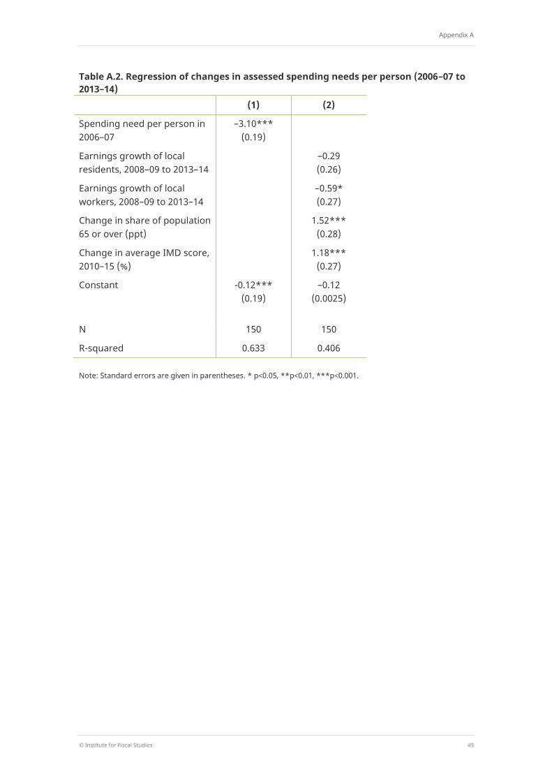
Appendix A
© Institute for Fiscal Studies 45
Table A.2. Regression of changes in assessed spending needs per person (2006–07 to 2013–14)
(1) (2)
Spending need per person in 2006–07
–3.10*** (0.19)
Earnings growth of local residents, 2008–09 to 2013–14
–0.29 (0.26)
Earnings growth of local workers, 2008–09 to 2013–14
–0.59* (0.27)
Change in share of population 65 or over (ppt)
1.52*** (0.28)
Change in average IMD score, 2010–15 (%)
1.18*** (0.27)
Constant -0.12*** (0.19)
–0.12 (0.0025)
N 150 150
R-squared 0.633 0.406
Note: Standard errors are given in parentheses. * p<0.05, **p<0.01, ***p<0.001.
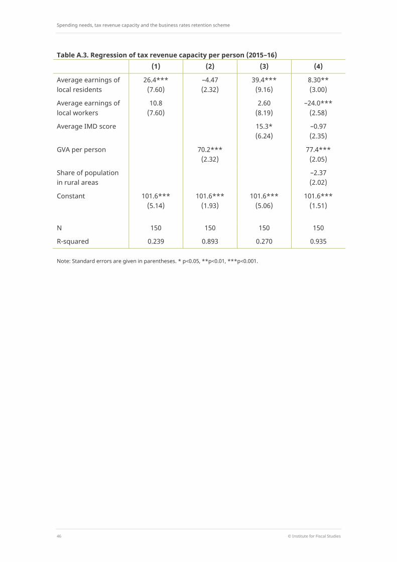
Spending needs, tax revenue capacity and the business rates retention scheme
46 © Institute for Fiscal Studies
Table A.3. Regression of tax revenue capacity per person (2015–16) (1) (2) (3) (4)
Average earnings of local residents
26.4*** (7.60)
–4.47 (2.32)
39.4*** (9.16)
8.30** (3.00)
Average earnings of local workers
10.8 (7.60)
2.60 (8.19)
–24.0*** (2.58)
Average IMD score 15.3* (6.24)
–0.97 (2.35)
GVA per person 70.2*** (2.32)
77.4*** (2.05)
Share of population in rural areas
–2.37 (2.02)
Constant 101.6*** (5.14)
101.6*** (1.93)
101.6*** (5.06)
101.6*** (1.51)
N 150 150 150 150
R-squared 0.239 0.893 0.270 0.935
Note: Standard errors are given in parentheses. * p<0.05, **p<0.01, ***p<0.001.

References
© Institute for Fiscal Studies 47
References Amin-Smith, N., Choo, M., Glover, J., Goldsworthy, J., Jones, N., Lucas, L. and Phillips, D. (2017), ‘The local vantage: how views of local government finance vary across councils’, IFS Report 131, https://www.ifs.org.uk/uploads/publications/comms/R131.pdf.
Amin-Smith, N., Eiser, D., Phillips, D., Simpson, P. and Trickey, M. (2016), ‘A time of revolution? British local government finance in the 2010s’, IFS Report 121, https://www.ifs.org.uk/uploads/publications/comms/R121.pdf.
Centre for Cities (2017), ‘Business rates: maximising the growth incentive across the country’, http://www.centreforcities.org/wp-content/uploads/2017/12/17-12-07-Business-rates-maximising-the-growth-incentive-across-the-country.pdf.
Department for Communities and Local Government (2012), ‘Business rates retention: policy statement’, https://www.gov.uk/government/uploads/system/uploads/attachment_data/file/14939/Business_rates_retention_policy_statement.pdf.
Department for Communities and Local Government (2017a), ‘100% business rates retention: further consultation on the design of the reformed system’, https://www.gov.uk/government/consultations/100-business-rates-retention-further-consultation-on-the-design-of-the-reformed-system.
Department for Communities and Local Government (2017b), ‘Provisional local government finance settlement 2018 to 2019: statement’, https://www.gov.uk/government/speeches/provisional-local-government-finance-settlement-2018-to-2019-statement.
Department for Communities and Local Government (2017c), ‘100% business rates retention: further consultation on the design of the reformed system’, https://www.gov.uk/government/uploads/system/uploads/attachment_data/file/592368/100__Business_Rates_Retention_-_Further_Consultation.pdf.
Local Government Association (2018), ‘The 2018/19 Provisional Local Government Finance Settlement’, https://www.local.gov.uk/sites/default/files/documents/The%202018-19%20Provisional%20Local%20Government%20Finance%20Settlement%20-%20response.pdf.
Phillips, D. and Simpson, P. (2017), ‘National standards, local risks: the geography of local authority funded social care, 2009–10 to 2015–16’, IFS Report 128, https://www.ifs.org.uk/uploads/publications/comms/R128.pdf.

Spending needs, tax revenue capacity and the business rates retention scheme
48 © Institute for Fiscal Studies
Data references Chartered Institute of Public Finance and Accountancy (CIPFA) (2016), Finance and general estimates: 2006–07 to 2015–16. https://www.cipfastats.net/general/financegeneral/ (accessed 10 April 2017).
Department for Communities and Local Government (2011), English indices of deprivation 2010. https://www.gov.uk/government/statistics/english-indices-of-deprivation-2010 (accessed 14 March 2017).
Department for Communities and Local Government (2013a), Calculation of 2013–14 Formula Funding. http://webarchive.nationalarchives.gov.uk/20140505105851/http://www.local.communities.gov.uk/finance/1314/CalcFFs.pdf (accessed 8 November 2017); formulae and data for earlier years provided directly by the Department for Communities and Local Government.
Department for Communities and Local Government (2013b), NNDR3 local authority data: 2006 to 2007 – 2013 to 2014. https://www.gov.uk/government/statistical-data-sets/national-non-domestic-rates-local-authority-level-data (accessed 22 August 2016).
Department for Communities and Local Government (2015), English indices of deprivation 2015. https://www.gov.uk/government/statistics/english-indices-of-deprivation-2015 (accessed 13 March 2017).
Department for Transport (2013), Road lengths in Great Britain, 2013 – Major: Principal Roads. https://www.gov.uk/government/collections/road-network-size-and-condition (accessed 20 July 2017).
Office for National Statistics (2011), Census 2011, ‘Rural including hub towns population’ and ‘Total population’. https://www.nomisweb.co.uk/census/2011 (accessed 12 June 2017).
Office for National Statistics (2013a), Annual Survey of Hours and Earnings – resident analysis, full time workers, median, weekly pay – gross. https://www.nomisweb.co.uk/datasets/ashe (accessed 12 June 2017).
Office for National Statistics (2013b), Annual Survey of Hours and Earnings – workplace analysis, full time workers, median, weekly pay – gross. https://www.nomisweb.co.uk/datasets/ashe (accessed 12 June 2017).
Office for National Statistics (2015a), Population estimates – local authority based by year of age. https://www.nomisweb.co.uk/default.asp (accessed 22 February 2017).
Office for National Statistics (2015b), Annual Population Survey – workplace analysis. https://www.nomisweb.co.uk/datasets/apsnew (accessed 26 June 2017).

Data references
© Institute for Fiscal Studies 49
Office for National Statistics (2016), Regional gross value added (income approach) by local authority in the UK. https://www.ons.gov.uk/economy/grossvalueaddedgva/datasets/regionalgvaibylocalauthorityintheuk (accessed 12 June 2017).
Valuation Office Agency (2017), Non-domestic rating: change in rateable value of rating lists, England and Wales, 2017 Revaluation. https://www.gov.uk/government/statistics/non-domestic-rating-change-in-rateable-value-of-rating-lists-england-and-wales-2017-revaluation (accessed 15 November 2017).