sph simulation within the openfoam framework · outlineintroductionmotivationsmoothed particle...
TRANSCRIPT

Outline Introduction Motivation Smoothed Particle Hydrodynamics Numerical Examples References
SPH simulation within the OpenFOAMframework
Pankaj Kumar, Qing Yang, Van Jones, and Leigh McCue
Aerospace and Ocean Engineering
Virginia Polytechnic Institute and State University
June 14, 2011

Outline Introduction Motivation Smoothed Particle Hydrodynamics Numerical Examples References
Introduction
Motivation
Smoothed Particle Hydrodynamics
Numerical Examples

Outline Introduction Motivation Smoothed Particle Hydrodynamics Numerical Examples References
Outline
Introduction
Motivation
Smoothed Particle Hydrodynamics
Numerical Examples

Outline Introduction Motivation Smoothed Particle Hydrodynamics Numerical Examples References
Grid Based Numerical Schemes
Reference [2]
Reference [1]

Outline Introduction Motivation Smoothed Particle Hydrodynamics Numerical Examples References
Outline
Introduction
Motivation
Smoothed Particle Hydrodynamics
Numerical Examples

Outline Introduction Motivation Smoothed Particle Hydrodynamics Numerical Examples References
Grid Based Numerical Methods

Outline Introduction Motivation Smoothed Particle Hydrodynamics Numerical Examples References
Smoothed Particle Hydrodynamics (SPH)
Outline Introduction Motivation Smoothed Particle Hydrodynamics Numerical Examples References
Outline
Introduction
Motivation
Smoothed Particle Hydrodynamics
Numerical Examples

Outline Introduction Motivation Smoothed Particle Hydrodynamics Numerical Examples References
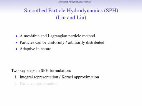
Smoothed Particle Hydrodynamics (SPH)(Liu and Liu)
• A meshfree and Lagrangian particle method• Particles can be uniformly / arbitrarily distributed• Adaptive in nature
Two key steps in SPH formulation:
1. Integral representation / Kernel approximation
2. Particle approximation

Outline Introduction Motivation Smoothed Particle Hydrodynamics Numerical Examples References
Smoothed Particle Hydrodynamics (SPH)(Liu and Liu)
• A meshfree and Lagrangian particle method• Particles can be uniformly / arbitrarily distributed• Adaptive in nature
Two key steps in SPH formulation:
1. Integral representation / Kernel approximation
2. Particle approximation

Outline Introduction Motivation Smoothed Particle Hydrodynamics Numerical Examples References
Integral Representation / Kernel Approximation(Liu and Liu)
f (x) =
∫Ω
f (x′)δ(x− x′)dx′
Ω is the volume of the domain and prime denotes neighboringvariables.δ(x− x′) is the Dirac delta function:
δ(x− x′) =
1 if x = x′
0 if x 6= x′
Replacing the dirac delta function with a smoothing function, in SPHconvention called kernel function, W(x− x′, h)
f (x) =
∫Ω
f (x′)W(x−x′, h)dx′ ∇f (x) =
∫Ω
[∇f (x′)
]W(x−x′, h)dx′

Outline Introduction Motivation Smoothed Particle Hydrodynamics Numerical Examples References
Kernel Function(Liu and Liu)
1. Even function2. Normalization condition / unity condition:∫
ΩW(x− x′, h)dx′ = 1
3. Delta function property:
limh→0
W(x− x′, h) = δ(x− x′)
4. W(x− x′, h) ≥ 0, monotonically decreasing5. Compact condition:
W(x− x′, h) = 0 when |x− x′| > kh

Outline Introduction Motivation Smoothed Particle Hydrodynamics Numerical Examples References
Particle Approximation(Liu and Liu)
To approximate the continuous integral representations as discretizedform of summation over all the particles in the support domain.
f (xi) ≈N∑
j=1
mj
ρjf (xj)W(xi − xj, h)
∇ · f (xi) ≈ −N∑
j=1
mj
ρjf (xj)∇W(xi − xj, h)

Outline Introduction Motivation Smoothed Particle Hydrodynamics Numerical Examples References
Governing Equations of Fluid Dynamics(Liu and Liu)
Conservation of Mass
DρDt
= −ρ∇ ·~v
SPH formulation of Conservation of Mass
Dρi
Dt= ρi
N∑j=1
mj
ρjvβij∂Wij
∂xβi

Outline Introduction Motivation Smoothed Particle Hydrodynamics Numerical Examples References
Governing Equations of Fluid Dynamics(Liu and Liu)
Conservation of Mass
DρDt
= −ρ∇ ·~v
SPH formulation of Conservation of Mass
Dρi
Dt= ρi
N∑j=1
mj
ρjvβij∂Wij
∂xβi

Outline Introduction Motivation Smoothed Particle Hydrodynamics Numerical Examples References
Governing Equations of Fluid Dynamics(Liu and Liu)
Conservation of Momentum
Dvα
Dt= −1
ρ
∂σαβ
∂xβ
SPH formulation of Conservation of Momentum
DvαiDt
=
N∑j=1
mjσαβi + σαβj
ρiρj
∂Wij
∂xβi

Outline Introduction Motivation Smoothed Particle Hydrodynamics Numerical Examples References
Governing Equations of Fluid Dynamics(Liu and Liu)
Conservation of Momentum
Dvα
Dt= −1
ρ
∂σαβ
∂xβ
SPH formulation of Conservation of Momentum
DvαiDt
=
N∑j=1
mjσαβi + σαβj
ρiρj
∂Wij
∂xβi
Outline Introduction Motivation Smoothed Particle Hydrodynamics Numerical Examples References
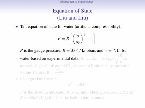
Equation of State(Liu and Liu)
• Tait equation of state for water (artificial compressibility):
P = B[(
ρ
ρ0
)γ
− 1]
P is the gauge pressure, B = 3.047 kilobars and γ = 7.15 for
water based on experimental data. Since ∆t = CFLp/√
Bρ
, a
numerical speed of sound Cs0 chosen to limit density variationwithin 1% and B =
Cs20ρ0γ
• Ideal gas law for air:P = ρRT
P is the absolute pressure, R is the individual gas constant, for airR = 286.9(J/kgK), T is the Kelvin temperature.

Outline Introduction Motivation Smoothed Particle Hydrodynamics Numerical Examples References
Boundary ConditionMonaghan-type Boundary Condition (Monaghan): The force per unit massacting from a boundary particle to a fluid particle within its neighboringdomain is:
~f = ~nR(η)P(ξ)
~n: Normal of the boundary particle; η: Normal distance from the fluidparticle to the boundary particle; ξ: the distance between the fluid particleand the boundary particle projected on the tangent of the boundary particle.
R(η) = A1− q√
q
q = η2∆p , A = 1
h
(0.01ca
2 + β caVab nb). ∆p: the boundary particle spacing,
c is the numerical speed of sound of particles, and:
β =
0 if Vab > 01 if Vab < 0
P(ξ) =12
(1 + cos
(πξ
∆p
))

Outline Introduction Motivation Smoothed Particle Hydrodynamics Numerical Examples References
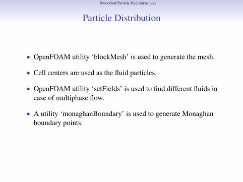
Particle Distribution
• OpenFOAM utility ‘blockMesh’ is used to generate the mesh.
• Cell centers are used as the fluid particles.
• OpenFOAM utility ‘setFields’ is used to find different fluids incase of multiphase flow.
• A utility ‘monaghanBoundary’ is used to generate Monaghanboundary points.

Outline Introduction Motivation Smoothed Particle Hydrodynamics Numerical Examples References
Particle Distribution
• OpenFOAM utility ‘blockMesh’ is used to generate the mesh.
• Cell centers are used as the fluid particles.
• OpenFOAM utility ‘setFields’ is used to find different fluids incase of multiphase flow.
• A utility ‘monaghanBoundary’ is used to generate Monaghanboundary points.
Outline Introduction Motivation Smoothed Particle Hydrodynamics Numerical Examples References
Outline
Introduction
Motivation
Smoothed Particle Hydrodynamics
Numerical Examples

Outline Introduction Motivation Smoothed Particle Hydrodynamics Numerical Examples References
Dam Collapse with Free Surface
Dam-break problem and impact against a rigid obstetrical and walls.Geometrical parameters:H = 0.1m, L/H = 1, D/H = 1.5, d/H = 2, hb/H = 0.4, lb/H = 0.2,b/H = 1.4, Cs = 10
√2gH, γ = 7.0, B = 1
γρC2s

Outline Introduction Motivation Smoothed Particle Hydrodynamics Numerical Examples References
Dam Collapse with Free Surface
t√
(g/H) = 0.0
t√
(g/H) = 2.97
t√
(g/H) = 1.98
t√
(g/H) = 3.96

Outline Introduction Motivation Smoothed Particle Hydrodynamics Numerical Examples References
Dam Collapse: Multi Phase(Colagrossi and Landrini)
Dam-break problem and impact against a rigid walls.Geometrical parameters:H = 0.6m, L/H = 2, D/H = 3, d/H = 5.366, Nx = 391, Ny = 2885,CX = 10.9
√2gH, γX = 7.0, BX = 17.4ρgH, CY = 155
√2gH,
γY = 7.0, BY = BX ,

Outline Introduction Motivation Smoothed Particle Hydrodynamics Numerical Examples References
Dam Collapse: Multi Phase using SPH
t√
(g/H) = 0.00
t√
(g/H) = 1.62
t√
(g/H) = 0.81
t√
(g/H) = 2.63

Outline Introduction Motivation Smoothed Particle Hydrodynamics Numerical Examples References
Dam Collapse: Multi Phase using RANS
t√
(g/H) = 0.00
t√
(g/H) = 1.62
t√
(g/H) = 0.81
t√
(g/H) = 2.63

Outline Introduction Motivation Smoothed Particle Hydrodynamics Numerical Examples References
Dam Collapse: Multi PhaseTime Evolution of Water-Front Toe
0 0.5 1 1.5 2 2.52
2.5
3
3.5
4
4.5
5
5.5
x front
/H
t(g/H)0.5
SPHRAS
Outline Introduction Motivation Smoothed Particle Hydrodynamics Numerical Examples References
Conclusion
• SPH solver is developed into the OpenFOAM framework.
• Direct comparison of results for meshfree and grid basedmethods are possible into the OpenFOAM framework.
• It is possible to use SPH and RANS together to capitalize on thebest of both using OpenFOAM framework.

Outline Introduction Motivation Smoothed Particle Hydrodynamics Numerical Examples References
Future Work
• To develop a utility to generate a temporary boundary particlesalong the fluid surface to bring the system into equilibrium attime t = 0.
• To develop a utility to generate ghost particles for SPHsimulation.
• To develop a solver utilizing the benefits of SPH and RANStogether.

Outline Introduction Motivation Smoothed Particle Hydrodynamics Numerical Examples References
References
[1] URL http://www.arl.hpc.mil/Publications/eLink_Fall05/cover.html.
[2] URL http://dspace.mit.edu/bitstream/handle/1721.1/36385/16-21Spring-2003/OcwWeb/Aeronautics-and-Astronautics/16-21Techniques-of-Structural-Analysis-and-DesignSpring2003/CourseHome/index.htm.
[3] Andrea Colagrossi and Maurizio Landrini. Numerical simulation of interfacial flows by smoothed particle hydrodynamics.Journal of Computational Physics, 191:448–475, 2003.
[4] G. R. Liu and M. B. Liu. Smoothed particle hydrodynamics: a meshfree particle method. World Scientific, 2003.
[5] J. J. Monaghan. Simulating free surface flows with sph. Journal of Computational Physics, 110:399–406, 1992.