Spherical Microphone Array Processing in Python

with the sound field analysis-py Toolbox

Christoph Hohnerlein1, Jens Ahrens21Quality & Usability Lab, Technische Universitat Berlin, Deutschland, Email: christoph.hohnerlein@qu.tu-berlin.de2Division of Applied Acoustics, Chalmers University of Technology, Sweden, Email: jens.ahrens@chalmers.se

Abstract

The sound field analysis-py toolbox started as a Pythonport of SOFiA toolbox1 by Benjamin Bernschutz et al.[1], which performs the analysis and processing of datacaptured with spherical microphone arrays. SOFiA iswritten for Matlab with several externals in C/C++ andpublished under the GNU GPLv3 license.The current implementation deals with impulse responsesand headphone playback – frame-based processing, whichwould allow real-time manipulation, is subject to ongoingwork. Furthermore, we are working towards interfacingsound field analysis-py with other existing Python au-dio processing tools, such as the sound field synthesis-pytoolbox [2], to leverage community efforts towards base-line implementations and reproducible research.The sound field analysis-py toolbox is available onGitHub2.

Introduction

Spherical microphones (such as the Eigenmike3) as wellas scanning/sequential arrays (such as the VariSphear4)can be used to record multi-point room impulse re-sponses. Such a set can then be used to retroactivelyapply that room’s reverberation to a signal, similarly totraditional Room Impulse Responses (RIRs). But in con-trast to RIRs, array recordings theoretically allow for afully dynamic reproduction of the rooms response, onlylimited by the spatial resolution of the array.Figure 1 shows two possible workflows: A multi-pointroom IR can either be combined with a set of HRTFsto recreate a virtual scene binaurally or used to gener-ate the corresponding driving functions of a loudspeakerbased sound field synthesis approach, as for example pre-sented in [3]. Apart from capturing impulse responses,spherical microphone arrays also allow for storing andtransmitting of full dynamic sound scenes including allspatial information.

A spherical harmonics expansion of the captured soundfield has shown to be a convenient representation asthis finite discrete set of signals can represent a con-tinuous spherical space. Furthermore, rotations can beperformed elegantly, which is very important for head-tracked binaural playback.

1http://audiogroup.web.th-koeln.de/SOFiA_wiki/WELCOME.

html2https://github.com/QULab/sound_field_analysis-py/

3https://www.mhacoustics.com/products

4http://audiogroup.web.th-koeln.de/varisphear.html

Therefore, most of the work in this package concernstransformations and processing in the spherical harmon-ics space. Unfortunately, the larger theoretical back-ground is out of scope for the paper at hand. As a portof the SOFiA Toolbox [1], our package implements func-tions covered in the corresponding thesis [4], and buildson extended literature such as [5] and [6].

Example workflow

Converting the time domain data into spatial coeffi-cients comprises two steps: First, a standard FourierTransform process.FFT() is applied, followed by eitherthe explicit (if the quadrature is appropriate) or least-squares spatial Fourier transform (process.spatFT() orprocess.spatFT LSF()). Furthermore, it is useful topre-calculate the radial filters that effectively undo theeffects of the microphone array due to its size, trans-ducer type and scattering body (if there is one) usinggen.radial filter fullspec().

Now, the coefficients can be manipulated (for exampleresampled, rotated, weighted) and visualized. Further-more, when the spherical harmonics expansion of a set ofHRTFs is available, the two can be combined by means ofconvolution in the spherical harmonics domain (as shownin [7] and [8]):

Sl,r =∞∑n=0

n∑m=−n

dnPnmHnm , (1)

where dn are the radial filters, Pnm the complex conju-gate of the sound field coefficients and Hnm the HRTFcoefficients.Applying the inverse of the two step transformation(process.ispatFT() and process.iFFT()) to go backto time domain yields a pair of impulse responses thatrepresent the ear signals of a human listener that is ex-posed to the sound field that was captured by the micro-phone array. This process can be performed for differentvirtual head orientations and the data can then be ex-ported for binaural rendering using the SoundScapeRen-derer using io.write SSR IRs().

Some examples are available in the examples folder onGitHub.

Modules

The sound field analysis-py package contains several sub-modules; the most important ones gen, process, plotand io are briefly introduced in the following.

Figure 1: The sound field captured by a spherical microphone array can be combined with an HRTF dataset by means ofconvolution in the spherical harmonics domain to produce dynamic binaural room simulations or added to a speaker-basedsound field reproduction setup, such as Wave Field Synthesis [3].

Generators

The gen package contains all routines that generate databased only on meta data.

Sound fields

There are two functions that directly return the coeffi-cients of a synthesized sound field: ideal wave() andsampled wave(). Both simply need a description ofthe desired sound field, such as the configuration of thesimulated microphone array, type and direction of theimpinging wave.

Quadratures

Gauss and Lebedev quadratures (both explicitly inte-grable) can be generated using gen.gauss grid() andgen.lebedev(). For the Lebedev grid, stable ordersup to N = 11 (corresponding to a degrees of L ∈[6, 14, 26, 38, 50, 74, 86, 110, 146, 170, 194]) can be satis-fied. It is based on Richard P. Muller’s Python imple-mentation5 of [9].

Radial Filters

Radial filters for three different configurations (opensphere, rigid sphere, dual sphere) using 2 different trans-ducer types (omni and cardiod) are implemented, exclud-ing the dual cardioid configuration.

Processing

The processing submodule contains functions that trans-form existing data.

Fourier Transform

The process.FFT and process.iFFT function rely onNumpy’s fft.rfft routine to perform time↔ frequencytransformations. All frequency-domain signals are ex-pected to be one-sided and all time-domain signals to bereal.

5https://github.com/gabrielelanaro/pyquante/blob/

master/Data/lebedev_write.py

Convolution

Convolution is either performed in the frequency domain(fast convolution) using scipy.signal.fftconvolve()

or in the time domain using numpy.convolve(). Unlessexplicitly set, the mode is automatically set to the fasterone (switching from time domain to fast convolution if∀N > 500).

Spatial Fourier Transform

Generally, the spherical harmonics coefficients Pnm(ω)of order n, degree m and frequency ω that correspondto a frequency-domain function F (ω,Ω) at positions Ω isderived through the expansion integral over a continuousunit sphere S:

Pnm(ω) =

∫S

F (ω,Ω)Y mn (Ω)dΩ , (2)

with Y mn (Ω) as the complex conjugate spherical harmonicbasis functions. Because the unit sphere is not continu-ously measured with a real microphone array but insteadsampled at discrete points Ωi, the spherical harmonicscoefficients can be determined by two different methods.

Firstly, Eq. 2 can be approximated in discrete spaceover an integrable spherical quadrature, as implementedin process.spatFT():

Pnm(ω) =〈(4πwiYmn (Ωi)), F (ω,Ωi)〉 (3)

where 〈 , 〉 denotes the inner product; Y mn (Ωi) the com-plex conjugate of the spherical harmonic basis functionsat the discrete positions Ωi; wi the quadrature weights as-sociated with each position and F (ω,Ωi) the correspond-ing frequency-domain signals.

As an alternative, a least-square fit of spherical har-monic coefficients on the data is implemented inprocess.spatFT LSF(), which solves:

argminPnm(ω)

||〈Y mn (Ωi), Pnm(ω)〉 − F (ω,Ωi)||2 (4)

for Pnm(ω) in the least-square sense, where || · ||2 is theL2 norm.

The inverse spatial Fourier Transformprocess.ispatFT() is implemented as:

F (ω,Ωi) =〈Y mn (Ωi), Pnm(ω)〉 (5)

Plane Wave Decomposition

Plane wave decomposition of directions Ωi is computedas:

D(ω,Ωi) = 〈Y mn (Ωi), dn(kr)Pnm(ω)〉 (6)

where Y mn (Ωi) are the spherical basis functions of direc-tions Ωi, dn(kr) are the radial filters at wavenumber k &radius r and Pnm(ω) are the spherical field coefficients.

Rotation

Currently, only rotation around the vertical axis has beenimplemented, which is the most important rotation whenhead-tracking is considered. It is expressed as a complexphase at reconstruction:

F (ω) =

∞∑n=0

n∑m=−n

Pnm(ω) e−im∆α︸ ︷︷ ︸∆α rotation

dn(kr)Y mn (Ωi) (7)

The implementation of arbitrary rotations is subject toon-going work.

Spherical math utilities

The sph subpackage contains mathematical expressionsthat are needed when dealing with spherical arrays.Specifically, this includes various Bessel functions, theirspherical expression and their respective derivatives:

– Bessel Jn(x), jn(x), j′n(x) (normal, spherical, spher-ical derivative)besselj | spbessel | dspbessel(n, z)

– Neumann Yn(x), ... (Weber / Bessel 2nd kind)neumann(n, z) | ...

– Hankel H(1)/(2)n (x), ... (1st / 2nd kind)

hankel1(n, z) | ...

hankel2(n, z) | ...

Furthermore, spherical harmonic basis functionsY mn (ϕ, θ) up to order Nmax = 85 of several types (seeEq. 8 – 10) can be generated on an arbitrary grids usingthe sph.sph harm() function.

Plotting

Each processing stage can be evaluated via various waysof plotting data, which is internally offloaded to thePlotly.py package. This produces highly portable, in-teractive plots that render in the browser using the D3.jslibrary.

2D

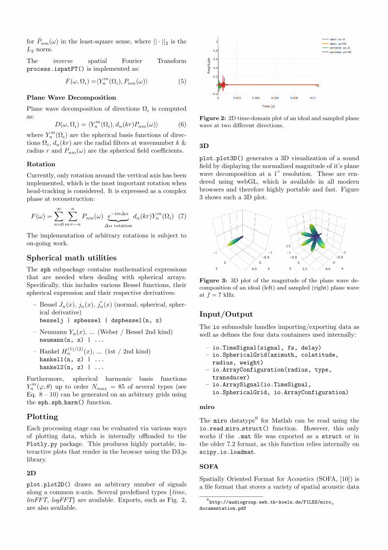
plot.plot2D() draws an arbitrary number of signalsalong a common x-axis. Several predefined types time,linFFT, logFFT are available. Exports, such as Fig. 2,are also available.

Figure 2: 2D time-domain plot of an ideal and sampled planewave at two different directions.

3D

plot.plot3D() generates a 3D visualization of a soundfield by displaying the normalized magnitude of it’s planewave decomposition at a 1 resolution. These are ren-dered using webGL, which is available in all modernbrowsers and therefore highly portable and fast. Figure3 shows such a 3D plot.

Figure 3: 3D plot of the magnitude of the plane wave de-composition of an ideal (left) and sampled (right) plane waveat f = 7 kHz.

Input/Output

The io submodule handles importing/exporting data aswell as defines the four data containers used internally:

– io.TimeSignal(signal, fs, delay)– io.SphericalGrid(azimuth, colatitude,

radius, weight)– io.ArrayConfiguration(radius, type,

transducer)– io.ArraySignal(io.TimeSignal,

io.SphericalGrid, io.ArrayConfiguration)

miro

The miro datatype6 for Matlab can be read using theio.read miro struct() function. However, this onlyworks if the .mat file was exported as a struct or inthe older 7.2 format, as this function relies internally onscipy.io.loadmat.

SOFA

Spatially Oriented Format for Acoustics (SOFA, [10]) isa file format that stores a variety of spatial acoustic data

6http://audiogroup.web.th-koeln.de/FILES/miro_

documentation.pdf

such as HRTFs, BRIRs or array recordings and is stan-dardized as AES69-20157. It is based on the efficientHDF5 format and currently only provides a C++ andMatlab API. It can however be read into Python usingthe netCDF4 package. A small tutorial was made avail-able as an example on GitHub8.

SoundScapeRenderer

The function io.write SSR IRs() exports impulse re-sponses into a .wav file compatible with the binauralrenderer of the SSR which allows for dynamic evaluationwith head-tracking [11].

Conventions

Signal data structure

Python/Numpy’s arrays can be dimensionless, contraryto e.g. Matlab. Internally, such an array is assumed tobe a single signal. If more than one signal are combinedinto a [M x N] matrix, it is treated as M signals oflength N (row-major).

Spherical Harmonics

In order to be compatible with the SH definitions mostcommonly found in the literature, three different spheri-cal harmonic basis functions are implemented: Complex(Eq. 8), real (Eq. 9) and so called ”legacy” (Eq. 10,without Condon–Shortley phase). The complex defini-tion is used internally.

N(m,n, θ) =

√2n+ 1

4π

(n−m)!

(n+m)!Pmn (cos θ)

Y mn (ϕ, θ) = (−1)mN(|m|, n, θ) · eimϕ (8)

Y mn (ϕ, θ) = (−1)mN(|m|, n, θ) ·

√

2 cos(mϕ), m > 0

1, m = 0√2 sin(mϕ), m < 0

(9)

Y mn (ϕ, θ) =N(m,n, θ) · eimϕ (10)

Future Development

Currently, all implementations are carried out in terms ofimpulse responses. This means that sound field analysis-py reads room impulse responses captured by a spher-ical microphone array and produces ear impulse re-sponses. Ways of applying the same processing to signalstreams in a frame-based fashion are investigated, whichwould allow for real-time processing. This would likelybe accomplished by interfacing with sounddevice

9 andjackclient

10 packages. This would allow for fast evalu-ation of sound fields directly from Python.

7http://www.aes.org/publications/standards/search.cfm?

docID=998https://github.com/QULab/sound_field_analysis-

py/blob/master/examples/Exp3_Import_SOFA.ipynb9https://python-sounddevice.readthedocs.io/

10https://jackclient-python.readthedocs.io/

Acknowledgments

We would like to thank Benjamin Bernschutz for hiscontinued support, as well as Matthias Geier for themany fruitful discussions.

References

[1] Benjamin Bernschutz, Christoph Porschmann,Sascha Spors, and Stefan Weinzierl. SOFiA soundfield analysis toolbox. In Proceedings of the Inter-national Conference on Spatial Audio (ICSA), pages7–15, 2011.

[2] Hagen Wierstorf and Sascha Spors. Sound fieldsynthesis toolbox. In Audio Engineering SocietyConvention 132. Audio Engineering Society, 2012.http://sfstoolbox.org.

[3] Jens Ahrens and Sascha Spors. Wave field synthesisof a sound field described by spherical harmonicsexpansion coefficients. The Journal of the AcousticalSociety of America, 131(3):2190–2199, 2012.

[4] Benjamin Bernschutz. Microphone arrays and soundfield decomposition for dynamic binaural recording.PhD thesis, Technische Universitat Berlin, 2016.https://doi.org/10.14279/depositonce-5082.

[5] Jens Ahrens. Analytic Methods of Sound Field Syn-thesis. Springer Berlin Heidelberg, Berlin, Heidel-berg, 2012. http://www.soundfieldsynthesis.

org.

[6] Boaz Rafaely. Fundamentals of spherical array pro-cessing, volume 8. Springer, 2015.

[7] Amir Avni, Jens Ahrens, Matthias Geier, SaschaSpors, Hagen Wierstorf, and Boaz Rafaely. Spa-tial perception of sound fields recorded by sphericalmicrophone arrays with varying spatial resolution.The Journal of the Acoustical Society of America,133(5):2711–2721, 2013.

[8] Carl Andersson. Headphone auralization of acousticspaces recorded with spherical microphone arrays.Master’s thesis, Chalmers University of Technology,2017.

[9] V.I. Lebedev and D.N. Laikov. A quadrature for-mula for the sphere of the 131st algebraic order of ac-curacy. In Doklady. Mathematics, volume 59, pages477–481. MAIK Nauka/Interperiodica, 1999.

[10] Piotr Majdak et al. Spatially oriented format foracoustics: A data exchange format representinghead-related transfer functions. In Audio Engineer-ing Society Convention 134. Audio Engineering So-ciety, 2013. https://www.sofaconventions.org/.

[11] Jens Ahrens, Matthias Geier, and Sascha Spors.The soundscape renderer: A unified spatial au-dio reproduction framework for arbitrary renderingmethods. In Audio Engineering Society Conven-tion 124. Audio Engineering Society, 2008. http:

//spatialaudio.net/ssr/.