spherical minimax location problem

Computational Optimization and Applications, 18, 311–326, 2001c© 2001 Kluwer Academic Publishers. Manufactured in The Netherlands.

Spherical Minimax Location Problem

P. DAS, N.R. CHAKRABORTI AND P.K. CHAUDHURIDepartment of Mathematics, North Bengal University, Darjeeling, West Bengal 734430, India

Received September 12, 1995; Accepted August 3, 1999

Abstract. This paper presents an algorithm for determining a minimax location to service demand points thatare equally weighted and distributed over a sphere. The norm under consideration is geodesic. The algorithmpresented here is based on enumeration and has a polynomial time complexity.

Keywords: minimax location, Geodesic norm, algorithm

1. Introduction

Spherical location problems typically involve finding the optimal location of a servicefacility among a number of demand points situated on the surface of a sphere (see, e.g.,[1, 2, 4–10, 14–18, 22, 24, and 28]). A number of military, civil and commercial logisticsand location problems are concerned with globally distributed demand points (e.g., [15and 28]). In these problems, the distance metric should span over a sphere and the planardistance approximation may be too crude to be applicable.

This paper considers the spherical minimax location problem that finds the location of aservice facility for which the largest distance to a demand point is minimized. The minimaxspherical problem differs from its planar counterpart (see, e.g., [12, 18, and 29]) in that itsobjective function is nonconvex and nondifferentiable. In a special case where all demandpoints lie on a hemisphere, geometrical algorithms (e.g., [3, 11–13, 19–21, and 25]) for thetwo-dimensional minimax problem using the Euclidean norm can be applied. Recently,Das et al. [4] propose an algorithm for a hemispherical minimax location problem usingcoordinate geometry. In addition, Sarkar and Chaudhuri [24] present an efficient geomet-rical algorithm based on geodesic distance and Litwhiler’s method [15] stereographicallyprojects spherical surfaces bounded by planes on to plane circles so that techniques fortwo and three-dimensional spaces can be used. Given a set of demand points on a sphere,algorithms in [23] and [27] determine whether the points lie on a hemisphere.

When the demand points do not lie on a hemisphere. Drezner and Wesolowsky [10]proposed a steepest descent technique to solve the minimax problem. Recently, Patel [22]proposed another algorithm based on a factored secant update technique. Both algorithmsonly produce local optimal solutions. In theory, one can obtain a global optimal solutionby generating all local solutions. However, to generate all local minima based on differentinitial guesses is difficult, if not impossible, to implement in practice. The procedurepresented here is based on an enumeration technique and determines global optimal solutions

312 DAS, CHAKRABORTI AND CHAUDHURI

in a finite number of steps. When a local minimum is obtained, one uses this informationto obtain the next better solution(s).

Without loss of generality assume that the sphere has a unit radius, since the arc lengthis directly proportional to the radius of the sphere. Let Di (φi , θi ) denote the location on thesurface of a unit sphere of thei -th demand point whereφi andθi represent its latitude andlongitude, respectively, and S denote the set of all demand points. The geodesic distance,αi , between a facility location (φ, θ ) and thei -th demand point is given by (see, e.g., [22and 26])

cosαi = sinφ sinφi + cosφ cosφi cos(θ − θi ) (1)

Thus the location problem on the surface of the sphere can be stated as

min(φ,θ)

{max

iαi}

(2)

For the remainder, Section 2 provides definitions and basic results in spherical trigonom-etry and Section 3 contains the main results. Section 4 proposes an algorithm for thespherical minimax location problem and examines its computational complexity. The nexttwo sections, Sections 5 and 6, discuss the PASCAL implementation of the algorithm andreport of the numerical results for randomly generated problems as well as those in theliterature. Finally, Section 7 concludes the paper.

2. Basic spherical trigonometry

Basic definitions and results from [26] are restated here for convenience.

Definition 2.1. Every plane section of a sphere is a circle. The largest circle which canbe drawn on the surface of a sphere is a circle whose plane passes through the center of thesphere. Such a circle is called agreat circle. All other circles on the surface of the sphereare calledsmall circles.

The above definition leads to the following proposition:

Proposition 2.1. Through any two points on the surface of a sphere, which are not dia-metrically opposite, one and only one great circle can be drawn.

Definition 2.2. Thepolesof a great circle are the extremities of a diameter of the spherethat is perpendicular to the plane of the great circle. This diameter is also known as theaxisof the great circle.

Note that the two poles for a great circle are equidistant from its plane and the centerof the sphere. The poles and axes of small circles are similarly defined. However, sincethe plane of a small circle does not contain the center of the sphere, its two poles are at

SPHERICAL MINIMAX LOCATION PROBLEM 313

a different distance from the plane of the small circle, one is nearer and the other is moredistant. For convenience, refer to them as the nearer and distant poles of a small circle.

Definition 2.3. Let A and B be two points on the surface of a sphere. Then, there is aunique great circle that passes through the two points. Moreover, A and B divide the greatcircle into two arcs. The length of the shorter arc is thedistancebetween A and B or thelength of arc joiningA andB and this distance or length is denoted as

_AB.

Since the sphere has a unit radius, the length of arc AB is simply the angle (measuredin, e.g., radians) between two rays emanating from the center of the sphere, O, one passingthrough A and the other through B.

Definition 2.4. The surface area of a sphere that is bounded by arc segments of three greatcircles is called aspherical triangle.

If the spherical triangle has zero area, i.e., the three arcs intersect at a single point, then itis a degenerate spherical triangle, a case not considered in this paper. Assume as in Article22 in [26] that each side of a spherical triangle is less thanπ . This assumption yields thefollowing proposition:

Proposition 2.2. The sum of any two sides of a spherical triangle is greater than the third.

3. Preliminary concepts and results

The following notation will be used throughout the remainder of the paper:ABC ≡ thespherical anglesubtended from a point B (on the surface of a sphere) by the(shorter) arc AC.1ABC ≡ the plane triangle with vertices at points A,B, and C. Denote the angles of1ABC as<A, <B, <C or,<BAC, <ABC, <ACB.

As in [26], the spherical angle ABC is measured as the angle between two straight linestangential at point B to the two great circles, one passing through A & B and theotherthrough B & C.

The following definitions are necessary for the development of the algorithm.

Definition 3.1. Given three distinct points, A,B, and C on the surface a sphere, II(A,B,C)denotes the unique plane passing through the three points and bisecting the sphere.

Definition 3.2. 03(A,B,C) denotes the circle traced by the plane II(A,B,C) cuttingthrough the sphere.

Generally,03(A,B,C) is expected to be a small circle. However, it is possible that03(A,B,C) is a great circle.

Definition 3.3. Let A and B be two distinct points on the surface of a sphere that are notdiametrically opposite. Denote the mid point of the (shorter) arc AB as the point P. Then,


02(A,B) represents the small circle that goes through points A and B and has its nearerpole located at point P.

Definition 3.4. The length of the great circle arc from any point on the circumference ofa small circle to its nearer pole is called the spherical radius of the small circle.

Definition 3.5. N02(A,B) and N03(A,B,C) denote the surface area of a sphere thatcontains the nearer pole of and is bounded by02(A,B) and03(A,B,C), respectively.

Definition 3.6. R02(A,B) and R03(A,B,C) denote the surface area of a sphere thatcontains the distant pole of and is bounded by02(A,B) and03(A,B,C), respectively.

Below are the results regarding poles of small circles.

Lemma 3.1. Let P be the nearer pole of03(A, B,C), where1ABC is an acute triangle.Let Q(6= P) be any point on N03(A, B,C) and within the spherical triangle ABC. Then,the spherical radius of03(A, B,C) is greater than minimum{ _QA,

_QB,

_QC}.

Proof: In figure 1, O denotes the center of the circle03(A,B,C). Then A1,B1, and C1

are the points on the circumference of the circle that are diametrically opposite of A, B, andC, respectively. Since1ABC is acute, points B and C cannot lie on the same side of theline joining A and A1. The same is true for points C and A and the line joining B and B1,

and points A and B and the line joining C and C1. Let D be any point of the circumferenceof 03(A,B,C), then obviously

minimum{<AOD, <BOD, <COD} < π/2.

Figure 1.


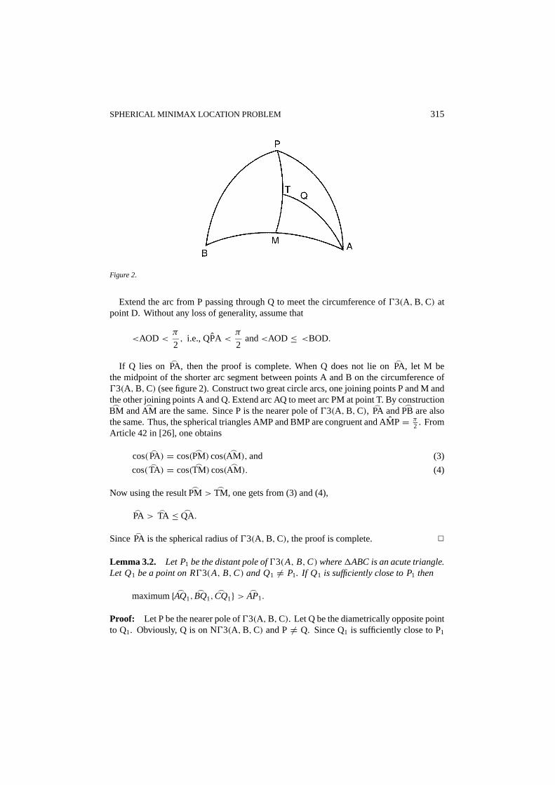
Figure 2.

Extend the arc from P passing through Q to meet the circumference of03(A,B,C) atpoint D. Without any loss of generality, assume that

<AOD <π

2, i.e., QPA<

π

2and<AOD ≤ <BOD.

If Q lies on_PA, then the proof is complete. When Q does not lie on

_PA, let M be

the midpoint of the shorter arc segment between points A and B on the circumference of03(A,B,C) (see figure 2). Construct two great circle arcs, one joining points P and M andthe other joining points A and Q. Extend arc AQ to meet arc PM at point T. By construction_

BM and_

AM are the same. Since P is the nearer pole of03(A,B,C),_PA and

_PB are also

the same. Thus, the spherical triangles AMP and BMP are congruent and AMP= π2 . From

Article 42 in [26], one obtains

cos(_PA) = cos(

_PM) cos(

_AM), and (3)

cos(_TA) = cos(

_TM) cos(

_AM). (4)

Now using the result_

PM>_

TM, one gets from (3) and (4),

_PA>

_TA ≤ _

QA.

Since_PA is the spherical radius of03(A,B,C), the proof is complete. 2

Lemma 3.2. Let P1 be the distant pole of03(A, B,C)where1ABC is an acute triangle.Let Q1 be a point on R03(A, B,C) and Q1 6= P1. If Q1 is sufficiently close to P1 then

maximum{ _AQ1,_

BQ1,_

CQ1} > _AP1.

Proof: Let P be the nearer pole of03(A,B,C). Let Q be the diametrically opposite pointto Q1. Obviously, Q is on N03(A,B,C) and P 6= Q. Since Q1 is sufficiently close to P1


and P is in the spherical triangle ABC, Q must be in the spherical triangle as well. Assumethat

_QA = minimum{ _QA,

_QB,

_QC}.

From Lemma 3.1, it follows that_

QA <_PA. Construct two great circle arcs, one joining A

to P1 and the other joining A to Q1. Since P and Q are diametrically opposite of P1 and Q1,respectively, one finds

_AP+ _

AP1 = π = _AQ+ _

AQ1.

Now_

AQ <_

AP⇒ _AP1 <

_AQ1. This proves Lemma 3.2. 2

If all demand points lie in R03(A,B,C), then Lemma 3.2 shows that every point in asmall neighborhood of P1 has an objective function value that is greater than the one at P1.Thus, P1 is locally optimal.

Lemma 3.3. Let A, B, and C be three points on a unit sphere with<C>π/2. Let P andP1 be respectively the nearer and distant poles of03(A, B,C). Then there exists a pointQ, close to P1 such that

maximum{ _AQ,_

BQ,_

CQ} < _AP1 = _

BP1 = _CP1.

Proof: Recall that (see, e.g., Articles 35 and 37 in [26]).

(a) The angles at the base of an isosceles spherical triangle are equal.(b) If one angle of a spherical triangle is greater than another, the side opposite the greater

angle is greater than the side opposite the lesser angle.

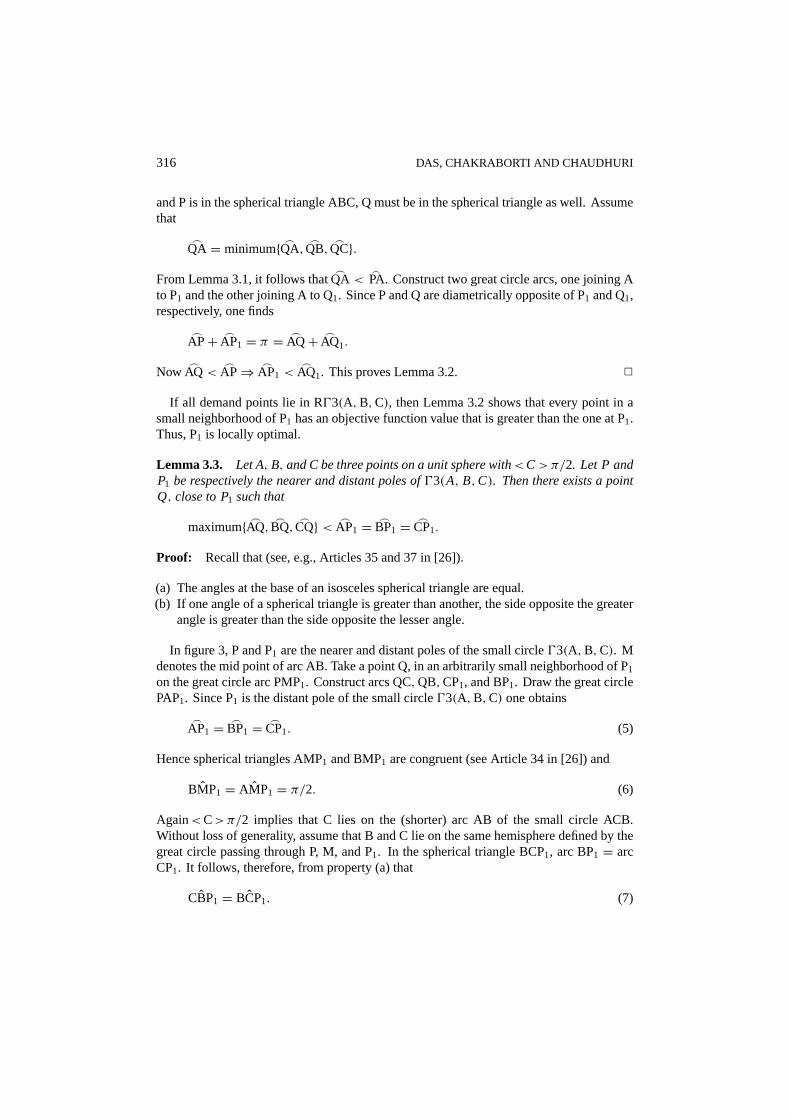
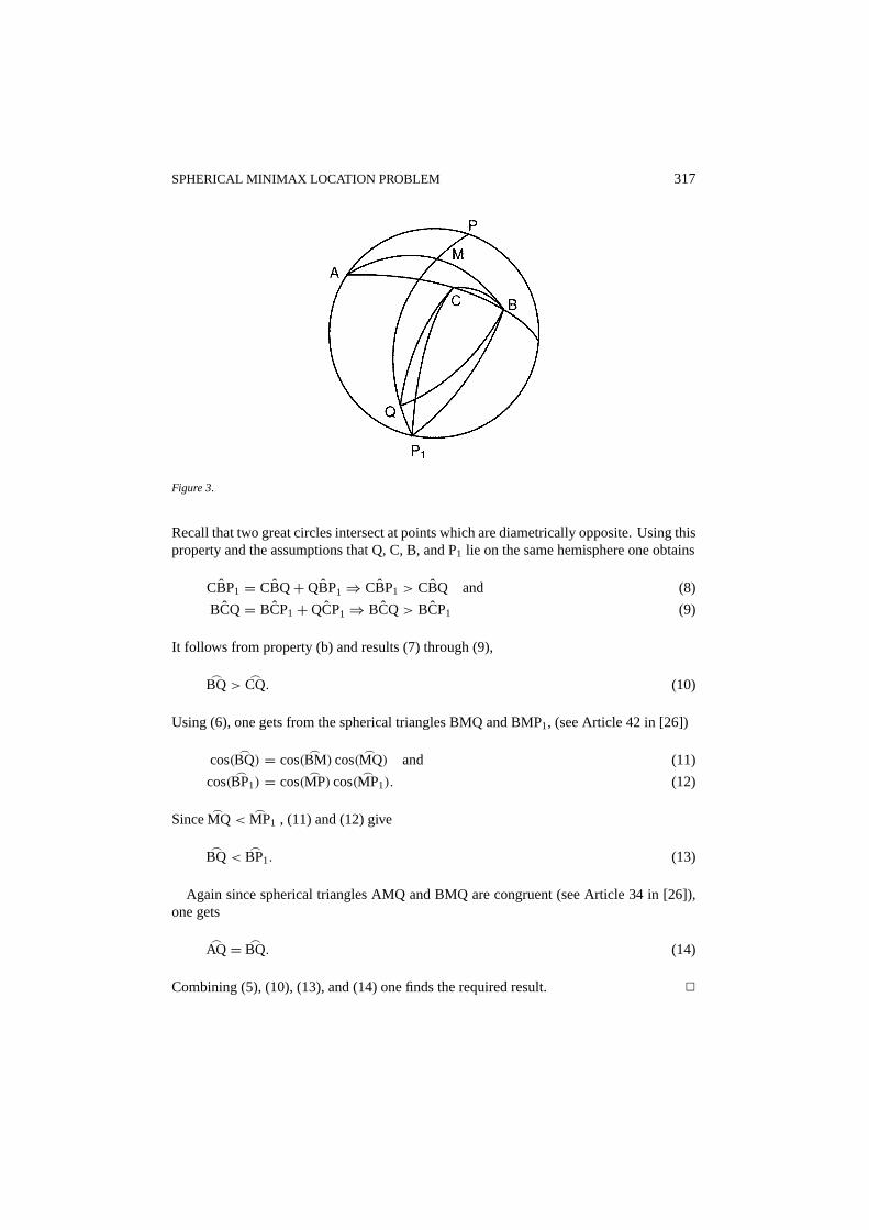
In figure 3, P and P1 are the nearer and distant poles of the small circle03(A,B,C). Mdenotes the mid point of arc AB. Take a point Q, in an arbitrarily small neighborhood of P1

on the great circle arc PMP1. Construct arcs QC,QB,CP1, and BP1. Draw the great circlePAP1. Since P1 is the distant pole of the small circle03(A,B,C) one obtains

_AP1 = _

BP1 = _CP1. (5)

Hence spherical triangles AMP1 and BMP1 are congruent (see Article 34 in [26]) and

BMP1 = AMP1 = π/2. (6)

Again<C>π/2 implies that C lies on the (shorter) arc AB of the small circle ACB.Without loss of generality, assume that B and C lie on the same hemisphere defined by thegreat circle passing through P, M, and P1. In the spherical triangle BCP1, arc BP1 = arcCP1. It follows, therefore, from property (a) that

CBP1 = BCP1. (7)


Figure 3.

Recall that two great circles intersect at points which are diametrically opposite. Using thisproperty and the assumptions that Q, C, B, and P1 lie on the same hemisphere one obtains

CBP1 = CBQ+QBP1⇒ CBP1 > CBQ and (8)

BCQ= BCP1+QCP1⇒ BCQ> BCP1 (9)

It follows from property (b) and results (7) through (9),

_BQ>

_CQ. (10)

Using (6), one gets from the spherical triangles BMQ and BMP1, (see Article 42 in [26])

cos(_

BQ) = cos(_

BM) cos(_

MQ) and (11)

cos(_

BP1) = cos(_

MP) cos(_

MP1). (12)

Since_

MQ <_

MP1 , (11) and (12) give

_BQ<

_BP1. (13)

Again since spherical triangles AMQ and BMQ are congruent (see Article 34 in [26]),one gets

_AQ = _

BQ. (14)

Combining (5), (10), (13), and (14) one finds the required result. 2


Corollary 3.1. 03(A, B,C)may contain demand points other than A, B, and C. Assumethat all other demand points lie in R03(A, B,C) − 03(A, B,C). Then the distant poleof 03(A, B,C) is not a solution of the spherical minimax problem if no triplet of demandpoints on03(A, B,C) forms an acute triangle.

Proof: In this case the demand points on03(A, B,C) lie on an arc of a semicircle. Theresult follows immediately from Lemma 3.3.

Theorem 3.1 addresses the case when all demand points lie in a hemisphere and its prooffollows from Lemmas 2 and 4 in [24]. 2

Theorem 3.1. (i) If 1ABC is an acute triangle and N03(A, B,C) contains all demandpoints then the nearer pole of02(A, B,C) is the unique facility point.

(ii) If N02(A, B) contains all demand points, then the nearer pole of02(A, B) is therequired facility point.

Corollary 3.2. 03(A, B,C)may contain demand points other than A, B, and C. Assumethat all other demand points lie in N03(A, B,C)−03(A, B,C). If all triplets of demandpoints on03(A, B,C) form obtuse triangles, then the nearer pole of03(A, B,C) is notthe required facility point.

Proof: The result follows from Lemma 2 of [24]. 2

When the demand points are distributed over the sphere, Theorem 3.2 characterizes asolution to the global minimax location problem.

Theorem 3.2. If there exists a triplet(A, B, C) of demand points such that(i) 1ABC is acute,

(ii) The center of the sphere and all demand points lie on the same side of5(A, B,C),and

(iii) (A, B, C) generates the plane closest to the center of the sphere, then the distant poleof 03(A, B,C) is the required facility point.

Proof: Lemma 3.3 implies that the triplet of points forming an obtuse triangle cannotyield an optimal solution. Furthermore, it follows from Lemma 3.2 that the distant poleof the small circle defined by a triplet satisfying (i) and (ii) is a local minimum and (iii)implies optimality. 2

That the distant pole of02(A,B) cannot be a minimax location when R02(A,B) containsall the demand points is demonstrated in the following theorem.

Theorem 3.3. If R02(A, B) − 02(A, B) contains all demand points other than A, B,then the distant pole of02(A, B) cannot be a minimax location.


Figure 4.

Proof: In figure 4, P and P1 denote the nearer and distant poles of02(A,B). Draw thegreat circle PAP1B. Construct the great circle arc joining P and P1 through the mid point,M, of the smaller circle arc AB. For any demand point D1(6= A or B),

_Di P1 <

_BP1 = _

AP1.

In particular, there exists a sufficiently smallε > 0 such that

_Di P1 <

_BP1− 2ε. (15)

Let Qi be a point on the arc PMP1 that is sufficiently near P1 so that

_Di Q1 <

_DP1+ ε. (16)

From (15) and (16),

_Di Q1 <

_BP1− ε. (17)

Since spherical triangles APQi , and BPQi , are congruent,

_AQi = _

BQi . (18)

Consider the spherical triangle BP1Qi . Since BP1Qi = π2 , the cosine rule (see Article 42

in [26]) gives

cos(_

BQi ) = cos(_

BP1) cos(_

Qi P1).


Since all demand point are not on a hemisphere,_

BP1 >π2 . Combining this fact with the

assumption that Qi lies on the arc PMP1 and is in theε-neighborhoods of P1 yields,

cos(_

BQi ) > cos(_

BP1).

Hence,

_BQi <

_BP1. (19)

Since limQi−P1

_BQi = _

BP1, there must exist a small neighborhood around P1 such that, ifQi is in this neighborhood, then

_BQi >

_BP1− ε. (20)

Therefore, it follows from (17), (19) and (20) that

_Di Qi <

_BQi <

_BP1. (21)

The results (16) through (20) are not only true for Qi but also for any Q on the arc P1Qi ,i.e.,

_Di Q<

_BQ<

_BP1. (22)

Corresponding to each demand point Di , there exists a point Qi on the arc P1M such thatan inequality of the type (21) holds. Let

_P1Q= minimum{ _Pi Qi : Di (6= A or B) is any demand point}.

However, (22) implies that the distances from Q to each demand point are shorter than thedistance from P1 to B. Thus, P1 cannot be a minimax location. 2

Corollary 3.3. Assume02(A, B) contains a demand point(s) other than A and B. Letall other demand points lie on R02(A, B)− 02(A, B). If not triplet of demand points on02(A, B) forms an acute triangle, then the distant pole of02(A, B) cannot be a facilitypoint.

Proof: The result follows from Theorem 3.3. 2

An algorithm for solving the spherical minimax location problem is presented in the nextsection.

4. Algorithm

In the algorithm below S= {D1 : i = 1, . . . ,n} denotes the set of demand points. Let A,B, and C be three distinct elements of S. Then, define the following:


d(A,B,C) = the Euclidean distance from the center of the sphere to the center of thecircle03(A,B,C)

v1(A,B,C) ={

0 if 1 ABC is obtuse

1 otherwise

v2(A,B,C) ={

0 if points lie on both sides of5(A,B,C)

1 otherwise

To find minimax locations, the algorithm below examines all possible pairs of demandpoints. To prevent a pair of demand points,(Di ,D j ) from being examined twice, the fol-lowing rules are used to update the indices of the pair to be examined next.

Rule 1.If j < n, then seti = i and j = j + 1

Rule 2. If j = n andi < n− 1,then seti = i + 1 and j = i + 1.

Given the above definitions and updating rules, the algorithm for finding the sphericalminimax location(s) can be stated as follows:

An algorithm for the spherical minimax location problem

Initialization. Set i= 1, J= 2,S1= ®,A = D1,B = D2, dbest= 1. Go to Step 1.Step 1. If N02(A,B) contains every other demand points, stop and the nearer pole of

02(A,B) is the minimax location. Otherwise, go to Step 2.Step 2. If i = (n− 1), stop and every point in S1 is a minimax location. Otherwise, go to

Step 3.Step 3. Let X1 and X2 be two demand points other than A and B such that II(A,B,X1) and

II(A,B,X2) yield the minimum and the maximum, respectively, inclination withthe plane02(A,B).If v1(A,B,Xk) = 1 and all the demand points lie on N03(A,B,Xk) for k= 1 or 2,then stop and the nearer pole of03(A,B,Xk) is the minimax location. Otherwise,go to Step 4.

Step 4. For k= 1 and 2, do one of the followingIf v1(A,B,Xk) = 1, v2(A,B,Xk) = 1 and d(A,B,Xk) = dbest, then add the

distant pole of03(A,B,Xk) to S1.If v1(A,B,Xk)= 1, v2(A,B,Xk)= 1 and d(A,B,Xk)<dbest, then set dbest=

d(A,B,Xk) and replace S1 with a set that contains only the distant pole of03(A,B,Xk).Update i and j according to the two rules and set A= Di and B= Dj. Go toStep 1.

If the algorithm stops in Step 1, Theorem 3.1 guarantees that the nearer pole of02(A,B)is the minimax location. When the algorithm terminates in Step 2, Theorem 3.3 justifiesthe optimality of every point inS1.


In Step 3, the plane02(A,B) divides the sphere into two disjoint surfaces. IfC∈N02(A,B) − 02(A,B), then<ACB is obtuse and the poles of03(A,B,C) cannotyield a minimax location. On the other hand, when C∈R02(A,B)− 02(A,B),<ACB isacute. If, in addition, every other demand point lies on N03(A,B,C), then the nearer poleof 03(A,B,C) is the minimax location by Theorem 3.1. Otherwise, the distant pole of03(A,B,C) is a candidate for being a minimax location and Step 4 examines this possibility.

There are at most (n − 2) points in R02(A,B). Consequently, there are no more then(n− 2) planes that pass through demand points A, B, and another point, C, in R02(A,B).Among these, at most two planes can have demand points other than A, B, and C all on oneside. These two planes are the ones that yield the minimum and the maximum inclinationswith the plane02(A,B).

To obtain the computational complexity, note that there aren(n− 2)/2 possible pairs ofdemand points. For each pair, Steps 3 and 4 require at most Q(n) arithmetic operations.Thus, the above algorithm is O(n3).

5. Implementation

The Cartesian coordinates of the demand points for the given latitudes and longitudes canbe obtained from the following transformation formulas

X = cosφ cosθ, y = cosφ sinθ, z= sinφ, (23)

where 0< θ < π for east longitude and−π < θ < 0 for west longitude, and 0< φ < π/2for north latitude and−π/2< φ < 0 for south latitude.

These Cartesian coordinates are used in calculating the minimum Euclidean distanced(A,B,Xk)which is needed to develop the present algorithm. After obtaining the optimumsolution of the problem, one can apply the inverse of the transformation (23) to get thelatitude and longitude of the facility point.

In developing the algorithm one has to consider the distance between the center of thesphere and the center of the circle03(A,B,C). The equation of the plane through 3 points,(x1, y1, z1), (x2, y2, z2), and(x3, y3, z3), is given by the following equation

ax+ by+ cz− d = 0,

wherea, b, c andd are defined as follows:

a = (y2− y1)(z3− z1)− (y3− y1)(z2− z1),

b = (z2− z1)(z3− x1)− (z3− z1)(x2− x1),

c = (x2− x1)(y3− y1)− (x3− x1)(y2− y1),

d = ax1+ by1+ cz1.

If 5(A,B,C) is closest to the center of the sphere, then for a spherical minimax locationproblem,(λa, λb, λc) is the distant pole providedd < 0, where

λ = 1√(a2+ b2+ c2)


For d> 0, (−λa,−λb,−λc) is the distant pole; whend = 0 either pole of the great circlecontaining A, B, C will represent the facility point.

For a hemispherical minimax location problem, the coordinates of the facility point are(λa, λb, λc) whend > 0 and(−λa,−λb,−λc) whend < 0.

If the nearer pole of02(A,B) is the facility point of a hemispherical minimax locationproblem, then the coordinates of the facility point are(λa, λb, λc) where(a, b, c) are thecoordinates of the midpoint of the line segment AB.

6. Numerical results

To solve numerical problems, PASCAL code (Borland’s Turbo Pascal, Version 6) has beendeveloped for implementation on a DX2 66 MHZ PC AT. This section obtains the solutionsof two minimax location problems. These problems are taken from Patel’s paper [22].Problem 1 finds the solution of the global minimax problem 2 obtains the solution of thehemispherical minimax problem.

Problem 1.The Cartesian coordinates of 14 points are given in Table 1The coordinates of the optimal facility point, of the problem 1, are

(0.967,−0.230,−0.108)

The Euclidean distance between the facility point and the farthest demand point is 1.6745 andthe corresponding geodesic distance is 1.985. The number of local optimums encounteredduring the execution of the algorithm is five. The distant pole of the small circle defined bythe 5-th, 13-th, and 14-th points, is the required minimax point.

Table 1. Coordinates of 14 points on a unit sphere in Problem 1.

Points x y z

1 0.5105 0.2209 0.8310

2 0.8949 −0.1433 0.4226

3 0.7235 0.6794 −0.1219

4 0.6895 −0.6895 0.2215

5 −0.1822 0.9832 0.0000

6 0.0854 −0.8869 0.4540

7 0.3422 −0.9250 −0.1650

8 0.0441 0.8422 −0.5373

9 0.4330 −0.7500 −0.5000

10 0.2500 −0.4330 0.8660

11 0.1830 0.6830 0.7071

12 0.0872 0.0000 0.9962

13 −0.6209 −0.7399 −0.2588

14 −0.2113 0.4532 0.8660


Table 2. Latitude, longitude, and the corresponding Cartesian coordinates of 15 cities in Problem 2.

City/Point φ θ x y z

London, England 51.5N 0.4E 0.6225 0.0043 0.7826

Paris, France 48.9N 2.3E 0.6568 0.0264 0.7536

Zurich, Switzerland 47.4N 8.5E 0.6694 0.1000 0.7361

Rome, Italy 41.9N 12.5E 0.7267 0.1611 0.6678

Copenhagen, Denmark 55.7N 12.6E 0.5500 0.1229 0.8261

Berlin, Germany 52.5N 13.4E 0.5922 0.1411 0.7934

Stockholm, Sweden 59.3N 18.9E 0.4830 0.1654 0.8600

Athens, Greece 38.0N 23.7E 0.7216 0.3167 0.6157

Ankara, Turkey 39.9N 32.8E 0.6449 0.4156 0.6415

Telaviv, Israel 32.1N 34.8E 0.6956 0.4835 0.5314

Moscow, Russia 55.7N 37.7E 0.4459 0.3446 0.8261

Teheran, Iran 35.4N 51.4E 0.5058 0.6370 0.5793

Bombay, India 18.9N 72.8E 0.2798 0.9038 0.3239

Manila, Philippines 14.6N 121.0E −0.4984 0.8295 0.2521

Tokyo, Japan 35.6N 139.7E −0.6201 0.5260 0.5820

It is to be noted that Patel [22] predicted the coordinates of the optimal facility as (0.223,0.077, 0.972), and the Euclidean distance between the farthest demand point and the optimalfacility as 1.701. But this result is not correct.

Problem 2. Table 2 below lists the latitudes and longitudes as well as the correspondingCartesian coordinates of 15 cities situated in the northern hemisphere.

The solution of this problem is the nearer pole of02(A,B), where A and B denote thepoints Paris and Manila, respectively. The Cartesian coordinates of the facility point are(0.1191, 0.6435, 0.7561) and the corresponding latitude and longitude are 49.12◦N and79.5◦E, respectively.

The CPU time to get the optimal solutions for both the problems is 0.06 sec. Patel [22]solved both the problems in about 5 sec of CPU time. Patel [22] derived the result in aConvex 220 main frame computer.

Computational results

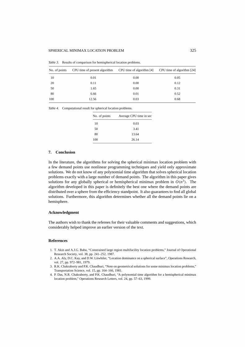
Table 3 compares the algorithm in this paper with the one proposed in [4] and [24]. Thelatter are specifically designed for problems in which all demand points are distributed on ahemisphere. The CPU times in the table are averaged over 50 randomly generated minimaxlocation problems with 10, 20, 50, 80, and 100 demand points.

Similarly, Table 4 reports CPU times on minimax location problems with 10, 50, 80, and100 demand points distributed over a sphere. As before, these times are averaged over a setof 50 randomly generated problems.


Table 3. Results of comparison for hemispherical location problems.

No. of points CPU time of present algorithm CPU time of algorithm [4] CPU time of algorithm [24]

10 0.01 0.00 0.05

20 0.11 0.00 0.12

50 1.65 0.00 0.31

80 6.66 0.01 0.52

100 12.56 0.03 0.68

Table 4. Computational result for spherical location problems.

No. of points Average CPU time in sec

10 0.03

50 3.41

80 13.64

100 26.14

7. Conclusion

In the literature, the algorithms for solving the spherical minimax location problem witha few demand points use nonlinear programming techniques and yield only approximatesolutions. We do not know of any polynomial time algorithm that solves spherical locationproblems exactly with a large number of demand points. The algorithm in this paper givessolutions for any globally spherical or hemispherical minimax problem inO(n3). Thealgorithm developed in this paper is definitely the best one where the demand points aredistributed over a sphere from the efficiency standpoint. It also guarantees to find all globalsolutions. Furthermore, this algorithm determines whether all the demand points lie on ahemisphere.

Acknowledgment

The authors wish to thank the referees for their valuable comments and suggestions, whichconsiderably helped improve an earlier version of the text.

References

1. T. Akin and A.J.G. Babu, “Constrained large region multifacility location problems,” Journal of OperationalResearch Society, vol. 38, pp. 241–252, 1987.

2. A.A. Aly, D.C. Kay, and D.W. Litwhiler, “Location dominance on a spherical surface”, Operations Research,vol. 27, pp. 972–981, 1979.

3. R.K. Chakraborty and P.K. Chaudhuri, “Note on geometrical solutions for some minimax location problems,”Transportation Science, vol. 15, pp. 164–166, 1981.

4. P. Das, N.R. Chakraborty, and P.K. Chaudhuri, “A polynomial time algorithm for a hemispherical minimaxlocation problem,” Operations Research Letters, vol. 24, pp. 57–63, 1999.


5. U.R. Dhar and J.R. Rao, “A comparative study of three norms for facility location problems on sphericalsurface,” New Zealand Journal of Operational Research, vol. 8, pp. 173–183, 1982.

6. U.R. Dhar and J.R. Rao, “Domain approximation method for solving multifacility location problems on asphere,” Journal of Operational Research Society, vol. 33, pp. 639–645, 1982.

7. Z. Drezner, “On location dominance on spherical surfaces,” Operations Research, vol. 29, pp. 1218–1219,1981.

8. Z. Drezner, “Constrained location problems in the plane and on a sphere,” IIE Transactions, vol. 15, pp.300–304, 1983.

9. Z. Drezner and G.O. Wesolowsky, “Facility location on a sphere,” Journal of Operations Research Society,vol. 29, pp. 997–1004, 1978.

10. Z. Drezner and G.O. Wesolowsky, “Minimax and maximin facility location problems on a sphere,” NavalResearch Logistics Quarterly, vol. 30, pp. 305–312, 1983.

11. J. Elzinga and D.W. Hearn, “Geometrical solutions for some minimax location problems,” TransportationScience, vol.6, pp. 379–394, 1972.

12. R.L. Francis, L.F. McGinnis, and J.A. White, Facility Layout and Location: An Analytic Approach, Prenice—Hall: Englewood, N.J., 1992.

13. D.W. Hearn and J. Vijay, “Efficient algorithms for the (Weighted) minimum circle problem,” OperationsResearch, vol. 39, pp. 777–795, 1982.

14. I.N. Katz and L. Cooper, “Optimal location on a sphere,” Computers and Mathematics with Applications, vol.6, pp. 175–196, 1980.

15. D.W. Litwhiler, “Large region location problem,” Ph.D. Thesis, The University of Oklahoma, Norman, O.K,1977.

16. D.W. Litwhiler and A.A. Ally, “Large region location problems,” Computers and Operations Research, vol.6,pp. 1–12, 1979.

17. D.W. Litwhiler and A.A. Ally, “Minimax location problems on the sphere,” I.E. Research Report 81–12(School of Industrial Engineering), University of Oklahoma, Norman, O.K., 1981.

18. R. Love, L.G. Morris, and G.O. Wesolowsky, Facility Location: Models and Methods, North-Holland: NewYork, 1988.

19. N. Megiddo, “Linear time algorithm for linear programming in R3 and related problems,”SIAM J. Comput.,vol. 12, pp. 759–776, 1983.

20. K.P.K. Nair and R. Chandrasekaran, “Optimal location of a single service center of certain types,” NavalResearch Logistics Quarterly, vol. 18, pp. 503–510, 1971.

21. B.J. Oommen, “An efficient geometric solution to minimum spanning circle problem,” Operations Research,vol. 35, pp. 80–86, 1987.

22. M.H. Patel, “Spherical minimax location problem using the Euclidean norm: Formulation and Optimization,”Computational Optimization and Applications, vol. 4, pp. 79–90, 1995.

23. M.H. Patel, D.L. Nettles, and S.J. Deutsch, “A linear programming-based method for determining whether ornotn demand points are on a hemisphere,” Naval Research Logistics, vol. 40, pp. 543–552, 1993.

24. A.K. Sarkar and P.K. Chaudhuri, “Solution of equiweighted minimax problem on a hemisphere,” Computa-tional Optimization and Applications, vol. 6, pp. 73–82, 1996.

25. M.I. Shamos, “Computational geometry,” Ph.D. Thesis, Dept. of Computer Science, Yale University, 1978.26. I. Todhunter and J.G. Leathem, “Spherical trigonometry,” Macmillan & Co. Ltd., 1960.27. W.H. Tsai, M.S. Chern, and T.M. Lin, “An algorithm for determining whetherm demand points are on a

hemisphere or not,” Transportation Science, vol. 25, pp. 91–97, 1991.28. G.O. Wesolowsky, “Location problems on a sphere,” Regional Science Urban Economics, vol. 12, pp. 495–

508, 1982.29. G. Xue and C. Wang, “The Euclidean facilities location problem,” in Advances in Optimization and Approx-

imation, D.Z. Du and J. Sun (Eds.), Kluwer Academic Publishers: Boston, pp. 313–331, 1994.

spherical minimax location problem

Documents