Mach Learn (2011) 85:77–108DOI 10.1007/s10994-011-5252-9

SpicyMKL: a fast algorithm for Multiple KernelLearning with thousands of kernels

Taiji Suzuki · Ryota Tomioka

Received: 28 February 2010 / Accepted: 12 May 2011 / Published online: 3 June 2011© The Author(s) 2011

Abstract We propose a new optimization algorithm for Multiple Kernel Learning (MKL)called SpicyMKL, which is applicable to general convex loss functions and general types ofregularization. The proposed SpicyMKL iteratively solves smooth minimization problems.Thus, there is no need of solving SVM, LP, or QP internally. SpicyMKL can be viewed asa proximal minimization method and converges super-linearly. The cost of inner minimiza-tion is roughly proportional to the number of active kernels. Therefore, when we aim fora sparse kernel combination, our algorithm scales well against increasing number of ker-nels. Moreover, we give a general block-norm formulation of MKL that includes non-sparseregularizations, such as elastic-net and �p-norm regularizations. Extending SpicyMKL, wepropose an efficient optimization method for the general regularization framework. Exper-imental results show that our algorithm is faster than existing methods especially when thenumber of kernels is large (>1000).

Keywords Multiple kernel learning · Sparsity · Non-smooth optimization · Super-linearconvergence · Proximal minimization

1 Introduction

Kernel methods are powerful nonparametric methods in machine learning and data analysis.Typically a kernel method fits a decision function that lies in some Reproducing KernelHilbert Space (RKHS) (Aronszajn 1950; Schölkopf and Smola 2002). In such a learningframework, the choice of a kernel function can strongly influence the performance. Instead

Editors: Süreyya Özögür-Akyüz, Dervim Ünay, Alex Smola.

T. Suzuki (�) · R. TomiokaDepartment of Mathematical Informatics, The University of Tokyo, 7-3-1 Hongo, Bunkyo-ku,Tokyo 113-8656, Japane-mail: t-suzuki@mist.i.u-tokyo.ac.jp

R. Tomiokae-mail: tomioka@mist.i.u-tokyo.ac.jp

78 Mach Learn (2011) 85:77–108

of using a fixed kernel, Multiple Kernel Learning (MKL) (Lanckriet et al. 2004; Bach et al.2004; Micchelli and Pontil 2005) aims to find an optimal combination of multiple candidatekernels.

More specifically, we assume that a data point x ∈ X lies in a space X and we are givenM candidate kernel functions km : X × X → R (m = 1, . . . ,M). Each kernel function corre-sponds to one data source. A conical combination of km (m = 1, . . . ,M) gives the combinedkernel function k = ∑M

m=1 dmkm, where dm is a nonnegative weight. Our goal is to find agood set of kernel weights based on some training examples.

While the MKL framework has opened up a possibility to combine multiple heteroge-neous data sources (numerical features, texts, links) in a principled manner, it is also pos-ing an optimization challenge: the number of kernels can be very large. Instead of arguingwhether polynomial kernel or Gaussian kernel fits a given problem better, we can simplyput both of them into an MKL algorithm; instead of evaluating which band-width parameterto choose, we can simply generate kernels from all the possible combinations of parametervalues and feed them to an MKL algorithm. See Gehler and Nowozin (2009), Tomioka andSuzuki (2009).

Various optimization algorithms have been proposed in the context of MKL. In the pio-neering work of Lanckriet et al. (2004), MKL was formulated as a semi-definite program-ming (SDP) problem. Bach et al. (2004) showed that the SDP can be reduced to a secondorder conic programming (SOCP) problem. However solving SDP or SOCP via generalconvex optimization solver can be quite heavy especially for large number of samples.

More recently, wrapper methods have been proposed. A wrapper method iterativelysolves a single kernel learning problem (e.g., SVM), for a given kernel combination andthen updates the kernel weights. A nice property of this type of methods is that it can makeuse of existing well-tuned solvers for SVM. Semi-Infinite Linear Program (SILP) approachproposed by Sonnenburg et al. (2006) utilizes a cutting plane method for the update of thekernel weights. SILP often suffers from instability of the solution sequence especially whenthe number of kernels is large, i.e. the intermediate solution oscillates around the optimalone (Rakotomamonjy et al. 2008). SimpleMKL proposed by Rakotomamonjy et al. (2008)performs a reduced gradient descent on the kernel weights. Simple MKL resolves the draw-back of SILP, but still it is a first order method. Xu et al. (2009) proposed a novel LevelMethod (which we call LevelMKL) as an improvement of SILP and SimpleMKL. Lev-elMKL is rather efficient than SimpleMKL and scales well against the number of kernelsby utilizing sparsity but it shows unstable behavior as the algorithm proceeds because Lev-elMKL solves Linear Programming (LP) and Quadratic Programming (QP) of increasinglylarge size as its iteration proceeds. HessianMKL proposed by Chapelle and Rakotomamonjy(2008) replaced the gradient descent update of SimpleMKL with a Newton update. At eachiteration, HessianMKL solves a QP problem with the size of the number of kernels to ob-tain the Newton update direction. HessianMKL shows second order convergence, but scalesbadly against the number of kernels because the size of the QP grows as the number ofkernels grows.

The first contribution of this article is an efficient optimization algorithm for MKL basedon the block 1-norm formulation introduced in Bach et al. (2005) (see also Bach et al.2004); see (4). The block 1-norm formulation can be viewed as a kernelized version ofgroup lasso (Yuan and Lin 2006; Bach 2008). For group lasso, or more generally sparseestimation, efficient optimization algorithms have recently been studied intensively, boostedby the development of compressive sensing theory (Candes et al. 2006). Based on this view,we extend the dual augmented-Lagrangian (DAL) algorithm (Tomioka and Sugiyama 2009)recently proposed in the context of sparse estimation to kernel-based learning. DAL is ef-ficient when the number of unknown variables is much larger than the number of samples.

Mach Learn (2011) 85:77–108 79

This enables us to scale the proposed algorithm, which we call SpicyMKL, to thousands ofkernels.

Compared to the original DAL algorithm (Tomioka and Sugiyama 2009), our presenta-tion is based on an application of proximal minimization framework (Rockafellar 1976) tothe primal MKL problem. We believe that the current formulation is more transparent com-pared to the dual based formulation in Tomioka and Sugiyama (2009), because we are notnecessarily interested in solving the dual problem. Moreover, we present a theorem on therate of convergence.

SpicyMKL does not need to solve SVM, LP or QP internally as previous approaches.Instead, it minimizes a smooth function at every step. The cost of inner minimization isproportional to the number of active kernels. Therefore, when we aim for a sparse kernelcombination, the proposed algorithm is efficient even when thousands of candidate kernelsare used. In fact, we show numerically that we are able to train a classifier with 3000 kernelsin less than 10 seconds.

Learning combination of kernels, however, has recently recognized as a more complextask than initially thought. Cortes (2009) pointed out that learning convex kernel combi-nation with an �1-constraint on the kernel weights (see Sect. 2) produces an overly sparse(many kernel weights are zero) solution, and it is often outperformed by a simple uniformcombination of kernels; accordingly they proposed to use an �2-constraint instead (Corteset al. 2009). In order to search for the best trade-off between the sparse �1-MKL and theuniform weight combination, Kloft et al. (2009) proposed a general �p-norm constraint andTomioka and Suzuki (2009) proposed an elastic-net regularization, both of which smoothlyconnect the 1-norm MKL and uniform weight combination.

The second contribution of this paper is to extend the block-norm formulation that al-lows us to view these generalized MKL models in a unified way, and provide an efficientoptimization algorithm. We note that while this paper was under review, Kloft et al. (2010)presented a slightly different approach that results in a similar optimization algorithm. How-ever, our formulation provides clearer relationship between the block-norm formulation andkernel-combination weights and is more general.

This article is organized as follows. In Sect. 2, we introduce the framework of block 1-norm MKL through Tikhonov regularization on the kernel weights. In Sect. 3, we propose anextension of DAL algorithm to kernel-learning setting. Our formulation of DAL algorithm isbased on a primal application of the proximal minimization framework (Rockafellar 1976),which also sheds a new light on DAL algorithm itself. Furthermore, we discuss how wecan carry out the inner minimization efficiently exploiting the sparsity of the 1-norm MKL.In Sect. 4, we extend our framework to general class of regularizers including the �p-normMKL (Kloft et al. 2009) and Elastic-net MKL (Tomioka and Suzuki 2009). We extend theproposed SpicyMKL algorithm for the generalized formulation and also present a simpleone-step optimization procedure for some special cases that include Elastic-net MKL and�p-norm MKL. In Sect. 5, we discuss the relations between the existing methods and theproposed method. In Sect. 6, we show the results of numerical experiments. The experi-ments show that SpicyMKL is efficient for block 1-norm regularization especially when thenumber of kernels is large. Moreover the one-step optimization procedure for elastic-netregularization shows quite fast convergence. In fact, it is faster than those methods withblock 1-norm regularization. Finally, we summarize our contribution in Sect. 7. The proofof super-linear convergence of the proposed SpicyMKL is given in Appendix.

A Matlab R© implementation of SpicyMKL is available at the following URL: http://www.simplex.t.u-tokyo.ac.jp/~s-taiji/software/SpicyMKL.

80 Mach Learn (2011) 85:77–108

2 Framework of MKL

In this section, we first consider a learning problem with fixed kernel weights in Sect. 2.1.Next in Sect. 2.2, using Tikhonov regularization on the kernel weights, we derive a block1-norm formulation of MKL, which can be considered as a direct extension of group lassoin the kernel-based learning setting. In addition, we discuss the connection between thecurrent block 1-norm formulation and the squared block 1-norm formulation. In Sect. 2.3,we present a finite dimensional version of the proposed formulation and prepare notationsfor the later sections.

2.1 Fixed kernel combination

We assume that we are given N samples (xi, yi)Ni=1 where xi belongs to an input space X

and yi belongs to an output space Y (usual settings are Y = {±1} for classification andY = R for regression). We define the Gram matrix with respect to the kernel function km asKm = (km(xi, xj ))i,j . We assume that the Gram matrix Km is positive definite.1

We first consider a learning problem with fixed kernel weights. More specifically, we fixnon-negative kernel weights d1, d2, . . . , dM and consider the RKHS H corresponding to thecombined kernel function k = ∑M

m=1 dmkm. The (squared) RKHS norm of a function f in His written as follows (see Sect. 6 in Aronszajn 1950, and also Micchelli and Pontil 2005):

‖f ‖2H := min

f1∈H1,...,fM∈HM

M∑

m=1

‖fm‖2Hm

dm

s.t. f =M∑

m=1

fm, (1)

where Hm is the RKHS that corresponds to the kernel function km. Accordingly, with a fixedkernel combination, a supervised learning problem can be written as follows:

minimizef1∈H1,...,fM∈HM,b∈R

N∑

i=1

�

(

yi,

M∑

m=1

fm(xi) + b

)

+ C

2

M∑

m=1

‖fm‖2Hm

dm

, (2)

where b is a bias term and �(y,f ) is a loss function, which can be the hinge loss max(1 −yf,0) or the logistic loss log(1 + exp(−yf )) for a classification problem, or the squaredloss (y − f )2 or the SVR loss max(|y − f | − ε,0) for a regression problem. The aboveformulation may not be so useful in practice, because we can compute the combined kernelfunction k and optimize over f instead of optimizing M functions f1, . . . , fM . However,explicitly handling the kernel weights allows us to consider various generalizations of MKLin a unified manner.

2.2 Learning kernel weights

In order to learn the kernel weights dm through the objective (2), there is clearly a needfor regularization, because the objective is a decreasing function of the kernel weights dm.Roughly speaking, the kernel weight dm corresponds to the complexity allowed for the mthclassifier component fm, without regularization, we can get a serious over-fitting.

1To avoid numerical instability, we added 10−8 to diagonal elements of Km in the numerical experiments.

Mach Learn (2011) 85:77–108 81

One way to prevent such overfitting is to penalize the increase of the kernel weight dm

by adding a penalty term. Adding a linear penalty term, we have the following optimizationproblem:

minimizef1∈H1,...,fM∈HM,

b∈R,d1≥0,...,dM≥0

N∑

i=1

�

(

yi,

M∑

m=1

fm(xi) + b

)

+ C

2

M∑

m=1

(‖fm‖2Hm

dm

+ dm

)

. (3)

The above formulation reduces to the block 1-norm introduced in Bach et al. (2005) byexplicitly minimizing over dm as follows:

minimizef1∈H1,...,fM∈HM,

b∈R

N∑

i=1

�

(

yi,

M∑

m=1

fm(xi) + b

)

+ C

M∑

m=1

‖fm‖Hm, (4)

where we used the inequality of arithmetic and geometric means; the minimum with respectto dm is obtained by taking dm = ‖fm‖Hm .

The regularization term in the above block 1-norm formulation is the linear sum of RKHSnorms. This formulation can be seen as a direct generalization of group lasso (Yuan and Lin2006) to the kernel-based learning setting, and motivates us to extend an efficient algorithmfor sparse estimation to MKL.

The block 1-norm formulation (4) is related to the following squared block 1-norm for-mulation considered in Bach et al. (2004), Sonnenburg et al. (2006), Zien and Ong (2007),Rakotomamonjy et al. (2008):

minimizef1∈H1,...,fM∈HM,b∈R

N∑

i=1

�

(

yi,

M∑

m=1

fm(xi) + b

)

+ C

2

(M∑

m=1

‖fm‖Hm

)2

, (5)

which is obtained by considering a simplex constraint on the kernel weights (Kloft et al.2009) instead of penalizing them as in (3).

The solution of the two problems (4) and (5) can be mapped to each other. In fact, let{f �

m}Mm=1 be the minimizer of the block 1-norm formulation (4) with the regularization pa-

rameter C and let C be

C = C

(M∑

m=1

‖f �m‖Hm

)

. (6)

Then {f �m} also minimizes the squared block 1-norm formulation (5) with the regularization

parameter C because of the relation

∂fm

1

2

(M∑

m=1

‖fm‖Hm

)2

=(

M∑

m=1

‖fm‖Hm

)

∂fm‖fm‖Hm,

where ∂fm is a subdifferential with respect to fm.

2.3 Representer theorem

In this subsection, we convert the block 1-norm MKL formulation (4) into a finite dimen-sional optimization problem via the representer theorem and prepare notation for later sec-tions.

82 Mach Learn (2011) 85:77–108

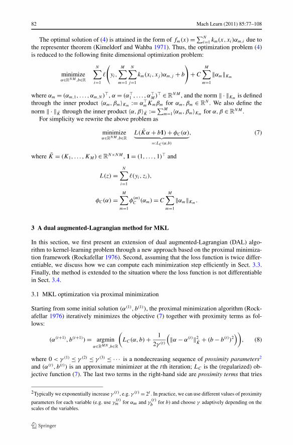
The optimal solution of (4) is attained in the form of fm(x) = ∑N

i=1 km(x, xi)αm,i due tothe representer theorem (Kimeldorf and Wahba 1971). Thus, the optimization problem (4)is reduced to the following finite dimensional optimization problem:

minimizeα∈RNM,b∈R

N∑

i=1

�

(

yi,

M∑

m=1

N∑

j=1

km(xi, xj )αm,j + b

)

+ C

M∑

m=1

‖αm‖Km

where αm = (αm,1, . . . , αm,N )�, α = (α�1 , . . . , α�

M)� ∈ RNM , and the norm ‖ · ‖Km is defined

through the inner product 〈αm,βm〉Km := α�mKmβm for αm,βm ∈ R

N . We also define thenorm ‖ · ‖K through the inner product 〈α,β〉K := ∑M

m=1〈αm,βm〉Km for α,β ∈ RNM .

For simplicity we rewrite the above problem as

minimizeα∈RNM,b∈R

L(Kα + b1) + φC(α)︸ ︷︷ ︸

=:LC(α,b)

, (7)

where K = (K1, . . . ,KM) ∈ RN×NM , 1 = (1, . . . ,1)� and

L(z) =N∑

i=1

�(yi, zi),

φC(α) =M∑

m=1

φ(m)C (αm) = C

M∑

m=1

‖αm‖Km.

3 A dual augmented-Lagrangian method for MKL

In this section, we first present an extension of dual augmented-Lagrangian (DAL) algo-rithm to kernel-learning problem through a new approach based on the proximal minimiza-tion framework (Rockafellar 1976). Second, assuming that the loss function is twice differ-entiable, we discuss how we can compute each minimization step efficiently in Sect. 3.3.Finally, the method is extended to the situation where the loss function is not differentiablein Sect. 3.4.

3.1 MKL optimization via proximal minimization

Starting from some initial solution (α(1), b(1)), the proximal minimization algorithm (Rock-afellar 1976) iteratively minimizes the objective (7) together with proximity terms as fol-lows:

(α(t+1), b(t+1)) = argminα∈RMN ,b∈R

(

LC(α,b) + 1

2γ (t)

(‖α − α(t)‖2

K+ (b − b(t))2

))

, (8)

where 0 < γ (1) ≤ γ (2) ≤ γ (3) ≤ · · · is a nondecreasing sequence of proximity parameters2

and (α(t), b(t)) is an approximate minimizer at the t th iteration; LC is the (regularized) ob-jective function (7). The last two terms in the right-hand side are proximity terms that tries

2Typically we exponentially increase γ (t), e.g. γ (t) = 2t . In practice, we can use different values of proximity

parameters for each variable (e.g. use γ(t)m for αm and γ

(t)b

for b) and choose γ adaptively depending on thescales of the variables.

Mach Learn (2011) 85:77–108 83

to keep the next solution (α(t+1), b(t+1)) close to the current solution (α(t), b(t)). Thus, wecall the minimization problem (8) a proximal MKL problem. Solving the proximal MKLproblem (8) seems as difficult as solving the original MKL problem in the primal. However,when we consider the dual problems, solving the dual of proximal MKL problem (8) is asmooth minimization problem and can be minimized efficiently, whereas solving the dual ofthe original MKL problem (7) is a non-smooth minimization problem and not necessarilyeasier than solving the primal.

The update equation can be interpreted as an implicit gradient method on the objectivefunction LC(α,b). In fact, by taking the subgradient of the update equation (8) and equatingit to zero, we have

α(t+1)m ∈ α(t)

m − γ (t)K−1m ∂αmLC(α(t+1), b(t+1)),

b(t+1) ∈ b(t) − γ (t)∂bLC(α(t+1), b(t+1)).

This implies the t th update step is a subgradient of the original objective function LC at thenext solution (α(t+1)

m , b(t+1)).The super-linear convergence of proximal minimization algorithm (Rockafellar 1976;

Bertsekas 1982; Tomioka et al. 2011) can also be extended to kernel-based learning settingas in the following theorem.

Theorem 1 Suppose the problem (7) has a unique3 optimal solution α∗, b∗, and there exista scalar σ > 0 and a δ-neighborhood (δ > 0) of the optimal solution such that

LC(α,b) ≥ LC(α∗, b∗) + σ(‖α − α∗‖2K

+ (b − b∗)2), (9)

for all (α, b) ∈ RMN × R satisfying ‖α − α∗‖2

K+ (b − b∗)2 ≤ δ2. Then for all sufficiently

large t we have

‖α(t+1) − α∗‖2K

+ (b(t+1) − b∗)2

‖α(t) − α∗‖2K

+ (b(t) − b∗)2≤ 1

(1 + σγ (t))2.

Therefore if limt→∞ γ (t) = ∞, the solution (α(t), b(t)) converges to the optimal solutionsuper-linearly.

Proof The proof is given in Appendix. �

3.2 Derivation of SpicyMKL

Although directly minimizing the proximal MKL problem (8) is not a trivial task, its dualproblem can efficiently be solved. Once we solve the dual of the proximal minimizationupdate (8), we can update the primal variables (α(t), b(t)). The resulting iteration can bewritten as follows:

ρ(t) := argminρ∈RN

ϕγ (t) (ρ;α(t), b(t)), (10)

α(t+1)m = prox(α(t)

m + γ (t)ρ(t)|φ(m)

γ (t)C) (m = 1, . . . ,M), (11)

3The uniqueness of the optimal solution is just for simplicity. The result can be generalized for a compactoptimal solution set (see Bertsekas 1982).

84 Mach Learn (2011) 85:77–108

b(t+1) = b(t) + γ (t)

N∑

i=1

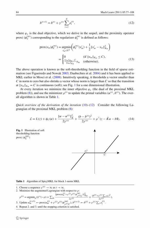
ρ(t)i , (12)

where ϕγ is the dual objective, which we derive in the sequel, and the proximity operatorprox(·|φ(m)

C ) corresponding to the regularizer φ(m)C is defined as follows:

prox(vm|φ(m)C ) = argmin

v′m∈RN

(

φ(m)C (v′

m) + 1

2‖v′

m − vm‖2Km

)

={

0 (if ‖vm‖Km ≤ C),‖vm‖Km−C

‖vm‖Kmvm (otherwise).

(13)

The above operation is known as the soft-thresholding function in the field of sparse esti-mation (see Figueiredo and Nowak 2003; Daubechies et al. 2004) and it has been applied toMKL earlier in Mosci et al. (2008). Intuitively speaking, it thresholds a vector smaller thanC in norm to zero but also shrinks a vector whose norm is larger than C so that the transitionat ‖vm‖Km = C is continuous (soft); see Fig. 1 for a one dimensional illustration.

At every iteration we minimize the inner objective ϕγ (the dual of the proximal MKLproblem (8)), and use the minimizer ρ(t) to update the primal variables (α(t), b(t)). The over-all algorithm is shown in Table 1.

Quick overview of the derivation of the iteration (10)–(12) Consider the following La-grangian of the proximal MKL problem (8):

L = L(z) + φC(α) + ‖α − α(t)‖2K

2γ (t)+ (b − b(t))2

2γ (t)+ ρ�(z − Kα − b1), (14)

Fig. 1 Illustration of softthresholding function

prox(·|φ(m)C

)

Table 1 Algorithm of SpicyMKL for block 1-norm MKL

1. Choose a sequence γ (t) → ∞ as t → ∞.2. Minimize the augmented Lagrangian with respect to ρ:

ρ(t) = argminρ(L∗(−ρ) + ∑m

‖prox(α(t)m +γ (t)ρ(t)|φ(m)

γ (t)C)‖2

Km

2γ (t) + (b(t)+γ (t) ∑i ρi )

2

2γ (t) ).

3. Update α(t+1)m ← prox(α

(t)m + γ (t)ρ(t)|φ(m)

γ (t)C), b(t+1) ← b(t) + γ (t)

∑i ρ

(t)i

.

4. Repeat 2. and 3. until the stopping criterion is satisfied.

Mach Learn (2011) 85:77–108 85

where ρ ∈ RN is the Lagrangian multiplier corresponding to the equality constraint z =

Kα + b1. The vector ρ(t) in the first step (10) is the optimal Lagrangian multiplier thatmaximizes the dual of the proximal MKL problem (8) (see (25)). The remaining steps (11)–(12) can be obtained by minimizing the above Lagrangian with respect to α and b for ρ =ρ(t), respectively.

Detailed derivation of the iteration (10)–(12) Let’s consider the constraint reformulationof the proximal MKL problem (8) as follows:

minimizeα∈R

MN ,b∈R

z∈RN

L(z) + φC(α) + ‖α − α(t)‖2K

2γ (t)+ (b − b(t))2

2γ (t),

subject to z = Kα + b1.

The Lagrangian of the above constrained minimization problem can be written as in (14).The dual problem can be derived by minimizing the Lagrangian (14) with respect to the

primal variables (z,α, b). See (25) for the final expression. Note that the minimization isseparable into minimization with respect to z (15), α (20), and b (24).

First, minimizing the Lagrangian with respect to z gives

minz∈RN

(L(z) + ρ�z

) = −L∗(−ρ), (15)

where L∗ is the convex conjugate of the loss function L as follows:

L∗(−ρ) := supz∈RN

((−ρ)�z − L(z)

)

=N∑

i=1

(−ρizi − �(yi, zi))

=N∑

i=1

�∗(yi,−ρi),

where �∗ is the convex conjugate of the loss � with respect to the second argument.For example, the conjugate loss �∗

L for the logistic loss �L is the negative entropy functionas follows:

�∗L(y,−ρ) =

{(yρ) log(yρ) + (1 − yρ) log(1 − yρ) (if 0 ≤ yρ ≤ 1),

+∞ (otherwise).(16)

The conjugate loss �∗H for the hinge loss �H is given as follows:

�∗H (y,−ρ) =

{−yρ (if 0 ≤ yρ ≤ 1),

+∞ (otherwise).(17)

Second, minimizing the Lagrangian (14) with respect to α, we obtain

minα∈RMN

(

φC(α) + ‖α − α(t)‖2K

2γ (t)− ρ�Kα

)

86 Mach Learn (2011) 85:77–108

= minα∈RMN

(

φC(α) + ‖α − α(t) − γ (t)ρ‖2K

2γ (t)

)

− ‖α(t) + γ (t)ρ‖2K

2γ (t)+ const (18)

(21),(23)= − 1

γ (t)min

u∈RMN

(

δγ (t)C(u) + ‖u − α(t) − γ (t)ρ‖2K

2

)

+ const (19)

(22)= − 1

γ (t)

M∑

m=1

�(m)

γ (t)C(αm + γ (t)ρ) + const, (20)

where const is a term that only depends on α(t) and γ (t); the function δC : RMN → R is the

convex conjugate of the regularization term φ(m)C (αm) = C‖αm‖Km as follows:

δC(u) :=M∑

m=1

δ(m)C (um),

where

δ(m)C (um) := sup

αm∈RN

(〈um,αm〉Km

− φ(m)C (αm)

)

= supαm∈RN

(‖um‖Km‖αm‖Km − C‖αm‖Km

)

={

0 (if ‖um‖Km ≤ C),

+∞ (otherwise).(21)

See Fig. 2 for a one dimensional illustration of the conjugate regularizer δ(m)C . In addition,

the function �(m)C in the last line is Moreau’s envelope function (see Fig. 2):

�(m)C (vm) := min

v′m∈RN

(

δ(m)C (v′

m) + 1

2‖v′

m − vm‖2Km

)

,

=∥∥∥prox(vm|φ(m)

C )

∥∥∥

2

Km

. (22)

See (13) and Fig. 1 for the definition of the soft-threshold operation prox(·|φ(m)C ). Further-

more, we used the following proposition and some algebra to derive (19) from (18).

Proposition 1 Let f : Rn → R be a closed proper convex function and f ∗ be the convex

conjugate of f defined as

f ∗(y) = supx∈Rn

(〈y, x〉K − f (x)) ,

where K ∈ Rn×n is a positive semidefinite matrix. Then

minx∈Rn

(

f (x) + ‖x − z‖2K

2

)

+ miny∈Rn

(

f ∗(y) + ‖y − z‖2K

2

)

= ‖z‖2K

2. (23)

Mach Learn (2011) 85:77–108 87

Fig. 2 Comparison of the

conjugate regularizer δ(m)C

andthe corresponding Moreau’s

envelope function �(m)C

in onedimension. The conjugate

regularizer δ(m)C

(21) isnondifferentiable at the boundaryof its domain, whereas itsenvelope function �

(m)C

issmooth

Proof It is a straightforward generalization of Moreau’s theorem. See Rockafellar (1970,Theorem 31.5) and Tomioka et al. (2011). �

Finally, minimizing the Lagrangian (14) with respect to b, we obtain

minb∈R

((b − b(t))2

2γ (t)− bρ�1

)

= − (b(t) + γ (t)ρ�1)2

2γ (t)+ const, (24)

where const is a term that only depends on b(t) and γ (t).Combining (15), (20), and (24), the dual of the proximal MKL problem (8) can be ob-

tained as follows:

maximizeρ∈RN

− L∗(−ρ) − 1

2γ (t)

M∑

m=1

∥∥∥prox(α(t)

m + γ (t)ρ|φ(m)

γ (t)C)

∥∥∥

2

Km

− 1

2γ (t)

(

b(t) + γ (t)

N∑

i=1

ρi

)2

, (25)

where the constant terms are ignored. We denote the maximand in the above dual problemby −ϕγ (t) (ρ;α(t), b(t)); see (10).

3.3 Minimizing the inner objective function

The inner objective function (25) that we need to minimize at every iteration is convex anddifferentiable when L∗ is differentiable. In fact, the gradient and the Hessian of the innerobjective ϕγ can be written as follows:

∇ρϕγ (ρ;α,b) = −∇ρL∗(−ρ) +

(

b + γ∑

i

ρi

)

1 +∑

m∈M+Kmprox

(αm + γρ

∣∣φ(m)

γC

), (26)

∇2ρϕγ (ρ;α,b) = ∇2

ρL∗(−ρ) + γ 11� + γ

∑

m∈M+

((1 − qm)Km + qmKmvmv�

mKm

), (27)

where M+ is the set of indices corresponding to the active kernels; i.e., M+ = {m ∈{1, . . . ,M} | ‖αm + γ ρ‖Km > γ C}; for m ∈ M+, a scalar qm and a vector vm ∈ R

N aredefined as qm := γ C

‖αm+γ ρ‖Kmand vm := (αm + γ ρ)/‖αm + γ ρ‖Km .

88 Mach Learn (2011) 85:77–108

Remark 1 The computation of the objective ϕγ (ρ;α,b) (25), the gradient (26), and theHessian (27) is efficient because they require only the terms corresponding to the activekernels {km | m ∈ M+}.

The above sparsity, which makes the proposed algorithm efficient, comes from our dualformulation. By taking the dual, there appears flat region (see Fig. 2); i.e. the region {ρ |prox(α(t)

m + γ (t)ρ|φ(m)

γ (t)C) = 0} is not a single point but has its interior.

Since the inner objective function (25) is differentiable, and the sparsity of the interme-diate solution can be exploited to evaluate the gradient and Hessian of the inner objective,the inner minimization can efficiently be carried out. We call the proposed algorithm SparseIterative MKL (SpicyMKL). The update equations (11)–(12) exactly correspond to the aug-mented Lagrangian method for the dual of the problem (7) (see Tomioka and Sugiyama2009) but derived in more general way using the techniques from Rockafellar (1976).

We use the Newton method with line search for the minimization of the inner objec-tive (25). The line search is used to keep ρ inside the domain of the dual loss L∗. This workswhen the gradient of the dual loss L∗ is unbounded at the boundary of its domain, for ex-ample the logistic loss (16), in which case the minimum is never attained at the boundary.On the other hand, for the hinge loss (17), the solution lies typically at the boundary of thedomain 0 ≤ yρ ≤ 1. This situation is handled separately in the next subsection.

3.4 Explicitly handling boundary constraints

The Newton method with line search described in the last section is unsuitable when theconjugate loss function �∗(y, ·) has a non-differentiable point in the interior of its domain orit has finite gradient at the boundary of its domain. We use the same augmented Lagrangiantechnique for these cases. More specifically we introduce additional primal variables so thatthe AL function ϕγ (·;α,b) becomes differentiable. First we explain this in the case of hingeloss for classification. Next we discuss a generalization to other cases.

3.4.1 Optimization for hinge loss

Here we explain how the augmented Lagrangian technique is applied to the hingeloss. To this end, we introduce two sets of slack variables ξ = (ξ1, . . . , ξN)� ≥ 0, ζ =(ζ1, . . . , ζN)� ≥ 0 as in standard SVM literature (see e.g., Schölkopf and Smola 2002). Thebasic update equation (8) is rewritten as follows:4

(α(t+1), b(t+1), ξ (t+1), ζ (t+1))

= argminα∈R

(MN),b∈R

ξ∈RN+ ,ζ∈R

N+

{

HC(α,b, ξ, ζ ) + 1

2γ (t)

(‖α − α(t)‖2

K+ (b − b(t))2

+ ‖ξ − ξ (t)‖2 + ‖ζ − ζ (t)‖2)}

,

4R+ is the set of non-negative real numbers.

Mach Learn (2011) 85:77–108 89

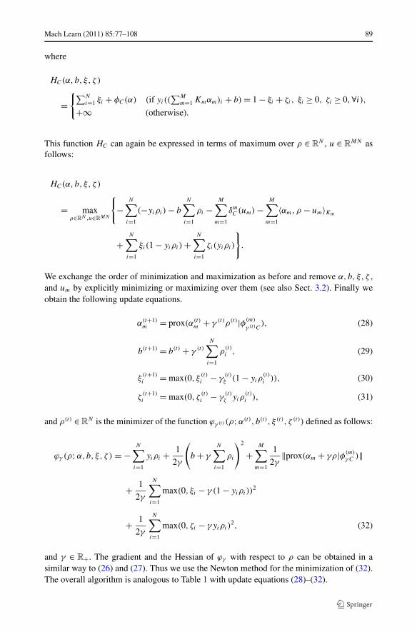
where

HC(α,b, ξ, ζ )

={∑N

i=1 ξi + φC(α) (if yi((∑M

m=1 Kmαm)i + b) = 1 − ξi + ζi, ξi ≥ 0, ζi ≥ 0,∀i),

+∞ (otherwise).

This function HC can again be expressed in terms of maximum over ρ ∈ RN , u ∈ R

MN asfollows:

HC(α,b, ξ, ζ )

= maxρ∈RN ,u∈RMN

{

−N∑

i=1

(−yiρi) − b

N∑

i=1

ρi −M∑

m=1

δmC (um) −

M∑

m=1

〈αm,ρ − um〉Km

+N∑

i=1

ξi(1 − yiρi) +N∑

i=1

ζi(yiρi)

}

.

We exchange the order of minimization and maximization as before and remove α,b, ξ, ζ ,and um by explicitly minimizing or maximizing over them (see also Sect. 3.2). Finally weobtain the following update equations.

α(t+1)m = prox(α(t)

m + γ (t)ρ(t)|φ(m)

γ (t)C), (28)

b(t+1) = b(t) + γ (t)

N∑

i=1

ρ(t)i , (29)

ξ(t+1)i = max(0, ξ

(t)i − γ

(t)ξ (1 − yiρ

(t)i )), (30)

ζ(t+1)i = max(0, ζ

(t)i − γ

(t)ζ yiρ

(t)i ), (31)

and ρ(t) ∈ RN is the minimizer of the function ϕγ (t) (ρ;α(t), b(t), ξ (t), ζ (t)) defined as follows:

ϕγ (ρ;α,b, ξ, ζ ) = −N∑

i=1

yiρi + 1

2γ

(

b + γ

N∑

i=1

ρi

)2

+M∑

m=1

1

2γ‖prox(αm + γρ|φ(m)

γC )‖

+ 1

2γ

N∑

i=1

max(0, ξi − γ (1 − yiρi))2

+ 1

2γ

N∑

i=1

max(0, ζi − γyiρi)2, (32)

and γ ∈ R+. The gradient and the Hessian of ϕγ with respect to ρ can be obtained in asimilar way to (26) and (27). Thus we use the Newton method for the minimization of (32).The overall algorithm is analogous to Table 1 with update equations (28)–(32).

90 Mach Learn (2011) 85:77–108

3.4.2 Optimization for general loss functions with constraints

Here we generalize the above argument to a broader class of loss functions. We assume thatthe dual of the loss function can be written by using twice differentiable convex functions�0 and hj as

�∗(yi, ρi) = minρi

{�∗0(yi, (ρi, ρi)) | hj (yi, (ρi, ρi)) ≤ 0 (1 ≤ j ≤ B)}, (33)

where ρi ∈ RB ′

is an auxiliary variable and we set the right hand side as ∞ if there is nofeasible ρi satisfying hj (yi, (ρi, ρi)) ≤ 0 (1 ≤ j ≤ B). An example is ε-sensitive loss forregression that is defined as

�(y,f ) ={

|f − y| − ε (if |f − y| ≥ ε),

0 (otherwise).

By simple calculation, the dual function of the ε-sensitive loss is given as

�∗(y,ρ) ={

yρ + |ρ|ε (if |ρ| ≤ 1),

∞ (otherwise).(34)

This is not differentiable, but is written as

�∗(y,ρ) ={

minρ∈R{yρ + (ρ + 2ρ)ε | −ρ ≤ 0,−ρ − ρ ≤ 0} (if − 1 ≤ ρ ≤ 1),

∞ (otherwise).(35)

Thus in this example, �∗0(y, (ρ, ρ)) = yρ + (ρ + 2ρ), h1(y, (ρ, ρ)) = ρ − 1, h2(y, (ρ, ρ)) =

−1 − ρ, h3(y, (ρ, ρ)) = −ρ, and h4(y, (ρ, ρ)) = −ρ − ρ in the formulation of (33).The update equation becomes as following:

(α(t+1), b(t+1), ξ (t+1)) (36)

= argminα∈R

(MN),b∈R

ξ∈RNB+

{

HC(α,b, ξ) + 1

2γ (t)

(‖α − α(t)‖2K

+ (b − b(t))2 + ‖ξ − ξ (t)‖2)}

, (37)

where HC is expressed in terms of maximum over ρ ∈ RN , ρ ∈ R

NB ′, u ∈ R

MN as follows:

HC(α,b, ξ)

= maxρ∈RN ,ρ∈RNB′

,u∈RMN

{

−N∑

i=1

�∗0(yi, (−ρi, ρi)) −

M∑

m=1

δmC (um) −

M∑

m=1

〈αm,ρ − um〉Km

− b

N∑

i=1

ρi −N∑

i=1

B∑

j=1

ξi,j hj (yi, (−ρi, ρi))

}

.

Note that the minimum of HC(α,b, ξ) with respect to ξ is the primal objective functionL(Kα + b1) + φC(α) because by exchanging min and max we have

Mach Learn (2011) 85:77–108 91

minξ∈R

NB+HC(α,b, ξ)

= maxρ∈R

N

ρ∈RNB′

,u∈RMN

infξ∈R

NB+

{

−N∑

i=1

�∗0(yi, (−ρi, ρi)) −

M∑

m=1

δmC (um) −

M∑

m=1

〈αm,ρ − um〉Km

− b

N∑

i=1

ρi −N∑

i=1

B∑

j=1

ξi,j hj (yi, (−ρi, ρi))

}

= maxρ∈RN ρ∈RNB′

{

−N∑

i=1

�∗0(yi, (−ρi, ρi)) + ρ�(Kα + b1) | hj (yi, (−ρi, ρi)) ≤ 0 (∀i, j)

}

+ maxu∈RMN

{

−M∑

m=1

δmC (um) +

M∑

m=1

〈αm,um〉Km

}

= L(Kα + b1) + φC(α).

However it is difficult to directly optimize the primal objective. Therefore we add the penaltyterm as in (37) and solve its dual problem. We exchange the order of minimization and max-imization as in the last section (see also Sect. 3.2) and remove α,b, ξ , and um by explicitlyminimizing or maximizing over them. Finally we obtain the following update equations.

α(t+1)m = prox(α(t)

m + γ (t)ρ(t)|φ(m)

γ (t)C), (38)

b(t+1) = b(t) + γ (t)

N∑

i=1

ρ(t)i , (39)

ξ(t+1)i,j = max(0, ξ

(t)i,j − γ (t)hj (yi, (−ρ

(t)i , ρ

(t)i ))), (40)

where (ρ(t), ρ(t)) ∈ RN × R

NB ′is the minimizer of the function ϕγ (t) (ρ, ρ;α(t), b(t), ξ (t))

defined as follows:

ϕγ (ρ, ρ;α,b, ξ)

=N∑

i=1

�∗0(yi, (−ρi, ρi)) + 1

2γ

(

b + γ

N∑

i=1

ρi

)2

+M∑

m=1

1

2γ‖prox(αm + γρ|φ(m)

γC )‖2Km

+ 1

2γ

N∑

i=1

B∑

j=1

max(0, ξi,j − γ hj (yi, (−ρi, ρi)))2, (41)

and γ ∈ R+. The gradient and the Hessian of ϕγ with respect to (ρ, ρ) can be obtained in asimilar way to (26) and (27). Thus we use the Newton method for the minimization of ϕγ (t)

(32). The overall algorithm is summarized in Table 2.

92 Mach Learn (2011) 85:77–108

Table 2 Algorithm of SpicyMKL for a general regularization term and a general loss function

1. Choose a sequence γ (t) → ∞ as t → ∞.2. Minimize the augmented Lagrangian with respect to ρ and ρ:

(ρ(t), ρ(t)) = argminρ,ρ (∑

i �∗0(yi , (−ρi , ρi )) + 1

2γ (t)

∑m ‖prox(α

(t)m + γ (t)ρ|φ(m)

γ (t)C)‖2

Km

+ 12γ (t)

∑Ni=1

∑Bj=1 max(0, ξ

(t)i,j

− γ hj (yi , (−ρi , ρi )))2 + 1

2γ (t) (b(t) + γ (t)∑

i ρi )2).

3. Update α(t+1)m ← prox(α

(t)m + γ (t)ρ(t)|φm

γ (t)C), b(t+1) ← b(t) + γ (t)

∑i ρ

(t)i

,

ξ(t+1)i,j

← max(0, ξ(t)i,j

− γ (t)hj (yi , (ρ(t)i

, ρ(t)i

))).

4. Repeat 2. and 3. until the stopping criterion is satisfied.

3.5 Technical details of computations

3.5.1 Back-tracking in the Newton update

We use back-tracking line search with Armijo’s rule to find a step size of the Newton method.During the back-tracking, the computational bottle-neck is the computation of the norm‖ρ +c�ρ + αm

γm‖Km (m = 1, . . . ,M) where �ρ is the Newton update direction and 0 < c ≤ 1

is a step size. However, the above computation is necessary only for the active kernels M+;for example, the active kernels M+ is included in {m | ‖ρ + αm

γm‖Km > C or ‖ρ + �ρ +

αm

γm‖Km > C} for block 1-norm MKL and {m | ‖ρ‖Km > (1 − λ)C or ‖ρ + �ρ‖Km > (1 −

λ)C} for Elastic-net MKL because of the convexity of ‖ · ‖Km . This reduces the computationtime considerably.

3.5.2 Parallelization in the computation of ‖α(t)m + ρ(t)

γ(t)m

‖Km

The computation of ‖α(t)m + ρ(t)

γ(t)m

‖Km for m = 1, . . . ,M is necessary at every outer iteration.

Thus when the number of kernels is large, its cost cannot be ignored. Fortunately, the compu-tation with respect to the m-th kernel is independent of the others and the outer loop is easilyparallelizable. In our experiments, we implemented the parallel computing by OpenMP inmex-files of our Matlab� code. We observed twenty or thirty percent improvement of over-all computational time by the parallelization.

4 Generalized block-norm formulation

Motivated by the recent interest in non-sparse regularization for MKL, we consider a gen-eralized block norm formulation in this section. The proposed formulation uses a concavefunction g and it subsumes previously proposed MKL models, such as �p-norm MKL (Kloftet al. 2009) and Elastic-net MKL (Tomioka and Suzuki 2009), as different choices of theconcave function g. Moreover, using a convex upper-bounding technique (Palmer et al.2006) we show that the proposed formulation can be written also as a Tikhonov regular-ization problem (3). Thus the solution can be easily mapped to kernel weights as in previousapproaches. We extend SpicyMKL algorithm for the generalized formulation in Sect. 4.2.Furthermore we preset an efficient one-step optimization procedure for Elastic-net MKLand �p-norm MKL in Sect. 4.3.

Mach Learn (2011) 85:77–108 93

4.1 Proposed formulation

We consider the following generalized block-norm formulation:

minimizef1∈H1,...,fM∈HM,b∈R

N∑

i=1

�

(

yi,

M∑

m=1

fm(xi) + b

)

+ C

M∑

m=1

g(‖fm‖2Hm

), (42)

where g is a non-decreasing concave function defined on the nonnegative reals, and weassume that g(x) = g(x2) is a convex function of x. For example, taking g(x) = √

x givesthe block 1-norm MKL in (4) and taking g(x) = xq/2/q gives the block q-norm MKL (Kloftet al. 2009; Nath et al. 2009). Moreover by choosing g(x) = (1 −λ)

√x + λ

2 x, we obtain thefollowing Elastic-net MKL (Tomioka and Suzuki 2009):

minimizef1∈H1,...,fM∈HM,b∈R

N∑

i=1

�

(

yi,

M∑

m=1

fm(xi) + b

)

+ C

M∑

m=1

(

(1 − λ)‖fm‖Hm + λ

2‖fm‖2

Hm

)

, (43)

which reduces to the block 1-norm regularization (4) for λ = 0 and the uniform-weightcombination (dm = 1 (∀m) in (2)) for λ = 1.

Note that the generalized regularization term in the above formulation (42) is separa-ble into each kernel component; thus it can be more efficiently handled than the squaredregularization used in previous studies (Kloft et al. 2009, 2010).

The first question we need to answer is how the generalized block-norm formulation (42)is related to the Tikhonov regularization formulation (3). This can be shown using a convexupper-bounding technique; see Palmer et al. (2006). For any given concave function g, theconcave conjugate g∗ of g is defined as follows:

g∗(y) = infx≥0

(xy − g(x)) .

The definition of concave conjugate immediately implies that the following inequality istrue:

g(‖fm‖2

Hm

) ≤ ‖fm‖2Hm

2dm

− g∗(

1

2dm

)

.

Note that the equality is obtained by taking dm = 1/(2g′(‖fm‖2Hm

)), where g′ is the deriva-tive of g. Therefore, the generalized block-norm formulation (42) is equivalent to the fol-lowing Tikhonov regularization problem:

minimizef1∈H1,...,fM∈HM,

b∈R,d1≥0,...,dM≥0

N∑

i=1

�

(

yi,

M∑

m=1

fm(xi) + b

)

+ C

2

M∑

m=1

(‖fm‖2Hm

dm

+ h(dm)

)

, (44)

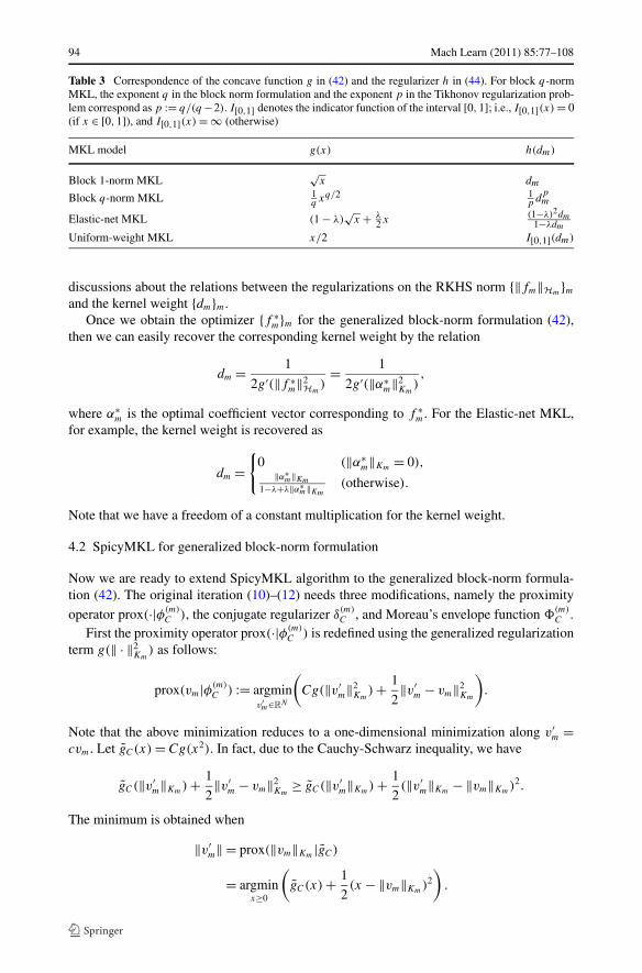
where we define the regularizer h(dm) = −2g∗(1/(2dm)). It is easy to obtain the regularizerh corresponding to the block 1-norm MKL, block q-norm MKL, and the Elastic-net MKL,and it is shown in Table 3. See Tomioka and Suzuki (2011) for more detailed and generalized

94 Mach Learn (2011) 85:77–108

Table 3 Correspondence of the concave function g in (42) and the regularizer h in (44). For block q-normMKL, the exponent q in the block norm formulation and the exponent p in the Tikhonov regularization prob-lem correspond as p := q/(q −2). I[0,1] denotes the indicator function of the interval [0,1]; i.e., I[0,1](x) = 0(if x ∈ [0,1]), and I[0,1](x) = ∞ (otherwise)

MKL model g(x) h(dm)

Block 1-norm MKL√

x dm

Block q-norm MKL 1q xq/2 1

p dpm

Elastic-net MKL (1 − λ)√

x + λ2 x

(1−λ)2dm1−λdm

Uniform-weight MKL x/2 I[0,1](dm)

discussions about the relations between the regularizations on the RKHS norm {‖fm‖Hm}m

and the kernel weight {dm}m.Once we obtain the optimizer {f ∗

m}m for the generalized block-norm formulation (42),then we can easily recover the corresponding kernel weight by the relation

dm = 1

2g′(‖f ∗m‖2

Hm)

= 1

2g′(‖α∗m‖2

Km),

where α∗m is the optimal coefficient vector corresponding to f ∗

m. For the Elastic-net MKL,for example, the kernel weight is recovered as

dm ={

0 (‖α∗m‖Km = 0),

‖α∗m‖Km

1−λ+λ‖α∗m‖Km

(otherwise).

Note that we have a freedom of a constant multiplication for the kernel weight.

4.2 SpicyMKL for generalized block-norm formulation

Now we are ready to extend SpicyMKL algorithm to the generalized block-norm formula-tion (42). The original iteration (10)–(12) needs three modifications, namely the proximity

operator prox(·|φ(m)C ), the conjugate regularizer δ

(m)C , and Moreau’s envelope function �

(m)C .

First the proximity operator prox(·|φ(m)C ) is redefined using the generalized regularization

term g(‖ · ‖2Km

) as follows:

prox(vm|φ(m)C ) := argmin

v′m∈RN

(

Cg(‖v′m‖2

Km) + 1

2‖v′

m − vm‖2Km

)

.

Note that the above minimization reduces to a one-dimensional minimization along v′m =

cvm. Let gC(x) = Cg(x2). In fact, due to the Cauchy-Schwarz inequality, we have

gC(‖v′m‖Km) + 1

2‖v′

m − vm‖2Km

≥ gC(‖v′m‖Km) + 1

2(‖v′

m‖Km − ‖vm‖Km)2.

The minimum is obtained when

‖v′m‖ = prox(‖vm‖Km |gC)

= argminx≥0

(

gC(x) + 1

2(x − ‖vm‖Km)2

)

.

Mach Learn (2011) 85:77–108 95

For example, for Elastic-net MKL, the regularizer g is written as g(x) = (1 − λ)x + λx2/2,and the one dimensional proximity operator prox(·|gC) is obtained as follows:

prox(x|gC) ={

0 (if 0 ≤ x ≤ C(1 − λ)),x−C(1−λ)

Cλ+1 (otherwise).

Therefore, the proximity operator prox(vm|φ(m)C ) is obtained as follows:

prox(vm|φ(m)C ) =

{0 (if ‖vm‖Km ≤ C(1 − λ)),‖vm‖Km−C(1−λ)

(Cλ+1)‖vm‖Kmvm (otherwise).

Second, the convex conjugate of the regularizer δ(m)C is redefined as follows:

δ(m)C (um) := sup

αm∈RN

(〈um,αm〉Km− gC(‖αm‖Km)

)

= supαm∈RN

(‖um‖Km‖αm‖Km − gC(‖αm‖Km))

= g∗C(‖um‖Km). (45)

For example, for the same Elastic-net regularizer, the convex conjugate g∗C(y) is obtained as

follows:

g∗C(y) = sup

x≥0

(

xy − C(1 − λ)x − Cλ

2x2

)

={

0 (if 0 ≤ y ≤ C(1 − λ)),(y−C(1−λ))2

2Cλ(otherwise).

(46)

Third the envelope function �(m)C is redefined in terms of the above new conjugate regu-

larizer δ(m)C as follows:

�(m)C (vm) := min

v′m∈RN

(

g∗C(‖v′

m‖Km) + 1

2‖v′

m − vm‖2Km

)

= minv′m∈RN

(

g∗C(‖v′

m‖Km) + 1

2(‖v′

m‖Km − ‖vm‖Km)2

)

= g∗C(‖vm‖Km),

where we again used Cauchy-Schwarz inequality in the second line, and g∗C is the Moreau’s

envelope function of g∗C as follows:

g∗C(y) = min

y′≥0

(

g∗C(y ′) + 1

2(y ′ − y)2

)

.

96 Mach Learn (2011) 85:77–108

With the above three modifications, the SpicyMKL iteration is rewritten as follows:

ρ(t) := argminρ∈RN

(

L∗(−ρ) + 1

γ (t)

M∑

m=1

g∗C(‖αm + γ (t)ρ‖Km) + 1

2γ (t)

(

b + γ (t)

N∑

i=1

ρi

)2)

,

α(t+1)m = prox

(α(t)

m + γ (t)ρ(t)∣∣∣φ

(m)

γ (t)C

)(m = 1, . . . ,M),

b(t+1) = b(t) + γ (t)

N∑

i=1

ρ(t)i .

(47)

Note that if g∗C(0) = 0 (this is the case if gC(0) = 0), the envelope function g∗

C(·) in (47)becomes zero whenever the norm ‖αm + γ (t)ρ‖Km is zero. Thus the inner objective (47) in-herits the computational advantage provided by sparsity of the 1-norm SpicyMKL presentedin Sect. 3.3. Moreover, the gradient and Hessian of the generalized inner objective (47) canbe computed in a similar manner as (26) and (27).

A generalization to the general loss functions with constraints is also straightforward; weonly need to replace ‖prox(αm + γρ|φ(m)

γC )‖2Km

in (41) (the definition of ϕγ (ρ, ρ;α,b, ξ))

with g∗C(‖αm + γρ‖Km).

Implementation of general loss and regularization Our Matlab implementation is suited togeneral loss and block-norm regularization functions. The code runs under general settingsif one plugs in scripts of the following information: the primal and dual functions of the loss,the gradient and Hessian of the dual loss, the primal and dual of the regularization function,the corresponding proximity operator and the derivative of the proximity operator.

4.3 One step optimization for a regularization function with smooth dual

When the convex conjugate δ(m)C of the regularization term φ

(m)C is smooth (twice differen-

tiable), the optimization needs only one step iteration of the outer loop. We illustrate theoptimization method for smooth dual function in a generalized formulation and show twouseful examples, Elastic-net MKL for λ > 0 and block q-norm MKL for q > 1.

The primal problem (7) is equivalent to the following dual problem by Fenchel’s dualitytheorem (Rockafellar 1970, Theorem 31.2):

maximizeρ∈R

N

1�ρ=0

(

− L∗(−ρ) −M∑

m=1

δ(m)C (ρ)

)

, (48)

where L∗ and δ(m)C are the convex conjugate of L and φ

(m)C . Note that the constraint 1�ρ = 0

is due to the bias term b so that if there is no bias term this constraint is removed. Using theexpression for the convex conjugate δ

(m)C in (45), (48) is rewritten as follows:

maximizeρ∈R

N

1�ρ=0

(

− L∗(−ρ) −M∑

m=1

g∗C(‖ρ‖Km)

)

.

Thus if L∗ and g∗ are differentiable, the optimization problem can be easily solved by gra-dient descent or Newton method with the constraint 1�ρ = 0. By a simple calculation, we

Mach Learn (2011) 85:77–108 97

obtain the gradient and Hessian of the dual regularization term as

∇ρg∗C

(‖ρ‖Km

) = Kmρ

‖ρ‖Km

dg∗C(y)

dy

∣∣∣∣∣y=‖ρ‖Km

, (49)

∇∇�ρ g∗

C

(‖ρ‖Km

) =(

Km

‖ρ‖Km

− Kmρρ�Km

‖ρ‖3Km

)dg∗

C(y)

dy

∣∣∣∣∣y=‖ρ‖Km

+ Kmρρ�Km

‖ρ‖2Km

d2g∗C(y)

dy2

∣∣∣∣∣y=‖ρ‖Km

. (50)

To deal with the constraint 1�ρ = 0, we added a penalty function Cb(1�ρ)2 to the objectivefunction in our numerical experiments with large Cb (in our experiments we used Cb = 105).

The primal optimal solution can be computed from the dual optimal solution as follows.Given the dual optimal solution ρ�, the primal optimal solution α� = (α��

1 , . . . , �M )� and b�

satisfy

Kα� + 1b� = −∇ρL∗(−ρ�),

see Rockafellar (1970, Theorem 31.3). By KKT-condition, there is a real number c such that

∇ρL∗(−ρ�) = −

M∑

m=1

∇ρg∗C(‖ρ‖Km)

∣∣∣ρ=ρ�

+ c1

= −M∑

m=1

Kmρ�

‖ρ�‖Km

dg∗C(y)

dy

∣∣∣∣∣y=‖ρ�‖Km

+ c1.

Therefore the primal optimal solution is given as

α�m = ρ�

‖ρ�‖Km

dg∗C(y)

dy

∣∣∣∣∣y=‖ρ�‖Km

, b� = −c.

When L∗ is not differentiable (e.g., hinge loss), combination of the techniques of thissubsection and Sect. 3.4 can resolve the non-differentiability of L∗.

In the following we give two examples; Elastic-net and the block q-norm regularization(q > 1).

4.3.1 Efficient optimization of Elastic-net MKL

In Elastic-net MKL, the regularization term is gC(x) = C(1 − λ)x + Cλ2 x2. The convex

conjugate of gC is given in (46). Therefore

dg∗C(y)

dy=

{0 (|y| ≤ C(1 − λ)),y−C(1−λ)

Cλ(otherwise),

d2g∗(y)

dy2=

{0 (|y| ≤ C(1 − λ)),

1Cλ

(otherwise).

Substituting the gradient and the Hessian to (49) and (50), we obtain the Newton methodfor the dual of Elastic-net MKL. It should be noted that the gradient and Hessian need to becomputed only on active kernels as in Sect. 3.3, i.e. ∇ρg

∗(‖ρ‖Km) = 0, ∇∇�ρ g∗(‖ρ‖Km) = 0

for all m such that ‖ρ‖Km ≤ C(1 − λ).

98 Mach Learn (2011) 85:77–108

4.3.2 Efficient optimization of block q-norm MKL

When q > 1, block q-norm MKL can be solved in one outer step. The regularization termof the block q-norm MKL is written as gC(x) = C

qxq . By a simple calculation, we obtain

the convex conjugate g∗C as:

g∗C(y) = C1−r 1

ryr ,

where r = q

q−1 . Note that r > 1 when q > 1. Then we have

dg∗(y)

dy= C1−ryr−1,

d2g∗(y)

dy2= C1−r (r − 1)yr−2.

Therefore we can apply the Newton method to the dual of �p-norm MKL using the formu-lae (49) and (50).

5 Relations with the existing methods

We briefly illustrate the relations between our approach and the existing methods. Basicallythe existing methods (such as SILP (Sonnenburg et al. 2006), SimpleMKL (Rakotomamonjyet al. 2008), LevelMKL (Xu et al. 2009), and HessianMKL (Chapelle and Rakotomamonjy2008)) rely on the equation (Micchelli and Pontil 2005):

(M∑

m=1

‖fm‖Hm

)2

= infdm≥0,

∑m dm=1

{M∑

m=1

‖fm‖2Hm

dm

}

.

An advantage of this formulation is that we have a smooth upper bound∑M

m=1‖fm‖2

Hm

dmof

the non-smooth �1 regularization. Moreover (1) says that minimizing this upper bound withrespect to {fm}M

m=1 under the constraint f = ∑M

m=1 fm for a given function f , the upperbound becomes the RKHS norm of the function f in the RKHS Hk(d) corresponding to the

averaged kernel k(d) = ∑M

m=1 dmkm, i.e.,

‖f ‖2Hk(d)

= inff =∑M

m=1 fm

{M∑

m=1

‖fm‖2Hm

dm

}

(see Aronszajn 1950 for the proof). Thus we don’t need to consider M functions {fm}Mm=1,

instead we only need to deal with one function f on the averaged kernel function k(d). Thatis, the MKL learning scheme can be converted to

inff1∈H1,...,fM∈HM

N∑

i=1

�

(

yi,

M∑

m=1

fm(xi)

)

+ C

(M∑

m=1

‖fm‖Hm

)2

= infdm≥0,

∑m dm=1

{

inff ∈Hk(d)

N∑

i=1

� (yi, f (xi)) + C‖f ‖2Hk(d)

}

.

One notes that fixing {dm}Mm=1 the problem of the inner minimization is a standard single

kernel learning. Thus the inner minimization is easily solved by using publicly available

Mach Learn (2011) 85:77–108 99

efficient solvers for a single kernel learning. Based on these relations, the existing methodsconsist of the following two parts, the single kernel learning part and the updating part of{dm}m:

1. Minimize L(Kα) + Cα�Kα where K = ∑M

m=1 dmKm.2. Update {dm}M

m=1 so that the objective function decreases,

where the update step differs depending on methods.On the other hand, our approach is totally different from the existing approaches. We

don’t utilize the kernel weight to obtain a smoothed approximation of the objective prob-lem. Our approach utilize the proximal minimization update (8) that can be interpreted as agradient descent of the Moreau’s envelope of the objective function. In general, for a convexfunction f , the Moreau’s envelope f defined below is differentiable:

f (x) := miny

{

f (y) + 1

2γ‖y − x‖2

}

,

∇f (x) = 1

γ(x − y∗(x)) ∈ ∇f (y∗(x))

where y∗(x) = arg miny

{

f (y) + 1

2γ‖y − x‖2

}

.

(51)

One can check that min f = minf and arg min f = arg minf because f (x∗) ≤ f (y∗(x∗))+1

2γ‖y∗(x∗) − x∗‖2 = f (x∗) ≤ f (x∗) + 1

2γ‖x∗ − x∗‖2 = f (x∗) for all x and x∗ ∈ arg minf ,

and if x /∈ arg minf , we have f (x∗) < f (x). Thus the minimization of f leads to the min-imization of f . Using the relation (51), the proximal minimization update (8) correspondsto

x(t+1) ← y∗(x(t)) = x(t) − γ∇f (x(t)) ∈ x(t) − γ∇f (x(t+1)).

Therefore the updating rule is a gradient descent of the Moreau’s envelope of the objec-tive function (and the increment is also the subgradient of f at the next solution x(t+1)).Fortunately the minimization required to obtain the Moreau’s envelope is obtained by asmooth optimization procedure as described in Sect. 3.3. More general and detailed discus-sions about the use of the Moreau’s envelope for machine learning settings can be found inTomioka et al. (2011).

Regarding the optimization of block q-norm MKL, Kloft et al. (2010) considered a uni-fying regularization including block q-norm MKL where the regularization term is

C1

(M∑

m=1

‖fm‖qHm

) 2q

+ C2

M∑

m=1

‖fm‖2Hm

,

(there is additional operation (·) 2q at the q-norm term compared with our block q-norm

MKL formulation, however there is one-to-one correspondence between both formulationsas in the same reason described in the end of Sect. 2.2). They also noticed that the dualof the above unifying regularization is smooth unless C2 = 0 and q = 1, and suggest toutilize L-BFGS to solve the dual problem. This corresponds to the special case of our settingg(x) = (1 − λ)xq/2 + λx with 0 ≤ λ ≤ 1. As shown in Sect. 4.3, we can solve the MKLproblem with this regularization by one step outer iteration because of the smoothness of itsdual.

100 Mach Learn (2011) 85:77–108

6 Numerical experiments

In this section, we experimentally confirm the efficiency of the proposed SpicyMKL on sev-eral binary classification tasks from UCI and IDA machine learning repository.5 We com-pared our algorithm SpicyMKL to four state-of-the-art algorithms namely SILP (Sonnen-burg et al. 2006), SimpleMKL (Rakotomamonjy et al. 2008), LevelMKL (Xu et al. 2009)and HessianMKL (Chapelle and Rakotomamonjy 2008). As for SpicyMKL, we report theresults of hinge and logistic losses with block 1-norm regularization. We also report the re-sult of the one step optimization method for elastic-net regularization (the method describedin Sect. 4.3.1) with hinge and logistic losses. To distinguish the iterative method and theone step method, we call the one step optimization method for elastic-net regularization asElastMKL.

6.1 Performances on UCI benchmark datasets

We used 5 datasets from the UCI repository (Asuncion and Newman 2007): ‘Liver’, ‘Pima’,‘Ionospher’, ‘Wpbc’, ‘Sonar’. The candidate kernels were Gaussian kernels with 24 differentbandwidths (0.1 0.25 0.5 0.75 1 2 3 4 . . . 19 20) and polynomial kernels of degree 1 to 3.All of 27 different kernel functions (24 Gaussian kernels and 3 polynomial kernels) wereapplied to individual variables as well as jointly over all the variables; i.e., in total we have27× (n+1) candidate kernels, where n is the number of variables. All kernel matrices werenormalized to unit trace (Km ← Km/trace(Km)), and were precomputed prior to running thealgorithms. These experimental settings were borrowed from the paper (Rakotomamonjy etal. 2008) of SimpleMKL, but we used a larger number of kernels.

For each dataset, we randomly chose 80% of samples for training and the remaining20% for testing. This procedure was repeated 10 times. Experiments were run on 3 differ-ent regularization parameters C = 0.005, 0.05 and 0.5; for SimpleMKL, LevelMKL andHessianMKL, the regularization parameter was converted by (6). We employed the relativeduality gap, (primal obj − dual obj)/primal obj with tolerance 0.01 as the stopping criterionfor all algorithms. The primal objective for SpicyMKL and ElastMKL can be computed byusing α(t) and b(t). In order to compute the dual objective of SpicyMKL and ElastMKL,we project the multiplier vector ρ to the equality constraint ρ = ρ − 1(

∑ρi)/N and in

addition, for SpicyMKL with block 1-norm regularization, we project ρ to the domain ofδ

(m)C (21) by ρ ′ = ρ/max{maxm{‖ρ‖Km/C},1}. Then we compute the dual objective func-

tion as −L∗(−ρ). The same technique can be found in Tomioka and Sugiyama (2009) andWright et al. (2009). The primal objective of SILP, SimpleMKL, HessianMKL and Lev-elMKL is computed as

∑i αi − 1

2

∑i,j αiαj

∑m dmKm(xi, xj ) and the dual objective as

∑i αi − 1

2 maxm

∑i,j αiαjKm(xi, xj ) where αi is the dual variable of SVM solved at each

iteration and dm is the kernel weight (see Sonnenburg et al. 2006 and Rakotomamonjy et al.2008).

For SpicyMKL and ElastMKL, we report the result from two loss functions; the hingeloss and the logistic loss. We used λ = 0.5 for ElastMKL. For SILP, SimpleMKL, Lev-elMKL and HessianMKL, we used the hinge loss. For SILP, we used Shogun implementa-

5All the experiments were executed on Intel Xeon 3.33 GHz with 48 GB RAM.

Mach Learn (2011) 85:77–108 101

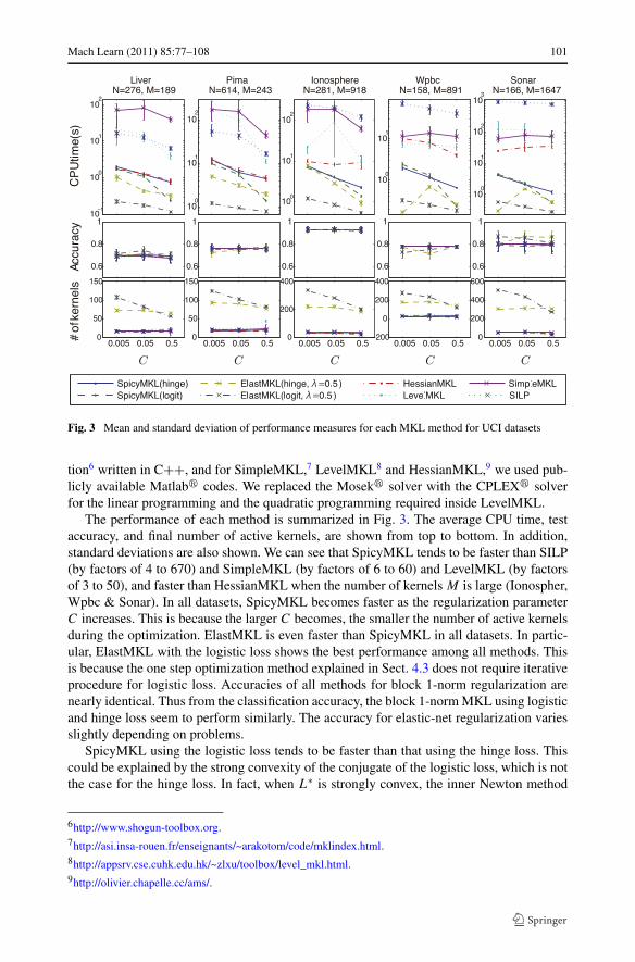
Fig. 3 Mean and standard deviation of performance measures for each MKL method for UCI datasets

tion6 written in C++, and for SimpleMKL,7 LevelMKL8 and HessianMKL,9 we used pub-licly available Matlab� codes. We replaced the Mosek� solver with the CPLEX� solverfor the linear programming and the quadratic programming required inside LevelMKL.

The performance of each method is summarized in Fig. 3. The average CPU time, testaccuracy, and final number of active kernels, are shown from top to bottom. In addition,standard deviations are also shown. We can see that SpicyMKL tends to be faster than SILP(by factors of 4 to 670) and SimpleMKL (by factors of 6 to 60) and LevelMKL (by factorsof 3 to 50), and faster than HessianMKL when the number of kernels M is large (Ionospher,Wpbc & Sonar). In all datasets, SpicyMKL becomes faster as the regularization parameterC increases. This is because the larger C becomes, the smaller the number of active kernelsduring the optimization. ElastMKL is even faster than SpicyMKL in all datasets. In partic-ular, ElastMKL with the logistic loss shows the best performance among all methods. Thisis because the one step optimization method explained in Sect. 4.3 does not require iterativeprocedure for logistic loss. Accuracies of all methods for block 1-norm regularization arenearly identical. Thus from the classification accuracy, the block 1-norm MKL using logisticand hinge loss seem to perform similarly. The accuracy for elastic-net regularization variesslightly depending on problems.

SpicyMKL using the logistic loss tends to be faster than that using the hinge loss. Thiscould be explained by the strong convexity of the conjugate of the logistic loss, which is notthe case for the hinge loss. In fact, when L∗ is strongly convex, the inner Newton method

6http://www.shogun-toolbox.org.7http://asi.insa-rouen.fr/enseignants/~arakotom/code/mklindex.html.8http://appsrv.cse.cuhk.edu.hk/~zlxu/toolbox/level_mkl.html.9http://olivier.chapelle.cc/ams/.

102 Mach Learn (2011) 85:77–108

Table 4 Average number of outer iterations. Average number of SVM evaluations is also shown in the bracefor SimpleMKL

Dataset C Spicy Spicy Simple Hessian Level SILP

(hinge) (logit)

Liver 0.005 22.6 20.1 200.3(3770.2) 13.2 171.6 718.8

0.05 14.1 14.5 222.2(4800.0) 11.8 138.0 517.2

0.5 6.7 3.3 134.2(2200.5) 9.4 50.1 237.8

Pima 0.005 31.5 21.5 76.2(1488.9) 15.4 290.7 1020.1

0.05 13.6 13.9 74.9(1511.7) 12.2 197.9 727.1

0.5 7.9 3.2 24.6(470.9) 10.2 30.9 258.0

Ionosphere 0.005 38.0 24.6 184.5(2864.1) 11.3 100.9 1810.3

0.05 18.3 17.1 188.6(2983.1) 10.3 135.6 1580.1

0.5 7.8 5.4 57.8(1374.4) 14.4 65.5 972.0

Wpbc 0.005 24.0 24.4 45.4(1014.2) 11.6 61.3 683.6

0.05 13.2 14.4 49.1(1134.7) 10.7 60.8 514.2

0.5 6.0 2.0 40.9(964.4) 7.2 55.4 367.0

Sonar 0.005 35.2 27.2 158.3(2736.8) 10.3 193.0 4484.6

0.05 16.6 16.8 204.8(3535.3) 10.6 194.2 4356.4

0.5 7.7 4.2 173.3(3511.4) 19.6 154.4 3862.3

(minimization of ϕγ with respect to ρ) converges rapidly. Although the logistic loss is oftenfaster to train, yet the accuracy is nearly identical to that of the hinge loss.

When the regularization is elastic-net, the hinge loss gives sparser solution than the logis-tic loss. The number of kernels selected under elastic-net regularization is much lager thanthat under block 1-norm regularization as expected, and decreases as the strength of regu-larization C increases. Under block 1-norm regularization, the number of kernels slightlydecreases as C increases.

In Table 4, a comparison of the average numbers of outer iterations and SVM evalu-ations on the UCI datasets is reported. The existing methods (HessianMKL, LevelMKL,SimpleMKL, SILP) iterate the update of the kernel weight {dm}M

m=1 and the SVM evalua-tion of the objective function at the current weight as illustrated in Sect. 5. We refer to thecombination of these two steps as one outer iteration. Since SimpleMKL requires severalSVM evaluations during the line search in gradient descent, the number of outer iterationsand that of SVM evaluations are different. As for the other methods, both quantities aresame. Obviously ElastMKL requires only one outer iteration, thus the result for ElastMKLis not reported in the table. We can see that in all methods the number of outer iterationsdecreases as the regularization parameter C increases. This is because as the regularizationbecomes strong, the required number of kernels becomes small and accordingly the intrinsicproblem size becomes small. SpicyMKL and HessianMKL require much smaller number ofiterations than others. This shows that these methods have fast convergence rate and thusthe solution drastically approaches to the optimal one at each iteration. Comparing the CPUtime required by SpicyMKL and HessianMKL, SpicyMKL tends to require light computa-tion per iteration especially for large number of kernels while HessianMKL requires QP toderive the update direction that is heavy for large number of kernels.

Mach Learn (2011) 85:77–108 103

Fig. 4 Duality gap and # of active kernels against CPU time

In Fig. 4(a), we plot the relative duality gaps against CPU time for a single run ofSpicyMKL (with logistic loss and block 1-norm regularization), HessianMKL, LevelMKLand SimpleMKL on the ‘Wpbc’ dataset. We can see that the duality gap of SpicyMKLdrops rapidly and it is faster than linear. That supports the super-linear convergence of ourmethod. HessianMKL decreases the duality gap quickly because HessianMKL is a secondorder method. The duality gap of LevelMKL gradually drops in the early stage, but afterseveral steps, the behavior of duality gap becomes unstable. After all, the duality gap ofLevelMKL did not drop below 10−2 in 500 iteration steps. This is because the size of QPrequired in LevelMKL increases as the algorithm proceeds so that it gets hard to obtain aprecise solution. SILP shows fluctuations of the duality gap so that the duality gap does notdecrease monotonically. This is because the sequence of the solutions generated by cuttingplane method shows oscillation behavior. Figure 4(b) shows the number of active kernels asa function of the CPU time spent by the algorithm. Here we again observe rapid decreasein the number of kernels for SpicyMKL. This reduces huge amount of computation per it-eration. We see a relation between the speed of convergence and the number of kernels inSpicyMKL; as the number of kernels decreases, the time spent per iteration becomes small.

6.2 Scaling against the sample size and the number of kernels

Here we investigate the dependency of CPU time on the number of kernels and the samplesize. We used 4 datasets from IDA benchmark repository (Rätsch et al. 2001): ‘Ringnorm’,‘Splice’, ‘Twonorm’ and ‘Waveform’. The same relative duality gap criterion with tolerance0.01 was used. We generated a set of basis kernels by randomly selecting subsets of featuresand applying Gaussian kernels with random width σ = 5χ2 +0.1, where χ2 is a chi-squaredrandom variable. Here we report ElastMKL with λ = 0.1,0.5 with hinge and logistic lossin addition to SpicyMKL with block 1-norm regularization with hinge and logistic loss,SimpleMKL, HessianMKL, LevelMKL and SILP.

In Fig. 5, the number of kernels is increased from 50 to 6000. The graph shows the me-dian of CPU times with 25 and 75 percentiles over 10 random train-test splitting wherethe size of training set was fixed to 200. We observe that for small number of kernels theCPU time of HessianMKL is the fastest among all methods with block 1-norm regulariza-tion. However when the number of kernels is greater than 1000, our method SpicyMKL isclearly the fastest among the methods with block 1-norm regularization. In fact, SpicyMKL

104 Mach Learn (2011) 85:77–108

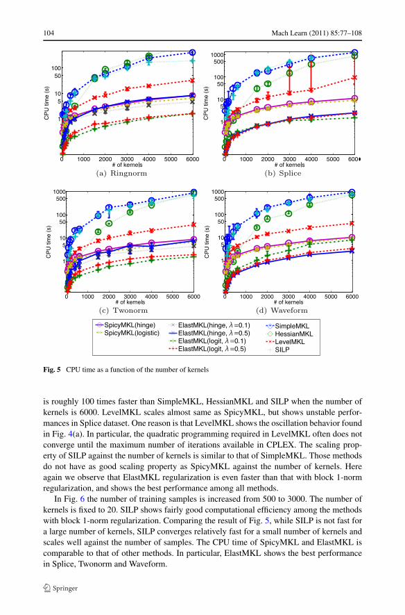
Fig. 5 CPU time as a function of the number of kernels

is roughly 100 times faster than SimpleMKL, HessianMKL and SILP when the number ofkernels is 6000. LevelMKL scales almost same as SpicyMKL, but shows unstable perfor-mances in Splice dataset. One reason is that LevelMKL shows the oscillation behavior foundin Fig. 4(a). In particular, the quadratic programming required in LevelMKL often does notconverge until the maximum number of iterations available in CPLEX. The scaling prop-erty of SILP against the number of kernels is similar to that of SimpleMKL. Those methodsdo not have as good scaling property as SpicyMKL against the number of kernels. Hereagain we observe that ElastMKL regularization is even faster than that with block 1-normregularization, and shows the best performance among all methods.

In Fig. 6 the number of training samples is increased from 500 to 3000. The number ofkernels is fixed to 20. SILP shows fairly good computational efficiency among the methodswith block 1-norm regularization. Comparing the result of Fig. 5, while SILP is not fast fora large number of kernels, SILP converges relatively fast for a small number of kernels andscales well against the number of samples. The CPU time of SpicyMKL and ElastMKL iscomparable to that of other methods. In particular, ElastMKL shows the best performancein Splice, Twonorm and Waveform.

Mach Learn (2011) 85:77–108 105

Fig. 6 CPU time as a function of the sample size

7 Conclusion and future direction

In this article, we have proposed a new efficient training algorithm for MKL with generalconvex loss functions and general regularizations. The proposed SpicyMKL algorithm gen-erates a sequence of primal variables by iteratively optimizing a sequence of smooth min-imization problems. The outer loop of SpicyMKL is a proximal minimization method andit converges super-linearly. The inner minimization is efficiently carried out by the New-ton method. We introduced a generalized block norm formulation of MKL regularizationthat includes non-sparse regularizations such as Elastic-net MKL and block q-norm MKL,and derived the connections between our block norm formulation and the kernel weights.Then we derived a general optimization method that is applicable to the general block normframework. We also gave an efficient one step optimization method for regularizations withsmooth dual (e.g., elastic-net and block q-norm).

We have shown through numerical experiments that SpicyMKL scales well with increas-ing number of kernels and it has similar scaling behavior against the number of samples toconventional methods. It is worth noting that SpicyMKL does not rely on solving LP or QPproblems, which itself can be a challenging task; accordingly SpicyMKL can reliably obtain

106 Mach Learn (2011) 85:77–108

a precise solution. SpicyMKL with the logistic loss and elastic-net regularization has shownthe best performance while showing fairly good accuracies.

Future work includes a second order modification of the update rule of the primal vari-ables, and combination of the techniques developed in SpicyMKL and wrapper methods(Sonnenburg et al. 2006; Rakotomamonjy et al. 2008; Chapelle and Rakotomamonjy 2008).

It would also be interesting to develop an efficient decomposition method to deal with alarge sample size problem. Since the dual problem (25) of the inner loop is an N dimensionaloptimization problem, when the number of samples N is large, the naive Newton methodor other gradient descent type methods might be hard to be applied. In such a situation, theblock-coordinate descent algorithm might be useful. That is, decompose N variables {ρi}N

i=1into some groups (say B groups {ρIi }B

i=1) and iteratively minimize the objective functionwith respect to one group with other groups fixed:

ρk+1Ii

← arg minρIi

ϕγ (t) ((ρk+1I1

, . . . , ρk+1Ii−1

, ρIi , ρkIi+1

, . . . , ρkIB

);α(t), b(t))

(see Sect. 5.4.3 of Zangwill 1969 and Proposition 2.7.1 of Bertsekas 1999). In a similarsense, Sequential Minimal Optimization (SMO) algorithm (Platt 1999) might be useful forsome loss function classes such as the hinge loss. We leave these important issues for futurework.

Acknowledgements We would like to thank anonymous reviewers for their constructive comments, whichimproved the quality of this paper. We would also like to thank Manik Varma, Marius Kloft, AlexanderZien, and Cheng Soon Ong for helpful discussions. This work was partially supported by MEXT KAKENHI22700289 and 22700138.

Appendix: Proof of Theorem 1

Combining (15), (19), and (24), we can rewrite the dual of the proximal MKL problem (8)as follows:

minimizeρ∈R

N

u∈RMN

{

L∗(−ρ) +M∑

m=1

δ(m)C (um)

+M∑

m=1

(

α(t)m

�Km(ρ − um) + γ (t)

2‖ρ − um‖2

Km

)

+ b(t)1�ρ − γ (t)

2

(1�ρ

)2}

,

where the maximization is turned into minimization and we redefined um/γ (t) as um. Thisformulation is known as the augmented Lagrangian for the dual of the MKL optimizationproblem (7), which can be expressed as follows:

minimizeρ∈R

N ,

u∈RMN

L∗(−ρ) +M∑

m=1

δ(m)C (um),

subject to K1/2m (ρ − um) = 0 (m = 1, . . . ,M),

1�ρ = 0.

Mach Learn (2011) 85:77–108 107

K1/2m α(t)

m and b(t) are the Lagrangian multipliers corresponding to the above M + 1 equalityconstraints (Hestenes 1969; Powell 1969; Tomioka and Sugiyama 2009). We apply Propo-sition 5.11 of Bertsekas (1982) so that we obtain

M∑

m=1

‖α(t)m − α∗

m‖2Km

+ (b(t) − b∗)2 → 0 (as t → ∞).

Thus there is sufficiently large T such that for all t ≥ T , (α(t), b(t)) is inside the δ-neighborhood of (α∗, b∗). Therefore we can assume that (9) holds at (α(t), b(t)) for all t ≥ T .Finally Theorem 3 of Tomioka et al. (2011) (and its proof) gives the assertion (see also theproof of Proposition 5.22 of Bertsekas 1982 where φ(t) = t2 and ∇φ(t) = t are substitutedfor our setting).

References

Aronszajn, N. (1950). Theory of reproducing kernels. Transactions of the American Mathematical Society,68, 337–404.

Asuncion, A., & Newman, D. (2007). UCI machine learning repository. http://www.ics.uci.edu/~mlearn/MLRepository.html.

Bach, F. R. (2008). Consistency of the group Lasso and multiple kernel learning. Journal of Machine LearningResearch, 9, 1179–1225.

Bach, F. R., Lanckriet, G., & Jordan, M. (2004). Multiple kernel learning, conic duality, and the SMO algo-rithm. In Proceedings of the 21st international conference on machine learning (pp. 41–48).

Bach, F. R., Thibaux, R., & Jordan, M. I. (2005). Computing regularization paths for learning multiple ker-nels. In Advances in neural information processing systems (Vol. 17, pp. 73–80). Cambridge: MITPress.

Bertsekas, D. P. (1982). Constrained optimization and Lagrange multiplier methods. New York: AcademicPress.

Bertsekas, D. P. (1999). Nonlinear programming. Nashua: Athena Scientific.Candes, E. J., Romberg, J., & Tao, T. (2006). Robust uncertainty principles: Exact signal reconstruction from

highly incomplete frequency information. IEEE Transactions on Information Theory, 52(2), 489–509.Chapelle, O., & Rakotomamonjy, A. (2008). Second order optimization of kernel parameters. In NIPS work-

shop on kernel learning: automatic selection of optimal kernels, Whistler.Cortes, C. (2009). Can learning kernels help performance? Invited talk at International Conference on Ma-

chine Learning (ICML 2009), Montréal, Canada.Cortes, C., Mohri, M., & Rostamizadeh, A. (2009). L2 regularization for learning kernels. In Proceedings of

the 25th conference on uncertainty in artificial intelligence (UAI 2009), Montréal, Canada.Daubechies, I., Defrise, M., & Mol, C. D. (2004). An iterative thresholding algorithm for linear inverse

problems with a sparsity constraint. Communications on Pure and Applied Mathematics, LVII, 1413–1457.

Figueiredo, M., & Nowak, R. (2003). An EM algorithm for wavelet-based image restoration. IEEE Transac-tions on Image Processing, 12, 906–916.

Gehler, P. V., & Nowozin, S. (2009). Let the kernel figure it out; principled learning of pre-processing forkernel classifiers. In Proceedings of the IEEE computer society conference on computer vision andpattern (CVPR2009).

Hestenes, M. (1969). Multiplier and gradient methods. Journal of Optimization Theory and Applications, 4,303–320.

Kimeldorf, G. S., & Wahba, G. (1971). Some results on Tchebycheffian spline functions. Journal of Mathe-matical Analysis and Applications, 33, 82–95.

Kloft, M., Brefeld, U., Sonnenburg, S., Laskov, P., Müller, K. R., & Zien, A. (2009). Efficient and accurate �p -norm multiple kernel learning. In Y. Bengio, D. Schuurmans, J. Lafferty, C. K. I. Williams, & A. Culotta(Eds.), Advances in neural information processing systems (Vol. 22, pp. 997–1005). Cambridge: MITPress.

Kloft, M., Rückert, U., & Bartlett, P. L. (2010). A unifying view of multiple kernel learning. arXiv:1005.0437.Lanckriet, G., Cristianini, N., Ghaoui, L. E., Bartlett, P., & Jordan, M. (2004). Learning the kernel matrix

with semi-definite programming. Journal of Machine Learning Research, 5, 27–72.

108 Mach Learn (2011) 85:77–108

Micchelli, C. A., & Pontil, M. (2005). Learning the kernel function via regularization. Journal of MachineLearning Research, 6, 1099–1125.

Mosci, S., Santoro, M., Verri, A., & Villa, S. (2008). A new algorithm to learn an optimal kernel basedon Fenchel duality. In NIPS 2008 workshop: kernel learning: automatic selection of optimal kernels,Whistler.

Nath, J. S., Dinesh, G., Raman, S., Bhattacharyya, C., Ben-Tal, A., & Ramakrishnan, K. R. (2009). On thealgorithmics and applications of a mixed-norm based kernel learning formulation. In Advances in neuralinformation processing systems (Vol. 22, pp. 844–852). Cambridge: MIT Press.

Palmer, J., Wipf, D., Kreutz-Delgado, K., & Rao, B. (2006). Variational EM algorithms for non-Gaussianlatent variable models. In Y. Weiss, B. Schölkopf, & J. Platt (Eds.), Advances in neural informationprocessing systems (Vol. 18, pp. 1059–1066). Cambridge: MIT Press.

Platt, J. C. (1999). Using sparseness and analytic QP to speed training of support vector machines. In Ad-vances in neural information processing systems (Vol. 11, pp. 557–563). Cambridge: MIT Press.

Powell, M. (1969). A method for nonlinear constraints in minimization problems. In R. Fletcher (Ed.), Opti-mization (pp. 283–298). London: Academic Press.

Rakotomamonjy, A., Bach, F., & Canu, S. Y. G. (2008). SimpleMKL. Journal of Machine Learning Research,9, 2491–2521.

Rätsch, G., Onoda, T., & Müller, K. R. (2001). Soft margins for adaboost. Machine Learning, 42(3), 287–320.

Rockafellar, R. T. (1970). Convex analysis. Princeton: Princeton University Press.Rockafellar, R. T. (1976). Augmented Lagrangians and applications of the proximal point algorithm in convex

programming. Mathematics of Operations Research, 1, 97–116.Schölkopf, B., & Smola, A. J. (2002). Learning with kernels. Cambridge: MIT Press.Sonnenburg, S., Rätsch, G., Schäfer, C., & Schölkopf, B. (2006). Large scale multiple kernel learning. Journal

of Machine Learning Research, 7, 1531–1565.Tomioka, R., & Sugiyama, M. (2009). Dual augmented lagrangian method for efficient sparse reconstruction.

IEEE Signal Processing Letters, 16(12), 1067–1070.Tomioka, R., & Suzuki, T. (2009). Sparsity-accuracy trade-off in MKL. arXiv:1001.2615.Tomioka, R., & Suzuki, T. (2011). Regularization strategies and empirical Bayesian learning for MKL.

arXiv:1011.3090.Tomioka, R., Suzuki, T., & Sugiyama, M. (2011). Super-linear convergence of dual augmented lagrangian

algorithm for sparse learning. Journal of Machine Learning Research, 12, 1501–1550.Wright, S. J., Nowak, R. D., & Figueiredo, M. A. T. (2009). Sparse reconstruction by separable approxima-

tion. IEEE Transactions on Signal Processing, 57(7), 2479–2493. doi:10.1109/TSP.2009.2016892.Xu, Z., Jin, R., King, I., & Lyu, M. R. (2009). An extended level method for efficient multiple kernel learning.

In Advances in neural information processing systems (Vol. 21, pp. 1825–1832). Cambridge: MIT Press.Yuan, M., & Lin, Y. (2006). Model selection and estimation in regression with grouped variables. Journal of

the Royal Statistical Society, Series B, 68(1), 49–67.Zangwill, W. I. (1969). Nonlinear programming: a unified approach. New York: Prentice Hall.Zien, A., & Ong, C. (2007). Multiclass multiple kernel learning. In Proceedings of the 24th international

conference on machine learning (pp. 11910–1198). New York: ACM.