spike sorting: what is it? why do we need it? where does it come from? how is it done? how to...

Spike sorting: What is it? Why do weneed it? Where does it come from? How

is it done? How to interpret it?III. Improving sorting quality throughstochastic modeling of spike trains.

Christophe PouzatMathématiques Appliquées à Paris 5 (MAP5)

Université Paris-Descartes and CNRS UMR 8145

[email protected]

Thursday November 27, 2014

Where are we ?

What makes data "difficult"

An interlude to keep you motivated

A more realistic model and its problems

A analogy with statistical physics

Back to our simulated data

Application to real data

Yesterday’s summary

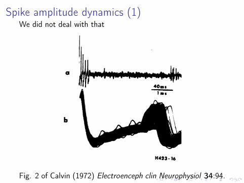
Spike amplitude dynamics (1)We did not deal with that

Fig. 2 of Calvin (1972) Electroenceph clin Neurophysiol 34:94.

Spike amplitude dynamics (2)

Fig. 3 of Pouzat (2005) Technique(s) for Spike Sorting. InMethods and Models in Neurophysics. Les Houches 2003.Elsevier.

Spike amplitude dynamics (3)

We try a naive "exponential relaxation model" for these data:

a (isi) = p · (1− δ · exp (−λ · isi)) .

The exponential relaxation in only anapproximation!

Fig. 3A of Delescluse and Pouzat (2006) J Neurosci Methods150:16.

Neuronal discharges are not Poisson

Fig. 7 of Kuffler, Fitzhugh and Barlow (1957) J Gen Physiol40:683. Evidence for serial correlation of the intervals wasfound (p 687). Hagiwara (1950, 1954) made similar reports.

Log-normal density

Empirical ISI densities are better described by a log-normaldensity than by a Poisson density:

πISI (ISI = isi) =1

isi f√2π

exp

[−12

(ln isi − ln s

f

)2]

where, s is a scale parameter (measured in sec) and f is adimensionless shape parameter.

Log-normal density: exemples

What do we want?

I Recognizing that the inter spike interval (ISI) distribution,and more generally the neuron’s stochastic intensity,provides potentially useful information for spike sorting,we would like a data generation model including thisinformation.

I We would also like a data generation model giving roomfor a description of the spikes amplitude dynamics duringbursts.

Where are we ?







Some simulated data

Simulated data with 3 neurones on 2 recording sites.

The results we will get

Where are we ?







First "improved" model

We will assume that the neuron discharge independently andthat:

I Individual discharges are well approximated by a renewalprocess with a log-normal density.

I The spike amplitude depends on the elapsed time sincethe last spike (of the same neuron); this dependence ismoreover well approximated by an exponential relaxation.

I The recording noise is white and Gaussian and isindependent of the spikes.

Likelihood for single neuron data (1)

We have:

π (D | p, δ, λ, s, f ) =N∏j=1

πisi (ij | s, f ) · πamp (aj | ij ,p, δ, λ) ,

where

πamp (aj | ij ,p, δ, λ) =1

(2π)ns2· e−

12‖aj−p·(1−δ·exp(−λ·ij))‖2

.

Likelihood for single neuron data (2)

The log-likelihood can be written as the sum of two terms:

L (D | p, δ, λ, s, f ) = Lisi (D | s, f ) + Lamp (D | p, δ, λ )

where:

Lisi (D | s, f ) = −N · ln f −N∑j=1

ln ij +12

ln(

ijs

)f

2+Cst

and:

Lamp (D | p, δ, λ ) = −12

N∑j=1

‖aj − p · (1− δ · exp (−λ · ij))‖2+Cst .

Configuration

We will use Θ for our model parameters vector, that is, for amodel with K neurons:

Θ = (P1,∆1,Λ1, S1,F1, . . . ,PK ,∆K ,ΛK , SK ,FK ) .

We will formalize our a priori ignorance of the origin of eachspike by associating to each spike, j , a label Lj ∈ {1, . . . ,K}.lj = 3 means that event j was generated by neuron 3.We will use C for the configuration, that is, the randomvariable:

C = (L1, . . . , LN)T .

With this formalism, spike sorting amounts to estimating theconfiguration.

Likelihood for data from several neurons

If the configuration realization is known, the likelihoodcomputation is easily done:

π (D | c , θ) =K∏

q=1

Nq∏j=1

πisi (iq,j | sq, fq)·πamp

(aq,j | iq,j ,pq, δq, λq

).

Bayesian formalism (1)I Being somewhat opportunist, we are going to formalize

our ignorance on the configuration c and the modelparameters θ by viewing them as realizations of therandom variables C and Θ.

I We then have a triplet of random variables D (whoserealization is D), C and Θ.

I We have, by definition of the conditional probability:

π(D, c , θ) = π(c , θ | D)π(D) = π(D | c , θ) π(c , θ) .

I Rearranging the last two members we get (Bayes rule orBayes "theorem"):

π(c , θ | D) =π(D | c , θ) π(c , θ)

π(D).

Bayesian formalism (2)

I In the literature, our π(c , θ) is called the a priori densityand is written πprior (c , θ); that’s what we know about theparameters and configuration before observing the data.

I Our π(c , θ | D) is called the a posteriori density and iswritten πposterior (c , θ | D); that’s what we know about theparameters and configuration after observing the data.

I Bayes rule tells us how to update our knowledge once thedata have been observed.

I We know how to compute the "likelihood" π(D | c , θ).

Bayesian formalism (3)I We will write πprior (c , θ) = πprior (c)πprior (θ) and takeπprior (c) uniform on C = {1, . . . ,K}N (notice that I’mcheating, I can know N only after seeing the data) andtake

πprior (θ) =K∏

q=1

πprior (sq)πprior (fq)πprior (pq)πprior (δq)πprior (λq) ,

and each of the terms is going to be the density of auniform distribution over a large domain.

I The real problem is the denominator:

π(D) =∑c∈C

∫θ

π(D, c , θ)dθ =∑c∈C

∫θ

π(D | c , θ)πprior (c , θ)dθ ,

since it involves a summation over KN configurations andK is of the order of 10 and N of the order of 1000!

Bayesian formalism (4)I Assuming we find a way to circumvent the "combinatorial

explosion" (KN) problem and to get an estimator,π(c , θ | D), of:

πposterior (c , θ | D) =π(D | c , θ) π(c , θ)

π(D).

I The estimated posterior configuration probability wouldbe:

πposterior (c | D) =

∫θ

π(c , θ | D)dθ .

I The spike sorting results could then be summarized by theMaximum A Posteriori (MAP) estimator:

c = argminc∈C

πposterior (c | D) .

Bayesian formalism (5)

I Clearly, a better use of the results would be for anystatistics T (C ) (think of the cross-correlogram betweentwo spike trains) to use:

T (C ) =∑c∈C

T (c)πposterior (c | D) ,

instead of: T (c).I But to do all that we have to deal with the combinatorial

explosion!I In such situations, a "good strategy" is too look at other

domains to see if other people met a similar problem andfound a solution. . .

Where are we ?







A analogy with statistical physics (1)I Luckily for us, Physicists got a problem similar to ours at

the turn of the 1950s and found a solution.I Let us write:

E (c , θ | D) = − log [π (D | c , θ) · πprior (c , θ)] ,

notice that we know how to compute E (c , θ | D).I Then:

πposterior (c , θ | D) =exp [−βE (c , θ | D)]

π(D),

where β = 1, β is the inverse temperature for Physicistswho write Z (β) = π(D) and call it the partition function.

I Written in this way, πposterior (c , θ | D), is nothing morethan a Gibbs distribution.

A analogy with statistical physics (2)

I Physicists don’t know how to compute the partitionfunction Z (β) in many cases of interest.

I But they need to compute quantities like:∑c∈C

∫θ

T (c , θ)πposterior (c , θ | D)dθ .

I In 1953, Metropolis, Rosenbluth, Rosenbluth, Teller andTeller published "Equation of State Calculations by FastComputing Machines" in Journal of Chemical Physics,proposing an algorithm for estimating this kind of integralwithout knowing the partition function.

A analogy with statistical physics (3)

I In 1971, Hastings published "Monte Carlo SamplingMethods Using Markov Chains and Their Applications" inBiometrika proving that the previous algorithm wasindeed doing what it was suppose to do.

I This algorithm is know called the Metropolis-HastingsAlgorithm.

Metropolis-Hastings in a simple setting (1)

I We will generate a collection of states{x (1), x (2), . . . , x (R)} according to a target distributionπ(x) (the x stand here for our previous c , θ).

I To that end we use a Markov chain which asymptoticallyreaches the stationary distribution π(x).

I A Markov chain is uniquely defined by its transitionmatrix P(X (k+1) = x ′ | X (k) = x) and its initial statedistribution.

Metropolis-Hastings in a simple setting (2)I A Markov chain has a unique stationary distribution when

the following two conditions are met:1. A stationary distribution exists: a sufficient condition for

that is the detailed balance that implies

π(x)P(x ′ | x) = π(x ′)P(x | x ′) .

2. The stationary distribution is unique if the chain isaperiodic (the system does not return to the same stateat fixed intervals) and positive recurrent (the expectednumber of steps for returning to the same state is finite).

I Checking the detailed balance requires a knowledge ofπ(x) up to a normalizing constant.

I Constructing a transition matrix satisfying the detailedbalance for a given target distribution also requires theknowledge of that distribution up to a normalizingconstant.

Metropolis-Hastings in a simple setting (4)

I The Metropolis choice for A(x ′ | x) requires only theknowledge of the target distribution up to a normalizingconstant.

I The proposal matrix g(x ′ | x) is chosen to ensure positiverecurrence and aperiodicity.

I If g is positive recurrent and aperiodic and ifg(x ′ | x) = 0 implies g(x | x ′) = 0 then we can show thatP(x ′ | x) is positive recurrent and aperiodic.

I We then have a "recipe" to modify "a positive recurrentand aperiodic transition matrix" in order to have thestationary distribution of our choice while just knowing itup to a normalizing constant.

A first demo

Show the demo on a toy example.

Where are we ?








Simulated data with 3 neurones on 2 recording sites.

Energy evolution

Energy evolution during 3× 105 MC steps.

Posterior densities

Replica Exchange Method / Parallel Tempering

REM / Tempering demo. . .

Energy evolution with REM

Energy evolution during 32× 104 MC steps, REM "turned on"after 104 steps.

Closer look at REM

Posterior densities

REM dynamics

Most likely configuration

Where are we ?







A Hidden-Markov model for actual discharges

Fig. 1 of Delescluse and Pouzat (2006) J Neurosci Methods150:16.

MCMC algorithm applied to a single neurondischarge

Fig. 2 of Delescluse and Pouzat (2006).

Sorting with a reference

Fig. 4 of Delescluse and Pouzat (2006).

Bibliography

I Hammersley, J.M. and Handscomb, D.C. (1964) Monte CarloMethods. Methuen. Must read! Buy it second hand or find iton the web.

I Liu, Jun S. (2001) Monte Carlo Strategies in ScientificComputing. Springer. Modern equivalent of the previous one,lots of applications in Biology.

I MacKay, David JC (2003) Information theory, inference, andlearning algorithms. CUP. Clear and fun! Available online:http://www.inference.phy.cam.ac.uk/mackay/itila/.

I Neal, Radford M (1993) Probabilistic Inference Using MarkovChain Monte Carlo Methods. Technical Report CRG-TR-93-1,Dept. of Computer Science, University of Toronto. I learnedMCMC with that. Available online: http://www.cs.toronto.edu/~radford/papers-online.html.

http://www.inference.phy.cam.ac.uk/mackay/itila/

http://www.cs.toronto.edu/~radford/papers-online.html

http://www.cs.toronto.edu/~radford/papers-online.html

That’s all for today!

I want to thank:I Antonio Galvès for inviting me to give these lectures.I João Alexandre Peschanski and Simone Harnik for taking

care of the transmission of these lectures.I You guys for listening!

spike sorting: what is it? why do we need it? where does it come from? how is it done? how to...

Education