spillovers in vocational training - uni-muenchen.de · spillovers in vocational training an...

Spillovers in Vocational TrainingAn Analysis of Incentive Schemesand Reimbursement Clauses

Stefan Bornemann

München 2006

Spillovers in Vocational TrainingAn Analysis of Incentive Schemesand Reimbursement Clauses

Stefan Bornemann

Dissertation

an der Volkswirtschaftlichen Fakultät

der Ludwig�Maximilians�Universität München

vorgelegt von

Stefan Bornemann

aus Arnstadt

München, den 10. März 2006

Erstgutachter: Prof. Dr. Dr. h.c. Hans-Werner Sinn

Zweitgutachter: Prof. Dr. Andreas Hau�er

Tag der mündlichen Prüfung: 14. Juli 2006

Promotionsabschlussberatung: 26. Juli 2006

�[A] perspective on labor markets based on the view that �monopsony�

is important [leads] to a much better understanding of a very wide

range of labor market phenomena.� (Manning 2003, xi)

iii

Abstract

The German apprenticeship system has often been considered a role model for

vocational education. But recent shortages in apprenticeship positions have

led to a renewed debate about appropriate training policy. At present, there

are renewed calls to introduce a training levy scheme, which would impose

training levies on non-training �rms and give additional support to training

�rms. Some economists favor this policy in order to counteract poaching of

trained apprentices. Other economists oppose it strongly on the basis that

positive spillovers do not occur. Still others suggest to loosen training regula-

tions and allow for reimbursement clauses in training contracts. Surprisingly,

a general economic analysis and comparison of these alternative instruments

is still lacking. This work attempts to close this gap. It investigates whether

poaching enables to derive positive spillovers from apprenticeship training,

and if so, whether training policy could play a mitigating role.

Following the recent training literature, we use a simple oligopsonistic

labor market model with endogenous turnover. Such a setting allows us

to explain why �rms provide and (at least partially) �nance general voca-

tional training. Moreover, it demonstrates that a positive externality arises

as competing �rms bene�t from vocational training through poaching. We

then introduce alternative policy instruments into the model. In principle,

the Pigouvian prescription of a perfect subsidy scheme �nanced by a non-

distortionary tax could restore the social optimum. The proposed training

levy scheme, however, is a particular scheme that links subsidies and levies.

This paper demonstrates that it basically corresponds to a uniform subsidy

on apprenticeship training that is �nanced by a distortionary tax on labor.

iv

We show that introducing this training levy scheme can entail ambiguous

repercussions on general welfare even when transaction costs are excluded.

Reimbursement clauses, in contrast, oblige the trainee to compensate for

training when quitting the �rm. They alter workers� outside options and

thereby increase �rms�wage-setting power. In this model, in opposition to

earlier studies, we show that they do not a¤ect training spillovers. Instead,

they are identi�ed as an implicit training loan.

JEL Classi�cation: I22, H23, I28, J24, K31

Keywords: Vocational Education, Frictional Labor Markets, Poaching, Train-

ing Levy, Reimbursement Clauses

v

Inhaltsangabe

Die duale Ausbildung durch Betriebe und Berufsschulen in Deutschland gilt

weltweit als vorbildhaft für die beru�iche Bildung. Angesichts des Mangels

an betrieblichen Ausbildungsplätzen werden nun jedoch staatliche Maßnah-

men gefordert. So wird gegenwärtig erneut die Einführung einer Ausbildungs-

umlage vorgeschlagen, die nicht-ausbildende Betriebe mit einer Abgabe be-

legen und ausbildende Unternehmen zusätzlich fördern soll. Unter Ökono-

men ist dieses Vorhaben umstritten. Einige befürworten diese Politik, um

dem systematischen Abwerben von ausgebildeten Arbeitskräften durch nicht-

ausbildende Betriebe (engl. poaching) entgegenzuwirken. Dagegen lehnen an-

dere dieses Instrument ab und verneinen die Möglichkeit, aus fremder Ausbil-

dung Vorteile erzielen zu können. Wiederum andere empfehlen, betriebliche

Ausbildung zu deregulieren und hier insbesondere das gesetzliche Verbot von

Rückzahlungsklauseln für die Kosten der Erstausbildung aufzuheben.

Erstaunlicherweise fehlt bisher eine eingehende und formale Untersuchung,

die diese alternativen Instrumente analysiert und vergleicht. Dieser Beitrag

versucht diese Lücke zu schließen. Er untersucht, ob sich durch systema-

tisches Abwerben positive Ausbildungsexternalitäten erzielen lassen, und �

wenn dem so ist �ob alternative Politikinstrumente hier zu einer Wohlfahrts-

steigerung beitragen können.

Aufbauend auf aktuellen humankapitaltheoretischen Arbeiten wird ein

einfaches Modell betrieblicher Ausbildung mit endogener Abwanderung ent-

wickelt. In dem unterstellten Modellrahmen eines friktionellen Arbeitsmark-

tes werden rationale Unternehmen allgemeine Ausbildung bereitstellen so-

wie (zumindest partiell) �nanzieren. Zugleich lässt sich ein positiver exter-

vi

ner E¤ekt von Ausbildung auf abwerbende Firmen aufzeigen. Grundsätzlich

könnte eine ideale Pigou-Subvention den externen E¤ekt internalisieren und

somit das soziale Optimum wiederherstellen. Dagegen stellt die vorgeschla-

gene Ausbildungsumlage ein bestimmtes Steuer-Subventions-Verfahren dar.

Mit diesem Instrument wird Ausbildung mit einer Einheitssubvention ge-

fördert, während zu ihrer Finanzierung die aktuelle Beschäftigung mit einer

Steuer belegt wird. Aus einer Wohlfahrtsanalyse folgt, dass �ungeachtet des

positiven externen E¤ekts und ohne Einbeziehung von Transaktionskosten �

die Einführung einer Ausbildungsplatzabgabe nicht zwingend wohlfahrtsstei-

gernd ist.

Im Unterschied dazu verp�ichten Rückzahlungsklauseln die Auszubilden-

den zur Rückzahlung von Ausbildungskosten beim Verlassen des Unterneh-

mens. Hierdurch wird die Außenoption verändert und die Monopsonmacht

des Unternehmens erhöht. Entgegen dem Ergebnis anderer Beiträge kann ge-

zeigt werden, dass durch Rückzahlungsklauseln der externe E¤ekt nicht inter-

nalisiert werden kann. Vielmehr drückt eine solche vertragliche Verp�ichtung

einen impliziten Ausbildungskredit aus, durch den Auszubildende ungeach-

tet von Kreditbeschränkungen zur Finanzierung der allgemeinen Ausbildung

beitragen können.

JEL Klassi�zierung: I22, H23, I28, J24, K31

Stichworte: Beru�iche Bildung, Arbeitsmarktfriktionen, Abwerbung, Steuer-

Subventions-Verfahren, Ausbildungsplatzabgabe, Rückzahlungsklauseln

vii

Contents

Abstract . . . . . . . . . . . . . . . . . . . . . . . . . . . . . . . . . iv

Inhaltsangabe . . . . . . . . . . . . . . . . . . . . . . . . . . . . . . vi

Contents . . . . . . . . . . . . . . . . . . . . . . . . . . . . . . . . . x

List of Figures . . . . . . . . . . . . . . . . . . . . . . . . . . . . . . xi

List of Tables . . . . . . . . . . . . . . . . . . . . . . . . . . . . . . xii

List of Symbols . . . . . . . . . . . . . . . . . . . . . . . . . . . . . xiii

Acknowledgements . . . . . . . . . . . . . . . . . . . . . . . . . . . xv

1 Introduction 11.1 Motivation . . . . . . . . . . . . . . . . . . . . . . . . . . . . . 1

1.2 Research Questions . . . . . . . . . . . . . . . . . . . . . . . . 4

1.3 Course of the Analysis . . . . . . . . . . . . . . . . . . . . . . 5

2 Training Institutions and Stylized Facts 72.1 Training Institutions . . . . . . . . . . . . . . . . . . . . . . . 7

2.2 Stylized Facts . . . . . . . . . . . . . . . . . . . . . . . . . . . 10

2.2.1 Providing Training . . . . . . . . . . . . . . . . . . . . 11

2.2.2 Financing Training . . . . . . . . . . . . . . . . . . . . 19

2.2.3 Turnover and Poaching . . . . . . . . . . . . . . . . . . 21

2.3 Discussion . . . . . . . . . . . . . . . . . . . . . . . . . . . . . 22

2.A Appendix . . . . . . . . . . . . . . . . . . . . . . . . . . . . . 24

viii

3 Vocational Training and Positive Spillovers 263.1 Theoretic Precursors . . . . . . . . . . . . . . . . . . . . . . . 26

3.2 On-the-JobTraining inPerfect LaborMarkets . . . . . . . . . . 30

3.2.1 General Training . . . . . . . . . . . . . . . . . . . . . 32

3.2.2 Speci�c Training . . . . . . . . . . . . . . . . . . . . . 33

3.3 On-the-JobTraining in ImperfectLaborMarkets . . . . . . . . . 34

3.3.1 Wage Compression . . . . . . . . . . . . . . . . . . . . 35

3.3.2 Labor Market Frictions . . . . . . . . . . . . . . . . . . 37

3.4 Discussion . . . . . . . . . . . . . . . . . . . . . . . . . . . . . 39

4 Simple Model of Vocational Training 404.1 Model Set-up and Assumptions . . . . . . . . . . . . . . . . . 40

4.2 Private Optimum . . . . . . . . . . . . . . . . . . . . . . . . . 48

4.2.1 Poaching Period . . . . . . . . . . . . . . . . . . . . . . 48

4.2.2 Training Period . . . . . . . . . . . . . . . . . . . . . . 51

4.3 Social Optimum . . . . . . . . . . . . . . . . . . . . . . . . . . 56

4.4 Discussion . . . . . . . . . . . . . . . . . . . . . . . . . . . . . 60

4.A Appendix . . . . . . . . . . . . . . . . . . . . . . . . . . . . . 62

5 Incentive Schemes 715.1 Pigouvian Subsidies . . . . . . . . . . . . . . . . . . . . . . . . 72

5.2 Uniform Subsidies . . . . . . . . . . . . . . . . . . . . . . . . . 75

5.3 Training Levies . . . . . . . . . . . . . . . . . . . . . . . . . . 79

5.3.1 Policy Alternatives . . . . . . . . . . . . . . . . . . . . 79

5.3.2 German Levy Proposal . . . . . . . . . . . . . . . . . . 81

5.3.3 Private Optimum . . . . . . . . . . . . . . . . . . . . . 86

5.3.4 Social Optimum . . . . . . . . . . . . . . . . . . . . . . 87

5.4 Discussion . . . . . . . . . . . . . . . . . . . . . . . . . . . . . 89

5.A Appendix . . . . . . . . . . . . . . . . . . . . . . . . . . . . . 91

ix

6 Generalized Model of Vocational Training 926.1 Model Set-up and Assumptions . . . . . . . . . . . . . . . . . 92

6.2 Private Optimum . . . . . . . . . . . . . . . . . . . . . . . . . 93

6.2.1 Poaching Period . . . . . . . . . . . . . . . . . . . . . . 93

6.2.2 Training Period . . . . . . . . . . . . . . . . . . . . . . 96

6.3 Social Optimum . . . . . . . . . . . . . . . . . . . . . . . . . . 99

6.4 Discussion . . . . . . . . . . . . . . . . . . . . . . . . . . . . . 102

6.A Appendix . . . . . . . . . . . . . . . . . . . . . . . . . . . . . 103

7 Reimbursement Clauses 1087.1 Legal Terms and Conditions . . . . . . . . . . . . . . . . . . . 110

7.2 Previous Research . . . . . . . . . . . . . . . . . . . . . . . . . 112

7.2.1 ReimbursementClauses inPerfect LaborMarkets . . . . 112

7.2.2 ReimbursementClauses in ImperfectLaborMarkets . . . 113

7.2.3 Discussion . . . . . . . . . . . . . . . . . . . . . . . . . 119

7.3 Simple Model with Reimbursement Clauses . . . . . . . . . . . 121

7.3.1 Poaching Period . . . . . . . . . . . . . . . . . . . . . . 121

7.3.2 Training Period . . . . . . . . . . . . . . . . . . . . . . 127

7.4 Generalized Model with Reimbursement Clauses . . . . . . . . 131

7.4.1 Poaching Period . . . . . . . . . . . . . . . . . . . . . . 131

7.4.2 Training Period . . . . . . . . . . . . . . . . . . . . . . 136

7.5 Discussion . . . . . . . . . . . . . . . . . . . . . . . . . . . . . 137

7.A Appendix . . . . . . . . . . . . . . . . . . . . . . . . . . . . . 139

8 Final Remarks 1428.1 Summary . . . . . . . . . . . . . . . . . . . . . . . . . . . . . 142

8.2 Conclusions and Policy Recommendations . . . . . . . . . . . 146

8.3 Fields for Further Research . . . . . . . . . . . . . . . . . . . . 148

Bibliography 149

x

List of Figures

2.1 Educational System in Germany . . . . . . . . . . . . . . . . . 8

2.2 Volume of Training over Time . . . . . . . . . . . . . . . . . . 12

2.3 Trainee Rate over Time . . . . . . . . . . . . . . . . . . . . . 13

2.4 Share of Training Firms . . . . . . . . . . . . . . . . . . . . . 17

2.5 Gross Costs of Apprenticeship Training . . . . . . . . . . . . . 19

3.1 General Training in Competitive Labor Markets . . . . . . . . 36

3.2 General Training in Frictional Labor Markets . . . . . . . . . 37

4.1 Hotelling Street with Two Border Firms . . . . . . . . . . . . 42

4.2 Model Time Structure . . . . . . . . . . . . . . . . . . . . . . 47

4.3 Social and Private Returns to Education . . . . . . . . . . . . 60

4.4 Hotelling Street with Unspeci�ed Firm Location . . . . . . . . 67

5.1 Perfect Pigouvian Subsidy . . . . . . . . . . . . . . . . . . . . 74

5.2 Uniform Pigouvian Subsidy . . . . . . . . . . . . . . . . . . . 78

6.1 Salop Circle for n = 4 . . . . . . . . . . . . . . . . . . . . . . . 93

6.2 Commuting Costs at Firm i . . . . . . . . . . . . . . . . . . . 103

6.3 Commuting Costs for n = 4 . . . . . . . . . . . . . . . . . . . 104

7.1 Model Time Structure with Reimbursement Clauses . . . . . . 121

7.2 Reimbursement Clause and Trainee Turnover of Firm 1 . . . . 123

7.3 Reimbursement Clause and Trainee Turnover of Firm 2 . . . . 124

7.4 Indi¤erent Worker with Reimbursement Obligation to Firm i . 132

xi

List of Tables

2.1 Volume of Vocational Training by Sector . . . . . . . . . . . . 11

2.2 Supply and Demand of Apprenticeship Training . . . . . . . . 14

2.3 Trainee Rate by Firm Size . . . . . . . . . . . . . . . . . . . . 15

2.4 Trainee Rate by Branch . . . . . . . . . . . . . . . . . . . . . 16

2.5 Share of Training Firms by Firm Size . . . . . . . . . . . . . . 18

2.6 Share of Training Firms by Branch . . . . . . . . . . . . . . . 18

2.7 Yearly Training Costs per Apprentice . . . . . . . . . . . . . . 20

2.8 Retention Rates of Apprentices by Firm Size . . . . . . . . . . 21

2.9 Retention Rates of Apprentices by Branch . . . . . . . . . . . 22

2.10 Volume of Employees, Apprentices, and Entrants . . . . . . . 24

2.11 Volume of Firms and Training Firms . . . . . . . . . . . . . . 25

xii

List of Symbols

�it Training quota of �rm i in period t

� Mandatory training quota

�it Incentive payment of �rm i in period t

it Share of workforce of �rm i in period t

� Mismatch costs

" Share of training returns

� Worker characteristics

� Indi¤erent worker

�i Position of �rm i

�; � Lagrange multiplier

�it Pro�t of �rm i in period t

� Discount rate

� Tax amount

�it (:) Inverse of (net) training cost function of �rm i in period t

$ Share of training costs

Ait Apprentices by �rm i in period t

bit Reimbursement amount of workers trained at �rm i in period t

cit (Ait) (Net) Training cost function of �rm i in period t

E Training expenditures

G Excess of future training receipts over wages

I Interval length

k Training expenses

xiii

Nit Workers by �rm i in period t

p Penalty amount

r Interest rate

R Returns from training

vit Worker productivity in �rm i in period t

wit Wage rate of �rm i in period t

~wit (�) Net wage of worker � in �rm i in period t

Wt Welfare in period t

x Training quantity

Xit Externality from training in �rm i in period t

z Subsidy amount

xiv

Acknowledgements

This dissertation is a result of my graduate studies at the Munich Graduate

School of Economics. As a fellow of the research training group program

�Markets, Institutions, and the Scope of Government�, I gratefully acknowl-

edge the �nancial support by the German Research Foundation (DFG).

Many people have directly and indirectly contributed to the completion

of this work. I would like to express my gratitude for their suggestions,

encouragement, and support. At �rst, I would like to thank my supervi-

sor, Prof. Hans-Werner Sinn, and my co-supervisor, Prof. Andreas Hau�er,

for providing critical comments, valuable recommendations, and academic

freedoms. Furthermore, I would like to thank my colleagues at the Munich

Graduate School of Economics and the Center of Economic Studies for ex-

tensive discussions, personal suggestions, and help. In particular, I would

like to thank Christian Holzner, Gerrit Roth, Richard Schmidtke, Andreas

Leukert, Hanjo Köhler, and Karin Thomsen. Moreover, I would like to thank

Frank Daumann for our joint work over the last years. I am also thankful

to Dirk Rösing and Ingeborg Buchmayr for providing scienti�c software and

conference �nancing. Last, but certainly not least, I would like to thank my

parents for their continuous support throughout my studies. I dedicate this

work to them.

Stefan Bornemann

This document has been composed using LATEX.

xv

http://www.mgse.vwl.lmu.de

http://www.mgse.vwl.lmu.de

http://www.dfg.de

Chapter 1

Introduction

1.1 Motivation

The German apprenticeship system is often regarded as a role model for

vocational education. Several characteristics have established this good rep-

utation. Firstly, the system provides basic vocational education to a large

share of the workforce. Secondly, apprenticeship training is well-structured

and leads to a certi�ed quali�cation that is widely recognized among employ-

ers. Thirdly, the system is renowned for its duality of simultaneous schooling

and on-the-job training by employers. It thereby allows for learning to be

both theoretical and practical. Likewise, the involvement of �rms ensures

that skills are highly applicable and useful in the labor market.

In recent years, however, the number of apprenticeships as well as the

proportion of training �rms has declined. Given the pivotal role of the ap-

prenticeship system for vocational education in Germany, this development

raises strong concerns among trade unions, industry associations, and po-

litical parties. On the one hand, it is feared that with fewer openings for

apprenticeship training available to school leavers, more young people will

enter the labor market without a formal quali�cation. This could add to

unemployment, which is already staggering among unskilled workers. On

the other hand, there are worries that less training at present will result

in a smaller quali�ed workforce in the future. This could in the long term

1

seriously damage technological progress and economic growth. In light of

the decline in apprenticeship training, the German government is consider-

ing to introduce a training levy scheme. According to a recently proposed

law, private �rms would be eligible to receive training grants or required to

pay training levies if their training exceeds or falls below a certain level. By

using this incentive scheme, the federal government aims to revitalize ap-

prenticeship training without requiring any public funds. While attempts for

legislation have repeatedly failed at the federal level, similar schemes have

in fact been set-up through collective agreements in some branches of the

German industry. Also several other industrialized countries employ such

incentive schemes for vocational or even continuous training.1

The public announcement to consider and possibly introduce such a train-

ing levy scheme has stirred a lively debate. While the majority of employers

dismisses this proposal, unions welcome it widely. Naturally, this could sim-

ply arise from their opposing interests. Surprisingly however, this division

also applies to economists. In their research they vary strongly in the assess-

ment of the problem and appropriate policy responses. Some estimate the

decline in training to be cyclical or demographic, and thus of a transitional or

exogenous nature. Others, by contrast, conclude that higher training wages

are the cause of reduced training. Still others explain the decline by poaching

of trained apprentices by non-training �rms.2

Proponents of the latter explanation admit a possible role for public pol-

icy to internalize training spillovers, yet they disagree with this particular

proposal. Some authors paradoxically predict training and employment to

decrease as a result of this scheme, although it would pay out grants for ad-

ditional training. As an alternative, several publications suggest to suspend

1Neighboring Denmark and France are commonly cited examples. France actually usestraining levies to fund vocational training as well as continuous training. The UnitedKingdom, by contrast, discontinued its levy-grant system for industrial training. For aninternational survey on such training schemes see in particular Gasskov (1994). See alsobelow in section 5.3.1 for a short overview.

2Examples of these diverse views can be found in Alewell (2004), Bosch (2004b), Nagel &Jaich (2004), and Wößmann (2004) in an issue of ifo Schnelldienst focussing on vocationaltraining policy.

2

legal restrictions on reimbursement clauses (Alewell 1997, Alewell & Richter

2001, e.g.). This also seems to be the position of the German Council of

Economic Advisers:

�Due to its negative consequences on employment and appren-

ticeship positions and its bureaucratic requirements, the training

levy initially considered by the federal government is inappropri-

ate to internalize particular external e¤ects on non-training �rms

that bene�t from employing skilled workers trained in other �rms.

If an internalization of such external e¤ects and its inherent pre-

vention of a possible underinvestment in vocational training is

aimed for, then this could be achieved more easily. To this end,

the [...] legal ban to negotiate reimbursement clauses could be

lifted.�(Sachverständigenrat 2004, 500, translation and omissions

by author.)

Besides apprenticeship training, there is a similar debate on continuous

on-the-job training. This debate discusses whether poaching of trained work-

ers reduces �rms�incentives for continuous training and whether public policy

is required as a corrective. Economists disagree on continuous training policy

in the same manner. The expert commission�s report on life-long learning

re�ects this indecision. Nevertheless, the report proposes training levies at

the branch level.

It is originally not the task of the state to �nance contin-

uous vocational training. However, the state can improve the

conditions for business initiatives, support pioneering models ...

and broaden their use, or act where the market fails. [...] The

Commission proposes, ... to declare collective agreements on cost-

sharing of continuous training to be legally binding ... in order to

increase �rm participation in life-long learning. (Sachverständi-

genkommission 2004b, 189, translation and omissions by author.)3

3Explanatory note: A collective agreement between an employers�association and its

3

Apart from the practical interest in training policy, there is also a the-

oretical need for studying on-the-job training. So far, the theoretical liter-

ature o¤ers con�icting responses to the question whether or not poaching

induces training spillovers. The prominent work of Pigou (1912) argues that

non-training �rms can systematically o¤er higher wages because no training

costs were incurred. This enables them to successfully poach workers that

have been trained elsewhere. Training �rms are then deprived of their in-

vestment and will as a result decrease their training e¤orts. If this reasoning

is true, then vocational training would indeed be provided ine¢ ciently. It

would bring about positive spillovers since trained workers are bene�cial to

both �rms. Hence, a policy that burdens poaching or supports on-the-job

training could improve social welfare. This view has been disputed by human

capital theory. It claims that poaching of skilled workers is not associated

with an externality. Since �rms only provide but do not pay for general

training, such public policy would not be required.

1.2 Research Questions

Despite practical and theoretical interest in appropriate training policy, re-

search that examines and compares e¤ects of alternative instruments for

on-the-job training is scarce. A formal theoretical analysis of the proposed

training levy scheme is, at least to the author�s knowledge, still lacking.4

Likewise, although reimbursement clauses are claimed to be an e¤ective in-

strument to counter poaching, they have not been intensively studied in the

context of poaching.

It is the intention of this work to investigate these issues and contribute

to the debate on vocational training theory and policy. In particular, this

study aims to answer the following questions from an economic perspective:

complementary trade union can be declared legally binding for all employers and all work-ers in this branch if there is an overriding public interest. For conditions and legal proce-dure, see accompanying commentaries to §5 Tarifvertragsgesetz.

4See Franz (1983) on the study of an earlier policy proposal aiming for the introductionof a training levy scheme in Germany. However, his analysis is only partial and does notaddress the question of an externality.

4

� Does poaching of skilled workers enable non-training �rms to bene�tfrom apprenticeship training by training �rms?

� Could a training levy scheme increase apprenticeship training and im-prove social welfare?

� Could reimbursement clauses in training contracts internalize trainingspillovers?

If the answer to the �rst question is a¢ rmative, then vocational training

would indeed give rise to positive spillovers, which could cause an underprovi-

sion of apprenticeship training. Consequently, there would be a potential role

for public policy to internalize these external e¤ects. However, it is another

issue whether public policy could resolve, or at least alleviate, the problem.

Since its instruments also bring about adverse e¤ects and are commonly

costly, this leads into questions on suitable policy instruments. With the

second question we seek to shed light on training levy schemes. The third

question, in contrast, addresses the alternative proposal of reimbursement

clauses.

1.3 Course of the Analysis

In order to answer the questions raised, the analysis is divided into eight

chapters. After this introduction, chapter two gives a short description of

the German apprenticeship system. It o¤ers stylized facts and recent �gures

on provision, �nancing, and possible spillovers of vocational training. This

outlines important characteristics and puts the economic problem into an

empirical perspective.

Chapter three surveys the existing theoretical literature on vocational

training and positive spillovers. It reviews the classical references on human

capital investments and discusses very recent advances in the economics of

on-the-job training.

Inspired by this literature, chapter four introduces a simple training model

where �rms can choose to provide vocational training or poach skilled workers

5

later on. In this model, �rms can be explained to rationally provide and

(partially) �nance general on-the-job training. Moreover, poaching can be

shown to give rise to positive spillovers on non-training �rms.

Subsequent chapters then turn to vocational training policy. Chapter �ve

studies incentive schemes. In particular, it analyzes the training levy scheme

proposed for Germany and discusses some possible variations. The analysis is

self-contained, but builds on the simple model for ease of presentation. Chap-

ter six then generalizes the model by applying it to an unspeci�ed number of

�rms. In chapter seven the focus is on reimbursement clauses. Finally, the

analysis is summarized and conclusions and recommendations for vocational

training policy are made. Moreover, a critical evaluation identi�es �elds for

further research.

6

Chapter 2

Training Institutions andStylized Facts

This chapter introduces the reader to vocational training in Germany. It will

�rst describe training institutions and then present important stylized facts

in order to put the research question into an empirical perspective.

2.1 Training Institutions

Vocational training subsequent to compulsory education di¤ers across juris-

dictions. Some countries use school-based vocational training. Other coun-

tries, in contrast, rely upon on-the-job vocational training. The German

apprenticeship system represents a mixture of the two distinct types. As

apprentices are trained both in vocational schools and at the workplace, it is

often described as a dual system.1

The German apprenticeship system has a long history. It can be traced

back to the trade guilds of the middle ages where apprentices joined a mas-

ter craftsman for training with whom they lived and worked. After a certain

training period they could then seek employment in their trade as a journey-

1Note that similar vocational training systems exist in Austria and Switzerland. Foran international comparison of alternative vocational training systems see for exampleGasskov (1994).

7

man.2 Since this time, of course, the apprenticeship system has experienced

several important changes. Today, it is an integrated part of the greater

educational system. Following compulsory secondary education individuals

commonly seek vocational education to enter a profession of their choice.

Figure 2.1 displays the main career paths in the German educational

system. With the exception of graduates from higher secondary education,

who can continue into tertiary education, school leavers typically can choose

to directly enter the labor market, enroll into a full-time vocational school

or apply for apprenticeship training. In recent history, almost two thirds of

the school leavers have typically opted for an apprenticeship.3

Figure 2.1: Educational System in Germany

Although vocational training in Germany is traditionally based on ap-

prenticeships, there is no legal obligation of �rms to o¤er apprenticeships.

Such openings, just as any employment, remain a decision of the �rm. But if

a �rm chooses to do so, it must consent to the legal regulations and conditions2See Smits & Stromback (2001), 1-30, for an interesting historical survey of the ap-

prenticeship system in general. It reveals apprenticeships to be quite common in medievalEurope and traces origins back to Roman times. For the history of the German appren-ticeship system see also Kempf (1985), Münch (1987), and Thelen (2004).

3Among the population aged between 16 and 24 in 2003, 59.5% have at some point intime been enrolled in apprenticeship training (BMBF 2005, 95).

8

imposed. The Federal Law on Vocational Training (dt. Berufsbildungsgesetz,

abbr. BBiG) is of central relevance here. It speci�es, in particular, that

� the �rm and the apprentice are to sign a written contract that speci�es,among other things, the trained profession as well as the structure and

duration of training (§§3�4 BBiG),

� any clauses restricting the apprentice�s choice of employer beyond thecontract duration, in particular any provision requiring a training re-

imbursement, are void (§5 BBiG),

� the �rm must provide any instruction and training materials free of

charge and is to enable the apprentice to attend the vocational school

(§§6�7 BBiG),

� the apprentice is to receive an appropriate remuneration (§§10�12 BBiG),

� the �rm as well as its instructors must be eligible and quali�ed for

apprenticeship training (§§20�24 BBiG),

� the training must comply with the profession�s training rules (dt. Aus-bildungsverordnung) (§25�29 BBiG),

� the apprentice is to be examined according to the profession�s trainingrules and receive a letter of reference (§§34¤. BBiG).

Several institutional bodies are involved with apprenticeship training.

The Federal Ministry of Education recognizes training occupations and sets

corresponding training rules. At present, training rules have been formulated

for about 350 professions. They specify the duration, structure and timing

of training as well as examination contents and procedures that lead to the

vocational degree.4 Local chambers of industry and commerce as well as

craft chambers monitor on-the-job training, examine instructors, and hold

�nal trainee examinations.5

4For a complete list of all recognized professions see BIBB 2005.5See Münch (1987) for a more extensive description of the German apprenticeship

system. Short descriptions can also be found in Neubäumer (1999), 27-30, and Niederalt(2004), 23-27.

9

On the basis of this description, it can be concluded that apprenticeship

training is highly structured and formalized. On the one hand, of course,

this puts limits on �rms to design on-the-job training according to their

needs. On the other hand, this assures training to be broadly applicable. A

vocational degree is therefore often depicted as a general training standard

that is commonly recognized among employers.

2.2 Stylized Facts

After this short institutional description we will now turn to the empirical

facts. Apart from assessing who actually provides and �nances training,

we seek evidence for the widespread claim that poaching �rms bene�t from

training �rms.6 Public debate as well as the training literature refer to sev-

eral indicators to substantiate the view of a poaching externality. However,

the statistical collection procedure and the informative value of these indi-

cators di¤er strongly.7 Moreover, as several institutional bodies monitor and

record vocational training, statistics often do not match, which could result

in inconsistent or even contradictory conclusions.8

In order to thoroughly deal with the economic issue under question, we

will proceed in three steps. First, we will look at training provision and �rm

participation. This will inform on who actually provides vocational training

and how it has evolved in recent years. Second, we will look into costs and

returns of apprenticeships. At this point we will ask who carries the �nancial

burden of training and whether apprenticeship training remains costly to

�rms even when bene�ts are taken into account. Third, we will discuss

training spillovers. Here we will search for evidence of poaching showing

6For comprehensive information on vocational education in general, see the yearlyo¢ cial reports by the Federal Ministry of Education (e.g. BMBF 2005).

7For a thorough discussion of several training indicators see in particular Richter (2000).8The Federal Training Institute counts apprenticeships with the school year that have

been contracted and registered. By contrast, the Federal Statistical O¢ ce counts suchapprenticeships contracts with the calendar year. The Federal Agency for Employmentobtains information on apprenticeship training from unemployment and job registrations.It o¤ers its data to the end of the second quarter. In addition, an employer panel surveyis conducted by its research branch.

10

other �rms to bene�t from apprenticeship training.

2.2.1 Providing Training

At �rst, take a glance at the volume of apprenticeship training. In 2004, a

total of 1.2 million individuals were registered as apprentices in a vocational

training program. Roughly 450,000 entered into an apprenticeship while

about 500,000 successfully passed the �nal examination. This hints that prior

enrollments have been greater than those in 2004. Table 2.1 also informs

that most apprenticeship training is provided in industry and commerce,

crafts as well as in free professions while maritime shipping, housekeeping

and agriculture are of minor importance.9

Sector Apprentices in % Entrants in % Graduates in %Industry & Commerce 639,214 52.7 242,992 54.5 282,924 57.4Crafts 384,258 31.7 137,261 30.8 133,239 27.1Agriculture 26,628 2.2 10,717 2.4 11,815 2.4Public Service 33,213 2.7 11,613 2.6 14,708 3.0Free Professions 121,582 10.0 39,535 8.9 43,569 8.8Housekeeping 8,685 0.7 3,239 0.7 6,470 1.3Maritime Shipping 444 0.0 202 0.1 111 0.0Total 1,214,024 100.0 445,559 100.0 492,836 100.0

Table 2.1: Volume of Vocational Training by Sector in 2004Source: StBA 2005a, 12, 24, 42.

When comparing with previous years, however, the absolute count of ap-

prentices as well as new entrants has declined signi�cantly. This is displayed

in �gure 2.2. Considering only Western Germany, the number of registered

apprentices shrank from 1,715,481 in 1980 to 1,214,024 in 2004, which re�ects

a reduction of about 30%. However, most of this decline already occurred

in the eighties and early nineties. Since 1991, vocational training in uni-

�ed Germany decreased from 1,665,618 to 1,564,064, which is a reduction of

9Note that vocational training statistics use a di¤erent sectoral classi�cation than com-mon business statistics. Apprentices are attributed to a sector according to the institu-tional body which is responsible for the training of their trade. An o¢ ce clerk, for example,is registered among industry and commerce although the training �rm may operate in thepublic sector. The statistics will thus underestimate training by the public sector (StBA2005, 5).

11

about 6%.

Figure 2.2: Volume of Training over TimeSource: StBA 2005a, 11.

Apprenticeship training also declined in relative terms. This is commonly

displayed by the trainee rate (dt. Ausbildungsquote) which denotes the share

of apprentices to regular employees.10 Figure 2.3 depicts the trainee rate

in recent years. Since 1980, the trainee rate shrank from 8.2% to 5.2% in

Western Germany. For uni�ed Germany, a slight increase from 5.6% to 5.9%

can be displayed between 1991 and 2004.

The absolute and relative development of apprenticeship training implies

a general decline in vocational training. This trend is usually attributed

to cyclical, structural and demographic changes (Sachverständigenrat 2004,

10Trainee rates di¤er to a great extent with the underlying population. Here, as iscommon throughout the literature, the trainee rate is the proportion of apprentices toemployees that are subject to social insurance contributions (sozialversicherungsp�ichtigBeschäftigte). However, the trainee rate can also be based on the active working population(Erwerbstätige). As this is a broader measure, trainee rates are somewhat lower, yet theoverall relative decline in training persists (Sachverständigenrat 2004, 497).

12

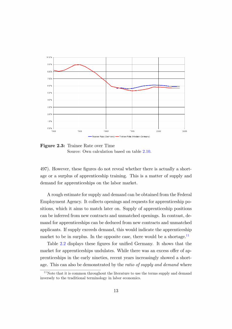
Figure 2.3: Trainee Rate over TimeSource: Own calculation based on table 2.10.

497). However, these �gures do not reveal whether there is actually a short-

age or a surplus of apprenticeship training. This is a matter of supply and

demand for apprenticeships on the labor market.

A rough estimate for supply and demand can be obtained from the Federal

Employment Agency. It collects openings and requests for apprenticeship po-

sitions, which it aims to match later on. Supply of apprenticeship positions

can be inferred from new contracts and unmatched openings. In contrast, de-

mand for apprenticeships can be deduced from new contracts and unmatched

applicants. If supply exceeds demand, this would indicate the apprenticeship

market to be in surplus. In the opposite case, there would be a shortage.11

Table 2.2 displays these �gures for uni�ed Germany. It shows that the

market for apprenticeships undulates. While there was an excess o¤er of ap-

prenticeships in the early nineties, recent years increasingly showed a short-

age. This can also be demonstrated by the ratio of supply and demand where

11Note that it is common throughout the literature to use the terms supply and demandinversely to the traditional terminology in labor economics.

13

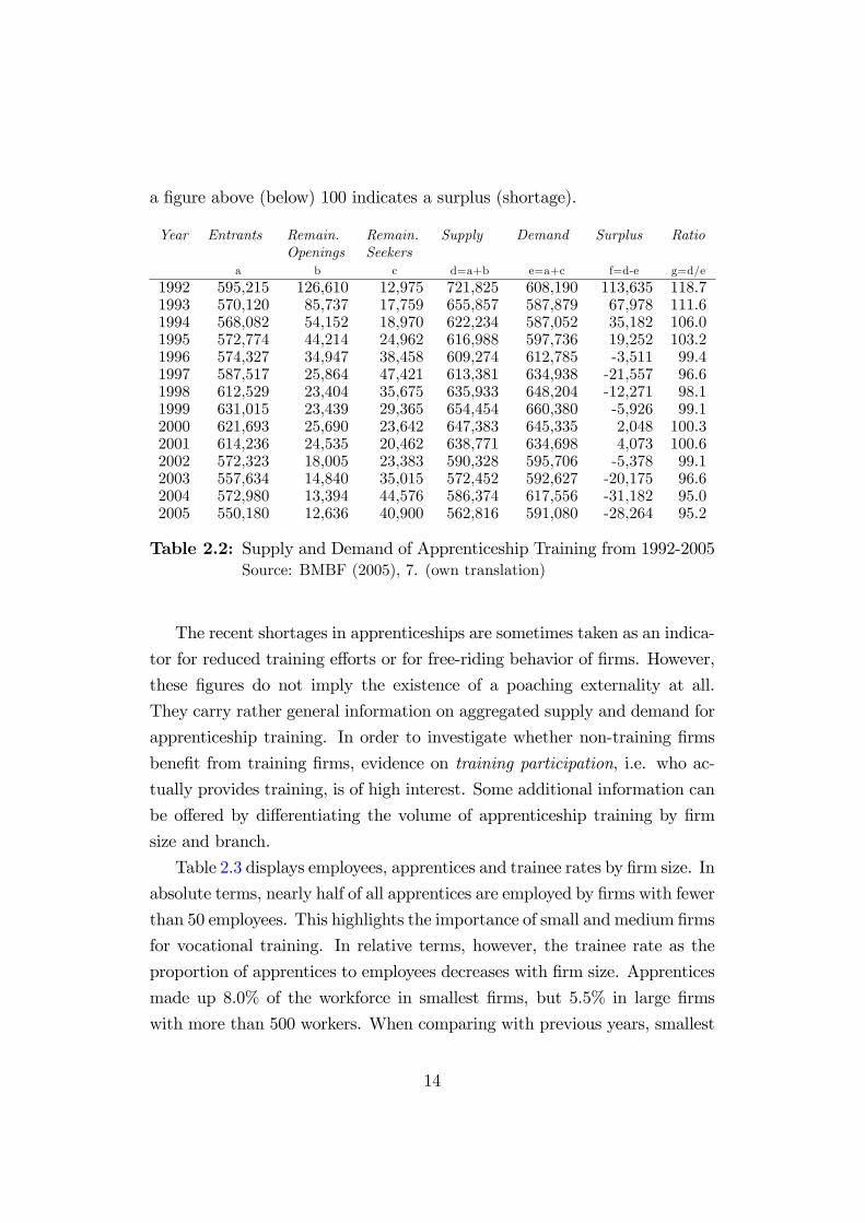
a �gure above (below) 100 indicates a surplus (shortage).

Year Entrants Remain.Openings

Remain.Seekers

Supply Demand Surplus Ratio

a b c d=a+b e=a+c f=d-e g=d/e

1992 595,215 126,610 12,975 721,825 608,190 113,635 118.71993 570,120 85,737 17,759 655,857 587,879 67,978 111.61994 568,082 54,152 18,970 622,234 587,052 35,182 106.01995 572,774 44,214 24,962 616,988 597,736 19,252 103.21996 574,327 34,947 38,458 609,274 612,785 -3,511 99.41997 587,517 25,864 47,421 613,381 634,938 -21,557 96.61998 612,529 23,404 35,675 635,933 648,204 -12,271 98.11999 631,015 23,439 29,365 654,454 660,380 -5,926 99.12000 621,693 25,690 23,642 647,383 645,335 2,048 100.32001 614,236 24,535 20,462 638,771 634,698 4,073 100.62002 572,323 18,005 23,383 590,328 595,706 -5,378 99.12003 557,634 14,840 35,015 572,452 592,627 -20,175 96.62004 572,980 13,394 44,576 586,374 617,556 -31,182 95.02005 550,180 12,636 40,900 562,816 591,080 -28,264 95.2

Table 2.2: Supply and Demand of Apprenticeship Training from 1992-2005Source: BMBF (2005), 7. (own translation)

The recent shortages in apprenticeships are sometimes taken as an indica-

tor for reduced training e¤orts or for free-riding behavior of �rms. However,

these �gures do not imply the existence of a poaching externality at all.

They carry rather general information on aggregated supply and demand for

apprenticeship training. In order to investigate whether non-training �rms

bene�t from training �rms, evidence on training participation, i.e. who ac-

tually provides training, is of high interest. Some additional information can

be o¤ered by di¤erentiating the volume of apprenticeship training by �rm

size and branch.

Table 2.3 displays employees, apprentices and trainee rates by �rm size. In

absolute terms, nearly half of all apprentices are employed by �rms with fewer

than 50 employees. This highlights the importance of small and medium �rms

for vocational training. In relative terms, however, the trainee rate as the

proportion of apprentices to employees decreases with �rm size. Apprentices

made up 8.0% of the workforce in smallest �rms, but 5.5% in large �rms

with more than 500 workers. When comparing with previous years, smallest

14

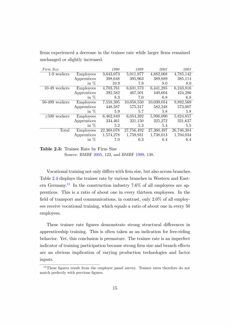
�rms experienced a decrease in the trainee rate while larger �rms remained

unchanged or slightly increased.

Firm Size 1990 1999 2002 20031-9 workers Employees 3,643,073 5,011,977 4,882,068 4,785,142

Apprentices 398,648 395,963 389,889 385,114in % 10.9 7.9 8.0 8.0

10-49 workers Employees 4,703,761 6,631,573 6,441,285 6,243,816Apprentices 392,582 467,501 440,604 424,286

in % 8.3 7.0 6.8 6.850-499 workers Employees 7,558,395 10,058,550 10,039,054 9,892,569

Apprentices 448,587 575,317 582,248 573,007in % 5.9 5.7 5.8 5.8

�500 workers Employees 6,462,849 6,054,392 5,998,090 5,824,857Apprentices 334,461 321,150 325,272 321,627

in % 5.2 5.3 5.4 5.5Total Employees 22,368,078 27,756,492 27,360,497 26,746,384

Apprentices 1,574,278 1,759,931 1,738,013 1,704,034in % 7.0 6.3 6.4 6.4

Table 2.3: Trainee Rate by Firm SizeSource: BMBF 2005, 123, and BMBF 1999, 138.

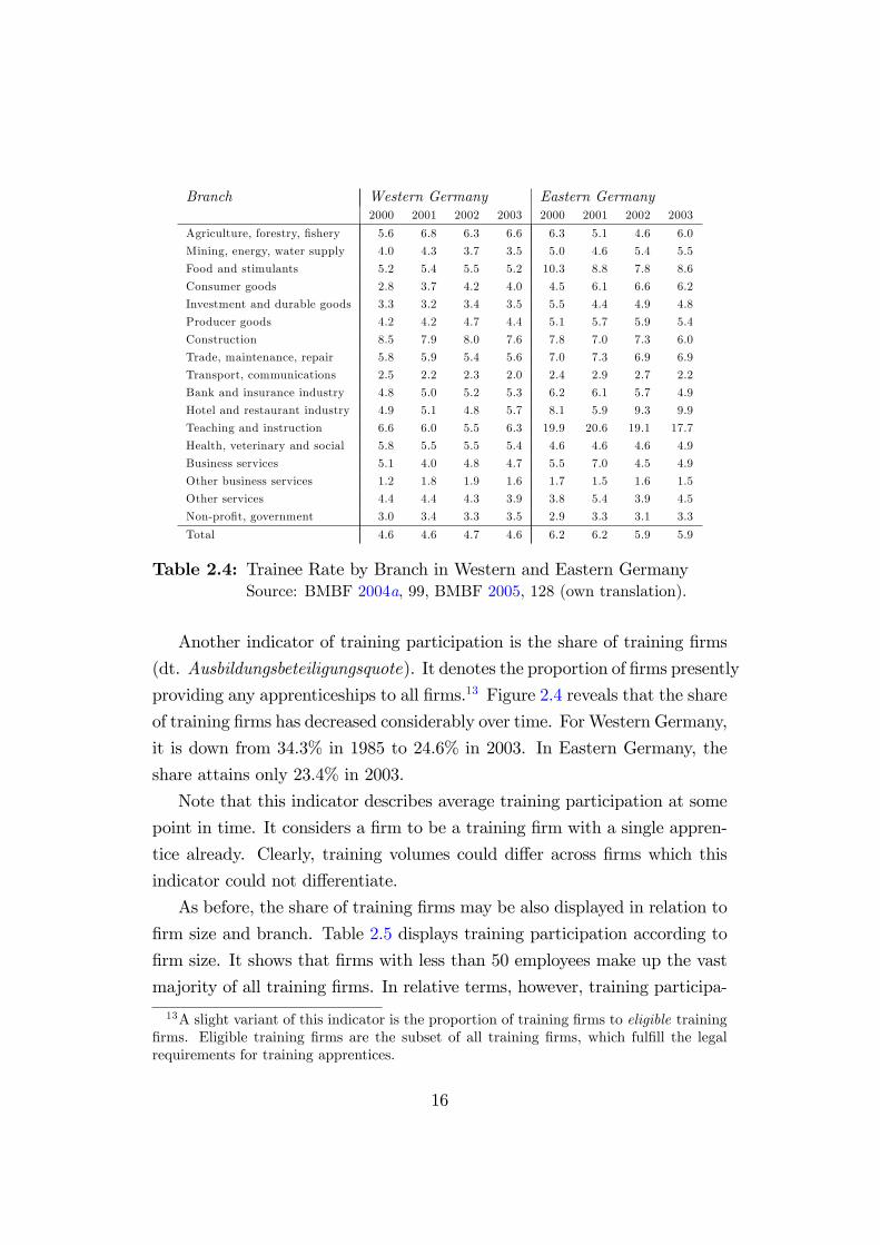
Vocational training not only di¤ers with �rm size, but also across branches.

Table 2.4 displays the trainee rate by various branches in Western and East-

ern Germany.12 In the construction industry 7.6% of all employees are ap-

prentices. This is a ratio of about one in every thirteen employees. In the

�eld of transport and communications, in contrast, only 2.0% of all employ-

ees receive vocational training, which equals a ratio of about one in every 50

employees.

These trainee rate �gures demonstrate strong structural di¤erences in

apprenticeship training. This is often taken as an indication for free-riding

behavior. Yet, this conclusion is premature. The trainee rate is an imperfect

indicator of training participation because strong �rm size and branch e¤ects

are an obvious implication of varying production technologies and factor

inputs.

12These �gures result from the employer panel survey. Trainee rates therefore do notmatch perfectly with previous �gures.

15

Branch Western Germany Eastern Germany2000 2001 2002 2003 2000 2001 2002 2003

Agriculture, forestry, �shery 5.6 6.8 6.3 6.6 6.3 5.1 4.6 6.0

Mining, energy, water supply 4.0 4.3 3.7 3.5 5.0 4.6 5.4 5.5

Food and stimulants 5.2 5.4 5.5 5.2 10.3 8.8 7.8 8.6

Consumer goods 2.8 3.7 4.2 4.0 4.5 6.1 6.6 6.2

Investment and durable goods 3.3 3.2 3.4 3.5 5.5 4.4 4.9 4.8

Producer goods 4.2 4.2 4.7 4.4 5.1 5.7 5.9 5.4

Construction 8.5 7.9 8.0 7.6 7.8 7.0 7.3 6.0

Trade, maintenance, repair 5.8 5.9 5.4 5.6 7.0 7.3 6.9 6.9

Transport, communications 2.5 2.2 2.3 2.0 2.4 2.9 2.7 2.2

Bank and insurance industry 4.8 5.0 5.2 5.3 6.2 6.1 5.7 4.9

Hotel and restaurant industry 4.9 5.1 4.8 5.7 8.1 5.9 9.3 9.9

Teaching and instruction 6.6 6.0 5.5 6.3 19.9 20.6 19.1 17.7

Health, veterinary and social 5.8 5.5 5.5 5.4 4.6 4.6 4.6 4.9

Business services 5.1 4.0 4.8 4.7 5.5 7.0 4.5 4.9

Other business services 1.2 1.8 1.9 1.6 1.7 1.5 1.6 1.5

Other services 4.4 4.4 4.3 3.9 3.8 5.4 3.9 4.5

Non-pro�t, government 3.0 3.4 3.3 3.5 2.9 3.3 3.1 3.3

Total 4.6 4.6 4.7 4.6 6.2 6.2 5.9 5.9

Table 2.4: Trainee Rate by Branch in Western and Eastern GermanySource: BMBF 2004a, 99, BMBF 2005, 128 (own translation).

Another indicator of training participation is the share of training �rms

(dt. Ausbildungsbeteiligungsquote). It denotes the proportion of �rms presently

providing any apprenticeships to all �rms.13 Figure 2.4 reveals that the share

of training �rms has decreased considerably over time. ForWestern Germany,

it is down from 34.3% in 1985 to 24.6% in 2003. In Eastern Germany, the

share attains only 23.4% in 2003.

Note that this indicator describes average training participation at some

point in time. It considers a �rm to be a training �rm with a single appren-

tice already. Clearly, training volumes could di¤er across �rms which this

indicator could not di¤erentiate.

As before, the share of training �rms may be also displayed in relation to

�rm size and branch. Table 2.5 displays training participation according to

�rm size. It shows that �rms with less than 50 employees make up the vast

majority of all training �rms. In relative terms, however, training participa-

13A slight variant of this indicator is the proportion of training �rms to eligible training�rms. Eligible training �rms are the subset of all training �rms, which ful�ll the legalrequirements for training apprentices.

16

Figure 2.4: Share of Training FirmsSource: Own calculation based on table 2.10.

tion increases with �rm size. Only 16.8% of smallest �rms train, while this

share attains 90.4% for large �rms.14

Clearly, training participation also di¤ers across branches. Table 2.6 de-

picts the share of training �rms by branch separate for Western and Eastern

Germany. A high training participation can be observed in food, investment

goods, construction, or health, while transport or business services show

rather low participation rates.

Despite their shortcomings, the �gures to this point indicate vocational

training to be declining. As some demand for vocational training remains

unmatched, shortages of apprenticeships are present. However, even though

training participation by �rms is small and declining, this does not imply an

externality problem. Above �gures rather imply structural changes in the

demand and supply for apprenticeships.

In order to substantiate the claim of positive training spillovers, which

could principally account for some training shortages, more knowledge is

14Firms�training participation according to �rm size is sometimes referred to as densityof training �rms (dt. Ausbildungsbetriebsdichte).

17

Firm Size 1990 1999 2002 20031-9 workers All �rms 1,237,052 1,708,241 1,670,382 1,644,449

Training �rms 264,984 282,915 277,090 275,542in % 21.4 16.6 16.6 16.8

10-49 workers All �rms 236,762 333,384 323,120 312,842Training �rms 122,439 157,879 148,051 143,939

in % 51.7 47.4 45.8 46.050-499 workers All �rms 59,063 81,168 80,679 79,542

Training �rms 43,494 55,929 54,322 54,249in % 73.6 68.9 67.3 68.2

�500 workers All �rms 4,794 5,038 4,976 4,829Training �rms 4,508 4,603 4,496 4,366

in % 94.0 91.4 90.4 90.4Total All �rms 1,537,671 2,127,831 2,079,157 2,041,662

Training �rms 435,425 501,326 483,959 478,096in % 28.3 23.6 23.3 23.4

Table 2.5: Share of Training Firms by Firm SizeSource: BMBF (1999), 137, BMBF (2005), 122.

Branch Western Germany Eastern Germany2000 2001 2002 2003 2000 2001 2002 2003




Consumer goods 22.2 40.0 38.5 34.8 28.1 41.6 39.3 40.1


Producer goods 43.7 39.0 44.3 40.0 39.9 45.9 44.2 45.1

Construction 47.0 44.4 45.8 40.8 35.9 34.3 34.3 29.5









Other services 27.6 29.3 29.4 25.7 21.9 23.2 17.1 19.2


Total 29.7 30.4 31.3 29.9 26.1 27.0 25.7 25.0

Table 2.6: Share of Training Firms by Branch in Western and Eastern Ger-manySource: BMBF (2005), Table 49, 123 (own translation).

18

needed. In particular, we require information on whether training is costly

to �rms and whether non-training �rms bene�t from this e¤ort. We will

therefore now have a closer look at the �nancing of training.

2.2.2 Financing Training

Firms that employ apprentices for vocational training incur costs. These

costs consist of direct costs and also indirect costs. Expenses for training

materials and trainee wages are examples for the former category whereas

foregone production of experienced workers are examples for the latter. At

the same time, �rms also receive bene�ts from training. Similar to costs,

these can be direct bene�ts and indirect bene�ts. The productive output of

apprentices denotes an example for direct bene�ts. In contrast, savings on

future recruitment costs are of an indirect nature since they arise only if

apprentices enter into a regular employment after training.

Several studies seek to estimate the net position of �rms from appren-

ticeship training. Bardeleben et al. (1995) use an accounting approach in

order to estimate the yearly training costs per apprentice. They conduct an

employer survey for information on four cost categories: personnel costs of

apprentices, personnel costs of instructors, equipment costs, and other costs.

Figure 2.5 displays their classi�cation of training costs.

Figure 2.5: Gross Costs of Apprenticeship TrainingSource: Shorted translation of Bardeleben et al. (1995), 27.

19

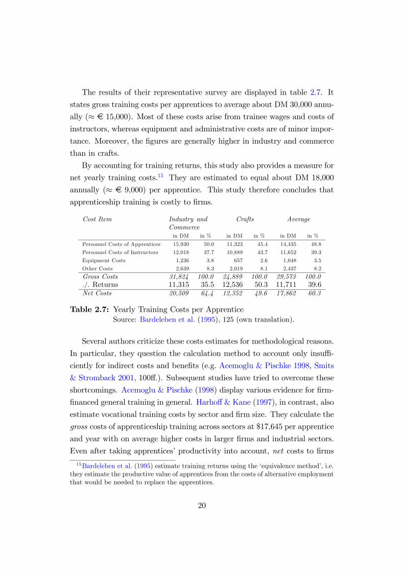
The results of their representative survey are displayed in table 2.7. It

states gross training costs per apprentices to average about DM 30,000 annu-

ally (� e 15,000). Most of these costs arise from trainee wages and costs of

instructors, whereas equipment and administrative costs are of minor impor-

tance. Moreover, the �gures are generally higher in industry and commerce

than in crafts.

By accounting for training returns, this study also provides a measure for

net yearly training costs.15 They are estimated to equal about DM 18,000

annually (� e 9,000) per apprentice. This study therefore concludes that

apprenticeship training is costly to �rms.

Cost Item Industry andCommerce

Crafts Average

in DM in % in DM in % in DM in %

Personnel Costs of Apprentices 15,930 50.0 11,323 45.4 14,435 48.8

Personnel Costs of Instructors 12,018 37.7 10,889 43.7 11,652 39.3

Equipment Costs 1,236 3.8 657 2.6 1,048 3.5

Other Costs 2,639 8.3 2,019 8.1 2,437 8.2

Gross Costs 31,824 100.0 24,889 100.0 29,573 100.0./. Returns 11,315 35.5 12,536 50.3 11,711 39.6Net Costs 20,509 64.4 12,352 49.6 17,862 60.3

Table 2.7: Yearly Training Costs per ApprenticeSource: Bardeleben et al. (1995), 125 (own translation).

Several authors criticize these costs estimates for methodological reasons.

In particular, they question the calculation method to account only insu¢ -

ciently for indirect costs and bene�ts (e.g. Acemoglu & Pischke 1998, Smits

& Stromback 2001, 100¤.). Subsequent studies have tried to overcome these

shortcomings. Acemoglu & Pischke (1998) display various evidence for �rm-

�nanced general training in general. Harho¤& Kane (1997), in contrast, also

estimate vocational training costs by sector and �rm size. They calculate the

gross costs of apprenticeship training across sectors at $17,645 per apprentice

and year with on average higher costs in larger �rms and industrial sectors.

Even after taking apprentices�productivity into account, net costs to �rms

15Bardeleben et al. (1995) estimate training returns using the �equivalence method�, i.e.they estimate the productive value of apprentices from the costs of alternative employmentthat would be needed to replace the apprentices.

20

remain high at $10,657 per apprentice and year, or 60% of the gross costs.

2.2.3 Turnover and Poaching

The last section provided some evidence that vocational training is on average

costly to �rms. If �rms are pro�t-seeking, then this implies an apprentice-

ship to be an investment in expectation of future returns. Otherwise, these

expenses could be allocated in alternative uses. However, if trained workers

are poached by competitors, this investment could be lost and give rise to

positive spillovers.

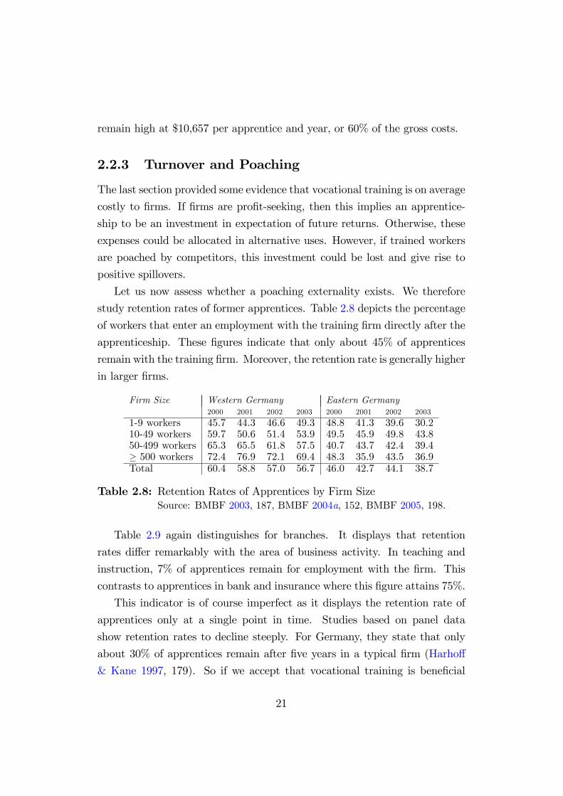
Let us now assess whether a poaching externality exists. We therefore

study retention rates of former apprentices. Table 2.8 depicts the percentage

of workers that enter an employment with the training �rm directly after the

apprenticeship. These �gures indicate that only about 45% of apprentices

remain with the training �rm. Moreover, the retention rate is generally higher

in larger �rms.

Firm Size Western Germany Eastern Germany2000 2001 2002 2003 2000 2001 2002 2003

1-9 workers 45.7 44.3 46.6 49.3 48.8 41.3 39.6 30.210-49 workers 59.7 50.6 51.4 53.9 49.5 45.9 49.8 43.850-499 workers 65.3 65.5 61.8 57.5 40.7 43.7 42.4 39.4� 500 workers 72.4 76.9 72.1 69.4 48.3 35.9 43.5 36.9Total 60.4 58.8 57.0 56.7 46.0 42.7 44.1 38.7

Table 2.8: Retention Rates of Apprentices by Firm SizeSource: BMBF 2003, 187, BMBF 2004a, 152, BMBF 2005, 198.

Table 2.9 again distinguishes for branches. It displays that retention

rates di¤er remarkably with the area of business activity. In teaching and

instruction, 7% of apprentices remain for employment with the �rm. This

contrasts to apprentices in bank and insurance where this �gure attains 75%.

This indicator is of course imperfect as it displays the retention rate of

apprentices only at a single point in time. Studies based on panel data

show retention rates to decline steeply. For Germany, they state that only

about 30% of apprentices remain after �ve years in a typical �rm (Harho¤

& Kane 1997, 179). So if we accept that vocational training is bene�cial

21

Sector Western Germany Eastern Germany2000 2001 2002 2003 2000 2001 2002 2003




Consumer goods 65.3 55.0 60.9 55.0 74.5 67.0 51.8 49.6


Producer goods 70.8 84.9 80.0 79.0 74.3 72.4 69.6 65.1

Construction 63.0 64.7 56.3 54.2 50.3 48.1 48.9 44.2









Other services 52.6 42.4 52.9 56.3 75.3 32.4 62.0 51.4


Total 60.4 58.8 57.0 56.7 46.0 42.7 44.1 38.7

Table 2.9: Retention Rates of Apprentices by BranchSource: BMBF 2002, 487, BMBF 2003, 187, BMBF 2004a, 153,BMBF 2005, 199 (own translation).

for several consecutive periods, this strongly supports the claim of positive

training spillovers.

2.3 Discussion

This chapter provided a short introduction to the German apprenticeship

system. It pointed out that rules and institutions strongly formalize and

regulate apprenticeship training. This is to ensure that apprenticeships o¤er

quite general skills that are widely applicable within a profession. A voca-

tional degree can thus be regarded as a standard vocational quali�cation that

is commonly accepted across �rms.

A rough survey of statistics and empirical studies then sought to under-

stand who actually provides and �nances apprenticeship training and whether

there is evidence for a poaching externality. The absolute count of appren-

tices underlined the importance of the apprenticeship system for vocational

22

education in Germany. Yet, several indicators pointed to the fact that the

volume of training as well as the participation by �rms have declined in re-

cent years. While this could result from structural changes, it could also be

shown that training �rms bear an important share of the training costs and

face a considerable risk of apprentices quitting after training. Although these

�gures di¤er strongly with �rm size and sector, they are supportive to the

claim of apprenticeship training giving rise to training spillovers. Thus, in

light of these stylized facts, there is a need to theoretically investigate whether

poaching induces training spillovers and whether training policy could have

a mitigating role.

23

2.A Appendix

Year Employees Apprentices Entrants Trainee RateWestern Germany

1980 20,953,864 1,715,481 669,901 8.19%1985 20,378,397 1,831,501 709,322 8.99%1990 22,368,078 1,476,880 538,179 6.60%1991 23,409,885 1,391,010 515,667 5.94%1995 22,547,730 1,194,043 434,934 5.30%2000 22,323,721 1,297,202 482,913 5.81%2001 22,356,509 1,296,327 474,761 5.80%2002 22,036,653 1,255,634 441,898 5.70%2003 21,555,574 1,226,492 436,873 5.69%2004 21,342,537 1,214,024 445,559 5.69%

Uni�ed Germany

1991 30,000,000 1,665,618 613,852 5.55%1995 28,057,050 1,579,339 578,582 5.63%2000 27,979,593 1,702,017 622,967 6.08%2001 27,864,091 1,684,669 609,576 6.05%2002 27,360,497 1,622,441 568,082 5.93%2003 26,746,384 1,581,629 564,493 5.91%2004 26,381,842 1,564,064 571,978 5.93%

Table 2.10: Volume of Employees, Apprentices, and EntrantsSource: StBA 2005a, 12, 24, 42; StBA 2005b, 76.

24

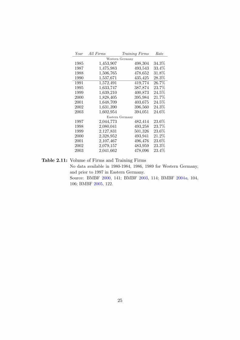
Year All Firms Training Firms RateWestern Germany

1985 1,453,907 498,304 34.3%1987 1,475,983 493,543 33.4%1988 1,506,765 478,652 31.8%1990 1,537,671 435,425 28.3%1991 1,572,491 419,774 26.7%1995 1,633,747 387,874 23.7%1999 1,639,210 400,873 24.5%2000 1,828,405 395,984 21.7%2001 1,648,709 403,675 24.5%2002 1,631,390 396,560 24.3%2003 1,602,954 394,051 24.6%

Eastern Germany

1997 2,044,773 482,414 23.6%1998 2,080,041 493,258 23.7%1999 2,127,831 501,326 23.6%2000 2,328,952 493,941 21.2%2001 2,107,467 496,476 23.6%2002 2,079,157 483,959 23.3%2003 2,041,662 478,096 23.4%

Table 2.11: Volume of Firms and Training FirmsNo data available in 1980-1984, 1986, 1989 for Western Germany,and prior to 1997 in Eastern Germany.Source: BMBF 2000, 141; BMBF 2003, 114; BMBF 2004a, 104,106; BMBF 2005, 122.

25

Chapter 3

Vocational Training andPositive Spillovers

The question of positive spillovers from vocational training has long ago at-

tracted the interest of economists. Early contributions hinted at the problem

of positive externalities accruing to society and proposed policy measures to

improve welfare. Later contributions, quite to the contrary, questioned the

existence of such positive spillovers and o¤ered completely di¤erent policy

conclusions. In light of these opposing views, a short review of the literature

on vocational education and positive spillovers seems strongly mandated.1

3.1 Theoretic Precursors

The existence of educational spillovers has already been claimed by classical

economists. Smith (1776), in his renowned contribution, emphasizes that

education positively a¤ects social life beyond mere skill acquisition. In view

of these social bene�ts he derives a role for the state in providing basic

education and suggests partial public contributions.

�For a very small expen[s]e the public can facilitate, can en-

courage, and can even impose upon almost the whole body of

1For an extended overview on the history of educational economics see, for instance,Pfahler (2000).

26

the people, the necessity of acquiring [the] most essential parts

of education. The public can facilitate this acquisition by estab-

lishing in every parish or district a little school [...]; the master

being partly, but not wholly, paid by the public, because, if he

was wholly, or even principally, paid by it, he would soon learn

to neglect his business.�(Smith 1776, 990)

While Smith�s analysis was concerned with education in general and with

incentives for instructors in particular, later writers dealt more speci�cally

with industrial training. Marshall (1920) compared basic education to a

technical education for a particular occupation. He also distinguished general

abilities from specialized abilities, with the former applicable in all industries

and the latter only in an individual trade. Moreover, he pointed out that

public and private expenditures into training should not be measured on the

basis of their direct returns alone (Marshall 1920, IV, Ch. vi, §3.).

Simultaneous with the industrial revolution, economists increasingly ob-

served a lack of technical education. On the one hand, universal apprentice-

ship training declined as machines and assembly lines replaced manual tech-

niques and pushed traditional trades and crafts aside. On the other hand, the

expanding industrial sector o¤ered only little on-the-job training. Industrial

workers were left to execute simple and repeatable tasks, despite striking

opportunities to enlarge their skills and quali�cations Smits & Stromback

(2001).

This development led to concerns on whether technical education was an

employer obligation or foremost a public duty. Pigou (1912) is acknowledged

for the �rst economic analysis of on-the-job training. He emphasized that a

training �rm may be inhibited from obtaining the full returns to its train-

ing e¤orts because, with some workers quitting for another �rm, the new

employer also participates in the returns to training. Thereby he identi�ed

poaching as the source of the discrepancy between private and social returns

to training. The following quotation illustrates this idea.

�It is, however, obvious that openings exist for investments

by the tenant (i.e. the employer) in workpeople�s capacity, which

27

would yield considerable social net product. Under a slave econ-

omy, since the employer could secure for himself the whole result

of increased e¢ ciency in his workpeople and their families, the

whole of the social net product of any unit of resources invested in

the improvement of their quality would be represented in private

net product. Under a free economy, however, since workpeople

are liable to change employers, and so to deprive investing ten-

ants of the fruits of their investment, the private net product is

apt to fall considerably short of the social net product. Hence, so-

cially pro�table expenditure by employers in the training of their

workpeople, in building up their health, and in defending them

against accident does not carry a corresponding private pro�t.�

(Pigou 1912, 153)

Pigou observed that this positive spillover from training is lost to the

investing �rm, but not to society as a whole. From a social point of view,

therefore, training will be undersupplied because private investment is only

carried out up to the point where additional private returns equal the ad-

ditional costs. With the extra social returns not taken into account by the

training �rm, welfare falls short of its optimal level.

Following this assessment of the economic situation, Pigou identi�ed a

possible role for the state to improve overall welfare. He proposed to intro-

duce �scal incentives to private activities that bring about additional returns

to society and, vice versa, �scal disincentives to private activities that entail

social costs. With such a policy, the social externalities caused by an action

can be attributed to an individual decision and will thereby lead to a true

economic calculation. Modern economists now commonly refer to this policy

instrument as �Pigouvian subsidy�or �Pigouvian tax�.

�It is plain that divergences between private and social net

product of the kind just considered cannot [...] be mitigated by

a modi�cation of the contractual relation between any two con-

tracting parties, because the divergence arises out of a service or

disservice rendered to persons other than the contracting parties.

28

It is, however, possible for the State, if it so chooses, to remove

the divergence in any �eld by �extraordinary encouragements�or

�extraordinary restraints� upon investments in that �eld. The

most obvious forms, which these encouragements and restraints

may assume, are, of course, those of bounties and taxes.�(Pigou

1912, 164)

While a Pigouvian tax deliberately discourages the taxed activity and

brings about some revenues, a Pigouvian subsidy, by contrast, requires addi-

tional �nancial resources in order to encourage socially bene�cial activities.

Public funds are however scarce. Thus, in case subsidies are introduced, ei-

ther alternative public spending is to be discarded or additional funds must

be collected. Pigou noted that raising tax revenue in�icts costs on society.

Therefore, in case subsidies are introduced to encourage activities bene�cial

to social welfare, their bene�ts are to exceed their �nancial costs.

�The raising of an additional £ of revenue ... in�icts indirect

damage on the taxpayers as a body over and above the loss they

su¤er in actual money payment. Where there is indirect damage,

it ought to be added to the direct loss of satisfaction involved

in the withdrawal of the marginal unit of resources by taxation,

before this is balanced against the satisfaction yielded by the

marginal expenditure.�(Pigou 1947, 33-34)

Economists widely accepted Pigou�s conjecture of a poaching externality

in vocational education. In light of his theoretical assessment, public policy

supported a stronger public role in vocational education. Several countries

introduced �scal incentives towards vocational training, both in the form

of training grants and training levies. See below in section 5.3.1 for some

examples.

However, Pigou�s assessment of training, as well as the role of public

policy therein, became challenged by human capital theory. It led to major

revisions in the economics of on-the-job training.

29

3.2 On-the-JobTraining inPerfect LaborMarkets

In contrast to neoclassical economics, human capital theory endorsed a more

general concept of capital that allowed in particular for human resources.

In analogy to physical or �nancial capital, human capital is perceived as

the stock of knowledge, skills, health, or abilities that is embodied in a per-

son and that can be put to productive work. Moreover, human capital can

be increased, alike investments in physical or �nancial capital, by training,

schooling or health provisions (Becker 1962, 11).2

Despite its intuitive economic appeal, the concept of human capital has

been the subject of severe debates. In particular, there is a great reluctance

to model people as a stock of capital, worrying to reduce mankind to a

mere material category. Only recently, the term �human capital�received the

yearly doublespeak award for particularly obscure terminology by a German

language watch association Schlosser (2005).

Although understandable from an ethical point of view, this concern can

clearly be refuted. Rather than belittling the human nature, human capital

theory recognizes the importance of people for economic growth and social

progress. Irrespective of its unaesthetic semantics and inherent conceptual

limitations, it incorporates the value of education, training, health, and social

relationships into economic theory. Moreover, the notion of a capital stock

of human resources embodies positive economic properties. Once skills and

knowledge have been invested and built up, they enable people to reap a

steady �ow of economic returns. Thereby their choices and welfare increase

(Schultz 1961, 2).

In a well-known contribution, Becker (1962) analyzes incentives for hu-

man capital investments. He focuses in particular on motives for on-the-

2Initially, the human capital literature drew attention to the shortcomings of neoclassi-cal economics and criticized in particular the prevailing assumption of homogeneous labor.It pointed out that the growth in per capita incomes across countries cannot be explainedby using a standard production function approach with stocks of land and capital andthe size of the workforce. Therefore, early propopents of human capital theory (Schultz1961, Becker 1962, Mincer 1974, e.g.) urged to reconsider the representation of people ineconomic models. They emphasized to account for workers�skills and knowledge as keydeterminants of economic performance.

30

job training and questions the emergence of positive spillovers. In contrast

to school training, on-the-job training is carried out at the workplace and

through the �rm. It raises the productivity of the workforce in the future,

but it involves costs to the training �rm at present, such as time, e¤ort, ma-

terial, and equipment. Becker points out that resources spent for on-the-job

training compete with alternative investment opportunities. Consequently,

a �rm that incurs additional costs or lower revenues from providing training

at present necessarily expects larger revenues or fewer expenditures in the

future.

Since Becker�s assessment of on-the-job training possesses a central place

in the training literature, let us sketch his approach. Let Et and Rt denote

expenditures and receipts from on-the-job training by a �rm in period t.

Moreover, let r be the market rate of interest. Analogous to investments in

physical or �nancial assets, an investment in human capital is carried out

at most so that the present value of expenditures equals those of receipts.

Thus, a �rm carries out a human capital investment to the extent of ful�lling

equation (3.1).nXt=0

Rt(1 + r)t

=nXt=0

Et(1 + r)t

(3.1)

The receipts of on-the-job training are the increased marginal product of the

worker, while expenditures obviously consist of training costs and wages to

employ the worker.

Assume further that training be only given during the initial period, t = 0.

With vt referring to the worker�s marginal product in period t, wt being the

wage paid to the worker and k standing for any training expenses, the �rms

investment condition can be rewritten to

v0 +nXt=1

vt(1 + r)t

= w0 + k +nXt=1

wt(1 + r)t

(3.2)

Becker de�nes G as the excess of future receipts over future outlays, i.e.

G =Pn�1

t=1vt�wt(1+r)t

. It can be interpreted as a measure of the return of on-the-

31

job training to the �rm. Using G, equation (3.2) simpli�es to

v0 +G = w0 + k (3.3)

This states that trainings costs and wage payments in the training period

are equal to the marginal productivity and the return from training.

Note that k only measures actual training expenses, but excludes oppor-

tunity costs from training. Clearly, if the worker were not receiving training,

she could produce vu0 instead of v0, where vu0 denotes the marginal product

of an unskilled worker. Total training costs c thus are the sum of actual

expenses and opportunity costs, c = (vu0 � v0) + k. Inserting into condition

(3.3) then obtains

vu0 +G = w0 + c (3.4)

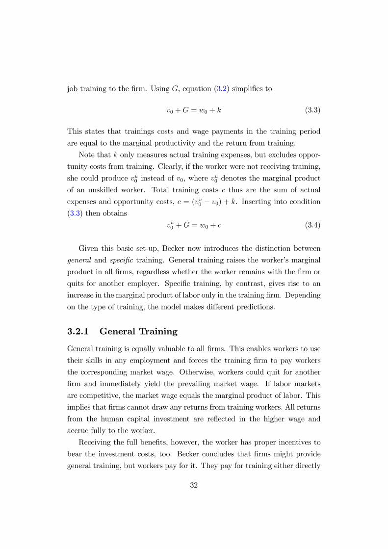
Given this basic set-up, Becker now introduces the distinction between

general and speci�c training. General training raises the worker�s marginal

product in all �rms, regardless whether the worker remains with the �rm or

quits for another employer. Speci�c training, by contrast, gives rise to an

increase in the marginal product of labor only in the training �rm. Depending

on the type of training, the model makes di¤erent predictions.

3.2.1 General Training

General training is equally valuable to all �rms. This enables workers to use

their skills in any employment and forces the training �rm to pay workers

the corresponding market wage. Otherwise, workers could quit for another

�rm and immediately yield the prevailing market wage. If labor markets

are competitive, the market wage equals the marginal product of labor. This

implies that �rms cannot draw any returns from training workers. All returns

from the human capital investment are re�ected in the higher wage and

accrue fully to the worker.

Receiving the full bene�ts, however, the worker has proper incentives to

bear the investment costs, too. Becker concludes that �rms might provide

general training, but workers pay for it. They pay for training either directly

32

or indirectly via wage reductions in the investment period. Moreover, as all

returns accrue to the worker, there are no spillovers from general training on

other �rms. Thus, contrary to Pigou, training is e¢ cient (Becker 1962, 17).

Formally, if training is general and labor markets are competitive, wages

are equal to worker�s marginal product, wt = vt. As G = 0, there are conse-

quently no returns from on-the-job training to the �rm. From the investment

condition then follows equation (3.5)

w0 = v0 � k = vu0 � c (3.5)

This clearly shows that the wage in the training period is reduced by the

training costs, which implies that all costs of general training are incurred

by the worker.

3.2.2 Speci�c Training

For speci�c training, Becker argues that �rms will be able to recover training

costs. The worker cannot gain from quitting as these skills are of no use

to other �rms. Thus, the competitive market wage remains una¤ected and

the training �rm captures all returns from speci�c training in the form of

increased worker productivity.

Formally, if training returns are speci�c, we now have G > 0. Firm

optimal training investment is equal to G = c, and the investment condition

then simpli�es to

w0 = vu0 (3.6)

This states in contrast to general training that worker�s training wage remains

una¤ected if training is speci�c. But since this investment is rewarding only

as long as the worker stays with the �rm, some of the returns from this

investment will be shared between the �rm and the worker in order to prevent

workers from quitting. Also note that all returns are again collected by the

private parties. Hence, there are no spillovers on other �rms by this type of

investment and speci�c training is e¢ cient (Becker 1962, 21).

33

In sum, standard human capital theory negates positive spillovers from

vocational training. As private and social returns do not diverge, human capi-

tal investment will be at its socially optimal level. General training is paid for

by the worker, speci�c training by both the employer and the worker. Becker

acknowledges that insu¢ cient general training may indeed arise if workers

are exposed to credit constraints and/or are risk averse (Becker 1962, 41f.).

In this case, however, training subsidies or public training provision are not

warranted. Rather, educational policy should address the problems prevail-

ing in credit and insurance markets that cause these training limitations.

Although standard human capital theory is theoretically appealing, it

faces profound criticism. Firstly, it is (at least partially) contradicted by

empirical evidence. In contrast to its central proposition, a large number of

empirical studies con�rm the existence of �rm-provided and �rm-�nanced

general training. Despite the risk of quits, �rms actually incur substantial

training costs to provide their workforce with general skills. This has also

been demonstrated for apprenticeship training.3

Secondly, human capital theory is unable to explain some common fea-

tures of apprenticeship training, such as the �xed duration of training con-

tracts or the restrictions on unilateral termination. Under the assumption

of competitive labor markets with full information and perfect contracting,

these particularities should be super�uous (Smits & Stromback 2001, 32).

3.3 On-the-JobTraining in Imperfect LaborMarkets

The contradictions between human capital theory and empirical evidence

have ignited new interest in the economics of training. Modern research

seeks to o¤er rationales for �rm-�nanced general training. In particular, it

analyzes on-the-job training in the context of imperfect competition. Even

though Becker already noted the role of labor market conditions, he left

oligopsonistic labor markets unconsidered and regarded the dichotomy of

general and speci�c skills a useful simpli�cation.

3See supra in section 2.2.2.

34

3.3.1 Wage Compression

Several recent contributions question the assumption of a perfect labor mar-

ket for general skills altogether and analyze training technology and labor

market conditions separately. In order to explain �rm-�nanced general train-

ing these studies commonly feature labor market imperfections that give rise

to a compressed wage structure. In such a setting, �rms can extract a rent

from employing skilled workers, as the market wage is below the marginal

product of labor.

The reasoning is as follows: General training increases the marginal prod-

uct of labor. Because of the compressed wage structure, however, wages in-

crease to a smaller degree. This turns technologically general skills into de

facto �rm-speci�c skills. Contrary to standard human capital theory it is

therefore pro�table for a �rm to �nance general training. In the optimum, a

�rm will provide a training level where the marginal increase in the rent is

equal to the marginal cost of training.

Acemoglu & Pischke (1998) o¤er a simple formal set-up. Let v(x) describe

a worker�s marginal product resulting from �rm�s training e¤orts x. With

training possessing positive and diminishing marginal returns, the function is

increasing and concave, v0 > 0, v00 < 0. Denote training costs by c(x). They

are commonly assumed to increase convex in the amount of training, c0 > 0,

c00 < 0. Moreover, denote the market wage by w (x). Thus, rational �rms will

choose x such as to maximize the pro�t function � = v (x)� w (x)� c (x).

In competitive labor markets, wages correspond to the marginal product

of labor, v (x) = w (x) and �rms do not carry any training costs. Workers

however are willing to invest in training such that w0 (x�) = v0 (x�) = c0 (x�).

In order for �rms to provide training, workers must incur a wage cut 4. Thisis Becker�s result, which is displayed in �gure (3.1).

This contrasts with the situation of imperfect competition. If labor mar-

ket frictions compress the wage structure, then the market wage w(x) does

not increase to v(x), but only to a lesser degree. This inhibits workers from

obtaining a wage corresponding to their marginal product and allows the �rm

to earn a rent from employment 4(x). A rational �rm will carry out train-

35

Figure 3.1: General Training in Competitive Labor MarketsSource: Acemoglu & Pischke (1999), F118.

ing such that the marginal increase in the rent corresponds to the marginal

training costs, 40 �xf� = c0�xf�. See �gure (3.2).

This set-up predicts �rms to �nance some general training even though

workers are mobile and able to quit. But will human capital investment

also be carried out to a socially optimal extent? In these models training

is necessarily accompanied by a positive externality. Labor market frictions

cause workers not to react instantaneously to wage di¤erentials. They yield

rents to �rms and thereby provide training incentives. While frictions re-

duce turnover, they cannot inhibit quits entirely. Thus, positive spillovers

arise because non-training �rms bene�t from training by employing workers

trained in other �rms without requiring a wage payment equal to the mar-

ginal product of labor. This is commonly referred to as poaching.4 With an

externality present, private incentives are insu¢ cient and training will not

4More precisely, poaching may be active or passive in nature, i.e. attempts to recruitskilled workers may be systematic or resulting from general job turnover. However, we donot pursuit this distinction further.

36

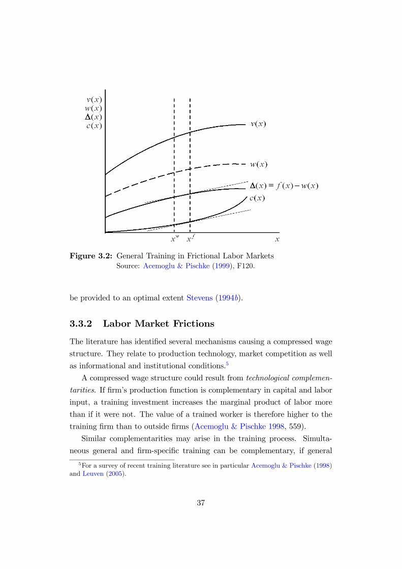
Figure 3.2: General Training in Frictional Labor MarketsSource: Acemoglu & Pischke (1999), F120.

be provided to an optimal extent Stevens (1994b).

3.3.2 Labor Market Frictions

The literature has identi�ed several mechanisms causing a compressed wage

structure. They relate to production technology, market competition as well

as informational and institutional conditions.5

A compressed wage structure could result from technological complemen-

tarities. If �rm�s production function is complementary in capital and labor

input, a training investment increases the marginal product of labor more

than if it were not. The value of a trained worker is therefore higher to the

training �rm than to outside �rms (Acemoglu & Pischke 1998, 559).

Similar complementarities may arise in the training process. Simulta-

neous general and �rm-speci�c training can be complementary, if general

5For a survey of recent training literature see in particular Acemoglu & Pischke (1998)and Leuven (2005).

37

skills are a prerequisite to speci�c skills, or both training types use the same

training infrastructure (Franz & Soskice 1995, 219f.).

Competitive conditions on the output market could also account for wage

compression. Hentschirsch (1999) analyzes training investments for product

markets that are characterized by Cournot or Bertrand competition. Simi-

larly, Gersbach & Schmutzler (2003) show in a game-theoretic structure that

�rms will provide training when competition on the �nal market is su¢ ciently

soft.

Another source of wage compression may be informational asymmetries.

In a pioneering contribution, Katz & Ziderman (1990) show that when train-

ing is not veri�able to outside �rms, workers will be unable to receive a wage

re�ecting their training level. In comparison to other �rms, the training �rm

has an informational advantage with respect to both training quantity or

quality. Consequently, training will be worthwhile, as productivity increases

more than wage payments.

In a similar manner, a training �rm could possess superior knowledge

about a worker�s characteristics, i.e. worker�s innate abilities, talents and

personal qualities. These characteristics are however di¢ cult to assess by

other �rms because they do not draw on work experience. Facing asymmet-

ric information, these employers will only pay for average abilities whereby

outside wage o¤ers could fall short of a worker�s marginal product (Acemoglu

& Pischke 1998, 556f.).

Other labor market frictions impeding workers to quit instantaneously

for outside �rms may result from mobility restrictions. Job turnover is costly

to workers due to search costs, search uncertainties and matching problems.

Workers will abstain from perfect job turnover in regard of the costs associ-

ated with it. Again, the employing �rm can appropriate a rent and wages

are compressed, rendering general training investments pro�table Holzner

(2005).

Finally, labor market institutions have been identi�ed to cause wage com-

38

pression, e.g., through minimum wages, collective bargaining, dismissal pro-

tection and unions Acemoglu & Pischke (1998), Smits & Stromback (2001).

3.4 Discussion

In sum, labor market imperfections allow for an explanation of �rm-�nanced

vocational training. But they also assert the existence of a positive exter-

nality. This contrasts with conventional human capital theory and there-

fore invites to reconsider appropriate public policy. However, comprehensive

studies analyzing di¤erent policy instruments are lacking. The next chapter

therefore introduces a simple model in order to put di¤erent policy instru-

ments into analysis.

39

Chapter 4

Simple Model of VocationalTraining

This chapter proposes a simple model of apprenticeship training. By con-

sidering an oligopsonistic labor market with frictions, the model allows to

explain why �rms partially �nance vocational training. At the same time,

an externality can be shown to exist which leads to insu¢ cient training. In

the appendix and in later chapters, the limiting assumptions of this model

will be relaxed and further complications will be added.

4.1 Model Set-up and Assumptions

Consider an economy where �rms rely on skilled workers to produce goods

and services. Firms can obtain skilled workers in two ways: On the one hand,

they can train unskilled workers by o¤ering apprenticeship training. On the

other hand, they can recruit skilled workers through the labor market by

o¤ering competitive wages.

Wage Competition for Skilled LaborLet �rms compete for the services of skilled workers by posting wage o¤ers.

Workers arbitrage between �rms�wage o¤ers and choose to work for the

�rm with the highest wage. If labor markets were perfect, workers would

40

instantaneously move to the highest paying �rm. This forces �rms to pay

skilled workers a wage equal to their marginal product. In such a situation

�rms cannot obtain any return for general training expenses. They would

therefore shift the costs of training onto trained workers or provide no general

training at all. Essentially, this is the standard result of human capital theory

according to Becker (1962).

In reality, labor markets are imperfect. Skilled individuals usually do not

quit a �rm instantaneously, although they could obtain a somewhat higher

wage elsewhere. The literature review above in section 3.3 has speci�ed a

number of labor market frictions that inhibit workers from perfect wage ar-

bitrage, such as search and switching costs, information asymmetries, and

institutional conditions. We abstain from modeling such frictions in full de-

tail and use a reduced form instead. More precisely, we simply represent such

frictions by assuming that workers favor high wages but also have some pref-

erences over �rms. We thereby bring about some attachment to �rms even

when wage di¤erences are present. Workers will consequently only quit for

another �rm if the wage increase at least compensates for the lost attachment

to the �rm.

As an example, �rms could di¤er in their geographical location and work-

ers incur commuting costs from their residence to the workplace. Therefore,

when choosing among job o¤ers, workers will trade o¤ �rms�wage o¤ers

against the costs of travelling to work. Alternatively, the quality of a job

match could di¤er so that workers must decide between wages and good job

matches. Similarly, a¤ection to a �rm could also be grounded to the liking

of particular sectors, products and services, co-workers, working conditions,

etc.

Formally, assume workers to di¤er in location. We represent this by the

di¤erentiation parameter �. Along the lines of Hotelling (1929) let there be

a mass of homogeneously skilled workers Nt which are uniformly distributed

along a street with length normalized to unity. There are two �rms, i =

f1; 2g, that produce at either end of the street.1 Firms make wage o¤ers wit1In the appendix, the model is generalized to allow for varying �rm position and street

41

in order to attract skilled workers. The higher a �rm�s wage o¤er in period

t, the greater will be its share in recruiting the available skilled workforce.

Workers, on the other hand, incur commuting costs in order to work for a

�rm. Each worker will choose to work for the �rm with the higher net wage

~wi where the net wage is simply the wage minus individual commuting costs

Ti (�).

~wit = wit � Ti (�) (4.1)

Let � be the (time-invariant) linear rate of commuting expenses. A worker

at � faces travel costs T1(�) = �� to work with �rm 1 and T2(�) = � (1� �)

to work with �rm 2.2 Figure 4.1 graphically illustrates workers�net wages

depending on �rms�wage o¤ers and workers�residence locations. The worker

located at � is indi¤erent between working for either �rm. Workers located

to the left of � will choose the wage o¤er of �rm 1, workers to the right of �

will choose to work for �rm 2.

Figure 4.1: Hotelling Street with Two Border Firms

length.2It may reasonably be argued that commuting costs increase convex rather than linear

with the distance from work. Assuming these costs to be quadratic, i.e. T1(�) = ��2 and

T2(�) = � (1� �)2, leads to the same results. We use the linear set-up for simplicity.

42

ProductionLet �rms�production technology use skilled labor as the only input and

possess constant returns to skilled labor. Equation (4.2) denotes the produc-

tion function of �rm i where vit is a worker�s (constant) marginal product

and Nit is skilled labor employed by �rm i in period t.

yit = vitNit (4.2)

This production function assumes workers to possess homogeneous produc-

tivity, i.e. workers do not di¤er in abilities and all skills are transferable

among �rms. Clearly, this is a strong assumption. It is made to re�ect

that vocational education, at least in Germany, can be regarded as providing

mainly general skills. The curriculum of apprenticeship training is regulated

and training leads to a widely accepted training certi�cate. Moreover, this

training is provided at an early stage of life, i.e. when the labor market is

�rst entered. Any acquired skills will therefore be useful for many years and

jobs to come.

To further motivate this assumption, note also that recent research ques-

tions the adequacy of distinguishing speci�c training altogether. Lazear

(2003) forwards that few skills are limited only to a single �rm and thereby

doubts sizeable �rm-speci�c skills to exist. Instead he argues that �rms seek

speci�c input-combinations of general skills, stressing the importance of labor

market conditions rather than skill-types.

Labor productivity in equation (4.2) can be given two interpretations.

The parameter vit could simply indicate the �rm�s technological productivity.

Alternatively, it could signify the �rm�s competitiveness in the output market

to be able to obtain large selling prices.

Labor SupplyFirms o¤ering apprenticeship training to unskilled workers a¤ect future

labor supply. They enlarge the skilled workforce that can potentially be

recruited by all �rms. Skilled workers available for employment in the future

period Nt+1 consist of the skilled workforce from the previous period Nt and

43

the sum of newly trained apprentices Ait.

Nt+1 = Nt +Pi

Ait (4.3)

This formulation abstracts from retirement and assumes all apprentices to

enter the labor market. Also, it neglects any acquisition of general skills

outside on-the-job training, for instance through full-time vocational schools

or universities. These are clearly simpli�cations which could be accounted

for in a richer setting.3 For this model, however, it is only important that

apprenticeship training increases the future skilled workforce.

Moreover, let labor supply in each period increase in workers�net wages,

i.e. Nt( ~wt) with@Nt( ~wt)@ ~wt

> 0. This upward sloping labor supply function

simply re�ects the standard labor-leisure choice of workers, i.e. as wages

rise, the value of employment increases in comparison to alternative choices

outside of the labor market. Such alternatives could be, for instance, the

value of home production, leisure and/or unemployment bene�ts.

Training CostsApprenticeship training brings about costs to �rms. It involves direct

costs that are made up of remuneration to trainers and material expenses.

Moreover, there are indirect costs that result from forgone production when

sta¤ or machines are used for training. Let ci (Ait) denote the training cost

function of �rm i where Ait is the number of apprentices trained by the �rm

in period t. We assume increasing marginal training costs in order to display

limitations to the capacity of training facilities and training sta¤. Equation

(4.4) summarizes these properties.

ci (Ait) with c0i > 0; c00i > 0; ci (0) = 0 (4.4)

Note that cost assessments of apprenticeship training often include direct

3Equation (4.3) could be expanded for retirees exiting from the labor force and univer-sity graduates entering into it.

44

pay by the �rm to apprentices.4 Our formulation makes the simplifying as-

sumption that there is no production value of apprentices during the training

period. Any pay to apprentices therefore only constitutes a transfer mech-

anism between �rms and workers that allows to shift the costs of training

between both parties.

Also note that an explicit training cost function tacitly assumes that pro-

duction and training technology can be separated. This assumption is often

made in the literature to simplify the problem (Stevens 1994b,a, Acemoglu

& Pischke 1998, e.g.) . Of course, this assumption does not represent real-

ity in small companies where older, experienced employees train apprentices

and thereby necessarily incur opportunity costs from forgone production. By

contrast, large companies often have special training departments and respec-

tive instructing sta¤ so that this assumption represents reality in large �rms

rather well.5

Apprentice�s Training DecisionFirms may choose to o¤er vocational training. Yet, this o¤er is met only

if unskilled workers are willing to accept. An unskilled worker will undergo

apprenticeship training (and thereby become a skilled worker) if this is better

or equal to remaining unskilled and obtaining an income from simple labor,

home production or welfare bene�ts. Let ut denote the exogenous income

available to an unskilled worker in period t. By contrast, apprentices usually

receive some apprenticeship pay in the initial training period, wat , which

usually falls considerably short of the income for unskilled labor. However

in the future period, upon completion of the vocational education, they can

obtain the wage for skilled labor.

Similar to Becker (1962), the apprentice�s training decision can be for-

malized by an investment problem. A rational, risk-neutral unskilled worker

will choose apprenticeship training if the present value of the expected net

4Gross training costs measure all expenses of �rms and will therefore also take ap-prentices� wages into account. By contrast, net training costs take the contribution ofapprentices to production into account (Bardeleben et al. 1995, e.g.).

5For a model with training costs as foregone production see, for example, Booth et al.(2002)

45

income stream as a skilled worker exceeds the present value of the income

stream from remaining unskilled. This is put formally in equation (4.5) where

~wt is the skilled net wage accounting for commuting costs and � denotes the

discount factor at the market rate of interest r, � = 11+r.

wa0 +Xt;t6=0

�tE ( ~wt) �Xt

�tut (4.5)

This formulation declines any non-monetary costs or bene�ts of apprentice-

ship training, such as joy or e¤ort from learning. Note also that wa0 can be

negative. In this case, instead of receiving apprenticeship pay, apprentices

transfer �tuition fees�to the �rm in the training period.

For simplicity, normalize the present value of the income stream of an

unskilled worker to zero,P�tut � 0. The participation constraint of an

apprentice to become a skilled worker thus reduces to equation (4.6).

wa0 +Xt;t6=0

�tE ( ~wt) � 0 (4.6)

When rewriting to �wa0 �P

t;t6=0 �tE ( ~wt), this essentially states that an

apprentice is willing to initially forgo earnings at most equal to the increase

in future net income. With the alternative income (of remaining unskilled)

normalized to zero, then the apprentice�s investment into vocational training

may at most be equal to the expected present value of future net income.

Notice that this participation constraint tacitly assumes apprentices to

face no credit constraints. In particular, they are able to forego earnings and

transfer the training investment wa0 to the �rm by borrowing against their

future income. By contrast, if workers are credit constraint from having only

partial access to capital markets, they are unable to carry out the investment

as the wage in the training period is to exceed some threshold value m. In

this case, the additional credit constraint (4.7) is to be taken into account.

wa0 � m (4.7)

46

Time StructureTo keep things simple, we restrict ourselves to a two-period model with

a present and a future period only. In the present period, �rms compete

for the currently existing skilled workforce. In addition, they may decide to

train unskilled workers through an apprenticeship that will thereby become

skilled workers in the future. We call this period the training period. In the

future period, �rms compete anew for skilled workers. With training being

su¢ ciently general, this allows for poaching of the newly trained workers by

other �rms. We therefore refer to this period as the poaching period. Thus,

the time structure of this two-period model can be summarized as follows:

� Training period t:Firms make wage o¤ers wit and take Ait apprentices for training.

Nt(:) workers choose their employer and production takes place.

� Poaching period t+ 1:Firms make wage o¤ers wi;t+1Nt+1(:) workers choose their employer and production takes place.

Figure 4.2: Model Time Structure

47

4.2 Private Optimum

With this being the basic set-up let us now solve the model by backward

induction. Consider �rst the poaching period.

4.2.1 Poaching Period

Firms compete for skilled workers by posting appropriate wage o¤ers, w1;t+1and w2;t+1. A proportion of the skilled workforce will take the o¤er at �rm

1, while the remainder will take the o¤er at �rm 2. We can infer the share

of the skilled workforce to each �rm from the worker located at �t+1, who is

just indi¤erent between working for either �rm. This is the case if net wages

equal, or, put di¤erently, if the arbitrage condition (4.8) is ful�lled.

w1;t+1 � � � �t+1 = w2;t+1 � � ��1� �t+1

�(4.8)

The share of workers employed by each �rm can therefore be stated as a

function of wages. For �rm 1 the share is

�t+1 =w1;t+1 � w2;t+1 + �

2�

and likewise for �rm 2

1� �t+1 =w2;t+1 � w1;t+1 + �

2�

Firms maximize pro�ts by optimally choosing the wages they pay. Pro�ts

are simply �i;t+1 = (vi;t+1 � wi;t+1)Ni;t+1 and the objective functions of �rms

1 and 2 are therefore

maxfw1;t+1g

�1;t+1 = (v1;t+1 � w1;t+1) �t+1 (:)Nt+1

maxfw2;t+1g

�2;t+1 = (v2;t+1 � w2;t+1)�1� �t+1 (:)

�Nt+1

48

From the �rst order conditions

�2w1;t+1 + w2;t+1 � � + v1;t+1 = 0

�2w2;t+1 + w1;t+1 � � + v2;t+1 = 0

we can obtain the reaction functions, i.e. �rm�s optimal wage o¤er as a func-

tion of the other �rm�s wage o¤er.

w�1;t+1(w2;t+1) =1

2(v1;t+1 + w2;t+1 � �)

w�2;t+1(w1;t+1) =1

2(v2;t+1 + w1;t+1 � �)

The second order conditions for a local maximum are ful�lled with @2�i;t+1@2wi;t+1

=

�2 < 0. From equating the reaction functions then follow the equilibrium

wages w�1;t+1 and w�2;t+1.

w�1;t+1 =2

3v1;t+1 +

1

3v2;t+1 � � (4.9)

w�2;t+1 =1

3v1;t+1 +

2

3v2;t+1 � � (4.10)

Using �t+1(:) and 1� �t+1(:), the equilibrium wages w�1;t+1 and w�2;t+1 deter-

mine the allocation of skilled workers across both �rms in period t + 1. A

share ��t+1 of the workforce is employed by �rm 1 and a share (1 � ��t+1) by

�rm 2.

��t+1 =

w�1;t+1 � w�2;t+1 + �

2�=1

2+v1;t+1 � v2;t+1

6�

1� ��t+1 =

w�2;t+1 � w�1;t+1 + �

2�=1

2� v1;t+1 � v2;t+1

6�

Using w�1;t+1, w�2;t+1 and �

�t+1, equilibrium �rm pro�ts can be derived as

��1;t+1 =�v1;t+1 � w�1;t+1

��t+1Nt+1 =

(v1;t+1 � v2;t+1 + 3�)2

18�Nt+1 (4.11)

49

��2;t+1 =�v2;t+1 � w�2;t+1

� �1� �

�t+1

�Nt+1 =

(v2;t+1 � v1;t+1 + 3�)2

18�Nt+1

(4.12)

These results can be summarized in a proposition.

Proposition 1 When labor market frictions render job mobility costly, i.e.for � > 0, workers refrain from perfect wage arbitrage and show some attach-

ment to a �rm. This gives �rms some wage-setting power. In equilibrium,

�rms post wages below the worker�s marginal product, w�i;t+1 < vi;t+1. Firms

therefore earn some employment rents and realize positive pro�ts, ��i;t+1 > 0.

Proof. See appendix.

In order to easily understand these results, consider the case of homo-

geneous technology across �rms, v1;t+1 = v2;t+1 = vt+1. With identical pro-

duction functions, �rms will also post identical wage o¤ers for skilled labor,

w�1;t+1 = w�2;t+1 = w�t+1, and the equilibrium wage is simply w�t+1 = vt+1 � �.

This can be easily interpreted: A worker located at �rm 1 would incur com-

muting costs � to quit for an employment at �rm 2. The same is true,

vice versa, for the worker at �rm 2. Firms can therefore safely reduce

the wage below the marginal product vt+1 by an amount � without risking

to lose all workers. Thus, �rms earn a rent of � for each skilled employ-

ment. With identical wage o¤ers, both �rms will acquire half of the available

workforce, N�1;t+1 = N�

2;t+1 =12Nt+1, and earn pro�ts from employment of

��1;t+1 = ��2;t+1 =12�Nt+1.

For heterogeneous technology, in contrast to the case of homogeneous

technology, there is wage dispersion and di¤ering �rm sizes in equilibrium.

Wages and employment increase in own, but decrease in foreign productivity,@w�i;t+1@vi;t+1

� 0 and @w�i;t+1@vj;t+1

� 0. These results conform to empirical estimates of

the labor market and also reproduce the outcomes from other frictional labor

market models (Montgomery 1991, Lang 1991, e.g.).

50

4.2.2 Training Period

With this being the situation in the poaching period let us now turn to

the training period. In this period, �rms compete for the (initial) skilled

workforce Nt and decide whether to provide costly training or not. Firms�

objective functions consist of pro�ts from employing skilled workers in the

present and the future period reduced by pay to apprentices and training

costs.

argmaxfwit;Aitg

f ��i;t+1| {z }pro�t in t+1

+ �it|{z}pro�t in t

� watAit| {z }trainee wages

� ci (Ait)| {z }costs

g 8i = f1; 2g

In this period, just as in the poaching period, �rms�shares of the available

workforce are determined from their wage o¤ers w1t and w2t. Using the

arbitrage condition of the indi¤erent worker �t analogous to equation (4.8)

and replacing ��i;t+1 = R�i;t+1Nt+1 for (4.11) and (4.12) then allows to write

the optimization problem for each �rm

argmaxfw1t;A1tg

n�R�1;t+1Nt+1 + (v1t � w1t) �tNt � watA1t � c1 (A1t)

oargmaxfw2t;A2tg

n�R�2;t+1Nt+1 + (v2t � w2t)

�1� �t

�Nt � watA2t � c2 (A2t)

oThe partial derivatives with respect to the wage o¤ers w1t and w2t are

given by (4.13) and (4.14) which, as before, represent a pair of reaction

functions w�1t (w2t) and w�2t (w1t).

� 2w1t + w2t � � + v1t = 0 (4.13)

� 2w2t + w1t � � + v2t = 0 (4.14)

Setting equal then again allows to solve for the equilibrium wages.

w�1t =2

3v1t +

1

3v2t � � (4.15)

w�2t =1

3v1t +

2

3v2t � � (4.16)

51

Equations (4.15) and (4.16) state, analogous to before, that wages for skilled

workers in period t are below the marginal product of labor. Firms�respective

shares of the workforce in period t are thus ��t and 1� �

�t .

Now consider the partial derivatives with respect to the number of ap-

prentices by the �rm to obtain the �rst order training conditions. Note that

the second order conditions are satis�ed with @2

@Ait= �c00i < 0. Thus, equa-

tions (4.17) and (4.18) display the conditions for optimal �rm provision of

apprenticeship training.

�R�1;t+1 � wa1t � c01 (A1t) = 0 (4.17)

�R�2;t+1 � wa2t � c02 (A2t) = 0 (4.18)

Training Participation without Credit ConstraintsWhen �rms possess all bargaining power, the direct pay to apprentices in

the training period can be inferred from the participation constraint (4.6),

i.e. wat = � �E ( ~wt+1), where the expected future net wage depends on

frictions and �rm�s future productivity. See the appendix for a derivation

of the expected future net wage. Inserting the participation constraint into

the �rst order conditions then gives the optimality conditions for vocational

training.

�R�1;t+1 + �E ( ~wt+1) = c01 (A�1t) (4.19)

�R�2;t+1 + �E ( ~wt+1) = c02 (A�2t) (4.20)

Conditions (4.19) and (4.20) state that vocational training in the private

optimum is carried out such that marginal costs and returns of an additional

apprentice are equal. Training returns consist of returns to the �rm and the

worker. Firms provide A�1t and A�2t apprenticeships. From these conditions

we can directly deduce proposition (2).

Proposition 2 Costs and returns from apprenticeship training - although it

is perfectly general - are shared by the apprentice and the �rm in the training

contract.

52

Proof. Obvious from (4.19) and (4.20).

The intuition for this result is straightforward: Apprenticeship training is

bene�cial to both parties and, consequently, both parties are willing to incur

training costs. The apprentice, on the one hand, is turned from an unskilled

worker to a skilled worker. She is willing to invest in vocational training as

she can thereby expect an increase in her future net income. The �rm, on

the other hand, receives returns from training through an employment rent.

When it employs former apprentices as skilled workers, mobility frictions

allow for wages below the marginal product of labor.

Proposition 3 Rising labor market frictions increase �rm�s share in costsfor general training, but decrease worker�s share. Overall, however, they

reduce incentives for apprenticeship training.

Proof. Apply the implicit function theorem on conditions (4.19) and (4.20)

and obtain @A�it@�

< 0. For detailed formal proof see appendix.

This result can be explained quite intuitively. Rising labor market fric-

tions dampen wage arbitrage by workers and increase �rms� monopsony

power. The wage for skilled workers decreases, thereby obviously dimin-

ishing the incentives for unskilled workers to seek training. By contrast, a

lower wage allows �rms to obtain larger rents from employing workers which

improves �rms�training incentives. Overall, however, private incentives de-

crease in the costs of labor market frictions as the training �rm cannot collect

all rents from training.

Training Participation with Credit ConstraintsThe private optimum for vocational training is disturbed when apprentices

face �nancial constraints. In this case, apart from the participation con-

straint, apprenticeship training is subject to the credit constraint wat � m,

i.e. apprentices may forego earnings and invest into training only up to

the threshold value m. The credit constraint is binding for wat = m where

53

m > ��E ( ~wt+1). The optimality conditions for vocational training are then

��1;t+1 �m = c01 (Acc1t) (4.21)

��2;t+1 �m = c02 (Acc2t) (4.22)

Proposition 4 Credit constraints reduce the private optimum for vocationaltraining to Accit , where A

ccit < A�it.

Proof. Rewriting the credit constraint to �m < �E ( ~wt+1) and inserting

allows to compare the training conditions (4.21) and (4.22) to (4.19) and

(4.20). With the left-hand side smaller under credit constraints, it becomes

immediately clear that Accit < A�it.

If capital market imperfections and informational restraints inhibit the

apprentice from fully borrowing against her future net income, then the ap-

prentice cannot make the necessary training investment. Training will there-

fore be lower than it would otherwise be. This result essentially replicates

earlier results from human capital theory in the context of apprenticeship

training (Becker 1962, Smits & Stromback 2001, e.g.) .

From comparative-static analysis some further results can be derived that

characterize the private optimum. They are summarized in the following

propositions:

Proposition 5 Apprenticeship traininga) increases in �rms with higher productivity, @A

�it

@vit> 0,

b) decreases in the opponents productivity, @A�it

@vjt< 0,

c) decreases in the interest rate, @A�it

@r< 0,

d) decreases in the training costs, @A�i

@ci< 0.

Proof. Apply the implicit function theorem on the optimal training condi-

tions (4.19) and (4.20).

54

A higher productivity increases the value of a skilled worker to a �rm

and thus stimulates to train more. By contrast, a higher productivity of the

opponent decreases the ability to retain skilled workers. Larger training costs

and a higher interest rate obviously diminish training.

It is noteworthy that these di¤erences in apprenticeship training will also

be re�ected in training quotas, i.e. in the proportion of apprentices to em-

ployees. Let �it de�ne the training quota of �rm i where �it = AitNit.

Proposition 6 Firms di¤er in training quotas �it. In particular, a �rm�straining quota increases in own productivity, @�it

@vit> 0, and decreases in costs

to apprentices, @�it@ci

< 0.

Proof. Inserting the values from the individual �rm�s optimum and applyingthe implicit function theorem then leads to the proposition.

This proposition re�ects an important empirical observation of the Ger-

man apprenticeship system. In reality, training quotas di¤er strongly within

a sector as well as across sectors. According to this model, these di¤erences

are due to di¤erences in labor productivity and training costs.

55

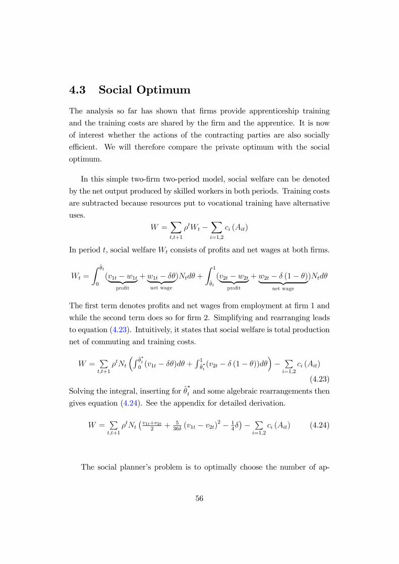
4.3 Social Optimum

The analysis so far has shown that �rms provide apprenticeship training

and the training costs are shared by the �rm and the apprentice. It is now

of interest whether the actions of the contracting parties are also socially

e¢ cient. We will therefore compare the private optimum with the social

optimum.

In this simple two-�rm two-period model, social welfare can be denoted

by the net output produced by skilled workers in both periods. Training costs

are subtracted because resources put to vocational training have alternative

uses.

W =Xt;t+1

�tWt �Xi=1;2

ci (Ait)

In period t, social welfare Wt consists of pro�ts and net wages at both �rms.

Wt =

Z �t

0

(v1t � w1t| {z }pro�t

+ w1t � ��| {z }net wage

)Ntd� +

Z 1

�t

(v2t � w2t| {z }pro�t

+ w2t � � (1� �)| {z }net wage

)Ntd�

The �rst term denotes pro�ts and net wages from employment at �rm 1 and

while the second term does so for �rm 2. Simplifying and rearranging leads

to equation (4.23). Intuitively, it states that social welfare is total production

net of commuting and training costs.

W =Pt;t+1

�tNt

�R ��t0(v1t � ��)d� +

R 1��t(v2t � � (1� �))d�

��Pi=1;2

ci (Ait)

(4.23)

Solving the integral, inserting for ��t and some algebraic rearrangements then

gives equation (4.24). See the appendix for detailed derivation.

W =Pt;t+1

�tNt�v1t+v2t

2+ 5

36�(v1t � v2t)

2 � 14��Pi=1;2

ci (Ait) (4.24)

The social planner�s problem is to optimally choose the number of ap-

56

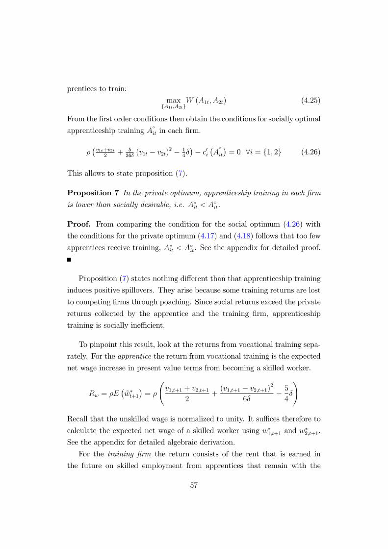
prentices to train:

maxfA1t;A2tg

W (A1t; A2t) (4.25)

From the �rst order conditions then obtain the conditions for socially optimal

apprenticeship training A�it in each �rm.

��v1t+v2t

2+ 5

36�(v1t � v2t)

2 � 14�� c0i

�A�

it

�= 0 8i = f1; 2g (4.26)

This allows to state proposition (7).

Proposition 7 In the private optimum, apprenticeship training in each �rmis lower than socially desirable, i.e. A�it < A�it.

Proof. From comparing the condition for the social optimum (4.26) with

the conditions for the private optimum (4.17) and (4.18) follows that too few

apprentices receive training, A�it < A�it. See the appendix for detailed proof.

Proposition (7) states nothing di¤erent than that apprenticeship training

induces positive spillovers. They arise because some training returns are lost

to competing �rms through poaching. Since social returns exceed the private

returns collected by the apprentice and the training �rm, apprenticeship

training is socially ine¢ cient.

To pinpoint this result, look at the returns from vocational training sepa-

rately. For the apprentice the return from vocational training is the expected

net wage increase in present value terms from becoming a skilled worker.

Rw = �E�~w�t+1

�= �

v1;t+1 + v2;t+1

2+(v1;t+1 � v2;t+1)

2

6�� 54�

!

Recall that the unskilled wage is normalized to unity. It su¢ ces therefore to

calculate the expected net wage of a skilled worker using w�1;t+1 and w�2;t+1.

See the appendix for detailed algebraic derivation.

For the training �rm the return consists of the rent that is earned in

the future on skilled employment from apprentices that remain with the

57

�rm. It arises as the worker�s marginal product exceeds the wage due to

frictions. Note that employment rents di¤er across �rms according to labor

productivity.

R1;f = �(v1;t+1 � v2;t+1 + 3�)

2

18�

R2;f = �(v2;t+1 � v1;t+1 + 3�)

2

18�

Private returns collected by the parties in each training contract are then

simply the sum of worker�s and �rm�s returns.

R1;priv = Rw +R1;f = �

5v1;t+1 + v2;t+1

6+4 (v1;t+1 � v2;t+1)

2

18�� 34�

!

R2;priv = Rw +R2;f = �

v1;t+1 + 5v2;t+1

6+4 (v1;t+1 � v2;t+1)

2

18�� 34�

!Social returns are given by

Rsocial = �

�v1;t+1 + v2;t+1

2+

5

36�(v1;t+1 � v2;t+1)

2 � 14�

�Finally, an externality of vocational education can be easily derived from

calculating the di¤erence between social and private returns, Xi = Rsocial �Ri;priv. Thus, the positive externality associated with an additional appren-

ticeship by each �rm is given by

X1 = �

�1

2� � (v1;t+1 � v2;t+1)

12�(v1;t+1 � v2;t+1 + 4�)

�

X2 = �

�1

2� � (v2;t+1 � v1;t+1)

12�(v2;t+1 � v1;t+1 + 4�)

�Proposition 8 Vocational training brings about a positive externality ontoother �rms. The externality decreases in �rm�s productivity, but increases in

opponent�s productivity and labor market frictions.

Proof. From comparative-static analysis follows @Xi@vi;t+1

< 0, @Xi@vj;t+1

> 0, and@Xi@�

> 0 for i; j = f1; 2g ; i 6= j.

58

The intuition for this result is straightforward. Because of wage competi-

tion among �rms, only a share of apprentices remain with the training �rm.

Put di¤erently, due to poaching of skilled workers, vocational training carries

a positive externality onto other �rms.

As an illustration, consider again the simple case of homogeneous tech-

nology. By setting v1;t+1 = v2;t+1 = vt+1, the expected return from appren-

ticeship training to an unskilled worker is simply

Rw = �

�vt+1 �

5

4�

�Likewise, �rms�returns from training an apprentice are

Rf = R1f = R2f = ��

2

Private returns of the apprentice and the �rm are therefore

Rpriv = Rw +Rf = �

�vt+1 �

3

4�

�Social returns are however

Rsocial = �

�vt+1 �

1

4�

�which clearly indicates a positive externality from training an apprentice.

X = X1 = X2 = ��

2

Intuitively, there is a return to vocational training that can neither be ob-

tained by the apprentice, nor the training �rm, but rather accrues to the

rival �rm. The opponent obtains a rent which arises because it can poach

some apprentices without being required to pay these skilled workers their

full marginal product. In the symmetric case this rent amounts to � �2. With

some returns from training remaining unconsidered by the private parties,

vocational training will be short of its socially e¢ cient level, A�it < A�it. Fig-

59

ure (4.3) summarizes this situation for the symmetric case with homogeneous

technology.

Figure 4.3: Social and Private Returns to Education

4.4 Discussion

In this simple model, due to costly labor market frictions, skilled workers

are inhibited from perfect wage arbitrage. Firms therefore possess some

monopsony power and obtain rents from employment. At the same time,

these labor market frictions cause some attachment of skilled individuals to

work for �rm i although a higher wage could be earned elsewhere. This

induces �rms not only to provide but also to partially �nance apprenticeship

training.

The model also predicts the existence of an externality from vocational

training. Rival �rms are able to reap positive spillovers from poaching work-

ers. While frictions cause some attachment of workers to the �rm, some

60

fraction still quits for another employer, thereby depriving the �rm of its

training investment. With training e¤orts distorted, then from a social point

of view too few apprenticeships are provided.

This model builds on a number of simplifying assumptions. Firstly, the

model is limited to only two periods. Secondly, apprenticeship training con-

sists of perfectly general skills with no �rm-speci�c element. Thirdly, appren-

tices and workers stay within the sector and there is no retirement. These

assumptions can be relaxed, altering the results quantitatively, but not qual-

itatively. See the appendix for a generalization with varying �rm positions

and chapter 6 for a generalization to an inde�nite number of �rms.

In the following chapters, emphasis will be put on the question whether

public policy possesses instruments to internalize the externality and thereby

to increase social welfare.

61

4.A Appendix

Proof of Proposition (1)Firms�wage o¤ers di¤er since their valuations for skilled workers vary.

Thus, the problem arises whether the respective wage o¤ers allow both �rms

to recruit skilled workers. This requires that ��t+1 > 0 and also 1� ��t+1 > 0.

Put di¤erently, conditions v1;t+1� v2;t+1+3� � 0 and v2;t+1� v1;t+1+3� � 0must be met. Some rearranging of both inequalities gives

v1;t+1 � v2;t+1 � �3� (4.27)

and

� (v1;t+1 � v2;t+1) � �3� () 3� � v1;t+1 � v2;t+1 (4.28)

One of these conditions will always be ful�lled. Clearly, the �rm with the

higher labor productivity will always be able to acquire skilled workers from

the labor market because it can o¤er higher wages. For the other condition

to hold (and also the second �rm to recruit workers from the labor market)

the productivity di¤erence is not to exceed the threefold of the commuting

cost rate. We assume this to be the case because we wish to analyze the

duopson case. From straightforward inspection of (4.9), (4.10), (4.11), and

(4.12) using conditions (4.27) and (4.28) then directly follows proposition

(1).

If both conditions were not met, the market for skilled labor would be a

monopson. Naturally, poaching cannot arise in a monopson. However, it is

a standard result that the monopson wage falls below the marginal product,

too.

Expected Future Net WageThe present value of a skilled workers future net income is represented by

the discounted expected net wage �E�~w�t+1

�when working for �rm 1 or 2.

E�~w�t+1

�=

Z ��t+1

0

�w�1;t+1 � ��

�d� +

Z 1

��t+1

�w�2;t+1 � � (1� �)

�d�

62

Dissolving the integral yields

E�~w�t+1

�=

�w�1;t+1� �

�

2�2��t+10

+

�w�2;t+1� � �� +

�

2�2�1��t+1

or

E�~w�t+1

�= w�1;t+1�

�t+1 �

�

2��2t+1 + w�2;t+1 � � +

�

2� w�2;t+1�

�t+1 + ��

�t+1 �

�

2��2t+1

which can be simpli�ed to

E�~w�t+1

�=�w�1;t+1 � w�2;t+1

��t+1 + ��

�t+1

�1� �

�t+1

�+ w�2;t+1 �

�

2

Inserting for ��t+1, w

�1;t+1, w

�2;t+1 and a couple of algebraic rearrangements

then yields

E�~w�t+1

�=v1;t+1 + v2;t+1

2+(v1;t+1 � v2;t+1)

2

6�� 54�

Proof of Proposition (3)Firm�s return from apprenticeship training is

Ri;f = �Ri;t+1 = �(vi;t+1 � vj;t+1 + 3�)

2

18�

Firm�s training incentives increase in labor market frictions since the partial

derivative with respect to � is positive.

@

@�Ri;f =

� (vi;t+1 � vj;t+1)2 + 9�2

18�2> 0

Note that the numerator denotes the familiar existence condition for both

�rms to be in the market.

Worker�s return from apprenticeship training is equal to the present value

of expected future net income.

Rw = �E ( ~wt+1) =v1;t+1 + v2;t+1

2+(v1;t+1 � v2;t+1)

2

6�� 54�

63

The partial derivative with respect to frictions is clearly negative, i.e. fric-

tions decrease worker�s training incentives.

@

@�Rw = �

6 (v1;t+1 � v2;t+1)2

6�� 54< 0

The sum of private returns of training at �rm i is given by

Ri;priv = �

�5vi;t+1 + vj;t+1

6+

4

18�(vi;t+1 � vj;t+1)

2 � 34�

�Again, the partial derivative with respect to frictions is clearly negative, thus

implying private training incentives to decrease in labor market frictions.

@

@�Ri;priv = �

72 (vi;t+1 � vj;t+1)2

(18�)2� 34< 0

Derivation of Equation (4.24)Welfare in this economy consists of the pro�ts and wages net of commuting

frictions.

Wt =

Z �t

0

(v1t � w1t + w1t � ��)Ntd� +

Z 1

�t

(v2t � w2t + w2t � � (1� �))Ntd�

Put simpler, welfare is net production.

Wt =

Z �t

0

(v1t � ��)Ntd� +

Z 1

�t

(v2t � � (1� �))Ntd�

By dissolving the integral

Wt = Nt

�v1� �

�

2�2��t0

+Nt

�v2� � �� +

�

2�2�1�t

obtain

Wt = Nt

�v1�t �

�

2�2

t + v2 � � +�

2� v2�t + ��t �

�

2�2

t

�

64


Wt = Nt

�v1�t � v2�t + ��t + v2 �

�

2� ��

2

t

�

Wt = Nt

��t

�v1 � v2 + � � ��t

�+ v2 �

�

2

�Inserting for �

�t

Wt = Nt

�v1 � v2 + 3�

6�

�v1 � v2 + � � �

v1 � v2 + 3�

6�

�+ v2 �

�

2

�

Wt = Nt

�v1 � v2 + 3�

6�� 5v1 � 5v2 + 3�

6+ v2 �

�

2

�Wt = Nt

�1

36�

�18�v1 � 10v1v2 + 5v21 + 5v22 + 18�v2 � 9�2

��then yields

Wt = Nt

�v1 + v22

+5

36�(v1 � v2)

2 � 14�

�From W =

Pt;t+1 �

tWt �P

i=1;2 ci (Ait) then follows equation (4.24).

Proof of Proposition (7)In order to show that social returns of apprenticeship training exceed the

private returns, compare the condition for the social optimum (4.26)

�

�v1 + v22

+5

36�(v1 � v2)

2 � 14�

�� c0i (Ai) = 0 8i = f1; 2g

with the conditions for the private optimum (4.17) and (4.18)

�(v1 � v2 + 3�)

2

18�� c01 (A1) = 0

and

�(v2 � v1 + 3�)

2

18�� c01 (A1) = 0

65

Consider �rst apprenticeship training at �rm 1. Social returns to training

will be above private returns if

v1 + v22

+5

36�(v1 � v2)

2 � 14� >

(v1 � v2 + 3�)2

18�

This simpli�es to

9� (v1 + v2) +5

2v21 � 5v1v2 +

5

2v22 �

9

2�2 > v21 � 2v1v2 + 6�v1� 6�v2 + v22 + 9�2

which gives

3�v1 + 15�v2 �27

2�2 > �3

2(v1 � v2)

2

or di¤erently

�9�2 + 2�v1 + 10�v2 + (v1 � v2)2 > 0

The last equation essentially states combinations of �, v1 and v2 for which

training will cause a positive or negative externality to arise. Moreover, from

above follows that both �rms are in the market if conditions (4.27) and (4.28)

are ful�lled. Inserting for (v1 � v2) we can rewrite to

�9�2 + 2�v1 + 10�v2 + 9�2 > 0

which then rearranges to

2�v1 + 10�v2 > 0

This condition is always ful�lled as long as commuting costs are positive.

Proceed likewise for apprenticeship training at �rm 2.

v1 + v22

+5

36�(v1 � v2)

2 � 14� >

(v2 � v1 + 3�)2

18�


9� (v1 + v2) +5

2v21 � 5v1v2 +

5

2v22 �

9

2�2 > v22 � 2v1v2� 6�v1 + 6�v2 + v22 + 9�2

66

and

15�v1 + 3�v2 �27

2�2 > �3

2(v1 � v2)

2

and �nally

10�v1 + 2�v2 + (v1 � v2)2 � 9�2 > 0

Again inserting for (v1 � v2) this condition is also ful�lled.

10�v1 + 2�v2 > 0

Extension for Varying Firm Locations and Market LengthThe exposition so far assumed a Hotelling street of unit length with �rms

located at either end. Yet, interval length as well as �rms�position may vary

freely. In order to assess this general case, denote the length of the interval

by I and the position of each �rm by �i. Figure 4.4 illustrates this extension.

Figure 4.4: Hotelling Street with Unspeci�ed Firm Location

67

Poaching PeriodThe arbitrage condition for the indi¤erent worker � is

w1;t+1 � �� 1

�= w2;t+1 � �

��2 � �

�Rearrange to obtain the equation for the indi¤erent worker that again marks

the share of workers to �rm 1.

� =w1;t+1 � w2;t+1

2�+�1 + �22

Accordingly, all workers in the interval�I � �

�will work for �rm 2. With

the workforce given we can write �rms wage setting problem.

maxfw1;t+1g

�1;t+1 = (v1;t+1 � w1;t+1) �(:)Nt+1

maxfw2;t+1g

�2;t+1 = (v2;t+1 � w2;t+1)�I � �(:)

�Nt+1

The �rst order conditions are now

� (w1;t+1 � w2;t+1)� � (�1 + �2) + (v1;t+1 � w1;t+1) = 0

�2�I + w1;t+1 � w2;t+1 + � (�1 + �2) + (v2;t+1 � w2;t+1) = 0

��(:) + (v1;t+1 � w1;t+1)1

2�= 0

��I � �(:)

�+ (v2;t+1 � w2;t+1)

1

2�= 0

which can be rearranged to the reaction functions

w�1;t+1 (w2;t+1) =1

2(v1;t+1 + w2;t+1 � � (�1 + �2))

w�2;t+1 (w1;t+1) =1

2(v2;t+1 + w1;t+1 � � (2I � (�1 + �2)))

68

Solving for the equilibrium wages then yields

w�1;t+1 =2

3v1;t+1 +

1

3v2;t+1 �

1

3� (2I + �1 + �2)

w�2;t+1 =1

3v1;t+1 +

2

3v2;t+1 �

1

3� (4I � �1 � �2)

For �1 = 0, �1 = 1, and I = 1 we obtain the equilibrium wages of the simple

case above. In addition, the general formulation allows to derive the e¤ects

of interval length and �rms�position: Equilibrium wages decrease the greater

the interval,@w�i;t+1@I

< 0. Intuitively, longer travels are costly and reduce wage

arbitrage.6 Note also that wage o¤ers by �rm 1 decrease the more both �rms

are located to the �right�of the interval,@w�1;t+1@�1

< 0 and@w�1;t+1@�2

< 0. Vice

versa, wage o¤ers by �rm 2 increase,@w�2;t+1@�1

> 0 and@w�2;t+1@�2

> 0.

From the equilibrium wages again follows the allocation of the workforce

��t+1 =

v1;t+1 � v2;t+1 + � (2I + �1 + �2)

6�

I � ��t+1 =

v2;t+1 � v1;t+1 + � (4I � �1 � �2)

6�

Equilibrium pro�ts in the future period from employing skilled workers

��1;t+1 =(v1;t+1 � v2;t+1 + � (2I + �1 + �2))

2

18�Nt+1

��2;t+1 =(v2;t+1 � v1;t+1 + � (4I � �1 � �2))

2

18�Nt+1

Training PeriodThe training decision is denoted by the maximization problem

argmaxfA1tg

��R�1;t+1Nt+1 � watA1t � ci (A1t)

argmaxfA2tg

��R�2;t+1Nt+1 � watA2t � ci (A2t)

6In this model, an increase in the length of the interval works essentially similar to an

increase in frictional cost parameter �.

69

The �rst order conditions with respect to the number of apprentices by each

�rm are now

�R�1;t+1 � wat � c0i (A1t) = 0

�R�2;t+1 � wat � c0i (A2t) = 0

Note that for �1 = 0, �1 = 1, and I = 1 we obtain the same training result as

in the simple case. Additionally, we learn that training increases in interval

length since@R�i;t+1@I

> 0. Intuitively, with a more segmented labor market,

�rms possess higher monopsony power. This allows for lower wages which in

turn enables to yield higher training returns. Note also that �rms�positions

on the interval a¤ect training outcomes. Since@R�1;t+1@�1

> 0 and@R�1;t+1@�2

> 0,

�rm 1 will train more apprentices, the more both �rms are located to the

�right� of the interval. Vice versa, �rm 2 will train less since its training

returns decrease,@R�2;t+1@�1

< 0 and@R�2;t+1@�2

< 0. This essentially states that if a

�rm has a strong position on the labor market, this will also lead to higher

training e¤orts.

70

Chapter 5

Incentive Schemes

The literature review in chapter 3 pointed to Pigou (1912) for having �rst

named poaching as the cause of underprovision of vocational training. Con-

cluding that training possesses additional social returns, he proposed to in-

troduce a system of �bounties and taxes�as a means to provide �rms with

additional training incentives. Training systems in several countries have

been build on this advise. This chapter will therefore take up this proposal

and analyze public policies for providing training incentives in further detail.

Policies to encourage employer training can be distinguished into volun-

tary arrangements and compulsory measures (Gasskov 1994, 8). Voluntary

training arrangements are private agreements among �rms, employer orga-

nizations and unions. The social partners thereby assume joint responsibil-

ity for vocational training. A common example are collective labor agree-

ments in Germany, which often include provisions for apprenticeship train-

ing. The joint training initiative (dt. Ausbildungspakt) of the federal govern-

ment and the confederation of employers�associations and training chambers

also falls into this category. Compulsory employer training, in contrast, de-

scribes training regulations from government intervention. Examples for such

mandatory measures include the regulation of training contracts, training

rules, or incentive schemes.

The focus of this section are incentive schemes. Besides training subsidies

or tax breaks, they can be of manifold form. In view of the policy debate in

71

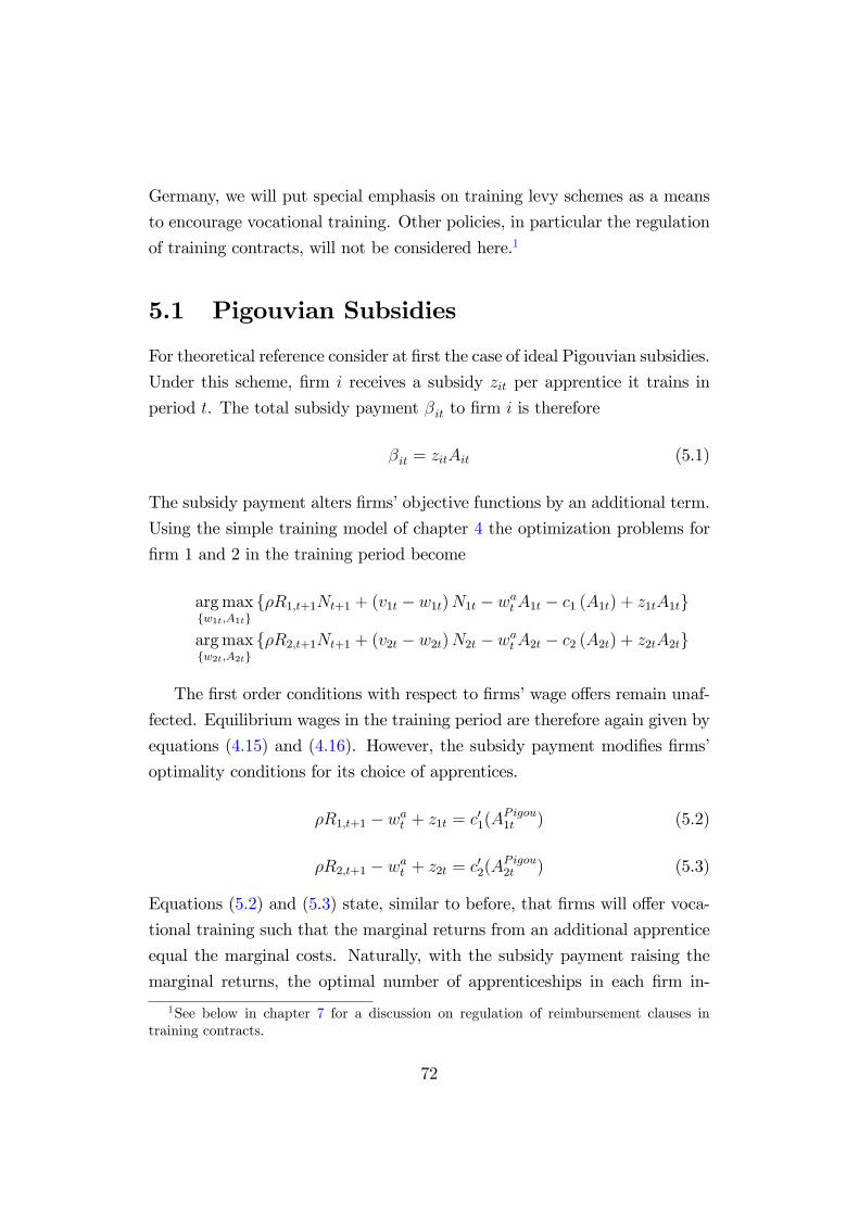
Germany, we will put special emphasis on training levy schemes as a means

to encourage vocational training. Other policies, in particular the regulation

of training contracts, will not be considered here.1

5.1 Pigouvian Subsidies

For theoretical reference consider at �rst the case of ideal Pigouvian subsidies.

Under this scheme, �rm i receives a subsidy zit per apprentice it trains in

period t. The total subsidy payment �it to �rm i is therefore

�it = zitAit (5.1)

The subsidy payment alters �rms�objective functions by an additional term.

Using the simple training model of chapter 4 the optimization problems for

�rm 1 and 2 in the training period become

argmaxfw1t;A1tg

f�R1;t+1Nt+1 + (v1t � w1t)N1t � watA1t � c1 (A1t) + z1tA1tg

argmaxfw2t;A2tg

f�R2;t+1Nt+1 + (v2t � w2t)N2t � watA2t � c2 (A2t) + z2tA2tg

The �rst order conditions with respect to �rms�wage o¤ers remain unaf-

fected. Equilibrium wages in the training period are therefore again given by

equations (4.15) and (4.16). However, the subsidy payment modi�es �rms�

optimality conditions for its choice of apprentices.

�R1;t+1 � wat + z1t = c01(APigou1t ) (5.2)

�R2;t+1 � wat + z2t = c02(APigou2t ) (5.3)

Equations (5.2) and (5.3) state, similar to before, that �rms will o¤er voca-

tional training such that the marginal returns from an additional apprentice

equal the marginal costs. Naturally, with the subsidy payment raising the

marginal returns, the optimal number of apprenticeships in each �rm in-

1See below in chapter 7 for a discussion on regulation of reimbursement clauses intraining contracts.

72

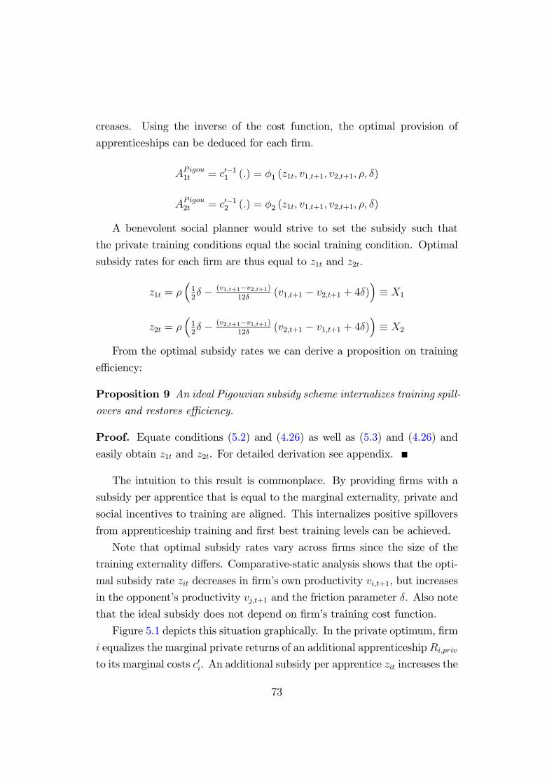
creases. Using the inverse of the cost function, the optimal provision of

apprenticeships can be deduced for each �rm.

APigou1t = c0�11 (:) = �1 (z1t; v1;t+1; v2;t+1; �; �)

APigou2t = c0�12 (:) = �2 (z1t; v1;t+1; v2;t+1; �; �)

A benevolent social planner would strive to set the subsidy such that

the private training conditions equal the social training condition. Optimal

subsidy rates for each �rm are thus equal to z1t and z2t.

z1t = ��12� � (v1;t+1�v2;t+1)

12�(v1;t+1 � v2;t+1 + 4�)

�� X1

z2t = ��12� � (v2;t+1�v1;t+1)

12�(v2;t+1 � v1;t+1 + 4�)

�� X2

From the optimal subsidy rates we can derive a proposition on training

e¢ ciency:

Proposition 9 An ideal Pigouvian subsidy scheme internalizes training spill-overs and restores e¢ ciency.

Proof. Equate conditions (5.2) and (4.26) as well as (5.3) and (4.26) andeasily obtain z1t and z2t. For detailed derivation see appendix.

The intuition to this result is commonplace. By providing �rms with a

subsidy per apprentice that is equal to the marginal externality, private and

social incentives to training are aligned. This internalizes positive spillovers

from apprenticeship training and �rst best training levels can be achieved.

Note that optimal subsidy rates vary across �rms since the size of the

training externality di¤ers. Comparative-static analysis shows that the opti-

mal subsidy rate zit decreases in �rm�s own productivity vi;t+1, but increases

in the opponent�s productivity vj;t+1 and the friction parameter �. Also note

that the ideal subsidy does not depend on �rm�s training cost function.

Figure 5.1 depicts this situation graphically. In the private optimum, �rm

i equalizes the marginal private returns of an additional apprenticeship Ri;privto its marginal costs c0i. An additional subsidy per apprentice zit increases the

73

marginal private returns such that the social optimum A�i can be achieved.

The Pigouvian subsidy thereby brings about a welfare gain that is equivalent

to the striped triangle.

Figure 5.1: Perfect Pigouvian Subsidy

Although an ideal Pigouvian subsidy possesses a strong theoretical ap-

peal for its ability to internalize positive spillovers, its premises are highly

unrealistic. In particular, the instrument requires to calculate subsidy rates

for vocational training at the �rm level. Because the externality arises from

poaching, the speci�c subsidy must be determined from �rms�future labor

productivity. This demands to gather and process very accurate and detailed

information on production as well as output market parameters, which would

already cause severe di¢ culties in practice. Additionally, and making matters

even worse, the interests of �rms and government to disclose the information

may strongly diverge. While the government seeks to obtain precise infor-

mation to assess the size of the externality, �rms have an interest to falsely

state their productivity levels in order to obtain larger subsidy payments.2

2More precisely, government faces asymmetric information with respect to �rms�pro-

74

Clearly, with only limited and inaccurate information available, the pos-

sibility to calculate �rm-speci�c subsidies is strongly reduced. Alternatively,

one may therefore consider to introduce a uniform subsidy that provides ad-

ditional training incentives on average for the economy or a particular sector.

Although this departs from the theoretical ideal, such an instrument could

be much simpler to determine and administer. It will now be analyzed.

5.2 Uniform Subsidies

Under a uniform subsidy scheme, government is constraint to a single subsidy

rate z. The total payment to �rm i for training apprentices thus becomes

�it = zAit (5.4)

As before, include the uniform subsidy in �rms� decision problem in the

training period. The optimality conditions for apprenticeship training are

now

�R1;t+1 � wat + z = c01(Auni1t ) (5.5)

�R2;t+1 � wat + z = c02(Auni2t ) (5.6)

Firms�optimal training levels Auni1t and Auni2t again increase in the subsidy

rate and can be determined from the inverse cost functions �i(:).

Auni1t = c0�11 (:) = �1 (z; v1;t+1; v2;t+1; �; �)

Auni2t = c0�12 (:) = �2 (z; v1;t+1; v2;t+1; �; �)

When introducing a uniform subsidy scheme, the government seeks to de-

termine the optimal subsidy rate z such that social welfareW (Auni1t (z); Auni2t (z))

is maximized. This uniform rate trades o¤ the disadvantages of insu¢ cient

and excessive subsidization. Using the social welfare function 4.24 and after

ductivity which cause a typical adverse selection problem to arise.

75

some simplications, the optimization problem of a benevolent government

can be stated by

argmaxfzg

( Pi=1;2

Auniit � ��v1;t+1+v2;t+1

2+ 5

36�(v1;t+1 � v2;t+1)

2 � 14��Pi=1;2

c0i�Auniit

�)

The �rst order condition (5.7) denotes the optimality condition for the welfare-

maximizing uniform subsidy rate z�.

Pi=1;2

@Auniit

@z��v1;t+1+v2;t+1

2+ 5

36�(v1;t+1 � v2;t+1)

2 � 14��Pi=1;2

c0i�Auniit

� @Auniit

@z= 0

(5.7)

For the optimal uniform subsidy rate z�, equation (5.7) states that the sum

of the marginal social returns from an increase in the subsidy rate is to equal

the sum of the marginal increases in the training costs. This allows to deduce

the next proposition.

Proposition 10 A uniform Pigouvian subsidy scheme, in contrast to an

ideal Pigouvian subsidy scheme, cannot achieve Pareto-optimality. At theoptimal subsidy rate z there will be over- and undertraining.

Proof. Rearrange the �rst order condition (5.7) and obtain

Pi=1;2

@Auniit

@z

��v1;t+1+v2;t+1

2+ 5

36�(v1;t+1 � v2;t+1)

2 � 14�� c0i

�Auniit

��= 0

Note that the term in the round brackets displays the social training con-

dition. In the Pareto-optimum, this term should equal zero for both �rms.

However, unless �rms were identical, the training cost functions and also the

number of apprentices vary across �rms. But with c0i(Auniit ) 6= c0j(A

unijt ), the

social training condition cannot be ful�lled and training therefore cannot be

e¢ cient.

Furthermore, because @Auniit

@z> 0, the whole condition equalizes to zero

only if the bracket term is positive for one �rm, and negative for the other.

This clearly implies that the optimal subsidy causes overtraining in one �rm

and undertraining in the other.

76

The intuition for this result is straightforward. Subsidization leads �rms

to increase training, but government is constraint to set a single subsidy rate.

Because the size of the training externality varies across �rms, the optimal

subsidy will exceed the ideal amount for the low externality �rm and fall

short of the ideal amount at the high externality �rm. Hence, the Pareto

optimal allocation cannot be achieved.

Figure 5.2 demonstrates this point graphically. Without a subsidy scheme,

�rms take A�1t and A�2t apprentices for training which equates the private

marginal returns R1;priv and R2;priv to the marginal training costs c0. Socially

optimal training at each �rm A�1t and A

�2t follows from the intersection with

Rsocial. An uniform subsidy z now raises the marginal returns to R1;priv + z

and R2;priv + z. This increases vocational training to Auni1t and Auni2t . How-

ever, since private training returns di¤er, there is undertraining in �rm 1,

Auni1t < A�1t, and overtraining in �rm 2, Auni2t < A

�2t.

Welfare e¤ects can also be displayed within the graph. The uniform

subsidy brings about welfare gains from increasing training above the pri-

vate level (striped areas). However, welfare losses from overtraining must

be substracted (shaded area). For the optimal uniform subsidy, the mar-

ginal social loss from overtraining equals the marginal social gain from larger

subsidization. Put di¤erently, this is equivalent to Rsocial � (R1;priv + z) =

� (Rsocial � (R2;priv + z)).

Because a uniform subsidy scheme cannot achieve �rst best training, this

instrument cannot restore Pareto-e¢ ciency. However, its introduction can

be shown to be Pareto-improving.3

Proposition 11 The introduction of a small uniform subsidy leads to a

Pareto-improvement.

Proof. At a subsidy rate of zero, the welfare function is increasing in z. Or,formally, @W

@zjz=0 > 0.

3For the distinction between Pareto-optimality and Pareto-improvement see Atkinson& Stiglitz (1980).

77

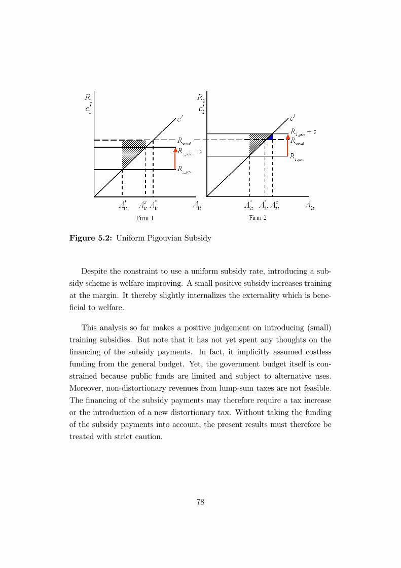
Figure 5.2: Uniform Pigouvian Subsidy

Despite the constraint to use a uniform subsidy rate, introducing a sub-

sidy scheme is welfare-improving. A small positive subsidy increases training

at the margin. It thereby slightly internalizes the externality which is bene-

�cial to welfare.

This analysis so far makes a positive judgement on introducing (small)

training subsidies. But note that it has not yet spent any thoughts on the

�nancing of the subsidy payments. In fact, it implicitly assumed costless

funding from the general budget. Yet, the government budget itself is con-

strained because public funds are limited and subject to alternative uses.

Moreover, non-distortionary revenues from lump-sum taxes are not feasible.

The �nancing of the subsidy payments may therefore require a tax increase

or the introduction of a new distortionary tax. Without taking the funding

of the subsidy payments into account, the present results must therefore be

treated with strict caution.

78

5.3 Training Levies

To this point, the analysis focussed on subsidy schemes to internalize spillovers

from vocational training. We now turn to training levies, which have received

much attention in Germany. Before analyzing the recent training levy pro-

posal, we �rst take a look at training levy schemes in general.

5.3.1 Policy Alternatives

The basic idea of training levies is to penalize �rms that do not train at all

or only to an insu¢ cient extent. These �rms are considered to bene�t from

positive spillovers and to free-ride on competitors�training e¤orts. Propo-

nents of training levy schemes claim that imposing training levies on these

�rms o¤ers additional training incentives and distributes training costs fairly

among �rms.

Training levies schemes have been introduced in several industrialized

countries. These schemes di¤er in scope, �nancing and institutional set-up.

Gasskov (1994), pp. 75¤., distinguishes the following variants:

� Revenue-generating levy schemes

� Levy-exemption schemes

� Levy-grant schemes

� Reimbursement schemes

Revenue-generating levy schemes impose a special compulsory tax on em-

ployers in order to fund major training programs. Training levies are usually

collected in proportion to workforce or payroll. The revenues, in contrast,

are spent on public or sectoral programs beyond the control of individual em-

ployers. Thus, revenue-generating levy schemes correspond closely to other

employment taxes collected from �rms since they generate revenues for public

training programs, but do not provide direct training incentives to �rms.

Levy-exemption schemes also impose a compulsory tax on workforce or

payroll. Its revenues are also spent on public training programs as in the

79

case of revenue-generating levy schemes. Additionally, however, there is an

exemption mechanism, which allows �rms to eliminate or reduce their levy

obligations if they provide training. The compulsory levy induces a min-

imum level of training expenses as employers possess strong incentives for

own training, both to reduce their levy obligation and to retain control on

spending. If �rms have better knowledge of training needs compared with

an administrative body, this exemption mechanism prevents misallocations

of training funds.

Levy-grant schemes di¤er from levy-exemption schemes in the withdrawal

of spending control. This scheme collects training levies from all �rms as be-

fore, but training grants are made subject to certain eligibility criteria. From

the view of training policy, this enables for some discretion. A levy-grant

scheme thus permits a greater redistribution of levy-based funds towards

�rms or sectors considered to be of particular importance. Note also that

levy-grant schemes require an administration which collects and redistributes

funds. This contrasts to levy-exemption schemes, which operate only in case

employer�s actions do not meet the training standard.

Reimbursement schemes entitle �rms for (partial) reimbursement of train-

ing expenditures if their training complies with the spending rules of the

training fund. Thus, these schemes are essentially subsidy programs. The

fund�s �nancial resources that are spent on reimbursement often result from

general tax receipts.

From this general classi�cation, let us discuss some actual training levy

schemes in industrialized countries.4 Revenue-generating levies are common

in countries with a strong public element in vocational education. In con-

trast, levy-exemption, levy-grant and reimbursement schemes are applied in

countries predominantly relying on on-the-job vocational training.

The literature often cites Britain as an example for levy-grant-schemes.

The British Training Act of 1972 introduced a levy-grant scheme at the

sectoral level to overcome market failure in �rm training. The scheme was

4For an international comparison on the �nancing of vocational training see in partic-ular Gasskov (1994) and Gasskov (2000). Greenhalgh (1999), Stevens (1999) and Bosch(2004b) also provide some account of training levies throughout the world.

80

however abandoned in favor for more market-oriented solutions in 1982.5

France applies a levy-exemption scheme both for vocational and contin-

uous education. In fact, it is considered to be the �rst country to have

introduced such a scheme on a national scale. Firms are levied a compulsory

payroll tax, but are exempt if their training expenses exceed this threshold

(Gasskov 1994, 86).6

An example of reimbursement schemes is Denmark. Unions and employ-

ers manage a training fund. It collects a general training levy from all �rms,

but reimburses for trainee wages (Bosch 2004a, 221).

5.3.2 German Levy Proposal

Let us now turn to the recent training levy proposal for Germany. Yet, it

must be emphasized that training levies have been proposed for many years.

In the late 1960s already, the federal government sought solutions in order

to react on shortages of apprenticeship training. Then as now, it considered

vocational education an area of utmost public responsibility and mandated

an expert commission to assess di¤erent policy instruments and come up with

a policy proposal. The commission emphasized the advantage of integrated

on-the-job training and schooling within the German dual system but it

also recognized important inequalities in �rms�e¤orts and activities towards

vocational training. As a remedy it proposed a training levy on all �rms to

feed funds for additional apprenticeship training Schulz (1972).

In the past, alike today, a training levy scheme was not universally ac-

cepted in the political landscape but eventually entered into legislation. The

training bill passed in 1976 mandated the federal government to raise a train-

ing levy if the demand for apprenticeships exceeds the supply by 12.5%. In

reality, however, the scheme was never implemented. A ruling of the fed-

eral constitutional court in 1980 overthrew the law on formal grounds, be-

cause the training law was passed without the approval of the federal council

5See Finegold & Soskice (1988) and Stevens (1999) for an account of vocational trainingpolicy in Britain.

6More detailed descriptions of the French system can be found in Gasskov (1994),Greenhalgh (1999) and Bosch (2004b).

81

Bundesverfassungsgericht (1980).7 Hereafter, training levy schemes vanished

from the political scene.8

The idea of training levies persisted within party manifests and union

activities. It reappeared recently in response to renewed shortages of ap-

prenticeship positions. This resulted into a federal law proposal that has

entered the formal legislative readings, but has been held in the federal par-

liament prior to the �nal vote. The issue whether to pass the law or not still

remains debated at present.9

If the bill were enacted in its present form, it would enable the federal

government to collect levies from �rms that train less than a certain stan-

dard and redistribute the revenues to �rms that exceed this standard. The

benchmark is a mandatory training quota that has been set to 7% of the

employed workforce. If a �rm falls short of this prescribed quota, it is to pay

a training levy, and if it exceeds the quota, it is eligible to additional funds.

Moreover, training levies and training grants increase the larger the devia-

tion from the benchmark level. The scheme thereby intends to discriminate

between varying training e¤orts across �rms.10

More precisely, �rms are entitled to a subsidy for every apprentice ex-

ceeding the training quota. Monthly subsidies per apprentice are to range

from e580 to e1240 depending on the profession. This variation is aimed

7According to the German constitution, bills concerning taxation and administrativeduties a¤ecting the federal states are subject to vote by the federal council, Germany�supper legislative chamber representing the federal states.

8Although the introduction of a training levy scheme by federal law had failed, suchschemes have been introduced at the sectoral level. In 1975, the social partners in theconstruction industry negotiated a collective agreement which set-up a levy-grant schemefor vocational training in this sector. This agreement has been declared generally bindingand is therefore valid for all �rms in this sector. The scheme collects a training levy of1.6% on �rms�payroll and redistributes the money according to �rms� training e¤orts.In the �rst year, a �rm receives a grant amounting to the tenfold of a monthly trainingallowance. In the second year, the payment shrinks to the sixfold, and in the third yearto the singlefold. Some authors consider this scheme to be examplary as the trainee ratehas since increased (Bosch 2004a, 222).

9For the legislative status, the precise text of the law and an explanatory statement tothe legislative intentions see in particular Deutscher Bundestag (2004).10For details to the law proposal see the draft in Deutscher Bundestag (2004), in par-

ticular §§9-11 BerASichG.

82

to re�ect trainee wages that di¤er strongly across occupations. In contrast,

�rms are levied a certain penalty per employee if the training quota is not

attained.11 Other than the subsidy rate and the mandatory training quota,

the law proposal leaves the penalty rate unspeci�ed. Instead, it is to be de-

termined such that the whole scheme is self-�nancing, i.e. that subsidies and

administrative expenses can be �nanced.

In order to allow for a detailed economic analysis, we now transform this

proposal into formal terms. Let �it again be the payment to �rm i resulting

from the scheme in the training period. Moreover, let �it de�ne the training

quota of �rm i, i.e. �rm�s ratio of apprentices to employees.

�it =AitNit

(5.8)

De�ne � to be the mandatory training quota that speci�es the desired train-

ing standard. Now, if a �rm falls short of the mandatory level, i.e. �it < �,

the �rm has to pay a penalty p for every skilled worker it employs. Because

the penalty intends to re�ect di¤erences in training across �rms, the total

levy decreases for every apprentice the �rm trains. Accordingly, the work-

force that would be equivalent to the actual number of apprentices at the

mandatory training quota, i.e. N = Ait�, is deducted from the levy base.

Training levies to �rm i are thus calculated according to

levyit = ��Nit �

Ait�

�� p

By contrast, if a �rm exceeds the mandatory level, i.e. �it > �, the �rm

receives a grant z per apprentice it trains above the mandatory training

11The law de�nes apprentices as those trainees employed by a �rm that fall under theconditions of the apprenticeship training law. Employees are full-time workers that aresubject to social insurance contributions. Thus, the law excludes interns, student appren-tices, freelance workers, temporary workers and so-called minor employments. Therebysome substitution between di¤erent trainee and worker categories may arise resulting indistortions from the levy-grant scheme. These issues are however neglected here.

83

level. The training grant to �rm i is thus

grantit = (Ait � �Nit) � z

Equation (5.9) summarizes the payment to �rm i resulting from the proposed

training levy scheme.

�it =

8><>:��Nit � Ait

�

�� p

(Ait � �Nit) � z0

if

�it < �

�it > �

�it = �

9>=>; (5.9)

Factoring out Nit and using (5.8) to replace for �rm�s training quota then

leads to

�it =

8><>:(�it � �) � p

�Nit

(�it � �) � zNit

0

if

�it < �

�it > �

�it = �

9>=>; (5.10)

For analytical simplicity, let us assume �rms are given the same �nancial

incentive for an additional apprentice, regardless of whether the �rm exceeds

or falls short of the training quota. Then, as follows from (5.10), penalty and

subsidy must obey the relation p�= z or p = z�.12 The net payment thereby

simpli�es to

�it = (�it � �) zNit (5.11)

Note the close similarity of equation (5.11) to an incentive scheme for the pri-

vate provision of public goods discussed in Falkinger (1996), which proposes

to punish or reward deviations from the average contribution level.

When replacing for the training quota in equation (5.11), the scheme can

be split up into two parts. One term depends on the number of apprentices,

the other on the number of employees.

�it = zAit � z�Nit (5.12)

12This assumption could be justi�ed on e¢ ciency grounds because otherwise an addi-tional redistributive element would be introduced into the scheme.

84

For notational ease de�ne the tax rate � , � � z�. The payment term then

simpli�es to �it = zAit� �Nit whereby it becomes evident that �rms receivea uniform subsidy z per apprentice and pay a tax � per employee. This

directly leads to the following conclusion.

Proposition 12 The proposed training levy scheme corresponds to a tax-subsidy-system. It subsidizes apprenticeship training and raises an additional

employment tax.

Proof. Obvious.

Despite their apparent similarity, there are nevertheless notable di¤er-

ences between tax-subsidy-systems and levy-grant-systems. Under a tax-

subsidy-system, an economic agent is paying taxes as well as receiving sub-

sidies for providing a bene�cial activity. All monetary �ows pass through

the public budget. Under a levy-grant-system, by contrast, the agent only

exchanges a net payment with the public budget, i.e. a levy amount net of

any subsidies. The transaction volume is therefore much smaller. Essentially,

levy-grant-systems possess the feature of central clearing while tax-subsidy-

systems do not. This property can bring about some savings in administra-

tion, collection, and payment transactions (Falkinger 1996, 414). However,

as our analysis completely neglects administrative costs, these di¤erences are

not taken up further.

The proposed levy scheme is self-�nancing only if the budget balances.

This is the case when all levies raised equal grants and administrative ex-

penses. Assume the scheme to work without any cost.13 The budget con-

straint is thus given by

Pi

�it =Pi

(�it � �) � zNit =Pi

zAit �Pi

�Nit = 0 8t (5.13)

From equation (5.13) we can infer the next proposition.

13Of course, this is not an innocuous assumption. It is made here for expositionalpurposes. Below the analysis reconsiders the issue of administrative costs more explicitly.

85

Proposition 13 The budget of the training levy scheme balances if the manda-tory training quota is set to equal the average training quota.

Proof. From (5.13) follows that the budget balances forP

i (�it � �)�zNit =

0. This can be rearranged toP

i �itNit = �P

iNit which then leads to

� =Pi AitPiNit

� ��.

Intuitively, by setting the mandatory training quota to equal the average

quota, the budget will automatically be equalized as training below and above

this standard will reciprocally balance.

5.3.3 Private Optimum

Given these general remarks on the training levy proposal, let us now inves-

tigate how �rms�training decisions are a¤ected from an introduction of this

scheme. The optimization problems for �rm 1 and 2 are again altered in the

training period.

argmaxfw1t;A1tg

f�R1;t+1Nt+1 + (v1t � w1t � �)N1t � watA1t � c1 (A1t) + zA1tg

argmaxfw2t;A2tg

f�R2;t+1Nt+1 + (v2t � w2t � �)N2t � watA2t � c2 (A2t) + zA2tg

The optimality conditions for training are identical to equations (5.5)

and (5.6). Thus, as in the case of uniform subsidies, the optimal number of

apprentices increases in the subsidy z. The optimality conditions for �rms�

wage o¤ers w1t and w2t in contrast are given by (5.14) and (5.15). As before,

they denote a pair of reaction functions.

� 2w1t + w2t � � � � + v1t = 0 (5.14)

� 2w2t + w1t � � � � + v2t = 0 (5.15)

Again solving for the Hotelling-Nash-equilibrium then allows to derive the

equilibrium wages wlevy1t and wlevy2t .

wlevy1t =2

3v1t +

1

3v2t � � � � (5.16)

86

wlevy2t =1

3v1t +

2

3v2t � � � � (5.17)

Proposition 14 The employee tax to �nance the training subsidies is fullyshifted onto workers.

Proof. This follows from (5.16) and (5.17) with @wlevyit

@�= �1.

The intuition for this result can be put as follows: The employee tax

decreases the value product that a �rm can earn from employing skilled

workers. Firms will therefore reduce their wage o¤er by this amount. The

training levy scheme thus burdens skilled workers employed in the training

period and leaves �rms�pro�ts una¤ected.

It must be noted, however, that this proposition results from the assump-

tions on the production function. Assuming an exogenous and constant labor

productivity considers the output market to be perfectly competitive, such

that the employee tax cannot be shifted onto consumers by increasing prices.

Moreover, with labor as the only input, tax shifting resulting from substitu-

tion e¤ects is excluded.

5.3.4 Social Optimum

So far, the training levy scheme was revealed to provide additional training

incentives by paying out a uniform subsidy z that is �nanced from an em-

ployment tax � = z� on all �rms. It has two immediate e¤ects. Firstly, the

subsidy encourages additional apprenticeship training. Similar to the uniform

subsidy scheme, marginal training returns increase for all �rms. Secondly,

the employment tax reduces the wage o¤ers to the present skilled workforce.

Thus skilled work becomes less attractive in comparison to alternative in-

come sources. In the training period, labor supply will therefore decrease

and production output will shrink.

When deciding on introducing the levy scheme, a rational and benevolent

government will trade o¤ the welfare gains from additional training against

the welfare losses for the present workforce. It is additionally constraint to

87

a balanced budget. Aiming to determine the optimal subsidy and tax rates,

the government�s decision problem can be displayed by

maxfz;�g

W =Pt=1;2

�t�1Wt �Pi=1;2

ci(Alevyit )

s.t.Pi=1;2

�zAlevyit � z�Nit

�= 0

This constrained maximization problem can be solved using the Lagrangian

method.

maxfz;�g

L =Pt=1;2

�t�1Wt �Pi=1;2

ci(Alevyit )� �

Pi=1;2


�The �rst order conditions are

@L@z

=Pt=1;2

�t�1 @Wt

@z�Pi=1;2

c0i@Alevyit

@z� �

Pi=1;2

�z@Alevyit

@z� z�@Nit

@z

�= 0

@L@�

=Pt=1;2

�t�1 @Wt

@��

Pi=1;2

��zNit � z�@Nit

@�

�= 0

@L@�

=Pi=1;2


�= 0

Merging these conditions, the optimal subidy rate and mandatory training

quota can be solved for. The optimality condition (5.18) links all optimal

values of z� and ��.

Pt=1;2

�t�1

0@@Wt

@z+ @Wt

@�

Pi=1;2

�@Alevyit

@z� �@Nit

@z

�P

i=1;2

�Nit + �@Nit

@�

�1A =

Pi=1;2

c0i@Alevyit

@z(5.18)

Also address the question whether the introduction of the training levy

scheme would be welfare-improving. From the balanced budget constraint

(5.13) follows that the mandatory training quota cannot be set independently,

but depends positively on the subsidy rate chosen. The higher the subsidy,

the higher the training quota is to be set. Formally we have �(z) with �0 > 0.

Using the budget constraint in this implicit form, the welfare problem can be

88

rewritten as W (z; �(z)). The total di¤erential with respect to the subsidy

rate is stated in equation (5.19).

dW

dz=Pt=1;2

�t�1�@Wt

@z+ @Wt

@�@�@z

��Pi=1;2

c0i@Alevyit

@zR 0 (5.19)

Proposition 15 The introduction of a levy-grant-scheme can be ambiguousto welfare.

Proof. If the total di¤erential were positive for z = 0, dWdzjz=0 > 0, the

introduction of the levy scheme would be welfare-improving. Equation (5.19)

consists of three terms. The �rst term represents the discounted welfare gain

of training brought about by a subsidy. The second term depicts the welfare

loss resulting from the levy. It is negative since @Wt

@�< 0 and @�

@z> 0. The

third term states the marginal cost of additional training, which must be

deducted from welfare when training incentives are introduced. The overall

results is thus ambiguous since the total di¤erential cannot be signed without

speci�c functional forms.

The proposition essentially states that the welfare e¤ects from introducing

a levy scheme for apprenticeship training cannot be determined theoretically.

Whether this scheme would be bene�cial or detrimental to the economy�s wel-

fare critically depends on �rms�training reaction to the subsidy and workers�

change in labor supply. An empirical assessment of the training and labor

supply elasticities would therefore be required to determine net welfare.

5.4 Discussion

The model of the previous chapter demonstrated that apprenticeship training

exhibits positive spillovers on other �rms in imperfect labor markets. Public

policies addressing this problem and increasing training e¤orts are therefore

of interest. This chapter analyzed various �scal instruments that introduce

incentives for vocational training.

It was shown that an ideal Pigouvian subsidy could, at least in theory,

89

restore the social optimum. For this to be the case the subsidy should depend

on future productivity levels of both training and competing �rms. In reality,

however, this information may not be available. Thus, the use of an uniform

subsidy may be required. In comparison to the ideal Pigouvian scheme it will

bring about additional distortions. Because a uniform rate cannot account

for di¤erences between �rms, such a training subsidy scheme may lead to

undertraining in some �rms and overtraining in others. Nevertheless, we

were able to demonstrate that introducing a small uniform subsidy would be

welfare-improving if non-distortionary funding were available.

This chapter also investigated the widespread proposal of training levies.

It was unveiled that such schemes are a particular form of tax-subsidy-

systems. A tax is levied on employment and a subsidy is paid per apprentice-

ship. The analysis furthermore showed this tax, although paid by the �rm,

to be fully shifted onto workers in the form of lower wages. This outcome

is however an artifact of the model. If also output markets are imperfectly

competitive, some tax shifting onto consumers may occur.

Our analysis of the levy scheme predicts a decrease in labor supply and

output if the tax is at least partially shifted onto workers and labor supply

is somewhat elastic. A training levy thus brings about welfare gains from

subsidizing apprenticeship training and simultaneously causes welfare losses

from lower output due to reduced labor supply. The net welfare e¤ect was

shown to be theoretically ambiguous, thus requiring an empirical estimation.

Additionally, since no administrative costs have been taken into account

so far, this analysis requires some caution. Clearly, there are costs to ad-

minister, monitor and verify the subsidy scheme, that arise both for the

government as for �rms. In particular, non-negligible costs are associated

with the collection and distribution of funds as well as with the gathering

and processing of the necessary information. Once these costs are included,

they are an additional detriment on welfare.

90

5.A Appendix

Derivation of the Perfect Pigouvian SubsidyTo attain the social optimum A�it(z) = A

�it must hold. For �rm 1 set

conditions (5.2) and (4.26) equal:

�R1;t+1 � wat + z1 = �Rsocial

Recall that wat = ��E ( ~wt+1) = �Rw. Thus z1t can be rearranged to

z1t = � (Rsocial �R1;t+1 �Rw)

Inserting for Rsocial, R1;t+1 and Rw and simplifying then yields the optimal

subsidy to �rm 1.

z1t = ��12� � (v1;t+1�v2;t+1)

12�(v1;t+1 � v2;t+1 + 4�)

�� X1

Proceed likewise for �rm 2 and obtain the optimal subsidy rate z2t.

z2t = ��12� � (v2;t+1�v1;t+1)

12�(v2;t+1 � v1;t+1 + 4�)

�� X2

91

Chapter 6

Generalized Model ofVocational Training

Vocational training has so far been analyzed within a simpli�ed two-�rm

two-period model. This chapter now generalizes the model by allowing for

an inde�nite number �rms. It thereby re�ects reality a bit closer. Moreover,

it enables to study the e¤ects of varying labor market competition on the

provision and �nancing of vocational training.

6.1 Model Set-up and Assumptions

In comparison to above, model set-up and assumptions di¤er only slightly.

Instead of a linear Hotelling-street consider now a Salop-circle with length

again normalized to unity.1 Let there be n �rms which are located evenly

across the economic space. The position of a �rm can therefore be denoted

by qi = i�1nfor all i = f1:::ng. Figure (6.1) depicts this situation for the case

of 4 �rms.

As before, assume workers to be homogeneous in skills, but to vary in

location. This is represented by the di¤erentiation parameter � which is dis-

tributed uniformly across the unit interval. Workers again incur commuting

1This model is originally due to Salop (1979). See also the common textbook presen-tations in Tirole (1988), pp. 282¤., and Bester (2004), pp. 124¤.

92

Figure 6.1: Salop Circle for n = 4

costs in order to work for a �rm. These costs increase in the distance between

the worker and the �rm at the linear rate �. The net wage of worker � when

working for �rm i can therefore be denoted by equation (6.1).

~wit (witj�) = wit � � jqi � �j (6.1)

Taking these modi�cations into account, let us again solve this two-stage

game using backward induction. Similar to above, we will �rst consider the

private optimum and then turn to the social optimum.

6.2 Private Optimum


Consider at �rst the poaching period t + 1. Firms strive to attract skilled

workers by making appropriate wage o¤ers wi;t+1. Workers, on the other

hand, aim for a high wage income net of commuting costs. They will choose

to work for the �rm yielding the highest net wage ~wi;t+1. Consequently,

the allocation of the workforce depends on �rms�wage o¤ers and workers�

locations.

93

A worker will decide between the wage o¤ers of his two neighboring �rms.

Let �i;i+1 be the worker in the interval [qi; qi+1] who is indi¤erent between

working for �rm i or �rm i + 1 in this period. For this worker net wages of

working at either �rm are equal and, therefore, the arbitrage condition (6.2)

is ful�lled.

wi;t+1 � ��i;i+1 � qi

�= wi+1;t+1 � �

�qi+1 � �i;i+1

�(6.2)

Simplifying and rearranging the arbitrage condition allows to obtain the in-

di¤erent worker �i;i+1 as a function of �rms�wage o¤ers wi;t+1 and wi+1;t+1.

�i;i+1 =(qi+1 + qi)

2� (wi+1;t+1 � wi;t+1)

2�

Likewise, equations for indi¤erent workers between all other �rms are ob-

tained. Now, all workers in the intervalh�i�1;i; �i;i+1

iwill choose to work for

�rm i. The share of the skilled workforce that is employed by the �rm in this

period can thereby be denoted by

i;t+1 =

Z �i;i+1

�i�1;i

f (�) d�

For simplicity workers are assumed to be uniformly distributed along the

Hotelling-circle, f (�) = 1. Thus, �rm�s share in the workforce can be deter-

mined by

i;t+1 = �i;i+1� �i�1;i =qi+1 � qi + qi � qi�1

2+(2wi;t+1 � wi�1;t+1 � wi+1;t+1)

2�

Recall that �rms are located evenly across the economy. The distance be-

tween two �rms is4q = qi+1�qi = i+1�1n� i�1

n= 1

n. Therefore, i;t+1 reduces

to

i;t+1 =1

n+1

2�(2wi;t+1 � wi�1;t+1 � wi+1;t+1) (6.3)

Intuitively, equation (6.3) states that �rm i�s recruitment of skilled work-

ers increases in its own wage o¤er, but decreases in the wage o¤ers of the

neighboring �rms.

94

Firms derive pro�ts from the excess of worker�s marginal product over

wages paid to the employed workforce, �i;t+1 = (vi;t+1 � wi;t+1) i;t+1Nt+1.

In order to maximize pro�ts, �rms strive to post appropriate wage o¤ers.

On the one hand, wages are a costly input that reduces pro�ts. On the other

hand, wages are a means to attract a larger fraction of the skilled workforce

and thereby increase pro�ts. Firm i�s optimization problem in the poaching

period is thus

maxwi;t+1

�i;t+1 = (vi;t+1 � wi;t+1)

�1

n+1

2�(2wi;t+1 � wi�1;t+1 � wi+1;t+1)

�Nt+1

(6.4)

Equation (6.5) displays the �rst order condition with respect to wi. The

second order condition for a local maximum is satis�ed with @2�i;t+1@wi;t+1

= �2�<

0.

� 1

n� 1

2�(2wi;t+1 � wi�1;t+1 � wi+1;t+1) +

1

�(vi;t+1 � wi;t+1) = 0 (6.5)

Proceeding likewise for all �rms i = f1:::ng results into a system of n linear

equations. They denote the wage reaction functions, i.e. �rm�s optimal wage

o¤er given the wage o¤ers by the neighboring �rms.

1

2vi;t+1 � wi;t+1 +

1

4wi�1;t+1 +

1

4wi+1;t+1 �

�

2n= 0 8i = f1:::ng (6.6)

For the purposes of this analysis, consider only the case of identical tech-

nology across �rms. With homogeneous productivity, vi;t+1 = vj;t+1 = vt+1,

�rms�wage o¤ers will also be identical, wi;t+1 = wj;t+1 = wt+1.2 The prevail-

ing market wage in this period can thus be determined by (6.7)

w�t+1 = vt+1 ��

n(6.7)

This allows to state the next proposition:

2In the case of heterogeneous productivity, alike the two-�rm setting above, the issuearises whether all �rms are actually able to recruit workers from the labor market. Firmspossessing an inferior production technology can naturally only post lower wage o¤ers. Inthe case of an interior solution, there will be no uniform market wage. Instead, wages willdi¤er across �rms according to labor productivity.

95

Proposition 16 Firms�equilibrium wage o¤ers to skilled workers fall belowthe marginal product of labor, w�t+1 < vt+1.

Proof. Inspection of (6.7) directly shows w�t+1 < vt+1 for � > 0 and n > 0.

Note that this result essentially restates proposition (1) for the case of

n �rms. Labor market frictions again inhibit workers from perfect wage

arbitrage. This lends some wage-setting power to �rms such that in equi-

librium the wage is below the marginal product of labor. In fact, higher

frictions reduce worker turnover and increase the monopsony power of �rms.

Correspondingly, comparative-static analysis shows the equilibrium wage to

decline in the commuting rate �. Moreover, with respect to the number of

�rms, the following proposition can be made.

Proposition 17 The market wage increases in the number of �rms com-peting for skilled labor. Furthermore, on perfectly competitive labor markets,

wages equal the marginal product of labor, w�t+1 = vt+1.

Proof. From (6.7) obtain@w�t+1@n

> 0 and limn!1

w�t+1 = vt+1.

Intuitively, the more �rms strive to recruit skilled workers, the more com-

petitive is the labor market. This drives up workers�wages to the marginal

product of labor.

With wages below the marginal product, �rms will consequently earn

employment rents. For the symmetric case under consideration, �rms�equi-

librium pro�ts in the poaching period can be determined according to

��i;t+1 = ��j;t+1 =�vt+1 � w�t+1

� �t+1Nt+1 =

�

n2Nt+1 (6.8)


Now consider the training period t. In this period, just as in the poaching

period, �rms compete for skilled workers by making appropriate wage o¤ers.

Additionally, �rms can decide to take apprentices for training.

96

In the training period, �rm i�s recruitment of skilled workers again de-

pends on its own wage o¤er and on wage o¤ers by neighboring �rms. As

before, �rm�s workforce can be determined by using the arbitrage condition

of the indi¤erent worker. Thus, analogous to equation (6.3), �rm i�s share of

the existing workforce in the training period, it, can be denoted by (6.9).

it =1

n+1

2�(2wit � wi�1;t � wi+1;t) (6.9)

In the training period, a �rm�s optimization problem consists of dis-

counted future pro�ts and present pro�ts from employment minus any wages

to apprentices and training costs, ��i;t+1+�it�waAit� ci (Ait). Firms striveto maximize pro�ts by optimally choosing their wage o¤er wit and the number

of apprentices Ait to take for training.

argmaxwit;Ait

��

n2Nt+1 + (vit � wit) itNt � waAit � ci (Ait)

�The �rst order conditions are

@

@wit= � 1

n� 1

2�(2wit � wi�1;t � wi+1;t) +

1

�(vit � wit) = 0 (6.10)

@

@Ait= �

�

n2� wa � c0i (A

�it) = 0 (6.11)

where second order conditions are ful�lled with @2

@wit< 0 and @2

@Ait< 0.

At �rst, analyze the �rst order condition with respect to �rm�s wage o¤er.

Equation (6.10) states �rm i�s wage reaction function for the training period.

Given the wage reaction functions of all �rms and assuming homogeneous

productivity as in the poaching period, the equilibrium wage for skilled labor

in the training period can be determined by (6.12).

w�t = vt ��

n(6.12)

97

Equation (6.11) displays the �rst order condition with respect to the num-

ber of apprentices. It provides �rm i�s optimality condition for apprenticeship

training equating the returns of an additional apprentice to the apprentice

wage and the marginal training costs. Again, we can infer the apprentice

wage from the participation constraint. Apprentices are willing to forego

earnings in the training period that correspond to the increase in the ex-

pected future net wage, �wa � �E( ~wt+1). After solving for the expected net

wage, apprentices�pay can be determined from equation (6.13).

� wa = �E( ~wt+1) = �

�vt+1 �

5

4

�

n

�(6.13)

See the appendix for a detailed derivation of the expected net wage. Recall

that condition (6.13) assumes the wage of unskilled workers to be normalized

to zero and all bargaining power in the apprenticeship contract to be with

the training �rm. Inserting the apprentices�wage into the training condition,

the optimality condition for apprenticeship training becomes

�

��

n2+ (vt+1 �

5

4

�

n)

�= �

�vt+1 �

n� 1n

�

n� �

4n

�= c0i (A

�it) (6.14)

Using the inverse of the cost function we can infer �rm i�s optimal number

of apprenticeships.

A�it = c0�1i (:) = �i (vt+1;�; n; �)

Proposition 18 In the private optimum, a �rm will provide A�it apprentice-ships. Although vocational training is characterized as perfectly general, �rms

will partially carry its costs.

Proof. This follows from (6.14) where � �n2> 0, �E( ~wt+1) > 0 and c0i > 0.

With labor market frictions inhibiting wage arbitrage and slowing worker

turnover, �rms can expect to earn some rents from employing workers they

have previously trained. Thus, in contrast to conventional human capital

theory, this model proposes �rms not only to provide and but also to partially

�nance costly apprenticeships.

98

Proposition 19 The share in training costs borne by the training �rm de-

creases in labor market competition. Moreover, on perfectly competitive labor

markets, all costs of vocational training are �nanced by the apprentice.

Proof. Apply the implicit function theorem on (6.14).

This proposition restates Becker�s famous result. On competitive labor

markets, �rms cannot obtain any returns from general training. However,

with wages being equal to the marginal product of labor, workers reap the

full returns from vocational training.

6.3 Social Optimum

The previous section essentially restated the results of the two-�rm setting

for the n-�rm model. The analysis pointed out that �rms provide apprentice-

ship training, but training costs are shared by the �rm and the apprentice

depending on the competition on the labor market. This section now inves-

tigates welfare implications of training. It will be asked whether the training

choices by the private parties are also socially e¢ cient.

Social welfare consists of the net output produced by skilled workers in

both periods reduced by resources spent on training.

W = �Wt+1 +Wt �nPi=1

ci (Ait) (6.15)

Net output in period t can be determined from the following integral over

workers which denotes output minus commuting costs.

Wt =

Z 1

0

(vt � (�; n)) f (�)Ntd� (6.16)

Dissolving the integral and inserting above then allows to state social welfare

(6.17). See the appendix for a complete derivation.

W =Pt;t+1

�t�1�vt �

�

4n

�Nt �

nPi=1

ci (Ait) (6.17)

99

A benevolent social planner aims to maximize social welfare by optimally

choosing �rms�training levels. Socially optimal training can be derived from

condition (6.18) which equates the marginal social return to training to the

marginal training cost.

�

�vt+1 �

�

4n

�� c0i(A

oit) = 0 (6.18)

Proposition 20 Apprenticeship training is socially ine¢ cient as private op-timal training is short of the social optimum, A�it < A

�it.

Proof. Compare conditions (6.14) and (6.18). Note that the social trainingreturns exceed private returns, �

�vt+1 � �

4n

�> �

��n2+ vt+1 � 5

4�n

�. With

increasing training costs, c0i > 0; then immediately follows A�it > A�it.

The intuition to this result is similar to above. Apprenticeship training

brings about positive spillovers to other �rms. With social returns exceeding

the private returns, the private provision of vocational training will be socially

ine¢ cient.

Let us again illustrate this result by pointing out the returns from voca-

tional training separately for all parties involved. The return from vocational

training for apprentices is the expected increase in the net wage by becoming

a skilled worker.

Rw = �E ( ~wt+1) = �

�wt+1 �

�

4n

�= �

�vt+1 �

5

4

�

n

�Returns to the training �rm result from labor market frictions. As workers

do not react to small wage di¤erentials, �rms enjoy some monopsony power

and the equilibrium wage is reduced below the marginal product of labor.

Thus, from employing former apprentices as skilled workers �rms will earn a

rent that can be used to cover training costs.

Rf = �1

n

�

n

100

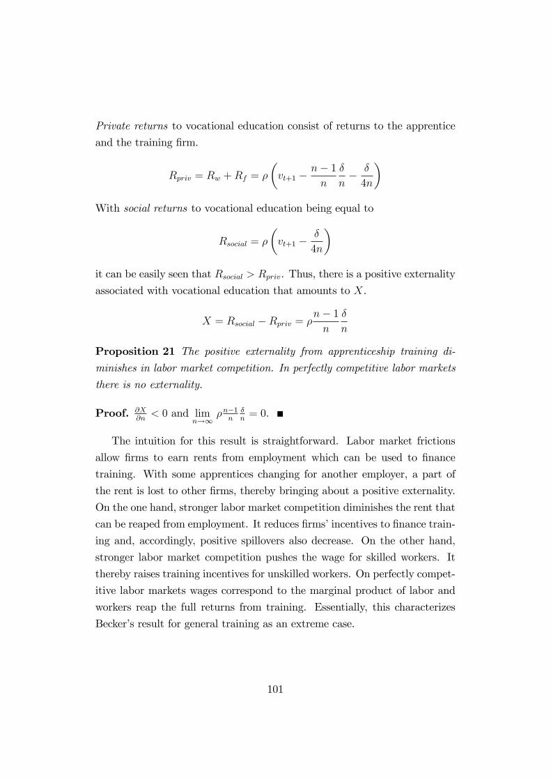
Private returns to vocational education consist of returns to the apprentice

and the training �rm.

Rpriv = Rw +Rf = �

�vt+1 �

n� 1n

�

n� �

4n

�With social returns to vocational education being equal to

Rsocial = �

�vt+1 �

�

4n

�it can be easily seen that Rsocial > Rpriv. Thus, there is a positive externality

associated with vocational education that amounts to X.

X = Rsocial �Rpriv = �n� 1n

�

n

Proposition 21 The positive externality from apprenticeship training di-

minishes in labor market competition. In perfectly competitive labor markets

there is no externality.

Proof. @X@n

< 0 and limn!1

�n�1n

�n= 0.

The intuition for this result is straightforward. Labor market frictions

allow �rms to earn rents from employment which can be used to �nance

training. With some apprentices changing for another employer, a part of

the rent is lost to other �rms, thereby bringing about a positive externality.

On the one hand, stronger labor market competition diminishes the rent that

can be reaped from employment. It reduces �rms�incentives to �nance train-

ing and, accordingly, positive spillovers also decrease. On the other hand,

stronger labor market competition pushes the wage for skilled workers. It

thereby raises training incentives for unskilled workers. On perfectly compet-

itive labor markets wages correspond to the marginal product of labor and

workers reap the full returns from training. Essentially, this characterizes

Becker�s result for general training as an extreme case.

101

6.4 Discussion

This chapter generalized the initial two-�rm two-period model to an inde�nite

number of �rms. Also in this setting it could be shown that �rms provide

vocational training and share the cost with the apprentice. Apprenticeship

training again brings about positive spillovers on rival �rms and too few

apprenticeships are provided from a social point of view. Thus, the previous

results can be upheld, changing only quantitatively, but not qualitatively.

In addition to the initial setting the generalized model allowed to study

the e¤ects of labor market competition on the provision and �nancing of

vocational training. It could be pointed out that �rms�training incentives

decline the more �rms compete for skilled labor. Intuitively, stronger labor

market competition reduces employment rents and thereby also decreases

�rms� training returns. By contrast, this increase wages and enables un-

skilled workers to realize larger training returns. Apprentices will therefore

bear more training costs. For an in�nite number of �rms, this converges to

Becker�s famous result.

102

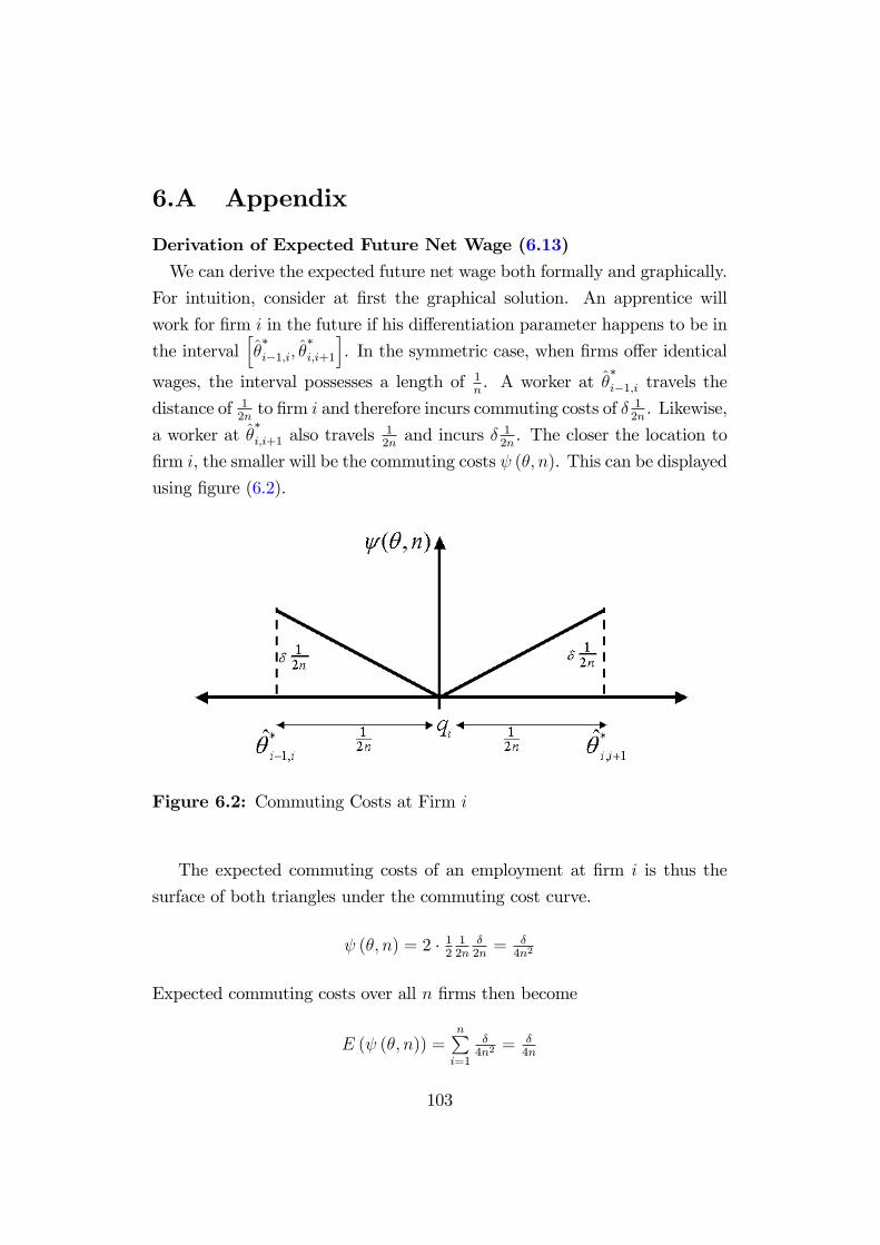
6.A Appendix

Derivation of Expected Future Net Wage (6.13)We can derive the expected future net wage both formally and graphically.

For intuition, consider at �rst the graphical solution. An apprentice will

work for �rm i in the future if his di¤erentiation parameter happens to be in

the intervalh��i�1;i; �

�i;i+1

i. In the symmetric case, when �rms o¤er identical

wages, the interval possesses a length of 1n. A worker at �

�i�1;i travels the

distance of 12nto �rm i and therefore incurs commuting costs of � 1

2n. Likewise,

a worker at ��i;i+1 also travels

12nand incurs � 1

2n. The closer the location to

�rm i, the smaller will be the commuting costs (�; n). This can be displayed

using �gure (6.2).

Figure 6.2: Commuting Costs at Firm i

The expected commuting costs of an employment at �rm i is thus the

surface of both triangles under the commuting cost curve.

(�; n) = 2 � 1212n

�2n= �

4n2

Expected commuting costs over all n �rms then become

E ( (�; n)) =nPi=1

�4n2

= �4n

103

Figure (6.3) illustrates this for the case of four �rms.

Figure 6.3: Commuting Costs for n = 4

Now consider the formal solution. A worker�s expected future net wage

can be displayed by the expected value of the future net wage. It derives

from the integral over � of the net wage ~w (�; n) weighted with the probability

function f (�).

E ( ~w�) =

Z 1

0

~w�(�; n)f (�) d�

Recall that a worker�s future net wage consists of the wage at the future

employer minus commuting costs, ~w�(�) = w�i � � jqi � �j. In the symmetriccase under consideration, �rms o¤er identical wages w�, but workers net wage

will result after commuting costs are taken into account. These costs depend

on a worker�s location and the number of �rms.

E ( ~w�) =

Z 1

0

(w� � n � (�; n)) f (�) d�

A worker would work for �rm i if her di¤erentiation parameter � lies in the

intervalh��i�1;i; �

�i;i+1

i, i.e. from being indi¤erent to work for �rm i � 1 and

to work for �rm i + 1. Expected commuting costs when working for �rm i

can be derived from the sum of two intervals

(�; n) = �

Z qi

��i�1;i

(qi � �) d� + �

Z ��i;i+1

qi

(� � qi) d�

104

Dissolving the integral obtains

(�; n) = ��qi� � 1

2�2�qi��i�1;i

+ ��12�2 � qi�

��i;i+1qi

which is

(�; n) = ��12q2i � qi�

�i�1;i +

12��2i�1;i

�+ �

�12��2i;i+1 � qi�

�i;i+1 +

12q2i

�This can be simpli�ed and rearranged to

(�; n) = ��q2i + �

�i�1;i

�12��i�1;i � qi

�+ �

�i;i+1

�12��i;i+1 � qi

��Now recall that �rms are considered to be distributed evenly across space.

Firm i�s location is simply qi = i�1n. Moreover, in the symmetric case, the

indi¤erent workers are located at ��i�1;i =

2i�32n

and ��i;i+1 =

2i�12n. From

inserting follows

(�; n) = ��

i�1n

�2+ 2i�3

2n

�122i�32n� i�1

n

�+ 2i�1

2n

�122i�12n� i�1

n

��Simplifying the fractions gives

(�; n) = ��

i�1n

�2+ 2i�3

2n

�2i�34n� 4i�4

4n

�+ 2i�1

2n

�2i�14n� 4i�4

4n

��or

(�; n) = ��

i�1n

�2 � 2i�32n

2i�14n� 2i�1

2n2i�34n

�which then reduces to

(�; n) = ��1n2

�i2 � 2i+ 1

�� 1

4n2

�4i2 � 8i+ 3

��or

(�; n) =�

4n2

Inserting (�; n) into the formula for the expected future net wage from

105

above then yields

E ( ~w�(�)) =

Z 1

0

�w� � n

�

4n2

�f (�) d�

Under the assumption of an uniform distribution, f (�) = 1,this simpli�es to

E ( ~w�(�)) = w� � �

4n

Inserting for the future equilibrium wage w� then yields

E ( ~w�(�)) = v � �

n� �

4n= v � 5

4

�

n

which is equation (6.13).

Derivation of Welfare Function (4.23)Recall that the net wage of a worker � at �rm i is given by �rm�s wage

minus the commuting costs.

~w�(�) = w�i � � jqi � �j

Firm i employs all workers in the intervalh��i�1;i; �

�i;i+1

i. Commuting costs

of all workers at �rm i are thus given by the sum

Z qi

��i�1;i

� (qi � �) d� +

Z ��i;i+1

qi

� (� � qi) d�

In the symmetric case, we can insert qi = i�1n, �

�i�1;i =

2i�12n� 1

n= 2i�3

2nand

��i;i+1 =

2i�12n

which then allows to dissolve the integrals and obtain �4n2. The

social costs of commuting in all n �rms are therefore �4n. Social welfare in

period t consists of �rms�pro�ts n �n2Nt and net wages

�w�t � �

4n

�Nt which is

simply

Wt =

�vt �

�

4n

�Nt

106

Summing over both periods and including training costsPci (Ait) then yields

W =Xt;t+1

�t�1�vt �

�

4n

�Nt �

Xi

ci (Ait)

which is equation (4.23).

107

Chapter 7

Reimbursement Clauses

Chapter 5 analyzed training levy schemes to internalize spillovers from ap-

prenticeship training. The analysis drew attention to substantial practical

di¢ culties of such instruments caused by informational and administrative

requirements. Moreover, it revealed adverse e¤ects that substantially reduce

the impact of this policy. In light of these problems, alternative policies are

sought that enhance welfare without the shortcomings of training subsidies

and levies.

Some authors suggest contractual agreements between �rms and work-

ers to internalize training spillovers (Alewell 1997, Alewell & Richter 2001,

e.g.) . They point to the observation of work contracts in the real world

where �rms frequently negotiate reimbursement clauses when providing pro-

fessional or continuous on-the-job training. Several empirical studies con�rm

the common use of such agreements.1 Typically, they oblige workers to a

compensation for received training when unilaterally terminating the work

contract. Similarly, contracts sometimes specify a mandatory work period at

the training �rm or restrict the worker in another way beyond the training

period. For this reason, reimbursement clauses are often considered to reduce

1Note that unlike wages, which regularly enter social security or income tax statistics,reimbursement clauses are usually not statistically reported. Empirical evidence derivesmostly from case studies or surveys. Although surveys that have been conducted forGermany vary strongly in study design and poll size, they generally support the commonusage of reimbursement clauses. See Alewell (1997), 149¤., for an overview of severalstudies.

108

turnover of trained workers and thereby prevent training spillovers to arise

onto other �rms.

There are legal restrictions on such agreements. In particular, common

law, labor protection law, and case law prohibit �exploitative�clauses in work

contracts. While this generally applies for work contracts, the law speci�-

cally rules out reimbursement clauses in vocational training contracts. This

regulation has been questioned strongly. Alewell & Richter (2001) argue that

�rms have a natural interest to negotiate reimbursement clauses. By means

of such agreements, �rms intend to limit worker turnover and secure their

human capital investment against the risk of future quits. The ban on such

contractual agreements yet prohibits this instrument and thereby prevents

to address poaching and positive training spillovers. The authors therefore

conclude this regulation to be counterintentional since abolishing it could

help to internalize spillovers and increase apprenticeship training as well as

social welfare.

In view of the ongoing debate on vocational training policy, it is of course

an important question whether or not this claim is correct. Obviously, abol-

ishing a counterproductive regulation would be costless and therefore prefer-

able to introducing additional training incentives that necessarily bring along

further bureaucracy and distortions. Yet, surprisingly, there is little research

on reimbursement clauses or similar contractual arrangements. While several

legal contributions deal with the legitimacy of training clauses for professional

and continuous training, economic research on their private and social e¤ects

is scarce.

This chapter aims to provide an economic analysis of reimbursement

clauses in the context of frictional labor markets. It will extend the model

framework from previous chapters and incorporate conditional reimburse-

ment obligations. This shall �rstly allow to study their e¤ects on training,

wages and social welfare. Secondly, it shall allow for an appraisal of the reg-

ulation under question. Beforehand, however, legal conditions and existing

research on reimbursement obligations in training contracts will be reviewed.

109

7.1 Legal Terms and Conditions

Firms investing into on-the-job training inevitably face the risk of workers

quitting after the training period. They therefore seek to secure their human

capital investment by formulating training contracts that constitute claims in

the event of workers leaving after training. The general freedom of contract

entitles private parties to negotiate all terms and conditions of an employ-

ment contract. Accordingly, they may write a contract at their own will

that speci�es how to share costs, bene�ts, and risks of on-the-job training. A

reimbursement clause entitles the training �rm to claim a monetary compen-

sation in the event of the worker terminating the employment contract within

a certain period. Similarly, parties may agree on a mandatory work period

at the training �rm or specify other limitations on the worker to recompense

for training.

Obviously, any contractual arrangement is only valuable if claims can be

substantiated, exercised, and, if necessary, also enforced before a court of law.

Even if the apprentice were fully solvent when quitting and the reimburse-

ment amount could be collected, some agreements are void and unenforceable

due to common law, labor protection law, and case law. An extensive legal

literature investigates the admissibility of reimbursement clauses and similar

contractual provisions. It reviews both court decisions and legal practice of

speci�c training clauses and particular training programs (Becker-Scha¤ner

1991, Hanau & Sto¤els 1992, Alewell 1997, e.g.) .

For the purposes of this work it su¢ ces to outline the legal framework of

reimbursement clauses. As a simple legal yardstick, an agreement is admis-

sible as long as it balances the property right of the training �rm with the

employee�s right to freely choose her employment. However, the agreement

must not be excessive, prohibitive, and undue. Roughly speaking, it must

decrease over time and usually cannot exceed three years after completion of

the training (Alewell 1997, 154¤.).

Hanau & Sto¤els (1992) provide a legal summary, whereby the admissi-

bility of any training clause can be determined from three criteria.

110

1. Is the clause admissible on its merits?

This criterion demands a legitimate and approvable interest of the em-

ployer to use this clause. Furthermore it requires the clause to be

reasonable and acceptable for the employee.

2. Is the form of the clause admissible?

This criterion addresses particular terms of the training clause. Is the

time span tolerable? Is the amount to reimburse or an equivalent re-

striction tolerable? Is the condition which creates the reimbursement

obligation tolerable?

3. Is the employer acting unduly when exercising the claim?

This criterion excludes unfair practices that are not with the legal prin-

ciple of good faith.

Within these legal restraints, reimbursement clauses substantiate enforce-

able claims in work contracts. By contrast, they are null and void in vo-

cational training contracts. The federal law on vocational training speci�-

cally rules out any arrangement that limits an apprentice in her occupational

choice.2 This regulation is commonly justi�ed by a need of protecting appren-

tices from being exploited by the training �rm. It is argued that apprentices

typically possess little bargaining power since they are young and inexperi-

enced labor market entrants that require a vocational quali�cation.

In summary, reimbursement clauses are admissible in normal employment

contracts if training is mostly general. For vocational training, however, they

are prohibited by law. To be able to evaluate this legal framework we will

now turn to the economics of reimbursement clauses.

2This ban follows from §5 BBiG. See the appendix for the precise text of the law.

111

7.2 Previous Research

Unlike the legal literature, economic research on reimbursement clauses is

scarce. In business economics, such agreements are discussed within hu-

man resources management. This literature emphasizes training contracts

as managerial tools to bind workers to the �rm and secure training invest-

ments (Sadowski 2002, 60f.). Human capital theory, by contrast, pays little

attention to reimbursement clauses. In particular, it lacks an analysis on the

e¤ects of such agreements on worker turnover, wages, training provision and

spillovers. In order to provide a starting point for our analysis, this section

reviews human capital theory with respect to reimbursement clauses.

7.2.1 ReimbursementClauses inPerfect LaborMarkets

Classical human capital theory has not explicitly studied on-the-job training

with reimbursement clauses. Nevertheless, such agreements can be analyzed

in this theoretical setting. To do so, again assume perfectly competitive labor

markets and distinguish general and �rm-speci�c training.3

Human capital theory predicts �rms not to pay for general training as

it brings along a congruent wage increase that inhibits the training �rm to

collect any compensation for its training e¤orts. If the �rm nevertheless

provides this training, the worker will bear the investment costs in form of a

wage cut in the training period or through a training loan. Since the worker

receives all returns and incurs all costs, training provision will be e¢ cient

and independent of worker turnover. As the worker is paying for the training

in any case, there is no economic need for a contractual agreement contingent

upon resignation. By consequence, a reimbursement clause does not a¤ect

the training decision.

Firm-speci�c training, by contrast, is valuable only within the training

�rm. It leaves workers�outside wages una¤ected and all returns of this type

of training accrue to the training �rm. Should the worker quit, however,3For an extended presentation of human capital investments in perfect labor markets

see above in section 3.2.

112

the investment vanishes. Firms will therefore try to decrease turnover by

o¤ering a training contract with appropriate incentives. Such a contract

makes the trainee a co-investor by sharing costs and returns of the �rm-

speci�c investment. But this cannot be achieved through a reimbursement

clause. It rather characterizes a barrier to quit than a sharing device since it

puts a unilateral burden on the worker in case of contract termination.

To summarize, standard human capital theory negates a need for reim-

bursement clauses. It predicts that both general and �rm-speci�c on-the-job

training is e¢ cient without any reimbursement obligation on workers when

quitting the �rm. From this follows, however, that the theory can neither

explain the existence nor the use of such contractual arrangements. This im-

plication of standard human capital theory for reimbursement clauses is at

odds with empirical observation, practical experience as well as common in-

tuition. As training clauses with conditional reimbursement are widespread,

a revised theory is therefore required.

7.2.2 ReimbursementClauses in Imperfect LaborMarkets

Alewell (1997) takes up this contradiction in the context of continuous on-

the-job training. Starting from the observation that �rms often provide this

training using reimbursement obligations, she proposes a simple model of

human capital investment under uncertainty. We will brie�y discuss her

approach and thereby provide a starting point and reference for our own

analysis.4

Her exposition starts from the assumption that �rms incur costs and

receive returns from providing continuous training. Let x be the amount of

training chosen and c(x) denote the present value of monetary training costs.

Similarly, the present value of training returns is represented by a function

v(x). As is common throughout the literature, she assumes a convex cost

4For uniformity and ease of reading, the subsequent review continues in our notation.See Alewell (1997), 160¤., for the original presentation.

113

function, c0 > 0 and c00 � 0, but decreasing marginal returns to the volumeof training, v0 > 0 and v00 < 0.5

When providing continuous training, the �rm faces uncertainty. First,

there is the risk of uncertain investment returns. This is the investment risk.

Second, there is the risk of workers quitting the �rm after training. This

is commonly referred to as turnover risk. In order to model this, Alewell

proposes two separate two-point distributions. With probability p training

yields high returns vh(x); and with the complementary probability 1 � p it

yields low returns vn(x). Similarly, she assumes workers to quit the �rm with

probability q and stay with probability 1� q.

Given this set-up, �rms�optimal training investment can be derived and

compared to the benchmark of a benevolent social planner. In line with

human capital theory, Alewell �rst discusses general and then �rm-speci�c

training.

General TrainingSince general training is socially valuable whether or not the worker re-

mains with the training �rm, a benevolent social planner would maximize

the expected returns from training minus the training costs.

argmaxfxg

�pvh (x) + (1� p) vn (x)� c(x)

In the social optimum, therefore, training is to be carried out such that the

expected marginal returns equal the marginal training costs. This follows

straightforward from the �rst order condition.

pvh0 + (1� p) vn0 = c0

With this reference in mind, now consider the decision problem of a pro�t-

5Alewell also considers e¤ects of continuous training on workers� utility levels. Shemodels this by postulating non-monetary e¤ects that can either be costs, such as workers�costs associated with time and e¤ort spent on training, or bene�ts, such as utility fromlearning and experience. However, the qualitative results of her model do not depend onnon-monetary e¤ects incurred by workers. In order to shorten and simplify the exposition,they are therefore neglected here.

114

maximizing �rm.

argmaxfxg

�(1� q)

�pvh (x) + (1� p) vn (x)

�� c(x)

Because trained workers quit with probability q, �rm�s training returns are

only the expected return weighted by the probability of the worker staying

with the �rm. Clearly, there is an externality as some returns are lost to the

training �rm, but not to society. The private optimum can be represented

by the following �rst order condition.

pvh0 + (1� p) vn0 =1

1� qc0

It states that the expected marginal returns are to equal the marginal costs

weighted by the inverse of the remainder probability. Since 1 � q < 1, the

right hand side will be larger than before. Thus, in comparison to the social

optimum, there will be underinvestment in continuous training.

Now introduce a reimbursement clause whereby the training �rm can

claim some compensation for training in case the worker quits. Denote the

repayment amount by a positive and increasing function b(x). This formu-

lation allows the repayment to depend on the amount of training received.

Firm�s optimization problem thereby alters to

argmaxfxg

�(1� q)

�pvh (x) + (1� p) vn (x)

�+ qb (x)� c (x)

which results into the following �rst order condition

(1� q)�pvh0 + (1� p) vn0

�+ qb0 = c0

With q > 0 and b0 > 0, a conditional repayment obligation increases train-

ing incentives. Thus, a reimbursement clause can possibly internalize the

external e¤ect. In this simple setting, in fact, an appropriate choice of the

reimbursement amount can perfectly internalize the external e¤ect and fully

restore e¢ cient training. In order to demonstrate this, either set the condi-

115

tional repayment obligation equal to training costs, b (x) = c (x). Likewise,

the repayment could be set equivalent to �rm�s expected net training return,

b (x) = pvh (x) + (1� p) vn (x) � c (x). In both cases, the �rst order con-

ditions then shows �rm�s individual training decision to be identical to the

social choice.6

In view of this analysis, Alewell concludes that reimbursement clauses

can reduce the externality problem of general on-the-job training. For voca-

tional training, she therefore recommends to abolish the present regulation

and to permit to negotiate conditional repayment obligations within training

contracts.

Speci�c TrainingWe now follow Alewell in also investigating reimbursement clauses in the

context of speci�c training. Since this type of training only yields returns

when working with the training �rm, socially optimal training follows from

argmaxfxg

�(1� q)

�pvh (x) + (1� p) vn (x)

�� c (x)

The �rst-order condition states that training is e¢ cient when expected mar-

ginal returns weighted by the remainder probability are equal to marginal

training costs. As �rm-speci�c training has no value to other �rms, there are

no spillovers and training is e¢ cient.

(1� q)�pvh0 + (1� p) vn0

�= c0

Although all returns of �rm-speci�c training accrue to the �rm, it will be

reluctant to incur training costs. For if the work contract is terminated, the

investment is lost. This can be mitigated by sharing the training investment

so that both parties will be hurt from contract separation.

To demonstrate a shared investment, let " denote worker�s share of train-

6In an extended analysis, Alewell also discusses cases where over- or underprovisioncould arise with reimbursement clauses when turnover risk and investment risk are inter-related.

116

ing returns where 0 � " � 1. Similarly, let worker�s share of training costs

be �, 0 � � � 1. In order for the worker to participate in �rm-speci�c train-ing, the training contract must satisfy the worker�s participation constraint

(1� q) "�pvh0 + (1� p) vn0

�� c (x) � 0. Firm�s investment problem can

thus be stated by

argmaxfxg

�(1� q) (1� ")

�pvh0 + (1� p) vn0

�� (1� �) c (x)

s.t. (PC)

As the �rst order condition yields the same equation as before, training with

the sharing rule remains e¢ cient.

(1� q)�pvh0 + (1� p) vn0

�= c0

Alewell points out that �rms could just as well use a reimbursement clause

to share the �rm-speci�c investment. To show this, let the worker as before

receive a share " of training returns when with the �rm, but repay an amount

b(x) when quitting. With this speci�cation, worker�s participation constraint

is now (1� q) "v (x)� qb (x) � 0. From �rm�s modi�ed decision problem

argmaxfxg

�(1� q) (1� ")

�pvh0 + (1� p) vn0

�� c (x) + qb (x)

s.t. (PC)

then directly follows the optimality condition

(1� q)�pvh0 + (1� p) vn0

�= c0

This is the same equation as above. Reimbursement clauses are therefore a

possible contractual means to share costs and returns of training among both

parties. Yet, according to this model, a training contract with cost sharing

or reimbursement clauses are essentially equivalent. Thus, a statement on

when either instrument is preferred cannot be inferred.

Heterogeneous Workers and Asymmetric InformationReimbursement clauses may additionally possess screening properties. If

workers di¤er in their quitting probability, but this information is unavailable

117

to �rms, then reimbursement clauses can be used as a self-selection device

to distinguish between heterogeneous workers. Alewell demonstrates this

property by assuming two types of workers. The high type has a quitting

probability qh while the low type has a quitting probability ql, with qh >

ql. Type information is asymmetrically distributed, i.e. workers know their

quitting probability, but �rms possess only general information on turnover

and therefore cannot distinguish between worker types.

Since speci�c training is lost in case of termination, a �rm would naturally

like to train the low type only. To this end, it could o¤er a menu of training

contracts in such a way that the low type accepts, while the high type rejects,

i.e. only the participation constraint of the low type is ful�lled.

�1� qh

�"E [v (x)]� qhb (x) < 0�

1� ql�"E [v (x)]� qlb (x) � 0

Straightforward rearrangements allow to summarize this menu of contracts

in a self-selection condition.

ql � "E [v (x)]

b (x) + "E [v (x)]< qh

By setting b (x) and " in an appropriate way, the employer can ensure that

only the low type will accept the o¤er.

If only the low type accepts the training contract, then lower turnover

results into higher training returns. Given the optimal training condition�1� ql

�E [v0 (x)] = c0 and ql < qh, this implies the �rm to o¤er a higher

level of �rm-speci�c training.

Despite the advantages of screening to reduce turnover risk, practical con-

cerns impose serious objections. Typically, workers with a lower propensity

to quit are older, less mobile, or in lack of job alternatives. From a long term

business perspective, therefore, it seems risky to concentrate �rm-speci�c

training on workers with such characteristics (Alewell 1997, 174).

118

7.2.3 Discussion

This literature review points out that conventional human capital theory can-

not explain training contracts to include reimbursement clauses. Clearly, this

prediction is troubling as it runs counter to empirical surveys and common

experience. Alewell�s model of continuous on-the-job training addresses this

contradiction and aims to explain their use in training contracts. According

to her analysis, worker turnover deteriorates on-the-job training. In case of

general training, it causes a training externality that leads to an underpro-

vision of training. Here, a reimbursement clause denotes a simple contrac-

tual instrument to internalize the external e¤ect and thereby restore e¢ cient

training incentives. In case of speci�c training, no externality arises as all

costs and returns accrue to the training parties. Still, reimbursement clauses

could enter training contracts within a mechanism to share the training in-

vestment. Moreover, if worker turnover di¤ers and �rms face asymmetric

information, then reimbursement clauses could act as a self-selection device.

This could allow to di¤erentiate among heterogeneous workers and increase

the �rm-speci�c investment.

On the basis of her analysis, Alewell concludes that reimbursement clauses

can enhance e¢ ciency as they internalize spillovers or reduce information

asymmetries. Hence, legal restrictions on such contractual terms should be

lifted. However, some conclusions arise from simplifying assumptions in the

analysis. They now demand further discussion.

Alewell�s approach essentially models continuous on-the-job training as an

investment problem under uncertainty. In this setting, a representative �rm

decides on continuous training subject to uncertain returns and the risk of

workers leaving the �rm. Training costs, investment returns and turnover risk

are exogenously given and independent of labor market conditions. While the

set-up has the advantage of being simple, it has the drawback of neglecting

the labor market. Unfortunately, this is not an innocuous simpli�cation of the

problem as the labor market provides an important channel for human capital

investments. This was also stressed by Becker (1962) who observed that

market wages determine �rms�and workers�returns to on-the-job training

119

and likewise a¤ect turnover. Even though some quits might be driven by

exogenous forces, worker turnover clearly results from di¤erences between

the wage of the �rm and its close competitors. Assuming turnover risk to be

solely exogenous is therefore questionable. Moreover, since worker turnover

in this model causes training spillovers, the policy conclusion critically hinges

on this assumption, too.

In sum, Alewell provides a �rst comprehensive analysis of reimbursement

clauses, but the results draw from quite restrictive assumptions. This calls for

a revised approach that relaxes the assumptions and checks whether the re-

sults can be maintained. In particular, an improved analysis requires a model

with endogenous wage setting and endogenous worker turnover which re�ects

wages to be the central mechanism for on-the-job training and turnover. Our

simple training model allows for this. In the next section we therefore extend

the model and study reimbursement clauses.

120

7.3 SimpleModel with Reimbursement Clauses

Return to the simple model of chapter 4. As before, we distinguish two peri-

ods, a training period where on-the-job training of apprentices occurs, and a

poaching period where workers can leave for other employers. Now addition-

ally, the training contract may entail a reimbursement clause. We model this

clause in form of an absolute payment bi that �rm i can claim in case the

worker quits after training.7 Clearly, when choosing among competing wage

o¤ers in the poaching period, workers will take this monetary obligation into

account.

With this slight modi�cation, now again solve the game using backward

induction, i.e. by �rst analyzing the poaching period and then turning to the

training period. Figure (7.1) summarizes the time structure of the extended

model.

Figure 7.1: Model Time Structure with Reimbursement Clauses


In the poaching period, �rms post wage o¤ers to compete for three groups

of workers: apprentices trained at �rm 1, apprentices trained at �rm 2 and

existing skilled workers. Wage o¤ers may be set separately for each group,

7In this setting, in contrast to Alewell�s model where training intensity can be chosen,�rms decide only about the number of workers to train. An absolute reimbursementamount therefore su¢ ces.

121

wiA1, wiA2 and wiL. This just re�ects the common practice to di¤erentiate

on applicants�information through a curriculum vitae or interviews.8

A repayment obligation a¤ects the apprentices�choice between alterna-

tive employers. Some apprentices will remain with the training �rm while

others will choose to reimburse and quit for �rm 2. In our model, the in-

dividual decision depends on wage o¤ers, personal characteristics, and the

reimbursement amount. An arbitrage consideration can again be used to

determine the decisive worker in each group who is indi¤erent to work for

either �rm. As before, workers are assumed to be uniformly distributed along

a Hotelling street and to incur frictional costs to work for either �rm. Thus,

when deciding whether to stay or quit, workers compare the net wage when

staying with the training �rm to the net wage of another employer less the

reimbursement amount bi.

For skilled workers L, the arbitrage condition is identical to above

w1L � ��L = w2L � ��1� �L

�(7.1)

Firms�share of this workforce then again follow from �L =w1L�w2L+�

2�and

1� �L =w2L�w1L+�

2�. Next consider apprentices trained by �rm 1. Here it is

the apprentice with characteristics �A1 who is indi¤erent between the wage

o¤er of �rm 1 or leaving for �rm 2 and reimbursing b1.

w1A1 � ��A1 = w2A1 � ��1� �A1

�� b1 (7.2)

Thus, �A1 is the fraction of apprentices trained by �rm 1 that remains while

a fraction 1� �A1 quits for the competitor.

�A1 =w1A1 � w2A1 + � + b1

2�

1� �A1 =w2A1 � w1A1 + � � b1

2�

Prima facie, an obligation to compensate the �rm for training when quit-

8Note that separate wage o¤ers did not matter before as worker groups did not di¤er.With the repayment obligation, however, they do.

122

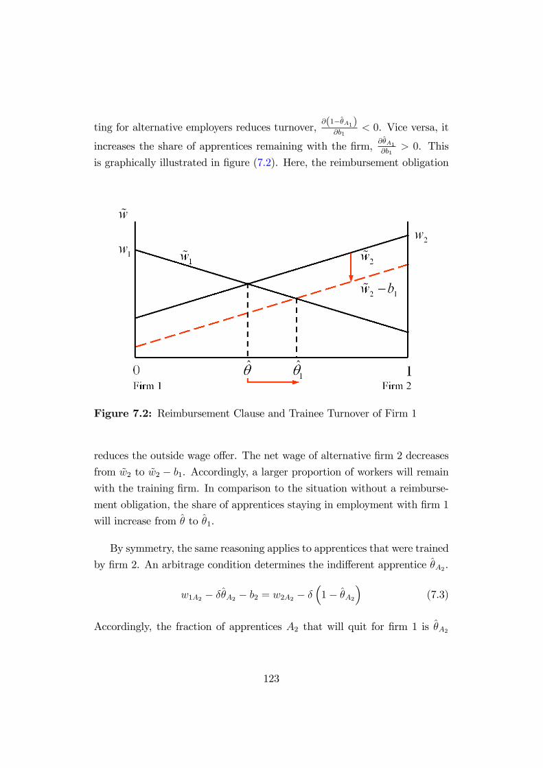
ting for alternative employers reduces turnover,@(1��A1)

@b1< 0. Vice versa, it

increases the share of apprentices remaining with the �rm, @�A1@b1

> 0. This

is graphically illustrated in �gure (7.2). Here, the reimbursement obligation

Figure 7.2: Reimbursement Clause and Trainee Turnover of Firm 1

reduces the outside wage o¤er. The net wage of alternative �rm 2 decreases

from ~w2 to ~w2 � b1. Accordingly, a larger proportion of workers will remain

with the training �rm. In comparison to the situation without a reimburse-

ment obligation, the share of apprentices staying in employment with �rm 1

will increase from � to �1.

By symmetry, the same reasoning applies to apprentices that were trained

by �rm 2. An arbitrage condition determines the indi¤erent apprentice �A2.

w1A2 � ��A2 � b2 = w2A2 � ��1� �A2

�(7.3)

Accordingly, the fraction of apprentices A2 that will quit for �rm 1 is �A2

123

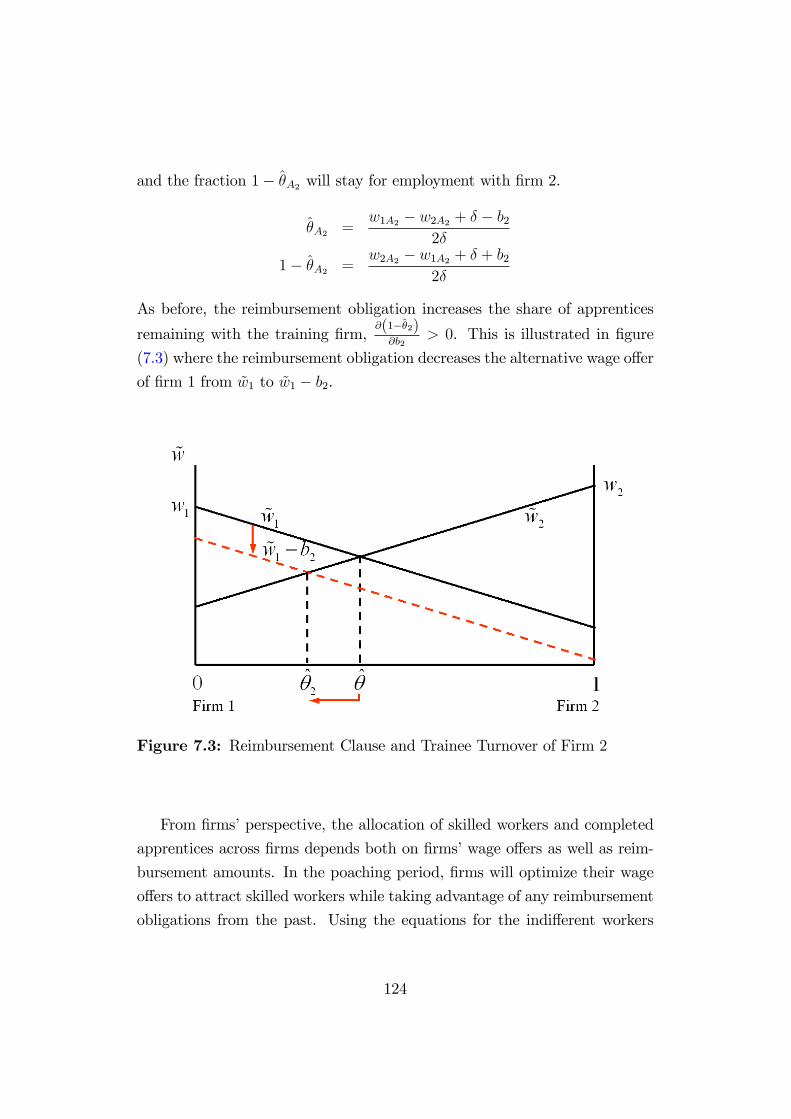
and the fraction 1� �A2 will stay for employment with �rm 2.

�A2 =w1A2 � w2A2 + � � b2

2�

1� �A2 =w2A2 � w1A2 + � + b2

2�

As before, the reimbursement obligation increases the share of apprentices

remaining with the training �rm,@(1��2)@b2

> 0. This is illustrated in �gure

(7.3) where the reimbursement obligation decreases the alternative wage o¤er

of �rm 1 from ~w1 to ~w1 � b2.

Figure 7.3: Reimbursement Clause and Trainee Turnover of Firm 2

From �rms�perspective, the allocation of skilled workers and completed

apprentices across �rms depends both on �rms�wage o¤ers as well as reim-

bursement amounts. In the poaching period, �rms will optimize their wage

o¤ers to attract skilled workers while taking advantage of any reimbursement

obligations from the past. Using the equations for the indi¤erent workers

124

�k (:) from above, �rm�s pro�t functions are given by (7.4) and (7.5).

maxfw1L;w1A1;w1A2g

�1 =X

k=A1;A2;L

(v1 � w1k) �k (:) k +�1� �A1 (:)

�b1A1 (7.4)

maxfw2L;w2A1;w2A2g

�2 =X

k=A1;A2;L

(v2 � w2k)�1� �k (:)

�k + �A2 (:) b2A2 (7.5)

In contrast to before, the pro�t functions now consist of two terms. The �rst

term represents the margin of productivity over wages when employing skilled

workers. The second term denotes repayment revenues from apprentices

quitting for another employer.

Again, obtain the Hotelling-Nash-equilibrium from the intersection of

�rms� pro�t-maximizing wage reaction functions. See the appendix for a

detailed derivation. The equilibrium wages for workers

w�1L =2

3v1 +

1

3v2 � �

w�2L =1

3v1 +

2

3v2 � �

Note that they are identical to before. For apprentices trained by �rm 1,

however, equilibrium wage o¤ers are

w�1A1 =2

3v1 +

1

3v2 � � � b1

w�2A1 =1

3v1 +

2

3v2 � �

and for apprentices trained by �rm 2

w�1A2 =2

3v1 +

1

3v2 � �

w�2A2 =1

3v1 +

2

3v2 � � � b2

In view of these equilibrium wage o¤ers, we can state the next proposition.

Proposition 22 An obligation to reimburse for training conditional uponquitting leads to a loss for the worker regardless of remaining at or quitting

125

from the �rm.

Proof. For i = f1; 2g, @w�Ai

@bi= �1.

To understand this result, simply observe that a reimbursement obligation

introduces additional switching costs for the worker. It o¤ers �rms further

monopsony power on apprentices and thereby allows to decrease the wage

for continued employment by this amount. Thus, if remaining with the �rm,

apprentices forgo a higher wage. If quitting, they earn the higher competing

wage, but have to reimburse for training through a nominal transfer.

As before, use the equilibrium wages to determine worker allocation. The

allocation of skilled workers that have no reimbursement obligation will be

identical to before.

��L =

w�1L � w�2L + �

2�=1

2+v1 � v26�

1� ��L =

w�2L � w�1L + �

2�=1

2� v1 � v2

6�

However, the same allocation also results for apprentices trained by �rm 1

��A1

=w�1A1 � w�2A1 + � + b1

2�=1

2+v1 � v26�

1� ��A1

=w�2A1 � w�1A1 + � � b1

2�=1

2� v1 � v2

6�

as well as for apprentices trained by �rm 2.

��A2

=w�1A2 � w�2A2 + � � b2

2�=1

2+v1 � v26�

1� ��A2

=w�2A2 � w�1A2 + � + b2

2�=1

2� v1 � v2

6�

This is summarized in the next proposition:

Proposition 23 A reimbursement obligation does not a¤ect turnover.

Proof. For k = fA1; A2; Lg, clearly @��k

@bk= 0.

126

Contrary to expectations and in opposition to Alewell�s result, a repay-

ment obligation does not a¤ect worker turnover. This prediction follows

directly from the previous proposition. Since a reimbursement clause has

workers repay for training regardless of whether or not she quits, equilibrium

turnover remains una¤ected. The equilibrium worker allocation depends only

on �rm productivity, personal characteristics and frictions.

Insert equilibrium wages and worker allocations into �rms�pro�t func-

tions (7.4) and (7.5) and obtain �rms�equilibrium pro�ts.

��1 =(v1 � v2 + 3�)

2

18�(A1 + A2 + L) + b1A1

��2 =(v2 � v1 + 3�)

2

18�(A1 + A2 + L) + b2A2

Note, that a reimbursement clause increases �rms�pro�ts when apprentices

have been trained by the �rm. This follows immediately from @��i@bi

> 0, for

Ai > 0. Put di¤erently, a reimbursement clause gives additional returns to

the �rm in the poaching period. We will now investigate, how this a¤ects

the training decision.


Given the results from the poaching period, now turn to the training period

where �rms can decide on the number of apprentices, trainee wages and the

reimbursement amount. Moreover, for apprentices to enter into training, the

�rm must respect the participation constraint.

Training Participation without Credit ConstraintsIf capital markets are perfect and allow for transfer of funds between both

periods, an unskilled worker will accept the training contract if �in present

value terms � the net income from training exceeds the net income from

remaining unskilled. From the participation constraint (4.6) follows that with

unskilled wages normalized to zero and in absence of any credit constraints,

127

the unskilled worker will be willing to forego earnings in the training period

at most equal to the discounted expected future net income, �wai � �Ei ( ~w).

Using the equilibrium wages from the poaching period, the participation

constraints are

� wa1 � �E1 ( ~w) = ��12(v1 + v2) +

136�(v1 � v2)

2 � 54� � b1

�(7.6)

�wa2 � �E2 ( ~w) = ��12(v1 + v2) +

136�(v1 � v2)

2 � 54� � b2

�(7.7)

See again the appendix for a complete derivation of the expected net wages.

Note that the participation constraint di¤ers to the simple model only by the

reimbursement amount bi. Firms�training decision problem follows from

argmaxfA1;wa1 ;b1g

f��1 � wa1A1 � c1(A1)g s.t. (PC1)

argmaxfA2wa2 ;b2g

f��2 � wa2A2 � c2(A2)g s.t. (PC2)

If �rms possess all bargaining power, the participation constraint will be

binding and can be substituted into each �rm�s decision problem. Replacing

for ��1 and ��2 as well as w

a1 and w

a2 , the �rst order conditions are

��12(v1 + v2) +

112�(v1 � v2) (v1 � v2 + 4�)� 3

4��= c01 (7.8)

��12(v1 + v2) +

112�(v2 � v1) (v2 � v1 + 4�)� 3

4��= c02 (7.9)

Proposition 24 In absence of credit constraints, reimbursement clauses leavetraining e¢ ciency unaltered.

Proof. For i = f1; 2g, @Ai@bi= 0.

A reimbursement clause does not enter the optimality conditions for train-

ing. The intuition for this result is as follows: The repayment obligation re-

duces worker�s future income regardless of whether or not she remains with

the �rm. With a binding participation constraint, worker�s training incen-

tives are reduced. With the reimbursement clause, by contrast, future pro�ts

of the training �rm increase by the same amount. As both e¤ects cancel out,

128

total incentives for training are unaltered. The reimbursement clause just

shifts worker�s cost burden from the trainee wage to the foregone future

wage.

Training Participation with Credit ConstraintsNow study the private training condition under credit constraints. With

the credit constraint (4.7) binding, wai = m, the apprentice is restrained

from foregoing earnings necessary for to �rm to provide e¢ cient training. As

she cannot borrow up to her discounted future net income, we have m >

��Ei ( ~w). Firms�training decision problem thus alters

argmaxfA1;wa1 ;b1g

f��1 � wa1A1 � c1(A1)g s.t. (PC1) and (CC)

argmaxfA2wa2 ;b2g

f��2 � wa2A2 � c2(A2)g s.t. (PC2) and (CC)

Replacing for ��1 and ��2 as well as w

a1 and w

a2 , the �rst order conditions are

��(v1�v2+3�)2

18�+ b1

��m = c01 (7.10)

��(v2�v1+3�)2

18�+ b2

��m = c02 (7.11)

The bracket term denotes �rm�s pro�ts from an additional apprentices whereas

�m denotes the worker�s constrained investment.9 At the constrained op-

timum, both should be equal to the marginal costs. Since �rms�optimal

training now depends on the reimbursement amount bi, we can state the

following proposition.

Proposition 25 Reimbursement clauses constitute an implicit �rm-providedtraining loan since they defer a worker�s training investment to the future.

If workers face credit constraints, then this can reduce the ine¢ ciency and

increase on-the-job training.

Proof. For i = f1; 2g and m > ��Ei ( ~w), @Ai@bi> 0.

9Note that the credit constraint is a negative amount, i.e. the amount that the appren-tice could borrow.

129

In order to explain this result, observe that credit constraints inhibit ap-

prentices from su¢ ciently foregoing earnings or taking up adequate training

loans. This would normally give rise to an underinvestment in general train-

ing. However, by means of a contractual obligation to reimburse, apprentices

can (fully or partially) defer their training investment to the future. Either

they reimburse the �rm for training when quitting or they pay through fore-

gone wages. By consequence, a reimbursement clause can be characterized

as an implicit training loan. As it can mitigate investment-restraining credit

constraints, the use of this instrument enhances e¢ ciency.

130

7.4 Generalized Model with Reimbursement

Clauses

We will now extend the analysis to a labor market with an inde�nite number

of �rms. This allows, as before, to generalize the simple two-�rm setting and

to compare results of competitive labor markets with many �rms to rather

incompetitive labor markets with only few �rms.

Return to the model of chapter 6 and again consider a Salop-circle of

unit length with n �rms evenly located across the circular economic space.

In addition, worker and training �rm can now agree to sign a training contract

obliging the worker to reimburse for training when leaving the �rm in the

future.


In the poaching period, after having completed the apprenticeship, appren-

tices choose among �rms�wage o¤ers. They will work for the �rm o¤ering the

highest net income, i.e. the highest wage net of frictional costs and training

reimbursements. Let bi again denote the repayment amount when quitting

from training �rm i. Thus, the net wage ~wj of a worker with characteristics

�, trained at �rm i and working for �rm j can now be written as

~wj (�) =

�wj � � jqj � �j if j = i

wj � � jqj � �j � bi if j 6= i

�(7.12)

Consider apprentices with characteristics in the interval [qi; qi+1]. They will

arbitrage between the wage o¤ers of �rm i and �rm i + 1. Let �i;i+1 be

the worker who is indi¤erent between working for either �rm. Net wages of

working at either �rm are equal for this worker and the indi¤erence condition

(7.13) is ful�lled.

wi � ��i;i+1 � qi

�= wi+1 � �

�qi+1 � �i;i+1

�� bi (7.13)

131

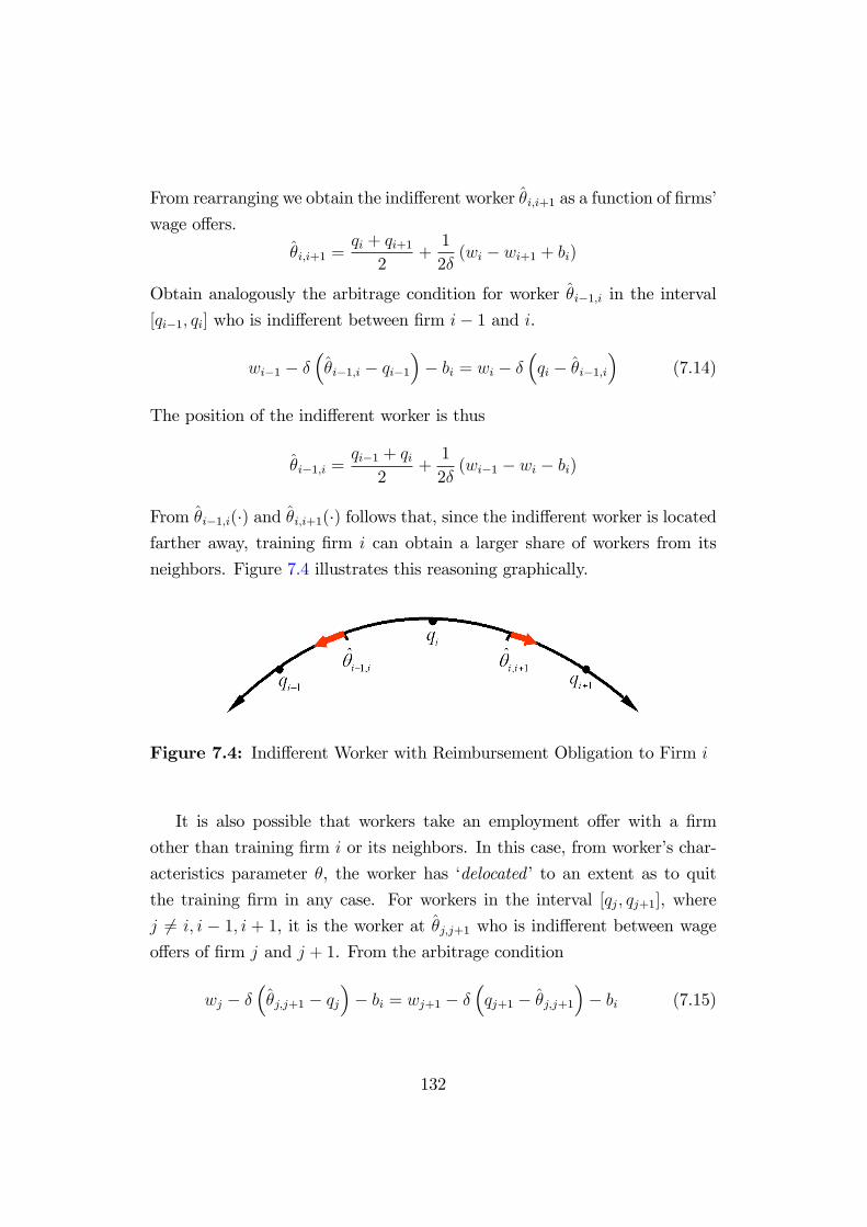
From rearranging we obtain the indi¤erent worker �i;i+1 as a function of �rms�

wage o¤ers.

�i;i+1 =qi + qi+1

2+1

2�(wi � wi+1 + bi)

Obtain analogously the arbitrage condition for worker �i�1;i in the interval

[qi�1; qi] who is indi¤erent between �rm i� 1 and i.

wi�1 � ��i�1;i � qi�1

�� bi = wi � �

�qi � �i�1;i

�(7.14)

The position of the indi¤erent worker is thus

�i�1;i =qi�1 + qi

2+1

2�(wi�1 � wi � bi)

From �i�1;i(�) and �i;i+1(�) follows that, since the indi¤erent worker is locatedfarther away, training �rm i can obtain a larger share of workers from its

neighbors. Figure 7.4 illustrates this reasoning graphically.

Figure 7.4: Indi¤erent Worker with Reimbursement Obligation to Firm i

It is also possible that workers take an employment o¤er with a �rm

other than training �rm i or its neighbors. In this case, from worker�s char-

acteristics parameter �, the worker has �delocated�to an extent as to quit

the training �rm in any case. For workers in the interval [qj; qj+1], where

j 6= i; i � 1; i + 1, it is the worker at �j;j+1 who is indi¤erent between wageo¤ers of �rm j and j + 1. From the arbitrage condition

wj � ��j;j+1 � qj

�� bi = wj+1 � �

�qj+1 � �j;j+1

�� bi (7.15)

132

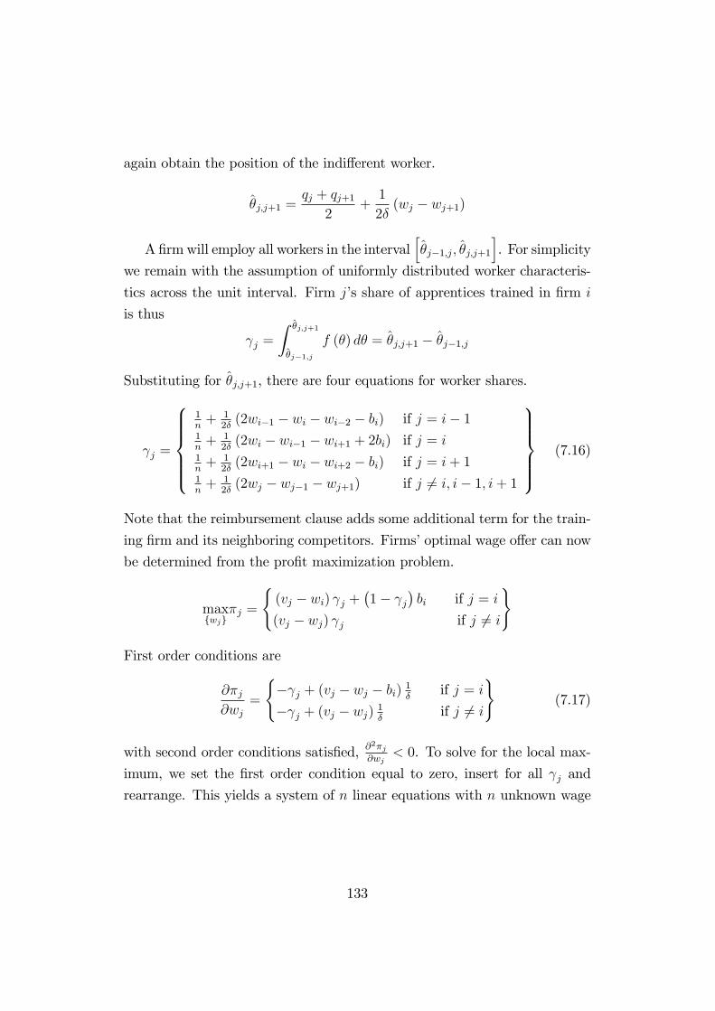
again obtain the position of the indi¤erent worker.

�j;j+1 =qj + qj+1

2+1

2�(wj � wj+1)

A�rmwill employ all workers in the intervalh�j�1;j; �j;j+1

i. For simplicity

we remain with the assumption of uniformly distributed worker characteris-

tics across the unit interval. Firm j�s share of apprentices trained in �rm i

is thus

j =

Z �j;j+1

�j�1;j

f (�) d� = �j;j+1 � �j�1;j

Substituting for �j;j+1, there are four equations for worker shares.

j =

8>>>><>>>>:1n+ 1

2�(2wi�1 � wi � wi�2 � bi)

1n+ 1

2�(2wi � wi�1 � wi+1 + 2bi)

1n+ 1

2�(2wi+1 � wi � wi+2 � bi)

1n+ 1

2�(2wj � wj�1 � wj+1)

if j = i� 1if j = i

if j = i+ 1

if j 6= i; i� 1; i+ 1

9>>>>=>>>>; (7.16)

Note that the reimbursement clause adds some additional term for the train-

ing �rm and its neighboring competitors. Firms�optimal wage o¤er can now

be determined from the pro�t maximization problem.

maxfwjg

�j =

((vj � wi) j +

�1� j

�bi if j = i

(vj � wj) j if j 6= i

)

First order conditions are

@�j@wj

=

(� j + (vj � wj � bi)

1�

if j = i

� j + (vj � wj)1�

if j 6= i

)(7.17)

with second order conditions satis�ed, @2�j@wj

< 0. To solve for the local max-

imum, we set the �rst order condition equal to zero, insert for all j and

rearrange. This yields a system of n linear equations with n unknown wage

133

variables to be determined.

wi�1 � 14wi � 1

4wi�2 =

12

�vj � �

n

�+ bi

4

wi � 14wi+1 � 1

4wi�1 =

12

�vj � �

n

�� bi

wi+1 � 14wi+2 � 1

4wi =

12

�vj � �

n

�+ bi

4

wj � 14wj+1 � 1

4wj�1 =

12

�vj � �

n

�if j = i� 1if j = i

if j = i+ 1

if j 6= i; i� 1; i+ 1

Using matrix notation, the system of linear equations can be written in the

form A � w = B.0BBBBBBBBBBBBBBBBBB@

1 �14

0 � � � � � � � � � � � � 0 �14

�14

1 �14

0 0

0 �14

1 �14

0...

... 0 �14

1 �14

0...

... 0 �14

1 �14

0...

... 0 �14

1 �14

0...

... 0 �14

1 �14

0

0 0 �14

1 �14

�14

0 � � � � � � � � � � � � 0 �14

1

1CCCCCCCCCCCCCCCCCCA

�

0BBBBBBBBBBBBBBBBBB@

w1.........

wi.........

wn


=

0BBBBBBBBBBBBBBBBB@

12

�v1 � �

n

�...

12

�vi�2 � �

n

�12

�vi�1 � �

n

�+ bi

412

�vi � �

n

�� bi

12

�vi+1 � �

n

�+ bi

412

�vi+2 � �

n

�...

12

�vn � �

n

�

1CCCCCCCCCCCCCCCCCA

For simplicity, consider only the case of homogeneous productivity, i.e.

assume vi = v, 8i.10 Note that wi and bi a¤ect only the reaction functionsof �rms i, i � 1 and i + 1, i.e. the training �rm and its neighbors. We can

10For heterogeneous productivity some �rms may not be competitive enough to recruitfrom the labor market. This depends on �rms�productivity levels, frictional costs, andthe number of competitors. For suitable parameter values a solution could also be derivedfrom w = A�1 �B.

134

substitute for wi = wi � bi and the system of linear equations reduces to0BBBBBBBBBBBBBBBBBB@

1 �14

0 � � � � � � � � � � � � 0 �14

�14

1 �14

0 0

0 �14

1 �14

0...

... 0 �14

1 �14

0...

... 0 �14

1 �14

0...

... 0 �14

1 �14

0...

... 0 �14

1 �14

0

0 0 �14

1 �14

�14

0 � � � � � � � � � � � � 0 �14

1


�


w1......

wi�1

wi

wi+1......

wn


=


12

�v � �

n

�......

12

�v � �

n

�12

�v � �

n

�12

�v � �

n

�......

12

�v � �

n

�

1CCCCCCCCCCCCCCCCCCAAs in the case without reimbursement clauses we have a symmetric problem

yielding a symmetric solution. Using w1 = ::: = wi�1 = wi = wi+1 = ::: = wn

�rms�equilibrium wage o¤ers can be deduced as

w�j =

(wj � �

n� bi if j = i

wj � �n

if j 6= i

)

Just as in the two-�rm setting, a reimbursement clause introduces switching

costs. This provides the training �rm with some additional wage-setting

power which can thereby reduce wages to its apprentices. In equilibrium,

turnover is not a¤ected. Worker allocation thus remains at

�j =1

n

and �rms�equilibrium pro�ts are

��i =nPi=1

1

n

�

nAi + biAi

As in the two-�rm setting, a reimbursement obligation on apprentices in-

creases �rm�s pro�ts in the poaching period.

135


Using the results of the poaching period, now turn to the training period.

Firms�decision problem with regard to the number of apprentices is

argmaxfAi;wai ;big

f��i � waiAi � ci (Ai)g

and from the �rst order condition follows the optimality condition for the

number of apprentices.1

n

�

n+ bi � wai = c0i (7.18)

It simply states that training is optimal when marginal costs equal �rm�s re-

turn from an additional apprentice minus the trainee wage. The trainee wage

can again be inferred from the participation constraint of the apprentice.

Training Participation without Credit ConstraintsIn absence of credit constraints, the trainee wage is wa = ��Ei ( ~w) =

��v � �

n� bi

�, i.e. the apprentices pays the �rm for vocational training

at most the discounted future net income. Substituting into the training

condition yields

v � n� 1n

�

n= c0i (7.19)

which is identical to equation (6.14).

Training Participation with Credit ConstraintsIn presence of credit constraints, the apprentice can incur training costs in

the initial period at most equal to wa = �m. Thus, the optimality conditionfor training is

1

n

�

n+ bi +m = c0i (7.20)

With convex training costs, it can again be concluded that �rm�s optimal

number of apprentices increases with the reimbursement amount, @Ai@bi

> 0.

136

7.5 Discussion

This chapter focussed on reimbursement clauses. Such clauses typically

oblige a worker to reimburse the �rm for training when quitting for another

employer. As �rms use this instrument to secure training returns, they are

often seen as a contractual means to prevent training spillovers to arise from

worker turnover. Hence, they are often discussed as an alternative policy for

training levies when addressing a poaching externality.

Prior research predicts reimbursement clauses to resolve the externality

problem and restore e¢ cient training. However, these studies do not explic-

itly model worker turnover as a function of wages. Instead, they assume an

exogenous probability of quits. While this assumption simpli�es the problem,

a worker�s decision to stay with the training �rm or to quit for another em-

ployer clearly depends on �rms�wage o¤ers. Abstracting from wage-setting

and assuming exogenous turnover could a¤ect the results. A revision is there-

fore required.

In order to overcome this shortcoming, we seek a more general setting

that endogenizes the decision whether or not to stay with the training �rm.

We refer to the simple two-�rm two-period model from chapter 4 and extend

it for reimbursement clauses. This set-up explicitly treats worker turnover as

a function of �rms�wage o¤ers as well as exogenous personal characteristics.

Our analysis points out that reimbursement clauses, on the one hand, put

additional costs on apprentices to take alternative jobs. Clearly, this a¤ects

workers�arbitrage decision by reducing the value of competing wage o¤ers.

On the other hand, since this causes additional frictions and reduces wage

arbitrage, monopsony power increases. This allows the training �rm to reduce

its wage o¤er for its apprentices and earn larger employment rents.

While a reimbursement obligation increases training returns to the �rm,

it decreases worker�s returns. It can be shown that both e¤ects cancel out,

i.e. a repayment obligation yields a future return for the �rm, but reduces

training returns for the worker by the same amount. On total, this leaves

private incentives for training unaltered.

Our simple model concludes that a reimbursement clause does not a¤ect

137

turnover and the poaching externality remains. The quitting decision is not

changed since an apprentice reimburses for training in any case, either by

repaying in nominal terms or by foregone earnings. E¤ectively, a reimburse-

ment obligation can therefore be characterized as an implicit training loan

which defers worker�s training investment from the training period to the

future.

In this model, the implicit training loan has no e¢ ciency e¤ects on train-

ing in the situation of perfect capital markets. However, in case of credit

constraints, a reimbursement clause can improve on e¢ ciency. If workers

cannot (su¢ ciently) borrow against their future income, a reimbursement

clause allows to defer the training investment into the future and thereby

soften credit limitations.

In line with previous research, this model therefore also concludes that

the legal ban on reimbursement clauses for vocational training should be

lifted. Yet, this conclusion arises for di¤erent reasons. According to this

model, reimbursement clauses do not a¤ect the poaching externality, but

they overcome credit constraints by substituting for training loans.

138

7.A Appendix

§ 5 BBiG (Nichtige Vereinbarungen)

(1) Eine Vereinbarung, die den Auszubildenden für die Zeit nach

Beendigung des Berufsausbildungsverhältnisses in der Ausübung

seiner beru�ichen Tätigkeit beschränkt, ist nichtig. Dies gilt

nicht, wenn sich der Auszubildende innerhalb der letzten sechs

Monate des Berufsausbildungsverhältnisses dazu verp�ichtet, nach

dessen Beendigung mit dem Ausbildenden ein Arbeitsverhältnis

einzugehen.

(2) Nichtig ist eine Vereinbarung über

1. die Verp�ichtung des Auszubildenden, für die Berufsausbil-

dung eine Entschädigung zu zahlen,

2. Vertragsstrafen,

3. den Ausschlußoder die Beschränkung von Schadensersatzansprüchen,

4. die Festsetzung der Höhe eines Schadensersatzes in Pauschbe-

trägen.

Derivation of Equilibrium Wage RatesIn order to solve for equilibrium wage rates derive the �rst order conditions

from (7.4) and (7.5). For �rm 1 this yields

@�1@w1L

= ��LL+ (v1 � w1L)1

2�L = 0

@�1@w1A1

= ��A1A1 + (v1 � w1A1)1

2�A1 �

1

2�b1A1 = 0

@�1@w1A2

= ��A2A2 + (v1 � w1A2)1

2�A2 = 0

139

and similarly for �rm 2

@�2@w2L

= ��1� �L

�L+ (v2 � w2L)

1

2�L = 0

@�2@w2A1

= ��1� �A1

�A1 + (v2 � w2A1)

1

2�A1 = 0

@�2@w2A2

= ��1� �A2

�A2 + (v2 � w2A2)

1

2�A2 �

1

2�b2A2 = 0

The second order conditions are again ful�lled with @2

@wk< 0, 8k. Simpli�ca-

tion yields a pair of reaction functions for each worker group. For the general

group of skilled workers it is as before

v1 � 2w1L + w2L � � = 0

v2 � 2w2L + w1L � � = 0

For apprentices originating from �rm 1 we have

v1 � 2w1A1 + w2A1 � � � 2b1 = 0

v2 � 2w2A1 + w1A1 � � + b1 = 0

and for apprentices originating from �rm 2 we have

v1 � 2w1A2 + w2A2 � � + b2 = 0

v2 � 2w2A2 + w1A2 � � � 2b2 = 0

The equilibrium wages then follow from the intersection of the reaction func-

tions.

140

Derivation of Expected Net Wage E( ~w)If training at �rm 1

E ( ew) =

Z ��A1

0

(w�1 � ��) d� +

Z 1

��A1

(w�2 � � (1� �)� b1) d�

=

�w�1� �

�

2�2��A10

+

�w�2� � �� +

�

2�2 � b1�

�1��A1

= w�1��A1� �

2��2A1 + w�2 � � +

�

2� b1 � w�2�

�A1+ ��A1 �

�

2��2A1 + b1�

�A1

= w�1��A1� ��2A1 + w�2 �

�

2� b1 � w�2�

�A1+ ��A1 + b1�

�A1

=�w�1 � w�2 + � + b1 � ��A1

��A1 + w�2 �

�

2� b1

= 12(v1 + v2) +

136�(v1 � v2)

2 � 54� � b1

If training at �rm 2

E ( ew) =

Z ��A2

0

(w�1 � �� b2) d� +

Z 1

��A2

(w�2 � � (1� �)) d�

=

�w�1� �

�

2�2 � b2�

��A20

+

�w�2� � �� +

�

2�2�1��A2

= w�1��A2� �

2��2A2 � b2�

�A2+ w�2 � � +

�

2� w�2�

�A2+ ��A2 �

�

2��2A2

= w�1��A2� w�2�

�A2+ �

�1� ��A2

��A2 � b2�

�A2+ w�2 �

�

2

=�w�1 � w�2 + �

�1� ��A2

�� b2

��A2 + w�2 �

�

2

= 12(v1 + v2) +

136�(v1 � v2)

2 � 54� � b2

141

Chapter 8

Final Remarks

8.1 Summary

This work focuses on spillovers in vocational training. It investigates the

widespread claim that non-training �rms obtain training returns through

poaching, and studies whether training policy could mitigate the problem by

means of incentive schemes or reimbursement clauses. As a starting point,

this work takes up the recent debate to introduce training levies. As a result

of the shortages in apprenticeship training, this policy proposal has received

a lot of attention. Current economic research is however divided on the

issue. It questions whether non-training �rms take advantage of apprentice-

ship training through poaching. Moreover, it discusses training levies and

reimbursement clauses as alternative remedies.

Despite con�icting theoretical assessments and policy recommendations,

a formal analysis of these policy instruments on poaching and general welfare

has been lacking. The aim of this work is to close this gap. It investigates

poaching and analyzes whether it could be resolved by alternative policy

measures. In particular, it seeks to shed light on the following three questions:

1. By its very nature, apprenticeship training is of potential use to many

�rms. A training �rm thus faces the risk of workers quitting for com-

peting �rms. So why do pro�t-seeking �rms provide and �nance ap-

prenticeship training in the �rst place?

142

2. As an alternative to costly training, �rms can recruit already trained

workers through poaching. It is a widespread claim that they can

thereby derive bene�ts from vocational training without incurring any

cost. Yet, does poaching indeed give rise to positive spillovers that

would lead to socially ine¢ cient training?

3. If we suppose that positive spillovers do indeed arise from vocational

training, is there a mitigating role for public policy? In particular,

could training levies or reimbursement clauses improve welfare? And

how do both alternatives compare?

In order to answer these questions, the analysis proceeds in several con-

secutive steps. Chapter two o¤ers a short description of the German appren-

ticeship system. It points out that apprenticeships, as a consequence of tight

regulation, o¤er generally applicable occupational skills. Moreover, a review

of training statistics shows that training is �by and large �costly to �rms.

It also strongly suggests that positive spillovers arise as only about a quarter

of all �rms actually provide apprenticeship training and a few apprentices

remain with their training �rm in the long term.

The third chapter then surveys existing research on vocational training

and positive spillovers. It reveals that the issue of poaching has already been

of concern to classical economists. However, economic answers have varied

over time. While early writers accepted that poaching does give rise to an

externality and favored appropriate policy remedies, human capital theory

strongly disputes this view. It argues that poaching drives up wages for

generally trained workers. This leaves training �rms unable to recoup any

returns beyond the training period. Since all training returns accrue to the

worker via the wage increase, �rms may only provide, but not �nance general

training. By consequence, there is no poaching externality.

Several empirical studies cast doubt on human capital theory. In contrast

to its theoretical prediction, they �nd strong evidence of �rms both providing

and �nancing general training. This has also been shown for the German ap-

prenticeship system. Recent contributions to human capital theory therefore

143

set out to explain this contradiction. They argue that labor market frictions

lead to imperfect wage competition. With wages below marginal product,

this allows �rms to recoup training costs. However, this also gives rise to

a poaching externality as non-training �rms need not pay the competitive

wage in order to recruit workers.

The fourth chapter then proposes a simple two-�rm two-period model of

vocational training. In this model, �rms can choose to o¤er apprenticeship

training in the �rst period and face wage competition for trained workers in

the second period. Workers will decide to remain with the �rm or to quit for a

competitor depending on �rms�wage o¤ers whereby turnover is endogenously

determined. In line with the recent training literature, wage competition is

assumed to be imperfect. The model proposes that the arbitrage decision

depends on �rms�wage o¤ers as well as an exogenously determined switching

costs.

Given this setting, �rms can be shown to rationally provide and partially

�nance apprenticeship training although this training is mostly general and

workers are subject to poaching by other �rms. At the same time, this

model predicts a poaching externality to exist. Its size depends on labor

market frictions and �rms�varying productivity. With vocational training

therefore possessing positive spillovers on other �rms, training will fall short

of the socially optimal level.

As the simple training model predicts a poaching externality, there is thus

an interest in counteracting policies. Chapter �ve concentrates on alternative

incentive schemes. At �rst, as a reference case, it analyzes an ideal Pigouvian

subsidy. In principle, this scheme could restore the social optimum if the

training �rm receives a subsidy equal to the value of the spillovers it causes.

However, such an instrument raises exceptional informational requirements as

it demands that the subsidies are calculated contingent on �rm characteristics

and labor market frictions. As an alternative, the analysis then discusses a

uniform subsidy. Since this instrument does not distinguish between �rms,

but is set on average for all �rms, it could lead to under- and overtraining.

Nevertheless, it can be shown that the introduction of a marginal uniform

144

subsidy, conforming to public economic theory, would be welfare-improving

if non-distortionary sources of funding were available.

The analysis then turns to the training levy scheme that has recently

been proposed for Germany. It reveals that this proposal corresponds to

a tax-subsidy-system where a tax is levied on employment and a uniform

subsidy paid out per apprentice. Moreover, the analysis predicts that the

tax burden of this scheme will be fully shifted onto workers. This training

levy scheme can therefore be characterized as a pay-as-you-go system where

present workers pay for the vocational education of future workers.

A welfare analysis of the training levy scheme o¤ers an ambiguous result

even when transaction costs are neglected. On the one hand, it provides ad-

ditional incentives for apprenticeship training and thereby increases welfare.

On the other hand, it reduces wages of the skilled workforce whereby present

labor supply will shrink and production is reduced. Ultimately, net welfare

will depend on the size of both e¤ects.

Chapter six generalizes the model to an inde�nite number of �rms. This

extension allows to study varying degrees of labor market competition. The

analysis demonstrates that the poaching externality shrinks the more �rms

compete for trained workers. At the extreme of perfect competition, i.e. with

an in�nite number of �rms, the externality disappears as wages approach the

marginal product of labor. By contrast, at the opposite extreme of perfect

monopsony, the externality disappears as well. In this generalized model,

therefore, the predictions of standard human capital theory can be replicated

by extreme labor market assumptions.

Chapter seven then studies reimbursement clauses which are often con-

sidered to be a preferable alternative to training levies. Such arrangements

oblige the worker to reimburse for training costs in case she quits the �rm.

Prior research therefore characterizes them as a simple contractual mecha-

nism to address the poaching externality. Our analysis points out, however,

that this claim relies on the assumption of exogenous quits. In reality, of

course, wages are an important determinant of worker turnover. For a proper

understanding of reimbursement clauses, therefore, a model of endogenous

145

worker turnover is required.

As our simple training model features endogenous turnover, we extend it

for reimbursement clauses. It shows that a reimbursement clause introduces

a wedge between the �rm�s wage o¤er and the market wage. Contrary to

previous research, however, this does not a¤ect the externality at all. In-

stead, reimbursement clauses transfer training costs on workers regardless

of whether they remain with the �rm or quit for competitors. In case of

quitting, they pay the nominal reimbursement amount. In case of remaining,

by contrast, they forego a wage increase by the same amount. Our analysis

therefore characterizes reimbursement clauses as an implicit training loan,

but not an instrument to address poaching.

8.2 Conclusions and Policy Recommendations

This work allows us to derive some conclusions for the debate on vocational

training policy. Essentially, the analysis states that proponents and oppo-

nents of training levies are both partially right. It predicts that in frictional

labor markets poaching of skilled workers induces training spillovers. With

some training bene�ts accruing to parties outside the training contract, this

may indeed lead to an ine¢ cient underprovision of apprenticeship training.

In principle, our simple training model therefore makes a case for vocational

training policy. It should seek to internalize the externality by providing

additional incentives to training �rms or burdening non-training �rms.

Nonetheless, the existence of a poaching externality does not immediately

recommend the introduction of training levies in Germany. On the contrary,

this analysis reveals serious shortcomings in this proposal. This particular

scheme would subsidize socially bene�cial apprenticeships at the expense of

additional economic distortions. Even in absence of transaction costs, they

could actually exceed the bene�ts from additional training.

If training policy is nevertheless set for training levies, then this proposal

is in need of serious improvement. In particular, less distortionary means of

�nancing and subsidizing should be sought. With spillovers varying with �rm

productivity and labor market conditions, subsidies should not be calculated

146

uniformly, but rather on �rm or branch level. Moreover, it would be desirable

to fund subsidies from general tax receipts that induce no additional distor-

tions on regular employment. Given the state of the public budget at present

this does not seem a feasible choice. Therefore, when additional sources of

�nancing are needed, a levy depending on payroll, i.e. �rms�total wage bill,

should be given preference over the present scheme which refers only to the

number of employees. Otherwise, �rms may strive to substitute low-skilled

workers with fewer high-skilled workers, which would add yet another distor-

tion induced from taxation.

Overall, however, the case for a training levy scheme appears to be rather

weak. Apart from the massive informational demands necessary to calculate

levies with minimal distortions, high administrative costs are to be expected.

Since these are also to be �nanced from tax receipts, they increase tax dis-

tortions and reduce welfare. The introduction of this scheme seems therefore

distinctly inferior to o¤ering additional training incentives through the ex-

isting �scal system.

In light of these shortcomings, the alternative proposal of deregulating

apprenticeship training and allowing for reimbursement clauses seems highly

attractive. Yet, this analysis concludes that reimbursement clauses do not

internalize the poaching externality at all. In contrast, it demonstrates that a

contractual obligation to reimburse for training costs is essentially an implicit

training loan.

Despite this negative result, this model still suggests to deregulate voca-

tional training and legally permit reimbursement clauses. As reimbursement

clauses implicitly provide a training loan, they could aid apprentices in over-

coming credit constraints to �nance general training. Present regulation

negates this option, which actually harms rather than protects young people

seeking a vocational education.

147

8.3 Fields for Further Research

An honest and critical retrospective of this analysis also reveals some short-

comings. These should be addressed by further research.

As a �rst point, our simple training model is highly stylized. This has

of course the advantage of simplicity, but also the disadvantage that it lacks

realism. The assumption of constant labor productivity is particularly trou-

bling. As was noted before, it drives the result of perfect tax shifting. It

seems promising to relax this assumption and model decreasing returns to

labor in an extended framework.

The model predicts both �rms and workers to pay for general training

and a poaching externality in imperfect labor markets. This result is in line

with empirical studies of vocational training in Germany. Since externalities

are ubiquitous in the economy, it would be desirable to quantify the value

of the externality. This would also enable us to evaluate the welfare-e¤ects

of training policy. Existing studies provide some rough indication, but an

evaluation at the branch level is lacking. Certainly, this is also due to data

limitations. According to this model, the value of the externality depends on

characteristics of the individual worker, the training �rm and its competitors

as well as the labor market. An assessment would therefore require panel

data for the employee and her past and present employer.

In this analysis, in contrast to previous literature, reimbursement clauses

are essentially a training loan. Instead of a nominal credit, an apprentice

implicitly borrows from the �rm to �nance general training. This can aid

to overcome credit constraints and thus improve welfare. While reimburse-

ment clauses and nominal credits were characterized as substitutes, they are

treated di¤erently in the tax system, thus probably causing additional dis-

tortions. These e¤ects could be analyzed in future research.

148

Bibliography

Acemoglu, D. & Pischke, J.-S. (1998), �Why do �rms train? Theory and

evidence�, Quarterly Journal of Economics 113(1), 79�119.

Acemoglu, D. & Pischke, J.-S. (1999), �Beyond Becker: Training in imperfect

labour markets�, Economic Journal 109(453), 112�142.

Alewell, D. (1997), Die Finanzierung betrieblicher Weiterbildungsinvestitio-

nen: Ökonomische und juristische Aspekte, Gabler, Wiesbaden.

Alewell, D. (2004), �Deregulierung statt weiterer Regulierung: Rück-

zahlungsklauseln statt Ausbildungsplatzabgaben�, ifo Schnelldienst

57(6), 6�9.

Alewell, D. & Richter, J. (2001), Die Ausbildungsplatzabgabe als Instrument

zur Internalisierung externer E¤ekte: Kritische Bestandsaufnahme und

Entwicklung eines alternativen Lösungsansatzes, in R. K. von Weizsäcker,

ed., �Bildung und Beschäftigung�, Duncker&Humblot, Berlin, pp. 139�177.

Atkinson, A. B. & Stiglitz, J. E. (1980), Lectures on Public Economics,

McGraw-Hill, New York.

Bardeleben, R. V., Beicht, U. & Fehér, K. (1995), Betriebliche Kosten und

Nutzen der Ausbildung: Repräsentative Ergebnisse aus Industrie, Handel

und Handwerk, Bertelsmann, Bielefeld.

Becker, G. S. (1962), �Investment in human capital: A theoretical analysis�,

Journal of Political Economy 70(5), 9�49.

149

Becker-Scha¤ner, R. (1991), �Die Rechtsprechung zur Rückerstattung von

Ausbildungskosten�, Der Betrieb 44(19), 1016�1020.

Bester, H. (2004), Theorie der Industrieökonomik, 3 edn, Springer, Berlin,

Heidelberg.

Booth, A. L., Francesconi, M. & Zoega, G. (2002), Oligopsony, institutions

and the e¢ ciency of general training. IZA Discussion Paper, No. 618.

Bosch, G. (2004a), Brauchen wir eine Ausbildungsplatzabgabe?, in D. Haub-

ner, E. Mezger & H. Schwengel, eds, �Wissensgesellschaft, Verteilungskon-

�ikte und strategische Akteure�, Metropolis-Verlag, Marburg, pp. 217�233.

Bosch, G. (2004b), �Die Krise der Selbstverp�ichtung�, ifo Schnelldienst

57(6), 16�20.

Bundesinstitut für Berufsbildung (BIBB) (2005), �Aus- und Weiterbildungs-

berufe�. http://www.bibb.de/de/774.htm [06.03.2006].

Bundesministerium für Bildung und Forschung (BMBF) (1999), Berufsbil-

dungsbericht 1999, BMBF, Bonn, Berlin.







Bundesministerium für Bildung und Forschung (BMBF) (2004a), Berufsbil-




150

Bundesministerium für Bildung und Forschung (BMBF), ed. (2004b),

Schlussbericht der unabhängigen Expertenkommission �Finanzierung

Lebenslangen Lernens�, BMBF, Bonn.

Bundesverfassungsgericht (1980), �Urteil des Zweiten Senats vom 10. Dezem-

ber 1980 in dem Verfahren über den Antrag, das Gesetz zur Förderung

des Angebots an Ausbildungsplätzen in der Berufsausbildung (Ausbil-

dungsplatzförderungsgesetz) vom 7. September 1976 als unvereinbar mit

dem Grundgesetz für nichtig zu erklären�. BVerfGE 55/274.

Cornes, R. & Sandler, T. (1996), The theory of externalities, public goods,

and club goods, 2. edn, Cambridge University Press, Cambridge.

Deutscher Bundestag (2004), �Entwurf eines Gesetzes zur Sicherung und

Förderung des Fachkräftenachwuchses und der Berufsausbildungschancen

der Jungen Generation (Berufsausbildungssicherungsgesetz - BerASichG)�.

BT-Drucksache, 15/2820.

Falkinger, J. (1996), �E¢ cient private provision of public goods by rewarding

deviations from average�, Journal of Public Economics 62, 413�422.

Finegold, D. L. & Soskice, D. (1988), �Failure of training in Britain: Analysis

and prescription�, Oxford Review of Economic Policy 4(3), 21�53.

Franz, W. (1983), Die Berufsausbildungsabgabe: Theoretische Analyse einer

"Schubladenabgabe", in H. König, ed., �Ausbildung und Arbeitsmarkt�,

Lang, Frankfurt am Main, pp. 77�105.

Franz, W. & Soskice, D. (1995), The German apprenticeship system, in

F. Buttler, W. Franz, R. Schettkat & D. Soskice, eds, �Institutional Frame-

works and Labor Market Performance�, Routledge, London, pp. 208�234.

Gasskov, V. (1994), Alternative Schemes of Financing Training, Interna-

tional Labor O¢ ce, Geneva.

Gasskov, V. (2000), Managing Vocational Training Systems: A Handbook for

Senior Administrators, International Labor O¢ ce, Geneva.

151

Gersbach, H. & Schmutzler, A. (2003), A product market theory of worker

training. University of Zurich, Socioeconomic Institute, Working Paper,

No. 0214.

Greenhalgh, C. (1999), �Adult vocational training policy in Britain and

France�, Oxford Review of Economic Policy 15(1), 97�113.

Hanau, P. & Sto¤els, M. (1992), Die Beteiligung von Arbeitnehmern an den

Kosten zur beru�ichen Fortbildung; Zulässigkeit und Grenzen, dargestellt

am Beispiel der Flugkapitäne, Schä¤er-Poeschel, Stuttgart.

Harho¤, D. & Kane, T. J. (1997), �Is the German apprenticeship system

a panacea for the U.S. labor market?�, Journal of Population Economics

10(2), 171�196.

Hentschirsch, E. (1999), Strategische Ausbildungsinvestitionen auf

Oligopolmärkten mit Spillovers, Metropolis-Verlag, Marburg.

Holzner, C. (2005), Education and Asymmetric Information in the Labor

Market: Three Essays in Search Theory, Dissertation, University of Mu-

nich, Munich.

Hotelling, H. (1929), �Stability in competition�, Economic Journal

39(153), 41�57.

Katz, E. & Ziderman, A. (1990), �Investment in general training: The role of

information and labour mobility�, Economic Journal 100(403), 1147�1158.

Kempf, T. (1985), Theorie und Empirie betrieblicher Ausbildungsplatzange-

bote, Lang, Frankfurt, Bern.

Lang, K. (1991), �Persistent wage dispersion and involuntary unemployment�,

Quarterly Journal of Economics 106(1), 181�202.

Lazear, E. P. (2003), Firm-speci�c human capital: A skill-weights approach.

NBER Working Paper, No. 9679.

152

Leuven, E. (2005), �The economics of private sector training: A survey of the

literature�, Journal of Economic Surveys 19(1), 91�111.

Manning, A. (2003), Monopsony in Motion: Imperfect Competition in Labor

Markets, Princeton University Press, Princeton, Oxford.

Marshall, A. (1920), Principles of Economics, 8th edn, Macmillan, London.

Mincer, J. (1974), Schooling, Experience, and Earnings, National Bureau of

Economic Research, New York.

Montgomery, J. (1991), �Equilibrium wage dispersion and interindustry wage

di¤erentials�, Quarterly Journal of Economics 106(1), 163�179.

Münch, J. (1987), Das beru�iche Bildungswesen in der Bundesrepublik

Deutschland, 3rd edn, Europäisches Zentrum für die Förderung der Beruf-

sausbildung, Berlin.

Nagel, B. & Jaich, R. (2004), �Fonds für die Berufsausbildung�, ifo Schnell-

dienst 57(6), 11�15.

Neubäumer, R. (1999), Der Ausbildungsstellenmarkt der Bundesre-

publik Deutschland: Eine theoretische und empirische Analyse,

Duncker&Humblot, Berlin.

Niederalt, M. (2004), Zur ökonomischen Analyse betrieblicher Lehrstel-

lenangebote in der Bundesrepublik Deutschland, Lang, Frankfurt am Main.

Pfahler, T. (2000), Humankapital und E¢ zienz: Eine ordnungstheoretische

Analyse, Haupt, Bern.

Pigou, A. C. (1912), Wealth and Welfare, MacMillan, London.

Pigou, A. C. (1947), A Study in Public Finance, 3rd edn, MacMillan, London.

Richter, J. (2000), Das Ausbildungsverhalten von Betrieben: Eine Analyse

der Kosten und Nutzen der betrieblichen Berufsausbildung in Westdeutsch-

land, Logos-Verlag, Berlin.

153

Sachverständigenrat zur Begutachtung der gesamtwirtschaftlichen Entwick-

lung (2004), Jahresgutachten 2004/05: Erfolge im Ausland - Heraus-

forderungen im Inland, Bundesamt für Statistik, Wiesbaden.

Sadowski, D. (2002), Personalökonomie und Arbeitspolitik, Schä¤er-Poeschel,

Stuttgart.

Salop, S. C. (1979), �Monopolistic competition with outside goods�, Bell Jour-

nal of Economics 10(1), 141�156.

Schlosser, H. D. (2005), �Unwort des Jahres 2004: Humankapital�,

http://www.unwortdesjahres.org/presse.htm [01.08.2005].

Schultz, T. W. (1961), �Investment in human capital�, American Economic

Review 51(1), 1�17.

Schulz, H. (1972), �Reform der Finanzierung betrieblicher Berufsbildung?�,

Berichte des Deutschen Industrieinstituts zu bildungs- und gesellschafts-

politischen Fragen 4(1), 1�20.

Smith, A. (1776), An Inquiry into the Nature and Causes of the Wealth of

Nations, 4. edn, Colles, Dublin.

Smits, W. & Stromback, T. (2001), The Economics of the Apprenticeship

System, Edward Elgar, Cheltenham.

Statistisches Bundesamt (StBA) (2005a), Bildung und Kultur: Beru�iche

Bildung 2004, Fachserie 11, Reihe, Bundeamt für Statistik, Wiesbaden.

Statistisches Bundesamt (StBA) (2005b), Statistisches Jahrbuch für die Bun-

desrepublik Deutschland, Statistisches Bundesamt, Wiesbaden.

Stevens, M. (1994a), �Labour contracts and e¢ ciency in on-the-job training�,

Economic Journal 104(424), 408�419.

Stevens, M. (1994b), �A theoretical model of on-the-job training with imper-

fect competition�, Oxford Economic Papers 46, 537�562.

154

Stevens, M. (1999), �Human capital theory and UK vocational training pol-

icy�, Oxford Review of Economic Policy 15(1), 16�32.

Thelen, K. A. (2004), How institutions evolve: The political economy of skills

in Germany, Britain, the United States, and Japan, Cambridge University

Press, Cambridge.

Tirole, J. (1988), The Theory of Industrial Organization, MIT Press, Cam-

bridge.

Wößmann, L. (2004), �Entwicklung betrieblicher Kosten und Nutzen der

Berufsausbildung: Einige Anmerkungen zu den Ursachen des Ausbil-

dungsplatzmangels�, ifo Schnelldienst 57(6), 21�24.

155

Curriculum Vitae

July 2006 Ph.D. in economics (Dr. oec. publ.)

Ludwig-Maximilians-Universität München

October 2002 �

July 2006

Fellow in the research training group

�Markets, Institutions, and the Scope of Government�

Munich Graduate School of Economics

Ludwig-Maximilians-Universität München

September 1996 �

Mai 2002

Master in economics (Dipl.-Vw.)

University of Bayreuth

September 1999 �

July 2000

Visiting Student

Ecole des Hautes Etudes Commerciales

University of Lausanne, Switzerland

June 1996 Matriculation examination

Neideck-Gymnasium Arnstadt

February 2nd 1978 Born in Arnstadt, Thuringia

156

spillovers in vocational training - uni-muenchen.de · spillovers in vocational training an...

Documents