spin liquids and frustrated magnetism - max planck...

Spin liquids and frustrated magnetism

J. T. ChalkerTheoretical Physics. Oxford University, 1, Keble Road, Oxford, OX1 3NP

1

Preface

Lecture Notes

Acknowledgements

I am very grateful to all my collaborators in this field, and especially to Eugene Shen-der, Peter Holdsworth and Roderich Moessner. I acknowledge financial support fromEPSRC.

Contents

1 Spin liquids and frustrated magnetism 11.1 Introduction 11.2 Classical spin liquids 81.3 Classical dimer models 131.4 Spin ice 181.5 Quantum spin liquids 251.6 Concluding remarks 34

References 37

1

Spin liquids and frustratedmagnetism

1.1 Introduction

Two important markers in the history of research on spin liquids and frustrated mag-netism are Anderson’s suggestion [1], over 40 years ago, of the resonating valence bondstate as an alternative to Neel order, and Ramirez’ influential review [2], some 20 yearsago, of strongly frustrated magnets. There has been a tremendous amount of progresssince then but much remains to be done, especially in identifying experimental ex-amples of spin liquids and understanding their properties. In these lecture notes Iaim to provide an introduction to the field that links our understanding of the classi-cal statistical physics of these systems with approaches to their quantum mechanics.Short complementary introductions can be found in the articles by Lee [3] and byBalents [4]; more specialised reviews of various aspects of the field can be found in arecent book [5]; and alternative approaches to the one taken in the present notes areoutlined in Section 1.6.

The term spin liquid is presumably intended to draw an analogy between possiblestates of a magnet and the conventional three phases of matter, but this analogy failsto capture some of the most interesting features of spin liquids. More specifically, itis reasonable to see a paramagnet as being like a gas, since both states occur at hightemperature and are essentially uncorrelated; and it is also appropriate to think of aNeel state as like a solid, in the sense that both have broken symmetry, characterisedby a local order parameter, and occur at low temperature. But whereas classical fluidshave only local correlations, we shall see that classical spin liquids may have a divergentcorrelation length and power-law correlations. And in place of the Fermi surface orBose condensate of quantum fluids, quantum spin liquids may have topological orderand fractionalised excitations.

1.1.1 Overview

We will be concerned with the statistical mechanics and quantum mechanics of modelsfor magnetic degrees of freedom in Mott insulators. These have well-defined localmoments which we represent using simple spin Hamiltonians such as the Ising andHeisenberg models. The models are said to be frustrated if different contributions tothe interaction energy have conflicting classical minima. The interest of frustration inthese systems is that it acts to destabilise conventional ordered states. Classically, one

2 Spin liquids and frustrated magnetism

β1 S

2

S3

S4

α

S

Fig. 1.1 Ground states of four antiferromagnetically coupled classical Heisenberg spins: the

two accidental ground-state degrees of freedom are the angle α between spins S1 and S4, and

the angle β between the plane containing S1 and S4, and that containing S2 and S3.

sees this from a large contribution to ground-state degeneracy, which is accidental inthe technical sense that it is not a consequence of symmetry.

The ideas of frustration and accidental degeneracy can be illustrated by consideringa cluster of spins with antiferromagnetic interactions between all pairs in the cluster.To allow some generality, we take a cluster of q classical spins, represented using n-component unit vectors Si. The Hamiltonian

H = J∑〈ij〉

Si · Sj =J

2|L|2 + const. with L =

q∑i=1

Si (1.1)

(where∑〈ij〉 denotes a sum over pairs ij) is minimised in states for which the total

magnetisation L of the cluster is zero. When q > 2, no state can minimise the interac-tion energy J Si · Sj of all pairs simultaneously. For example, a set of four Ising spinswith nearest neighbour antiferromagnetic interactions on a tetrahedron hence has aground state in which two spins are up and two are down. This gives a ground-statedegeneracy of six, rather than the generic value of two for Ising systems with time-reversal symmetry. Replacing these Ising spins with classical Heisenberg spins, theground states (as illustrated in Fig. 1.1) have two internal degrees of freedom in addi-tion to the three that arise from global rotations of any non-collinear spin arrangement.

Some of the most important lattices for the study of geometrically frustrated mag-nets can be constructed as corner-sharing arrangements of clusters: examples are thekagome and pryrochlore lattices, formed in this way from triangles or tetrahedra andshown in Fig. 1.2.

It is useful for orientation to discuss the some selected examples of geometricallyfrustrated magnetic materials, listed in Table 1.1, although we will not attempt anysort of survey. An important characterisation is provided by the dependence of themagnetic susceptibility χ(T ) on temperature T . At high temperatures it obeys theCurie-Weiss law

χ(T ) ∝ 1

T − θCW(1.2)

Introduction 3

Fig. 1.2 Two lattices: the kagome (left) and the pyrochlore (right).

and the magnitude of the Curie-Weiss constant θCW (negative if exchange is antiferro-magnetic) reflects the energy scale of exchange interactions. Without frustration, oneexpects ordering at a temperature scale set by |θCW|. By contrast, highly frustratedsystems remain in the paramagnetic phase to much lower temperatures, and in somecases to zero temperature. Their low-temperature fate may involve freezing or a struc-tural, frustration-relieving transition at temperature Tc, and Ramirez introduced theratio

f = −θCW

Tc(1.3)

as a simple measure for the degree of frustration. The state of a system in the temper-ature range θCW T > Tc, where spins are highly correlated but strongly fluctuating,was termed by Villain [6] a cooperative paramagnet. This is the spin liquid state wewish to characterise more thoroughly, at both the classical and the quantum levels.

Table 1.1 Selected examples of frustrated magnetic materials

Short name material magnetic lattice Spin modelsize of moments value of θCW

SCGO SrCr9−xGa3+xO9 pyrochlore slabs HeisenbergS = 3/2 θCW ≈ −500K

Spin ice Ho2Ti2O7 pyrochlore IsingDy2Ti2O7 θCW ≈ +1.9K

herbertsmithite ZnCu3(OH)6Cl2 kagome HeisenbergS = 1/2 θCW ≈ −300K

κ-ET κ−(BEDT-TTF)2Cu2(CN)3 triangular HeisenbergS = 1/2 θCW ≈ −400K

These ideas are illustrated by the first material in our selection, SCGO. It has afrustration parameter f & 100 [7] and magnetic neutron scattering shows strong spincorrelations at low temperature (via a peak in scattering at intermediate wavevector)but no long-range order (from the absence of magnetic Bragg peaks) [8]. To obtain moredetailed information about low-temperature spin correlations using neutron scattering


requires single crystals. These are not available for SCGO, but for spin-ice materialsso-called pinch-point features in the diffuse scattering [9], which are sharp in reciprocalspace, reveal long-range correlations in real space (see Section 1.4 and lectures at thissummer school by B. Gaulin).

The other listed materials, herbertsmithite and κ-ET, are two of the best candi-date quantum spin liquids. Neither shows signs of magnetic order, even at the lowestaccessible temperatures. Moreover, in contrast to the sharp response from magnonexcitations in an ordered magnet, single-crystal inelastic neutron scattering from her-bertsmithite has structure broad in wavevector at all energies [10], as expected if theenergy and momentum imparted by scattered neutrons are shared between fraction-alised excitations. Information on excitations can also be inferred from the dependenceon temperature T of the heat capacity Cp, which in κ-ET at low temperature fits theform Cp = γT + βT 3 [11]. While such behaviour is familiar in a metal, a contributionlinear in T is remarkable in an insulator, suggesting formation of a spin Fermi surfacein a system that does not have mobile charges.

1.1.2 Classical ground state degeneracy

A first step in the discussion of classical frustrated magnets is to understand ground-state degeneracy. The character of this problem is different according to whether wetreat discrete (e.g. Ising) or continuous (e.g. classical Heisenberg) spin variables, sincewe should count discrete ground states for the former, and continuous degrees offreedom within the ground-state manifold for the latter. In either case, a signatureof a highly frustrated system is that the number we obtain in this way is extensive,suggesting that within ground states there are local fluctuations which take placeindependently in different parts of a large sample.

For the discrete case, an illustrative example is provided by the nearest neighbourIsing antiferromagnet on the pyrochlore lattice. Here an approximate but remarkablyaccurate estimate was provided by Pauling in the context of water ice [12] (see Section1.4 for details of the link between water ice, spin ice, and the Ising antiferromagnet). Asa start, note for a single tetrahedron that six states from a total of sixteen are groundstates. A pyrochlore Ising model consisting of NT tetrahedra contains NS = 2NT

spins, since there are four spins per tetrahedron but each spin is shared between twotetrahedra. It therefore has 22NT states in total. Treating the restriction to groundstates as if it were independent on each tetrahedron, the number of ground states forthe entire system is then estimated to be

22NT ×(

6

16

)NT

=

(3

2

)NT

=

(3

2

)NS/2

(1.4)

and from this the ground-state entropy per spin is kB2 ln(3/2). Measurements of the

low-temperature entropy in spin ice, obtained from the magnetic contribution to theheat capacity, are in striking agreement with this estimate [13].

For models with spins that can be rotated continuously, ground-state degrees offreedom are the ones remaining after respecting all ground state constraints. We canestimate their number D using an approach initiated in the context of mechanical

Introduction 5

systems by Maxwell [14–16]. Consider NS classical n-component unit spins, consti-tuting F = NS(n − 1) degrees of freedom. Suppose that these spins form a latticeof NC corner-sharing, antiferromagnetically coupled, q-site clusters α. Each clustercan be treated as in Eq. (1.1), and NS = qNC/2. Energy is minimised if the totalmagnetisation Lα of every cluster is zero: a set of K = nNC scalar constraints. If theseconstraints can be satisfied simultaneously and are linearly independent, we have

D = F −K =[q

2(n− 1)− n

]NC . (1.5)

As an example, for Heisenberg spins (n = 3) on the pyrochlore lattice (q = 4) we getin this way the extensive result F = NC.

1.1.3 Order by disorder

Extensive ground-state degeneracy, in either the discrete or the continuous sense, ischaracteristic of many highly frustrated systems and offers a potential route to under-standing suppression of order. However, not being symmetry-protected, this degener-acy may be lifted by fluctuations, a phenomenon termed order by disorder [17, 18].

Ground−state manifold

Accessible phase space at low temperature

xy Phase

space

Fig. 1.3 Schematic view of phase space for a geometrically frustrated magnet: the ground

state manifold forms a high-dimensional subspace, and states accessible at low temperatures

(partly marked by shading) lie close to it. Coordinates in phase space can be separated locally

into ones (x) within the ground-state subspace and others (y) orthogonal to it.

The issues at stake are illustrated schematically in Fig. 1.3, where we consider inphase space the configurations that are accessible at low temperature and lie closeto the ground state. Introducing coordinates x on the ground-state manifold and y,locally orthogonal to it, by integrating out small amplitude fluctuations in y, from an


energy H(x,y) at inverse temperature β one induces a probability distribution on theground state of the form (before normalisation)

Z(x) =

∫Dy e−βH(x,y) ∝

∏k

kBT

ωk(x), (1.6)

where the right-hand expression follows from a harmonic approximation for the de-pendence of H(x,y) on y, under the assumption that the components of y consist ofcanonically conjugate pairs of generalised coordinates and momenta. Two alternativesnow arise: this probability distribution may either represent a system that accesses allground states at low temperature, or the probability density may be concentrated ona subset of ground states. For the latter, the states selected by fluctuations are onewith

∏k ωk(x) small. In practice these are likely to be states that are ordered in some

way, in which a subset of ωk(x) vanish.

θ

(a) (b)

(c) (d)θ θ

θ

Fig. 1.4 An illustration of how soft modes arise in selected ground states. Consider two

ground states, (a) and (b), for four antiferromagnetically coupled spins, and two states (c)

and (d), obtained by rotating pairs of spins through small angles θ. The total magnetisation

varies differently with θ in the two cases. It is L ∝ θ2 in the example based on a collinear

ground state, but L ∝ θ in the generic case. The energy cost of the excitation is hence H ∝ θ4

in the collinear case, but is generically H ∝ θ2.

This point can be illustrated by a toy calculation for four antiferromagneticallycoupled classical XY (n = 2) or Heisenberg (n = 3) spins, with (1.1) as the Hamilto-nian. The existence of a soft mode for special ground states in which all four spins arecollinear is demonstrated in Fig. 1.4. To examine the consequences of this soft mode,consider at inverse temperature β the thermal distribution P (θ) of the angle θ betweena pair of these spins, defined via cos θ = S1 · S2. Let

Z(θ) =

∫dS3dS4 e

−βH . (1.7)

Introduction 7

Taking into account the volume factors of dθ and sin θdθ for n = 2 and n = 3respectively, one has P (θ)dθ ∝ Z(θ)dθ for n = 2 and P (θ)dθ ∝ Z(θ) sin θ dθ forn = 3. It is straightforward to evaluate Z(θ) at large β and so obtain

P (θ) ∝

(sin θ)−1 XYsin θ/2 Heisenberg

(1.8)

The non-integrable divergences of P (θ) at θ=0 and θ=π for XY spins (which arerounded at finite β) indicates that fluctuations select collinear spin configurations inthe low-temperature limit. Conversely, Heisenberg spins sample all orientations evenat arbitrarily temperature.

Moving from this toy problem to an extended lattice, there exists a catalogue ofwell-studied examples and a criterion for whether there is fluctuation-induced order.Instances of classical order-by-disorder include the kagome Heisenberg antiferromag-net (where co-planar spin configurations are selected [19]) and the pyrochlore XYantiferromagnet (with collinear order [16]), while a converse case is the pyrochloreHeisenberg antiferromagnet, which is thermally disordered at all temperatures [16].A sufficient condition for order is that the ground-state probability distribution Z(x)has non-integrable divergences in the vicinity of the subset of configurations favouredby fluctuations, and one can assess whether that is the case by comparing the di-mensionality of the full ground-state manifold with that of the soft subspace. Forn-component spins on a lattice of corner-sharing clusters of q sites, order is expectedif n < (q + 2)/(q − 2) [16].

In Monte Carlo simulations of models with continuous degrees of freedom, thevalue of the low-temperature heat capacity C per spin provides a diagnostic for thepresence of soft modes. A simple generalisation of the equipartition principle showsthat a dependence of energy H on mode coordinate θ with the form H ∝ |θ|n im-plies a contribution to C from this mode of kb/n. By this argument, one expects forunfrustrated classical Heisenberg models (with two degrees of freedom per spin) thevalue C = kB at low temperature. In contrast, for the pyrochlore Heisenberg anti-ferromagnet, from Eq. (1.5) 1/4 of modes cost no energy. The remaining modes areconventional, with an energy cost quadratic in displacement, and so C = 3kB/4 [16].For the kagome Heisenberg antiferromagnet, one sixth of the fluctuation modes froma co-planar ground state cost an energy quartic in displacement, while the remainderare quadratic, so that C = 11kB/12 [19].

Quantum order by disorder depends on different features of the fluctuation spec-trum from its thermal counterpart. In the notation of Eq. (1.6), the zero-point energyof quantum fluctuations out of the classical ground-state manifold generates an effec-tive Hamiltonian

Heff(x) =1

2

∑k

~ωk(x) . (1.9)

Suppose Heff(x) has minima for preferred configurations x = x0. There are quantumfluctuations of x about these configurations, because the set of ground state coordi-nates includes canonically conjugate pairs of generalised positions and momenta. Atlarge spin S the amplitude of these fluctuations is small and one always expects or-der. Reducing S, we expect within this decription that a quantum-disordered ground


state may emerge via delocalisation of the ground state wavefunction in the landscapeHeff(x).

Experimental demonstrations of fluctuation-induced order rely on there being agood characterisation of interactions, so as to show that these do not drive ordering in aconventional way. For the garnet Ca3Fe2Ge3O12, a material with two interpenetratingmagnetic lattices coupled via zero-point fluctuations, it has been demonstrated that aspinwave gap in the Neel ordered state indeed arises mainly in this way, by independentdetermination of the size of single ion anisotropy (the other possible origin for thegap) [20], and via the characteristic temperature dependence of the gap [21]. In thecontext of highly frustrated systems, Er2Ti2O7 has been thoroughly investigated asan example of a system with quantum order by disorder [22].

1.2 Classical spin liquids

The problem of finding a good description for the low-temperature states of classicalfrustrated magnets presents an obvious challenge. We would like to replace the high-energy spin degrees of freedom, which have strongly correlated fluctuations at lowtemperature, with a new set of low-energy degrees of freedom that are only weaklycorrelated. Remarkably, this turns out to be possible for some of the systems of mostinterest. Moreover, the emergent low-energy coordinates have simple and appealinginterpretations, which we introduce in the following.

1.2.1 Simple approximations

As context for a discussion of low-temperature states in frustrated magnets, it is usefulto examine what special features these systems present when treated them using someof the standard approximations. In particular, it is worthwhile to see how in some casesthe absence of ordering is signalled within mean-field theory, and how an alternativeapproach known as the self-consistent Gaussian or large-n approximation can oftengive a good description of low-temperature correlations.

Recall the essentials of mean-field theory: thermal averages 〈. . .〉 with respect to thefull Hamiltonian H are approximated by averages 〈. . .〉0 using a tractable HamiltonianH0. This gives a variational bound

F ≤ 〈H〉0 − TS0 (1.10)

on the free energy F of the system, in terms of the energy 〈H〉0 and entropy S0

computed from H0. Taking a single-site H0, these quantities are parameterised by thesite magnetisations mi, leading to an expansion of the form

〈H〉0 − TS0 = const.+∑〈ij〉

Jijmimj +n

2kBT

∑i

m2i +O(m4

i ) , (1.11)

with exchange interactions Jij , where n is the number of spin components. Choosingthe mi to minimise this estimate for F , one finds solutions of two types, dependingon temperature: above the mean-field ordering temperature Tc, all mi = 0, while forT < Tc some mi 6= 0. Within the mean field approximation, the value of Tc and theordering pattern below Tc are determined from the eigenvalues and eigenvectors of

Classical spin liquids 9

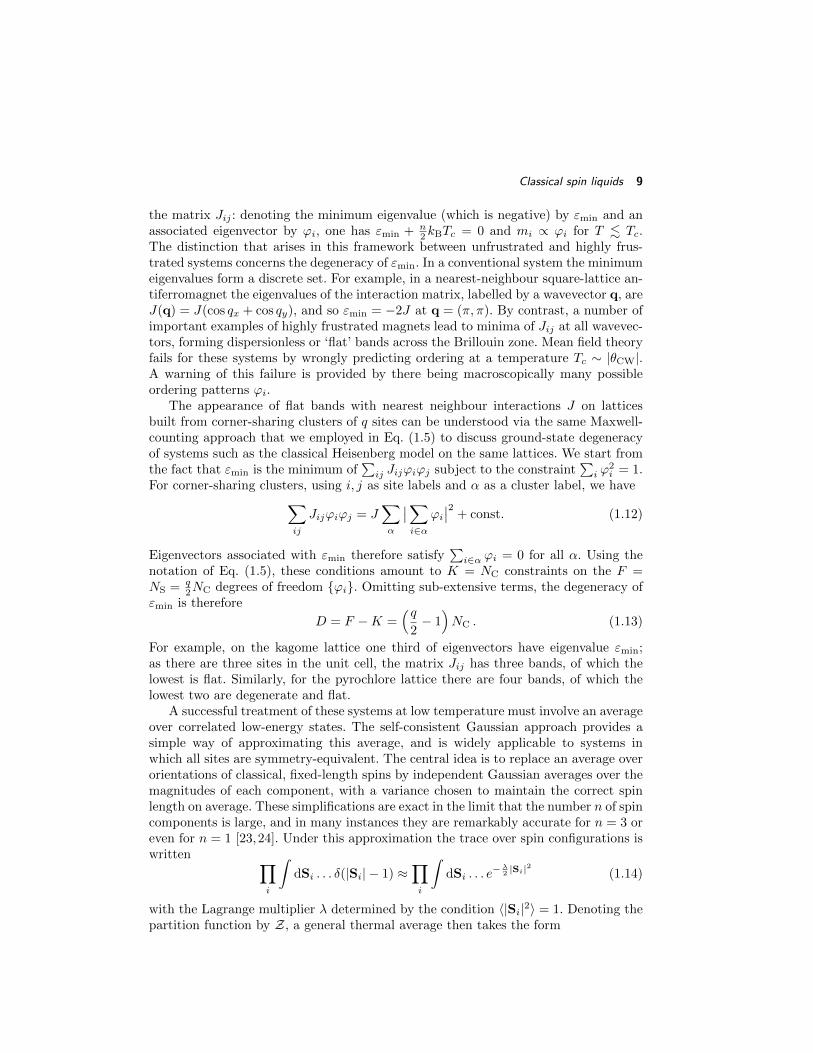
the matrix Jij : denoting the minimum eigenvalue (which is negative) by εmin and anassociated eigenvector by ϕi, one has εmin + n

2 kBTc = 0 and mi ∝ ϕi for T . Tc.The distinction that arises in this framework between unfrustrated and highly frus-trated systems concerns the degeneracy of εmin. In a conventional system the minimumeigenvalues form a discrete set. For example, in a nearest-neighbour square-lattice an-tiferromagnet the eigenvalues of the interaction matrix, labelled by a wavevector q, areJ(q) = J(cos qx + cos qy), and so εmin = −2J at q = (π, π). By contrast, a number ofimportant examples of highly frustrated magnets lead to minima of Jij at all wavevec-tors, forming dispersionless or ‘flat’ bands across the Brillouin zone. Mean field theoryfails for these systems by wrongly predicting ordering at a temperature Tc ∼ |θCW|.A warning of this failure is provided by there being macroscopically many possibleordering patterns ϕi.

The appearance of flat bands with nearest neighbour interactions J on latticesbuilt from corner-sharing clusters of q sites can be understood via the same Maxwell-counting approach that we employed in Eq. (1.5) to discuss ground-state degeneracyof systems such as the classical Heisenberg model on the same lattices. We start fromthe fact that εmin is the minimum of

∑ij Jijϕiϕj subject to the constraint

∑i ϕ

2i = 1.

For corner-sharing clusters, using i, j as site labels and α as a cluster label, we have∑ij

Jijϕiϕj = J∑α

∣∣∑i∈α

ϕi∣∣2 + const. (1.12)

Eigenvectors associated with εmin therefore satisfy∑i∈α ϕi = 0 for all α. Using the

notation of Eq. (1.5), these conditions amount to K = NC constraints on the F =NS = q

2NC degrees of freedom ϕi. Omitting sub-extensive terms, the degeneracy ofεmin is therefore

D = F −K =(q

2− 1)NC . (1.13)

For example, on the kagome lattice one third of eigenvectors have eigenvalue εmin;as there are three sites in the unit cell, the matrix Jij has three bands, of which thelowest is flat. Similarly, for the pyrochlore lattice there are four bands, of which thelowest two are degenerate and flat.

A successful treatment of these systems at low temperature must involve an averageover correlated low-energy states. The self-consistent Gaussian approach provides asimple way of approximating this average, and is widely applicable to systems inwhich all sites are symmetry-equivalent. The central idea is to replace an average overorientations of classical, fixed-length spins by independent Gaussian averages over themagnitudes of each component, with a variance chosen to maintain the correct spinlength on average. These simplifications are exact in the limit that the number n of spincomponents is large, and in many instances they are remarkably accurate for n = 3 oreven for n = 1 [23,24]. Under this approximation the trace over spin configurations iswritten ∏

i

∫dSi . . . δ(|Si| − 1) ≈

∏i

∫dSi . . . e

−λ2 |Si|2

(1.14)

with the Lagrange multiplier λ determined by the condition 〈|Si|2〉 = 1. Denoting thepartition function by Z, a general thermal average then takes the form


〈. . .〉 = Z−1

∫dSi . . . e−

12

∑ij Si(βJij+λδij)Sj . (1.15)

In particular, the spin correlator is

〈Si · Sj〉 = n[(βJ + λ)−1

]ij

(1.16)

and λ satisfies

n[(βJ + λ)−1

]ii≡ n

NSTr

1

(βJ + λ)= 1 . (1.17)

If the minimum eigenvalues of J form a flat band, then in the low-temperature limit(βJ + λ)−1 is proportional to the projector P onto this band, so that 〈Si · Sj〉 ∝ Pij .In many of the systems we are concerned with (those with a Coulomb phase: seeSec. 1.4.2), Pij falls off at large separation rij as Pij ∼ r−dij , where d is the spatialdimension.

1.2.2 The triangular lattice Ising antiferromagnet and height models

Moving beyond these simple approximations, we would like to find a description oflow-energy spin configurations that respects microscopic constraints imposed by theHamiltonian but is amenable to coarse graining. An early and illuminating exampleis provided by a mapping which we now describe, from the triangular lattice Isingantiferromagnet to a height model.

As background, we note that this Ising model (probably the first highly frustratedmagnet to be studied in detail [25]) has a macroscopically degenerate ground state,and ground-state spin correlations that are known from an exact solution to decay withdistance as r−1/2 . In ground states every elementary triangle of the lattice has twospins parallel and one antiparallel. Degeneracy arises because many such configurationsinclude some spins that are subject to zero net exchange field and can therefore bereversed at zero energy cost, as illustrated in Fig. 1.5 (left). To avoid confusion, weshould point out that the degeneracy on this lattice is specific to the Ising model, andnot a consequence of flat bands.

h−1

h+2h+1

h+1

h

h B

h=2

h=1

h=3

h=4

h=5

h=6

C

A

Fig. 1.5 Triangular lattice Ising antiferromagnet spin configurations. Left: state with a flip-

pable spin, marked with a circle. Centre: mapping from spins to heights at sites. Right:

mapping from spin orientations on the three sublattices (marked A, B and C) to triangle

heights in flat states.

Classical spin liquids 11

Spin configurations can be mapped onto a new variable, termed a height field, insuch a way that the ground-state condition in the spin model translates into a conditionthat the height field is single-valued. The mapping associates an integer height hi witheach site i [26,27]. To describe it, we introduce a direction on each bond of the latticein such a way that there is (say) anticlockwise circulation around ‘up’ triangles andclockwise circulation around ‘down’ triangles. With the height of an origin site chosenarbitrarily, the height change on traversing a bond in the positive direction is +1 ifthe bond links antiparallel (unfrustrated) spins, and −2 if it links parallel (frustrated)spins, as illustrated in Fig. 1.5 (centre). A convenient further stage is to define heightsh(r) at the centres of triangles that are averages of the three values at corners: seeFig. 1.5 (right).

h+1h

h+1h−1

h h+1

h

h−2

h−2

h−3h−1

h

h

h+1

Fig. 1.6 Triangular lattice Ising antiferromagnet spin configurations and mappings to height

field. Left: state with flippable spin generating a flat height field (with the value h at all

triangle centres). Right: spin state without flippable spins, that generates a height field with

maximum gradient (heights at triangle centres decrease by 1 on going from any triangle to

its right-hand neighbour).

As demonstrated with examples in Fig. 1.6, configurations with a flippable spinare locally flat, and those in which the gradient of the height field is maximal have noflippable spins. These facts motivate a coarse-grained theory in which h(r) is takento be a real-valued function of a continuous coordinate, with an entropic weight onconfigurations that (in the first approximation) has the form

P [h(r)] = Z−1e−H (1.18)

where

H =K

2

∫d2r|∇h(r)|2 (1.19)

and Z is the usual normalisation. The inverse mapping between spins and heights(modulo 6) is shown in Fig. 1.5 (right) for the six distinct flat states. It has thealgebraic form

S(r) ' cos(πh(r)/3 + ϕα), (1.20)

where we have omitted higher Fourier components of h(r), and the phase ϕα takes thevalues 0,±2π/3 depending on the sublattice α.


The height field h(r) has fluctuations that diverge logarithmically with separation,as we see from an explicit calculation. For a system of size L × L, define the Fouriertransform

hq =1

L

∫d2r eiq·rh(r) so that H =

K

2

∑q

q2|hq|2 .

Then, with short-distance cut-off a,

〈[h(0)− h(r)]2〉 =2

L2

∑q

(1− cosq · r)〈|hq|2〉

=1

2π2

∫d2q

1− cosq · rKq2

' 1

πKln(r/a) . (1.21)

Putting these ingredients together, we can evaluate the spin correlator using thecoarse-grained theory. For two sites on the same sublattice we obtain

〈σ(0)σ(r)〉 ∝ 〈eiπ3 [h(0)−h(r)]〉 = e−π2

18 〈[h(0)−h(r)]2〉 = (r/a)−π/18K . (1.22)

The power-law form illustrates the consequences of large but strongly correlated ground-state fluctuations, and a comparison with exact results for the Ising model fixes thevalue of the height model stiffness as K = π/9.

The leading approximation that has been made in using the height model to repre-sent the triangular lattice Ising antiferromagnet is to treat h(r) as a real, rather thaninteger-valued field. To correct this we can consider the replacement H → H + H1

with H1 = −g∫

d2r cos 2πh(r), so that values of h(r) close to integers are preferred.One finds that H1 is an irrelevant perturbation at the renormalisation group fixedpoint represented by H if K < π/2, as is the case for the height model that representsthe triangular lattice Ising antiferromagnet. Changes to the Ising model (for example,higher spin [27]) may increase K so that H1 is relevant. The height field than locks toa particular integer value, representing long-range order of the Ising spins.

Excitations out of the ground state have an attractively simple description inheight-model language. From the rules of Fig. 1.5 we see that if the three Ising spinsof an elementary triangle have the same orientation, the height field is no longer ev-erywhere single-valued: it changes by ±6 on encircling the triangle that carries theexcitation. A single spin flip can introduce such excitations into a ground-state config-uration only as vortex anti-vortex pairs vortices, since a local move leaves the distantheight field unchanged. A vortex and anti-vortex can be separated by additional spinflips without further increase in exchange energy, and constitute our first example ofa fractionalised excitation.

Vortices are dilute at low temperature, because they have an energy cost 4J . Theirpresence also changes the number of ground states available to the system, and so theyhave an entropy cost. This can be calculated within the height description. A vortex

Classical dimer models 13

at the origin leads to an average height gradient at radius r of |∇h(r)| = 6/(2πr). Ina system of linear size L this generates a contribution to H of

K

2

∫d2r |∇h(r)|2 =

9K

πln(L/a) . (1.23)

Similarly, the presence of a vortex anti-vortex pair at fixed positions with separationr has an entropy cost that depends on their separation. As a consequence, the pair issubject to an entropic attractive potential V (r) ' 9K

π ln(r/a).The entropy cost for vortices should be compared with the entropy gain 2 ln(L/a)

arising from translations: vortex anti-vortex pairs are unbound if 9K/π < 2, as is thecase here. In the setting of the Ising model, this means that the power-law correlationsof the ground state are cut off at non-zero temperature by a finite correlation length,set by the vortex separation. This correlation length is much larger than the latticespacing if T J/kB, and it diverges as T → 0.

In summary, the triangular lattice Ising antiferromagnet provides an illustrationof a system that, in its ground state, combines finite entropy with long-range corre-lations. The height model shows how these features can be captured in a long-wavelength description. The physics of the triangular lattice Ising antiferromagnet at lowtemperature, including power-law correlations and fractionalised excitations, has im-portant generalisations to other systems, including most notably spin ice. In addition,some of the main theoretical tools used in a long-wavelength description of these gen-eralised problems are extensions of the ones underlying the height model. Many ofthese ideas are exemplified in classical dimer models, which we now introduce.

1.3 Classical dimer models

Classical dimers models [28–30] offer a setting in which to discuss some general featuresof the statistical physics of systems that are both highly degenerate and stronglyconstrained. They are important in their own right and also serve as the foundationfor a treatment of quantum spin liquids using quantum dimer models.

h−1

h

h−2

h−3

Fig. 1.7 States of square lattice dimer model. Left: close-packed configuration. Centre: local

rearrangement. Right: mapping to height model.

1.3.1 Introduction

The configurations of a dimer model are close-packed coverings of a lattice, with dimersarranged on bonds in such a way that there is, in the simplest case, exactly one


dimer touching each lattice site. Examples are shown in Fig. 1.7. Entropy arises fromrearrangements of dimers. Consider, in an initial covering, a closed loop of bonds thatare alternately empty and occupied by dimers. The configuration on this loop can beflipped, exchanging empty and occupied bonds, independently of the configurationson other loops that do not intersect this one.

Close-packed dimer configurations on a planar lattice admit a height representationprovided the lattice is bipartite. Let z be the coordination number of the lattice, andintroduce the dual lattice, which has sites at the centres of the plaquettes of theoriginal lattice, and links intersecting the edges of these plaquettes. The height field isdefined at sites of the dual lattice: traversing in (say) an anti-clockwise direction theplaquettes of the dual lattice that enclose A-sublattice sites of the original lattice, wetake the height difference to be ∆h = +1 on crossing an empty bond, and ∆h = 1− zon crossing the occupied bond, as in Fig. 1.7 (right). A simple generalisation is to takedimer configurations in which exactly n dimers touch each site. Then ∆h = +n forempty bonds and n − z for occupied ones. These choices ensure that the height fieldis single-valued

There is in fact an exact correspondence between close-packed dimer configurationson the hexagonal lattice and ground states of the triangular lattice Ising antiferromag-net. To establish this, note that the hexagonal lattice has as its dual the triangularlattice. Under the correspondence, dimers on the hexagonal lattice lie across frustratedbonds of the triangular lattice, as in Fig. 1.8. In a ground state of the Ising model, theexchange interaction on exactly one edge of every elementary triangle is frustrated, andso in the corresponding dimer covering, every site of the hexagonal lattice is touchedby exactly one dimer.

Fig. 1.8 The hexagonal lattice dimer model and its correspondence with ground states of

triangular lattice Ising antiferromagnet.

1.3.2 General formulation

While the mapping from dimer coverings to a height field is particular to two-dimensional,bipartite lattices, it can be reformulated in language that generalises directly to higherdimensions [31]. To do so, we first make use of the bipartite nature of the lattice todefine an orientation convention on nearest neighbour bonds, taking the direction tobe from (say) the A-sublattice to the B-sublattice. We then define for each dimer con-figuration a flux in this direction on each link, which (for a lattice with coordinationnumber z) is 1− z on links occupied by a dimer, and +1 on unoccupied links.


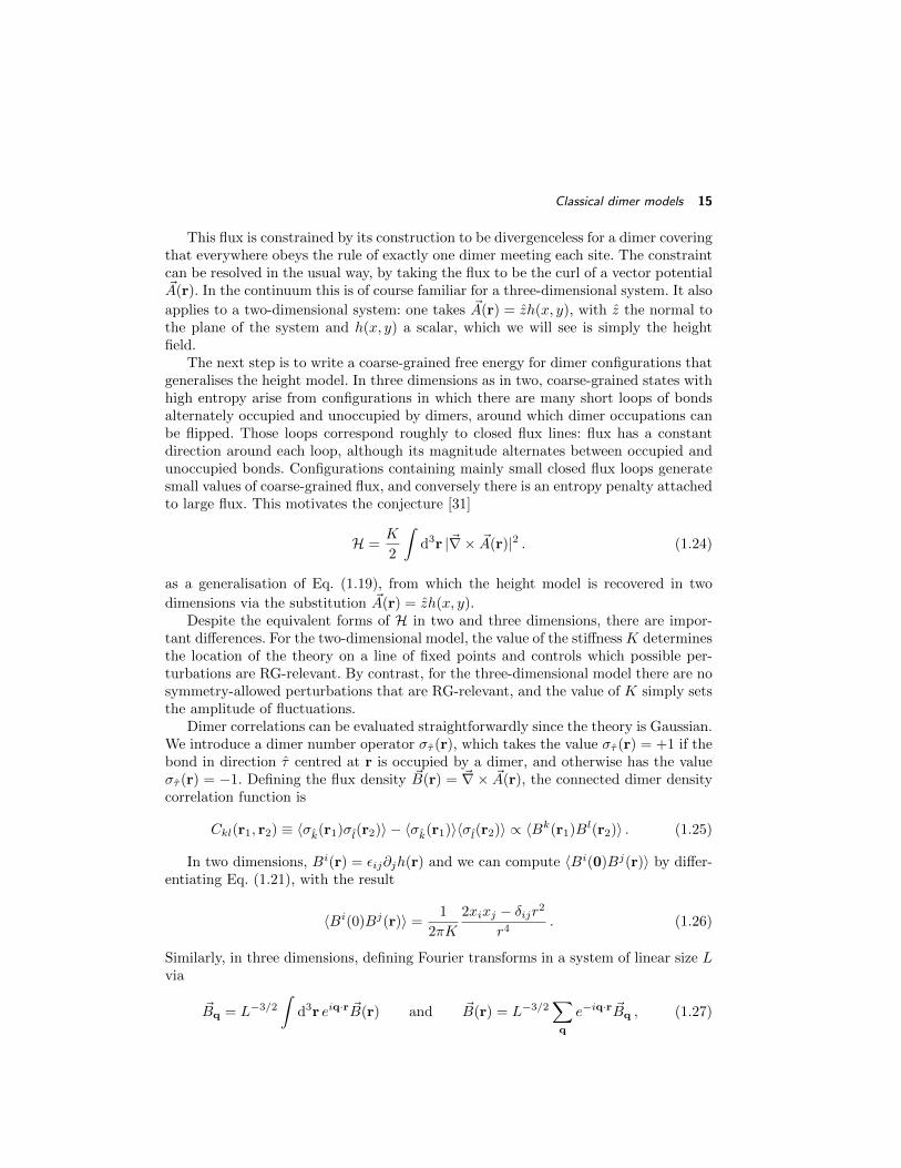
This flux is constrained by its construction to be divergenceless for a dimer coveringthat everywhere obeys the rule of exactly one dimer meeting each site. The constraintcan be resolved in the usual way, by taking the flux to be the curl of a vector potential~A(r). In the continuum this is of course familiar for a three-dimensional system. It also

applies to a two-dimensional system: one takes ~A(r) = zh(x, y), with z the normal tothe plane of the system and h(x, y) a scalar, which we will see is simply the heightfield.

The next step is to write a coarse-grained free energy for dimer configurations thatgeneralises the height model. In three dimensions as in two, coarse-grained states withhigh entropy arise from configurations in which there are many short loops of bondsalternately occupied and unoccupied by dimers, around which dimer occupations canbe flipped. Those loops correspond roughly to closed flux lines: flux has a constantdirection around each loop, although its magnitude alternates between occupied andunoccupied bonds. Configurations containing mainly small closed flux loops generatesmall values of coarse-grained flux, and conversely there is an entropy penalty attachedto large flux. This motivates the conjecture [31]

H =K

2

∫d3r |~∇× ~A(r)|2 . (1.24)

as a generalisation of Eq. (1.19), from which the height model is recovered in two

dimensions via the substitution ~A(r) = zh(x, y).Despite the equivalent forms of H in two and three dimensions, there are impor-

tant differences. For the two-dimensional model, the value of the stiffness K determinesthe location of the theory on a line of fixed points and controls which possible per-turbations are RG-relevant. By contrast, for the three-dimensional model there are nosymmetry-allowed perturbations that are RG-relevant, and the value of K simply setsthe amplitude of fluctuations.

Dimer correlations can be evaluated straightforwardly since the theory is Gaussian.We introduce a dimer number operator στ (r), which takes the value στ (r) = +1 if thebond in direction τ centred at r is occupied by a dimer, and otherwise has the valueστ (r) = −1. Defining the flux density ~B(r) = ~∇× ~A(r), the connected dimer densitycorrelation function is

Ckl(r1, r2) ≡ 〈σk(r1)σl(r2)〉 − 〈σk(r1)〉〈σl(r2)〉 ∝ 〈Bk(r1)Bl(r2)〉 . (1.25)

In two dimensions, Bi(r) = εij∂jh(r) and we can compute 〈Bi(0)Bj(r)〉 by differ-entiating Eq. (1.21), with the result

〈Bi(0)Bj(r)〉 =1

2πK

2xixj − δijr2

r4. (1.26)

Similarly, in three dimensions, defining Fourier transforms in a system of linear size Lvia

~Bq = L−3/2

∫d3r eiq·r ~B(r) and ~B(r) = L−3/2

∑q

e−iq·r ~Bq , (1.27)


one finds

〈BiqBjk〉 =

1

K

(δij −

qiqjq2

)δq,−k (1.28)

and hence [31]

〈Bi(0)Bj(r)〉 =1

4πK

3rirj − δijr2

r5. (1.29)

We see that, while dimer coverings of bipartite lattices described by this coarse-grained theory are disordered, with finite entropy density and no local symmetrybreaking, the constraints of close packing and hard-core exclusion lead to power-lawcorrelations with a characteristic form. States with these correlations are known asCoulomb phases [36].

1.3.3 Flux sectors, U(1) and Z2 theories

It is an important feature of of dimer models on bipartite lattices that the configurationspace divides into sectors which are not connected by any local dimer rearrangements.For a system with periodic boundary conditions, these sectors are distinguished bythe values of total flux encircling the system in each direction. Dimer rearrangementsaround short loops leave these global fluxes unchanged, and the order characterisedby the fluxes is referred to as topological.

This definition of global flux is illustrated in Fig. 1.9. Let N↑ be the number ofdimers that cross the line A-B on upward-directed links, and let N↓ be the number ondownward-directed links. (In d dimensions, this line is replaced by a (d−1)-dimensionalhypersurface.) Then the net flux across the line (or hypersurface) is Φ = (1− z)(N↑−N↓), where the coordination number is z = 4 for the square lattice. The value of Φis unchanged by flipping dimers on contractable loops (ones that do not wrap aroundthe system), as shown in Fig. 1.9 (ii) and (iii). Moreover, although microscopic valuesof the flux Φ are discrete, this restriction is unimportant after coarse-graining: fora three-dimensional system in the continuum limit we can view ~A(r) as the vector

potential for a continuous-valued flux density ~B(r) = ~∇ × ~A(r). Then Eq. (1.24) issimply the action for a U(1) gauge theory.

A B

(i) (ii) (iii)

Fig. 1.9 Flux sectors in a bipartite lattice dimer model. (i) Orientation convention on edges

of the lattice. (ii) A dimer flip on the marked loop changes both N↑ and N↓ by 1. (iii) A

dimer flip on a different marked loop changes local contributions to N↑ by ±1 but leaves its

net value unaltered.

Dimer models can equally be defined on lattices that are not bipartite, but the long-distance physics in these cases is very different. For these systems it is not possible to


define a local divergenceless flux, and sectors of configuration space are labelled by Z2

rather than U(1) quantum numbers. For a d-dimensional system there are d of thesequantum numbers, giving the parity of the number N of dimers intersecting a setof (d − 1)-dimensional hypersurfaces. A change in the dimer configuration producedby flipping dimers on a contractable loop leaves these parities unchanged. To seethis, note that the loop intersects the surface an even number of times, and considerthe contribution to overall parity from two successive interactions. If the length of theloop between the crossings is even, then both intersections make the same contribution(both 0 or both 1) to N , and the combined contribution modulo 2 is unchanged whendimers on the loop are flipped; alternatively, if the length between crossings is odd,the two interactions make opposite contributions (one 0 and the other 1) to N , andtheir individual contributions swap when dimers are flipped.

It is known from exact solutions for two-dimensional lattices using Pfaffians [33],and from Monte Carlo simulations in three dimensions [31], that dimer-dimer correla-tions generically decay exponentially with separation for close-packed dimer coveringsof non-bipartite lattices.

1.3.4 Excitations

Vortices in the height representation can arise from defects of more than one typein the dimer covering. One of these is obvious from the mapping between triangularlattice spin configurations and hexagonal lattice dimer configurations: a triangle inwhich three spins have the same orientation maps to a site of the hexagonal lattice atwhich three dimers meet. This excitation acts as a source or sink of the flux we haveintroduced, depending on which sublattice the site belongs to.

Fig. 1.10 Monomers in the hexagonal lattice dimer model. Left: dimer replaced with two

monomers. Right: separation of the monomers by dimer flips.

An alternative type of height vortex, which is of interest for the dimer model, isone in which a dimer is removed, or equivalently, replaced by two monomers, as inFig. 1.10. The two monomers can be separated by subsequent dimer moves, one alwaysremaining on the A-sublattice and the other on the B-sublattice. The two monomersare represented by a vortex anti-vortex pair in the height model. From the argumentsleading to Eq. (1.23), we see that such a pair will be subject to an attractive entropicpotential that increases logarithmically with separation.

This entropic potential is a natural consequence of the fact that a monomer acts asa source for flux ~B(r) if it is on one sublattice, and as a sink if it is on the other sublat-tice, and the logarithmic dependence on distance is characteristic of the Coulomb in-


teraction in two dimensions. Similarly, the entropic potential V (r) in three dimensionsbetween a pair of monomers on opposite sublattices at separation r can be evaluatedstraightforwardly within the continuum description of Eq. (1.24). The presence of the

excitations results in an additional contribution to ~B(r). Let ~Bsource be the field con-

figuration that minimises H in the presence of the pair, and write ~B(r) = ~Bsource +δ ~B.

Since H is quadratic in ~B(r), integration over fluctuations δ ~B yields a weight that isunaffected by the presence or separation of the pair. We can therefore determine V (r)

simply from ~Bsource, and by the usual arguments of electrostatics we find

V (r) = − K

4πr. (1.30)

Since the entropic cost of separating the pair to infinity is bounded, monomer excita-tions in a Coulomb phase in three dimensions are deconfined.

In a dimer model that has long-range order, monomers are subject to a potentialthat grows much more rapidly with separation. For example, in two dimensions thecoarse-grained height field steps between different pinned values along a line joiningthe vortex anti-vortex pair. This generates an interaction that is linear in separation,and the same result holds in three dimensions.

On non-bipartite lattices in both two and three dimensions the entropic interactionpotential between a pair of monomers approaches a finite limiting value exponentiallyfast with increasing separation, provided the dimer coverings are disordered. The de-confinement of monomers is an important property distinguishing Z2 from U(1) phasesin two dimensions.

It is characteristic of topologically ordered systems that transitions between groundstates of a system on a torus can be engineered by a sequence of steps, consisting ofthe generation of a pair of excitations, followed by transport of one excitation aroundthe torus, and ending with recombination. For a dimer model the first of these steps isthe replacement of a dimer by a pair of monomers. The flux quantum number for thedimer covering is changed if one of these monomers is transported around the torusby flipping dimers, until the two monomers are again adjacent and can be replacedwith a dimer.

1.4 Spin ice

The spin-ice materials Ho2Ti2O7 and Dy2Ti2O7 provide fascinating realisations of theIsing antiferromagnet on the pyrochlore lattice, in which both the nearest-neighbourand the long-range dipolar contributions to spin interactions make very distinctivecontributions to the physical behaviour [34]. In this section we give an overview of theresulting physics, making use of some of the general ideas developed in our discussionof Coulomb phases.

1.4.1 Materials

Isolated Ho3+ and Dy3+ ions have high angular momentum (J = 8 and J = 15/2respectively) and large magnetic moments (10µB in both cases). In spin-ice materialsthe effect of the electrostatic environment of the rare earth ions is to split the 2J + 1

Spin ice 19

degenerate states of the free ions into crystal field levels. Approximating the crystalfield Hamiltonian by −D(Jz)

2, one has for positive D a ground state doublet MJ =±J . Since excited crystal field levels are several hundred kelvin higher in energy andthe scale for interactions between spins is only a few kelvin, the moments can berepresented by Ising pseudospins Si. The easy axis at given a site is the local 〈111〉direction joining the centres of the two tetrahedra that share it, and so momentsare directed either into or out of tetrahedra, as shown in Fig. 1.11. The centres oftetrahedra of the pyrochlore lattice lie on a diamond lattice, which is bipartite. Wetake the convention that Si = +1 represents a spin directed out of a tetrahedron onthe A-sublattice.

Fig. 1.11 Magnetic moments at sites of a pyrochlore lattice, orientated along local 〈111〉 axes

in a ‘two-in two-out’ state. In later figures, for ease of drawing, we represent the tetrahedron

in the flattened way shown on the right.

Strikingly, frustration arises from the combination of this local easy-axis anisotropywith ferromagnetic nearest-neighbour coupling (θCW ' +1.9K and +0.5K for the Hoand Dy compounds, respectively), and energy is minimised for the two-in two-outstates of the type illustrated in Fig. 1.11 [35]. The term spin ice is chosen becausethese spin arrangements mimic the proton positions in water-ice. As the values ofθCW are relatively small and the magnetic moments are large, long-range dipolarinteractions are important in addition to the nearest neighbour coupling; we discusstheir consequences in Sec. 1.4.3, but first examine the physics of the nearest-neighbourmodel.

1.4.2 Coulomb phase correlations

We would like to develop a description of ground states of the nearest-neighbour modelfor spin ice that is analogous to the height representation for the triangular lattice Isingantiferromagnet, and amenable to coarse-graining. The approach [24,36] parallels theone introduced for three-dimensional dimer models in Sec. 1.3

In order to describe in a general way the ideas that are involved, it is useful tointroduce some terminology. For a given system of corner-sharing frustrated clusters,we will be concerned with two types of lattice. One is simply the magnetic lattice onwhich the moments reside, also known as the medial lattice, and we denote this by L.The other is the cluster (or simplex) lattice, also known as the pre-medial or parentlattice, which we denote by B. The sites of L lie at the midpoints of the links of B,


and in the notation of graph theory, L is the line graph associated with the graph B.For spin ice, L is the pyrochlore lattice and B is the diamond lattice. Alternatively, ifwe take L to be the kagome lattice, then B is the hexagonal lattice.

A key requirement in the following is that B should be a bipartite lattice. We canthen orient the links of B, say from sites of sublattice A to sites of sublattice B. Letei be the unit vector in this direction on link i, and note that i also labels a site of L.

The central idea is to introduce a vector field ~B, defined on the links of B, that isa representation of a configuration of Ising spins Si on L, and given by the relation

~Bi = Siei . (1.31)

The field ~B is a useful construction because the ground-state condition for spin ice –that two spins are directed into each tetrahedron, and two are directed out – translatesinto the condition that ~B has zero lattice divergence at each node of B. The field ~B istherefore an emergent gauge field.

Fig. 1.12 Ground-state configurations on the two-dimensional pyrochlore lattice. Left: a

state containing short flippable loops of spins. Centre: the state obtained from this by flipping

four spins on the marked loop. Right: a state with no flippable spins and maximal flux ~B.

The next step is to conjecture a probability distribution for a coarse-grained versionof ~B. Some ground states contain short loops of flippable spins: closed loops on the Blattice, around which all spins are directed in the same sense. Further ground stateswith a similar coarse-grained ~B are obtained by reversing all the spins on one of theseloops, and so entropy favours states with a high density of short loops, as illustratedin Fig. 1.12 using a two-dimensional version of the pyrochlore lattice. These consider-ations suggest that states in which ~B is large have lower entropy. This motivates forthe probability distribution the form

P [ ~B(r)] = Z−1e−H (1.32)

with

H =K

2

∫d3r| ~B(r)|2 , (1.33)

where ~B(r) is a continuum field, subject to the ground-state constraint ~∇ · ~B = 0,just as in our earlier discussion of Coulomb phases in dimer models. Indeed, spin iceground states can be represented directly by dimer coverings on the diamond latticewith two dimers touching every site, simply by using dimers on B to represent spins

Spin ice 21

Si = +1 on L. Ground state spin correlations in spin ice therefore have the dipolarform given in Eq. (1.29).

(a)

0 0

r

r

(b)

Fig. 1.13 Illustration of the origin of dipolar correlations in spin ice. Spins at 0 and r are

correlated if a flux line of the emergent field ~B(r) passes through both sites. The orientations

of the flux line at the two sites depends on the direction of their spatial separation, so that

for (a) 〈S0Sr〉 > 0 and for (b) 〈S0Sr〉 < 0.

The angular dependence of this correlator means that a pair of well-separated spinson sites of the same sublattice of L (and hence with the same orientation for e at bothsites) are positively correlated if their separation vector r is in the direction of e,but most likely to be anti-aligned if r is perpendicular to e. Such behaviour can beunderstood by considering the geometry of flux lines of the emergent gauge field ~B(r).A spin configuration in which σ0 = +1 is one with a flux line passing through the originin the direction e, and this flux line must close on itself since the field is divergenceless.The spin σr is correlated with σ0 only in those configurations in which the same fluxline passes through r, and the most likely orientation of this flux line at r depends onthe relative directions of r and e, as shown in Fig. 1.13. The reciprocal space signature,Eq. (1.28), of these correlations consists of so-called pinch-point structures, sharp butwithout divergences, observed in elastic neutron diffraction [9].

It is interesting to connect the results obtained from a continuum treatment of theemergent gauge field to those arising from the self-consistent Gaussian approximationof Section 1.2.1. Adopting the sublattice labels and axis orientations shown in Fig. 1.14,the net Ising moment M and flux components Bx, By and Bz arising from a spinconfiguration S1, S2, S3 and S4 on the four sublattices are [37]

MBxByBz

=1

2

1 1 1 11 1 −1 −11 −1 1 −11 −1 −1 1

·S1

S2

S3

S4

. (1.34)

The statistical weight of fluctuations is determined within the self-consistent Gaussianapproximation by their energy and by a Lagrange multiplier λ. From Eq. 1.1, theenergy per unit cell of a configuration is J

2M2. Moreover, the net Ising moment M is

simply the lattice version of ~∇· ~B. In continuum notation, Eq. 1.15 therefore amountsto a Boltzmann factor e−H with

H =

∫d3r

λ

2| ~B(r)|2 +

βJ

2M2

. (1.35)


In this way we see that λ sets the value of the stiffness K for fluctuations of ~B(r). We

also recover the condition ~∇ · ~B(r) = 0 in the low-temperature limit βJ →∞.

x

yz

1

2

3

4

Fig. 1.14 Choice of axes and sublattice labels for the pyrochlore lattice.

1.4.3 Monopoles

Some beautiful physics becomes apparent when we examine configurations of spin icethat do not obey the two-in two-out rule for ground states of the model with nearestneighbour interactions [38]. Consider the configuration obtained from a ground state byreversing a single spin. As illustrated in Fig. 1.15, two separate elementary excitationsare obtained from it through further spin reversals. Because, like vortex excitationsin the triangular lattice Ising antiferromagnet, these elementary excitations are notproduced singly by local spin flips, they are said to be fractionalised. Moreover, sinceone member of the pair is a source for the emergent gauge flux, and the other a sink,they form a monopole anti-monopole pair.

−

+

−

+ +

−

Fig. 1.15 Generation of a monopole anti-monopole pair from ground state of two-dimen-

sional spin ice, and their separation, by successive spin flips.

The energy of a monopole anti-monopole pair arising from exchange interactionsis independent of their separation in a nearest neighbour model. There is, however,an entropic interaction between the pair, since the number of ground states availableto the background spins depends on the separation r of the excitations. The entropicpotential V (r), as for monomers in the Coulomb phase of a three-dimensional dimermodel on a bipartite lattice, is given by Eq. (1.30). Likewise, since the entropic costof separating the pair to infinity is bounded, monopole excitations are deconfined.

Spin ice 23

1.4.4 Dipolar interactions

Our treatment of spin ice to this point has omitted the long-range part of dipolarinteractions. Clearly, its inclusion will lift the high degeneracy of ground states of thenearest neighbour model, and one might expect that it would simply set an unwelcomelimit on the physics we have discussed so far. Rather than being just a bug, however,dipolar interactions turn out to add a spectacular feature to spin-ice physics [38].

A very convenient framework for thinking about dipolar effects is provided by anapproximation known as the dumbbell model. Here, in the first instance, magneticdipoles µ of atomic size are replaced by ‘dumbbells’ of positive and negative magneticcharge Q/2 at a separation a equal to the distance between the centres of adjacenttetrahedra of the lattice. Setting the dipole moment of the dumbbell equal to themicroscopic moment, the leading contribution to long-range interactions is capturedexactly. The power of this description stems from the fact that, for all ground states ofthe nearest-neighbour model, the positive and negative magnetic charges at the centreof each tetrahedron cancel. In turn, this fact is a demonstration that the leadingcontribution to the energy from dipolar interactions is the same for all these states.Subleading terms follow from the multipole expansion and fall off with distance asr−5. The estimated ordering temperature of spin-ice materials, Tc . 0.2 θCW, is ratherlow for that reason [39]. Such ordering is not observed under ordinary experimentalconditions because spin dynamics is very slow at low temperature.

Turning to monopole excitations, the dumbbell model serves to expose a strikingconsequence of dipolar couplings, since dumbbell charges fail to cancel in tetrahedrathat contain these quasiparticles. As a result, a well-separated monopole anti-monopolepair is subject to a Coulomb interaction

U(r) = −µ0Q2

4πr(1.36)

of magnetic origin. The charge Q is related to the atomic dipole moment and the

+

−

−+

+

0

− −

+

+

+

2

Fig. 1.16 The dumbbell approximation. Dipoles are replaced with a dumbbell of opposite

charges at finite separation, as shown at the top. If this separation is chosen to be the distance

between tetrahedron centres, then two-in two-out tetrahedra are charge neutral (bottom left)

but one-in three-out tetrahedra have net charge (bottom right).

lattice spacing by Q = 2µ/a, and the monopole chemical potential is fixed by the


nearest-neighbour contributions to spin interactions. Note that while the entropic anddipolar contributions to monopole interactions (Eqns. 1.30 and 1.36) have the samedependence of separation, the entropic one makes a temperature-independent contri-bution to Boltzmann weights and so the dipolar one is dominant at low temperature.The magnetic Coulomb interaction between monopoles is a remarkable example of anemergent longer-range interaction (1/r) arising from shorter-range (1/r3) microscopicinteractions. It appears because of the interplay between these microscopic interactionsand the correlations of the Coulomb phase, and it stands in contrast to the familiarsituation (for example, in a plasma) in which correlations serve to screen long-rangemicroscopic interactions, leaving only a short-range effective potential.

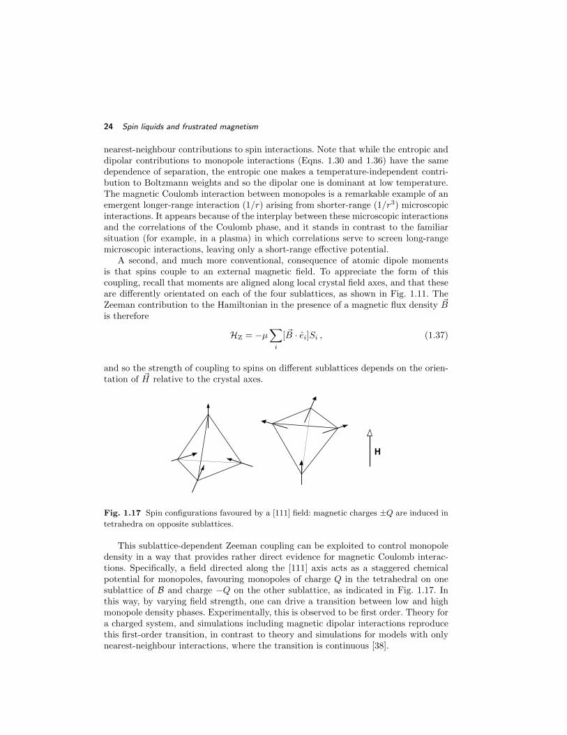
A second, and much more conventional, consequence of atomic dipole momentsis that spins couple to an external magnetic field. To appreciate the form of thiscoupling, recall that moments are aligned along local crystal field axes, and that theseare differently orientated on each of the four sublattices, as shown in Fig. 1.11. TheZeeman contribution to the Hamiltonian in the presence of a magnetic flux density ~Bis therefore

HZ = −µ∑i

[ ~B · ei]Si , (1.37)

and so the strength of coupling to spins on different sublattices depends on the orien-tation of ~H relative to the crystal axes.

H

Fig. 1.17 Spin configurations favoured by a [111] field: magnetic charges ±Q are induced in

tetrahedra on opposite sublattices.

This sublattice-dependent Zeeman coupling can be exploited to control monopoledensity in a way that provides rather direct evidence for magnetic Coulomb interac-tions. Specifically, a field directed along the [111] axis acts as a staggered chemicalpotential for monopoles, favouring monopoles of charge Q in the tetrahedral on onesublattice of B and charge −Q on the other sublattice, as indicated in Fig. 1.17. Inthis way, by varying field strength, one can drive a transition between low and highmonopole density phases. Experimentally, this is observed to be first order. Theory fora charged system, and simulations including magnetic dipolar interactions reproducethis first-order transition, in contrast to theory and simulations for models with onlynearest-neighbour interactions, where the transition is continuous [38].

Quantum spin liquids 25

1.5 Quantum spin liquids

We now turn to the quantum physics of frustrated magnets, where frustration is in-teresting particularly because it provides a mechanism that suppresses Neel order andpromotes alternative, quantum-disordered phases.

1.5.1 Introduction

To understand that destruction of conventional order is likely in frustrated magnets,we can examine the reduction of ordered moments in the Neel state by zero-point fluc-tuations. Within the framework of harmonic spinwave theory, we start from a classicalground state for a spin model and choose axes at each site that have z oriented along thelocal ground-state spin direction. Using the Holstein-Primakoff transformation, spinoperators are expressed in terms of bosonic ones via the relation Szr = S− a†rar. Fluc-tuations lower the ground-state moment 〈Szr 〉 = S −∆S by an amount ∆S ≡ 〈a†rar〉that can be expressed as an average over contributions from each mode. The schematicform (details depend on the system) in terms of spinwave frequencies ωk and exchangeinteraction J is [40]

∆S ∼ J

Ω

∫BZ

ddk

~ωk, (1.38)

where Ω is the Brillouin zone (BZ) volume. As we have seen in Sec. 1.1.2, frustrationpromotes macroscopic classical ground-state degeneracy and branches of soft modes.Here we find that these modes make divergent contributions to ∆S, destabilising longrange order.

Is the resulting state a quantum spin liquid? A necessary requirement is that (i) theground state leaves all symmetries of the Hamiltonian unbroken, and the absence ofNeel order is one aspect of this. To appreciate that we should demand more, consideras an example a bi-layer, square-lattice spin-half Heisenberg antiferromagnet, havingnearest neighbour exchange J within layers and J ′ between layers. This model has twophases: the ground state is Neel ordered for J ′ J , but consists of interlayer singletsfor J ′ J . Although the large J ′/J state breaks no symmetries, it is ‘ordinary’rather than ‘exotic’, in the sense that it is continuously connected to a band insulator.That is to say, there is a path in the space of Hamiltonians that connects this phaseof the spin model to a tight-binding model without interactions, that has one filledband (symmetric under layer interchange) and one empty band (antisymmetric underinterchange).

To exclude such ordinary possibilities, we make require in addition that a quantumspin liquid (ii) has half odd-integer spin per unit cell. The combination of (i) and (ii)together imply for a large class of models that a system with a gapped ground statehas topological order, as we now discuss.

1.5.2 Lieb-Schultz-Mattis theorem

Some strong constraints on the nature of ground states and excitations in spin modelsthat have half odd-integer spin per site and (at least) U(1) symmetry are revealedby the Lieb-Schultz-Mattis theorem [41]. It was originally proved for one-dimensional


models, but has subsequently been applied to quasi-one dimensional and higher di-mensional systems [42,43]. The theorem shows for a chain of length L that the energygap between the ground and first excited states vanishes as L → ∞. We know ofthree distinct ways in which this can happen. Two of them are conventional. First, ifthe model spontaneously breaks a symmetry, the ground state belongs to a low-lyingmultiplet, and splittings within the multiplet vanish as L diverges. An example is astate in which the size of the unit cell is doubled spontaneously by spin dimerisa-tion. Second, if the model has a branch of gapless excitations, the lowest excitationenergy decreases as a power of system size. This is the case for spinon excitations inthe spin-half Heisenberg chain. The third, unconventional possibility concerns systemsthat do not show symmetry breaking, and in which excitations that can be createdby local operators are gapped. For these, the implication of the theorem is that theground state belongs to a low-lying multiplet that does not originate from symmetrybreaking. Instead, it has its origin in topological order.

We will sketch the proof as it applies to the spin-half XXZ chain, and then discussmore general implications. Consider the Hamiltonian

H = J∑n

1

2[S+n S−n+1 + S−n S

+n+1] + ∆SznS

zn+1

(1.39)

for a chain of L sites with periodic boundary conditions and L even. Suppose theground state |0〉 is unique (if it is degenerate, there is nothing to prove, since the gapis zero) and denote its energy by E0. We construct a second state |ψ〉 = U |0〉 from itby acting with an operator

U = exp

(2πi

L∑n=1

n

LSzn

)(1.40)

that generates a long-wavelength twist of spin configurations about the z-axis. We willshow that 〈ψ|0〉 = 0, and will use 〈ψ|(H−E0)|ψ〉 to obtain a variational bound on theseparation in energy between the ground and first excited states of H.

To show orthogonality of |0〉 and |ψ〉, consider the effect of translations on |0〉 andon |ψ〉. Let the operator T effect translation by one lattice spacing. We have T |0〉 = |0〉since the ground state is unique. On the other hand

TU T−1 = U e−2πiL

∑n S

zn e2πiSz1 . (1.41)

The factor e−2πiL

∑n S

zn = +1 if

∑n S

zn = 0 (and there is ground-state degeneracy if∑

n Szn 6= 0), but for half-odd-integer spins the factor e2πiSz1 = −1. Hence T|ψ〉 = −|ψ〉,

and therefore 〈ψ|0〉 = 0.In order to evaluate 〈ψ|(H − E0)|ψ〉, we first examine how U transforms a single

spin operator. We have

e−iθSz

S+eiθSz

= e−iθS+ and so U†S+n S−n+1U = e2πi/LS+

n S−n+1 . (1.42)

From this we find


〈ψ|(H− E0)|ψ〉 = −J2

[1− cos(2π/L)]∑n

〈S+n S−n+1 + S−n S

+n+1〉 . (1.43)

Since the factor [1−cos(2π/L)] decreases as 1/L2 while∑n |〈S+

n S−n+1+S−n S

+n+1〉| ≤ 2L,

the energy gap separating E0 from the next eigenstate vanishes at least as fast as 1/L,which is the result we seek.

These ideas can most simply be extended to higher dimensions by considering asystem on a strip, with the width M chosen to be an odd integer so that the spinper unit cell of the strip remains half odd-integer [42]. The bound on the energy gapimplied by Eq. (1.43) is then O(M/L), which again vanishes provided we take thethermodynamic limit in an anisotropic fashion, a restriction not required in a moresophisticated approach [43].

The possibility of asymptotic degeneracy without symmetry breaking or gaplessexcitations is very striking. One route to understanding how it can arise is providedby quantum dimer models.

1.5.3 Quantum dimer models

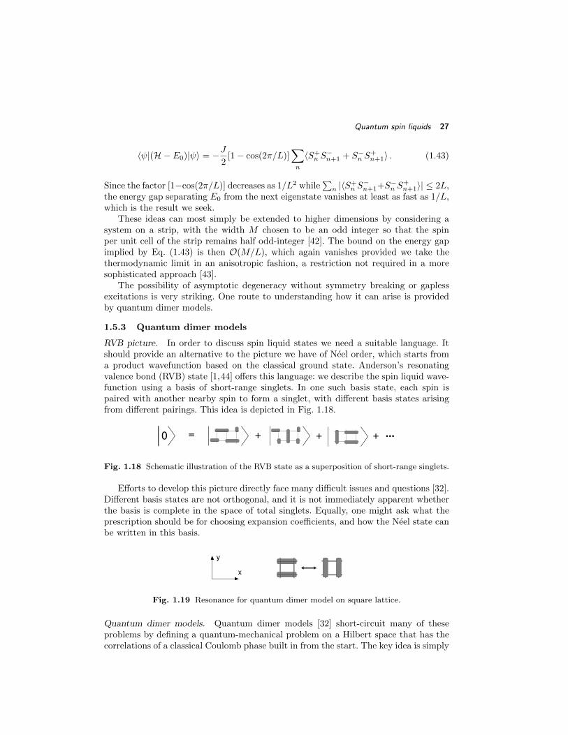
RVB picture. In order to discuss spin liquid states we need a suitable language. Itshould provide an alternative to the picture we have of Neel order, which starts froma product wavefunction based on the classical ground state. Anderson’s resonatingvalence bond (RVB) state [1,44] offers this language: we describe the spin liquid wave-function using a basis of short-range singlets. In one such basis state, each spin ispaired with another nearby spin to form a singlet, with different basis states arisingfrom different pairings. This idea is depicted in Fig. 1.18.

...+ +=0 +

Fig. 1.18 Schematic illustration of the RVB state as a superposition of short-range singlets.

Efforts to develop this picture directly face many difficult issues and questions [32].Different basis states are not orthogonal, and it is not immediately apparent whetherthe basis is complete in the space of total singlets. Equally, one might ask what theprescription should be for choosing expansion coefficients, and how the Neel state canbe written in this basis.

x

y

Fig. 1.19 Resonance for quantum dimer model on square lattice.

Quantum dimer models. Quantum dimer models [32] short-circuit many of theseproblems by defining a quantum-mechanical problem on a Hilbert space that has thecorrelations of a classical Coulomb phase built in from the start. The key idea is simply


to define an orthonormal basis |C〉 set to be the close-packed dimer coverings C ofa given lattice, so that an arbitrary state in this space has the form |ψ〉 =

∑C AC |C〉.

The other ingredient is a choice of Hamiltonian. In general it will have ‘potential’terms, which are diagonal in the dimer covering basis, and ‘kinetic’ terms, which areoff-diagonal. The form proposed for the square lattice by Rokhsar and Kivelson [32] is

H =∑−t[ |=〉〈‖|+ |‖〉〈=| ] + v[ |‖〉〈‖|+ |=〉〈=| ] . (1.44)

The notation used is intuitive although compact. Unpacking it: the sum runs overall elementary plaquettes of the lattice and the symbol |=〉〈=| denotes a projectionoperator onto states that have a horizontal pair of dimers in this plaquette. Similarly,the symbol |=〉〈‖| represents an operator that converts a horizontal pair of dimers inthis plaquette to a vertical pair, and yields zero otherwise. It therefore produces thedimer resonances shown in Fig. 1.19.

Extensions to different lattices are straightforward. For example, on the triangularlattice one allows resonances of pairs of dimers on four-site plaquettes of three types,as shown in Fig. 1.20(a), while on the honeycomb lattice three-dimer resonances arerequired [Fig. 1.20(b)]. In general, one wants to include in the kinetic energy a set ofresonances that is sufficient to connect all dimer configurations within a given U(1) orZ2 sector, but otherwise as local as possible.

(b)(a)

Fig. 1.20 Resonances for quantum dimer models on (a) triangular and (b) honeycomb lat-

tices.

The nature of the ground state of the quantum dimer model Hamiltonian (1.44)depends on the values of the parameters v and t. We will discuss only t > 0, so thatthe kinetic energy favours a nodeless wavefunction. A special role is played by theRokhsar-Kivelson (RK) point in parameter space, v = t, because here the groundstate wavefunction is given exactly by an equal-amplitude superposition |G〉 of alldimer coverings within a given sector. To see this, note that the Hamiltonian at theRK point has a form

HRK = t∑(

|‖〉 − |=〉)(〈‖| − 〈=|

)(1.45)

which is a sum of projectors with a positive coefficient. Its eigenvalues are thereforenon-negative. Moreover |G〉 is annihilated by the projection operators, and so is aneigenstate with energy zero. It is unique by the Perron-Frobenius theorem, providedthe kinetic term is ergodic within the sector.

Correlations. Knowledge of the ground state wavefunction enables us to evaluateequal-time correlation functions. In particular, the ground state expectation value ofan observable that is diagonal in the dimer basis is given by an average over dimercoverings. From this we can deduce at once that dimer correlations at the RK pointof a quantum dimer model take the power-law form characteristic of a Coulomb phase


[see Eqns. (1.26) and (1.29) for two and three dimensions, respectively] on bipartitelattices, and are exponentially decaying on non-bipartite lattices.

We can also consider the quantum dimer model in the presence of a pair of staticmonomers. At the RK point, equal amplitude superpositions of dimer coverings con-tinue to define zero energy eigenfunctions, and so the ground state energy is indepen-dent of the separation between monomers. From this one concludes that monomersare deconfined in the ground state. Consider for comparison the behaviour at infinitetemperature. In this limit (as discussed in Sec. 1.3) there is an entropic contributionto the monomer-monomer potential. It is weakly (logarithmically) divergent at largeseparations in two dimensions on bipartite lattices, giving confinement in this case. Inother cases monomers are deconfined: the potential has the Coulomb form on three-dimensional bipartite lattices, and approaches its limiting value exponentially fast withseparation on non-bipartite lattices in both two and three dimensions.

Phase diagram. Moving away from the solvable RK point, we would like to under-stand the ground-state phase diagrams of quantum dimer models on various latticesas a function of the dimensionless coupling v/t [32, 45, 46]. The behaviour in someregimes and limits is clear from simple arguments.

First, for v > t we can write H in terms of the Hamiltonian HRK at the RK pointand a non-negative remainder, as

H = HRK + (v − t)∑

|‖〉〈‖|+ |=〉〈=|. (1.46)

The so-called staggered state shown in Fig. 1.21(a) is annihilated by both terms in thisHamiltonian, and is hence the ground state for all v > t. In terms of the description ofCoulomb phases on bipartite lattices, this is the state with maximal flux. It also hasanalogues on non-bipartite lattices: see Fig. 1.21(d).

(d)(c)(b)(a)

Fig. 1.21 Some possible ordered phases for quantum dimer models: (a) staggered, (b) colum-

nar and (c) plaquette states on the square lattice; (d) staggered state on the triangular lattice.

In the opposite limit, v → −∞, the ground state is a columnar state, maximisingthe number of flippable plaquettes, as illustrated in Fig. 1.21(b). Further possibilitiesat intermediate values of v/t include plaquette states, shown schematically for thesquare lattice in Fig. 1.21(c): in these states dimers resonate independently on differentplaquettes between horizontal and vertical pairs.

Note that all of the states shown in Fig. 1.21 break spatial symmetries and aredegenerate for that reason. By contrast, the ground state at the RK point leaves


spatial symmetries intact; its degeneracy arises topologically, from the existence ofdifferent sectors, labelled by U(1) or Z2 quantum numbers according to the latticetype. The fact that they support a set of distinct ground states labelled by topologicalfluxes is a crucial feature of quantum dimer models, inherited from their classicalcounterparts. It illustrates how the degeneracy demanded by the Lieb-Schulz-Mattistheorem can arise without local symmetry breaking.

A full determination of the phase diagram requires Monte Carlo calculations. Here,quantum dimer models have a tremendous advantage over most spin Hamiltoniansfor frustrated systems, because they avoid the so-called sign problem and can besimulated efficiently using worm algorithms. The resulting phase diagrams are shownschematically in Fig. 1.22.

Some aspects of the phase diagram are generic, but others depend on spatial di-mension and on whether or not the lattice is bipartite. Properties precisely at the RKpoint are known in all cases by reference to the corresponding classical dimer problem:dimers are disordered, with correlations that decay exponentially on non-bipartite lat-tices and as a power law on bipartite lattices. Moreover, the RK point lies at a phaseboundary, since the staggered state is the ground state for all v > t. Crucial differencesin behaviour appear on the other side of the RK point (v < t). A simple first stepto rationalising these differences is to use classical, high-temperature properties as abasis for guessing the nature of the quantum ground state. Specifically, we know thatthe high-temperature, entropic interaction between monomers yields confinement onbipartite lattices in two dimensions, but not in three dimensions or on non-bipartitelattices. Correspondingly, the ground state of quantum dimer models is generically or-dered on bipartite lattices in two dimensions. Deconfinement of monomers at the RKpoint on the square lattice must therefore be seen as a special feature of the transitionbetween one ordered phase (the plaquette phase for v < t) and another (the staggeredphase for v > t). In contrast, deconfinement of monomers at the RK point on thetriangular or diamond lattices is a reflection of behaviour throughout a dimer liquidphase that extends from the RK point to smaller values of v/t. As we have seen inSec. 1.3, topological order in this liquid phase is characterised respectively by Z2 andU(1) quantum numbers, which distinguish different sectors of the dimer configurationspace, and therefore different quantum ground states.

(a) v/t

RK pt

plaquette staggeredcolumnar

(b) 2 v/tstaggeredcolumnar RVBZ

(c) v/t

1

staggeredcolumnar RVBU(1)

Fig. 1.22 Schematic phase diagrams for the quantum dimer model on (a) square, (b) trian-

gular and (c) diamond lattices.


A summary of the main features of the phase diagrams for quantum dimers modelsshown in Fig. 1.22 is that deconfined phases are found: (i) in both two and three spatialdimensions for Z2 models, which arise on non-bipartite lattices, and (ii) only in threespatial dimensions in U(1) models, which arise on bipartite lattices [45, 46]. Theseare general properties of lattice gauge theories: whereas Z2 theories support confinedand deconfined phases in 2+1 and 3+1 dimensions, compact U(1) theories are knownalways to be confining in 2+1 dimensions, but to have both types of phase in 3+1dimensions [47].

Excitations. Three types of excitation are important in quantum dimer models. Ofthese, monomers (mentioned already) involve a relaxation of the dimer covering con-straint, while the others – visions and emergent photons – are excited states of completedimer coverings, which are respectively point-like and wave-like.

The energy cost of introducing monomers is free parameter of the quantum dimermodel, not fixed by the parameters v and t. It is natural, however, to regard them asgapped excitations, arising in pairs from breaking dimers. Viewing the dimer as a spinsinglet, the monomer carries spin one-half and so is also referred to as a spinon. Anisolated monomer in a dimer covering of a bipartite lattice is either a source or sink ofU(1) flux, depending on which sublattice it occupies, and in that sense is a monopole.As we have discussed in Sec. 1.3.4, transitions between ground states in differenttopological sectors can be produced by generation of a pair of quasiparticles, followedby transport of one quasiparticle around the torus, and ending with recombination.The relevant quasiparticles here are monomer excitations.

Variational wavefunctions offer a language in which to discuss excitations of HRK

within the space of close-packed dimer coverings. At the RK point we know that theground state wavefunction has equal amplitude for all coverings within a given sector.An excited state wavefunction must have a phase that varies with dimer covering orit would not be orthogonal to this ground state.

The vison [48] is a vortex excitation of a two-dimensional system. It can be repre-sented at the RK point by a variational wavefunction of the form

|ψvison〉 =∑C

(−1)nC |C〉 . (1.47)

Here nC is the number of dimers in the configuration C that cross a line on the duallattice which extends from the centre of the plaquette on which the excitation is basedto the system boundary (or, for a system on a torus, to the centre of another vison),as illustrated in Fig. 1.23. In order for a wavefunction of this form to be reasonable, itsphysical properties should depend only on the line’s endpoints, and not on the line’spath: it is a simple exercise to check that this is true. To understand the significanceof the form of this wavefunction, consider two configurations, C and C′, which arerelated by flipping dimers around a single loop. The dimer flip changes the sign of(−1)nC if the loop encloses the vison, but otherwise has no effect. This suggests severalconclusions. First, far from the vison, the state |ψvison〉 is very similar to |G〉, sincemany different components of the wavefunction, related by dimer flips around loopsthat do not enclose the vison, contribute all with the same phase to |ψvison〉, just asthey do to |G〉. Second, |ψvison〉 and |G〉 are orthogonal, since the average of (−1)nC


Fig. 1.23 Vison excitation.

over configurations is zero. Third, close to the vison, the states |ψvison〉 and |G〉 arequite different, and so we expect a finite energy gap for vison creation.

An emergent photon is an excitation involving density waves of the dimer orienta-tions. It is a gapless excitation of a U(1) quantum dimer liquid, and so of interest atthe RK point on bipartite lattices in 2+1 and 3+1 dimensions, and also away from theRK point in the U(1) phase in 3+1 dimensions. At the RK point itself, discussion of atrial wavefunction is again a very useful approach [32]. The excitation is characterisedby a polarisation τ and a wavevector q. To specify the trial wavefunction we use thedimer number operator στ (r). Its Fourier transform is

στ (q) =∑r

eiq·rστ (r) (1.48)

and the trial wavefunction we consider is

|ψphoton〉 = στ (q)|G〉 . (1.49)

Note that 〈G|ψphoton〉 = 0 for |q| 6= 0 since |G〉 and |ψphoton〉 = 0 are both eigenstates oftranslation, but with different eigenvalues. In addition, for small |q| the state |ψphoton〉is locally similar to |G〉, in the sense that dimer flips around short loops induce onlysmall changes in the phases of its expansion coefficients AC .

Excitation energies E(q) in the quantum dimer model can be determined varia-tionally using this trial wavefunction, taking inspiration from Feynman’s treatment ofphonon modes in Bose condensates [49]. We start from

E(q) ≤〈G|σ†τ (q)HRKστ (q)|G〉〈G|σ†τ (q)στ (q)|G〉

− 〈G|HRK|G〉〈G|G〉

=f(q)

2s(q), (1.50)

where

f(q) = 〈G|[σ†τ (q), [HRK, στ (q)]]|G〉 and s(q) = 〈G|[σ†τ (q)στ (q)|G〉 .

From Eq. (1.50) we see that excitations are gapless if there are wavevectors q atwhich f(q) vanishes and s(q) remains finite or approaches zero more slowly. In turn,


f(q) = 0 if [HRK, στ (q)] = 0, and for the latter to hold we require both of thetwo dimer configurations shown in Fig. 1.19 to make the same contribution to στ (q).Setting τ = x for definiteness, this is the case in two dimensions if qy = π, or in threedimensions if qy = qz = π. Writing q = (π, π) + k or q = (π, π, π) + k, one findsf(q) ∝ k2

y or f(q) ∝ k2y + k2

z , respectively. It remains to compute s(q), which is acorrelator for classical dimer coverings and can be evaluated using the treatment ofCoulomb phases established in Sec. 1.3. As dimer occupancy is represented by flux,we require the flux correlator; and because the mapping between dimers and fluxesuses an alternating orientation convention on links, long wavelength flux correlationsreflect dimer correlations near the Brillouin zone corner. From the relation

〈G|[σ†x(q)σx(q)|G〉 ∝ 〈Bx(−k)Bx(k)〉 (1.51)

one finds s(q) ∝ k2y/k

2 in two dimensions, and s(q) ∝ (k2y + k2

z)/k2 in three. Thisyields the important result

E(q) ≤ ck2 , (1.52)

with c a numerical constant, showing that the quantum dimer model has gaplessexcitations at the RK point.

We shall see that the quadratic dispersion shown in Eq. (1.52) reflects true be-haviour, rather than simply providing an upper bound, but it is specific to the RKpoint and is replaced by a linear dispersion within the U(1) phase in 3+1 dimensions.To discuss the relevant physics, we consider how to extend the continuum descriptionof Coulomb phases from classical systems in D space dimensions to quantum systemsin D + 1 space-time dimensions.

Taking D = 2, we require an imaginary time action for a height field h(r, t) thatis compatible with Eq. (1.52). The quadratic expression

SRK =1

2

∫ [∂th(r, t)]

2+K2

[∇2h(r, t)

]2d2r dt (1.53)

is implied. It yields for the Fourier transform of the height field the correlator

〈|h(k, ω)|2〉 =1

(Kk2)2 + ω2(1.54)

and hence an equal-time correlator∫dω 〈|h(k, ω)|2〉 ∝ 1

Kk2(1.55)

of the form required for the classical height model that describes dimer correlationsin the ground state wavefunction at the RK point. This action is, however fine-tuned;adding further symmetry-allowed terms, we arrive at

S2+1 =1

2

∫ [∂th(r, t)]

2+ ρ2|~∇h(r, t)|2 +K2

[∇2h(r, t)

]2 − g cos 2πh(r, t)

d2r dt .

We can identify the stiffness ρ2 with the parameter combination 1−v/t in the quantumdimer model. At the RK point the stiffness vanishes, g is irrelevant under renormali-sation, and we return to Eq. (1.53). On one side of the RK point, v > t, ρ2 is negative,


promoting a state with a large gradient |~∇h(r, t)| in the height field: the staggeredphase. On the other side, v < t, positive ρ2 suppresses fluctuations of h(r, t) andg cos 2πh(r, t) is relevant, producing a pinned phase. In this way we see that the RKpoint for a bipartite lattice in 2+1 dimensions is an isolated critical point between twoconventional ordered phases.

Contrastingly, quantum dimer models on bipartite lattices in 3+1 dimensionsgenerically support a dimer liquid phase. Again we require an imaginary time actioncompatible with Eq. (1.52), now expressed in terms of the vector potential ~A(r, t).

Picking the Coulomb gauge ~∇· ~A(r, t) = 0, an expansion in space and time derivativesgives

S3+1 =1

2

∫ |∂t ~A(r, t)|2 + ρ2|~∇× ~A(r, t)|2 +K2|~∇× [~∇× ~A(r, t)]|2

d3rdt . (1.56)

Again we expect ρ2 ∝ 1− v/t. At the RK point, with ρ2 = 0, we recover a quadraticdispersion relation for excitations, and equal-time correlations of the classical Coulombphase. On one side of the RK point, with v > t, negative ρ2 drives the system intoa staggered phase, as in 2+1 dimensions. On the other side, however, with v < t, byintroducing a scalar potential Φ(r, t) and writing ~E(r, t) = ∂ ~A(r, t) − ~∇Φ(r, t), theaction can be expressed in the form [50,51]

S3+1 =1

2

∫ | ~E(r, t)|2 + ρ2| ~B(r, t)|2 +K2|~∇× ~B(r, t)|2

d3rdt , (1.57)

familiar from quantum electrodynamics. Weak perturbations to this action allowed bysymmetry are irrelevant in the renormalisation-group sense. It describes a liquid phaseof the quantum dimer model and has linearly dispersing emergent photon excitations.Monomers introduced into the dimer covering are monopole sources for the ~B field,and the three-dimensional analogue of visons are sources for the ~E field.

1.6 Concluding remarks

The presentation has necessarily been a very selective one, chosen particularly to bringout common strands in the treatment of frustration in classical models and in quantumsystems. It is reassuring to find that the main ideas also emerge from quite differenttreatments.

Slave particles. A large and important class of theories follows from representing spinsin terms of particles subject to a local constraint. The constraint can be imposed usinga gauge field, which takes the same place in a description of a spin liquid as the gaugefields that appear in dimer models. One starting point is Schwinger’s representationof spin-S operators using two species of bosons, as [40]

Sz =1

2(b†1b1 − b

†2b2), S+ = b†1b2 and S+ = b†2b1 , (1.58)

with [bi b†j ] = δij and the constraint b†1b1 + b†2b2 = 2S. Fluctuations can be controlled

by generalising from SU(2) to SU(N) [52], or on non-bipartite lattices to Sp(N) [53],and from two to N species of boson.

Concluding remarks 35

Alternatively, we can recall the origin of local moments in itinerant fermions [54],writing

~Si = f†iα~σαβfiβ with f†i↑fi↑ + f†i↓fi↓ = 1 , (1.59)

where f†iα, fjβ = δijδαβ . The Heisenberg exchange term ~Si · ~Si then corresponds toa four-fermion interaction, and a mean-field decoupling leads to a quadratic fermionHamiltonian of the form

HMF =∑ij,σ

tijf

†iσfjσ +

(∆ijf

†i↑, f

†j↓ + h.c.

), (1.60)

where the hopping coefficients tij and pairing amplitudes ∆ij serve as variationalcoefficients. Denoting the ground state ofHMF by |Slater〉, components with double siteoccupancy can be removed by Gutzwiller projection to yield a spin liquid wavefunction

|G〉 =∏i

(1− ni↑ni↓) |Slater〉 . (1.61)

Within this approach, depending on the phases of the hopping amplitudes, the fermionsmove in a Z2, U(1) or SU(2) gauge field, and have a gapped, Dirac or metallic spectrum– in decreasing order of stability. Spinons are represented by Bogoliubov quasiparticles,and visions by flux excitations encoded in the phases of the hopping amplitudes [55].

Numerics. Unbiased numerical methods play a key role in this research field, andoften represent the only way to find out what phases are supported by a particu-lar physical model; Refs. [56] and [57] provide recent reviews. In general, while exactdiagonalisation of the many-body Hamiltonian has the advantages of flexibility (forexample, providing an early identification of a gapped spin liquid [58]), alternative tech-niques are important to avoid the difficulties stemming from the exponential growthwith system size of the Hilbert space dimension. These include the design of Hamil-tonians that avoid Monte Carlo sign problems [57], and the use of the density matrixrenormalisation group and related methods to study quasi-one dimensional samples(see, for example [60]). At the same time, new approaches to identifying exotic statesare increasingly important, such as the evaluation of entanglement entropy to probetopological order [59].

1.6.1 Summary

Some common strands run through much of the physics that has been presented. Frus-tration gives rise to classical degeneracy, and the correlations that are built onto theseclassical degenerate states lead to the ideas of topological sectors and deconfined, frac-tionalised excitations. By adding quantum dynamics to dimer models, two importanttypes of stable quantum liquid phase can be realised. One is a gapped Z2 phase, sta-ble in both two and three spatial dimensions, which has point-like excitations of twotypes: spinons and visons. The other is the U(1) liquid, stable only in three spatialdimensions, and having gapped electric and magnetic monopole excitations as well asgapless emergent photon modes. Models realising Z2 phases include, in two dimen-sions, the triangular lattice quantum dimer model [45], the toric code [61], and the


spin-half kagome lattice Heisenberg antiferromagnet [62]. Examples of U(1) liquids areprovided by the diamond lattice quantum dimer model [63] and by hard-core bosonson the pyrochlore lattice [64].

References

[1] P. W. Anderson, Mat. Res. Bull. 8, 153 (1973).[2] A. P. Ramirez, Ann. Rev. Mater. Sci. 24, 453 (1994).[3] P. A. Lee, Science 321, 1306 (2008).[4] L. Balents, Nature 464, 199 (2010).[5] C. Lacriox, P. Mendels, and F. Mila (Eds.) Introduction to Frustrated Magnetism,

Springer (2011).[6] J. Villain, Z. Phys. B 33, 31 (1979).[7] B. Martinez, F. Sandiumenge, A. Rouco, A. Labarta, J. Rodriguezcarvajal, M.

Tova, M. T. Causa, S. Gali and X. Obradors, Phys. Rev. B 46, 10786 (1992).[8] S.-H. Lee, C. Broholm, G. Aeppli, A. P. Ramirez, T. G. Perring, C. J. Carlile, M.

Adams, T. J. L. Jones and B. Hessen, Europhys. Lett. 35, 127 (1996).[9] T. Fennell, P. P. Deen, A. R. Wildes, K. Schmalzl, D. Prabhakaran, A. T. Boothroyd,

R. J. Aldus, D. F. McMorrow, and S. T. Bramwell, Science 326, 415 (2009).[10] T.-H. Han, J. S. Helton, S. Chu, D. G. Nocera, J. A. Rodriguez-Rivera, C. Bro-

holm, and Y. S. Lee, Nature 492, 406 (2012).[11] S. Yamashita , Y. Nakazawa, M Oguni, Y. Oshimi, H. Nojiri, Y. Shimizu, K.

Miyagawa, and K. Kanoda, Nat. Phys. 4, 459 (2008).[12] L. Pauling, The Nature of the Chemical Bond (Cornell Univ. Press, Ithaca, New

York, 1945).[13] A. P. Ramirez, A. Hayashi, R. J. Cava, R. Siddharthan, and B. S. Shastry, Nature

399, 333 (1999).[14] J. C. Maxwell, Philos. Mag. 27, 294 (1864).[15] J. N. Reimers, A. J. Berlinsky, and A.-C. Shi, Phys. Rev. B 43, 865 (1991).[16] R. Moessner and J. T. Chalker, Phys. Rev. Lett. 80, 2929 (1998); Phys. Rev. B

58, 12049 (1998).[17] J. Villain, R. Bidaux, J. P. Carton, and R. J. Conte, J. Phys. Paris 41, 1263

(1980).[18] E. F. Shender, Sov. Phys. JETP 56, 178 (1982).[19] J. T. Chalker, P. C. W. Holdsworth, and E. F. Shender, Phys. Rev. Lett. 68, 855

(1992).[20] A. G. Gukasov, T. Bruckel, B. Dorner, V. P. Plakhty, W. Prandtl, E. F. Shender,

and O. P. Smirnov, Europhys. Lett. 7, 83 (1988).[21] T. Bruckel, B. Dorner, A. G. Gukasov, V. P. Plakhty, Phys. Lett. A 162, 357

(1992).[22] M. E. Zhitomirsky, M. V. Gvozdikova, P. C. W. Holdsworth, and R. Moessner,

Phys. Rev. Lett. 109, 077204 (2012); L. Savary, K. A. Ross, B. D. Gaulin, J. P. C.Ruff, and L. Balents, Phys. Rev. Lett. 109, 167201 (2012).

38 References

[23] D. A. Garanin and B. Canals, Phys. Rev. B 59, 443 (1999); B. Canals and D.A.Garanin, Can. J. Phys. 79, 1323 (2001).

[24] S. V. Isakov, K. Gregor, R. Moessner, and S. L. Sondhi, Phys. Rev. Lett. 93,167204 (2004).

[25] G. Wannier, Phys. Rev. 79, 357 (1950); R. M. F. Houtappel, Physica 16 425(1950).

[26] H. W. J. Blote and H. J. Hilhorst, J. Phys. A 15, L631 (1982); B. Nienhuis, H.J. Hilhorst, and H. W. Blote, ibid. 17, 3559 (1984); B. Nienhuis, Phys. Rev. Lett.49, 1062 (1982).

[27] C. Zeng and C. L. Henley, Phys. Rev. B 55, 14 953 (1997).[28] M. E. Fisher, Phys. Rev. 124, 1664 (1961); P. W. Kastelyn, Physica 27, 1209

(1961).[29] R. Kenyon, An introduction to the dimer model, Lecture Notes, arXiv:math/0310326.[30] C. L. Henley, J. Stat. Phys. 89, 483 (1997).[31] D. A. Huse, W. Krauth, R. Moessner, and S. L. Sondhi, Phys. Rev. Lett. 91,

167004 (2003).[32] D. S. Rokhsar and S. A. Kivelson, Phys. Rev. Lett. 61, 2376 (1998).[33] P. Fendley, R. Moessner, and S.L. Sondhi, Phys. Rev. B 66, 214513 (2002).[34] S. T. Bramwell and M. J. P. Gingras, Science 294, 1495 (2001).[35] M. J. Harris, S. T. Bramwell, D. F. McMorrow, T. Zeiske and K. W. Godfrey,

Phys. Rev. Lett. 79, 2554 (1997).[36] C. L. Henley, Ann. Rev. Condens. Matter Phys., 1, 179 (2010).[37] P. H. Conlon and J. T. Chalker, Phys. Rev. B 81, 224413 (2010).[38] C. Castelnovo, R. Moessner, and S. L. Sondhi, Nature 451, 42-45 (2008).[39] R. G. Melko and M. J. P. Gingras, J. Phys.: Condens. Matter 16, R1277 (2004).[40] A. Auerbach, Interacting electrons and quantum magnetism, Springer (1998).[41] E. H. Lieb, T. D. Schultz, and D. C. Mattis, Ann. Phys. 16, 407 (1961).[42] I. Affleck, Phys. Rev. B 37, 5186 (1988).[43] M. B. Hastings, Phys. Rev. 69, 104431 (2004).[44] P. W. Anderson, Science 235, 1196 (1987).[45] R. Moessner and S. L. Sondhi, Phys. Rev. Lett. 86, 1881 (2001).[46] R. Moessner and K. Raman, in Ref. [5].[47] J. B. Kogut, Rev. Mod. Phys. 51, 659 (1979).[48] T. Senthil and M. P. A. Fisher, Phys. Rev. B 62, 7850 (2000).[49] R. P. Feynman, Phys. Rev. 94, 262 (1954).[50] R. Moessner and S. L. Sondhi, Phys. Rev. B 68, 184512 (2003).[51] M. Hermele, M. P. A. Fisher and L. Balents, Phys. Rev. B 69, 064404 (2004).[52] N. Read and S. Sachdev, Phys. Rev. Lett. 62, 1694 (1989).[53] N. Read and S. Sachdev, Phys. Rev. Lett. 66, 1773 (1991).[54] J. B. Marston and I. Affleck, Phys. Rev. B 39, 11539 (1989).[55] X. G. Wen, Phys. Rev. Phys. B 65, 165113 (2002); P. Lee, N. Nagaosa, and X.-G.

Wen, Rev. Mod. Phys. 78, 17 (2006).[56] A. M. Lauchli, in Ref. [5].[57] A. W. Sandvik, AIP Conf. Proc. 1297,135 (2010).

References 39

[58] G. Misguich, C. Lhuillier, B. Bernu, and C. Waldtmann, Phys. Rev. B 60, 1064(1999).

[59] S. V. Isakov, R. G. Melko, and M. B. Hastings, Science 335, 193 (2012).[60] M. S. Block, R. V. Mishmash, R. K. Kaul, D. N. Sheng, O. I. Motrunich, and M.

P. A. Fisher, Phys. Rev. Lett. 106, 046402 (2011).[61] A. Yu. Kitaev, Ann. Phys. 303, 2 (2003).[62] S. Yan, D. A. Huse, and S. R. White, Science 332, 1173 (2011); S. Depenbrock,

I. P. McCulloch, and U. Schollwoeck, Phys. Rev. Lett. 109, 067201 (2012); H.C.Jiang, Z. Wang, and L. Balents, Nature Physics 8, 902 (2012).

[63] O. Sikora, F. Pollmann, N. Shannon, K. Penc, and P. Fulde, Phys. Rev. Lett.103, 247001 (2009).

[64] A. Banerjee, S. V. Isakov, K. Damle, Y. B. Kim, Phys. Rev. Lett. 100, 047208(2008).

spin liquids and frustrated magnetism - max planck...

Documents