spot sequential parameter optimization toolbox sequential parameter optimization toolbox thomas...
TRANSCRIPT
SPOT
Sequential Parameter Optimization
Toolbox
Thomas Bartz-BeielsteinFaculty of Computer Science and Engineering Science
Cologne University of Applied SciencesD-51643 Gummersbach
GermanyChristian Lasarczyk, Mike Preuß
Algorithm EngineeringDept. of Computer Science
Dortmund UniversityD-44221 Dortmund
GermanyVersion 0.5
May 8, 2009
Contents
1 Introduction 3
2 Requirements 4
3 Installation and Demonstration 43.1 Installation - Make Your System Ready . . . . . . . . . . . . . . 43.2 Demonstration - A first Example (CMA-ES algorithm) . . . . . . 6
3.2.1 Running the demo . . . . . . . . . . . . . . . . . . . . . . 63.2.2 Understanding the results . . . . . . . . . . . . . . . . . . 63.2.3 SPO Plots . . . . . . . . . . . . . . . . . . . . . . . . . . . 6
4 How SPO works 6
5 Configuration - Adapting SPOT Settings to your needs 95.1 Modifying the ’Region Of Interest’ . . . . . . . . . . . . . . . . . 115.2 Modifying the SPO configuration . . . . . . . . . . . . . . . . . . 14
5.2.1 Changing the predictor . . . . . . . . . . . . . . . . . . . 14
1

5.3 Modifying the CMAES configuration . . . . . . . . . . . . . . . . 145.3.1 Modifying the Problem Dimension . . . . . . . . . . . . . 145.3.2 Modifying Factors that Remain Constant (Algorithm De-
sign) . . . . . . . . . . . . . . . . . . . . . . . . . . . . . . 145.3.3 The file getuseroptions.m . . . . . . . . . . . . . . . . . . 15
5.4 Adding Factors to the Algorithm Design . . . . . . . . . . . . . . 155.4.1 Overview . . . . . . . . . . . . . . . . . . . . . . . . . . . 155.4.2 The new Factor: CS (TCCS) . . . . . . . . . . . . . . . . 155.4.3 The new Factor DAMPS . . . . . . . . . . . . . . . . . . . 17
5.5 Summary . . . . . . . . . . . . . . . . . . . . . . . . . . . . . . . 17
6 Implementing Interfaces for the CMA-ES 186.1 Overview . . . . . . . . . . . . . . . . . . . . . . . . . . . . . . . 186.2 The SPOT interface to the CMAES program . . . . . . . . . . . 18
6.2.1 cmaesspot.m . . . . . . . . . . . . . . . . . . . . . . . . . 186.2.2 getuseroptions.m . . . . . . . . . . . . . . . . . . . . . . . 196.2.3 cmaesdemo1000.m . . . . . . . . . . . . . . . . . . . . . . 216.2.4 cmaesgenerateresfile . . . . . . . . . . . . . . . . . . . . . 226.2.5 The Objective Function . . . . . . . . . . . . . . . . . . . 226.2.6 The Design File . . . . . . . . . . . . . . . . . . . . . . . . 226.2.7 Testing the Interface . . . . . . . . . . . . . . . . . . . . . 22
6.3 Parameter Tuning With SPO . . . . . . . . . . . . . . . . . . . . 236.3.1 Specifying the Region of Interest File . . . . . . . . . . . 236.3.2 Specifying the SPO configuration file . . . . . . . . . . . . 236.3.3 Starting SPOT . . . . . . . . . . . . . . . . . . . . . . . . 24
7 Documentation of SPOT Interfaces 247.1 Design Files . . . . . . . . . . . . . . . . . . . . . . . . . . . . . . 247.2 Result Files . . . . . . . . . . . . . . . . . . . . . . . . . . . . . . 25
8 Meta Runs 258.1 A first example . . . . . . . . . . . . . . . . . . . . . . . . . . . . 258.2 Meta Latin Hypercube Designs . . . . . . . . . . . . . . . . . . . 26
8.2.1 Example . . . . . . . . . . . . . . . . . . . . . . . . . . . . 27
9 Analysis 279.1 Kriging Model from Resulfile . . . . . . . . . . . . . . . . . . . . 279.2 Sensitivity Analysis . . . . . . . . . . . . . . . . . . . . . . . . . . 27
10 Building an Interface From Scratch 2710.1 Interface to R-Programs . . . . . . . . . . . . . . . . . . . . . . . 27
10.1.1 Files in the DMC Directory . . . . . . . . . . . . . . . . . 2810.2 Neural Networks in Matlab . . . . . . . . . . . . . . . . . . . . . 30
10.2.1 Files in the nn directory . . . . . . . . . . . . . . . . . . . 3010.2.2 File in the useroptions directory . . . . . . . . . . . . . . 3010.2.3 File in the spot directory . . . . . . . . . . . . . . . . . . 30
2
10.3 Particle Swarm Optimization Toolbox in Matlab . . . . . . . . . 3010.3.1 Files in the psotoolbox directory . . . . . . . . . . . . . . 3010.3.2 File in the useroptions directory . . . . . . . . . . . . . . 3010.3.3 File in the spot directory . . . . . . . . . . . . . . . . . . 30
11 Common Errors 31
12 FAQ 31
13 Complete List of SPOT Functions 3313.1 Overview . . . . . . . . . . . . . . . . . . . . . . . . . . . . . . . 3313.2 SPOT directories . . . . . . . . . . . . . . . . . . . . . . . . . . . 3313.3 Additional files for the SPO toolbox . . . . . . . . . . . . . . . . 3613.4 esmatlab Toolbox . . . . . . . . . . . . . . . . . . . . . . . . . . . 36
14 Parameters, Variables, Factors 3814.1 SPOT . . . . . . . . . . . . . . . . . . . . . . . . . . . . . . . . . 3814.2 esmatlab . . . . . . . . . . . . . . . . . . . . . . . . . . . . . . . . 38
1 Introduction
This article describes the SPO toolbox, which was implemented in MATLAB.Note, following SPOT versions will be implemented in R (Ihaka and Gentle-man, 1996). First versions of this software were written as small MATLABscripts to analyse algorithm’s performance. Over the years, the complexity ofthese scripts increased—but there was no time for a complete re-write, becausemany researchers used SPOT. A complete change would result in negative con-sequences for on-going research projects. The MATLAB version (currentlyv0.5) will be available, but new features will be added to the R version.
SPO is an acronym for sequential parameter optimization (Bartz-Beielstein,2006). The SPO toolbox described in this article is referred to as SPOT. It wasdeveloped over the last years by Thomas Bartz-Beielstein, Christian Lasarczyk,and Mike Preuß. The main purpose of SPO is to determine improved param-eter settings for optimization algorithms to analyze and understand their per-formance. SPO was successfully applied to numerous optimization algorithms,especially in the field of evolutionary computation, i.e., evolution strategies, par-ticle swarm optimization, algorithmic chemistries etc. in the following domains:
• machine engineering: design of mold temperature control (Mehnen et al.,2005; Weinert et al., 2004; Mehnen et al., 2004)
• aerospace industry: airfoil design optimization (Bartz-Beielstein and Nau-joks, 2004)
• simulation and optimization: elevator group control (Bartz-Beielstein et al.,2005c; Markon et al., 2006)
3
• technical thermodynamics: non sharp separation (Bartz-Beielstein et al.,2005b)
• economy: agri-environmental policy-switchings (de Vegt, 2005)
Other fields of application are in fundamental research:
• algorithm engineering: graph drawing (Tosic, 2006)
• statistics: selection under uncertainty (optimal computational budget al-location) for PSO (Bartz-Beielstein et al., 2005a)
• evolution strategies: threshold selection and step-size adaptation (Bartz-Beielstein, 2005)
• other evolutionary algorithms: genetic chromodynamics (Stoean et al.,2005)
• computational intelligence: algorithmic chemistry (Bartz-Beielstein et al.,2005b)
• particle swarm optimization: analysis and application (Bartz-Beielsteinet al., 2004a)
• numerics: comparison and analysis of classical and modern optimizationalgorithms (Bartz-Beielstein et al., 2004b)
Further projects, e.g., vehicle routing and door-assignment problems and theapplication of methods from computational intelligence to problems from bioin-formatics are subject of current research.
2 Requirements
The SPO Toolbox relies on functions provided by the MATLAB Kriging tool-box DACE developed by Lophaven et al. (2002). MATLAB itself and theMATLAB statistics toolbox (which is already included in MATLAB) are alsorequired. SPOT is able to run under different operating systems. Experimentsdescribed in Bartz-Beielstein (2006) were performed on various Linux Systems(Debian, Suse).
3 Installation and Demonstration
3.1 Installation - Make Your System Ready
1. Download the spot.zip file, which includes SPOT fromhttp://www.gm.fh-koeln.de/campus/personen/lehrende/thomas.bartz-beielstein/00489/
4

Figure 1: resulting direc-tory structure
2. Download the MATLAB DACE toolbox, which is freely available fromhttp://www2.imm.dtu.dk/~hbn/dace/
3. After the two files have been downloaded, create a new directory of yourchoice where you want SPOT to be executed from and unzip both tool-boxes into this directory (in this example we want g:\myspot to be thisdirectory).
4. SPOT can be used to tune every algorithm that allows (or requires) thespecification of exogenous parameters. Since there are several algorithmsavailable, we use an Evolution Strategy with Covariance Matrix Adaptation(CMA-ES) algorithm to exemplify the procedure.
The CMA-ES sourcecode (cmaes.m) is already included in the spot.zipyou downloaded on step one. For more informations and other versions ofthe CMA-ES package please visit the official website http://www.bionik.tu-berlin.de/user/niko/cmaes_inmatlab.html.
Please note, that the CMA-ES package and SPOT can be used indepen-dently.
5. The resulting directory structure should look like in Fig. 1.
6. Now start MATLAB and add the directory with all subfolders to thePATH library of MATLAB. This can be done by selecting File ⇒ SetPath to use the SetPath dialog box or using the functions addpath andgenpath in combination, e.g. addpath(genpath(’g:\myspot’)).After MATLAB is known with your directory and its subdirectories youshould change your current working directory to g:\myspot.
Adding the directory to the PATH library and changing current directorycan also be automated. The file startup.m will be executed automaticallyon MATLAB startup if it exist in the MATLAB startup folder (startupfolder may be s.th. like this on windows systems: ’%HOMEPATH%\My Doc-uments\MATLAB’). Content of the startup.m file could look like this:
PATH_STR=’G:\myspot’;addpath(genpath([PATH_STR]));
5

eval([’cd ’ PATH_STR]);clear PATH_STR;
3.2 Demonstration - A first Example (CMA-ES algorithm)
3.2.1 Running the demo
Now, after you followed all steps above, you are able to run a demonstration bysimply calling spotdriver(’demo1000’) from the MATLAB command console.This will start the SPO for two parameters of the CMA-ES algorithm. The twoparameters to be optimized in this example are named ’NPARENTS’ and ’NU’.They are used to assign the ’number of parents’ and the ’population size’ for theused Evolution Strategy algorithm. The number of parents and the populationsize are two of the main preferred parameters to play with on Evolution Strat-egy algorithms. At the beginning spotdriver generates the initial design andstarts the sequential parameter optimization after that. The performance of theCMA-ES algorithm will be improved sequentially while the SPO algorithm isrunning. This demo takes a few seconds or minutes (which is mainly depend-ing on your System components). While the SPO is running, a plot windowwill pop up, which visualizes the improvement of the optimization process untilthen. This window is updated after each SPO-loop walk through. After theSPO has finished its work, several statistical plots are generated automaticallyto show the progress of the optimization process. In the following we will godiscuss some of these plots.
3.2.2 Understanding the results
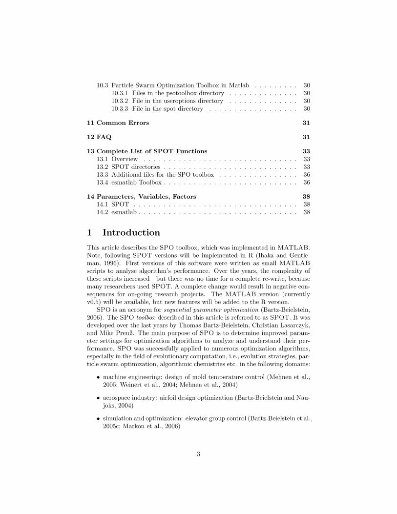
The initial console output from the SPOT run (see Fig. 2) can be explained asfollows. First, all files from previous runs are deleted to ensure a clean start(line 2-8). After that, the user defined region of interest for the (two) factorsto be optimized are diplayed (line 9,10). The initial design consists of 16 pointswithin the specified regions. The design points are displayed in line 11-26.
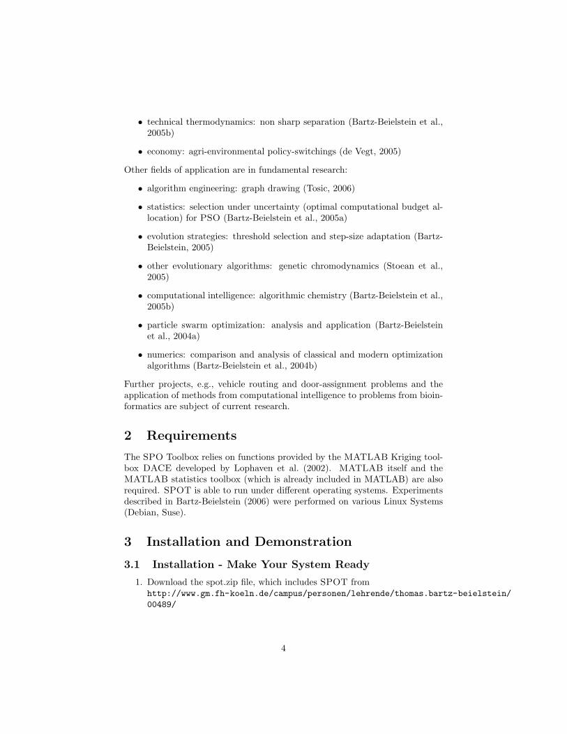
The last lines from the console output read as shown in Fig. 3. Line 4 showsthe factor settings from the best configuration and the corresponding functionvalues.
3.2.3 SPO Plots
Figure 4 shows results from the run demo1000.
4 How SPO works
The SPO can determinate and improve parameter settings for any extern algo-rithm, which could be written in any programming language. The communica-tion between SPO and the extern algorithm is transacted via simple structuredtext files. To make your algorithm able to interact with SPO it is necessary
6
1: >> spotdriver(’demo1000’)
2: Clean up finished.
3: spot/demo1000.des deleted.
4: spot/demo1000.bst deleted.
5: spot/demo1000.res deleted.
6: spot/demo1000.dac deleted.
7: spot/demo1000.bcl deleted.
8: spot/demo1000.fbs deleted.
9: 1 50
10: 2 10
11: 25.347 5.2225
12: 44.583 2.9659
13: 15.108 3.233
14: 26.988 4.2093
15: 34.355 2.4231
16: 43.146 6.2626
17: 29.96 8.1013
18: 37.807 4.8361
19: 18.828 7.9191
20: 8.4869 9.5098
21: 36.572 3.8406
22: 49.363 5.6897
23: 22.198 9.4159
24: 12.448 7.2514
25: 4.6023 6.8547
26: 2.2425 8.7144
27: Initial designs written: Initialization done.................
Figure 2: SPOT generated output.
1: --- SPO step 7 of Inf. ---Algorithm runs: 63 of 50 ---
2: ’NPARENTS’ ’NU’
3: 2 8.7144
4: Min: 9.60936e-07, MinMerged: 4.81543e-05
5: Theta values: 0.5946 2.181
Figure 3: SPOT generated output. Final values.
7

Figure 4: left: predicted function values; right: mean squared error
Figure 5: Effect plots
5. USER
ALGORITHM(e.g. cmaes.m)
1. SPO 8. Output(plots and textoutput)
2. CONFIG(e.g. demo1000.m)
3. ROI(e.g. demo1000.roi)
6. CONFIG(e.g. cmaesdemo1000.m)
USER-side
SPO-side(SPO/USER interface)7. RES
(e.g. demo1000.res)
3. DES
(e.g. demo1000.des)
shell(e.g. cmaesspot.m)
Figure 6: Functional principle of the SPO Toolbox
8
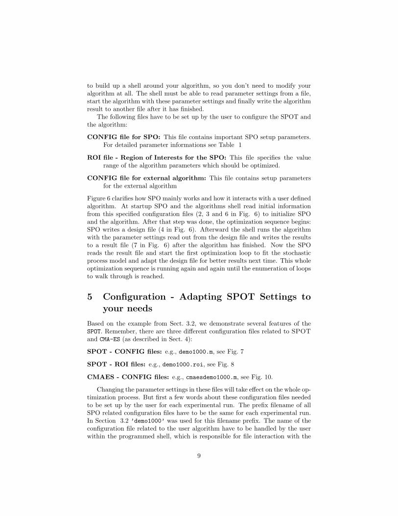
to build up a shell around your algorithm, so you don’t need to modify youralgorithm at all. The shell must be able to read parameter settings from a file,start the algorithm with these parameter settings and finally write the algorithmresult to another file after it has finished.
The following files have to be set up by the user to configure the SPOT andthe algorithm:
CONFIG file for SPO: This file contains important SPO setup parameters.For detailed parameter informations see Table 1
ROI file - Region of Interests for the SPO: This file specifies the valuerange of the algorithm parameters which should be optimized.
CONFIG file for external algorithm: This file contains setup parametersfor the external algorithm
Figure 6 clarifies how SPO mainly works and how it interacts with a user definedalgorithm. At startup SPO and the algorithms shell read initial informationfrom this specified configuration files (2, 3 and 6 in Fig. 6) to initialize SPOand the algorithm. After that step was done, the optimization sequence begins:SPO writes a design file (4 in Fig. 6). Afterward the shell runs the algorithmwith the parameter settings read out from the design file and writes the resultsto a result file (7 in Fig. 6) after the algorithm has finished. Now the SPOreads the result file and start the first optimization loop to fit the stochasticprocess model and adapt the design file for better results next time. This wholeoptimization sequence is running again and again until the enumeration of loopsto walk through is reached.
5 Configuration - Adapting SPOT Settings toyour needs
Based on the example from Sect. 3.2, we demonstrate several features of theSPOT. Remember, there are three different configuration files related to SPOTand CMA-ES (as described in Sect. 4):
SPOT - CONFIG files: e.g., demo1000.m, see Fig. 7
SPOT - ROI files: e.g., demo1000.roi, see Fig. 8
CMAES - CONFIG files: e.g., cmaesdemo1000.m, see Fig. 10.
Changing the parameter settings in these files will take effect on the whole op-timization process. But first a few words about these configuration files neededto be set up by the user for each experimental run. The prefix filename of allSPO related configuration files have to be the same for each experimental run.In Section 3.2 ’demo1000’ was used for this filename prefix. The name of theconfiguration file related to the user algorithm have to be handled by the userwithin the programmed shell, which is responsible for file interaction with the
9

algorithmname= ’cmaesspot’;
algorithmcfgname=’cmaesdemo1000’;
budget=50;
dacemodelname=’’;
defaulttheta=1;
designtype = ’lhd’;
doecenterpoints = 4;
isotropic=0;
lhdintervals=0;
lhdsamples= 16;
loval=1E-3;
maxsamples = 10000;
maxsteps=Inf;
maxrepeats=50;
mergetype=2;
meta = 0;
na=40;
new=1;
newdesignsize=2;
npoints=10;
ntestpointsperdim=10000;
repeats=1;
seed=0;
spotdirname=’spot/’;
spotcmodel=’corrgauss’;
%spotpredictor=’tree’;
spotpredictor=’dace’;
spotrmodel=’regpoly0’;
tol=1.e-2;
upval=100;
verbosity=2;
yname=’Y’;
Figure 7: demo1000.m. Table 1 explains these variables.
name low high isint pretty
NPARENTS 1 50 TRUE ’NPARENTS’
NU 2 10 FALSE ’NU’
Figure 8: demo1000.roi specifies the region of interest for two factors.
10

user algorithm. In section 3.2 the CMAES shell uses ’cmaesdemo1000’ for file-name prefix. The interface files demo1000.des and demo1000.res are generatedautomatically by SPO.
5.1 Modifying the ’Region Of Interest’
The ROI (region of interest) file contains the interesting value ranges of thealgorithm parameters that should be optimized. These ranges are specified bytwo design points each (high and low limit value). The content of the ROI fileused in the example from section 3.2 is shown in figure 8. The file structure iscomparable with an array which elements are separated by blanks. First line actsas a headline for the specified regions of interest which are listed below. Eachremaining line contains ROI information for one parameter to be optimized.The values, that have to be set up for each parameter are explained below:
1. name - factor name to be tuned
2. low - specifies the lower limit value for this factor
3. high - specifies the upper limit value for this factor
4. isint - exclusive use of integer for values of this factor? (could be TRUEor FALSE)
5. pretty - pretty print variant of the factor name, e.g., for axes labeling
The regions of interest can be modified to have a look on the performancewith other parameter value ranges. To adjust the regions of interest, the ROIfile can be modified using a simple text editor, or Matlab’s editor. This changeis related to the SPO (and not to the user’s algorithm), therefore changes areperformed in the file demo1000.m. Our general philosophy is to generate repro-ducible results. This can be achieved by assigning each experimental setup oneunique experiment number. In our first example, we started with demo1000.Thus, the next experiment will be demo1001. This experiment requires thefollowing files:
demo1001.m: SPOT related setup
demo1001.roi: Names and regions of interest of the factors to be tuned
cmaesdemo1001.m: Setup of the user defined optimization algorithm. Weuse cmaes.m and add the prefix cmaes to the names of the configurationfiles.
Change the ROI file content like shown in figure 9 and run SPOT by calling
>> spotdriver(’demo1001’)
to see how it affects the SPO result.
11

name low high isint prettyNPARENTS 1 10 TRUE ’NPARENTS’NU 2 20 FALSE ’NU’
Figure 9: Region of interest file demo1001.roi
%Algorithm design:nparents = 1;nu = 1;%Problem design:fname = ’fsphere’;tmax = 1000;startpoint = 10;lb = 10;ub = 100;stepinit = ’detmod’;delta = 0;dim = 10;% Technical stuffuserdirname=pwd;%%The following parameters might be useful for future releases:%init = ’nunirnd’;termcriteria = ’iterations’;noisetype = ’noNoise’;noisedistribution = ’noNoise’;noiselevel = 0;testset = ’gert’;gm = 0;xopt = 0;successlimit = 0.01;showrun = 0;showpoints = 0;showendpoints = 0;showsuccessfullstartpoints = 0;showunsuccessfullstartpoints = 0;interval = 0;intervalsize = 100;
Figure 10: cmaesdemo1000.m
12

Table 1: detailed information about parameters in SPOT Configuration files(e.g. demo1000.m)algorithmname Call to the algorithm to be tuned. A script or batch file that calls
the optimization algorithm has to be specified here, e.g., ’cmaesspot’algorithmcfgname Configurationfile used by the algorithm to be tuned, e.g., ’cmaes-
demo1000’budget Maximum number of runs of the heuristic. Can be set to “Inf” if
other termination criteria should be used.defaulttheta Only for spotpredictor = ’dace’: Default theta values in the
DACE modeldesigntype Set this to “lhd” in order to use space filling (Latin hypercube de-
signs) or to “doe” to use classical desing of experiments.doecenterpoints Only for spotpredictor = ’doe’: Number of center points for the
DOEisotropic Define number of theta values, default is # of factors, which defines
anisotropic models. Set nTheta to 1 to use isotropic models.lhdintervals Lower and upper bound for the LHS. Used for the ROI.lhdsamples Number of initial configurations (initial sample size) of the heuristic
to be performed.loval Only for spotpredictor = ’dace’: lower bound for theta values in
the DACE modelmaxrepeats Maximum number of repeats for one algorithm parameter setting.
“Inf” if other termination criteria should be used. See also: budget,
maxsteps.maxsamples Maximum number of sample points used in the prediction.maxsteps Maximum number of runs of the SPO. Can be set to “Inf” if other
termination criteria should be used. See also: budget, maxrepeats.mergetype Determines how results from one run configuration should be aggre-
gated.Can be one of the following: “1”: mean, “2”: medianmeta Set this value to “1” if meta runs should be performed, see Sect. 8.
Otherwise choose “0” (default).na Only for spotpredictor = ’dace’ or if a dacemodel is plotted: Grid
size for the dace model plot. Default “40”.new To start a new run, especially with filenames that have been used
for other runs and these files should be overwritten, set this valueto ”1”. To continue an existing experiment, choose ”0”.
newdesignsize Number of algorithm configurations to be evaluated by the algo-rithm (should be small). Default “2”.
npoints number of points for effect plotsnsteps Number of sequential optimization steps to be performed.ntestpointsperdim Number of testpoints (huge!) genereted by the predictor.repeats Number of repeats in the inital design. Default “1”.seed Initial seed for the SPOT functions. Default “0”.spotcmodel Only for spotpredictor = ’dace’: correlation model in the DACE
modelspotdirname Directory where the optimization algorithm reads configuration and
writes results files (use a closing \ or /). Default: Directory wherethe spot files reside.
spotpredictor Specifcy the SPOT predictor: “dace” uses Kriging (slow, but exact),“tree” uses regression trees (fast, can handle categorical factors aswell)
spotrmodel Only for spotpredictor = ’dace’: regression model in the DACEmodel
tol tolerance for effect plotsupval Only for spotpredictor = ’dace’: upper bound for theta values in
the DACE modelyname name of the value to be optimized (minimization). Default “Y”.
Will be written in the res and desfiles.
13

Table 2: detailed information about parameters in CMAES Configuration file(e.g. cmaesdemo1000.m)userdirname Path to the *des and *res-files
5.2 Modifying the SPO configuration
5.2.1 Changing the predictor
The predictions used in the demo1000 setup are based on the DACE model.Other models, e.g., classical regression or tree based models can be used, too.Next, we discuss how to use a tree-based regression model. Again, this changeis related to the SPO (and not to the user’s algorithm), therefore changes areperformed in the file demo1001.m. Our general philosophy is to generate repro-ducible results. This can be achieved by assigning each experimental setup oneunique experiment number. In our previous example, we used demo1001. Thus,the next experiment will be demo1002. This experiment requires the followingfiles:
demo1002.m: SPOT related setup
demo1002.roi: Names and regions of interest of the factors to be tuned
cmaesdemo1002.m: Setup of the user defined optimization algorithm. Weuse cmaes.m and add the prefix cmaes to the names of the configurationfiles.
5.3 Modifying the CMAES configuration
5.3.1 Modifying the Problem Dimension
The experimenter might be interested in the question if similar algorithm designsare beneficial for different problem dimensions. Therefore, he has to modify theproblem design. The problem design subsumes information about the objectivefunction, e.g., the problem dimension, and specifies the available budget, e.g.,time, number of function evaluations etc. To modify the problem dimension,the file cmaesdemo1000.m (Fig. 10) has to be edited. For example, using a texteditor, you can change dim = 10 to dim =100 to analyze a 100 dimensionalproblem.
5.3.2 Modifying Factors that Remain Constant (Algorithm Design)
Factors that are varied during the sequential parameter optimization are speci-fied in the ROI file. Many algorithms have factors that remain constant duringthe sequential parameter optimization. They are specified in the cmaesdemo1000.mfile. By default, every factor of the optimization algorithm is specified in thecmaesdemo1000.m file and SPO overwrites these values with values generatedin the ROI file.
14

5.3.3 The file getuseroptions.m
The file getuseroptions.m can be found in the subdirectory useroptions.Users can specify default factor settings and some rather technical informationssuch as directory names. It has to be modified if new factors are added to thealgorithm design as explained in Sect. 5.4
5.4 Adding Factors to the Algorithm Design
5.4.1 Overview
In this section we consider how new factors can be added to the algorithmdesign. The example presented in section 5 uses two factors: NPARENTS and NU.The related experiment will be referred to as demo1002. The following files haveto be modified to include a new factor:
cmaes.m: Since CMA-ES does not provide an interface for factors, we haveto change the source code of cmaes.m. This is against our philosophy,because we usually do not change the source code. Future releases of theCMA-ES might provide an interface.
cmaesspot.m: Here we add the additional factor which is passed to cmaes.m.
getuseroptions.m: This function has to be modified, because it assigns a de-fault value to the new factor.
cmaesgenerateresfile.m: This function writes results from the CMA-ES runs.Here we have to add the new factor, too.
demo1002.roi: Here we specify the additional region of interest for the newfactor.
demo1002.m: Here we specify the settings (number of algorithm runs, predic-tor, etc.) of the SPO.
5.4.2 The new Factor: CS (TCCS)
We consider the time constant for cumulation for step-size control (tccs ∈]0, 1]).Since cs is already used by MATLAB, we changed the variable name from csto tccs in the cmaes.m file (Hansen and Ostermeier, 2001). Unfortunately,CMA-ES does not provide an interface for this factor. Therefore, we added thefollowing lines to the cmaes.m source code:
defopts.tccs = ’0.5 % time constant for cumulation for step-size control’;
...
%qqq hacking of a different parameter setting, e.g. for ccov or damps,
% can be done here.
% ccov = 0.0*ccov; disp([’CAVE: ccov=’ num2str(ccov)]);
%TBB (Feb, 12th 2008):
tccs = opts.tccs;
15

Now we can use the opts structure to handle the tccs parameter. Modificationsof the cmaes.m file are documented in the source code.
The next file we have to consider is cmaesspot.m. Here we add the lines
tccs = spotgetdesignvalues(a, b, ’TCCS’);
...
if ismember(’TCCS’, b)
useroptions.ad.tccs = tccs(i);
opts.tccs = tccs(i);
end;
Since cmaesspot.m calls getuseroptions.m, we have to modify this func-tion, too. We have to add one line to the algorithm design:
’ad’, struct(... % algorithm design from Table 6.3 in [Bart06a, p.97]
’designfactorname1’, ’’,... %factors to be tuned
’nparents’, nparents, ... % population size [cmaes]
’tccs’, tccs, ... % time constant for cumulation for step-size control
’designfactornamen’, ’’), ... %n-th factor to be tuned
...
The new factor can be read by the CMA-ES, but it not written to the result-file. Therefore we modifify the function cmaesgenerateresfile.m as follows:
function cmaesgenerateresfile(options)
a = exist(options.file.resfilename,’file’);
if (a == 0)
fid = fopen(options.file.resfilename,’w’);
fprintf(fid,’%s %s %s %s %s %s %s %s %s %s %s %s %s %s’,...
’Y’,’SUCC’,’NPARENTS’,’NU’,’TCCS’,’FNAME’,’ITER’,...
’DIM’,...
’CONFIG’,’SEED’);
fclose(fid);
end
fid = fopen(options.file.resfilename,’a’);
fprintf(fid,’\n%g %d %d %g %g %s %d %d %d %d’,...
options.obj.y,...
options.obj.succ, ...
options.ad.nparents,...
options.ad.nu,...
options.ad.tccs,...
options.pd.fname, ...
options.pd.tmax,...
options.pd.dim,...
options.vars.configurationnumber,...
options.obj.thisseed);
fclose(fid);
And, we have to set up the region of interest in the demo1002.roi file forthis factor:
name low high isint pretty
NPARENTS 1 50 TRUE ’NPARENTS’
NU 2 10 FALSE ’NU’
TCCS 0 1 FALSE ’TCCS’
Finally, we have to specify the file for the SPO demo1002.m (here we simplycopy the file demo1000.m, and add the following line to the file demo1000.mwhich will be save as tt demo1002.m):
16
0 20 40−10
0
10
20
30
NPARENTS
Fun
ctio
n va
lue
Y
0 5 10−5
0
5
10
15
NU
Fun
ctio
n va
lue
Y
−0.5 0 0.5 1 1.5−5
0
5
10
15
TCCS
Fun
ctio
n va
lue
Y
010
2030
4050
24
68
10−10
0
10
20
30
40
NPARENTSNU
Fun
ctio
n va
lue
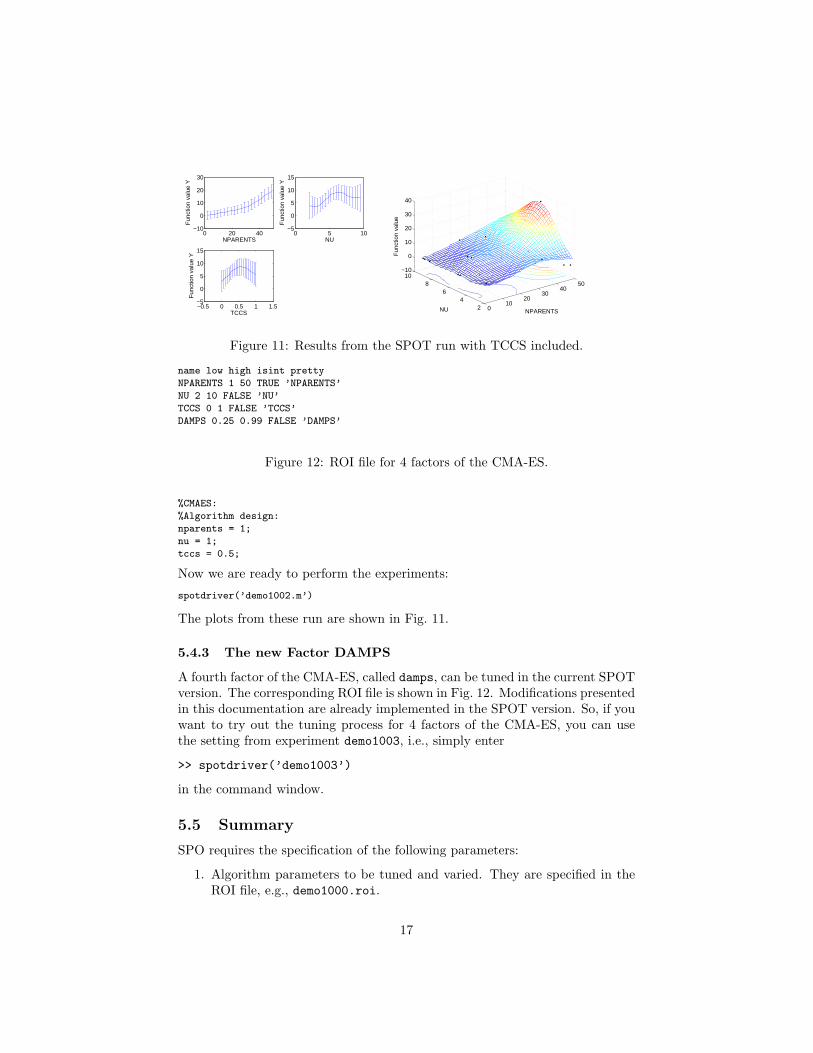
Figure 11: Results from the SPOT run with TCCS included.
name low high isint pretty
NPARENTS 1 50 TRUE ’NPARENTS’
NU 2 10 FALSE ’NU’
TCCS 0 1 FALSE ’TCCS’
DAMPS 0.25 0.99 FALSE ’DAMPS’
Figure 12: ROI file for 4 factors of the CMA-ES.
%CMAES:
%Algorithm design:
nparents = 1;
nu = 1;
tccs = 0.5;
Now we are ready to perform the experiments:
spotdriver(’demo1002.m’)
The plots from these run are shown in Fig. 11.
5.4.3 The new Factor DAMPS
A fourth factor of the CMA-ES, called damps, can be tuned in the current SPOTversion. The corresponding ROI file is shown in Fig. 12. Modifications presentedin this documentation are already implemented in the SPOT version. So, if youwant to try out the tuning process for 4 factors of the CMA-ES, you can usethe setting from experiment demo1003, i.e., simply enter
>> spotdriver(’demo1003’)
in the command window.
5.5 Summary
SPO requires the specification of the following parameters:
1. Algorithm parameters to be tuned and varied. They are specified in theROI file, e.g., demo1000.roi.
17

2. SPOT specific parameters, e.g., (demo1000.m)
In addition, the algorithm which should be tuned requires the specification ofthe following parameters:
1. Algorithm parameters that remain constant
2. Problem specific parameters
In our example (cmaesdemo1000.m) was used to specify these parameters.
6 Implementing Interfaces for the CMA-ES
6.1 Overview
In the following section, details of the SPOT implementation will be explained.We present examples, how SPOT can be adapted to your needs. This sectionwill present some guidelines so that SPOT can be used for new algorithms.
6.2 The SPOT interface to the CMAES program
cmaes.m should be able to read SPO design files and write SPO resfiles. There-fore we write a MATLAB function called cmaesspot.m.
6.2.1 cmaesspot.m
function cmaesspot(filename)
clear useroptions;
useroptions = getuseroptions(filename);
opts.MaxFunEvals=useroptions.pd.tmax;
clear A;
%%%%%%%%%%%%%%%%%%%%%%%%%%%%%%%%%%%%%%%
% 2. Load design file data
[a,b] = autotextread(useroptions.file.desfilename);
CONFIG = (eval(strcat(’a.’,’CONFIG’)));
REPEATS = (eval(strcat(’a.’,’REPEATS’)));
SEED = (eval(strcat(’a.’,’SEED’)));
nofexp = length(CONFIG); %number of experiments
% Assign vectors of algorithm design values:
nparents = spotgetdesignvalues(a, b, ’NPARENTS’);
nu = spotgetdesignvalues(a, b, ’NU’);
%
for i=1:nofexp
useroptions.vars.numberofruns = REPEATS(i);
for j=1:REPEATS(i) %each experimental setting is repeated REPEAT(i) times
useroptions.vars.repeatcounter = j;
%opts=cmaes;
opts.StopFitness=1e-10;
% Overwrite default values with algorithm design values.
if ismember(’NPARENTS’, b)
useroptions.ad.nparents = round(nparents(i));
18

opts.ParentNumber = useroptions.ad.nparents;
end;
if ismember(’NU’, b)
useroptions.ad.nu = nu(i);
opts.PopSize = round(nparents(i)*nu(i));
end;
% Run specific settings:
useroptions.vars.configurationnumber = CONFIG(i);
% SEED
useroptions.obj.thisseed = SEED(i)+j;
% the following is performed in cmaes.m:
%rand(’state’,useroptions.obj.thisseed);
%randn(’state’,useroptions.obj.thisseed);
opts.Seed = useroptions.obj.thisseed;
% Start one CMAES run:
opts.Display = ’off’; opts.Plotting = ’off’;
opts.VerboseModulo = 0;
%objectivefunctionhandle = str2func();
[XMIN, FMIN, COUNTEVAL, STOPFLAG, OUT, BESTEVER]=cmaes(useroptions.pd.fname,5*ones(10,1), 1.5, opts);
useroptions.obj.y = FMIN;
fprintf(’.’);
cmaesgenerateresfile(useroptions);
% End of one CMA-ES run
end
end
We recommend the adaption of the function getuseroptions.m, which specifiesa generic options structure.
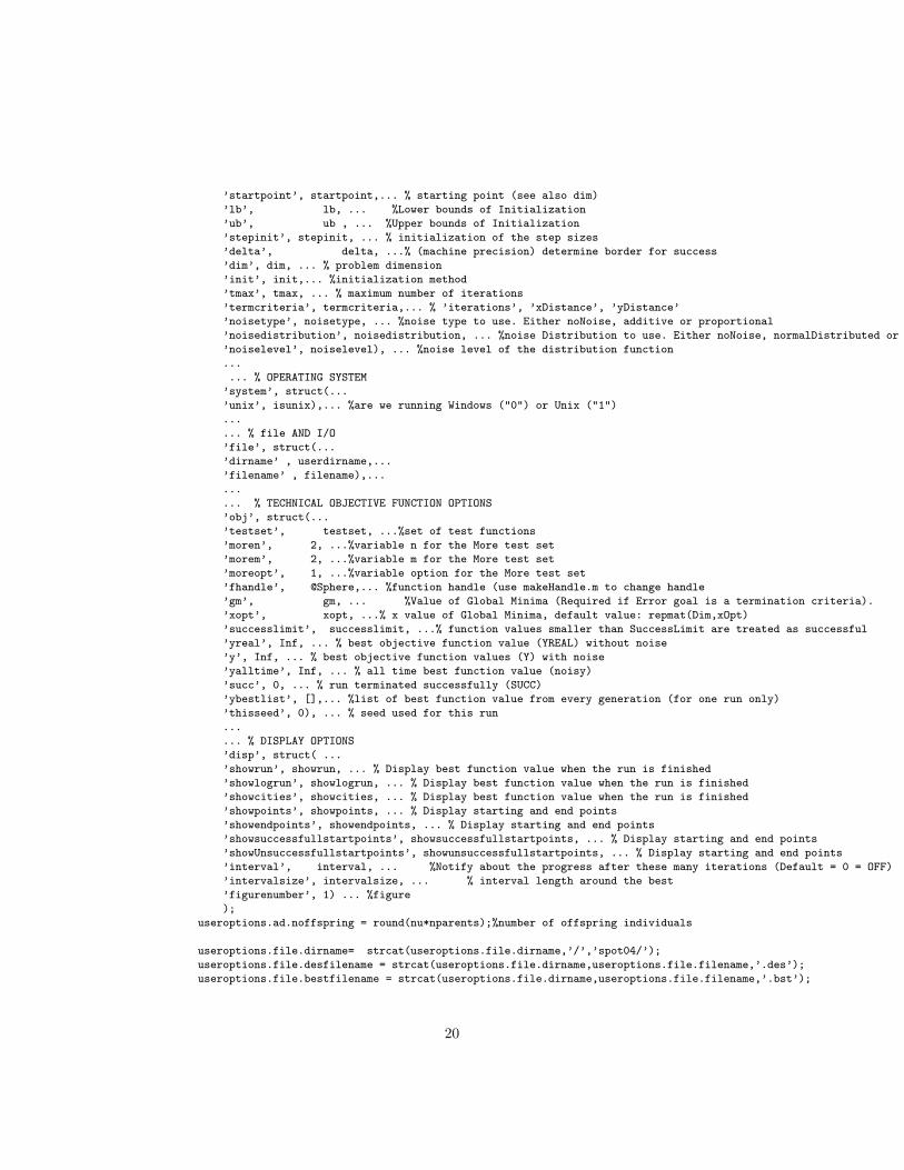
6.2.2 getuseroptions.m
The function getuseroptions calls the function cmaesdemo1000.m which spec-ifies the default settings for the algorithm and problem design. Based on thesevalues, getuseroptions generates the structure useroptions, which is usedduring the optimization runs.
function useroptions = getuseroptions(filename)
userprefix = ’cmaes’;
userfhandle = str2func(strcat(userprefix,filename)); % add es specific prefix for the configuration file
userfhandle();
useroptions = struct(...
...
... % ALGORITHM DESIGN
’ad’, struct(... % algorithm design from Table 6.3 in [Bart06a, p.97]
’designfactorname1’, ’’,... %factors to be tuned
’nparents’, nparents, ... % population size [cmaes]
’designfactornamen’, ’’), ... %n-th factor to be tuned
...
... % PROBLEM DESIGN
’pd’, struct(...
’fname’, fname, ... % objective function
19
’startpoint’, startpoint,... % starting point (see also dim)
’lb’, lb, ... %Lower bounds of Initialization
’ub’, ub , ... %Upper bounds of Initialization
’stepinit’, stepinit, ... % initialization of the step sizes
’delta’, delta, ...% (machine precision) determine border for success
’dim’, dim, ... % problem dimension
’init’, init,... %initialization method
’tmax’, tmax, ... % maximum number of iterations
’termcriteria’, termcriteria,... % ’iterations’, ’xDistance’, ’yDistance’
’noisetype’, noisetype, ... %noise type to use. Either noNoise, additive or proportional
’noisedistribution’, noisedistribution, ... %noise Distribution to use. Either noNoise, normalDistributed or uniformDistributed
’noiselevel’, noiselevel), ... %noise level of the distribution function
...
... % OPERATING SYSTEM
’system’, struct(...
’unix’, isunix),... %are we running Windows ("0") or Unix ("1")
...
... % file AND I/O
’file’, struct(...
’dirname’ , userdirname,...
’filename’ , filename),...
...
... % TECHNICAL OBJECTIVE FUNCTION OPTIONS
’obj’, struct(...
’testset’, testset, ...%set of test functions
’moren’, 2, ...%variable n for the More test set
’morem’, 2, ...%variable m for the More test set
’moreopt’, 1, ...%variable option for the More test set
’fhandle’, @Sphere,... %function handle (use makeHandle.m to change handle
’gm’, gm, ... %Value of Global Minima (Required if Error goal is a termination criteria).
’xopt’, xopt, ...% x value of Global Minima, default value: repmat(Dim,xOpt)
’successlimit’, successlimit, ...% function values smaller than SuccessLimit are treated as successful
’yreal’, Inf, ... % best objective function value (YREAL) without noise
’y’, Inf, ... % best objective function values (Y) with noise
’yalltime’, Inf, ... % all time best function value (noisy)
’succ’, 0, ... % run terminated successfully (SUCC)
’ybestlist’, [],... %list of best function value from every generation (for one run only)
’thisseed’, 0), ... % seed used for this run
...
... % DISPLAY OPTIONS
’disp’, struct( ...
’showrun’, showrun, ... % Display best function value when the run is finished
’showlogrun’, showlogrun, ... % Display best function value when the run is finished
’showcities’, showcities, ... % Display best function value when the run is finished
’showpoints’, showpoints, ... % Display starting and end points
’showendpoints’, showendpoints, ... % Display starting and end points
’showsuccessfullstartpoints’, showsuccessfullstartpoints, ... % Display starting and end points
’showUnsuccessfullstartpoints’, showunsuccessfullstartpoints, ... % Display starting and end points
’interval’, interval, ... %Notify about the progress after these many iterations (Default = 0 = OFF)
’intervalsize’, intervalsize, ... % interval length around the best
’figurenumber’, 1) ... %figure
);
useroptions.ad.noffspring = round(nu*nparents);%number of offspring individuals
useroptions.file.dirname= strcat(useroptions.file.dirname,’/’,’spot04/’);
useroptions.file.desfilename = strcat(useroptions.file.dirname,useroptions.file.filename,’.des’);
useroptions.file.bestfilename = strcat(useroptions.file.dirname,useroptions.file.filename,’.bst’);
20

useroptions.file.resfilename = strcat(useroptions.file.dirname,useroptions.file.filename,’.res’) ;
useroptions.file.dacemodelname = strcat(useroptions.file.dirname,useroptions.file.filename,’.dac’);
useroptions.file.bestconfiglistname = strcat(useroptions.file.dirname,useroptions.file.filename,’.bcl’);
useroptions.file.xbestfilename = strcat(useroptions.file.dirname,useroptions.file.filename,’.xbst’);
useroptions.file.finalbestfilename = strcat(useroptions.file.dirname,useroptions.file.filename,’.fbs’);
useroptions.obj.ffandle = spotmakehandle(useroptions.pd.fname);
useroptions.pd.startpoint = useroptions.pd.startpoint * ones(1,useroptions.pd.dim);
6.2.3 cmaesdemo1000.m
The file cmaesdemo1000.m is a classical configuration file. It defines the settingsfor the algorithm and problem design. For example, if you want to change theproblem dimension, you do not have to change the MATLAB code, but thesettings in this configuration file.
%CMAES:
%Algorithm design:
nparents = 1;
nu = 1;
%Problem design:
fname = ’fsphere’;
tmax = 1000;
startpoint = 10;
lb = 10;
ub = 100;
stepinit = ’detmod’;
delta = 0;
dim = 100;
% Technical stuff
userdirname=pwd;
%
%The following parameters might be useful for future releases:
%
init = ’nunirnd’;
termcriteria = ’iterations’;
noisetype = ’noNoise’;
noisedistribution = ’noNoise’;
noiselevel = 0;
testset = ’gert’;
gm = 0;
xopt = 0;
successlimit = 0.01;
showrun = 0;
showpoints = 0;
showendpoints = 0;
showsuccessfullstartpoints = 0;
showunsuccessfullstartpoints = 0;
interval = 0;
intervalsize = 100;
%
mutation = ’standard’;
cities = ’loadst70’;
showlogrun = 0;
showcities = 0;
21

6.2.4 cmaesgenerateresfile
The cmaesspot.m function calls the function cmaesgenerateresfile.m to writedata in the resfile format.
function cmaesgenerateresfile(options)
a = exist(options.file.resfilename,’file’);
if (a == 0)
fid = fopen(options.file.resfilename,’w’);
fprintf(fid,’%s %s %s %s %s %s %s %s %s %s %s %s %s’,...
’Y’,’SUCC’,’NPARENTS’,’NU’,’FNAME’,’ITER’,...
’DIM’,...
’CONFIG’,’SEED’);
fclose(fid);
end
fid = fopen(options.file.resfilename,’a’);
fprintf(fid,’\n%g %d %d %g %s %d %d %d %d’,...
options.obj.y,...
options.obj.succ, ...
options.ad.nparents,...
options.ad.nu,...
options.pd.fname, ...
options.pd.tmax,...
options.pd.dim,...
options.vars.configurationnumber,...
options.obj.thisseed);
fclose(fid);
6.2.5 The Objective Function
For this demo, we have chosen the following objective function: fsphere.mwhich is located in the directory objectivefunctions.
function f=fsphere(x)f=sum(x.^2, 1);
6.2.6 The Design File
Each line in the design file contains one run configuration. Note, each configura-tion can be repeated several times (with different seeds). Configuration 1 fromthe file demo1000.des is repeated twice, whereas configuration 2 is repeatedonly once:
NPARENTS NU REPEATS CONFIG SEED STEP2 2 2 1 123 17 4 1 2 123 1
6.2.7 Testing the Interface
Now we are ready for testing the interface. We can call the cmaesspot.m func-tion as follows:
cmaesspot(’demo1000’)
22
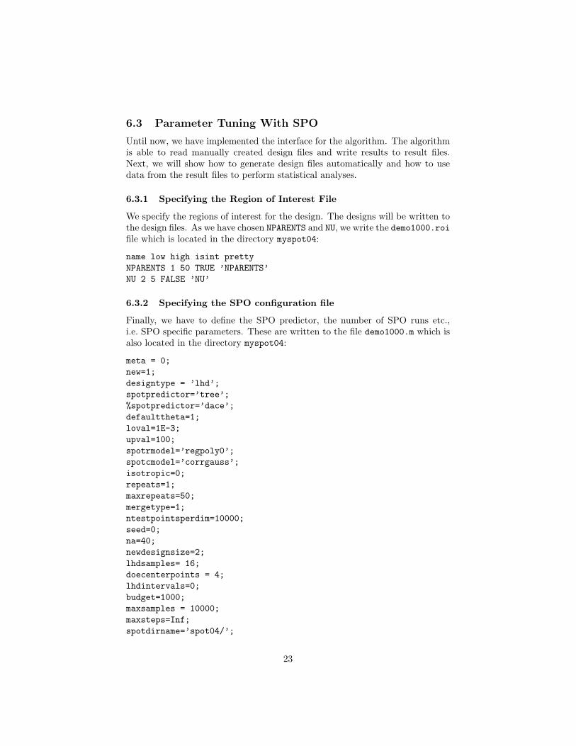
6.3 Parameter Tuning With SPO
Until now, we have implemented the interface for the algorithm. The algorithmis able to read manually created design files and write results to result files.Next, we will show how to generate design files automatically and how to usedata from the result files to perform statistical analyses.
6.3.1 Specifying the Region of Interest File
We specify the regions of interest for the design. The designs will be written tothe design files. As we have chosen NPARENTS and NU, we write the demo1000.roifile which is located in the directory myspot04:
name low high isint prettyNPARENTS 1 50 TRUE ’NPARENTS’NU 2 5 FALSE ’NU’
6.3.2 Specifying the SPO configuration file
Finally, we have to define the SPO predictor, the number of SPO runs etc.,i.e. SPO specific parameters. These are written to the file demo1000.m which isalso located in the directory myspot04:
meta = 0;new=1;designtype = ’lhd’;spotpredictor=’tree’;%spotpredictor=’dace’;defaulttheta=1;loval=1E-3;upval=100;spotrmodel=’regpoly0’;spotcmodel=’corrgauss’;isotropic=0;repeats=1;maxrepeats=50;mergetype=1;ntestpointsperdim=10000;seed=0;na=40;newdesignsize=2;lhdsamples= 16;doecenterpoints = 4;lhdintervals=0;budget=1000;maxsamples = 10000;maxsteps=Inf;spotdirname=’spot04/’;
23

dacemodelname=’’;npoints=10;tol=1.e-2;algorithmname= ’spotga’;yname=’Y’;verbosity=1;
6.3.3 Starting SPOT
We are ready for the SPOT process. It can be called via
spotdriver(’demo1000’)
Please note, that myspot04 has to be chosen as the working directory and allsubdirectories have to be included in the MATLAB path.
Summarizing, the following files are necessary for the SPOT, where xxxdenotes the experiment name, e.g. demo1000:
xxx.roi: Region of interest.
xxx.m: SPOT configuration file.
cmaesxxx.m: CMA-ES configuration file. Optimization problem configura-tion.
cmaesspot.m: Interface to the cmaes.m algorithm. Read design file.
getuseroptions.m: Read configuration from the cmaesxxx.m file and generatethe options structure.
cmaesgenerateresfile.m: Generate the result file.
7 Documentation of SPOT Interfaces
The SPOT concept is very simple and can be used for any optimization algo-rithm that can read and write ASCII files.
SPOT proposes algorithm designs for the algorithm. The algorithm is runwith these designs, results from these runs are written to result files (res-files).SPOT reads the res-files and builds a stochastic process model. Based on thismodel, new algorithm design points are generated and written to the design file(des-file). See also Bartz-Beielstein et al. (2005b).
7.1 Design Files
Design files are ASCII files which store information columnwise. They consist oftwo parts: Header and body. The first line of a design file, the header, describesthe variable names. Entries are separated by blanks. Each of the following linescontains information from one algorithm run. A minimum design file has twolines. It might contain the following information:
24

A REPEATS CONFIG SEED2 3 1 123
“A” denotes the name of algorithm parameter to be tuned, e.g., NPARENTS.Each run is repeated three times with different random seeds, the first run usesseed 123. This is configuration 1.
Based on the values from the des-file the optimization algorithm is run. Itsresults are written to the res-file.
The header has to be the first line while the order of the other lines (rows) isarbitrary. The order of the columns is arbitrary, too. The example from abovecould be written as:
REPEATS CONFIG SEED A3 1 123 2
7.2 Result Files
The structure of result files is the same as for design files: They are des-files withone additional column which contains the result from the optimization runs. Aminimum result file contains the following information:
Y A REPEATS CONFIG SEED0.2 2 3 1 123
This might be one result from an experiment which is based on the des-file fromabove. The algorithm run yields an function value of Y = 0.2.
Based on the values from the res-file SPOT will fit a stochastic processmodel to predict promising design points.
8 Meta Runs
8.1 A first example
SPOT can be used as a meta algorithm that determines improved parametersettings for several configurations. The user can tune one algorithm for severalproblem instances at once. A typical experiment can tackle the question howto determine improved algorithm designs for problem dimensions 10, 20, 30, . . .100.
function spotmeta(spotfilename)
% A clean start:
close all hidden; rand(’state’,0); randn(’state’,0);
% Read spot related options as a structure from file ’spotfilename.m’:
spotoptions = spotgetoptions(spotfilename);
% Generate generic file names:
spotoptions = spotgeneratefilenames(spotoptions);
% meta loop starts here:
if (spotoptions.vars.meta == 1)
kk = 10:10:1000
25

for i = 1:length(kk)
spotoptions.metavar = kk(i);
%spotmetauseroptions(spotoptions);
spotdriver(spotfilename,kk(i));
end
end
spotmeta.m calls spotdriver.m. spotdriver.m writes additional informa-tion to a meta-log file (META.fbs), where fbs stands for final best solution.
if (spotoptions.vars.meta == 1)
% The meta SPOT loop starts here:
% Since the final best file should not be deleted in the meta loop,
% we modify its filename:
spotoptions.file.finalbestfilename = strcat(spotoptions.file.dirname,’META’,’.fbs’);
end;
The function spotanalyzefbs.m can be used for visualizations of the resultsfrom the meta-runs.
The meta-demo can be started by
>> spotmeta(’demo1004’)
8.2 Meta Latin Hypercube Designs
The function spotdriverlhd can be used for testing various initial LHD samplesizes. It differs from spotdriver, because it modifies the the LHD sample size.This feature is implemented as follows:
function spotdriverlhd(spotfilename,metavar)
spotoptions.design.lhdsamples = metavar;
spotdriverlhd can be called from the meta-function spotmetalhd as fol-lows:
function spotmetalhd(spotfilename)
% A clean start:close all hidden; rand(’state’,0); randn(’state’,0);
% Read spot related options as a structure from file ’spotfilename.m’:spotoptions = spotgetoptions(spotfilename);
% Generate generic file names:spotoptions = spotgeneratefilenames(spotoptions);
% meta loop starts here:if (spotoptions.vars.meta == 1)kk = [10 50 100:100:500]
26

for i = 1:length(kk)spotoptions.metavar = kk(i);%spotmetauseroptions(spotoptions);spotdriverlhd(spotfilename,kk(i));
endend
8.2.1 Example
spotmetalhd(’demo1009’) presents an example which is based on the CMA-ES.
9 Analysis
9.1 Kriging Model from Resulfile
spotplotdacefromresfile.m provides a convenient way to generate a Krigingmodel from an existing resultfile.
Modify the following line in spotplatdacefromresfile.m:
spotoptions.design.factornames = {’NPARENTS’,’NU’,’TCCS’,’DAMPS’};
For demonstration, you can call
>> spotplotdacefromresfile(’demo1003’)
9.2 Sensitivity Analysis
Consider the functional relationsship
Y = f( ~X) (1)
Use spotgetfirstordereffects.m to determine first oder effects.
10 Building an Interface From Scratch
This section explains how to build an SPOT interfaces for existing programs.The example in Sect. 10.1 discusses R-programs. Section 10.2 discusses neuralnetworks written in MATLAB. Section refsec:pso describes the integration ofthe psotoolbox.
10.1 Interface to R-Programs
The program used in this example was written in R. It is located in the directorydmc.
27

10.1.1 Files in the DMC Directory
dummy.r: This file is called dummy.r, because it is a placeholder for any pro-gramm written in R, which requires the definition of input parameters (fac-tors, algorithm design). The factors used by dummy.r are cnk0, cnk1, . . . cnk4,cak0, cak1, . . . cak4, mak and mnk. These are altogether 12 factors whichshould be tuned.
### script dummy.r
### filename = des/resfilename prefix, e.g., run0001 (type: STRING)
filename<-commandArgs()[5]
resfilename<-paste(filename,".res",sep="")
desfilename<-paste(filename,".des",sep="")
x.df<-read.table(desfilename, header = T, row.names = NULL)
attach(x.df)
n<-nrow(x.df) # number of configurations
for (i in 1:n)
{
## one configuration,
for (j in 1:REPEATS[i])
{
## one run
## seed = new seed
thisseed <- SEED[i]+j
set.seed(thisseed)
## the function value is determined. Add your R function here:
Y = CNK0[i] + CNK1[i]+ runif(1)
## The header of the resfile was already written by spot.
Here, only results are added to the resfile:
resultline <- cbind(Y, CNK0[i], CNK1[i], CNK2[i], CNK3[i],
CNK4[i], CAK0[i], CAK1[i], CAK2[i], CAK3[i], CAK4[i],
MNK[i], MAK[i], CONFIG[i], thisseed)
write.table(resultline, file = resfilename, quote=FALSE,
row.names=FALSE,append=TRUE,col.names=FALSE)
}
}
detach(x.df)
startR.sh: Under Linux, we use the following (bash) shell script (the Windowsequivalent is a batch-file) to call the R script.
#!/bin/sh
export R_HOME=‘R RHOME‘
export LD_LIBRARY_PATH=$R_HOME/lib
export filename=$1 #"dummy"
/usr/bin/R --vanilla --slave --args spot/$filename < dmc/dummy.r > outFile.txt
dmcspot.m: We use the following MATLAB function to execute the shellscript startR.sh from MATLAB:
function dmcspot(filename)
dmcgenerateresfile(filename)
argstring = [’dmc/startR.sh ’, filename];
system(argstring)
run0001.m: The name of the algorithm (here:dmcspot) is defined in the SPOTconfiguration file run0001.m, which is located in the directory spot. Thisfile contains all settings related to the SPOT run (budget, predictor, etc.)
28

algorithmname= ’dmcspot’;
budget=50;
dacemodelname=’’;
defaulttheta=1;
designtype = ’lhd’;
doecenterpoints = 4;
isotropic=0;
lhdintervals=0;
lhdsamples= 16;
loval=1E-3;
maxsamples = 10000;
maxsteps=Inf;
maxrepeats=50;
mergetype=2;
meta = 0;
na=40;
new=1;
newdesignsize=2;
npoints=10;
ntestpointsperdim=10000;
repeats=1;
seed=0;
spotdirname=’spot/’;
spotcmodel=’corrgauss’;
%spotpredictor=’tree’;
spotpredictor=’dace’;
spotrmodel=’regpoly0’;
tol=1.e-2;
upval=100;
verbosity=2;
yname=’Y’;
run0001.roi: Finally, we have to define the experimental region. This is donein the roi-file:
name low high isint pretty
CNK0 0 1 FALSE ’CNK0"
CNK1 0 1 FALSE ’CNK1"
CNK2 0 1 FALSE ’CNK2"
CNK3 0 1 FALSE ’CNK3"
CNK4 0 1 FALSE ’CNK4"
CAK0 0 1 FALSE ’CAK0"
CAK1 0 1 FALSE ’CAK1"
CAK2 0 1 FALSE ’CAK2"
CAK3 0 1 FALSE ’CAK3"
CAK4 0 1 FALSE ’CAK4"
MNK 4 15 TRUE ’MNK’
MAK 4 15 TRUE ’MAK’
Now, we can start the algorithm from MATLAB with the following command:
>> spotdriver(’run0001’)
Summary:
1. spotdriver.m reads the roi-file (and run0001.m for the SPOT configura-tion). It calls dmcspot.m
29

2. dmcspot.m calls the shell script startR.sh
3. startR.sh calls the R script dummy.r
4. dummy.r reads the desfile and writes results to the resfile.
10.2 Neural Networks in Matlab
10.2.1 Files in the nn directory
narxtest3.m: This is the core NN program which can be run without SPOT.
nnspot.m: This function provides an interface from NN to SPOT.
nngenerateresfile.m: Write information to the resultfile.
nndemo3000.m: Information about the NN setting.
10.2.2 File in the useroptions directory
getuseroptions.m : Add NN algorithm design variables here.
10.2.3 File in the spot directory
demo3000.m: SPOT settings.
demo3000.roi: Region of interest.
10.3 Particle Swarm Optimization Toolbox in Matlab
10.3.1 Files in the psotoolbox directory
pso.m: This is the core PSO program from the psotoolbox which can be runwithout SPOT.
psospot.m: This function provides an interface from pso.m to SPOT.
psogenerateresfile.m: Write information to the resultfile.
psodemo100000.m: Information about the PSO setting.
10.3.2 File in the useroptions directory
getuseroptions.m : Add PSO algorithm design variables here.
10.3.3 File in the spot directory
demo100000.m: SPOT settings.
demo3000.roi: Region of interest.
30

11 Common Errors
Table 3 lists errors, possible causes, and solutions.
12 FAQ
• Where can I find more information about the DACE toolbox?Check: http://www2.imm.dtu.dk/˜hbn/dace/
• My optimization algorithm was written in JAVA, C, C++,... Can I useSPOT?You can use any language if your algorithm is able to handle des- andres-files.
• Does SPOT run without MATLAB?No.
• My optimization algorithm is written in MATLAB. Is there a genericmethod to read des-files?Yes. Reading des-files from MATLAB can be done as follows.
1. Specify the algorithm design variables from your algorithm, e.g., muand nu:
factornames = {’MU’, ’NU’};
2. Read the des-file:
tdfread(designfilename, ’ ’);
3. Overwrite default values with values from the des-file:
for i=1:length(factornames)A(i)=factornames(i);
endfor i=1:length(eval(A{i})) %number of experiments
for j=1:REPEATS(i) %each experimental setting is% repeated REPEAT(i) times.
% Overwrite default values with algorithm% design values.if ismember(’MU’, A)
mu = MU(i);endif ismember(’NU’, A)
nu = NU(i);end...RUN YOUR ALGORITHM...
31
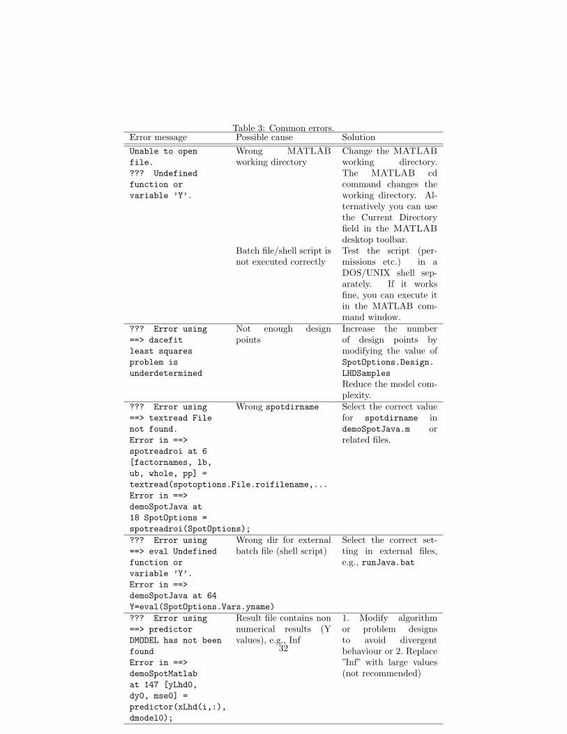
Table 3: Common errors.Error message Possible cause SolutionUnable to openfile.??? Undefinedfunction orvariable ’Y’.
Wrong MATLABworking directory
Change the MATLABworking directory.The MATLAB cdcommand changes theworking directory. Al-ternatively you can usethe Current Directoryfield in the MATLABdesktop toolbar.
Batch file/shell script isnot executed correctly
Test the script (per-missions etc.) in aDOS/UNIX shell sep-arately. If it worksfine, you can execute itin the MATLAB com-mand window.
??? Error using==> dacefitleast squaresproblem isunderdetermined
Not enough designpoints
Increase the numberof design points bymodifying the value ofSpotOptions.Design.LHDSamplesReduce the model com-plexity.
??? Error using==> textread Filenot found.Error in ==>spotreadroi at 6[factornames, lb,ub, whole, pp] =textread(spotoptions.File.roifilename,...Error in ==>demoSpotJava at18 SpotOptions =spotreadroi(SpotOptions);
Wrong spotdirname Select the correct valuefor spotdirname indemoSpotJava.m orrelated files.
??? Error using==> eval Undefinedfunction orvariable ’Y’.Error in ==>demoSpotJava at 64Y=eval(SpotOptions.Vars.yname)
Wrong dir for externalbatch file (shell script)
Select the correct set-ting in external files,e.g., runJava.bat
??? Error using==> predictorDMODEL has not beenfoundError in ==>demoSpotMatlabat 147 [yLhd0,dy0, mse0] =predictor(xLhd(i,:),dmodel0);
Result file contains nonnumerical results (Yvalues), e.g., Inf
1. Modify algorithmor problem designsto avoid divergentbehaviour or 2. Replace”Inf” with large values(not recommended)
32
WRITE RESULT FILEend
end
• How can I evaluate an initial design specified in the ROI file without per-forming any sequential parameter optimization?Set the value maxsteps=0; in the spot configuration file.
• I found a bug in the toolbox.Please report bugs and suggestions for improvement tothomas.bartz-beielstein[at]fh-koeln.de.
• Is there any support available?Currently we cannot provide any support.
• Is SPOT free?Yes.
• Where can I find more information about experimental research, designof experiments (DOE), and design and analysis of computer experiments(DACE)?Bartz-Beielstein (2006) and Santner et al. (2003) are good starting points.
• How can I quote this article?Please mention Bartz-Beielstein et al. (2006) if you have used the SPOtoolbox.
13 Complete List of SPOT Functions
13.1 Overview
Figure 13 illustrates one SPOT run.
13.2 SPOT directories
Files are organized in directories as follows:
core: SPO’s core functions can be found here.
• startspot.m: Helper function to set the path and working directory.
design: Functions to generate experimental designs are placed in this directory.
• spotdoe.m: Generate factorial designs.
• spotlatinhypercube.m: Generate Latin hypercube distributed ran-dom numbers:
– m : number of sample points to generate, if unspecified m = 1.– n : number of dimensions, if unspecified n = m
33

spotdriver(spotfilename)
spotpredictor == 'dace'true
false
spotpredictor == 'tree'true
false
spotoptions.vars.new == 1true
false
delete all results from
previous runs (with same
spotfilename)?
spotcleanup(spotoptions)
delete all files from previous runs (e.g. demo1000.des,
demo1000.res, demo1000.bst, …)
spotwriteinitialdesign(spotoptions)
write the initial design to the specified file
(e.g. demo1000.des)
spotoptions = spotreadroi(spotoptions)
read users roi (region of inteest) file (e.g. demo1000.roi)
and add the roi informations to the spotoptions struct
spotoptions = spotgeneratefilenames(spotoption)
generate all needed filenames (with full path) and add
them to the spotoptions
spotoptions = spotgetoptions(spotfilename)
read all options from the file spotfilename.m (e.g.
demo1000.m) to an struct array named spotoptions
while (~spottermination(spotoptions))if ~((step>maxsteps)||(nalgorithmruns>budget)||(repeats>=maxrepeats))
true
false
do
eval(algorithm)
execute the extern algorithm via the user defined shell
(e.g. eval('cmaesspot('demo1000')'))
[a,b] = autotextread(spotoptions.file.resfilename)
read results from res file (e.g. demo1000.res)
Update configuration number and seed
store the min function value y
generate matrix with algorithm design values
spotwritenewdesign(…)
write new design (.des) file for next run
SPO
Main-Loop
spotplottree(...)
make tree plot output
spotplotresults(…)
make dace plot output
END
verbosity > 1
true
false
make sequential console output
spotpredictor == 'dace'true
false
spotpredictor == 'tree'true
false
[B, dmodel0] = spotpredictdace(...)
create new design points
B = spotpredicttree(...)
create new design points
verbosity > 1
true
false
spotplotprogress(spotoptions)
sequential progress plot output
eleminate double entries
update bst configurationfile and number of repeats
Figure 13: SPOT overview34

Returns S, the generated n dimensional m sample points chosen fromuniform distributions on m subdivions of the interval (0.0, 1.0) Ex-ample: Let a = [1 2 3 4 5 6 7], be the vector of the lower bounds for7 variables, e.g., PSO, and b = [10 20 30 40 50 60 70] the vector ofthe upper bounds. Then latinHypercube(10,7,a,b) generates 10design points.
io: File handling (opening, closing files) functions can be found here.
• spotwritenewdesign.m: Update the design file based on predictionsfrom the DACE or tree model.
• spotwriteinitialdesign.m: Write the initial design.
• spotCleanUp.m: Delete the following files to enable a clean start:
1. des2. bst3. res4. dac5. bcl6. xbst7. fbst
• spotwritedacemodel.m: Write DACE model parameters to a *.dacfile.
• spotreadroi.m: Read the region of interest file.
• spotreadfactornames.m: Returns factornames from res and desfiles.
• spotgetfactornamesfromroi.m: Returns factornames from ROI files.For example, after calling
>> factornames = spotreadfactornamesfromroi(’demo1004.roi’),
factornames{1} returns the name of the first factor and length(factornames)the number of factors
• spotGetOptions.m: Read the SPOT options file.
• spotGenerateFileNames.m: Generate generic file names, i.e.,
1. des2. bst3. res4. dac5. bcl6. xbst7. fbst8. roi
35

meta: Functions to set up and control meta runs can be found here.
• startspot.m: Helper function to set the path and working directory.
predictor: Functions which predict new design points are placed here.
• startspot.m: Helper function to set the path and working directory.
utils: All kind of helper functions are placed in this directory.
• startspot.m: Helper function to set the path and working directory.
• spotMergeData.m: Merge data from several repeats of one run con-figuration. The following merge functions are implemented:
1. mean (1)2. median (2)3. min (3)4. max (4)5. spotbestoutof (4)
This function can also return the standard deviation (0).
visual: • spotploteffectsschonlau.m: Plot one single factor effect. Basedon Schonlau (1997). To be called from spotplotresults.m.
• spotplotresults.m: Call spotploteffectsschonlauf.m for severalfactors. To be called from spotdriver.m.
• spotplotdacemodel.m: Plot the 3 dim DACE model (the first twofactors from the ROI file and the predicted response).
13.3 Additional files for the SPO toolbox
demospotplotresfile.m: Visualize the results from an existing resfile.
spotbestoutof.m: Determines the average from nSamples that have been cre-ated as the minimum from a random sample of size sampleSize. Note:spotbestoutof(x,inf,1) = mean(x), spotbestoutof(x,1,inf) = min(x)
spotgetfirstordereffectsfromresfile.m calculates the first order effectsbased on Saltelli et al. (2008).
spotgetfirstordereffectsfromresfile(’demo1003’)
13.4 esmatlab Toolbox
The esmatlab toolbox contains the following MATLAB functions
addNoise.m: Add noise to the function value.
eseval.m: Enable evaluation of test functions from the More et al. (1981) testset.
36
esInitPopulation: Implement initialization schemes from Bartz-Beielstein(2006, pp. 88) To initialize the set of search points X(0) = {x(0)
1 , . . . , x(0)p },
the following methods can be used:
(DETEQ) Deterministic. Each search point uses the same vector, whichis selected deterministically, i.e., xinit = 1T ∈ Rd. As this methoduses only one starting point xinit, it is not suitable to visualize thestarting points for which the algorithm converged to the optimum.
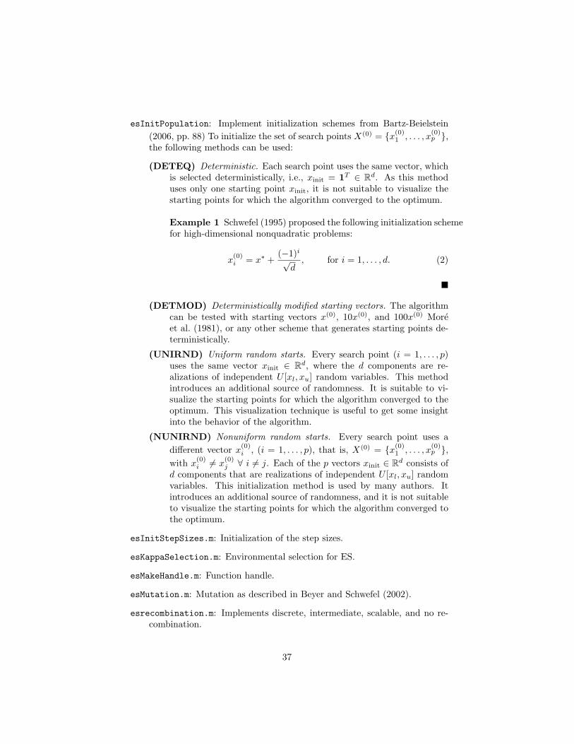
Example 1 Schwefel (1995) proposed the following initialization schemefor high-dimensional nonquadratic problems:
x(0)i = x∗ +
(−1)i
√d
, for i = 1, . . . , d. (2)
�
(DETMOD) Deterministically modified starting vectors. The algorithmcan be tested with starting vectors x(0), 10x(0), and 100x(0) Moreet al. (1981), or any other scheme that generates starting points de-terministically.
(UNIRND) Uniform random starts. Every search point (i = 1, . . . , p)uses the same vector xinit ∈ Rd, where the d components are re-alizations of independent U [xl, xu] random variables. This methodintroduces an additional source of randomness. It is suitable to vi-sualize the starting points for which the algorithm converged to theoptimum. This visualization technique is useful to get some insightinto the behavior of the algorithm.
(NUNIRND) Nonuniform random starts. Every search point uses adifferent vector x
(0)i , (i = 1, . . . , p), that is, X(0) = {x(0)
1 , . . . , x(0)p },
with x(0)i 6= x
(0)j ∀ i 6= j. Each of the p vectors xinit ∈ Rd consists of
d components that are realizations of independent U [xl, xu] randomvariables. This initialization method is used by many authors. Itintroduces an additional source of randomness, and it is not suitableto visualize the starting points for which the algorithm converged tothe optimum.
esInitStepSizes.m: Initialization of the step sizes.
esKappaSelection.m: Environmental selection for ES.
esMakeHandle.m: Function handle.
esMutation.m: Mutation as described in Beyer and Schwefel (2002).
esrecombination.m: Implements discrete, intermediate, scalable, and no re-combination.
37

eswritexbest.m: Write object variables (x values) of the best individual tothe xbest file.
terminate.m: Implement three termination criteria, see Bartz-Beielstein (2006,p.89):
1. budget (number of function evaluations) exhausted2. minimum distance in the objective space reached3. minimum distance to the optimum reached
cmaesdemo1.m: Example ES configuration file. Note, that in our implemen-tation the name of the ES configuration file is generated by adding theprefix ‘es’ to the SPOT configuration file name, i.e., ‘demo1’ results in‘cmaesdemo1’. This is done in getuseroptions.m.
esGetOptions.m: Read options (problem and algorithm designs) from an op-tions file, e.g., cmaesdemo1.m.
generateresfile.m: Write data to the resultfile.
esSpot.m: The ES in MATLAB, i.e., the main class/function/method. It canalso be used as a stand alone ES without the SPOT framework.
14 Parameters, Variables, Factors
This section describes factors and their meaning.
14.1 SPOT
TBD
14.2 esmatlab
lb lower initialization bounds for object variables
ub upper initialization bounds for object variables
References
Bartz-Beielstein, T. (2005). Evolution strategies and threshold selection. InBlesa Aguilera, M. J., Blum, C., Roli, A., and Sampels, M., editors, Proceed-ings Second International Workshop Hybrid Metaheuristics (HM’05), volume3636 of Lecture Notes in Computer Science, pages 104–115, Berlin, Heidel-berg, New York. Springer.
Bartz-Beielstein, T. (2006). Experimental Research in EvolutionaryComputation—The New Experimentalism. Springer, Berlin, Heidelberg, NewYork.
38

Bartz-Beielstein, T., Blum, D., and Branke, J. (2005a). Particle swarm op-timization and sequential sampling in noisy environments. In Hartl, R. andDoerner, K., editors, Proceedings 6th Metaheuristics International Conference(MIC2005), pages 89–94, Vienna, Austria.
Bartz-Beielstein, T., de Vegt, M., Parsopoulos, K. E., and Vrahatis, M. N.(2004a). Designing particle swarm optimization with regression trees. In-terner Bericht des Sonderforschungsbereichs 531 Computational IntelligenceCI–173/04, Universitat Dortmund, Germany.
Bartz-Beielstein, T., Lasarczyk, C., and Preuß, M. (2005b). Sequential param-eter optimization. In McKay, B. et al., editors, Proceedings 2005 Congress onEvolutionary Computation (CEC’05), Edinburgh, Scotland, volume 1, pages773–780, Piscataway NJ. IEEE Press.
Bartz-Beielstein, T., Lasarczyk, C., and Preuß, M. (2006). Sequential parameteroptimization toolbox. Technical Report CI–15x/06, Universitat Dortmund,Germany.
Bartz-Beielstein, T. and Naujoks, B. (2004). Tuning multicriteria evolution-ary algorithms for airfoil design optimization. Interner Bericht des Son-derforschungsbereichs 531 Computational Intelligence CI–159/04, UniversitatDortmund, Germany.
Bartz-Beielstein, T., Parsopoulos, K. E., and Vrahatis, M. N. (2004b). De-sign and analysis of optimization algorithms using computational statis-tics. Applied Numerical Analysis & Computational Mathematics (ANACM),1(2):413–433.
Bartz-Beielstein, T., Preuß, M., and Markon, S. (2005c). Validation and opti-mization of an elevator simulation model with modern search heuristics. InIbaraki, T., Nonobe, K., and Yagiura, M., editors, Metaheuristics: Progressas Real Problem Solvers, Operations Research/Computer Science Interfaces,pages 109–128. Springer, Berlin, Heidelberg, New York.
Beyer, H.-G. and Schwefel, H.-P. (2002). Evolution strategies—A comprehensiveintroduction. Natural Computing, 1:3–52.
de Vegt, M. (2005). Einfluss verschiedener Parametrisierungen auf die Dy-namik des Partikel-Schwarm-Verfahrens: Eine empirische Analyse. InternerBericht der Systems Analysis Research Group SYS–3/05, Universitat Dort-mund, Fachbereich Informatik, Germany.
Hansen, N. and Ostermeier, A. (2001). Completely derandomized self-adaptation in evolution strategies. Evolutionary Computation, 9(2):159–195.
Ihaka, R. and Gentleman, R. (1996). R: A language for data analysis andgraphics. Journal of Computational and Graphical Statistics, 5(3):299–314.
39

Lophaven, S., Nielsen, H., and Søndergaard, J. (2002). DACE—A Matlab Krig-ing Toolbox. Technical Report IMM-REP-2002-12, Informatics and Mathe-matical Modelling, Technical University of Denmark, Copenhagen, Denmark.
Markon, S., Kita, H., Kise, H., and Bartz-Beielstein, T., editors (2006). ModernSupervisory and Optimal Control with Applications in the Control of Passen-ger Traffic Systems in Buildings. Springer, Berlin, Heidelberg, New York.
Mehnen, J., Michelitsch, T., Bartz-Beielstein, T., and Henkenjohann, N. (2004).Systematic analyses of multi-objective evolutionary algorithms applied to real-world problems using statistical design of experiments. In Teti, R., editor,Proceedings Fourth International Seminar Intelligent Computation in Man-ufacturing Engineering (CIRP ICME’04), volume 4, pages 171–178, Naples,Italy.
Mehnen, J., Michelitsch, T., Bartz-Beielstein, T., and Lasarczyk, C. W. G.(2005). Multiobjective evolutionary design of mold temperature control usingDACE for parameter optimization. In Pfutzner, H. and Leiss, E., editors,Proceedings Twelfth International Symposium Interdisciplinary Electromag-netics, Mechanics, and Biomedical Problems (ISEM 2005), volume L11-1,pages 464–465, Vienna, Austria. Vienna Magnetics Group Reports.
More, J. J., Garbow, B. S., and Hillstrom, K. E. (1981). Testing unconstrainedoptimization software. ACM Transactions on Mathematical Software, 7(1):17–41.
Saltelli, A., Ratto, M., Andres, T., Campolongo, F., Cariboni, J., Gatelli, D.,Saisana, M., and Tarantola, S. (2008). Global Sensitivity Analysis. Wiley.
Santner, T. J., Williams, B. J., and Notz, W. I. (2003). The Design and Analysisof Computer Experiments. Springer, Berlin, Heidelberg, New York.
Schonlau, M. (1997). Computer Experiments and Global Optimization. PhDthesis, University of Waterloo, Ontario, Canada.
Schwefel, H.-P. (1995). Evolution and Optimum Seeking. Sixth-Generation Com-puter Technology. Wiley, New York NY.
Stoean, C., Preuss, M., Gorunescu, R., and Dumitrescu, D. (2005). Elitist Gen-erational Genetic Chromodynamics - a New Radii-Based Evolutionary Algo-rithm for Multimodal Optimization. In McKay, B. et al., editors, Proc. 2005Congress on Evolutionary Computation (CEC’05), volume 2, pages 1839 –1846, Piscataway NJ. IEEE Press.
Tosic, M. (2006). Evolutionare Kreuzungsminimierung. Diploma thesis, Uni-versity of Dortmund, Germany.
Weinert, K., Mehnen, J., Michelitsch, T., Schmitt, K., and Bartz-Beielstein, T.(2004). A multiobjective approach to optimize temperature control systems ofmoulding tools. Production Engineering Research and Development, Annalsof the German Academic Society for Production Engineering, XI(1):77–80.
40

Index
getuseroptions.m, 13
CONFIG, 23
demonstration, 4des-file, see design filedesign file, 22
initialization methodDETEQ, 35DETMOD, 35NUNIRND, 35UNIRND, 35
installation, 2
MATLAB DACE toolbox, 2
region of interest (ROI), 9REPEATS, 23res-file, see result fileresult file, 22, 23
SEED, 23sequential parameter optimization (SPO),
1sequential parameter optimization tool-
box (SPOT), 1
41