springer handbook · · 2016-04-20springer handbook provides a concise compilation of approved...
TRANSCRIPT


Springer Handbookof Metrology and Testing

Springer Handbook providesa concise compilation of approvedkey information on methods ofresearch, general principles, andfunctional relationships in physicsand engineering. The world’s lead-ing experts in the fields of physicsand engineering will be assigned byone or several renowned editors towrite the chapters comprising eachvolume. The content is selected bythese experts from Springer sources(books, journals, online content)and other systematic and approvedrecent publications of physical andtechnical information.
The volumes will be designed tobe useful as readable desk referencebook to give a fast and comprehen-sive overview and easy retrieval ofessential reliable key information,including tables, graphs, and bibli-ographies. References to extensivesources are provided.

123
HandbookSpringerof Metrology and Testing
Horst Czichos, Tetsuya Saito, Leslie Smith (Eds.)
2nd edition1017 Figures and 177 Tables

EditorsHorst CzichosUniversity of Applied Sciences BerlinGermany
Tetsuya SaitoNational Institute for Materials Science (NIMS)Tsukuba, IbarakiJapan
Leslie SmithNational Institute of Standards and Technology (NIST)Gaithersburg, MDUSA
ISBN: 978-3-642-16640-2 e-ISBN: 978-3-642-16641-9DOI 10.1007/978-3-642-16641-9Springer Heidelberg Dordrecht London New York
Library of Congress Control Number: 2011930319
c© Springer-Verlag Berlin Heidelberg 2011This work is subject to copyright. All rights are reserved, whether the wholeor part of the material is concerned, specifically the rights of translation,reprinting, reuse of illustrations, recitation, broadcasting, reproduction onmicrofilm or in any other way, and storage in data banks. Duplication of thispublication or parts thereof is permitted only under the provisions of theGerman Copyright Law of September 9, 1965, in its current version, andpermission for use must always be obtained from Springer. Violations areliable to prosecution under the German Copyright Law.The use of general descriptive names, registered names, trademarks, etc. inthis publication does not imply, even in the absence of a specific statement,that such names are exempt from the relevant protective laws and regulationsand therefore free for general use.
Production and typesetting: le-tex publishing services GmbH, LeipzigSenior Manager Springer Handbook: Dr. W. Skolaut, HeidelbergTypography and layout: schreiberVIS, SeeheimIllustrations: le-tex publishing services GmbH, Leipzig & Hippmann GbR,SchwarzenbruckCover design: eStudio Calamar Steinen, BarcelonaCover production: WMXDesign GmbH, HeidelbergPrinting and binding: Stürtz GmbH, Würzburg
Printed on acid free paper
Springer is part of Springer Science+Business Media (www.springer.com)
61/3180/YL 5 4 3 2 1 0

V
Preface to the 2nd Edition
The ability to measure and to compare measurementsbetween laboratories is one of the cornerstones of thescientific method. Globalization of research, develop-ment and manufacture has produced greatly increasedattention to international standards of measurement. Itis no longer sufficient to achieve internal consistencyin measurements within a local laboratory or manufac-turing facility; measurements must now be able to bereproduced accurately anywhere in the world.
These demands are especially intense in materialsscience and technology, where many characterizationmethods are needed during the various stages of ma-terials and product cycles. In order for new materialsto be used and incorporated into practical technology,their most important characteristics must be knownwell enough to justify large research and developmentcosts. The useful properties of materials are gener-ally responses to external fields or loads under specificconditions. The stimulus field and environmental condi-tions must be completely specified in order to developa reproducible response, and to obtain reliable charac-teristics and data. Standard test and calibration methodsdescribe these conditions and the Springer Handbookof Materials Measurement Methods was developed toassist scientists and engineers in both industry andacademe in this task.
In this second edition of the handbook, we haveresponded to reader’s requests for a more completetreatment of the internationally recognized formalmetrology system. The book title has been changed toreflect this emphasis and the handbook organized infive parts: (A) Fundamentals of Metrology and Testing,(B) Chemical and Microstructural Analysis, (C) Ma-terials Properties Measurement, (D) Materials Perfor-
Horst Czichos
Tetsuya Saito
Leslie Smith
mance Testing, (E) Modeling and Sim-ulation Methods. The initial chap-ters are new and present, inter alia:
• Methodologies of measurementand testing, conformity assess-ment and accreditation• Metrology principles and orga-nization• Quality in measurement andtesting, including measurementuncertainty and accuracy.
All the remaining chapters havebeen brought up to date by the samedistinguished international expertsthat produced the first edition.
The editors wish again to ac-knowledge the critical support andconstant encouragement of the Pub-lisher. In particular, Dr. Hubertusvon Riedesel encouraged us greatlywith the original concept and Dr.Werner Skolaut has done the techni-cal editing to the highest standardsof professional excellence. Finally,throughout the entire developmentof the handbook we were greatlyaided by the able administrativesupport of Ms Daniela Tied.
May 2011Horst Czichos BerlinTetsuya Saito TsukubaLeslie Smith Washington

VII
Preface to the 1st Edition
The ability to compare measurements between labora-tories is one of the cornerstones of the scientific method.All scientists and engineers are trained to make accu-rate measurements and a comprehensive volume thatprovides detailed advice and leading references on meas-urements to scientific and engineering professionals andstudents is always a worthwhile addition to the literature.The principal motivation for this Springer Handbookof Materials Measurement Methods, however, stemsfrom the increasing demands of technology for measure-ment results that can be used reliably anywhere in theworld. These demands are especially intense in materialsscience and technology, where many characterizationmethods are needed, from scientific composition–struc-ture–property relations to technological performance–quality–reliability assessment data, during the variousstages of materials and product cycles.
In order for new materials to be used and incor-porated into practical technology, their most importantcharacteristics must be known well enough to justifylarge research and development costs. Furthermore, theresearch may be performed in one country while theengineering design is done in another and the proto-type manufacture in yet another region of the world.This great emphasis on international comparison meansthat increasing attention must be paid to internation-ally recognized standards and calibration methods thatgo beyond careful, internally consistent, methods. Thishandbook was developed to assist scientists and engi-neers in both industry and academe in this task.
The useful properties of materials are generally re-sponses to external fields under specific conditions.
The stimulus field and environmental conditions mustbe completely specified in order to develop a repro-ducible response. Standard test methods describe theseconditions and the Chapters and an Appendix in thisbook contain references to the relevant internationalstandards.
We sought out experts from all over the worldthat have been involved with concerns such as these.We were extremely fortunate to find a distinguishedset of authors who met the challenge: to write briefchapters that nonetheless contain specific useful rec-ommendations and resources for further information.This is the hallmark of a successful handbook. Whilethe diverse nature of the topics covered has led to dif-ferent styles of presentation, there is a commonalityof purpose evident in the chapters that come from theauthors’ understanding of the issues facing researcherstoday.
This handbook would not have been possible with-out the visionary support of Dr. Hubertus von Riedesel,who embraced the concept and encouraged us to pur-sue it. We must also acknowledge the constant supportof Dr. Werner Skolaut, whose technical editing has metevery expectation of professional excellence. Finally,throughout the entire development of the handbook wewere greatly aided by the able administrative support ofMs. Daniela Bleienberger.
March 2006Horst Czichos BerlinTetsuya Saito TsukubaLeslie Smith Washington

IX
List of Authors
Shuji AiharaNippon Steel CorporationSteel Research Laboratories20-1, Shintomi Futtsu293-8511 Chiba, Japane-mail: [email protected]
Tsutomu ArakiOsaka UniversityGraduate School of Engineering ScienceMachikaneyama, Toyonaka560-8531 Osaka, Japane-mail: [email protected]
Masaaki AshidaOsaka UniversityGraduate School of Engineering Science1-3 Machikaneyama-cho, Toyonaka560-8531 Osaka, Japane-mail: [email protected]
Peter D. AskewIMSL, Industrial Microbiological Services LimitedPale LaneHartley Wintney, Hants RG27 8DH, UKe-mail: [email protected]
Heinz-Gunter BachHeinrich-Hertz-InstitutComponents/Integration Technology,Heinrich-Hertz-InstituteEinsteinufer 3710587 Berlin, Germanye-mail: [email protected]
Gun-Woong BahngKorea Research Institute of Standards and ScienceDivision of Chemical and Materials MetrologyDoryong-dong 1, POBox 102, YuseoungDaejeon, 305-600, South Koreae-mail: [email protected]
Claude BathiasConservatoire National des Arts et Métiers,Laboratoire ITMAInstitute of Technology and Advanced Materials2 rue Conté75003 Paris, Francee-mail: [email protected]
Günther BayreutherUniversity of RegensburgPhysics DepartmentUniversitätsstr. 3193040 Regensburg, Germanye-mail:[email protected]
Bernd BertscheUniversity of StuttgartInstitute of Machine ComponentsPfaffenwaldring 970569 Stuttgart, Germanye-mail: [email protected]
Brian BrookmanLGC Standards Proficiency TestingEuropa Business Park, Barcroft StreetBury, Lancashire, BL9 5BT, UKe-mail: [email protected]
Wolfgang BuckPhysikalisch-Technische BundesanstaltAbbestrasse 2–1210587 Berlin, Germanye-mail: [email protected]
Richard R. CavanaghNational Institute of Standardsand Technology (NIST)Surface and Microanalysis Science Division,Chemical Science and Technology Laboratory (CSTL)100 Bureau Drive, MS 8371Gaithersburg, MD 20899, USAe-mail: [email protected]

X List of Authors
Leonardo De ChiffreTechnical University of DenmarkDepartment of Mechanical EngineeringProduktionstorvet, Building 4252800 Kgs. Lyngby, Denmarke-mail: [email protected]
Steven J. ChoquetteNational Institute of Standards and TechnologyBiochemical Science Division100 Bureau Dr., MS 8312Gaithersburg, MD 20899-8312, USAe-mail: [email protected]
Horst CzichosUniversity of Applied Sciences BerlinBHT Berlin, Luxemburger Strasse 1013353 Berlin, Germanye-mail: [email protected]
Werner DaumFederal Institute for Materials Researchand Testing (BAM)Division VIII.1 Measurement and TestingTechnology; SensorsUnter den Eichen 8712205 Berlin, Germanye-mail: [email protected]
Paul DeRoseNational Institute of Standards and TechnologyBiochemical Science Division100 Bureau Drive, MS 8312Gaithersburg, MD 20899-8312, USAe-mail: [email protected]
Stephen L.R. EllisonLGC Ltd.Bioinformatics and StatisticsQueens Road, TeddingtonMiddlesex, TW11 0LY, UKe-mail: [email protected]
Anton ErhardFederal Institute for Materials Researchand Testing (BAM)Department Containment Systems for DangerousGoodsUnter den Eichen 8712205 Berlin, Germanye-mail: [email protected]
Uwe EwertFederal Institute for Materials Researchand Testing (BAM)Division VIII.3 RadiologyUnter den Eichen 8712205 Berlin, Germanye-mail: [email protected]
Richard J. FieldsNational Institute of Standards and TechnologyMaterials Science and Engineering Laboratory100 Bureau DriveGaithersburg, MD 20899, USAe-mail: [email protected]
David FlaschenträgerFraunhofer Institute for Structural Durability andSystem Reliability (LBF)Bartningstrasse 4764289 Darmstadt, Germanye-mail: [email protected]
Benny D. FreemanThe University of Texas at Austin, Center for Energyand Environmental ResourcesDepartment of Chemical Engineering10100 Burnet Road, Building 133, R-7100Austin, TX 78758, USAe-mail: [email protected]
Holger FrenzUniversity of Applied Sciences GelsenkirchenBusiness EngineeringAugust-Schmidt-Ring 1045665 Recklinghausen, Germanye-mail: [email protected]

List of Authors XI
Jochen GängJHP – consulting association for product reliabilityNobelstraße 1570569 Stuttgart, Germanye-mail: [email protected]
Anja GeburtigBAM Federal Institute for Materials Research andTestingDivision III.1, Dangerous Goods PackagingUnter den Eichen 44–4612203 Berlin, Germanye-mail: [email protected]
Mark GeeNational Physical LaboratoryDivision of Engineering and Processing ControlHampton RoadTeddington, TW11 0LW , UKe-mail: [email protected]
Jürgen GoebbelsFederal Institute for Materials Researchand Testing (BAM)Radiology (VIII.3)Unter den Eichen 8712205 Berlin, Germanye-mail: [email protected]
Manfred GolzeBAM Federal Institute for Materials Research andTestingS.1 Quality in TestingUnter den Eichen 8712205 Berlin, Germanye-mail: [email protected]
Anna A. GorbushinaFederal Institute for Materials Research andTesting (BAM)Department Materials and EnvironmentUnter den Eichen 8712205 Berlin, Germanye-mail: [email protected]
Robert R. GreenbergNational Institute of Standards and TechnologyAnalytical Chemistry Division100 Bureau Drive, MS 8395Gaithersburg, MD 20899-8395, USAe-mail: [email protected]
Manfred GrindaLandreiterweg 2212353 Berlin, Germanye-mail: [email protected]
Roland GrössingerTechnical University ViennaInstitut für FestkörperphysikWiedner Hauptstr. 8–10Vienna, Austriae-mail: [email protected]
Yukito HagiharaSophia UniversityFaculty of Science and Technology, Department ofEngineering and Applied Science7–1 Kioi-cho, Chiyoda-ku102-8554 Tokyo, Japane-mail: [email protected]
Junhee HahnKorea Research Institute of Standardsand Science (KRISS)Division of Industrial Metrology1 Doryong-dong, Yuseong-guDaejeon, 305-340, South Koreae-mail: [email protected]
Holger HanselkaFraunhofer-Institute for Structural Durability andSystem Reliability (LBF)Bartningstrasse 4764289 Darmstadt, Germanye-mail: [email protected]
Werner HässelbarthCharlottenstr. 17A12247 Berlin, Germanye-mail: [email protected]

XII List of Authors
Martina HedrichBAM Federal Institute for Materials Research andTestingS.1 Quality in TestingUnter den Eichen 8712205 Berlin, Germanye-mail: [email protected]
Manfred P. HentschelFederal Institute for Materials Researchand Testing (BAM)VIII.3, Nondestructive Testing12200 Berlin, Germanye-mail: [email protected]
Horst HertelFederal Institute for Materials Researchand Testing (BAM)Division IV.1Unter den Eichen 8712205 Berlin, Germanye-mail: [email protected]
Daniel HofmannUniversity of StuttgartInstitute of Machine ComponentsPfaffenwaldring 970569 Stuttgart, Germanye-mail: [email protected]
Xiao HuNational Institute for Materials ScienceWorld Premier International Center for MaterialsNanoarchitectonicsNamiki 1-1305-0044 Tsukuba, Japane-mail: [email protected]
Ian HutchingsUniversity of Cambridge, Institute forManufacturingDepartment of Engineering17 Charles Babbage RoadCambridge, CB3 0FS, UKe-mail: [email protected]
Shoji ImataniKyoto UniversityDepartment of Energy Conversion ScienceYoshida-honmachi, Sakyo-ku606-8501 Kyoto, Japane-mail: [email protected]
Hanspeter IschiThe Swiss Accreditation Service (SAS)Lindenweg 503003 Berne, Switzerlande-mail: [email protected]
Bernd IseckeFederal Institute for Materials Researchand Testing (BAM)Department Materials Protection and SurfaceTechnologiesUnter den Eichen 8712203 Berlin, Germanye-mail: [email protected]
Tadashi ItohOsaka UniversityInstitute for NanoScience Design1-3, Machikaneyama-cho, Toyonaka560-8531 Osaka, Japane-mail: [email protected]
Tetsuo IwataThe University of TokushimaDepartment of Mechanical Engineering2-1, Minami-Jyosanjima770-8506 Tokushima, Japane-mail: [email protected]
Gerd-Rüdiger JaenischFederal Institute for Materials Researchand Testing (BAM)Non-destructive TestingUnter den Eichen 8712205 Berlin, Germanye-mail: [email protected]

List of Authors XIII
Oliver JannFederal Institute for Materials Researchand Testing (BAM)Environmental Material and Product PropertiesUnter den Eichen 8712205 Berlin, Germanye-mail: [email protected]
Enrico JanssenFraunhofer Institute for Structural Durability andSystem Reliability (LBF)Bartningstrasse 4764289 Darmstadt, Germanye-mail: [email protected]
Masanori KohnoNational Institute for Materials ScienceComputational Materials Science Center1-2-1 Sengen305-0047 Tsukuba, Japane-mail: [email protected]
Toshiyuki KoyamaNagoya Institute of TechnologyDepartment of Materials Science and EngineeringGokiso-cho, Showa-ku466-8555 Nagoya, Japane-mail: [email protected]
Gary W. KramerNational Institute of Standards and TechnologyBiospectroscopy Group, Biochemical ScienceDivision100 Bureau DriveGaithersburg, MD 20899-8312, USAe-mail: [email protected]
Wolfgang E. KrumbeinBiogemaMaterial EcologyDrakestrasse 6812205 Berlin-Lichterfelde, Germanye-mail: [email protected]
George LamazeNational Institute of Standards and TechnologyAnalytical Chemistry Division100 Bureau Dr. Stop 8395Gaithersburg, MD 20899, USAe-mail: [email protected]
Haiqing LinMembrane Technology and Research, Inc.1306 Willow Road, Suite 103Menlo Park, CA 94025, USAe-mail: [email protected]
Richard LindstromNational Institute of Standards and TechnologyAnalytical Chemistry Division100 Bureau DriveGaithersburg, MD 20899-8392, USAe-mail: [email protected]
Samuel LowNational Institute of Standards and TechnologyMetallurgy Division, Materials Scienceand Engineering Laboratory100 Bureau Drive, Mail Stop 8553Gaithersburg, MD 20899, USAe-mail: [email protected]
Koji MaedaThe University of TokyoDepartment of Applied PhysicsHongo, Bunkyo-ku113-8656 Tokyo, Japane-mail: [email protected]
Ralf MatschatPüttbergeweg 2312589 Berlin, Germanye-mail: [email protected]
Willie E. MayNational Institute of Standardsand Technology (NIST)Chemical Science and Technology Laboratory (CSTL)100 Bureau Drive, MS 8300Gaithersburg, MD 20899, USAe-mail: [email protected]
Takashi MiyataNagoya UniversityDepartment of Materials Science and Engineering464-8603 Nagoya, Japane-mail: [email protected]

XIV List of Authors
Hiroshi MizubayashiUniversity of TsukubaInstitute of Materials Science305-8573 Tsukuba, Japane-mail: [email protected]
Bernd R. MüllerBAM Federal Institute for Materials Research andTestingUnter den Eichen 8712205 Berlin, Germanye-mail: [email protected]
Rolf-Joachim MüllerGesellschaft für Biotechnologische Forschung mbHTU-BCEMascheroder Weg 1Braunschweig, 38124, Germanye-mail: [email protected]
Kiyofumi MuroChiba UniversityFaculty of Science, Department of Physics1-33 Yayoi-cho, Inage-ku283-8522 Chiba, Japane-mail: [email protected]
Yoshihiko NonomuraNational Institute for Materials ScienceComputational Materials Science CenterSengen 1-2-1, Tsukuba305-0047 Ibaraki, Japane-mail: [email protected]
Jürgen NufferFraunhofer Institute for Structural Durability andSystem Reliability (LBF)Bartningstrasse 4764289 Darmstadt, Germanye-mail: [email protected]
Jan ObrzutNational Institute of Standards and TechnologyPolymers Division100 Bureau Dr.Gaithersburg, MD 20899-8541, USAe-mail: [email protected]
Hiroshi OhtaniKyushu Institute of TechnologyDepartment of Materials Science and EngineeringSensui-cho 1-1, Tobata-ku804-8550 Kitakyushu, Japane-mail: [email protected]
Kurt OsterlohFederal Institute for Materials Researchand Testing (BAM)Division VIII.3Unter den Eichen 9712205 Berlin, Germanye-mail: [email protected]
Michael PantkeFederal Institute for Materials Researchand Testing (BAM)Division IV.1, Materials and Environment12205 Berlin, Germanye-mail: [email protected]
Karen W. PhinneyNational Institute of Standards and TechnologyAnalytical Chemistry Division100 Bureau Drive, Stop 8392Gaithersburg, MD 20899-8392, USAe-mail: [email protected]
Rüdiger (Rudy) PlarreFederal Institute for Materials Researchand Testing (BAM)Environmental Compatibility of MaterialsUnter den Eichen 8712205 Berlin, Germanye-mail: [email protected]
Kenneth W. PrattNational Institute of Standards and TechnologyAnalytical Chemistry Division100 Bureau Dr., Stop 8391Gaithersburg, MD 20899-8391, USAe-mail: [email protected]
Michael H. RamseyUniversity of SussexSchool of Life SciencesBrighton, BN1 9QG, UKe-mail: [email protected]

List of Authors XV
Peter ReichTreppendorfer Weg 3312527 Berlin, Germanye-mail: [email protected]
Gunnar RossMagnet-Physik Dr. Steingroever GmbHEmil-Hoffmann-Str. 350996 Köln, Germanye-mail: [email protected]
Steffen RudtschPhysikalisch-Technische Bundesanstalt (PTB)Abbestr. 2–1210587 Berlin, Germanye-mail: [email protected]
Lane SanderNational Institute of Standards and TechnologyChemical Science and Technology Laboratory,Analytical Chemistry Division100 Bureau Drive, MS 8392Gaithersburg, MD 20899-8392, USAe-mail: [email protected]
Erich SantnerBürvigstraße 4353177 Bonn, Germanye-mail: [email protected]
Michele SchantzNational Institute of Standards and TechnologyAnalytical Chemistry Division100 Bureau Drive, Stop 8392Gaithersburg, MD 20899, USAe-mail: [email protected]
Anita SchmidtFederal Institute for Materials Research andTesting (BAM)Unter den Eichen 44–4612203 Berlin, Germanye-mail: [email protected]
Guenter SchmittIserlohn University of Applied SciencesLaboratory for Corrosion ProtectionFrauenstuhlweg 318644 Iserlohn, Germanye-mail: [email protected]
Bernd SchumacherPhysikalisch-Technische BundesanstaltDepartment 2.1 DC and Low FrequencyBundesallee 10038116 Braunschweig, Germanye-mail: [email protected]
Michael SchützeKarl-Winnacker-InstitutDECHEMA e.V.Theodor-Heuss-Allee 25Frankfurt am Main, 60486, Germanye-mail: [email protected]
Karin SchwibbertFederal Institute for Materials Researchand Testing (BAM)Division IV.1 Materials and Environment12205 Berlin, Germanye-mail: [email protected]
John H. J. ScottNational Institute of Standards and TechnologySurface and Microanalysis Science Division100 Bureau DriveGaithersburg, MD 20899-8392, USAe-mail: [email protected]
Martin SeahNational Physical LaboratoryAnalytical Science DivisionHampton Road, MiddlesexTeddington, TW11 0LW, UKe-mail: [email protected]
Steffen SeitzPhysikalisch-Technische Bundesanstalt (PTB)Dept. 3.13 Metrology in ChemistryBundesallee 10038116 Braunschweig, Germanye-mail: [email protected]
Masato ShimonoNational Institute for Materials ScienceComputational Materials Science Center1-2-1 Sengen305-0047 Tsukuba, Japane-mail: [email protected]

XVI List of Authors
John R. SieberNational Institute of Standards and TechnologyChemical Science and Technology Laboratory100 Bureau Drive, Stop 8391Gaithersburg, MD 20899, USAe-mail: [email protected]
Franz-Georg SimonFederal Institute for Materials Researchand Testing (BAM)Waste Treatment and Remedial EngineeringUnter den Eichen 8712205 Berlin, Germanye-mail: [email protected]
John SmallNational Institute of Standards and TechnologySurface and Microanalysis Science Division100 Bureau Drive, MS 8370Gaithersburg, MD 20899, USAe-mail: [email protected]
Melody V. SmithNational Institute of Standards and TechnologyBiospectroscopy Group100 Bureau DriveGaithersburg, MD 20899-8312, USAe-mail: [email protected]
Petra SpitzerPhysikalisch-Technische Bundesanstalt (PTB)Dept. 3.13 Metrology in ChemistryBundesallee 10038116 Braunschweig, Germanye-mail: [email protected]
Thomas SteigerFederal Institute for Materials Research andTesting (BAM)Department of Analytical Chemistry; ReferenceMaterialsRichard-Willstätter-Straße 1112489 Berlin, Germanye-mail: [email protected]
Ina StephanFederal Institute for Materials Researchand Testing (BAM)Division IV.1 Biology in Materials Protectionand Environmental IssuesUnter den Eichen 8712205 Berlin, Germanye-mail: [email protected]
Stephan J. StranickNational Institute of Standards and TechnologyDepartment of Commerce, Surfaceand Microanalysis Science Division100 Bureau Dr.Gaithersburg, MD 20899-8372, USAe-mail: [email protected]
Hans-Henning StrehblowHeinrich-Heine-UniversitätInstitute of Physical ChemistryUniversitätsstr. 140225 Düsseldorf, Germanye-mail: [email protected]
Tetsuya TagawaNagoya UniversityDepartment of Materials Science and Engineering464-8603 Nagoya, Japane-mail: [email protected]
Akira TezukaNational Institute of Advanced Industrial Scienceand TechnologyAIST Tsukuba Central 2305-8568 Tsukuba, Japane-mail: [email protected]
Yo TomotaIbaraki UniversityDepartment of Materials Science,Faculty of Engineering4-12-1 Nakanarusawa-cho316-8511 Hitachi, Japane-mail: [email protected]

List of Authors XVII
John TravisNational Institute of Standards and TechnologyAnalytical Chemistry Division (Retired)100 Bureau Drive, MS 8312Gaithersburg, MD 20899-8312, USAe-mail: [email protected]
Peter TrubirohaSchlettstadter Str. 11614169 Berlin, Germanye-mail: [email protected]
Gregory C. TurkNational Institute of Standards and TechnologyAnalytical Chemistry Division100 Bureau Drive, Stop 8391Gaithersburg, MD 20899, USAe-mail: [email protected]
Thomas VetterNational Institute of Standardsand Technology (NIST)Analytical Chemistry Division100 Bureau Dr. Stop 8391Gaithersburg, MD 20899-8391, USAe-mail: [email protected]
Volker WachtendorfBAM Federal Institute for Materials Research andTesting (BAM)Division VI.3, Durability of PolymersUnter den Eichen 8712205 Berlin, Germanye-mail: [email protected]
Andrew WallardPavillon de BreteuilBureau International des Poids et Mesures92312 Sèvres, Francee-mail: [email protected]
Joachim WeckerSiemens AGCorporate Technology, CT T DE91050 Erlangen, Germanye-mail: [email protected]
Wolfhard WegscheiderMontanuniversität LeobenGeneral and Analytical ChemistryFranz-Josef-Strasse 188700 Leoben, Austriae-mail: [email protected]
Alois WehrstedtDIN Deutsches Institut für NormungNormenausschuss Materialprüfung (NMP)Burggrafenstraße 610787 Berlin, Germanye-mail: [email protected]
Michael WelchNational Institute of Standards and Technology100 Bureau Drive, Stop 8392Gaithersburg, MD 20899, USAe-mail: [email protected]
Ulf WickströmSP Swedish National Testing and Research InstituteDepartment of Fire Technology501 15 Borås, Swedene-mail: [email protected]
Sheldon M. WiederhornNational Institute of Standards and TechnologyMaterials Science and Engineering Laboratory100 Bureau DriveGaithersburg, MD 20899-8500, USAe-mail: [email protected]
Scott WightNational Insitute of Standards and TechnologySurface and Microanalysis Science Division100 Bureau Drive, Stop 8371Gaithersburg, MD 20899-8371, USAe-mail: [email protected]
Michael WinchesterNational Institute of Standards and TechnologyAnalytical Chemistry Division100 Bureau Drive, Building 227, Mailstop 8391Gaithersburg, MD 20899, USAe-mail: [email protected]

XVIII Introduction
Noboru YamadaMatsushita Electric Industrial Co., Ltd.Optical Media Group, Storage Media SysytemsDevelopment Center3-1-1 Yagumo-Nakamachi570-8501 Moriguchi, Japane-mail: [email protected]
Rolf ZeislerNational Institute of Standards and TechnologyAnalytical Chemistry Division100 Bureau Drive, MS 8395Gaithersburg, MD 20899-8395, USAe-mail: [email protected]
Uwe ZscherpelFederal Institute for Materials Researchand Testing (BAM)Division “NDT – Radiological Methods”Unter den Eichen 8712205 Berlin, Germanye-mail: [email protected]
Adolf ZschunkeRapsweg 11504207 Leipzig, Germanye-mail: [email protected]
Introd
uction

XIX
Contents
List of Abbreviations ................................................................................. XXV
Part A Fundamentals of Metrology and Testing
1 Introduction to Metrology and TestingHorst Czichos ........................................................................................... 31.1 Methodologies of Measurement and Testing ................................... 31.2 Overview of Metrology ................................................................... 91.3 Fundamentals of Materials Characterization ................................... 13References .............................................................................................. 22
2 Metrology Principles and OrganizationAndrew Wallard ....................................................................................... 232.1 The Roots and Evolution of Metrology............................................. 232.2 BIPM: The Birth of the Metre Convention ........................................ 252.3 BIPM: The First 75 Years ................................................................. 262.4 Quantum Standards: A Metrological Revolution............................... 282.5 Regional Metrology Organizations .................................................. 292.6 Metrological Traceability ................................................................ 292.7 Mutual Recognition of NMI Standards: The CIPM MRA....................... 302.8 Metrology in the 21st Century ......................................................... 322.9 The SI System and New Science ...................................................... 34References .............................................................................................. 37
3 Quality in Measurement and TestingMichael H. Ramsey, Stephen L.R. Ellison, Horst Czichos,Werner Hässelbarth, Hanspeter Ischi, Wolfhard Wegscheider,Brian Brookman, Adolf Zschunke, Holger Frenz, Manfred Golze,Martina Hedrich, Anita Schmidt, Thomas Steiger ....................................... 393.1 Sampling ...................................................................................... 403.2 Traceability of Measurements......................................................... 453.3 Statistical Evaluation of Results ...................................................... 503.4 Uncertainty and Accuracy of Measurement and Testing ................... 683.5 Validation ..................................................................................... 783.6 Interlaboratory Comparisons and Proficiency Testing ....................... 873.7 Reference Materials ....................................................................... 973.8 Reference Procedures .................................................................... 1163.9 Laboratory Accreditation and Peer Assessment ................................ 1263.10 International Standards and Global Trade ...................................... 1303.11 Human Aspects in a Laboratory ...................................................... 1343.12 Further Reading: Books and Guides ............................................... 138References .............................................................................................. 138

XX Contents
Part B Chemical and Microstructural Analysis
4 Analytical ChemistryWillie E. May, Richard R. Cavanagh, Gregory C. Turk, Michael Winchester,John Travis, Melody V. Smith, Paul DeRose, Steven J. Choquette,Gary W. Kramer, John R. Sieber, Robert R. Greenberg, Richard Lindstrom,George Lamaze, Rolf Zeisler, Michele Schantz, Lane Sander,Karen W. Phinney, Michael Welch, Thomas Vetter, Kenneth W. Pratt,John H. J. Scott, John Small, Scott Wight, Stephan J. Stranick,Ralf Matschat, Peter Reich........................................................................ 1454.1 Bulk Chemical Characterization ...................................................... 1454.2 Microanalytical Chemical Characterization ...................................... 1794.3 Inorganic Analytical Chemistry: Short Surveys
of Analytical Bulk Methods ............................................................ 1894.4 Compound and Molecular Specific Analysis:
Short Surveys of Analytical Methods ............................................... 1954.5 National Primary Standards – An Example
to Establish Metrological Traceability in Elemental Analysis ............. 198References .............................................................................................. 199
5 Nanoscopic Architecture and MicrostructureKoji Maeda, Hiroshi Mizubayashi.............................................................. 2055.1 Fundamentals ............................................................................... 2115.2 Crystalline and Amorphous Structure Analysis ................................. 2325.3 Lattice Defects and Impurities Analysis ........................................... 2395.4 Molecular Architecture Analysis ...................................................... 2585.5 Texture, Phase Distributions, and Finite Structures Analysis ............. 269References .............................................................................................. 277
6 Surface and Interface CharacterizationMartin Seah, Leonardo De Chiffre.............................................................. 2816.1 Surface Chemical Analysis .............................................................. 2826.2 Surface Topography Analysis .......................................................... 308References .............................................................................................. 326
Part C Materials Properties Measurement
7 Mechanical PropertiesSheldon M. Wiederhorn, Richard J. Fields, Samuel Low,Gun-Woong Bahng, Alois Wehrstedt, Junhee Hahn, Yo Tomota,Takashi Miyata, Haiqing Lin, Benny D. Freeman, Shuji Aihara,Yukito Hagihara, Tetsuya Tagawa ............................................................ 3397.1 Elasticity ....................................................................................... 3407.2 Plasticity ....................................................................................... 355

Contents XXI
7.3 Hardness ...................................................................................... 3667.4 Strength ....................................................................................... 3887.5 Fracture Mechanics ........................................................................ 4087.6 Permeation and Diffusion .............................................................. 426References .............................................................................................. 442
8 Thermal PropertiesWolfgang Buck, Steffen Rudtsch ............................................................... 4538.1 Thermal Conductivity and Specific Heat Capacity ............................. 4548.2 Enthalpy of Phase Transition, Adsorption and Mixing ...................... 4628.3 Thermal Expansion and Thermomechanical Analysis ....................... 4698.4 Thermogravimetry ......................................................................... 4718.5 Temperature Sensors ..................................................................... 471References .............................................................................................. 482
9 Electrical PropertiesBernd Schumacher, Heinz-Gunter Bach, Petra Spitzer, Jan Obrzut,Steffen Seitz ............................................................................................ 4859.1 Electrical Materials ........................................................................ 4869.2 Electrical Conductivity of Metallic Materials..................................... 4939.3 Electrolytic Conductivity ................................................................. 4989.4 Semiconductors ............................................................................. 5079.5 Measurement of Dielectric Materials Properties ............................... 526References .............................................................................................. 537
10 Magnetic PropertiesJoachim Wecker, Günther Bayreuther, Gunnar Ross, Roland Grössinger ...... 54110.1 Magnetic Materials ........................................................................ 54210.2 Soft and Hard Magnetic Materials: (Standard) Measurement
Techniques for Properties Related to the B(H) Loop ......................... 54610.3 Magnetic Characterization in a Pulsed Field Magnetometer (PFM) .... 56710.4 Properties of Magnetic Thin Films ................................................... 579References .............................................................................................. 585
11 Optical PropertiesTadashi Itoh, Tsutomu Araki, Masaaki Ashida, Tetsuo Iwata,Kiyofumi Muro, Noboru Yamada............................................................... 58711.1 Fundamentals of Optical Spectroscopy ............................................ 58811.2 Microspectroscopy ......................................................................... 60511.3 Magnetooptical Measurement ........................................................ 60911.4 Nonlinear Optics and Ultrashort Pulsed Laser Application ................ 61411.5 Fiber Optics ................................................................................... 62611.6 Evaluation Technologies for Optical Disk Memory Materials .............. 64111.7 Optical Sensing ............................................................................. 649References .............................................................................................. 656

XXII Contents
Part D Materials Performance Testing
12 CorrosionBernd Isecke, Michael Schütze, Hans-Henning Strehblow .......................... 66712.1 Background .................................................................................. 66812.2 Conventional Electrochemical Test Methods .................................... 67112.3 Novel Electrochemical Test Methods ............................................... 69512.4 Exposure and On-Site Testing ........................................................ 69912.5 Corrosion Without Mechanical Loading ........................................... 69912.6 Corrosion with Mechanical Loading ................................................ 70512.7 Hydrogen-Induced Stress Corrosion Cracking .................................. 71412.8 High-Temperature Corrosion .......................................................... 71812.9 Inhibitor Testing and Monitoring of Efficiency................................. 732References .............................................................................................. 738
13 Friction and WearIan Hutchings, Mark Gee, Erich Santner .................................................... 74313.1 Definitions and Units..................................................................... 74313.2 Selection of Friction and Wear Tests ............................................... 74713.3 Tribological Test Methods ............................................................... 75113.4 Friction Measurement .................................................................... 75413.5 Quantitative Assessment of Wear ................................................... 75913.6 Characterization of Surfaces and Debris .......................................... 764References .............................................................................................. 767
14 Biogenic Impact on MaterialsIna Stephan, Peter D. Askew, Anna A. Gorbushina, Manfred Grinda,Horst Hertel, Wolfgang E. Krumbein, Rolf-Joachim Müller, Michael Pantke,Rüdiger (Rudy) Plarre, Guenter Schmitt, Karin Schwibbert.......................... 76914.1 Modes of Materials – Organisms Interactions .................................. 77014.2 Biological Testing of Wood ............................................................. 77414.3 Testing of Organic Materials ........................................................... 78914.4 Biological Testing of Inorganic Materials ......................................... 81114.5 Coatings and Coating Materials ...................................................... 82614.6 Reference Organisms ..................................................................... 833References .............................................................................................. 838
15 Material–Environment InteractionsFranz-Georg Simon, Oliver Jann, Ulf Wickström, Anja Geburtig,Peter Trubiroha, Volker Wachtendorf......................................................... 84515.1 Materials and the Environment ...................................................... 84515.2 Emissions from Materials ............................................................... 86015.3 Fire Physics and Chemistry ............................................................. 869References .............................................................................................. 883

Contents XXIII
16 Performance Control: Nondestructive Testing and ReliabilityEvaluationUwe Ewert, Gerd-Rüdiger Jaenisch, Kurt Osterloh, Uwe Zscherpel,Claude Bathias, Manfred P. Hentschel, Anton Erhard, Jürgen Goebbels,Holger Hanselka, Bernd R. Müller, Jürgen Nuffer, Werner Daum,David Flaschenträger, Enrico Janssen, Bernd Bertsche, Daniel Hofmann,Jochen Gäng............................................................................................ 88716.1 Nondestructive Evaluation ............................................................. 88816.2 Industrial Radiology ...................................................................... 90016.3 Computerized Tomography – Application to Organic Materials ......... 91516.4 Computerized Tomography – Application to Inorganic Materials ...... 92116.5 Computed Tomography –
Application to Composites and Microstructures ............................... 92716.6 Structural Health Monitoring – Embedded Sensors .......................... 93216.7 Characterization of Reliability ........................................................ 94916.A Appendix ...................................................................................... 967References .............................................................................................. 968
Part E Modeling and Simulation Methods
17 Molecular DynamicsMasato Shimono...................................................................................... 97517.1 Basic Idea of Molecular Dynamics ................................................... 97517.2 Diffusionless Transformation .......................................................... 98817.3 Rapid Solidification ....................................................................... 99517.4 Diffusion ....................................................................................... 100617.5 Summary ...................................................................................... 1010References .............................................................................................. 1010
18 Continuum Constitutive ModelingShoji Imatani .......................................................................................... 101318.1 Phenomenological Viscoplasticity ................................................... 101318.2 Material Anisotropy ....................................................................... 101818.3 Metallothermomechanical Coupling ............................................... 102318.4 Crystal Plasticity ............................................................................ 1026References .............................................................................................. 1030
19 Finite Element and Finite Difference MethodsAkira Tezuka ............................................................................................ 103319.1 Discretized Numerical Schemes for FEM and FDM ............................. 103519.2 Basic Derivations in FEM and FDM .................................................. 103719.3 The Equivalence of FEM and FDM Methods ...................................... 104119.4 From Mechanics to Mathematics:
Equilibrium Equations and Partial Differential Equations ................ 104219.5 From Mathematics to Mechanics:
Characteristic of Partial Differential Equations ................................ 1047

XXIV Contents
19.6 Time Integration for Unsteady Problems ......................................... 104919.7 Multidimensional Case .................................................................. 105119.8 Treatment of the Nonlinear Case .................................................... 105519.9 Advanced Topics in FEM and FDM ................................................... 105519.10 Free Codes .................................................................................... 1059References .............................................................................................. 1059
20 The CALPHAD MethodHiroshi Ohtani ......................................................................................... 106120.1 Outline of the CALPHAD Method ...................................................... 106220.2 Incorporation of the First-principles Calculations
into the CALPHAD Approach ............................................................ 106620.3 Prediction of Thermodynamic Properties of Compound Phases
with First-principles Calculations ................................................... 1079References .............................................................................................. 1090
21 Phase Field ApproachToshiyuki Koyama.................................................................................... 109121.1 Basic Concept of the Phase-Field Method ....................................... 109221.2 Total Free Energy of Microstructure ................................................. 109321.3 Solidification ................................................................................ 110221.4 Diffusion-Controlled Phase Transformation .................................... 110521.5 Structural Phase Transformation .................................................... 110821.6 Microstructure Evolution ................................................................ 1110References .............................................................................................. 1114
22 Monte Carlo SimulationXiao Hu, Yoshihiko Nonomura, Masanori Kohno ....................................... 111722.1 Fundamentals of the Monte Carlo Method ...................................... 111722.2 Improved Algorithms ..................................................................... 112122.3 Quantum Monte Carlo Method ....................................................... 112622.4 Bicritical Phenomena in O(5) Model ................................................ 113322.5 Superconductivity Vortex State ....................................................... 113722.6 Effects of Randomness in Vortex States ........................................... 114322.7 Quantum Critical Phenomena......................................................... 1146References .............................................................................................. 1149
Acknowledgements ................................................................................... 1159About the Authors ..................................................................................... 1161Detailed Contents ...................................................................................... 1185Subject Index ............................................................................................. 1203

XXV
List of Abbreviations
μTA microthermal analysis
A
AA arithmetic averageAAS atomic absorption spectrometryAB accreditation bodyAC alternating currentACF autocorrelation functionACVF autocovariance functionADC analog-to-digital converterADR automated defect recognitionAED atomic emission detectorAEM analytical electron microscopyAES Auger electron spectroscopyAF antiferromagnetismAFGM alternating field gradient magnetometerAFM atomic force microscopeAFM atomic force microscopyAFNOR Association Francaise de NormalisationAFRAC African Accreditation CooperationAGM alternating gradient magnetometerALT accelerated lifetime testingAMR anisotropic magneto-resistanceAMRSF average matrix relative sensitivity factorANOVA analysis of varianceAOAC Association of Official Analytical
ChemistsAPCI atmospheric pressure chemical ionizationAPD avalanche photodiodesAPEC Asia-Pacific Economic CooperationAPLAC Asian Pacific Accreditation CooperationAPMP Asian–Pacific Metrology ProgramARDRA amplified ribosomal DNA restriction
analysisARPES angle-resolved photoemission
spectroscopyAS activation spectrumASE amplified spontaneous emissionASEAN Association of South-East-Asian NationsASTM American Society for Testing and
MaterialsATP adenosine triphosphateATR attenuated total reflection
B
BAAS British Association for the Advancementof Science
BAM Federal Institute for Materials Researchand Testing, Germany
BBG Bragg–Bose glassbcc body-centered-cubicBCR Bureau Communautaire de RéférenceBCS Bardeen–Cooper–Schriefferbct body-centered tetragonalBE Bauschinger effectBEI back-scattered electron imagingBEM boundary element methodBER bit error rateBESSY Berlin Electron Storage Ring Company
for Synchrotron RadiationBF bright fieldBG Bose glassBIPM Bureau International des Poids et
MesuresBIPM International Bureau of Weights and
MeasuresBLRF bispectral luminescence radiance factorBOFDA Brillouin optical-fiber frequency-domain
analysisBOTDA Brillouin optical-fiber time-domain
analysisBRENDA bacterial restriction endonuclease nucleic
acid digest analysisBSI British Standards InstituteBi-CGSTAB biconjugate gradient stabilized
C
CAB conformity assessment bodyCAD computer-aided designCALPHAD calculation of phase diagramsCANMET Canadian Centre for Mineral and Energy
TechnologyCARS coherent anti-Stokes Raman spectroscopyCASCO ISO Committee on Conformity
AssessmentCBED convergent beam electron diffractionCC consultative committeeCC correlation coefficientCCAUV Consultative Committee for Acoustics,
Ultrasound, and VibrationCCD charge-coupled deviceCCEM Consultative Committee for Electricity
and MagnetismCCL Consultative Committee for LengthCCM Consultative Committee for Mass and
Related QuantitiesCCPR Consultative Committee for Photometry
and Radiometry

XXVI List of Abbreviations
CCQM Comité Consultative pour la Quantité deMatière
CCQM Consultative Committee for Quantity ofMatter Metrology in Chemistry
CCRI Consultative Committee for IonizingRadiation
CCT Consultative Committee forThermometry
CCT center-cracked tensioncct crevice corrosion temperatureCCTF Consultative Committee for Time and
FrequencyCCU Consultative Committee for UnitsCD circular dichroismCE Communauté EuropéenneCE Conformité EuropéenneCE capillary electrophoresisCE counter electrodeCEM cluster expansion methodCEN European Committee for StandardizationCEN European Standard OrganizationCENELEC European Electrotechnical
Standardization CommissionCERT constant extension rate testCFD computational fluid dynamicsCFL Courant–Friedrishs–LewyCFRP carbon-fiber-reinforced polymerCG coarse grainedCG conjugate gradientCGE capillary gel electrophoresisCGHE carrier gas hot extractionCGPM General Conference on Weights and
MeasuresCI carbonyl indexCIEF capillary isoelectric focusingCIP constrained interpolated profileCIP current-in-planeCIPM Comité Internationale des Poids et
MesuresCIPM International Committee of Weights and
MeasuresCITAC Cooperation for International Traceability
in Analytical ChemistryCITP capillary isotachophoresisCL cathodoluminescenceCLA center line averageCM ceramic matrixCMA cylindrical mirror analyzerCMC calibration and measurement capabilityCMC ceramic matrix compositeCMM coordinate-measuring machineCMN cerium magnesium nitrateCMOS complementary
metal–oxide–semiconductorCNR contrast-to-noise ratio
CNRS Centre National de la RechercheScientifique
COMAR Code d’Indexation des Materiaux deReference
COSY correlated spectroscopyCPAA charged particle activation analysisCPP current-perpendicular-to-planecpt critical pitting temperatureCR computed radiographyCRM certified reference materialCT compact tensionCT compact testCT computed tomographyCTD charge transfer deviceCTE coefficient of thermal expansionCTOD crack–tip opening displacementCTS collaborative trial in samplingCVD chemical vapor depositionCVM cluster variation methodCW continuous waveCZE capillary zone electrophoresis
D
DA differential amplifierDA drop amplifierDAD diode-array detectorDBTT ductile-to-brittle transition temperatureDC direct currentDCM double crystal monochromatorDDA digital detector arrayDEM discrete element methodDF dark fieldDFG difference frequency generationDFT discrete Fourier transformDI designated instituteDIN Deutsches Institut fr NormungDIR digital industrial radiologyDLTS deep-level transient spectroscopyDMM double multilayer monochromatorDMRG density-matrix renormalization groupDMS diluted magnetic semiconductorDNA deoxyribonucleic acidDNPH 2,4-dinitrophenylhydrazineDOC dissolved organic carbonDOS density of statesDRP dense random packingDS digital storageDSC differential scanning calorimeterDT tomography densityDTA differential thermal analysisDTU Danmarks Tekniske UniversitetDWDD domain-wall displacement detectionDWDM dense wavelength-division multiplexed

List of Abbreviations XXVII
E
EA European Cooperation for AccreditationEAL European Cooperation for Accreditation
of LaboratoriesEAM embedded-atom methodEBIC electron-beam-induced currentEBS elastic backscattering spectrometryEC electrochemicalECD electron capture detectorECISS European Committee for Iron and Steel
StandardizationECP electron channeling patternED electron diffractionEDFA Er-doped fiber amplifierEDMR electrically detected magnetic resonanceEDS energy-dispersive spectrometerEDX energy dispersive x-rayEELS electron energy-loss spectroscopyEF emission factorsEFPI extrinsic FPIEFTA European Free Trade AssociationEHL elastohydrodynamic lubricationEIS electrochemical impedance spectroscopyEL electroluminescenceELSD evaporative light scattering detectionEMD easy magnetization directionEMI electromagnetic interferenceENA electrochemical noise analysisENDOR electron nuclear double resonanceENFS European Network of Forensic ScienceENFSI European Network of Forensic Science
InstitutesEPA Environmental Protection AgencyEPFM elastic–plastic fracture mechanicsEPMA electron probe microanalysisEPM electron probe microscopyEPR electron paramagnetic resonanceEPS equivalent penetrameter sensitivityEPC extracellular polymeric compoundsEPTIS European Proficiency Testing
Information SystemEQA external quality assessmentER electrical resistanceERM European reference materialESEM environmental scanning electron
microscopeESI electrospray ionizationESIS European Structural Integrity SocietyESR electron spin resonanceETS environmental tobacco smokeEU European UnionEURACHEM European Federation of National
Associations of Analytical Laboratories
EUROLAB European Federation of NationalAssociations of Measurement, Testingand Analytical Laboratories
EUROMET European Cooperation in MeasurementStandards
EXAFS extended x-ray absorption fine structure
F
FAA Federal Aviation AdministrationFAA Federal Aviation AuthorityFAO Food and Agriculture OrganizationFAR Federal Aviation RegulationsFBG fiber Bragg gratingfcc face-centered cubicfct face-centred tetragonalFD finite differenceFDA frequency-domain analysisFDD focus–detector distanceFDM finite difference methodFE finite elementFEA finite element analysisFEM finite element methodFEPA Federation of European Producers of
AbrasivesFET field-effect mobility transistorFFP fitness for purposeFFT fast Fourier transformationFHG first-harmonic generationFIA flow injection analysisFIB focused ion beamFID free induction decayFIM field ion microscopyFISH fluorescence in situ hybridizationFL Fermi levelFLAPW full potential linearized augmented plane
waveFLEC field and laboratory emission cellFLN fluorescence line narrowingFMEA failure mode and effects analysisFMVSS Federal Motor Vehicle Safety StandardsFNAA fast neutron activation analysisFOD focus–object distanceFOLZ first-order Laue zoneFP fire protectionFPD flame photometric detectorFPI Fabry–Perot interferometerFRET fluorescence resonant energy transferFRP fibre-reinforced plasticsFT Fourier transformFTIR Fourier-transform infraredFTP fire test procedureFTS Fourier-transform spectrometerFVM finite volume method

XXVIII List of Abbreviations
FWHM full width at half maximumFWM four-wave mixing
G
GC gas chromatographyGC/MS gas-chromatography mass spectrometryGD-MS glow discharge mass spectrometryGDD group delay dispersionGDP gross domestic productGE gel electrophoresisGEFTA German Society for Thermal AnalysisGFRP glass-fiber-reinforced polymerGFSR generalized feedback shift registerGGA generalized gradient approximationGIXRR grazing-incidence x-ray reflectanceGL Ginzburg–LandauGLS Galerkin/least squaresGMI giant magnetoimpedance effectGMO genetically modified organismGMR giant magneto-resistanceGMRES generalized minimal residualGP Guinier–PrestonGPS geometrical product specificationGSED gaseous secondary electron detectorGUM Glowny-Urzad-MiarGUM guide to the expression of uncertainty in
measurementGVD group velocity dispersion
H
HAADF high-angle annular dark-fieldHAADF-STEM high-angle annular dark-field STEMHALT highly accelerated lifetime testingHASS highly accelerated stress screeningHAZ heat-affected zoneHBW Brinell hardnessHCF high cycle fatigue testHCP hexagonal close-packedhcp hexagonal close packedHDDR hydrogenation disproportionation
desorption recombinationHEMT high-electron mobility transistorHFET hetero structure FETHGW hollow grass waveguideHISCC hydrogen-induced stress corrosion
crackingHK Knoop hardness testHL Haber–Luggin capillaryHL hydrodynamic lubricationHMFG heavy-metal fluoride glass fiberHN Havriliak–Negami
HOLZ higher-order Laue zoneHPLC high-performance liquid chromatographyHR Rockwell hardnessHRR Hutchinson–Rice–RosengrenHRR heat release rateHRTEM high-resolution transmission electron
microscopyHSA hemispherical analyzerHTS high-temperature superconductorHV Vickers hardnessHV high vacuum
I
IAAC Inter American Cooperation forAccreditation
IAEA International Atomic Energy AgencyIAF International Accreditation ForumIAGRM International Advisory Group on
Reference MaterialsIAQ indoor air qualityIBRG International Biodeterioration Research
GroupIC ion chromatographyICP inductively coupled plasmaICPS inductively coupled plasma spectrometryICR ion cyclotron resonanceIEC International Electrotechnical
CommissionIERF intensity–energy response functionIFCC International Federation of Clinical
Chemistry and Laboratory MedicineIFFT inverse fast Fourier transformIGC inverse gas chromatographyIIT instrumented indentation testIL interstitial liquidILAC International Laboratory Accreditation
CooperationILC interlaboratory comparisonIMEP International Measurement Evaluation
ProgrammeIMFP inelastic mean free pathIMO International Maritime OrganizationINAA instrumental NAAIP imaging plateIPA isopropyl alcoholIPL inverse power lawIQI image-quality indicatorIQR interquartile rangeIR infraredIRAS infrared absorption spectroscopyIRMM Institute of Reference Materials and
MeasurementISO International Organization for
Standardization

List of Abbreviations XXIX
J
JCGM Joint Committee for Guides in MetrologyJCTLM Joint Committee for Traceability in
Laboratory MedicineJIS Japanese Institute of Standards
K
KC key comparisonKCDB key comparison databaseKKS Kim–Kim–SuzukiKLM Kerr-lens mode-lockingKT Kosterlitz–Thouless
L
LBB Ladyzhenskaya–Babuska–BrezziLBZ local brittle zoneLC liquid chromatographyLC liquid crystalLCF low cycle fatigueLD Lawrence–DoniachLD laser deviceLD laser diodeLDOS local density of statesLDV laser Doppler velocimeterLED light-emitting diodeLEFM linear-elastic fracture mechanicsLGC Laboratory of the Government ChemistLIF laser-induced fluorescenceLJ Lennard-JonesLNE Laboratoire nationale de métrologie et
d’essaisLOC limit of decisionLOD limit of detectionLOD limit of determinationLOQ limit of quantificationLSCM laser scanning confocal microscopeLSDA local spin density approximationLST linear system theoryLTS low-temperature superconductorLVDT linear variable differential transformerLVM local vibrational mode
M
MAD median absolute deviationMC Monte CarloMCA multichannel analyzerMCD magnetic circular dichroismMCDA magnetic circular dichroic absorptionMCP microchannel plateMCPE magnetic circular-polarized emissionMD molecular dynamicsMDM minimum detectable mass
MECC micellar electrokinetic capillarychromatography
MEIS medium-energy ion scatteringMEM maximum entropy methodMEMS microelectromechanical systemMFC mass-flow controllerMFD mode field diameterMFM magnetoforce micrometerMIBK methylisobutylketoneMIC microbially induced corrosionMID measuring instruments directiveMIS metal–insulator–semiconductorMISFET metal–insulator–semiconductor FETMITI Ministry of International Trade and
IndustryMKS meter, kilogram, and secondMKSA meter, kilogram, second, and ampereMLA multilateral agreementMLE maximum-likelihood estimationMLLSQ multiple linear least squaresMM metal matrixMMC metal matrix compositeMMF minimum mass fractionMO magnetoopticalMOE modulus of elasticityMOKE magnetooptic Kerr effectMOL magnetooptical layerMON monochromatorMOS metal–oxide–semiconductorMPA MaterialprfungsamtMRA multiregional agreementMRA mutual recognition arrangementMRAM magnetic random-access memoryMRI magnetic resonance imagingMRR median rank regressionMS magnetic stirringMS mass spectrometryMST microsystems technologyMSW municipal solid wasteMTJ magnetic tunnel junctionMUT material under testMUVU mobile UV unitMXCD magnetic x-ray circular dichroismMoU memorandum of understanding
N
NA numerical apertureNAA neutron activation analysisNAB national accreditation bodyNACE National Association of Corrosion
EngineersNAFTA North America Free Trade AssociationNBS National Bureau of StandardsND neutron diffractionNDE nondestructive evaluation

XXX List of Abbreviations
NDP neutron depth profilingNDT nondestructive testingNEP noise-equivalent powerNEXAFS near-edge x-ray absorption fine structureNFPA National Fire Protection AssociationNHE normal hydrogen electrodeNIR near infraredNIST National Institute of Standards and
TechnologyNMI National Metrology InstituteNMR nuclear magnetic resonanceNMi Netherlands Measurement InstituteNOE nuclear Overhauser effectNPL National Physical LaboratoryNPT number pressure temperatureNR natural rubberNR neutron reflectanceNRA nuclear reaction analysisNRC-CRM National Research Center for Certified
Reference MaterialsNRW Nordrhein-WestfalenNTC negative temperature coefficient
O
OA operational amplifierOCT optical coherence tomographyODD object-to-detector distanceODF orientation distribution functionODMR optically detected magnetic resonanceODS octadecylsilaneOES optical emission
spectroscopy/spectrometryOIML International Organization of Legal
MetrologyOKE optical Kerr effectOM optical microscopyOMH Orzajos Meresugyi HivatalOPA optical parametric amplifierOPG optical parametric generationOPO optical parametric oscillatorOR optical rectificationORD optical rotary dispersionOSA optical spectrum analyzerOSU Ohio State UniversityOTDR optical time-domain reflectometry
P
PA polyamidePAA photon activation analysisPAC Pacific Accreditation CooperationPAC perturbed angular correlationPAH polycyclic aromatic hydrocarbonPAS positron annihilation spectroscopyPBG photonic band gap
PC personal computerPC photoconductive detectorPC polycarbonatePCB polychlorinated biphenylPCF photonic crystal fiberPCI phase contrast imagingPCR polymerase chain reactionPDMS poly(dimethylsiloxane)PE polyethylenePE-HD high-density polyethylenePE-LD low-density polyethylenePEELS parallel electron energy loss spectroscopyPEM photoelectromagneticPERSF pure element relative sensitivity factorPET polyethylene terephthalatePFM pulse field magnetometerPGAA prompt gamma activation analysisPHB poly(β-hydroxy butyrate)PI pitting indexPID photoionization detectorPIRG path-integral renormalization groupPIXE particle-induced x-ray emissionPL photoluminescencePLE PL excitationPLZT lanthanide-modified piezoceramicPM polymer matrixPMMA poly(methyl methacrylate)PMT photomultiplier tubePOD probability of detectionPOF polymer optical fiberPOL polychromatorPOM particulate organic matterPOS proof-of-screenPSD power-spectral densityPSDF power spectral density functionPSI phase-shift interferometryPSL photostimulated luminescencePT phototubePTB Physikalisch-Technische BundesanstaltPTC positive temperature coefficientPTFE polytetrafluoroethylenePTMSP poly(1-trimethlsilyl-1-propyne)PU polyurethanePUF polyurethane foamPV photovoltaicPVA polyvinyl acetatePVC polyvinyl chloridePVD physical vapor depositionPVDF polyvinylidene fluoridePWM pulse-width modulationPZT lead zirconate titanate
Q
QA quality assuranceQC quality control

List of Abbreviations XXXI
QE quantum effectQMR quasiminimal residualQMS quality management systemQNMR quantitative proton nuclear magnetic
resonance
R
RAPD random amplified polymorphic DNARBS Rutherford backscatteringRC resistor–capacitorRD rolling directionRDE rotating disc electrodeRE reference electrodeRF radiofrequencyRFLP restriction fragment length polymorphismRG renormalization groupRH relative humidityRI refractive indexRM reference materialRMO regional metrology organizationRMR RM reportRMS root mean squareRNA nuclear reaction analysisRNAA radiochemical NAARPLC reversed-phase liquid chromatographyRRDE rotating ring-disc electroderRNA ribosomal RNARSF relative sensitivity factor
S
S/N signal-to-noise ratioSABS South African Bureau of StandardsSAD selected area diffractionSADCMET Southern African Development
Community Cooperation in MeasurementTraceability
SAMR small-angle magnetization-rotationSAQCS sampling and analytical quality control
schemeSAXS small-angle x-ray scatteringSBI single burning itemSBR styrene butyl rubberSBS sick-building syndromeSC superconductivitySCA surface chemical analysisSCC stress corrosion crackingSCE saturated calomel electrodeSCLM scanning confocal laser microscopySD strength differenceSDD silicon drift detectorSE secondary electronSEC specific energy consumptionSECM scanning electrochemical microscopeSEI secondary electron imaging
SEM scanning electron microscopySEN single-edge notchedSENB4 four-point single-edge notch bendSER specific emission rateSFG sum frequency generationSFM scanning force microscopySHE standard hydrogen electrodeSHG second-harmonic generationSHM structural health monitoringSI International System of UnitsSI Système International d’UnitésSIM Sistema Interamericano de MetrologíaSIMS secondary ion mass spectrometrySMSC study semiconductorSMU Slovenski Metrologicky UstavSNOM scanning near-field optical microscopySNR signal-to-noise ratioSOD source-to-object distanceSOLAS safety of life at seaSOLZ second-order Laue zoneSOP standard operating procedureSOR successive overrelaxationSP Swedish National Testing and Research
InstituteSPD singular point detectionSPF superplastic formingSPH smooth particle hydrodynamicsSPI selective polarization inversionSPM scanning probe microscopySPM self-phase modulationSPOM surface potential microscopeSPRT standard platinum resistance thermometerSPT sampling proficiency testSQUID superconducting quantum interference
deviceSRE stray radiant energySRET scanning reference electrode techniqueSRM standard reference materialSRS stimulated Raman scatteringSS spectral sensitivitySSE stochastic series expansionSST single-sheet testerSST system suitability testSTEM scanning transmission electron
microscopySTL stereolithographic data formatSTM scanning tunneling microscopySTP steady-state permeationSTS scanning tunneling spectroscopySUPG streamline-upwind Petrov–GalerkinSVET scanning vibrating electrode techniqueSVOC semi-volatile organic compoundSW Swendsen–WangSWLI scanning white-light interferometrySZ stretched zoneSZW stretched zone width

XXXII List of Abbreviations
T
TAC time-to-amplitude converterTBCCO tellurium-barium-calcium-copper-oxideTBT technical barriers to tradeTCD thermal conductivity detectorTCSPC time-correlated single-photon countingTDI time-delayed integrationTDS thermal desorption mass spectrometryTDS total dissolved solidTEM transmission electron microscopyTFT thin-film transistorTG thermogravimetryTGA-IR thermal gravimetric analysis-infraredTGFSR twisted GFSRTHG third-harmonic generationTIMS thermal ionization mass spectrometryTIRFM total internal reflection fluorescence
microscopyTLA thin-layer activationTMA thermomechanical analysisTMR tunnel magneto-resistanceTMS tetramethylsilaneTOF time of flightTPA two-photon absorptionTR technical reportTRIP transformation induced plasticityTS tensile strengthTTT time–temperature-transformationTU Technical UniversityTVOC total volatile organic compoundTW thermostat waterTWA technical work areaTWIP twinning induced plasticityTXIB 2,2,4-trimethyl-1,3-pentanediol
diisobutyrateTXRF total reflection x-ray fluorescence
spectrometry
U
UBA BundesumweltamtUHV ultra-high vacuumUIC Union Internationale des Chemins de FerULSI ultralarge-scale integrationUSAXS ultrasmall-angle scatteringUSP United States PharmacopeiaUT ultrasonic techniqueUTS ultimate tensile strengthUV ultravioletUVSG UV Spectrometry GroupUXO unexploded ordnance
V
VAMAS Versailles Project on Advanced Materialsand Standards
VCSEL vertical-cavity surface-emitting laserVDEh Verein Deutscher EisenhttenleuteVG vortex glassVIM international vocabulary of basic and
general terms in metrologyVIM international vocabulary of metrologyVL vortex liquidVOC volatile organic carbonVOST volatile organic sampling trainVSM vibrating-sample magnetometerVVOC very volatile organic compound
W
WDM wavelength division multiplexingWDS wavelength-dispersive spectrometryWE working electrodeWFI water for injectionWGMM Working Group on Materials MetrologyWHO World Health OrganizationWLI white-light interferometryWTO World Trade OrganizationWZW Wess–Zumino–Witten
X
XAS x-ray absorption spectroscopyXCT x-ray computed tomographyXEDS energy-dispersive x-ray spectrometryXFL photoemitted Fermi levelXMA x-ray micro analyzerXMCD x-ray magnetic circular dichroismXPS x-ray photoelectron spectroscopyXPS x-ray photoemission spectroscopyXRD x-ray diffractionXRF x-ray fluorescenceXRT x-ray topography
Y
YAG yttrium aluminum garnetYIG yttrium-iron garnetYS yield strength
Z
ZOLZ zero-order Laue zoneZRA zero-resistance ammetry

1
FundamePart APart A Fundamentals of Metrology and Testing
1 Introduction to Metrology and TestingHorst Czichos, Berlin, Germany
2 Metrology Principles and OrganizationAndrew Wallard, Sèvres, France
3 Quality in Measurement and TestingMichael H. Ramsey, Brighton, UKStephen L.R. Ellison, Middlesex, UKHorst Czichos, Berlin, GermanyWerner Hässelbarth, Berlin, GermanyHanspeter Ischi, Berne, SwitzerlandWolfhard Wegscheider, Leoben, AustriaBrian Brookman, Bury, Lancashire, UKAdolf Zschunke, Leipzig, GermanyHolger Frenz, Recklinghausen, GermanyManfred Golze, Berlin, GermanyMartina Hedrich, Berlin, GermanyAnita Schmidt, Berlin, GermanyThomas Steiger, Berlin, Germany

3
Introduction t1. Introduction to Metrology and Testing
This chapter reviews the methodologies of mea-surement and testing. It gives an overview ofmetrology and presents the fundamentals ofmaterials characterization as a basis for
1. Chemical and microstructural analysis2. Materials properties measurement3. Materials performance testing
which are treated in parts B, C, and D of thehandbook.
1.1 Methodologies of Measurementand Testing.......................................... 31.1.1 Measurement .............................. 31.1.2 Testing ........................................ 5
1.1.3 Conformity Assessmentand Accreditation......................... 7
1.2 Overview of Metrology .......................... 91.2.1 The Meter Convention ................... 91.2.2 Categories of Metrology ................. 91.2.3 Metrological Units ........................ 111.2.4 Measurement Standards ............... 12
1.3 Fundamentalsof Materials Characterization ................. 131.3.1 Nature of Materials....................... 131.3.2 Types of Materials ........................ 151.3.3 Scale of Materials ......................... 161.3.4 Properties of Materials .................. 171.3.5 Performance of Materials .............. 191.3.6 Metrology of Materials .................. 20
References .................................................. 22
In science and engineering, objects of interest have tobe characterized by measurement and testing. Measure-ment is the process of experimentally obtaining quantityvalues that can reasonably be attributed to a property of
a body or substance. Metrology is the science of mea-surement. Testing is the technical procedure consistingof the determination of characteristics of a given objector process, in accordance with a specified method [1.1].
1.1 Methodologies of Measurement and Testing
The methodologies of measurement and testing to deter-mine characteristics of a given object are illustrated ina unified general scheme in Fig. 1.1, which is discussedin the next sections.
1.1.1 Measurement
Measurement begins with the definition of the mea-surand, the quantity intended to be measured. Thespecification of a measurand requires knowledge of thekind of quantity and a description of the object car-rying the quantity. When the measurand is defined, itmust be related to a measurement standard, the realiza-tion of the definition of the quantity to be measured.The measurement procedure is a detailed description
of a measurement according to a measurement princi-ple and to a given measurement method. It is basedon a measurement model, including any calculationto obtain a measurement result. The basic features ofa measurement procedure are the following [1.1].
• Measurement principle: the phenomenon serving asa basis of a measurement• Measurement method: a generic description ofa logical organization of operations used in a mea-surement• Measuring system: a set of one or more measur-ing instruments and often other devices, includingany reagent and supply, assembled and adapted togive information used to generate measured quan-
PartA
1

4 Part A Fundamentals of Metrology and Testing
SI units
Measurementstandard
Calibration
OBJECT
Characteristics
Measurand
Testing procedure
Test principleTest methodInstrumentationQuality assurance
Referencematerial
Chemical composition,geometry, structure,physical properties,engineering properties,other
Reference procedure
Testing result: Specified characteristic of anobject by qualitative and quantitative means,and adequately estimated uncertainties
Measurement procedure
Measurement principleMeasurement methodMeasuring systemMeasurement uncertainty
Measurement result:Quantity value1 uncertainty (unit)
Fig. 1.1 The methodologies of measurement (light brown) and testing (dark brown) – a general scheme
BIPMBureau International desPoids et Mésures
National metrologyinstitutes or designatednational institutes
Calibration laboratories,often accredited
Industry, academia,regulators, hospitals
End users
Definitionof the unit
Foreignnational primary
standards
Nationalprimary
standards
Reference standards
Working standards
Measurements
Fig. 1.2 The traceability chain for measurements
tity values within specified intervals for quantitiesof specified kinds
• Measurement uncertainty: a nonnegative parametercharacterizing the dispersion of the quantity valuesbeing attributed to a measurand
The result of a measurement has to be expressed asa quantity value together with its uncertainty, includingthe unit of the measurand.
Traceability and CalibrationThe measured quantity value must be related to a ref-erence through a documented unbroken traceabilitychain. The traceability of measurement is described indetail in Sect. 3.2. Figure 1.2 illustrates this conceptschematically.
The traceability chain ensures that a measurementresult or the value of a standard is related to referencesat the higher levels, ending at the primary standard,based on the International System of Units (le Sys-tème International d’Unités, SI) (Sect. 1.2.3). An enduser may obtain traceability to the highest interna-tional level either directly from a national metrologyinstitute or from a secondary calibration laboratory, usu-ally an accredited laboratory. As a result of variousmutual recognition arrangements, internationally rec-ognized traceability may be obtained from laboratoriesoutside the user’s own country. Metrological timelinesin traceability, defined as changes, however slight, in
PartA
1.1
Introduction to Metrology and Testing 1.1 Methodologies of Measurement and Testing 5
all instruments and standards over time, are discussedin [1.2].
A basic tool in ensuring the traceability of a mea-surement is either the calibration of a measuringinstrument or system, or through the use of a referencematerial. Calibration determines the performance char-acteristics of an instrument or system before its use,while reference material calibrates the instrument orsystem at time of use. Calibration is usually achievedby means of a direct comparison against measurementstandards or certified reference materials and is docu-mented by a calibration certificate for the instrument.
The expression “traceability to the SI” means trace-ability of a measured quantity value to a unit of theInternational System of Units. This means metrologi-cal traceability to a dematerialized reference, becausethe SI units are conceptually based on natural con-stants, e.g., the speed of light for the unit of length.So, as already mentioned and shown in Fig. 1.1, thecharacterization of the measurand must be realized bya measurement standard (Sect. 1.2.4). If a measuredquantity value is an attribute of a materialized object(e.g., a chemical substance, a material specimen ora manufactured product), also an object-related trace-ability (speciation) to a materialized reference (Fig. 1.1)is needed to characterize the object that bears the metro-logically defined and measured quantity value.
Uncertainty of MeasurementsMeasurement uncertainty comprises, in general, manycomponents and can be determined in differentways [1.3]. The Statistical Evaluation of Results is ex-plained in detail in Sect. 3.3, and the Accuracy andUncertainty of Measurement is comprehensively de-scribed in Sect. 3.4. A basic method to determineuncertainty of measurements is the Guide to the expres-sion of uncertainty in measurement (GUM) [1.4], whichis shared jointly by the Joint Committee for Guidesin Metrology (JCGM) member organizations (BIPM,IEC, IFCC, ILAC, ISO, IUPAC, IUPAP and OIML).The concept of the GUM can be briefly outlined asfollows [1.5].
The GUM Uncertainty Philosophy.• A measurement quantity X, whose value is notknown exactly, is considered as a stochastic variablewith a probability function.• The result x of measurement is an estimate of theexpectation value E(X).
• The standard uncertainty u(x) is equal to the squareroot of an estimate of the variance V (X).• Type A uncertainty evaluation. Expectation andvariance are estimated by statistical processing ofrepeated measurements.• Type B uncertainty evaluation. Expectation andvariance are estimated by other methods than thoseused for type A evaluations. The most commonlyused method is to assume a probability distribution,e.g., a rectangular distribution, based on experienceor other information.
The GUM Method Based on the GUM Philosophy.• Identify all important components of measurementuncertainty. There are many sources that can con-tribute to measurement uncertainty. Apply a modelof the actual measurement process to identify thesources. Use measurement quantities in a mathemat-ical model.• Calculate the standard uncertainty of each compo-nent of measurement uncertainty. Each componentof measurement uncertainty is expressed in termsof the standard uncertainty determined from eithera type A or type B evaluation.• Calculate the combined uncertainty u (the un-certainty budget). The combined uncertainty iscalculated by combining the individual uncertaintycomponents according to the law of propagation ofuncertainty. In practice– for a sum or a difference of components, the
combined uncertainty is calculated as the squareroot of the sum of the squared standard uncer-tainties of the components;
– for a product or a quotient of components, thesame sum/difference rule applies as for the rela-tive standard uncertainties of the components.• Calculate the expanded uncertainty U by multi-
plying the combined uncertainty with the coveragefactor k.• State the measurement result in the form X = x±U .
The methods to determine uncertainties are pre-sented in detail in Sect. 3.4.
1.1.2 Testing
The aim of testing is to determine characteristics(attributes) of a given object and express them by qual-itative and quantitative means, including adequately
PartA
1.1
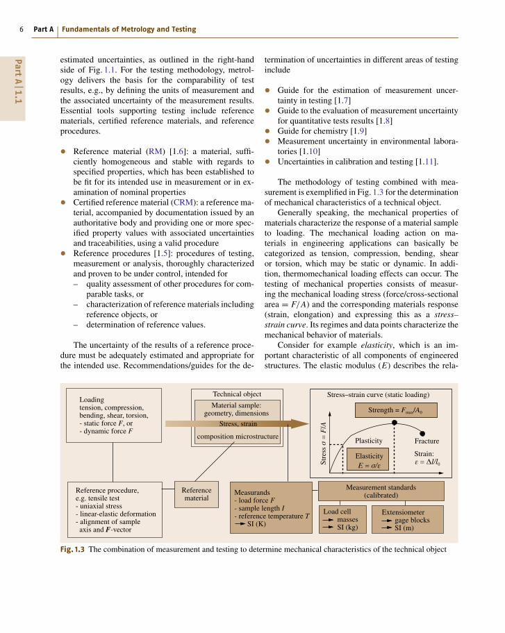
6 Part A Fundamentals of Metrology and Testing
estimated uncertainties, as outlined in the right-handside of Fig. 1.1. For the testing methodology, metrol-ogy delivers the basis for the comparability of testresults, e.g., by defining the units of measurement andthe associated uncertainty of the measurement results.Essential tools supporting testing include referencematerials, certified reference materials, and referenceprocedures.
• Reference material (RM) [1.6]: a material, suffi-ciently homogeneous and stable with regards tospecified properties, which has been established tobe fit for its intended use in measurement or in ex-amination of nominal properties• Certified reference material (CRM): a reference ma-terial, accompanied by documentation issued by anauthoritative body and providing one or more spec-ified property values with associated uncertaintiesand traceabilities, using a valid procedure• Reference procedures [1.5]: procedures of testing,measurement or analysis, thoroughly characterizedand proven to be under control, intended for– quality assessment of other procedures for com-
parable tasks, or– characterization of reference materials including
reference objects, or– determination of reference values.
The uncertainty of the results of a reference proce-dure must be adequately estimated and appropriate forthe intended use. Recommendations/guides for the de-
Loadingtension, compression,bending, shear, torsion,- static force F, or- dynamic force F
Reference procedure,e.g. tensile test- uniaxial stress- linear-elastic deformation- alignment of sample axis and F-vector
Referencematerial
Measurands- load force F- sample length I- reference temperature T SI (K)
Technical object
Material sample:geometry, dimensions
composition microstructure
Load cellmassesSI (kg)
Measurement standards(calibrated)
Extensiometer gage blocks SI (m)
Stress–strain curve (static loading)
Stress, strain
Plasticity Fracture
Strain:ε = Δl/l0E = σ/ε
Elasticity
Strength = Fmax/A0
Stre
ss σ
= F
/A
Fig. 1.3 The combination of measurement and testing to determine mechanical characteristics of the technical object
termination of uncertainties in different areas of testinginclude
• Guide for the estimation of measurement uncer-tainty in testing [1.7]• Guide to the evaluation of measurement uncertaintyfor quantitative tests results [1.8]• Guide for chemistry [1.9]• Measurement uncertainty in environmental labora-tories [1.10]• Uncertainties in calibration and testing [1.11].
The methodology of testing combined with mea-surement is exemplified in Fig. 1.3 for the determinationof mechanical characteristics of a technical object.
Generally speaking, the mechanical properties ofmaterials characterize the response of a material sampleto loading. The mechanical loading action on ma-terials in engineering applications can basically becategorized as tension, compression, bending, shearor torsion, which may be static or dynamic. In addi-tion, thermomechanical loading effects can occur. Thetesting of mechanical properties consists of measur-ing the mechanical loading stress (force/cross-sectionalarea = F/A) and the corresponding materials response(strain, elongation) and expressing this as a stress–strain curve. Its regimes and data points characterize themechanical behavior of materials.
Consider for example elasticity, which is an im-portant characteristic of all components of engineeredstructures. The elastic modulus (E) describes the rela-
PartA
1.1

Introduction to Metrology and Testing 1.1 Methodologies of Measurement and Testing 7
tion between a stress (σ ) imposed on a material andthe strain (ε) response of the material, or vice versa.The stimulus takes the form of an applied load, andthe measured effect is the resultant displacement. Thetraceability of the stress is established through the useof a calibrated load cell and by measuring the speci-men cross-sectional area with a calibrated micrometer,whereas the traceability of the strain is establishedby measuring the change in length of the originallymeasured gage length, usually with a calibrated straingage. This, however, is not sufficient to ensure re-peatable results unless a testing reference procedure,e.g., a standardized tensile test, is used on identi-cally prepared specimens, backed up by a referencematerial.
Figure 1.3 illustrates the metrological and techno-logical aspects.
• Metrologically, the measurands of the strength valueare the force (F), area (A), and the length measure-ment (l) of the technical object, all at a referencetemperature (T ).• Technologically and concerning testing, the me-chanical characteristics expressed in a stress–straincurve depend on at least the following groups ofinfluencing parameters, to be backed up by appro-priate references.– The chemical and physical nature of the ob-
ject: chemical composition, microstructure, andstructure–property relations such as crystallo-graphic shape-memory effects [1.12]; for exam-ple, strength values of metals are significantlyinfluenced by alloying elements, grain size(fine/coarse), work-hardening treatment, etc.
– The mechanical loading action and dependenceon deformation amplitude: tension, compres-sion, bending, shear, and torsion; for example,tensile strength is different from shear strengthfor a given material.
– The time dependence of the loading mode forces(static, dynamic, impact, stochastic) and devi-ations from simple linear-elastic deformation(anelastic, viscoelastic or micro-viscoplastic de-formation). Generally, the dynamic strength ofa material is different from its static strength.
The combined measurement and testing methodolo-gies, their operating parameters, and the traceabilityrequirements are illustrated in a highly simplifiedscheme by the confidence ring [1.13] shown in Fig. 1.4.
Traceable inpute.g. load
Traceable responsee.g. displacement
Proceduralaspects
e.g. alignment
Reference temperature
Traceable materialcharacterization
e.g. scale (grain size),quality (porosity)
Materialresponse
= Property
The confidencering
Fig. 1.4 Confidence ring for material property combined measure-ment and testing – note that separate traceability requirements applyto applied stimulus (load), response (displacement), and materialcharacterization (grain size, porosity)
The confidence ring illustrates that, in measurementand testing, it is generally essential to establish reliabletraceability for the applied stimulus and the resultingmeasured effect as well as for the measurements ofany other quantities that may influence the final result.The final result may also be affected by the measure-ment procedure, by temperature, and by the state ofthe sample. It is important to understand that vari-ation in measured results will often reflect materialinhomogeneity as well as uncertainties associated withthe test method or operator variability. All uncertain-ties should be taken into account in an uncertaintybudget.
1.1.3 Conformity Assessmentand Accreditation
In today’s global market and world trade there is anincreased need for conformity assessment to ensurethat products and equipment meet specifications. Thebasis for conformity assessment are measurements to-gether with methods of calibration, testing, inspection,and certification. The goal of conformity assessment
PartA
1.1

8 Part A Fundamentals of Metrology and Testing
Table 1.1 Standards of conformity assessment tools
Tools for conformity First party Second party Third party ISO standardsassessment Supplier, user Customers, Bodies independent
trade associations, from 1st andregulators 2nd parties
Supplier’s declaration × ISO/IEC 17050
Calibration, testing × × × ISO/IEC 17025
Inspection × × × ISO/IEC 17020
Certification × ISO 17021
ISO Guide 65
is to provide the user, purchaser or regulator with thenecessary confidence that a product, service, process,system or person meets relevant requirements. Theinternational standards relevant for conformity assess-ment services are provided by the ISO Committee onConformity Assessment (CASCO). The conformity as-sessment tools are listed in Table 1.1, where their useby first parties (suppliers), second parties (customers,regulators, trade organizations), and third parties (bod-ies independent from both suppliers and customers) isindicated.
Along with the growing use of these conformityassessment tools there is the request for assurance ofthe competence of the conformity assessment bodies
Market, trade
Conforming
products, services
Requirements
Technology,suppliers
Products,services
Purchasers,regulators
Demandsfor
facilitatingtrade
Society,authorities,
trade organizations
Demands for competent accreditationof conformity assessment bodies
Demands forcompetent conformityassessment
Conformity assessment bodies
Accreditation bodies
Accreditation serviceassures the competence of the conformity assessment bodies
Calibration Testing Inspection Certification
Conformity assessment service:The process for determining whether products, processes,
systems or people meet specified requirements
Fig. 1.5 Interrelations between market, trade, conformity assessment, and accreditation
(CABs). An increasingly applied and recognized toolfor this assurance is accreditation of CABs.
The world’s principal international forum for thedevelopment of laboratory accreditation practices andprocedures is the International Laboratory Accred-itation Cooperation (ILAC, http://www.ilac.org/). Itpromotes laboratory accreditation as a trade facilitationtool together with the recognition of competent cali-bration and testing facilities around the globe. ILACstarted as a conference in 1977 and became a for-mal cooperation in 1996. In 2000, 36 ILAC memberssigned the ILAC Mutual Recognition Arrangement(MRA), and by 2008 the number of members of theILAC MRA had risen to 60. Through the evaluation
PartA
1.1

Introduction to Metrology and Testing 1.2 Overview of Metrology 9
of the participating accreditation bodies, the interna-tional acceptance of test data and the elimination oftechnical barriers to trade are enhanced as recom-mended and in support of the World Trade Organization
(WTO) Technical Barriers to Trade agreement. Anoverview of the interrelations between market, trade,conformity assessment, and accreditation is shown inFig. 1.5.
1.2 Overview of Metrology
Having considered the methodologies of measurementand testing, a short general overview of metrology isgiven, based on Metrology – in short [1.5], a brochurepublished by EURAMET to establish a common metro-logical frame of reference.
1.2.1 The Meter Convention
In the middle of the 19th century the need for a world-wide decimal metric system became very apparent,particularly during the first universal industrial exhibi-tions. In 1875, a diplomatic conference on the metertook place in Paris, at which 17 governments signed thediplomatic treaty the Meter Convention. The signatories
The Metre Conventioninternational convention established in 1875 with 54 member states in 2010
CGPM Conférence Générale des Poids et MésuresCommittee with representatives from the Meter Conventionmember states. First conference held in 1889 and meets every4th year. Approves and updates the SI system with results fromfundamental metrological research.
CIPM Comité Internationale des Poids et MésuresCommittee with up to 18 representatives from CGPM.Supervises BIPM and supplies chairmen for the ConsultativeCommittees (CC).
BIPM BureauInternational desPoids et MésuresInternational research inphysicals units andstandards. Administrationof interlaboratorycomparisons of thenational metrologyinstitutes (NMI) anddesignated laboratories.
Acoustics, ultrasound, vibrationElectricity and magnetismLengthMass and related quantitiesPhotometry and radiometryAmount of substanceIonizing radiationThermometryTime and frequencyUnits.
National Metrology InstitutesNMIs developand maintain nationalmeasurement standards,represent the countryinternationally in relation toother national metrologyinstitutes and to the BIPM.A NMI or its nationalgovernment may appointdesignated institutes inthe country to hold specificnational standards.
CIPM MRA (signed 1999)Mutual recognition arran-gement between NMIs toestablish equivalence ofnational NMI measurementstandards and to providemutual recognition of theNMI calibration andmeasurement certificates.
Consultative Committees
AUVEMLMPRQMRITTFU
Fig. 1.6 The organizations and their relationships associated with the Meter Convention
decided to create and finance a permanent scientific in-stitute: the Bureau International des Poids et Mesures(BIPM). The Meter Convention, slightly modified in1921, remains the basis of all international agreementon units of measurement. Figure 1.6 provides a briefoverview of the Meter Convention Organization (detailsare described in Chap. 2).
1.2.2 Categories of Metrology
Metrology covers three main areas of activities [1.5].
1. The definition of internationally accepted units ofmeasurement
PartA
1.2

10 Part A Fundamentals of Metrology and Testing
2. The realization of units of measurement by scientificmethods
3. The establishment of traceability chains by deter-mining and documenting the value and accuracy ofa measurement and disseminating that knowledge
Metrology is separated into three categories withdifferent levels of complexity and accuracy (for details,see Chaps. 2 and 3).
Scientific MetrologyScientific metrology deals with the organization anddevelopment of measurement standards and their main-tenance. Fundamental metrology has no internationaldefinition, but it generally signifies the highest level ofaccuracy within a given field. Fundamental metrologymay therefore be described as the top-level branch ofscientific metrology.
Scientific metrology is categorized by BIPM intonine technical subject fields with different branches.The metrological calibration and measurement capa-bilities (CMCs) of the national metrology institutes(NIMs) and the designated institutes (DIs) are com-piled together with key comparisons in the BIPM keycomparison database (KCDB, http://kcdb.bipm.org/).All CMCs have undergone a process of peer evalu-ation by NMI experts under the supervision of theregional metrology organizations (RMOs). Table 1.2shows the scientific metrology fields and their branchestogether with the number of registered calibrationand measurement capabilities (CMCs) of the NMIs in2010.
Table 1.2 Metrology areas and their branches, together with the numbers of metrological calibration and measurementcapabilities (CMCs) of the national metrology institutes and designated institutes in the BIPM KCDB as of 2010
Metrology area Branch CMCs
Acoustics, ultrasound, vibrations Sound in air; sound in water; vibration 955
Electricity and magnetism DC voltage, current, and resistance; impedance up to the megahertz range; 6586
AC voltage, current, and power; high voltage and current;
other DC and low-frequency measurements; electric and magnetic fields;
radiofrequency measurements
Length Laser; dimensional metrology 1164
Mass and related quantities Mass; density; pressure; force; torque, viscosity, hardness and gravity; fluid flow 2609
Photometry and radiometry Photometry; properties of detectors and sources; spectral properties; color; 1044
fiber optics
Amount of substance List of 16 amount-of-substance categories 4558
Ionizing radiation Dosimetry; radioactivity; neutron measurements 3983
Thermometry Temperature; humidity; thermophysical quantities 1393
Time and frequency Time scale difference; frequency; time interval 586
Industrial MetrologyIndustrial metrology has to ensure the adequate func-tioning of measurement instruments used in industrialproduction and in testing processes. Systematic mea-surement with known degrees of uncertainty is one ofthe foundations of industrial quality control. Generallyspeaking, in most modern industries the costs bound upin taking measurements constitute 10–15% of produc-tion costs.
However, good measurements can significantly in-crease the value, effectiveness, and quality of a product.Thus, metrological activities, including calibration, test-ing, and measurements, are valuable inputs to ensurethe quality of most industrial processes and qualityof life related activities and processes. This includesthe need to demonstrate traceability to internationalstandards, which is becoming just as important as themeasurement itself. Recognition of metrological com-petence at each level of the traceability chain can beestablished through mutual recognition agreements orarrangements, as well as through accreditation and peerreview.
Legal MetrologyLegal metrology originated from the need to ensurefair trade, specifically in the area of weights and mea-sures. The main objective of legal metrology is to assurecitizens of correct measurement results when used in of-ficial and commercial transactions. Legally controlledinstruments should guarantee correct measurement re-sults throughout the whole period of use under workingconditions, within given permissible errors.
PartA
1.2

Introduction to Metrology and Testing 1.2 Overview of Metrology 11
For example, in Europe, the marketing and usage ofthe following measuring instruments are regulated bythe European Union (EU) measuring instruments direc-tive (MID 2004/22/EC)
1. Water meters2. Gas meters3. Electrical energy meters and measurement trans-
formers4. Heat meters5. Measuring systems for liquids other than water6. Weighing instruments7. Taximeters8. Material measures9. Dimensional measuring systems10. Exhaust gas analyzers
Member states of the European Union have the op-tion to decide which of the instrument types they wishto regulate.
The International Organization of Legal Metrology(OIML) is an intergovernmental treaty organization es-tablished in 1955 on the basis of a convention, whichwas modified in 1968. In the year 2010, OIML wascomposed of 57 member countries and an additional58 (corresponding) member countries that joined theOIML (http://www.oiml.org/) as observers. The pur-pose of OIML is to promote global harmonization oflegal metrology procedures. The OIML has developeda worldwide technical structure that provides its mem-bers with metrological guidelines for the elaborationof national and regional requirements concerning the
Table 1.3 The SI base units
Quantity Base unit Symbol Definition
Length Meter m The meter is the length of the path traveled by light in a vacuum during a time intervalof 1/299 792 458 of a second
Mass Kilogram kg The kilogram is equal to the mass of the international prototype of the kilogram
Time Second s The second is the duration of 9 192 631 770 periods of the radiation corresponding tothe transition between the two hyperfine levels of the ground state of the cesium-133atom
Electric current Ampere A The ampere is that constant current which, if maintained in two straight parallel con-ductors of infinite length, of negligible circular cross-section, and placed one meterapart in vacuum, would produce between these conductors a force equal to 2 × 10⁻⁷
newtons per meter of length
Temperature Kelvin K The kelvin is the fraction 1/273.16 of the thermodynamic temperature of the triplepoint of water
Amount of substance Mole mol The mole is the amount of substance of a system that contains as many elementaryentities as there are atoms in 0.012 kg of carbon-12. When the mole is used, the ele-mentary entities must be specified and may be atoms, molecules, ions, electrons, otherparticles, or specified groups of such particles
Luminous intensity Candela cd The candela is the luminous intensity in a given direction of a source that emitsmonochromatic radiation of frequency 540 × 1012 Hz and has a radiant intensity inthat direction of 1/683 W per steradian
manufacture and use of measuring instruments for legalmetrology applications.
1.2.3 Metrological Units
The idea behind the metric system – a system of unitsbased on the meter and the kilogram – arose dur-ing the French Revolution when two platinum artefactreference standards for the meter and the kilogramwere constructed and deposited in the French NationalArchives in Paris in 1799 – later to be known as the Me-ter of the Archives and the Kilogram of the Archives.The French Academy of Science was commissioned bythe National Assembly to design a new system of unitsfor use throughout the world, and in 1946 the MKSAsystem (meter, kilogram, second, ampere) was acceptedby the Meter Convention countries. The MKSA was ex-tended in 1954 to include the kelvin and candela. Thesystem then assumed the name the International Systemof Units (Le Système International d’Unités, SI). TheSI system was established in 1960 by the 11th GeneralConference on Weights and Measures (CGPM): The In-ternational System of Units (SI) is the coherent systemof units adopted and recommended by the CGPM.
At the 14th CGPM in 1971 the SI was again ex-tended by the addition of the mole as base unit foramount of substance. The SI system is now comprisedof seven base units, which together with derived unitsmake up a coherent system of units [1.5], as shown inTable 1.3.
PartA
1.2

12 Part A Fundamentals of Metrology and Testing
Table 1.4 Examples of SI derived units expressed in SI base units
Derived quantity Si derived unit special name Symbol In SI units In SI base units
Force Newton N m kg s−2
Pressure, stress Pascal Pa N/m2 m−1 kg s−2
Energy, work, quantity of heat Joule J N m m2 kg s−2
Power Watt W J/s m2 kg s−3
Electric charge Coulomb C s A
Electromotive force Volt V m2 kg s−3 A−1
Electric capacitance Farad F C/V m−2 kg−1 s4 A2
Electric resistance Ohm Ω V/A m2 kg s−3 A−2
Electric conductance Siemens S A/V m−2 kg−1 s3 A2
SI derived units are derived from the SI base unitsin accordance with the physical connection betweenthe quantities. Some derived units, with examples frommechanical engineering and electrical engineering, arecompiled in Table 1.4.
1.2.4 Measurement Standards
In the introductory explanation of the methodologyof measurement, two essential aspects were pointedout.
1. Measurement begins with the definition of the mea-surand.
Measurement methodology Metrologysubfield
Measurement standards(examples)
Dimensionalmetrologylength
Mass
Force, pressure
Electricity (DC)
Photometry
Temperature
Timemeasurement
SI unitsOBJECT
Characteristics
Measurand
Calibration
Measurement principleMeasurement methodMeasurement systemMeasurement uncertainty
Measurement resultQuantity value1 uncertainty (unit)
Measurementstandard
Gauge blocks, opticalinterferometry, measuringmicroscopes, coordinatemeasuring instruments
Standard balances,mass comparators
Load cells, dead-weighttesters, pressure balances,capacitance manometers
Josephson effect, quantumHall effect, Zener diode,comparator bridges
Si photodiodes, quantumefficiency detectors
Gas thermometers, IST 90fixed points, thermocouplespyrometers
Cesium atomic clock, timeinterval equipment
Measurement procedure
Fig. 1.7 Measurement standards as an integral part of the measurement methodology
2. When the measurand is defined, it must be relatedto a measurement standard.
A measurement standard, or etalon, is the realizationof the definition of a given quantity, with stated quantityvalue and associated measurement uncertainty, used asa reference. The realization may be provided by a mater-ial measure, measuring instrument, reference materialor measuring system.
Typical measurement standards for subfields ofmetrology are shown in Fig. 1.7 in connection withthe scheme of the measurement methodology (left-handside of Fig. 1.1). Consider, for example, dimensionalmetrology. The meter is defined as the length of the path
PartA
1.2

Introduction to Metrology and Testing 1.3 Fundamentals of Materials Characterization 13
traveled by light in vacuum during a time interval of1/299 792 458 of a second. The meter is realized at theprimary level (SI units) in terms of the wavelength froman iodine-stabilized helium-neon laser. On sublevels,material measures such as gage blocks are used, andtraceability is ensured by using optical interferometry todetermine the length of the gage blocks with referenceto the above-mentioned laser light wavelength.
A national measurement standard is recognized bya national authority to serve in a state or economy asthe basis for assigning quantity values to other measure-ment standards for the kind of quantity concerned. Aninternational measurement standard is recognized bysignatories to an international agreement and intendedto serve worldwide, e.g., the international prototype ofthe kilogram.
1.3 Fundamentals of Materials Characterization
Materials characterization methods have a wide scopeand impact for science, technology, economy, and so-ciety, as materials comprise all natural and syntheticsubstances and constitute the physical matter of engi-neered and manufactured products.
For materials there is a comprehensive spectrum ofmaterials measurands. This is due to the broad varietyof metallic, inorganic, organic, and composite materials,their different chemical and physical nature, and themanifold attributes which are related to materials withrespect to composition, microstructure, scale, synthe-sis, physical and electrical properties, and applications.Some of these attributes can be expressed in a metro-logical sense as numbers, such as density; some areBoolean, such as the ability to be recycled or not; some,such as resistance to corrosion, may be expressed asa ranking (poor, adequate, good, for instance); and somecan only be captured in text and images [1.14]. As back-ground for materials characterization methods, whichare treated in parts B, C, D of the handbook, namely
• Chemical and microstructural analysis• Materials properties measurement• Materials performance testing
the essential features of materials are outlined in thenext sections [1.15].
1.3.1 Nature of Materials
Materials can be natural (biological) in origin or syn-thetically processed and manufactured. According totheir chemical nature, they are broadly grouped tradi-tionally into inorganic and organic materials.
The physical structure of materials can be crys-talline or amorphous, as well as mixtures of bothstructures. Composites are combinations of materialsassembled together to obtain properties superior tothose of their single constituents. Composites (C) are
classified according to the nature of their matrix: metal(MM), ceramic (CM) or polymer (PM) matrix com-posites, often designated as MMCs, CMCs, and PMCs,respectively. Figure 1.8 illustrates, with characteristicexamples, the spectrum of materials between the cat-egories natural, synthetic, inorganic, and organic.
From the view of materials science, the fundamentalfeatures of a solid material are as listed below.
• Material’s atomic nature: the atomic elements of thePeriodic Table which constitute the chemical com-position of a material• Material’s atomic bonding: the type of cohe-sive electronic interactions between the atoms (ormolecules) in a material, empirically categorizedinto the following basic classes.– Ionic bonds form between chemical elements
with very different electron negativity (tendency
Natural
Synthetic
Inor
gani
c
Org
anicComposites
MMC, CMC, PMC
MineralsWood,paper
Metals,ceramics
Polymers
Fig. 1.8 Classification of materials
PartA
1.3

14 Part A Fundamentals of Metrology and Testing
Grain diameter(µm scale)
Grain boundaryprecipitations
Areal grainboundary
precipitations
Screwdislocation
0.25 nm
Unit cellof α-iron(bcc)
Metallic materials are usually polycrystalline andmay contain at the mm scale up to hundreds ofgrains with various lattice defects
Example: cross sectionof a metallic material,polished and etched tovisualize grains
Substituted atomInterstitual point defect
Edgedislocation
Incoherentprecipitations
Lattice-orientedprecipitations
Embedded hard phase
Vacancy
Slip bands(lattice steps due toplastic deformation)
mm scale
Fig. 1.9 Schematic overview on the microstructural features of metallic materials and alloys
to gain electrons), resulting in electron transferand the formation of anions and cations. Bond-ing occurs through electrostatic forces betweenthe ions.
– Covalent bonds form between elements thathave similar electron negativities; the electronsare localized and shared equally between theatoms, leading to spatially directed angularbonds.
– Metallic bonds occur between elements withlow electron negativities, so that the electronsare only loosely attracted to the ionic nuclei.A metal is thought of as a set of positivelycharged ions embedded in a sea of electrons.
– van der Waals bonds are due to the differentinternal electronic polarities between adjacentatoms or molecules, leading to weak (sec-ondary) electrostatic dipole bonding forces.• Material’s spatial atomic structure: the amorphous
or crystalline arrangement of atoms (or molecules)resulting from long-range or short-range bonding
forces. In crystalline structures, it is characterizedby unit cells which are the fundamental buildingblocks or modules, repeated many times in spacewithin a crystal.• Grains: crystallites made up of identical unit cellsrepeated in space, separated by grain boundaries.• Phases: homogeneous aggregations of matter withrespect to chemical composition and uniform crystalstructure; grains composed of the same unit cells arethe same phase.• Lattice defects: deviations from ideal crystal struc-ture.– Point defects or missing atoms: vacancies, inter-
stitial or substituted atoms– Line defects or rows of missing atoms: disloca-
tions– Area defects: grain boundaries, phase bound-
aries, and twins– Volume defects: cavities, precipitates.• Microstructure: The microscopic collection ofgrains, phases, and lattice defects.
PartA
1.3

Introduction to Metrology and Testing 1.3 Fundamentals of Materials Characterization 15
In addition to bulk materials characteristics, surface andinterface phenomena also have to be considered.
In Fig. 1.9 an overview of the microstructural fea-tures of metallic materials is depicted schematically.Methods and techniques for the characterization ofnanoscopic architecture and microstructure are pre-sented in Chap. 5.
1.3.2 Types of Materials
It has been estimated that there are between 40 000and 80 000 materials which are used or can be used intoday’s technology [1.14]. Figure 1.10 lists the mainconventional families of materials together with ex-amples of classes, members, and attributes. For theexamples of attributes, necessary characterization meth-ods are listed.
Metallic Materials and AlloysIn metals, the grains are the buildings blocks and areheld together by the electron gas. The free valenceelectrons of the electron gas account for the high electri-cal and thermal conductivity, as well as for the opticalgloss of metals. Metallic bonding, seen as the interac-tion between the total atomic nuclei and the electrongas, is not significantly influenced by displacement ofatoms, which is the reason for the good ductility andformability of metals. Metals and metallic alloys arethe most important group of the so-called structuralmaterials whose special features for engineering appli-cations are their mechanical properties, e.g., strengthand toughness.
Subject Family Class Member Attributes
Materials
CompositionChemical analysis
DensityMeasurement
Grain sizeMeasurement
Wear resistance3-body-systems testing
ReliabilityProbabilistic simulation
• Natural
• Ceramics
• Polymers
• Metals
• Semiconductors
• Composites
• Biomaterials
Steels
Cast iron
Al-alloys
Cu-alloys
Ni-alloys
Ti-alloys
Zn-alloys
CuBeCo
CuCd
CuCr
Bronze
CuPb
CuTe
CuZr
Fig. 1.10 Hierarchy of materials, and examples of attributes and necessary characterization methods
SemiconductorsSemiconductors have an intermediate position betweenmetals and inorganic nonmetallic materials. Their mostimportant representatives are the elements silicon andgermanium, possessing covalent bonding and diamondstructure; they are also similar in structure to III–V com-pounds such as gallium arsenide (GaAs). Being electricnonconductors at absolute zero temperature, semicon-ductors can be made conductive through thermal energyinput or atomic doping, which leads to the creationof free electrons contributing to electrical conductivity.Semiconductors are important functional materials forelectronic components and applications.
Inorganic Nonmetallic Materials or CeramicsAtoms of these materials are held together by covalentand ionic bonding. As covalent and ionic bonding en-ergies are much higher than those of metallic bonds,inorganic nonmetallic materials, such as ceramics, havehigh hardness and high melting temperatures. Thesematerials are basically brittle and not ductile: In contrastto the metallic bond model, displacement of atomic di-mensions theoretically breaks localized covalent bondsor transforms anion–cation attractions into anion–anionor cation–cation repulsions. Because of the lack of freevalence electrons, inorganic nonmetallic materials arepoor conductors of electricity and heat; this qualifiesthem as good insulators in engineering applications.
Organic Materials or Polymers and BlendsOrganic materials, whose technologically most impor-tant representatives are the polymers, consist of macro-
PartA
1.3

16 Part A Fundamentals of Metrology and Testing
molecules containing carbon (C) covalently bondedwith itself and with elements of low atomic num-ber (e.g., H, N, O, S). Intimate mechanical mixturesof several polymers are called blends. In thermoplas-tic materials, the molecular chains have long linearstructures and are held together by (weak) intermolec-ular (van der Waals) bonds, leading to low meltingtemperatures. In thermosetting materials, the chainsare connected in a network structure and thereforedo not melt. Amorphous polymer structures (e.g.,polystyrene) are transparent, whereas crystalline poly-mers are translucent to opaque. The low density ofpolymers gives them a good strength-to-weight ratioand makes them competitive with metals in structuralengineering applications.
CompositesGenerally speaking, composites are hybrid creationsmade of two or more materials that maintain theiridentities when combined. The materials are chosenso that the properties of one constituent enhance thedeficient properties of the other. Usually, a given prop-erty of a composite lies between the values for eachconstituent, but not always. Sometimes, the propertyof a composite is clearly superior to those of eitherof the constituents. The potential for such a syn-ergy is one reason for the interest in composites forhigh-performance applications. However, because man-ufacturing of composites involves many steps andis labor intensive, composites may be too expen-sive to compete with metals and polymers, even iftheir properties are superior. In high-technology ap-plications of advanced composites, it should alsobe borne in mind that they are usually difficult torecycle.
Nanometer Kilometer
10−9 10−6 10−3
Nanoscale Microscale Macroscale
Scale (m)
• Atomic, molecular nanoarchitecture
• Electronic, quantum structures
• Macro engineering
• Bulk components
• Assembled structures
• Engineered systems
• Microstructures of materials
MeterMillimeter
1 103
Micrometer
Fig. 1.11 Scale of material dimensions to be recognized in materials metrology and testing
Natural MaterialsNatural materials used in engineering applications areclassified into natural materials of mineral origin, e.g.,marble, granite, sandstone, mica, sapphire, ruby, or di-amond, and those of organic origin, e.g., timber, Indiarubber, or natural fibres such as cotton and wool. Theproperties of natural materials of mineral origin, for ex-ample, high hardness and good chemical durability, aredetermined by strong covalent and ionic bonds betweentheir atomic or molecular constituents and stable crystalstructures. Natural materials of organic origin often pos-sess complex structures with directionally dependentproperties. Advantageous aspects of natural materialsare ease of recycling and sustainability.
BiomaterialsBiomaterials can be broadly defined as the class ofmaterials suitable for biomedical applications. Theymay be synthetically derived from nonbiological oreven inorganic materials, or they may originate in liv-ing tissues. Products that incorporate biomaterials areextremely varied and include artificial organs; biochem-ical sensors; disposable materials and commodities;drug-delivery systems; dental, plastic surgery, ear, andophthalmological devices; orthopedic replacements;wound management aids; and packaging materials forbiomedical and hygienic uses. When applying bio-materials, understanding of the interactions betweensynthetic substrates and biological tissues is of crucialimportance to meet clinical requirements.
1.3.3 Scale of Materials
The geometric length scale of materials covers morethan 12 orders of magnitude. The scale ranges from
PartA
1.3

Introduction to Metrology and Testing 1.3 Fundamentals of Materials Characterization 17
1064.18 °C:Melting point of goldFix point of the internationaltemperature scale ITS-90
Gold particle radius (nm)
Example of the scaledependence ofmaterials properties:melting point of gold
Source: K.J. Klabunde (2001)
Example of the scale dependence of materials properties
Mechanical strength and stiffness of carbon nanotubes
• Compression strength: 2 times than that of Kevlar• Tensile strength: 10 times than that of steel• Stiffness: 2000 times than that of diamond
Source: G. Bachmann, VDI-TZ (2004)Scale: 10 nm diameter
Bulk gold
Mel
ting
poin
t (°C
)
1100
1000
900
800
700
600
500
400
300
200
100
00 1 2 3 4 5 6 7 8 9 10 11
Fig. 1.12 Examples of the influence of scale effects on thermal and mechanical materials properties
the nanoscopic materials architecture to kilometer-longstructures of bridges for public transport, pipelines, andoil drilling platforms for supplying energy to society.Figure 1.11 illustrates the dimensional scales relevantfor today’s materials science and technology.
Material specimens of different geometric dimen-sions have different bulk-to-surface ratios and may alsohave different bulk and surface microstructures. Thiscan significantly influence the properties of materials,as exemplified in Fig. 1.12 for thermal and mechanicalproperties. Thus, scale effects have to be meticulouslyconsidered in materials metrology and testing.
1.3.4 Properties of Materials
Materials and their characteristics result from theprocessing of matter. Their properties are the re-sponse to extrinsic loading in their application. Forevery application, materials have to be engineeredby processing, manufacturing, machining, forming ornanotechnology assembly to create structural, func-
tional or smart materials for the various engineeringtasks (Fig. 1.13).
The properties of materials, which are of fundamen-tal importance for their engineering applications, can becategorized into three basic groups.
1. Structural materials have specific mechanical orthermal properties for mechanical or thermal tasksin engineering structures.
2. Functional materials have specific electromagneticor optical properties for electrical, magnetic or opti-cal tasks in engineering functions.
3. Smart materials are engineered materials withintrinsic or embedded sensor and actuator func-tions, which are able to accommodate materialsin response to external loading, with the aim ofoptimizing material behavior according to given re-quirements for materials performance.
Numerical values for the various materials prop-erties can vary over several orders of magnitude forthe different material types. An overview of the broad
PartA
1.3

18 Part A Fundamentals of Metrology and Testing
Matter Materials
Processing
Manufacturing
Machining
Forming
Nanotechnology
assembly
• Solids
• Liquids
• Molecules
• Atoms
• Structural materials
Mechanical, thermal tasks
• Functional materials
Electrical, magnetic, optical tasks
• Smart materials
Sensors and actuator tasks
Fig. 1.13 Materials and their characteristics result from the processing of matter
Mechanical properties Electrical properties Thermal propertiesElastic modulus E Specific resistance Thermal conductivity λ
Metals Metals Inorganics Organics Metals Inorganics Organics
1016
1014
1012
1010
108
106
104
102
10–2
10–4
10–6
10–8
1
103
102
10
1
10–1
10–2
OsmiumTungsten
ChromiumSteelCopperGold
Lead
SilverTin
CeramicsLimit:Diamond
SiCAl2O3
GlassMullite
Porcelain
Concrete
Timber
Rubber
PVCPMMAEpoxyPAPCPEPTFE
SteelCopperSilver
Glass
EpoxyPVCPCPA
PTFE
PorcelainMullite
Cermets
Graphite
Con-ductivepolymers
E
(GPa)ρ
(Ω m)
10–1
1
10
102
5×10²
CeramicsSiC
GlassPorcelainSilica
SilverCopperGoldAluminumTungsten
Chromium
Bronze
Lead
Steel
λ(W/(m K))
Concrete
EpoxyPEPVCPTFETimber
Inorganics Organics
Aluminum
ρ
Al2O3
Fig. 1.14 Overview of mechanical, electrical, and thermal materials properties for the basic types of materials (metal,inorganic, or organic)
PartA
1.3

Introduction to Metrology and Testing 1.3 Fundamentals of Materials Characterization 19
numerical spectra of some mechanical, electrical, andthermal properties of metals, inorganics, and organics isshown in Fig. 1.14 [1.16].
It must be emphasized that the numerical ranking ofmaterials in Fig. 1.14 is based on rough, average val-ues only. Precise data of materials properties require thespecification of various influencing factors describedabove and symbolically expressed as
Materials properties data
= f (composition–microstructure–scale,
external loading, . . .) .
1.3.5 Performance of Materials
For the application of materials as constituents ofengineered products, performance characteristics suchas quality, reliability, and safety are of special im-portance. This adds performance control and materialfailure analysis to the tasks of application-oriented ma-terials measurement, testing, and assessment. Becauseall materials interact with their environment, materials–environment interactions and detrimental influences on
Materials–environment interactions
• Ores• Natural substances• Coal • Oil• Chemicals
Raw materials
• Metals • Polymers• Ceramics • Composites• Structural materials• Functional materials
Engineering materials
End of useDeposition
Processing
Productssystems
• Scrap• Waste• Refuse
Materialsintegrity control• Aging• Biodegradation• Corrosion• Wear• Fracture
Functional loads
TheEarth
Matter
Recycling
Performance
Fig. 1.15 The materials cycle of all products and technical systems
the integrity of materials must also be considered. Anoverview of the manifold aspects to be recognized in thecharacterization of materials performance is provided inFig. 1.15.
The so-called materials cycle depicted schemati-cally in Fig. 1.15 applies to all manmade technicalproducts in all branches of technology and econ-omy. The materials cycle illustrates that materials(accompanied by the necessary flow of energy and in-formation) move in cycles through the technoeconomicsystem: from raw materials to engineering materialsand technical products, and finally, after the termina-tion of their task and performance, to deposition orrecycling.
The operating conditions and influencing factorsfor the performance of a material in a given applica-tion stem from its structural tasks and functional loads,as shown in the right part of Fig. 1.15. In each appli-cation, materials have to fulfil technical functions asconstituents of engineered products or parts of tech-nical systems. They have to bear mechanical stressesand are in contact with other solid bodies, aggressivegases, liquids or biological species. In their functionaltasks, materials always interact with their environment,
PartA
1.3

20 Part A Fundamentals of Metrology and Testing
Mechanical Thermal Radiological Chemical Biological Tribological
Fracture
Aging
Corrosion
Biodeterioration
Wear
Stresscorrosion
Heat Ionizingradiation Gases
Liquids
Micro-orga-nisms
High-T-corrosion
Influences on materials integrity, leading eventually to materials deterioration
Shear
Bending
Torsion
Fretting fatigue
Sliding
Rolling
Tension
Compression
Example: Corroded pipe
Example: Fractured steel rail, broken under the complex combinationof various loading actions: mechanical (local impulse bending), thermal(temperature variations), chemical (moisture), and tribological (cyclicrolling, Hertzian wheel-contact pressure, interfacial microslip)
Spin Impact
Fig. 1.16 Fundamentals of materials performance characterization: influencing phenomena
so these aspects also have to be recognized to character-ize materials performance.
For the proper performance of engineered mater-ials, materials deterioration processes and potentialfailures, such as materials aging, biodegradation, corro-sion, wear, and fracture, must be controlled. Figure 1.16shows an overview of influences on materials integrityand possible failure modes.
Figure 1.16 illustrates in a generalized, simplifiedmanner that the influences on the integrity of materials,which are essential for their performance, can be cate-gorized in mechanical, thermal, radiological, chemical,biological, and tribological terms. The basic materialsdeterioration mechanisms, as listed in Fig. 1.15, are ag-ing, biodegradation, corrosion, wear, and fracture.
The deterioration and failure modes illustrated inFig. 1.16 are of different relevance for the two ele-mentary classes of materials, namely organic materialsand inorganic materials (Fig. 1.8). Whereas aging andbiodegradation are main deterioration mechanisms fororganic materials such as polymers, the various types ofcorrosion are prevailing failure modes of metallic mater-ials. Wear and fracture are relevant as materials deterio-ration and failure mechanisms for all types of materials.
1.3.6 Metrology of Materials
The topics of measurement and testing applied to ma-terials (in short metrology of materials) concern theaccurate and fit-for-purpose determination of the behav-ior of a material throughout its lifecycle.
Recognizing the need for a sound technical basisfor drafting codes of practice and specifications for ad-vanced materials, the governments of countries of theEconomic Summit (G7) and the European Commis-sion signed a Memorandum of Understanding in 1982to establish the Versailles Project on Advanced Mater-ials and Standards (VAMAS, http://www.vamas.org/).This project supports international trade by enablingscientific collaboration as a precursor to the draftingof standards. Following a suggestion of VAMAS, theComité International des Poids et Mesures (CIPM,Fig. 1.6) established an ad hoc Working Group on theMetrology Applicable to the Measurement of MaterialProperties. The findings and conclusions of the Work-ing Group on Materials Metrology were published ina special issue of Metrologia [1.17]. One important find-ing is the confidence ring for traceability in materialsmetrology (Fig. 1.4).
PartA
1.3

Introduction to Metrology and Testing 1.3 Fundamentals of Materials Characterization 21
Materialsapplication
Processing and synthesis of matter
Engineering design, production technologies
Functionalloads
Deteriorationactions
Reference materials Reference methods
Reference methods,nondestructive evaluation
Material
Metrology and testing
Composition Microstructure Properties Performance
Environment
Fig. 1.17 Characteristics of materials to be recognized in metrology and testing
Materials in engineering design have to meet oneor more structural, functional (e.g., electrical, optical,magnetic) or decorative purposes. This encompassesmaterials such as metals, ceramics, and polymers, re-sulting from the processing and synthesis of matter,based on chemistry, solid-state physics, and surfacephysics. Whenever a material is being created, devel-oped or produced, the properties or phenomena thatthe material exhibits are of central concern. Experienceshows that the properties and performance associatedwith a material are intimately related to its composi-tion and structure at all scale levels, and influencedalso by the engineering component design and produc-tion technologies. The final material, as a constituentof an engineered component, must perform a giventask and must do so in an economical and societallyacceptable manner. All these aspects are compiled inFig. 1.17 [1.15].
The basic groups of materials characteristics essen-tially relevant for materials metrology and testing, asshown in the central part of Fig. 1.17, can be categorizedas follows.
• Intrinsic characteristics are the material’s com-position and material’s microstructure, describedin Sect. 1.3.1. The intrinsic (inherent) materialscharacteristics result from the processing and syn-
thesis of matter. Metrology and testing to determinethese characteristics have to be backed up by suit-able reference materials and reference methods, ifavailable.• Extrinsic characteristics are the material’s prop-erties and material’s performance, outlined inSects. 1.3.4 and 1.3.5. They are procedural charac-teristics and describe the response of materials andengineered components to functional loads and en-vironmental deterioration of the material’s integrity.Metrology and testing to determine these character-istics have to be backed up by suitable referencemethods and nondestructive evaluation (NDE).
It follows that, in engineering applications of mater-ials, methods and techniques are needed to characterizeintrinsic and extrinsic material attributes, and to con-sider also structure–property relations. The methodsand techniques to characterize composition and mi-crostructure are treated in part B of the handbook. Themethods and techniques to characterize properties andperformance are treated in parts C and D. The finalpart E of the handbook presents important modeling andsimulation methods that underline measurement pro-cedures that rely on mathematical models to interpretcomplex experiments or to estimate properties that can-not be measured directly.
PartA
1.3

22 Part A Fundamentals of Metrology and Testing
References
1.1 BIPM: International Vocabulary of Metrology,3rd edn. (BIPM, Paris 2008), available fromhttp://www.bipm.org/en/publications/guides/
1.2 C. Ehrlich, S. Rasberry: Metrological timelines intraceability, J. Res. Natl. Inst. Stand. Technol. 103,93–106 (1998)
1.3 EUROLAB: Measurement uncertainty revisited: Al-ternative approaches to uncertainty evaluation,EUROLAB Tech. Rep. No. 1/2007 (EUROLAB, Paris 2007),http://www.eurolab.org/
1.4 ISO: Guide to the Expression of Uncertainty in Mea-surement (GUM-1989) (International Organizationfor Standardization, Geneva 1995)
1.5 P. Howarth, F. Redgrave: Metrology – In Short, 3rdedn. (Euramet, Braunschweig 2008)
1.6 ISO Guide 30: Terms and Definitions of ReferenceMaterials (International Organization for Standard-ization, Geneva 1992)
1.7 T. Adam: Guide for the Estimation of MeasurementUncertainty in Testing (American Association for Lab-oratory Accreditation (A2LA), Frederick 2002)
1.8 EUROLAB: Guide to the evaluation of measurementuncertainty for quantitative tests results, EURO-LAB Tech. Rep. No. 1/2006 (EUROLAB, Paris 2006),http://www.eurolab.org/
1.9 EURACHEM/CITAC Guide: Quantifying Uncertainty inAnalytical Measurement, 2nd edn. (EURACHEM/CITAC,Lisbon 2000)
1.10 B. Magnusson, T. Naykki, H. Hovind, M. Krysell:Handbook for Calculation of Measurement. Un-certainty, NORDTEST Rep. TR 537 (Nordtest, Espoo2003)
1.11 R. Cook: Assessment of Uncertainties of Measurementfor Calibration and Testing Laboratories (NationalAssociation of Testing Authorities Australia, Rhodes2002)
1.12 J. Ma, I. Karaman: Expanding the repertoire ofshape memory alloys, Science 327, 1468–1469(2010)
1.13 S. Bennett, G. Sims: Evolving needs for metrology inmaterial property measurements – The conclusionsof the CIPM Working Group on Materials Metrology,Metrologia 47, 1–17 (2010)
1.14 M.F. Ashby, Y.J.M. Brechet, D. Cebon, L. Salvo: Se-lection strategies for materials and processes, Mater.Des. 25, 51–67 (2004)
1.15 H. Czichos: Metrology and testing in mater-ials science and engineering, Measure 4, 46–77(2009)
1.16 H. Czichos, B. Skrotzki, F.-G. Simon: Materials. In:HÜTTE – Das Ingenieurwissen, 33rd edn., ed. byH. Czichos, M. Hennecke (Springer, Berlin, Heidel-berg 2008)
1.17 S. Bennett, J. Valdés (Eds.): Materials metrology,Foreword, Metrologia 47(2) (2010)
PartA
1

23
Metrology Pri2. Metrology Principles and Organization
This chapter describes the basic elements ofmetrology, the system that allows measurementsmade in different laboratories to be confidentlycompared. As the aim of this chapter is to give anoverview of the whole field, the development ofmetrology from its roots to the birth of the Me-tre Convention and metrology in the 21st century isgiven.
2.1 The Roots and Evolution of Metrology .... 23
2.2 BIPM: The Birth of the Metre Convention 25
2.3 BIPM: The First 75 Years......................... 26
2.4 Quantum Standards:A Metrological Revolution...................... 28
2.5 Regional Metrology Organizations .......... 29
2.6 Metrological Traceability ....................... 29
2.7 Mutual Recognition of NMI Standards:The CIPM MRA ....................................... 302.7.1 The Essential Points of the MRA ...... 302.7.2 The Key Comparison Database
(KCDB) ......................................... 312.7.3 Take Up of the CIPM MRA ............... 31
2.8 Metrology in the 21st Century................. 322.8.1 Industrial Challenges .................... 322.8.2 Chemistry, Pharmacy, and Medicine 332.8.3 Environment, Public Services,
and Infrastructures....................... 34
2.9 The SI System and New Science .............. 34
References .................................................. 37
2.1 The Roots and Evolution of Metrology
From the earliest times it has been important to com-pare things through measurements. This had much todo with fair exchange, barter, or trade between commu-nities, and simple weights such as the stone or measuressuch as the cubit were common. At this level, parts ofthe body such as hands and arms were adequate formost needs. Initially, wooden length bars were easy tocompare and weights could be weighed against eachother. Various forms of balance were commonplace inearly history and in religion. Egyptian tomb paintingsshow the Egyptian god Anubis weighing the soul ofthe dead against an ostrich feather – the sign of purity(Fig. 2.1). Noah’s Ark was, so the Book of Genesis re-ports, 300 cubits long by 50 cubits wide and 30 cubitshigh. No one really knows why it was important torecord such details, but the Bible, as just one example,is littered with metrological references, and the symbol-ism of metrology was part of early culture and art.
A steady progression from basic artifacts to natu-rally occurring reference standards has been part of theentire history of metrology. Metrologists are familiarwith the use of the carob seed in early Mediterranean
civilizations as a natural reference for length and forweight and hence volume. The Greeks were earlytraders who paid attention to metrology, and they wereknown to keep copies of the weights and measures ofthe countries with which they traded.
Fig. 2.1 Anubis
PartA
2

24 Part A Fundamentals of Metrology and Testing
Fig. 2.2 Winchester yard
Fig. 2.3 Imperial length standards, Trafalgar Square, London
The Magna Carta of England set out a framework fora citizen’s rights and established one measure through-out the land. Kings and queens took interest in nationalweights and measures; Fig. 2.2 shows the Winchesteryard, the bronze rod that was the British standard from1497 to the end of the 16th century. The queen’s markwe see here is that of Elizabeth the First (1558–1603).In those days, the acre was widely used as a measure-ment, derived from the area that a team of oxen couldplow in a day. Plowing an acre meant that you had towalk 66 furlongs, a linear dimension measured in rods.
The problem with many length measurements wasthat the standard was made of the commonly availablemetals brass or bronze, which have a fairly large co-efficient of expansion. Iron or steel measures were notdeveloped for a couple of centuries. Brass and bronzetherefore dominated the length reference business un-til the early 19th century, by which time metallurgy haddeveloped enough – though it was still something ofa black art – for new, lower-expansion metals to be usedand reference temperatures quoted. The UK imperial
references were introduced in 1854 and reproduced inTrafalgar Square in the center of London (Fig. 2.3), andthe British Empire’s domination of international com-merce saw the British measurement system adopted inmany of its colonies.
In the mid 18th century, Britain and France com-pared their national measurement standards and realizedthat they differed by a few percent for the same unit.Although the British system was reasonably consistentthroughout the country, the French found that differ-ences of up to 50% were common in length measurementwithin France. The ensuing technical debate was the startof what we now accept as the metric system. France ledthe way, and even in the middle of the French Revolutionthe Academy of Science was asked to deduce an invari-able standard for all the measures and all the weights.The important word was invariable. There were two op-tions available for the standard of length: the second’spendulum and the length of the Earth’s meridian. The ob-vious weakness of the pendulum approach was that itsperiod depended on the local acceleration due to grav-ity. The academy therefore chose to measure a portionof the Earth’s circumference and relate it to the officialFrench meter. Delambre and Méchain, who were en-trusted with a survey of the meridian between Dunkirkand Barcelona, created the famous Mètre des Archives,a platinum end standard.
The international nature of measurement was driven,just like that of the Greek traders of nearly 2000 yearsbefore, by the need for interoperability in trade and ad-vances in engineering measurement. The displays ofbrilliant engineering at the Great Exhibitions in Londonand Paris in the 19th century largely rested on the abilityto measure well. The British Victorian engineer JosephWhitworth coined the famous phrase you can only makeas well as you can measure and pioneered accurate screwthreads. He immediately saw the potential of end stan-dard gages rather than line standards where the referencelength was defined by a scratch on the surface of a bar.The difficulty, he realized, with line standards was thatoptical microscopes were not then good enough to com-pare measurements of line standards well enough for thebest precision engineering. Whitworth was determinedto make the world’s best measuring machine. He con-structed the quite remarkable millionth machine basedon the principle that touch was better than sight for preci-sion measurement. It appears that the machine had a feelof about 1/10 of a thousandth of an inch. Another inter-esting metrological trend at the 1851 Great Exhibitionwas military: the word calibrate comes from the need tocontrol the caliber of guns.
PartA2.1

Metrology Principles and Organization 2.2 BIPM: The Birth of the Metre Convention 25
At the turn of the 19th century, many of the industri-alized countries had set up national metrology institutes,generally based on the model established in Germanywith the Physikalisch Technische Reichsanstalt, whichwas founded in 1887. The economic benefits of sucha national institute were immediately recognized, and asa result, scientific and industrial organizations in a num-ber of industrialized countries began pressing their gov-ernments to make similar investments. In the UK, theBritish Association for the Advancement of Science re-ported that, without a national laboratory to act as a focusfor metrology, the country’s industrial competitivenesswouldbeweakened.Thecausewas takenupmorewidely,and the UK set up the National Physical Laboratory(NPL) in 1900. The USA created the National Bureau ofStandards in 1901 as a result of similar industrial pres-sure. The major national metrology institutes (NMIs),however, had a dual role. In general, they were the mainfocus for national research programs on applied physicsand engineering. Their scientific role in the developmentof units – what became the International System of Units,the SI – began to challenge the role of the universities inthe measurement of fundamental constants. This was es-pecially true after the development of quantum physics inthe 1920s and 1930s. Most early NMIs therefore beganwith two major elements to their mission
• a requirement to satisfy industrial needs for accuratemeasurements, through standardization and verifica-tion of instruments; and• determination of physical constants so as to improveand develop the SI system.
The new industries which emerged after the First WorldWar made huge demands on metrology and, togetherwith mass production and the beginnings of multina-tional production sites, raised new challenges whichbrought NMIs into direct contact with companies, socausing a close link to develop between them. At thattime, and even up to the mid 1960s, nearly all cali-brations and measurements that were necessary for in-dustrial use were made in the NMIs, and in the gagerooms of the major companies, as were most measure-ments in engineering metrology. The industries of the1920s, however, developed a need for electrical and opti-cal measurements, so NMIs expanded their coverage andtheir technical abilities.
The story since then is one of steady technical ex-pansion until after the Second World War. In the 1950s,though, there was renewed interest in a broader ap-plied focus for many NMIs so as to develop civilianapplications for much of the declassified military tech-nology. The squeeze on public budgets in the 1970sand 1980s saw a return to core metrology, and manyother institutions, public and private, took on the re-sponsibility for developing many of the technologies,which had been initially fostered at NMIs. The NMIsadjusted to their new roles. Many restructured andfound new, often improved, ways of serving indus-trial needs. This recreation of the NMI role was alsoshared by most governments, which increasingly sawthem as tools of industrial policy with a mission tostimulate industrial competitiveness and, at the end ofthe 20th century, to reduce technical barriers to worldtrade.
2.2 BIPM: The Birth of the Metre Convention
A brief overview of the Metre Convention has alreadybeen given in Sect. 1.2.1. In the following, the historicaldevelopment will be described.
During the 1851 Great Exhibition and the 1860meeting of the British Association for the Advance-ment of Science (BAAS), a number of scientists andengineers met to develop the case for a single systemof units based on the metric system. This built on theearly initiative of Gauss to use the 1799 meter andkilogram in the Archives de la République, Paris andthe second, as defined in astronomy, to create a co-herent set of units for the physical sciences. In 1874,the three-dimensional CGS system, based on the cen-timeter, gram, and second, was launched by the BAAS.
However, the size of the electrical units in the CGS sys-tem were not particularly convenient and, in the 1880s,the BAAS and the International Electrotechnical Com-mission (IEC) approved a set of practical electrical unitsbased on the ohm, the ampere, and the volt. Parallel tothis attention to the units, a number of governments setup what was then called the Committee for Weights andMoney, which in turn led to the 1870 meeting of theCommission Internationale du Mètre. Twenty-six coun-tries accepted the invitation of the French Governmentto attend; however, only 16 were able to come as theFranco–Prussian war intervened, so the full commit-tee did not meet until 1872. The result was the MetreConvention and the creation of the Bureau International
PartA
2.2

26 Part A Fundamentals of Metrology and Testing
Fig. 2.4 Bureau International des Poids et Mesures, Sévres
des Poids et Mesures (BIPM, International Bureau ofWeights and Measures), in the old Pavillon de Breteuilat Sèvres (Fig. 2.4), as a permanent scientific agencysupported by the signatories to the convention. As thisrequired the support of governments at the highest level,the Metre Convention was not finally signed until 20May 1875.
The BIPM’s role was to establish new metric stan-dards, conserve the international prototypes (then themeter and the kilogram) and to carry out the compar-isons necessary to assure the uniformity of measuresthroughout the world. As an intergovernmental, diplo-matic treaty organization, the BIPM was placed underthe authority of the General Conference on Weightsand Measures (CGPM). A committee of 18 scientificexperts, the International Committee for Weights andMeasures (CIPM), now supervises the running of theBIPM. The aim of the CGPM and the CIPM was, andstill is, to assure the international unification and de-velopment of the metric system. The CGPM now meetsevery 4 years to review progress, receive reports fromthe CIPM on the running of the BIPM, and establish theoperating budget of the BIPM, whereas the CIPM meetsannually to supervise the BIPM’s work.
When it was set up, the staff of the BIPM con-sisted of a director, two assistants, and the necessarynumber of employees. In essence, then, a handful of
people began to prepare and disseminate copies ofthe international prototypes of the meter and the kilo-gram to member states. About 30 copies of the meterand 40 copies of the prototype kilogram were dis-tributed to member states by ballot. Once this wasdone, some thought that the job of the BIPM wouldsimply be that of periodically checking (in the jar-gon, verifying) the national copies of these standards.This was a short-lived vision, as the early investiga-tions immediately showed the importance of reliablymeasuring a range of quantities that influenced theperformance of the international prototypes and theircopies. As a result, a number of studies and projectswere launched which dealt with the measurement oftemperature, density, pressure, and a number of relatedquantities. The BIPM immediately became a researchbody, although this was not recognized formally until1921.
Returning to the development of the SI, one of theearly decisions of the CIPM was to modify the CGSsystem to base measurements on the meter, kilogram,and second – the MKS system. In 1901, Giorgi showedthat it was possible to combine the MKS system withthe practical electrical units to form a coherent four-dimensional system by adding an electrical unit andrewriting some of the equations of electromagnetism inthe so-called rationalized form. In 1946, the CIPM ap-proved a system based on the meter, kilogram, second,and ampere – the MKSA system. Recognizing the am-pere as a base unit of the metric system in 1948, andadding, in 1954, units for thermodynamic temperature(the kelvin and luminous intensity (the candela), the11th CGPM in 1960 coined the name Système inter-nationale d’Unités, the SI. At the 14th CGPM in 1971,the present-day SI system was completed by adding themole as the base unit for the amount of substance, bring-ing the total number of base units to seven. Using thesebase units, a hierarchy of derived units and quantities ofthe SI have been developed for most, if not all, measure-ments needed in today’s society. A substantial treatmentof the SI is to be found in the 8th edition of the SIbrochure published by the BIPM [2.1].
2.3 BIPM: The First 75 Years
After its intervention in the initial development of theSI, the BIPM continued to develop fundamental metro-logical techniques in mass and length measurement butsoon had to react to the metrological implications of
major developments in atomic physics and interferom-etry. In the early 1920s, Albert Michelson came towork at the BIPM and built an eponymous interfer-ometer to measure the meter in terms of light from
PartA
2.3

Metrology Principles and Organization 2.3 BIPM: The First 75 Years 27
the cadmium red line – an instrument which, althoughmodified, did sterling service until the 1980s. In tem-perature measurement, the old hydrogen thermometerscale was replaced with a thermodynamic-based scaleand a number of fixed points. After great debate, elec-trical standards were added to the work of the BIPM inthe 1920s with the first international comparisons of re-sistance and voltage. In 1929, an electrical laboratorywas added, and photometry arrived in 1939.
In these early days, it was clear that the BIPMneeded to find a way of consulting and collaboratingwith the experts in the world’s NMIs. The solutionadopted is one which still exists and flourishes today.The best way of working was in face-to-face meetings,so the concept of a consultative committee to the CIPMwas born. Members of the committee were drawn fromexperts active in the world’s NMIs and met to dealwith matters concerning the definitions of units and thetechniques of comparison and calibration. The consul-tative committees are usually chaired by a member ofthe CIPM. Much information was shared, although forobvious logistical reasons, the meetings were not toofrequent. Over the years, the need for new consulta-tive committees grew in reaction to the expansion ofmetrology, and now 10 consultative committees exist,with over 25 working groups.
The CIPM is rightly cautious about establishinga new committee, but proposals for new ones are con-sidered from time to time, usually after an initial surveythrough a working group. In the last 10 years, joint com-mittees have been created to tackle issues such as the
Table 2.1 List of consultative committees with dates of formation
Names of consultative committees and the date of their formation(Names of consultative committees have changed as they have gained new responsibilities;the current name is cited)
Consultative Committee for Electricity and Magnetism, CCEM (1997, but created in 1927)
Consultative Committee for Photometry and Radiometry, CCPR (1971 but created in 1933)
Consultative Committee for Thermometry, CCT (1937)
Consultative Committee for Length, CCL (1997 but created in 1952)
Consultative Committee for Time and Frequency, CCTF (1997, but created 1956)
Consultative Committee for Ionizing Radiation, CCRI (1997, but created in 1958)
Consultative Committee for Units, CCU (1964, but replacing a similar commission created in 1954)
Consultative Committee for Mass and Related Quantities, CCM (1980)
Consultative Committee for Amount of Substance and Metrology in Chemistry, CCQM (1993)
Consultative Committee for Acoustics, Ultrasound, and Vibration, CCAUV (1999)
international approach to the estimation of measure-ment uncertainties or to the establishment of a commonvocabulary for metrology. Most of these joint com-mittees bring the BIPM together with international orintergovernmental bodies such as the International Or-ganization for Standardization (ISO), the InternationalLaboratory Accreditation Cooperation (ILAC), and theIEC. As the work of the Metre Convention movesinto areas other than its traditional activities in physicsand engineering, joint committees are an excellent wayof bringing the BIPM together with other bodies thatbring specialist expertise – an example being the jointcommittee for laboratory medicine, established recentlywith the International Federation of Clinical Chemistsand the ILAC.
The introduction of ionizing radiation standards tothe work of the BIPM came when Marie Curie de-posited her first radium standard at the BIPM in 1913.As a result of pressure, largely from the USSR delega-tion to the CGPM, the CIPM took the decision to dealwith metrology in ionizing radiation.
In the mid 1960s, and at the time of the expansioninto ionizing radiation, programs on laser length mea-surement were also started. These contributed greatly tothe redefinition of the meter in 1983. The BIPM alsoacted as the world reference center for laser wavelengthor frequency comparisons in much the same was as itdid for physical artifact-based standards. In the mean-time, however, the meter bar had already been replaced,in 1960, by an interferometric-based definition usingoptical radiation from a krypton lamp.
PartA
2.3

28 Part A Fundamentals of Metrology and Testing
2.4 Quantum Standards: A Metrological Revolution
Technology did not stand still, and in reaction tothe developments and metrological applications of su-perconductivity, important projects on the Josephson,quantum Hall, and capacitance standards were launchedin the late 1980s and 1990s. The BIPM played a keyrole in establishing worldwide confidence in the perfor-mance of these new devices through an intense programof comparisons which revealed many of the system-atic sources of error and found solutions to them. Theemergence of these and other quantum-based standards,however, was an important and highly significant de-velopment. In retrospect, these were one of the driversfor change in the way in which world metrology orga-nizes itself and had implications nationally as well asinternationally.
The major technical change was, in essence, a be-lief that standards based on quantum phenomena werethe same the world over. Their introduction sometimesmade it unnecessary for a single, or a small number of,reference standards to be held at the BIPM or in a few ofthe well-established and experienced NMIs. Quantum-based standards were, in reality, available to all and,with care, could be operated outside the NMIs at veryhigh levels of accuracy.
There were two consequences. Firstly, that thenewer NMIs that wanted to invest in quantum-basedstandards needed to work with experienced metrolo-gists in existing NMIs in order to develop their skills asrapidly as possible. Many of the older NMIs, therefore,became adept at training and providing the necessaryexperience for newer metrologists. The second con-sequence was an increased pressure for comparisonsof standards, as the ever-conservative metrology com-munity sought to develop confidence in new NMIs aswell as in the quantum-based standards. These includedfrequency-stabilized lasers, superconducting voltageand resistance standards, cryogenic radiometers (formeasurements related to the candela), atomic clocks(for the second), and a range of secondary standards.
Apart from its responsibility to maintain the interna-tional prototype kilogram (Fig. 2.5), which remains thelast artifact-based unit of the SI, the BIPM was thereforeno longer always the sole repository of an internationalprimary reference standard. However there were, andstill are, a number of unique reference facilities at theBIPM for secondary standards and quantities of the SI.Staff numbers had also leveled off at about 70.
If it was going to maintain its original mission ofa scientifically based organization with responsibility
for coordinating world metrology, the BIPM recognizedthat it needed to discharge particular aspects of its treatyobligation in a different way. It also saw the increasedvalue of developing the links needed to establish col-laboration at the international and intergovernmentallevel. In addition, the staff had the responsibility to pro-vide the secretariat to the 10 consultative committees ofthe CIPM as well as an increasing number of workinggroups. The last 10 years of the 20th century, there-fore, saw the start of a significant change in the BIPM’sway of working. During this period, it was also facedwith the need to develop a world metrology infrastruc-ture in new areas such as the environment, chemistry,medicine, and food. The shift away from physics andengineering was possible, fortunately, as a result ofthe changing way in which the SI units could be real-ized, particularly through the quantum-based standards.Other pressures for an increase in the BIPM’s coor-dination role resulted from the increasingly intensiveprogram of comparisons brought about by the launchof the CIPM’s mutual recognition arrangement in the1990s.
The most recent consequence of these trends wasthat the CIPM decided that the photometry and radiom-etry section would close due to the need to operatewithin internationally agreed budgets, ending nearly
Fig. 2.5 International prototype kilogram (courtesy ofBIPM)
PartA
2.4
Metrology Principles and Organization 2.6 Metrological Traceability 29
70 years of scientific activity at the BIPM. Additionalsavings would also be made by restricting the work ofthe laser and length group to a less ambitious program.
A small, 130-year-old institution was therefore inthe process of reinventing itself to take on and developa changed but nevertheless unique niche role. This wasstill based on technical capabilities and laboratory workbut was one which had to meet the changing, and ex-panding, requirements of its member states in a different
way. Much more also needed to be done as the ben-efits of precise, traceable measurement became seen asimportant in a number of the new disciplines for metrol-ogy. This change of emphasis was endorsed at the 2003General Conference on Weights and Measures as a new4 year work program (2005–2008) was agreed, as wellas the first real-terms budget increase since the increaseagreed in the mid 1960s which then financed the expan-sion into ionizing radiation.
2.5 Regional Metrology Organizations
The growth of the number of NMIs and the emergenceof world economic groupings such as the Asia–PacificEconomic Cooperation and the European Union meanthat regional metrological groupings have becomea useful way of addressing specific regional needs andcan act as a mutual help or support network. The firstsuch group was probably in Europe, where an organi-zation now named EURAMET emerged from a loosecollaboration of NMIs based on the Western EuropeanMetrology Club. There are now five regional metrologyorganizations (RMOs): the Asian–Pacific MetrologyProgram (APMP) with perhaps the largest geographi-cal coverage from India in the west to New Zealand inthe east and extending into Asia, the Euro–Asian Co-operation in Metrology amongst the Central EuropeanCountries (COOMET), the European Association ofNational Metrology Institutes (EURAMET), the South-ern African Development Community Cooperation inMeasurement Traceability (SADCMET), and SistemaInteramericano de Metrología (SIM, Inter-American
Metrology System) which covers Southern, Central, andNorth America). The RMOs play a vital role in en-couraging coherence within their region and betweenregions; without their help, the Metre Convention wouldbe far more difficult to administer and its outreach tononmembers – who may, however, be members of anRMO – would be more difficult.
Traditionally, NMIs have served their own nationalcustomers. It is only within the last 10 years that re-gional metrology organizations have started to becomemore than informal associations of national laborato-ries and have begun to develop strategies for mutualdependence and resource sharing, driven by concernsabout budgets and the high cost of capital facilities. Thesharing of resources is still, however, a relatively smallproportion of all collaborations between NMIs, most ofwhich are still at the research level. It is, of course,no coincidence that RMOs are based on economic ortrading blocs and that these groupings are increasinglyconcerned with free trade within and between them.
2.6 Metrological Traceability
Traceability of measurement has been a core concern ofthe Metre Convention from its inception, as has beenemphasized already in Sect. 2.1. Initially, a measure-ment is always made in relation to a more accuratereference, and these references are themselves cali-brated or measured against an even more accuratereference standard. The chain follows the same patternuntil one reaches the national standards. (For technicaldetails see Chap. 3.)
The NMIs’ job was to make sure that the na-tional standards were traceable to the SI and wereaccurate enough to meet national needs. As NMIsthemselves stopped doing all but the highest accuracymeasurements and as accredited laboratories, usually
in the commercial sector, took on the more routinetasks, the concept of a national hierarchy of trace-able measurements became commonplace, frequentlycalled a national measurement system. In general, thetechnical capabilities of the intermediate laboratoriesare assured by their accreditation to the internationaldocumentary standards ISO/IEC 17025 by a nationalaccreditation body, usually a member of the Interna-tional Laboratory Accreditation Cooperation (ILAC)(Sect. 1.1.3). At the top of the traceability system,measurements were relatively few in number and hadthe lowest uncertainty. Progressing down the traceabil-ity chain introduced a greater level of uncertainty ofmeasurement, and generally speaking, a larger number
PartA
2.6
30 Part A Fundamentals of Metrology and Testing
of measurements are involved. Traceability itself alsoneeded to be defined. The international vocabulary ofmetrology (VIM) defines traceability as [2.2]:
The property of a measurement result relating theresult to a stated metrological reference through anunbroken chain of calibrations or comparisons eachcontributing to the stated uncertainty.
The important emphasis is on uncertainty of mea-surement (for a detailed treatment of measurementuncertainty, the reader is referred to the Guide to the ex-pression of uncertainty in measurement (GUM) [2.3])and the need for the continuous unbroken chain of mea-surement. Comparisons of standards or references area common way of demonstrating confidence in the mea-surement processes and in the reference standards heldeither in the NMIs or in accredited laboratories. Thenational accreditation body usually takes care of thesecomparisons at working levels, sometimes called in-terlaboratory comparisons (ILCs) or proficiency testing(Sect. 3.6).
At the NMI level, the framework of the BIPMand the CIPM’s consultative committees (CCs) tookcare of the highest level comparisons. However, the in-creased relevance of traceable measurement to trade,
and the need for demonstrable equivalence of the na-tional standards held at NMIs, and to which nationalmeasurements were traceable, took a major turn in themid 1990s. This event was stimulated by the need, fromthe accreditation community as much as from regulatorsand trade bodies, to know just how well the NMI stan-dards agreed with each other. Unlike much of the workof the consultative committees, this involved NMIs ofall states of maturity working at all levels of accuracy.The task of comparing each and every standard was toogreat and too complex for the CC network, so a novelapproach needed to be adopted. In addition, it becameincreasingly clear that the important concept was oneof measurements traceable to the SI through the stan-dards realized and maintained at NMIs, rather than tothe NMI-based standards themselves. Not to developand work with this concept would run the risk of creat-ing technical barriers to trade (TBTs) if measurementsin a certain country were legally required to be trace-able to the NMI standards or if measurements madeelsewhere were not recognized. The World Trade Or-ganization was turning its attention towards the needfor technical measurements to be accepted worldwideand was setting challenging targets for the reduction ofTBTs. The metrology community needed to react.
2.7 Mutual Recognition of NMI Standards: The CIPM MRA
The result was the creation, by the CIPM, of a mutualrecognition arrangement (MRA) for the recognition andacceptance of NMI calibration and test certificates. TheCIPM MRA is one of the key events of the last fewyears, and one which may be as significant as the MetreConvention itself. The CIPM MRA has a direct impacton the reduction of technical barriers to trade and tothe globalization of world business. The CIPM MRAwas launched at a meeting of NMIs from member statesof the Metre Convention held in Paris on 14 October1999, at which the directors of the national metrologyinstitutes of 38 member states of the convention and rep-resentatives of two international organizations becamethe first signatories.
2.7.1 The Essential Points of the MRA
The objectives of the CIPM MRA are
• to establish the degree of equivalence of nationalmeasurement standards maintained by NMIs,
• to provide for the mutual recognition of calibrationand measurement certificates issued by NMIs, and• thereby to provide governments and other partieswith a secure technical foundation for wider agree-ments related to international trade, commerce, andregulatory affairs.
The procedure through which an NMI, or any other rec-ognized signatory, joins the MRA is based on the needto demonstrate their technical competence, and to con-vince other signatories of their performance claims. Inessence, these performance claims are the uncertaintiesassociated with the routine calibration services whichare offered to customers and which are traceable to theSI. Initial claims, called calibration and measurementcapabilities (CMCs), are first made by the laboratoryconcerned. They are then first reviewed by technicalexperts from the local regional metrology organizationand, subsequently, by other RMOs. The technical ev-idence for the CMC claims is generally based on theinstitute’s performance in a number of comparisons
PartA
2.7

Metrology Principles and Organization 2.7 Mutual Recognition of NMI Standards: The CIPM MRA 31
carried out and managed by the relevant CIPM consulta-tive committees (CCs) or by the RMO. This apparentlycomplex arrangement is needed because it would betechnically, financially or organizationally impossiblefor each participant to compare its own SI standardswith all others. The CIPM places particular importanceon two types of comparisons
• international comparisons of measurements, knownas CIPM key comparisons and organized by theCCs, which generally involve only those laborato-ries which perform at the highest level. The subjectof a key comparison is chosen carefully by the CCto be representative of the ability of the laboratoryto make a range of related measurements;• key or supplementary international comparisons ofmeasurements, usually organized by the RMOs andwhich include some of the laboratories which tookpart in the CIPM comparisons as well as other lab-oratories from the RMO. RMO key comparisonsare in the same technical area as the CIPM com-parison, whereas supplementary comparisons areusually carried out to meet a special regional need.
Using this arrangement, we can establish links betweenall participants to provide the technical basis for thecomparability of the SI standards at each NMI. Reportsof all the comparisons are published in the key compar-ison database maintained by the BIPM on its website(www.bipm.org).
These comparisons differ from those traditionallycarried out by the CCs, which were largely for scien-tific reasons and which established the dependence ofthe SI realizations on the effects which contributed tothe uncertainty of the realization. In CIPM and RMOkey or supplementary comparisons, however, each par-ticipant carries out the measurements without knowingthe results of others until the comparison has beencompleted. They provide, therefore, an independent as-sessment of performance. The CIPM, however, tookthe view that comparisons are made at a specific mo-ment in time and so required participating NMIs toinstall a quality system which could help demonstrateconfidence in the continued competence of participantsin between comparisons. All participants have chosento use the ISO/IEC 17025 standard and have the op-tion of a third-party accreditation by an ILAC memberor a self-declaration together with appropriate peer re-views.
The outcome of this process is that it gives NMIsthe confidence to recognize the results of key and sup-plementary comparisons as stated in the database and
therefore to accept the calibration and measurement ca-pabilities of other participating NMIs.
When drawing up its MRA, the CIPM was acutelyaware that its very existence, and the mutual acceptanceof test and calibration certificates between its members,might be seen as a technical barrier to trade in itself. Theconcept of associate members of the CGPM was there-fore developed. An associate has, in general, the rightto take part in the CIPM MRA but not to benefit fromthe full range of BIPM services and activities, which arerestricted to convention members. Associate status is in-creasingly popular with developing countries, as it helpsthem gain recognition worldwide but does not committhem to the additional expense of convention member-ship, which may be less appropriate for them at theirstage of development.
2.7.2 The Key Comparison Database (KCDB)
The key comparison database, referred to in the MRAand introduced in Sect. 1.2.2 (Table 1.2), is available onthe BIPM website (www.bipm.org). The content of thedatabase is evolving rapidly. Appendix A lists signato-ries, and appendix B contains details of the set of keycomparisons together with the results from those thathave been completed. The database will also containa list of those old comparisons selected by the consul-tative committees that are to be used on a provisionalbasis. Appendix C contains the calibration and measure-ment capabilities of the NMIs that have already beendeclared and reviewed within their own regional metrol-ogy organization (RMO) as well as those other RMOsthat support the MRA.
2.7.3 Take Up of the CIPM MRA
The KCDB data is, at the moment, largely of interest tometrologists. However, a number of NMIs are keen tosee it taken up more widely, and there are several ex-amples of references to the CIPM MRA in regulation.This campaign is at an early stage; an EU–USA tradeagreement cites the CIPM MRA as providing an appro-priate technical basis for acceptance of measurementsand tests, and the USA’s National Institute of Standardsand Technology (NIST) has opened up a discussionwith the Federal Aviation Authority (FAA) and otherregulators as to the way in which they can use KCDBdata to help the FAA accept the results of tests andcertificates which have been issued outside the USA.
There is a range of additional benefits and conse-quences of the CIPM MRA. Firstly, anyone can use
PartA
2.7

32 Part A Fundamentals of Metrology and Testing
the KCDB to look for themselves at the validated tech-nical capability of any NMI. As a result, they can,with full confidence, choose to use its calibration ser-vices rather than those of their national laboratory andhave the results of these services accepted worldwide.They can also use the MRA database to search forNMIs that can satisfy their needs if they are not avail-able nationally. This easy access and the widespreadand cheap availability of information may well drivea globalization of the calibration service market andwill enable users to choose the supplier that best meetstheir needs. As the MRA is implemented, it will bea real test of market economics. Secondly, there isthe issue of rapid turnarounds. Companies that haveto send their standards away for calibration do not
have them available for in-house use. This can leadto costly duplication if continuity of an internal ser-vice is essential, or to a tendency to increase thecalibration interval if calibrations are expensive. NMIstherefore have to concentrate increasingly on reduc-ing turnaround times, or providing better customerinformation through calibration management systems.Some calibrations will always require reasonable peri-ods of time away from the workplace because of theneed for stability or because NMIs can only (throughtheir own resource limitations) provide the service atcertain times. This market sensitivity is now fast be-coming built into service delivery and is, in some cases,more important to a customer than the actual price ofa calibration.
2.8 Metrology in the 21st Century
In concluding this review of the work of the Metre Con-vention, it seems appropriate to take a glance at whatthe future may have in store for world metrology and, inparticular, at the new industries and technologies whichrequire new measurements.
2.8.1 Industrial Challenges
The success of the Metre Convention and, in particu-lar, the recognized technical and economic benefits ofthe CIPM MRA – one estimate by the consulting com-pany KPMP puts its potential impact on the reduction ofTBTs at some € 4 billion (see the BIPM website) – haveattracted the interest and attention of new communitiesof users.
New TechnologiesA challenge which tackles the needs of new indus-tries and exploits new technologies is to enhance ourability to measure the large, the small, the fast, andthe slow. Microelectronics, telecommunications, andthe study and characterization of surfaces and thinfilms will benefit. Many of these trends are regularlyanalyzed by NMIs as they formulate their technicalprograms, and a summary can be found in the re-cent report to the 22nd CGPM by its secretary Dr.Robert Kaarls, entitled Evolving Needs for Metrologyin Trade, Industry, and Society and the Role of theBIPM. The report can be found on the BIPM website(http://www.bipm.org/).
Materials CharacterizationOf particular relevance to the general topic of thishandbook, there has been an interest in a worldwideframework for traceable measurement of material char-acteristics. The potential need is for validated, acceptedreference data to characterize materials with respect totheir properties (see Part C) and their performance (seePart D). To a rather limited extent, some properties arealready covered in a metrological sense (hardness, somethermophysical or optical properties, for example), butthe vast bulk of materials characteristics, which arenot intrinsic properties but system-dependent attributes(Sect. 1.3.6), remain outside the work of the conven-tion. Therefore, relatively few NMIs have been activein materials metrology, but a group is meeting to decidewhether to make proposals for a new sphere of MetreConvention activity. A report recommending action waspresented to the CIPM in 2004 and will be followedup in a number of actions launched by the committee(Sect. 1.3.6).
Product AppearanceAnother challenge is the focus by manufacturers on thedesign or appearance of a product, which differentiatesit in the eyes of the consumer from those of their com-petitors. These rather subjective attributes of a productare starting to demand an objective basis for compar-ison. Appearance measurement of quantities such asgloss, or the need to measure the best conditions inwhich to display products under different lighting or pre-
PartA
2.8

Metrology Principles and Organization 2.8 Metrology in the 21st Century 33
sentation media (such as a TV tube, flat-panel display,or a printed photograph), or the response for differenttypes of sounds combine hard physical or chemical mea-surements with the subjective and varying responses of,say, the human eye or ear. However, these are preciselythe quantities that a consumer uses to judge textiles,combinations of colored products, or the relative soundreproduction of music systems. They are therefore alsothe selling points of the marketer and innovator. Howcan the consumer choose and differentiate? How canthey compare different claims? Semisubjective measure-ments such as these are moving away from the carefullycontrolled conditions of the laboratory into the highstreet and are presenting exciting new challenges.
NMIs are already becoming familiar with the needsof their users for color or acoustical measurement ser-vices, which require a degree of modeling of the userresponse and differing reactions depending on environ-mental conditions such as ambient lighting or noisebackground. The fascination of this area is that it com-bines objective metrology with physiological measure-ments and the inherent variability of the human eye orear, or the ways in which our brains process optical orauditory stimuli.
Real-Time In-Process MeasurementsThe industries of today and tomorrow are starting toerode one of the century-old metrology practices withinwhich the user must bring their own instruments andstandards to the NMI for calibration. Some of this re-lates to the optimization of industrial processes, wherefar more accurate, real-time, in-process measurementsare made. The economics of huge production processesdemand just-in-time manufacture, active data manage-ment, and sophisticated process modeling. By reliablyidentifying where subelements of a process are be-having poorly, plant engineers can take rapid remedialaction and so identify trouble spots quickly. However,actual real-time systems measurements are difficult, andit is only recently that some NMIs have begun to ad-dress the concept of an industrial measurement system.New business areas such as this will require NMIs towork differently, if for no other reason than becausetheir customers work differently and they need to meetthe customers’ requirements. Remote telemetry, data fu-sion, and new sensor techniques are becoming linkedwith process modeling, numerical algorithms, and ap-proximations so that accurate measurement can be put,precisely, at the point of measurement. These users arealready adopting the systems approach, and some NMIsare starting to respond to this challenge.
Quantum-Based StandardsThere is a trend towards quantum-based standardsin industry, as already highlighted in this chapter.This is a result of the work of innovative instrumentcompanies which now produce, for example, stabi-lized lasers, Josephson-junction voltage standards, andatomic clocks for the mass market. The availabilityof such highly accurate standards in industry is itselftestimony to companies’ relentless quest for improvedproduct performance and quality. However, withoutcare and experience, it is all too easy to get the wronganswer. Users are advised to undertake comparisonsand to cooperate closely with their NMIs to make surethat these instruments are operated with all the properchecks and with attention to best practice so that theymay, reliably, bring increased accuracy closer to the enduser [2.4]. Industry presses NMIs – rightly so – forbetter performance, and in some areas of real practi-cal need, NMI measurement capabilities are still ratherclose to what industry requires. It is, perhaps, in thesehighly competitive and market-driven areas that the keycomparisons and statements of equivalence that are partof the CIPM MRA will prove their worth. Companiesspecify the performance of their products carefully inthese highly competitive markets, and any significantdifferences in the way in which NMIs realize the SIunits and quantities will have a direct bearing on com-petitiveness, market share, and profitability.
2.8.2 Chemistry, Pharmacy, and Medicine
Chemistry, biosciences, and pharmaceuticals are, formany of us, the new metrology. We are used to thepractices of physical and engineering metrology, and sothe new technologies are challenging our understand-ing of familiar concepts such as traceability, uncertainty,and primary standards. Much depends here on the in-teraction between a particular chemical or species andthe solution or matrix in which it is to be found,as well as the processes or methods used to makethe measurement. The concept of reference materials(RMs) (Chap. 3) is well developed in the chemical field,and the Consultative Committee for Quantity of Mat-ter Metrology in Chemistry (CCQM) has embarked ona series of RM and other comparisons to assess the stateof the art in chemical and biological measurements.
Through the CIPM MRA, the international metrol-ogy community has started to address the needs andconcerns of regulators and legislators. This has alreadybrought the Metre Convention into the areas of labora-tory medicine and food [genetically modified organisms
PartA
2.8

34 Part A Fundamentals of Metrology and Testing
(GMOs), pesticides, and trace elements]. The BIPM isonly beginning to tackle and respond to the world ofmedicine and pharmacy and has created a partnershipwith the International Federation of Clinical Chemistry(IFCC) and ILAC to address these needs in a JointCommittee for Traceability in Laboratory Medicine(JCTLM). This is directed initially at a database of ref-erence materials which meet certain common criteriaof performance. Recognition of the data in the JCTLMdatabase will, in particular, help demonstrate compli-ance of the products of the in vitro diagnostic industrywith the requirements of a recent directive [2.5] of theEuropean Union. The BIPM has signed a memorandumof understanding with the World Health Organization tohelp pursue these matters at an international level.
2.8.3 Environment, Public Services,and Infrastructures
In the area of the environment, our current knowledgeof the complex interactions of weather, sea currents, andthe various layers of our atmosphere is still not capa-ble of a full explanation of environmental issues. Themetrologist is, however, beginning to make a recognizedcontribution by insisting that slow or small changes,particularly in large quantities, should be measuredtraceably and against the unchanging reference stan-
dards offered through the units and quantities of the SIsystem. Similar inroads are being made into the spacecommunity where, for example, international and na-tional space agencies are starting to appreciate that solarradiance measurements can be unreliable unless relatedto absolute measurements. We await the satellite launchof a cryogenic radiometer, which would do much to val-idate and monitor long-term trends in solar physics. Therelevance of these activities is far from esoteric. Gov-ernments spend huge sums of money in their efforts totackle environmental issues, and it is only by puttingmeasurements on a sound basis that we can begin tomake sure that these investments are justified and aremaking a real difference in the long term.
Traceable measurements are beginning to be neededas governments introduce competition into the supplyof public services and infrastructures. Where utilities,such as electricity or gas, are offered by several differ-ent companies, the precise moment at which a consumerchanges supplier can have large financial consequences.Traceable timing services are now used regularly inthese industries as well as in stock exchanges and thegrowing world of e-commerce. Global trading is under-pinned by globally accepted metrology, often withoutusers appreciating the sophistication, reliability, and ac-ceptability of the systems in which they place suchimplicit trust.
2.9 The SI System and New Science
Science never stands still, and there are a number oftrends already evident which may have a direct bear-ing on the definitions of the SI itself. Much of thisis linked with progress in measuring the fundamen-tal constants, their coherence with each other and theSI, and the continued belief that they are time andspace invariant. Figure 2.6 shows the current rela-tionships of the basic SI units defined in Sect. 1.2.3(Table 1.3).
This figure presents some of the links between thebase units of the SI (shown in circles) and the funda-mental physical and atomic constants (shown in boxes).It is intended to show that the base units of the SI arelinked to measurable quantities through the unchangingand universal constants of physics.
The base units of the International System of Unitsdefined in Table 1.3 are
A = ampere
K = Kelvin
s = second
m = meter
kg = kilogram
cd = candela
mol = mole
The surrounding boxes, lines, and uncertainties rep-resent measurable quantities.
The numbers marked next to the base units are esti-mates of the standard uncertainties of their best practicalrealizations.
The fundamental and atomic constants shown are
RK = von Klitzing constant
KJ = Josephson constant
RK−90 and KJ−90: the conventional values of these constants,introduced on 1 January 1990
NA = Avogadro constant
F = Faraday constant
PartA
2.9

Metrology Principles and Organization 2.9 The SI System and New Science 35
G = Newtonian constant of gravitation
m12C = mass of 12C
m e = electron mass
R∞ = Rydberg constant
h = Planck constant
c= speed of light
μ0 = magnetic constant
α= fine-structure constant
R = molar gas constant
kB = Boltzmann constant
e= elementary charge
The numbers next to the fundamental and atomicconstants represent the relative standard uncertaintiesof our knowledge of these constants (from the 2002CODATA adjustment).
The grey boxes reflect the unknown long-term sta-bility of the kilogram artifact and its consequent effectson the practical realization of the definitions of the am-pere, mole, and candela.
Based on the fundamental SI units, derived physicalquantities have been defined which can be expressed in
RK KJ
RK-90 KJ-90
NA
F
(10–9) (10–10)
9 × 10⁻⁸
9 × 10⁻⁸ 2 × 10⁻⁶
3 × 10⁻⁷
(2 × 10⁻⁹)
10–4
9 × 10–82eh
he2 3 × 10⁻⁹
2 × 10⁻⁷
2 × 10⁻⁸
2 × 10⁻⁴ G
2 × 10⁻⁷
m12C
2 × 10⁻⁷
me
2 × 10⁻⁹
R∞
7 × 10–12
h
2 × 10⁻⁷
C
Exact
m
kg
cd
mol
A K
s
10–12
1 × 10–15
RK
Exactν0
α
R 2 × 10⁻⁶
3 × 10⁻⁹
e k
Fig. 2.6 Uncertainties of the fundamental constants (CODATA 2002, realization of the SI base units, present bestestimates)
terms of the fundamental SI units, for example, the unitof force=mass × acceleration is newton=mkg/s2, andthe unit of work = force × distance is joule = m2kg/s2.A compilation of the units which are used today in sci-ence and technology is given in the Springer Handbookof Condensed Matter and Materials Data [2.6].
There is considerable discussion at the mo-ment [2.7] on the issue of redefinitions of a numberof these base units. The driver is a wish to replace thekilogram artifact-based definition by one which assignsa fixed value to a fundamental constant, thereby follow-ing the precedent of the redefinition of the meter in 1983which set the speed of light at 299 792 458 m/s. Thereare two possible approaches – the so-called watt balanceexperiment, which essentially is a measure of the Planckconstant, and secondly a measurement of the Avogadronumber, which can be linked to the Planck constant. Fora detailed review of the two approaches and the scien-tific background see [2.8]. The two approaches, how-ever, produce discrepant results, and there is insufficientconvergence at the moment to enable a redefinition withuncertainty of a few parts in 108. This uncertainty hasbeen specified by the Consultative Committee for Mass
PartA
2.9

36 Part A Fundamentals of Metrology and Testing
so as to provide for continuity of the uncertainty re-quired and for minimum disturbance to the downstreamworld of practical mass measurements. If the Planckconstant can be fixed, then it turns out that the elec-trical units can be related directly to the SI rather thanbased on the conventional values ascribed to the Joseph-son and von Klitzing constants by the CIPM in 1988 anduniversally referred to as RK−90 and JK−90 at the timeof their implementation in 1990. A number of experi-ments are also underway to make improved measure-ments of the Boltzmann constant [2.9], which would beused to redefine the Kelvin, and finally a fixed value ofthe Planck constant with its connection to the Avogadronumber would permit a redefinition of the mole.
This is, at the time of writing, a rapidly moving field,and any summary of the experimental situation wouldbe rapidly overtaken by events. The reader is referredto the BIPM website (www.bipm.org), through whichaccess to the deliberations of the relevant committeesare available. However, the basic policy is now ratherclear, and current thinking is that, within a few yearsand when the discrepancies are resolved, the GeneralConference on Weights and Measures will be asked todecide that four base units be redefined using
• a definition of the kilogram based on the Planckconstant h,• a definition of the ampere based on a fixed value ofthe elementary charge e,
RK: h/e2
KJ: 2e/h
m
kg
cd
mol S
e
c
10–9
10–8
10–4
10–6
10–15
10–12
A K
k and R
vhfs(133Cs)
2×10⁻⁸
h
NA
Kcd
SI volt 10–10
SI ohm 10–9
Fig. 2.7 Relations between the baseunits and fundamental constants to-gether with the uncertainty associatedwith each link
• a definition of the Kelvin based on the value of theBoltzmann constant kB, and• a definition of the mole based on a fixed value of theAvogadro constant NA.
The values ascribed to the fundamental constantswould be those set by the CODATA group [2.10].
As a result, the new SI would be as shown diagra-matically in Fig. 2.7.
However, definitions are just what the word says– definitions – and there is a parallel effort to pro-duce the recipes (called mises en pratique, following theprecedent set at the time of redefining the meter) whichenable their practical realizations worldwide.
When will all this take place? History will be thejudge, but given current progress, the new SI could bein place by 2015. However, that will not be all.
New femtosecond laser techniques and the highperformance of ion- or atom-trap standards may soonenable us to define the second in terms of opticaltransitions, rather than the current microwave-basedone.
These are exciting times for metrologists. Trendsin measurement are taking us into new regimes, andchemistry is introducing us to the world of referencematerials and processes and to application areas whichwould have amazed our predecessors. What is, however,at face value surprising is the ability of a 130-year-oldorganization to respond flexibly and confidently to these
PartA
2.9

Metrology Principles and Organization References 37
changes. It is a tribute to our forefathers that the ba-sis they set up for meter bars and platinum kilogramsstill applies to GMOs and measurement of cholesterol
in blood. Metrology is, truly, one of the oldest sciencesand is one which continues to meet the changing needsof a changing world.
References
2.1 Bureau international des poids et mesures (BIPM):The international system of units (SI), 7th edn.(BIPM, Sèvres 1998), see http://www.bipm.org/en/si/si_brochure
2.2 International Organization for Standardization (ISO):International vocabulary of basic and general termsin metrology (BIPM/IEC/IFCC/ISO/IUPAC/IUPAP/OIML,Genf 1993)
2.3 International Organization for Standardization (ISO):Guide to the expression of uncertainty in measure-ment (ISO, Genf 1993)
2.4 A.J. Wallard, T.J. Quinn: Intrinsic standards – Arethey really what they claim?, Cal Lab Mag. 6(6)(1999)
2.5 Directive 98/79/EC: See http://www.bipm.org/en/committees/jc/jctlm
2.6 W. Martienssen, H. Warlimont (Eds.): Springer Hand-book of Condensed Matter and Materials Data(Springer, Berlin, Heidelberg 2005)
2.7 I.M. Mills, P.J. Mohr, T.J. Quinn, B.N. Taylor,E.R. Williams: Redefinition of the kilogram: A deci-sion whose time has come, Metrologia 42(2), 71–80(2005)
2.8 http://www.sim-metrologia.org.br/docs/revista_SIM_2006.pdf
2.9 http://www.bipm.org/wg/AllowedDocuments.jsp?wg=TG-SI
2.10 http://www.codata.org/index.html
PartA
2

39
Quality in Me3. Quality in Measurement and Testing
Technology and today’s global economy depend onreliable measurements and tests that are acceptedinternationally. As has been explained in Chap. 1,metrology can be considered in categories withdifferent levels of complexity and accuracy.
• Scientific metrology deals with the organizationand development of measurement standardsand with their maintenance.• Industrial metrology has to ensure the ade-quate functioning of measurement instrumentsused in industry as well as in production andtesting processes.• Legal metrology is concerned with meas-urements that influence the transparency ofeconomic transactions, health, and safety.
All scientific, industrial, and legal metrologicaltasks need appropriate quality methodologies,which are compiled in this chapter.
3.1 Sampling ............................................. 403.1.1 Quality of Sampling ...................... 403.1.2 Judging Whether Strategies
of Measurement and SamplingAre Appropriate ........................... 42
3.1.3 Options for the Design of Sampling 43
3.2 Traceability of Measurements ................ 453.2.1 Introduction ................................ 453.2.2 Terminology ................................ 463.2.3 Traceability of Measurement
Results to SI Units......................... 463.2.4 Calibration of Measuring
and Testing Devices ...................... 483.2.5 The Increasing Importance
of Metrological Traceability............ 49
3.3 Statistical Evaluation of Results ............. 503.3.1 Fundamental Concepts ................. 503.3.2 Calculations and Software ............. 533.3.3 Statistical Methods ....................... 543.3.4 Statistics for Quality Control ........... 66
3.4 Uncertainty and Accuracyof Measurement and Testing ................. 683.4.1 General Principles ........................ 683.4.2 Practical Example: Accuracy Classes
of Measuring Instruments ............. 693.4.3 Multiple Measurement Uncertainty
Components ................................ 713.4.4 Typical Measurement Uncertainty
Sources ....................................... 723.4.5 Random and Systematic Effects ...... 733.4.6 Parameters Relating
to Measurement Uncertainty:Accuracy, Trueness, and Precision .. 73
3.4.7 Uncertainty Evaluation:Interlaboratory and IntralaboratoryApproaches ................................. 75
3.5 Validation ............................................ 783.5.1 Definition and Purpose
of Validation ............................... 783.5.2 Validation,
Uncertainty of Measurement,Traceability, and Comparability ...... 79
3.5.3 Practice of Validation.................... 81
3.6 Interlaboratory Comparisonsand Proficiency Testing ......................... 873.6.1 The Benefit of Participation in PTs .. 883.6.2 Selection of Providers and Sources
of Information ............................. 883.6.3 Evaluation of the Results .............. 923.6.4 Influence of Test Methods Used ...... 933.6.5 Setting Criteria ............................. 943.6.6 Trends ........................................ 943.6.7 What Can Cause Unsatisfactory
Performance in a PT or ILC? ............ 953.6.8 Investigation
of Unsatisfactory Performance ....... 953.6.9 Corrective Actions ......................... 963.6.10 Conclusions ................................. 97
3.7 Reference Materials .............................. 973.7.1 Introduction and Definitions ......... 973.7.2 Classification ............................... 983.7.3 Sources of Information ................. 993.7.4 Production and Distribution .......... 1003.7.5 Selection and Use ......................... 101
PartA
3
40 Part A Fundamentals of Metrology and Testing
3.7.6 Activitiesof International Organizations ....... 104
3.7.7 The Development of RM Activitiesand Application Examples ............. 105
3.7.8 Reference Materials for MechanicalTesting, General Aspects................ 107
3.7.9 Reference Materialsfor Hardness Testing ..................... 109
3.7.10 Reference Materialsfor Impact Testing ........................ 110
3.7.11 Reference Materialsfor Tensile Testing ........................ 114
3.8 Reference Procedures............................ 1163.8.1 Framework:
Traceability and Reference Values .. 1163.8.2 Terminology:
Concepts and Definitions .............. 1183.8.3 Requirements:
Measurement Uncertainty,Traceability, and Acceptance ......... 119
3.8.4 Applications for Referenceand Routine Laboratories .............. 121
3.8.5 Presentation:Template for Reference Procedures . 123
3.8.6 International Networks:CIPM and VAMAS ........................... 123
3.8.7 Related Terms and Definitions ....... 126
3.9 Laboratory Accreditationand Peer Assessment ............................ 1263.9.1 Accreditation
of Conformity Assessment Bodies ... 1263.9.2 Measurement Competence:
Assessment and Confirmation ........ 1273.9.3 Peer Assessment Schemes ............. 1303.9.4 Certification or Registration
of Laboratories ............................ 130
3.10 International Standards and Global Trade 1303.10.1 International Standards
and International Trade:The Example of Europe ................. 131
3.10.2 Conformity Assessment ................. 132
3.11 Human Aspects in a Laboratory .............. 1343.11.1 Processes to Enhance Competence
– Understanding Processes............ 1343.11.2 The Principle of Controlled Input
and Output.................................. 1353.11.3 The Five Major Elements
for Consideration in a Laboratory ... 1363.11.4 Internal Audits............................. 1363.11.5 Conflicts ...................................... 1373.11.6 Conclusions ................................. 137
3.12 Further Reading: Books and Guides ....... 138
References .................................................. 138
3.1 Sampling
Sampling is arguably the most important part of themeasurement process. It is usually the case that it isimpossible to measure the required quantity, such asconcentration, in an entire batch of material. The takingof a sample is therefore the essential first step of nearlyall measurements. However, it is commonly agreed thatthe quality of a measurement can be no better than thequality of the sampling upon which it is based. It fol-lows that the highest level of care and attention paidto the instrumental measurements is ineffectual, if theoriginal sample is of poor quality.
3.1.1 Quality of Sampling
The traditional approach to ensuring the quality ofsampling is procedural rather than empirical. It reliesinitially on the selection of a correct sampling protocolfor the particular material to be sampled under a par-ticular circumstance. For example the material may be
copper metal, and the circumstance could be manufac-turers’ quality control prior to sale. In general, sucha protocol may be specified by a regulatory body, orrecommended in an international standard or by a tradeorganization. The second step is to train the person-nel who are to take the samples (i. e., the samplers)in the correct application of the protocol. No sam-pling protocol can be completely unambiguous in itswording, so uniformity of interpretation relies on thesamplers being educated, not just in how to interpretthe words, but also in an appreciation of the rationalebehind the protocol and how it can be adapted to thechanging circumstances that will arise in the real world,without invalidating the protocol. This step is clearly re-lated to the management of sampling by organizations,which is often separated from the management of theinstrumental measurements, even though they are bothinextricably linked to the overall quality of the measure-ment. The fundamental basis of the traditional approach
PartA
3.1

Quality in Measurement and Testing 3.1 Sampling 41
to assuring sampling quality is to assume that the cor-rect application of a correct sampling protocol will givea representative sample, by definition.
An alternative approach to assuring sampling qual-ity is to estimate the quality of sampling empirically.This is analogous to the approach that is routinely takento instrumental measurement, where as well as specify-ing a protocol, there is an initial validation and ongoingquality control to monitor the quality of the measure-ments actually achieved. The key parameter of qualityfor instrumental measurements is now widely recog-nized to be the uncertainty of each measurement. Thisconcept will be discussed in detail later (Sect. 3.4), butinformally this uncertainty of measurement can be de-fined as the range within which the true value lies,for the quantity subject to measurement, with a statedlevel of probability. If the quantity subject to measure-ment (the measurand) is defined in terms of the batchof material (the sampling target), rather than merelyin the sample delivered to the laboratory, then meas-urement uncertainty includes that arising from primarysampling. Given that sampling is the first step in themeasurement process, then the uncertainty of the meas-urement will also arise in this first step, as well as in allof the other steps, such as the sampling preparation andthe instrumental determination.
The key measure of sampling quality is therefore thissampling uncertainty, which includes contributions notjust from the random errors often associated with sam-pling variance [3.1] but also from any systematic errorsthat have been introduced by sampling bias. Rather thanassuming the bias is zero when the protocol is correct,it is more prudent to aim to include any bias in the es-timate of sampling uncertainty. Such bias may often beunsuspected, and arise from a marginally incorrect appli-cation of a nominally correct protocol. This is equivalentto abandoning the assumption that samples are represen-tative, but replacing it with a measurement result that hasan associated estimate of uncertainty which includes er-rors arising from the sampling process.
Selection of the most appropriate sampling proto-col is still a crucial issue in this alternative approach.It is possible, however, to select and monitor the ap-propriateness of a sampling protocol, by knowing theuncertainty of measurement that it generates. A judge-ment can then be made on the fitness for purpose (FFP)of the measurements, and hence the various componentsof the measurement process including the sampling, bycomparing the uncertainty against the target value indi-cated by the FFP criterion. Two such FFP criteria arediscussed below.
Two approaches have been proposed for the esti-mation of uncertainty from sampling [3.2]. The first orbottom-up approach requires the identification of all ofthe individual components of the uncertainty, the sepa-rate estimation of the contribution that each componentmakes, and then summation across all of the compo-nents [3.3]. Initial feasibility studies suggest that the useof sampling theory to predict all of the components willbe impractical for all but a few sampling systems, wherethe material is particulate in nature and the system con-forms to a model in which the particle size/shape andanalyte concentration are simple, constant, and homo-geneously distributed. One recent application success-fully mixes theoretical and empirical estimation tech-niques [3.4]. The second, more practical and pragmaticapproach is entirely empirical, and has been called top-down estimation of uncertainty [3.5].
Four methods have been described for the empiricalestimation of uncertainty of measurement, including thatfrom primary sampling [3.6]. These methods can be ap-plied to any sampling protocol for the sampling of anymedium for any quantity, if the general principles arefollowed. The simplest of these methods (#1) is calledthe duplicate method. At its simplest, a small proportionof the measurements are made in duplicate. This is notjust a duplicate analysis (i. e., determination of the quan-tity), made on one sample, but made on a fresh primarysample, from the same sampling target as the originalsample, using a fresh interpretation of the same samplingprotocol (Fig. 3.1a). The ambiguities in the protocol, andthe heterogeneity of the material, are therefore reflectedin the difference between the duplicate measurements(and samples). Only 10% (n ≥ 8) of the samples needto be duplicated to give a sufficiently reliable estimateof the overall uncertainty [3.7]. If the separate sourcesof the uncertainty need to be quantified, then extra du-plication can be inserted into the experimental design,either in the determination of quantity (Fig. 3.1b) or inother steps, such as the physical preparation of the sam-ple (Fig. 3.1d). This duplication can either be on just onesample duplicate (in an unbalanced design, Fig. 3.1b), oron both of the samples duplicated (in a balanced design,Fig. 3.1c).
The uncertainty of the measurement, and its compo-nents if required, can be estimated using the statisticaltechnique called analysis of variance (ANOVA). The fre-quency distribution of measurements, such as analyteconcentration, often deviate from the normal distributionthat is assumed by classical ANOVA. Because of this,special procedures are required to accommodate outly-ing values, such as robust ANOVA [3.8]. This method
PartA
3.1

42 Part A Fundamentals of Metrology and Testing
Place of action
Sampling target
Sample
Sample preparation
Analysis*
Action
Take aprimary sample
Prepare a labsample
Select a testportion
Analyze*
a) b) c) d)
Fig. 3.1a–d Experimental designs for the estimation of measurement uncertainty by the duplicate method. The simplestand cheapest option (a) has single analyses on duplicate samples taken on around 10% (n ≥ 8) of the sampling targets, andonly provides an estimate of the random component of the overall measurement uncertainty. If the contribution from theanalytical determination is required separately from that from the sampling, duplication of analysis is required on eitherone (b) or both (c) of the sample duplicates. If the contribution from the physical sample preparation is required to beseparated from the sampling, as well as from that from the analysis, then duplicate preparations also have to be made (d).(*Analysis and Analyze can more generally be described as the determination of the measurand)
has successfully been applied to the estimation of uncer-tainty for measurements on soils, groundwater, animalfeed, and food materials [3.2]. Its weakness is that itignores the contribution of systematic errors (from sam-pling or analytical determination) to the measurementuncertainty. Estimates of analytical bias, made with cer-tified reference materials, can be added to estimates fromthis method. Systematic errors caused by a particularsampling protocol can be detected by use of a differentmethod (#2) in which different sampling protocols areapplied by a single sampler. Systematic errors caused bythe sampler can also be incorporated into the estimateof measurement uncertainty by the use of a more elab-orate method (#3) in which several samplers apply thesame protocol. This is equivalent to holding a collabora-tive trial in sampling (CTS). The most reliable estimateof measurement uncertainty caused by sampling usesthe most expensive method (#4), in which several sam-plers each apply whichever protocol they consider mostappropriate for the stated objective. This incorporatespossible systematic errors from the samplers and themeasurement protocols, together with all of the randomerrors. It is in effect a sampling proficiency test (SPT), ifthe number of samplers is at least eight [3.6].
Evidence from applications of these four empiri-cal methods suggests that small-scale heterogeneity isoften the main factor limiting the uncertainty. In thiscase, methods that concentrate on repeatability, evenwith just one sampler and one protocol as in the dupli-cate method (#1), are good enough to give an acceptableapproximation of the sampling uncertainty. Proficiency
test measurements have also been used in top-down esti-mation of uncertainty of analytical measurements [3.9].They do have the added advantage that the participantsare scored for the proximity of their measurement valueto the true value of the quantity subject to measurement.This true value can be estimated either by consensusof the measured values, or by artificial spiking witha known quantity of analyte [3.10]. The score from suchSPTs could also be used for both ongoing assessmentand accreditation of samplers [3.11]. These are all newapproaches that can be applied to improving the qualityof sampling that is actually achieved.
3.1.2 Judging Whether Strategiesof Measurement and SamplingAre Appropriate
Once methods are in place for the estimation of un-certainty, the selection and implementation of a correctprotocol become less crucial. Nevertheless an appropri-ate protocol is essential to achieve fitness for purpose.The FFP criterion may however vary, depending onthe circumstances. There are cases for example wherea relative expanded uncertainty of 80% of the meas-ured value can be shown to be fit for certain purposes.One example is using in situ measurements of lead con-centration to identify any area requiring remediation ina contaminated land investigation. The contrast betweenthe concentration in the contaminated and in the uncon-taminated areas can be several orders of magnitude, andso uncertainty within one order (i. e., 80%) does not
PartA
3.1

Quality in Measurement and Testing 3.1 Sampling 43
result in errors in classification of the land. A similarsituation applies when using laser-ablation inductivelycoupled plasma for the determination of silver to differ-entiate between particles of anode copper from widelydifferent sources. The Ag concentration can differ byseveral orders of magnitude, so again a large measure-ment uncertainty (e.g., 70%) can be acceptable. Onemathematical way of expressing this FFP criterion isthat the measurement uncertainty should not contributemore than 20% to the total variance over samples froma set of similar targets [3.8]. A second FFP criterion alsoincludes financial considerations, and aims to set an op-timal level of uncertainty that minimizes financial loss.This loss arises not just from the cost of the samplingand the determination, but also from the financial lossesthat may arise from incorrect decisions caused by theuncertainty [3.12]. The approach has been successfullyapplied to the sampling of both contaminated soil [3.13]and food materials [3.14].
3.1.3 Options for the Design of Sampling
There are three basic approaches to the design/selectionof a sampling protocol for any quantity (measurand)in any material. The first option is to select a previ-ously specified protocol. These exist for most of thematerial/quantity combinations considered in Chap. 4of this handbook. This approach is favored by regula-tors, who expect that the specification and applicationof a standard protocol will automatically deliver com-parability of results between samplers. It is also used asa defense in legal cases to support the contention thatmeasurements will be reliable if a standard protocol hasbeen applied. The rationale of a standard protocol isto specify the procedure to the point where the sam-pler needs to make no subjective judgements. In thiscase the sampler would appear not to require any graspof the rationale behind the design of the protocol, butmerely the ability to implement the instructions given.However, experimental video monitoring of samplersimplementing specified protocols suggests that individ-ual samplers often do extemporize, especially whenevents occur that were unforeseen or unconsidered bythe writers of the protocols. This would suggest thatsamplers therefore need to appreciate the rationale be-hind the design, in order to make appropriate decisionson implementing the protocol. This relates to the gen-eral requirement for improved training and motivationof samplers discussed below.
The second option is to use a theoretical modelto design the required sampling protocol. Sampling
theory has produced a series of increasingly complextheoretical models, recently reviewed [3.15], that areusually aimed at predicting the sampling mass requiredto produce a given level of variance in the requiredmeasurement result. All such models depend on severalassumptions about the system that is being modeled.The model of Gy [3.1], for example, assumes that thematerial is particulate, that the particles in the batch canbe classified according to volume and type of mater-ial, and that the analyte concentration in a contaminatedparticle and its density do not vary between particles.It was also assumed that the volume of each particlein the batch is given by a constant factor multiplied bythe cube of the particle diameter. The models also allrequire large amounts of information about the system,such as particle diameters, shape factors, size range, lib-eration, and composition. The cost of obtaining all ofthis information can be very high, but the model alsoassumes that these parameters will not vary in space ortime. These assumptions may not be justified for manysystems in which the material to be sampled is highlycomplex, heterogeneous, and variable. This limits thereal applicability of this approach for many materials.These models do have a more generally useful role,however, in facilitating the prediction of how uncer-tainty from sampling can be changed, if required, asdiscussed below.
The third option for designing a sampling protocolis to adapt an existing method in the light of site-specificinformation, and monitor its effectiveness empirically.There are several factors that require consideration inthis adaptation.
Clearly identifying the objective of the sampling isthe key factor that helps in the design of the most ap-propriate sampling protocol. For example, it may bethat the acceptance of a material is based upon thebest estimate of the mean concentration of some ana-lyte in a batch. Alternatively, it may be the maximumconcentration, within some specified mass, that is thebasis for acceptance or rejection. Protocols that aim atlow uncertainty in estimation of the mean value are of-ten inappropriate for reliable detection of the maximumvalue.
A desk-based review of all of the relevant informa-tion about the sampling target, and findings from similartargets, can make the protocol design much more costeffective. For example, the history of a contaminatedland site can suggest the most likely contaminants andtheir probable spatial distribution within the site. Thisinformation can justify using judgemental sampling inwhich the highest sampling density is concentrated in
PartA
3.1

44 Part A Fundamentals of Metrology and Testing
the area of highest predicted probability. This approachdoes however, have the weakness that it may be self-fulfilling, by missing contamination in areas that wereunsuspected.
The actual mode of sampling varies greatly there-fore, depending not just on the physical nature of thematerials, but also on the expected heterogeneity in boththe spatial and temporal dimension. Some protocols aredesigned to be random (or nonjudgemental) in their se-lection of samples, which in theory creates the least biasin the characterization of the measurand. There are vari-ous different options for the design of random sampling,such as stratified random sampling, where the target issubdivided into regular units before the exact locationof the sampling is determined using randomly selectedcoordinates. In a situation where judgemental samplingis employed, as described above, the objective is not toget a representative picture of the sampling target. An-other example would be in an investigation of the causeof defects in a metallurgical process, where it may bebetter to select items within a batch by their aberrantvisual appearance, or contaminant concentration, ratherthan at random.
There may also be a question of the most appropri-ate medium to sample. The answer may seem obvious,but consider the objective of detecting which of sev-eral freight containers holds nuts that are contaminatedwith mycotoxins. Rather than sampling the nuts them-selves, it may be much more cost effective to samplethe atmosphere in each container for the spores releasedby the fungi that make the mycotoxin. Similarly incontaminated land investigation, if the objective is toassess potential exposure of humans to cadmium at anallotment site, it may be most effective to sample thevegetables that take up the cadmium rather than the soil.
The specification of the sampling target needs tobe clear. Is it a whole batch, or a whole site of soil,or just the top 1 m of the soil? This relates to the ob-jective of the sampling, but also to the site-specificinformation (e.g., there is bedrock at 0.5 m) and logisti-cal constraints.
The next key question to address is the number ofsamples required (n). This may be specified in an ac-cepted sampling protocol, but should really depend onthe objective of the investigation. Cost–benefit analysiscan be applied to this question, especially if the objec-tive is the mean concentration at a specified confidenceinterval. In that case, and assuming a normal distribu-tion of the variable, the Student t-distribution can beused to calculate the required value of n. A closely re-lated question is whether composite samples should be
taken, and if so, what is the required number of in-crements (i). This approach can be used to reduce theuncertainty of measurement caused by the sampling.According to the theory of Gy, taking an i-fold com-posite sample should reduce the main source of theuncertainty by
√i, compared with the uncertainty for
a single sample with the same mass as one of the incre-ments. Not only do the increments increase the samplemass, but they also improve the sample’s ability to rep-resent the sampling target. If, however, the objectiveis to identify maximum rather than mean values, thena different approach is needed for calculating the num-ber of samples required. This has been addressed forcontaminated land by calculating the probability of hit-ting an idealized hot-spot [3.16].
The quantity of sample to be taken (e.g., mass orvolume) is another closely related consideration in thedesign of a specified protocol. The mass may be spec-ified by existing practise and regulation, or calculatedfrom sampling theory such as that of Gy. Although thecalculation of the mass from first principles is problem-atic for many types of sample, as already discussed, thetheory is useful in calculating the factor by which tochange the sample mass to achieve a specified target foruncertainty. If the mass of the sample is increased bysome factor, then the sampling variance should reduceby the same factor, as discussed above for increments.The mass required for measurement is often smallerthan that required to give an acceptable degree of rep-resentativeness (and uncertainty). In this case, a largersample must be taken initially and then reduced in mass,without introducing bias. This comminution of samples,or reduction in grain size by grinding, is a commonmethod for reducing the uncertainty introduced by thissubsampling procedure. This can, however, have un-wanted side-effects in changing the measurand. Oneexample is the loss of certain analytes during thegrinding, either by volatilization (e.g., mercury) or bydecomposition (e.g., most organic compounds).
The size of the particles in the original sam-pling target that should constitute the sample needsconsideration. Traditional wisdom may suggest thata representative sample of the whole sampling targetis required. However, sampling all particle sizes in thesame proportions that they occur in the sampling targetmay not be possible. This could be due to limitations inthe sampling equipment, which may exclude the largestparticles (e.g., pebbles in soil samples). A representa-tive sample may not even be desirable, as in the casewhere only the small particles in soil (< 100 μm) formthe main route of human exposure to lead by hand-to-
PartA
3.1

Quality in Measurement and Testing 3.2 Traceability of Measurements 45
mouth activity. The objectives of the investigation mayrequire therefore that a specific size fraction be selected.
Contamination of samples is probable during manyof these techniques of sampling processing. It is ofteneasily done, irreversible in its effect, and hard to de-tect. It may arise from other materials at the samplingsite (e.g., topsoil contaminating subsoil) or from pro-cessing equipment (e.g., cadmium plating) or from theremains of previous samples left in the equipment. Thetraditional approach is to minimize the risk of contam-ination occurring by careful drafting of the protocol,but a more rigorous approach is to include additionalprocedures that can detect any contamination that hasoccurred (e.g., using an SPT).
Once a sample has been taken, the protocol needs todescribe how to preserve the sample, without changingthe quantity subject to measurement. For some measur-ands the quantity begins to change almost immediatelyafter sampling (e.g., the redox potential of groundwa-ter), and in situ measurement is the most reliable wayof avoiding the change. For other measurands specificactions are required to prevent change. For example,acidification of water, after filtration, can prevent ad-sorption of many analyte ions onto the surfaces ofa sample container.
The final, and perhaps most important factor to con-sider in designing a sampling protocol is the logistical
organization of the samples within the investigation.Attention to detail in the unique numbering and cleardescription of samples can avoid ambiguity and ir-reversible errors. This improves the quality of theinvestigation by reducing the risk of gross errors.Moreover, it is often essential for legal traceability toestablish an unbroken chain of custody for every sam-ple. This forms part of the broader quality assurance ofthe sampling procedure.
There is no such thing as either a perfect sam-ple or a perfect measurement. It is better, therefore,to estimate the uncertainty of measurements from allsources, including the primary sampling. The uncer-tainty should not just be estimated in an initial methodvalidation, but also monitored routinely for every batchusing a sampling and analytical quality control scheme(SAQCS). This allows the investigator to judge whethereach batch of measurements are FFP, rather than toassume that they are because some standard proce-dure was nominally adhered to. It also enables theinvestigator to propagate the uncertainty value throughall subsequent calculations to allow the uncertaintyon the interpretation of the measurements to be ex-pressed. This approach allows for the imperfections inthe measurement methods and the humans who imple-ment them, and also for the heterogeneity of the realworld.
3.2 Traceability of Measurements
3.2.1 Introduction
Clients of laboratories will expect that results arecorrect and comparable. It is further anticipated thatcomplete results and values produced include an es-timated uncertainty. A comparison between differentresults or between results achieved and given specifi-cations can only be done correctly if the measurementuncertainty of the results is taken into account.
To achieve comparable results, the traceability ofthe measurement results to SI units through an unbrokenchain of comparisons, all having stated uncertainties, isfundamental (Sect. 2.6 Traceability of Measurements).Among others, due to the strong request from the Inter-national Laboratory Accreditation Cooperation (ILAC)several years ago, the International Committee forWeights and Measures (CIPM), which is the gov-erning board of the International Bureau of Weightsand Measures (BIPM), has realized under the scope
of the Metre Convention the CIPM mutual recogni-tion arrangement (MRA) on the mutual recognitionof national measurement standards and of calibrationand measurement certificates issued by the nationalmetrology institutes, under the scope of the Metre Con-vention. Details of this MRA can be found in Chap. 2Metrology Principles and Organization Sect. 2.7 or athttp://www1.bipm.org/en/convention/mra/.
The range of national measurement standards andbest measurement capabilities needed to support thecalibration and testing infrastructure in an economyor region can normally be derived from the websitesof the respective national metrology institute or fromthe website of the BIPM. Traceability to these nationalmeasurement standards through an unbroken chain ofcomparisons is an important means to achieve accuracyand comparability of measurement results.
Access to suitable national measurement standardsmay be more complicated in those economies where
PartA
3.2

46 Part A Fundamentals of Metrology and Testing
the national measurement institute does not yet pro-vide national measurement standards recognized underthe BIPM MRA. It is further to be noted that an un-broken chain of comparisons to national standards invarious fields such as the chemical and biological sci-ences is much more complex and often not available,as appropriate standards are lacking. The establishmentof standards in these fields is still the subject of intensescientific and technical activities, and reference proce-dures and (certified) reference materials needed muststill be defined. As of today, in these fields there are fewreference materials that can be traced back to SI unitsavailable on the market. This means that other toolsshould also be applied to assure at least comparability ofmeasurement results, such as, e.g., participation in suit-able proficiency testing programs or the use of referencematerials provided by reliable and competent referencematerial producers.
3.2.2 Terminology
According to the International Vocabulary of Metrology– Basic and General Concepts and Associated Terms(VIM 2008) [3.17], the following definitions apply.
Primary Measurement StandardMeasurement standard established using a primary ref-erence measurement procedure, or created as an artifact,chosen by convention.
International Measurement StandardMeasurement standard recognized by signatories to aninternational agreement and intended to serve world-wide.
National Measurement Standard,National Standard
Measurement standard recognized by national authorityto serve in a state or economy as the basis for assigningquantity values to other measurement standards for thekind of quantity concerned.
Reference Measurement Standard,Reference Standard
Measurement standard designated for the calibration ofother measurement standards for quantities of a givenkind in a given organization or at a given location.
Working StandardMeasurement standard that is used routinely to calibrateor verify measuring instruments or measuring systems.
Note that a working standard is usually calibratedagainst a reference standard. Working standards mayalso at the same time be reference standards. This isparticularly the case for working standards directly cal-ibrated against the standards of a national standardslaboratory.
3.2.3 Traceability of Measurement Resultsto SI Units
The formal definition of traceability is given in Chap. 2,Sect. 2.6 as: the property of a measurement result relat-ing the result to a stated metrological reference throughan unbroken chain of calibrations or comparisons, eachcontributing to the stated uncertainty. This chain is alsocalled the traceability chain. It must, as defined, end atthe respective primary standard.
The uncertainty of measurement for each step in thetraceability chain must be calculated or estimated ac-cording to agreed methods and must be stated so thatan overall uncertainty for the whole chain may be cal-culated or estimated. The calculation of uncertainty isofficially given in the Guide to the Expression of Un-certainty in Measurement (GUM) [3.18]. The ILAC andregional organizations of accreditation bodies (see un-der peer and third-party assessment) provide applicationdocuments derived from the GUM, providing instruc-tive examples. These documents are available on theirwebsites.
Competent testing laboratories, e.g., those accred-ited by accreditation bodies that are members of theILAC MRA, can demonstrate that calibration of equip-ment that makes a significant contribution to the uncer-tainty and hence the measurement results generated bythat equipment are traceable to the international systemof units (SI units) wherever this is technically possible.
In cases where traceability to the SI units is not (yet)possible, laboratories use other means to assure at leastcomparability of their results. Such means are, e.g., theuse of certified reference materials, provided by a re-liable and competent producer, or they assure at leastcomparability by participating in interlaboratory com-parisons provided by a competent and reliable provider.See also Sects. 3.6 and 3.7 on Interlaboratory Compar-isons and Proficiency Testing and Reference Materials,respectively.
The Traceability ChainNational Metrology Institutes. In most cases the na-tional metrology institutes maintain the national stan-dards that are the sources of traceability for the quantity
PartA
3.2

Quality in Measurement and Testing 3.2 Traceability of Measurements 47
of interest. The national metrology institutes ensure thecomparability of these standards through an interna-tional system of key comparisons, as explained in detailin Chap. 2, Sect. 2.7.
If a national metrology institute has an infrastruc-ture to realize a given primary standard itself, this na-tional standard is identical to or directly traceable to thatprimary standard. If the institute does not have suchan infrastructure, it will ensure that its national stan-dard is traceable to a primary standard maintained inanother country’s institute. Under http://kcdb.bipm.org/AppendixC/default.asp, the calibration and measure-ment capabilities (CMCs) declared by national metrol-ogy institutes are shown.
Calibration Laboratories. For calibration laboratoriesaccredited according to the ISO/International Electro-technical Commission (IEC) standard ISO/IEC 17025,accreditation is granted for specified calibrations witha defined calibration capability that can (but not nec-essarily must) be achieved with a specified measuringinstrument, reference or working standard.
The calibration capability is defined as the small-est uncertainty of measurement that a laboratory canachieve within its scope of accreditation, when perform-ing more or less routine calibrations of nearly idealmeasurement standards intended to realize, conserve orreproduce a unit of that quantity or one or more of itsvalues, or when performing more or less routine calibra-tions of nearly ideal measuring instruments designed forthe measurement of that quantity.
Most of the accredited laboratories provide calibra-tions for customers (e.g., for organizations that do nothave their own calibration facilities with a suitable meas-urement capability or for testing laboratories) on request.If the service of such an accredited calibration labora-tory is taken into account, it must be assured that itsscope of accreditation fits the needs of the customer.Accreditation bodies are obliged to provide a list ofaccredited laboratories with a detailed technical descrip-tion of their scope of accreditation. http://www.ilac.org/provides a list of the accreditation bodies which aremembers of the ILAC MRA.
If a customer is using a nonaccredited calibrationlaboratory or if the scope of accreditation of a particularcalibration laboratory does not fully cover a specific cal-ibration required, the customer of that laboratory mustensure that
• the tractability chain as described above is main-tained correctly,
• there is a concept to estimate the overall measure-ment uncertainty in place and applied correctly,• the staff is thoroughly trained to perform the activi-ties within their responsibilities,• clear and valid procedures are available to performthe required calibrations,• a system to deal with errors is applied, and the cali-bration operations include statistical process controlsuch as, e.g., the use of control charts.
In-House Calibration Laboratories (Factory Calibra-tion Laboratories). Frequently, calibration services areprovided by in-house calibration laboratories which reg-ularly calibrate the measuring and test equipment usedin a company, e.g., in a production facility, againstits reference standards that are traceable to an ac-credited calibration laboratory or a national metrologyinstitute.
An in-house calibration system normally assures thatall measuring and test equipment used within a companyis calibrated regularly against working standards, cali-brated by an accredited calibration laboratory. In-housecalibrations must fit into the internal applications in sucha way that the results obtained with the measuring andtest equipment are accurate and reliable. This means thatfor in-house calibration the following elements shouldbe considered as well.
• The uncertainty contribution of the in-house cali-bration should be known and taken into account ifstatements of compliance, e.g., internal criteria formeasuring instruments, are made.• The staff should be trained to perform the calibra-tions required correctly.• Clear and valid procedures should be available alsofor in-house calibrations.• A system to deal with errors should be applied (e.g.,in the frame of an overall quality management sys-tem), and the calibration operations should includea statistical process control (e.g., the use of controlcharts).
To assure correct operation of the measuring and testequipment, a concept for the maintenance of that equip-ment should be in place. Aspects to be considered whenestablishing calibration intervals are given in Sect. 3.5.
The Hierarchy of Standards. The hierarchy of standardsand a resulting metrological organizational structure fortracing measurement and test results within a companyto national standards are shown in Fig. 3.2.
PartA
3.2

48 Part A Fundamentals of Metrology and Testing
Standard, test equipment Maintained by In order to
Nationalmetrologyinstitutes
Disseminatenational
standards
(Accredited)calibrationlaboratories
Connect the workingstandards with the nationalstandards and/or perform
calibrations to testinglaboratories
In-housecalibration
services
Perform calibrationservices routinely, e.g.,
within a company
Testinglaboratories
Perform measurementand testing services
Nationalstandards
Referencestandards
Workingstandards
Measuring equipment
Fig. 3.2 The calibration hierarchy
Equipment used by testing and calibration labora-tories that has a significant effect on the reliability anduncertainty of measurement should be calibrated us-ing standards connected to the national standards witha known uncertainty.
Alternative SolutionsAccreditation bodies which are members of the ILACMRA require accredited laboratories to ensure traceabil-ity of their calibration and test results. Accredited lab-oratories also know the contribution of the uncertaintyderived through the traceability chain to their calibrationand test results.
Where such traceability is not (yet) possible, lab-oratories should at least assure comparability of theirresults by alternative methods. This can be done eitherthrough the use of appropriate reference materials (RM)or by participating regularly in appropriate proficiencytests (PT) or interlaboratory comparisons. Appropri-ate means that the RM producers or the PT providersare competent or at least recognized in the respectivesector.
3.2.4 Calibration of Measuringand Testing Devices
The VIM 2008 gives the following definition for cali-bration:
DefinitionOperation that, under specified conditions, in a first step,establishes a relation between the quantity values withmeasurement uncertainties provided by measurementstandards and corresponding indications with associ-ated measurement uncertainties and, in a second step,uses this information to establish a relation for obtaininga measurement result from an indication.
The operation of calibration and its two steps is de-scribed in Sect. 3.4.2 with an example from dimensionalmetrology (Fig. 3.10).
It is common and important that testing labo-ratories regularly maintain and control their testinginstruments, measuring systems, and reference andworking standards. Laboratories working according tothe ISO/IEC 17025 standard as well as manufactur-
PartA
3.2

Quality in Measurement and Testing 3.2 Traceability of Measurements 49
ers working according to, e.g., the ISO 9001 series ofstandards maintain and calibrate their measuring instru-ments, and reference and working standards regularlyaccording to well-defined procedures.
Clause 5.5.2 of the ISO/IEC 17025 standard re-quires that:
Calibration programmes shall be established for keyquantities or values of the instruments where theseproperties have a significant effect on the results.
Whenever practicable, all equipment under the con-trol of the laboratory and requiring calibration shallbe labeled, coded, or otherwise identified to indicatethe status of calibration, including the data whenlast calibrated and the date or expiration criteriawhen recalibration is due. (Clause 5.5.8)
Clause 7.6 of ISO 9001:2000 requires that:
Where necessary to ensure valid results, measuringequipment shall be calibrated or verified at speci-fied intervals, or prior to use, against measurementstandards traceable to international or nationalmeasurement standards.
In the frame of the calibration programs of theirmeasuring instruments, and reference and working stan-dards, laboratories will have to define the time thatshould be permitted between successive calibrations(recalibrations) of the used measurement instruments,and reference or working standards in order to
• confirm that there has not been any deviation ofthe measuring instrument that could introduce doubtabout the results delivered in the elapsed period,• assure that the difference between a reference valueand the value obtained using a measuring instrumentis within acceptable limits, also taking into accountthe uncertainties of both values,• assure that the uncertainty that can be achieved withthe measuring instrument is within expected limits.
A large number of factors can influence the time intervalto be defined between calibrations and should be takeninto account by the laboratory. The most important fac-tors are usually
• the information provided by the manufacturer,• the frequency of use and the conditions under whichthe instrument is used,
• the risk of the measuring instrument drifting out ofthe accepted tolerance,• consequences which may arise from inaccuratemeasurements (e.g., failure costs in the productionline or aspects of legal liability),• the cost of necessary corrective actions in case ofdrifting away from the accepted tolerances,• environmental conditions such as, e.g., climatic con-ditions, vibration, ionizing radiation, etc.,• trend data obtained, e.g., from previous calibrationrecords or the use of control charts,• recorded history of maintenance and servicing,• uncertainty of measurement required or declared bythe laboratory.
These examples show the importance of establishinga concept for the maintenance of the testing instrumentsand measuring systems. In the frame of such a con-cept the definition of the calibration intervals is oneimportant aspect to consider. To optimize the calibra-tion intervals, available statistical results, e.g., from theuse of control charts, from participation in interlabora-tory comparisons or from reviewing own records shouldbe used.
3.2.5 The Increasing Importanceof Metrological Traceability
An increasing awareness of the need for metrologicalunderpinning of measurements can be noticed at leastin the past years. Several factors may be the reason forthis process, including
• the importance of quality management systems,• requirements by governments or trading partners forproducers to establish certified quality managementsystems and for calibration and testing activities tobe accredited,• aspects of legal reliability.
In a lot of areas it is highly important that measurementresults, e.g., produced by testing laboratories, can becompared with other results produced by other partiesat another time and quite often using different methods.This can only be achieved if measurements are basedon equivalent physical realizations of units. Traceabilityof results and reference values to primary standards isa fundamental issue in competent laboratory operationtoday.
PartA
3.2
50 Part A Fundamentals of Metrology and Testing
3.3 Statistical Evaluation of Results
Statistics are used for a variety of purposes in meas-urement science, including mathematical modeling andprediction for calibration and method development,method validation, uncertainty estimation, quality con-trol and assurance, and summarizing and presentingresults. This section provides an introduction to themain statistical techniques applied in measurement sci-ence. A knowledge of the basic descriptive statistics(mean, median, standard deviation, variance, quantiles)is assumed.
3.3.1 Fundamental Concepts
Measurement Theory and StatisticsThe traditional application of statistics to quantitativemeasurement follows a set of basic assumptions relatedto ordinary statistics
1. That a given measurand has a value – the value ofthe measurand – which is unknown and (in general)unknowable by the measurement scientist. This isgenerally assumed (for univariate quantitative meas-urements) to be a single value for the purpose ofstatistical treatment. In statistical standards, this isthe true value.
2. That each measurement provides an estimate of thevalue of the measurand, formed from an observationor set of observations.
3. That an observation is the sum of the measurandvalue and an error.
Assumption 3 can be expressed as one of the sim-plest statistical models
xi = μ+ ei ,
in which xi is the i-th observation, μ is the measurandvalue, and ei is the error in the particular observation.
The error itself is usually considered to be a sumof several contributions from different sources or withdifferent behavior. The most common partition of er-ror is into two parts: one which is constant for theduration of a set of experiments (the systematic er-ror) and another, the random error, which is assumedto arise by random selection from some distribution.Other partitioning is possible; for example, collabora-tive study uses a statistical model based on a systematiccontribution (method bias), a term which is constantfor a particular laboratory (the laboratory component ofbias) but randomly distributed among laboratories, anda residual error for each observation. Linear calibration
assumes that observations are the sum of a term thatvaries linearly and systematically with measurand valueand a random term; least-squares regression is one wayof characterizing the behavior of the systematic part ofthis model.
The importance of this approach is that, while thevalue of the measurand may be unknown, studying thedistribution of the observations allows inferences to bedrawn about the probable value of the measurand. Sta-tistical theory describes and interrelates the behaviorsof different distributions, and this provides quantitativetools for describing the probability of particular obser-vations given certain assumptions. Inferences can bedrawn about the value of the measurand by asking whatrange of measurand values could reasonably lead to theobservations found. This provides a range of values thatcan reasonably be attributed to the measurand. Informedreaders will note that this is the phrase used in the defini-tion of uncertainty of measurement, which is discussedfurther below.
This philosophy forms the basis of many of the rou-tine statistical methods applied in measurement, is wellestablished with strong theoretical foundations, and hasstood the test of time well. This chapter will accordinglyrely heavily on the relevant concepts. It is, however,important to be aware that it has limitations. The ba-sic assumption of a point value for the measurand maybe inappropriate for some situations. The approach doesnot deal well with the accumulation of information froma variety of different sources. Perhaps most importantly,real-world data rarely follow theoretical distributionsvery closely, and it can be misleading to take inferencetoo far, and particularly to infer very small probabilitiesor very high levels of confidence. Furthermore, othertheoretical viewpoints can be taken and can provide dif-ferent insights into, for example, the development ofconfidence in a value as data from different experimentsare accumulated, and the treatment of estimates basedon judgement instead of experiment.
DistributionsFigure 3.3 shows a typical measurement data set froma method validation exercise. The tabulated data showsa range of values. Plotting the data in histogram formshows that observations tend to cluster near the centerof the data set. The histogram is one possible graphicalrepresentation of the distribution of the data.
If the experiment is repeated, a visibly differentdata distribution is usually observed. However, as the
PartA
3.3

Quality in Measurement and Testing 3.3 Statistical Evaluation of Results 51
number of observations in an experiment increases, thedistribution becomes more consistent from experimentto experiment, tending towards some underlying form.This underlying form is sometimes called the parentdistribution. In Fig. 3.3, the smooth curve is a plot ofa possible parent distribution, in this case, a normal dis-tribution with a mean and standard deviation estimatedfrom the data.
There are several important features of the parentdistribution shown in Fig. 3.3. First, it can be repre-sented by a mathematical equation – a distributionfunction – with a relatively small number of param-eters. For the normal distribution, the parameters arethe mean and population standard deviation. Knowingthat the parent distribution is normal, it is possible tosummarize a large number of observations simply bygiving the mean and standard deviation. This allowslarge sets of observations to be summarized in terms ofthe distribution type and the relevant parameters. Sec-ond, the distribution can be used predictively to makestatements about the likelihood of further observations;in Fig. 3.3, for example, the curve indicates that obser-vations in the region of 2750–2760 mg kg−1 will occuronly rarely. The distribution is accordingly important inboth describing data and in drawing inferences from thedata.
Distributions of Measurement Data. Measurementdata can often be expected to follow a normal distri-bution, and in considering statistical tests for ordinary
Table 3.1 Common distributions in measurement data
Distribution Density function Mean Expected variance Remarks
Normal 1
σ√
2πexp
((x−μ)2
2σ2
)μ σ2 Arises naturally from the summation of many
small random errors from any distribution
Lognormal 1
σ√
2πexp
((ln(x)−μ)2
2σ2
)exp
(μ+ σ
2
2
)exp
(2μ+σ2
) [exp(σ2)−1
] Arises naturally from the product of manyterms with random errors. Approximates tonormal for small standard deviation
Poisson λx exp(−λ)/x! λ λ Distribution of events occuring in an interval;important for radiation counting. Approxi-mates to normality for large λ
Binomial(
n
x
)px (1− p)(n−x)
n p n p(1− p) Distribution of x, the number of successes in ntrials with probability of success p. Commonin counting at low to moderate levels, suchas microbial counts; also relevant in situationsdominated by particulate sampling
Contaminatednormal
Various Contaminated normal is the most commonassumption given the presence of a small pro-portion of aberrant results. The correct datafollow a normal distribution; aberrant resultsfollow a different, usually much broader, dis-tribution
26400
Cholesterol (mg/kg)
Frequency
0.5
1
1.5
2
2.5
3
2660 2680 2700 2720 2740 2760
Cholesterol(mg/kg)
2714.12663.12677.82695.52687.42725.32695.32701.22696.52685.92684.2
Fig. 3.3 Typical measurement data. Data from 11 replicate analysesof a certified reference material with a certified value of 2747±90mg/kg cholesterol. The curve is a normal distribution with meanand standard deviation calculated from the data, with vertical scal-ing adjusted for comparability with the histogram
cases, this will be the assumed distribution. However,some other distributions are important in particular cir-cumstances. Table 3.1 lists some common distributions,whose general shape is shown in Fig. 3.4. The mostimportant features of each are
• The normal distribution is described by two inde-pendent parameters: the mean and standard devia-tion. The mean can take any value, and the standard
PartA
3.3

52 Part A Fundamentals of Metrology and Testing
–40
a)
0.1
0.2
0.3
0.4
4–2 0 2x
0
0.12
0.02
0.04
0.06
0.08
0.1
0x
3 6 9 13 17 21 25 29
00
1
2
3
4
3x
0
0.12
0.02
0.04
0.06
0.08
0.1
0x
3 6 9 13 17 21 25 29
0.5 1 1.5 2 2.5
a
b
c
Density b) Density
c) Density d) Density
Fig. 3.4a–d Measurement data distributions. Figure 3.4 shows the probability density function for each distribution, notthe probability; the area under each curve, or sum of discrete values, is equal to 1. Unlike probability, the probabilitydensity at a point x can be higher than 1. (a) The standard normal distribution (mean = 0, standard deviation = 1.0).(b) Lognormal distributions; mean on log scale: 0, standard deviation on log scale = a: 0.1, b: 0.25, c: 0.5. (c) Poissondistribution: lambda = 10. (d) Binomial distribution: 100 trials, p(success) = 0.1. Note that this provides the same meanas (c)
deviation any nonnegative value. The distribution issymmetric about the mean, and although the densityfalls off sharply, it is actually infinite in extent. Thenormal distribution arises naturally from the addi-tive combination of many effects, even, according tothe central limit theorem, when those effects do notthemselves arise from a normal distribution. (Thishas an important consequence for means; errors inthe mean of even three or four observations can of-ten be taken to be normally distributed even wherethe parent distribution is not.) Furthermore, sincesmall effects generally behave approximately addi-tively, a very wide range of measurement systemsshow approximately normally distributed error.• The lognormal distribution is closely related to thenormal distribution; the logarithms of values from
a lognormal distribution are normally distributed. Itmost commonly arises when errors combine mul-tiplicatively, instead of additively. The lognormaldistribution itself is generally asymmetric, with pos-itive skew. However, as shown in the figure, theshape depends on the ratio of standard deviation tomean, and approaches that of a normal distributionas the standard deviation becomes small comparedwith the mean. The simplest method of handlinglognormally distributed data is to take logarithmsand treat the logged data as arising from a nor-mal distribution. As the standard deviation becomessmall relative to the mean, the lognormal distribu-tion tends towards the normal distribution.• The Poisson and binomial distributions describecounts, and accordingly are discrete distributions;
PartA
3.3

Quality in Measurement and Testing 3.3 Statistical Evaluation of Results 53
they have nonzero density only for integer valuesof the variable. The Poisson distribution is applica-ble to cases such as radiation counting; the binomialdistribution is most appropriate for systems domi-nated by sampling, such as the number of defectiveparts in a batch, the number of microbes in a fixedvolume or the number of contaminated particles ina sample from an inhomogeneous mixture. In thelimit of large counts, the binomial distribution tendsto the normal distribution; for small probability, ittends to the Poisson distribution. Similarly, the Pois-son distribution tends towards normality for smallprobability and large counts. Thus, the Poisson dis-tribution is often a convenient approximation to thebinomial, and as counts increase, the normal distri-bution can be used to approximate either.
Distributions Derived from the Normal Distribution.Before leaving the topic of distributions, it is impor-tant to be aware that other distributions are important inanalyzing measurement data with normally distributederror. The most important for this discussion are
• the t-distribution, which describes the distributionof the means of small samples taken from a nor-mal distribution. The t-distribution is routinely usedfor checking a method for significant bias or forcomparing observations with limits,• the chi-squared distribution, which describes in-ter alia the distribution of estimates of variance.Specifically, the variable (n−1)s2/σ2 has a chi-squared distribution with ν = n− 1 degrees offreedom. The chi-squared distribution is asymmet-ric with mean ν and variance 2ν,• the F-distribution, which describes the distributionof ratios of variances. This is important in com-paring the spread of two different data sets, and isextensively used in analysis of variance as well asbeing useful for comparing the precision of alterna-tive methods of measurement.
Probability and SignificanceGiven a particular distribution, it is possible to makepredictions of the probability that observations will fallwithin a particular range. For example, in a normal dis-tribution, the fraction of observations falling, by chance,within two standard deviations of the mean value isvery close to 95%. This equates to the probability ofan observation occurring in that interval. Similarly, theprobability of an observation falling more than 1.65standard deviations above the mean value is close to 5%.
These proportions can be calculated directly from thearea under the curves shown in Fig. 3.4, and are avail-able in tabular form, from statistical software and frommost ordinary spreadsheet software.
Knowledge of the probability of a particular obser-vation allows some statement about the significance ofan observation. Observations with high probability ofchance occurrence are not regarded as particularly sig-nificant; conversely, observations with a low probabilityof occurring by chance are taken as significant. Noticethat an observation can only be allocated a probabilityif there is some assumption or hypothesis about the truestate of affairs. For example, if it is asserted that the con-centration of a contaminant is below some regulatorylimit, it is meaningful to consider how likely a partic-ular observation would be given this hypothesis. In theabsence of any hypothesis, no observation is more likelythan any other. This process of forming a hypothesis andthen assessing the probability of a particular observationgiven the hypothesis is the basis of significance testing,and will be discussed in detail below.
3.3.2 Calculations and Software
Statistical treatment of data generally involves calcula-tions, and often repetitive calculation. Frequently, too,best practise involves methods that are simply not prac-tical manually, or require numerical solutions. Suitablesoftware is therefore essential. Purpose-designed soft-ware for statistics and experimental design is widelyavailable, including some free and open-source pack-ages whose reliability challenges the best commercialsoftware. Some such packages are listed in Sect. 3.12at the end of this chapter. Many of the tests andgraphical methods described in this short introduc-tion are also routinely available in general-purposespreadsheet packages. Given the wide availability ofsoftware and the practical difficulties of implement-ing accurate numerical software, calculations will notgenerally be described in detail. Readers should con-sult existing texts or software for further details ifrequired.
However, it remains important that the softwareused is reliable. This is particularly true of some ofthe most popular business spreadsheet packages, whichhave proven notoriously inaccurate or unstable on evenmoderately ill-conditioned data sets. Any mathemati-cal software used in a measurement laboratory shouldtherefore be checked using typical measurement datato ensure that the numerical accuracy is sufficient. Itmay additionally be useful to test software using more
PartA
3.3

54 Part A Fundamentals of Metrology and Testing
extreme test sets; some such sets are freely available(Sect. 3.12).
3.3.3 Statistical Methods
Graphical MethodsGraphical methods refer to the range of graphs or plotsthat are used to present and assess data visually. Somehave already been presented; the histogram in Fig. 3.3 isan example. Graphical methods are easy to implementwith a variety of software and allow a measurementscientist to identify anomalies, such as outlying datapoints or groups, departures from assumed distributionsor models, and unexpected trends, quickly and withminimal calculation. A complete discussion of graph-ical methods is beyond the scope of this chapter, butsome of the most useful, with typical applications, arepresented below. Their use is strongly recommended inroutine data analysis.
Figure 3.5 illustrates some basic plots appropriatefor reviewing simple one-dimensional data sets. Dot
2660 27302670 2680 2690 2700 2710 2720(mg/kg)
Dot plot
2660 27302670 2680 2690 2700 2710 2720(mg/kg)
Strip chart
2660 27302670 2680 2690 2700 2710 2720(mg/kg)
Histogram
2660 27302670 2680 2690 2700 2710 2720(mg/kg)
Box-and-whisker plot
(mg/kg)
Normal score
1.5
–1.5
–1
–0.5
0
0.5
1
2670 27202680 2690 2700 2710
Normal probability plot
Fig. 3.5 Plots for simple data set review
plots and strip charts are useful for reviewing smalldata sets. Both give a good indication of possible out-liers and unusual clustering. Overinterpretation shouldbe avoided; it is useful to gain experience by reviewingplots from random normal samples, which will quicklyindicate the typical extent of apparent anomalies insmall samples. Strip charts are simpler to generate (plotthe data as the x variable with a constant value of y),but overlap can obscure clustering for even modestsets. The stacked dot plot, if available, is applicable tolarger sets. Histograms become more appropriate as thenumber of data points increases. Box plots, or box-and-whisker plots (named for the lines extending from therectangular box) are useful for summarizing the generalshape and extent of data, and are particularly useful forgrouped data. For example, the range of data from repli-cate measurements on several different test items canbe reviewed very easily using a box plot. Box plots canrepresent several descriptive statistics, including, for ex-ample, a mean and confidence interval. However, theyare most commonly based on quantiles. Traditionally,
PartA
3.3

Quality in Measurement and Testing 3.3 Statistical Evaluation of Results 55
the box extends from the first to the third quartile (thatis, it contains the central 50% of the data points). Themedian is marked as a dividing line or other marker in-side the box. The whiskers traditionally extend to themost distant data point within 1.5 times the interquartilerange of the ends of the box. For a normal distribution,this would correspond to approximately the mean ±2.7standard deviations. Since this is just beyond the 99%confidence interval, more extreme points are likely tobe outliers, and are therefore generally shown as indi-vidual points on the plot. Finally, a normal probabilityplot shows the distribution of the data plotted against theexpected distribution assuming normality. In a normallydistributed data set, points fall close to the diagonal line.Substantial deviations, particularly at either end of theplot, indicate nonnormality.
The most common graphical method for two-dimensional measurement data (such as measurandlevel/instrument response pairs) is a scatter plot, inwhich points are plotted on a two-dimensional spacewith dimensions corresponding to the dimensions of thedata set. Scatter plots are most useful in reviewing datafor linear regression, and the topic will accordingly bereturned to below.
Planning of ExperimentsMost measurements represent straightforward applica-tion of a measuring device or method to a test item.However, many experiments are intended to test forthe presence or absence of some specific treatment ef-fect – such as the effect of changing a measurementmethod or adjusting a manufacturing method. For ex-ample, one might wish to assess whether a reduction inpreconditioning time had an effect on measurement re-sults. In these cases, it is important that the experimentmeasures the intended effect, and not some external nui-sance effect. For example, measurement systems oftenshow significant changes from day to day or operatorto operator. To continue the preconditioning example,if test items for short preconditioning were obtained byone operator and for long preconditioning by a differ-ent operator, operator effects might be misinterpretedas a significant conditioning effect. Ensuring that nui-sance parameters do not interfere with the result of anexperiment is one of the aims of good experimentaldesign.
A second, but often equally important aim is to min-imize the cost of an experiment. For example, a naïveexperiment to investigate six possible effects might in-vestigate each individually, using, say, three replicatemeasurements at each level for each effect: a total of
36 measurements. Careful experimental designs whichvary all parameters simultaneously can, using the rightstatistical methods, reduce this to 16 or even 8 measure-ments and still achieve acceptable power.
Experimental design is a substantial topic, anda range of reference texts and software are available.Some of the basic principles of good design are, how-ever, summarized below.
1. Arrange experiments for cancelation: the most pre-cise and accurate measurements seek to cancel outsources of bias. For example, null-point methods,in which a reference and test item are compareddirectly by adjusting an instrument to give a zeroreading, are very effective in removing bias due toresidual current flow in an instrument. Simultane-ous measurement of test item and calibrant reducescalibration differences; examples include the use ofinternal standards in chemical measurement, and theuse of comparator instruments in gage block calibra-tion. Difference and ratio experiments also tend toreduce the effects of bias; it is therefore often betterto study differences or ratios of responses obtainedunder identical conditions than to compare absolutemeasurements.
2. Control if you can; randomize if you cannot: a goodexperimenter will identify the main sources of biasand control them. For example, if temperature isan issue, temperature should be controlled as far aspossible. If direct control is impossible, the statisti-cal analysis should include the nuisance parameter.Blocking – systematic allocation of test items todifferent strata – can also help reduce bias. For ex-ample, in a 2 day experiment, ensuring that everytype of test item is measured an equal number oftimes on each day will allow statistical analysis toremove the between-day effect. Where an effect isknown but cannot be controlled, and also to guardagainst unknown systematic effects, randomizationshould be used. For example, measurements shouldalways be made in random order within blocks as faras possible (although the order should be recordedto allow trends to be identified), and test itemsshould be assigned randomly to treatments.
3. Plan for replication or obtaining independent un-certainty estimates: without knowledge of theprecision available, and more generally of the un-certainty, the experiment cannot be interpreted.Statistical tests all rely on comparison of an effectwith some estimate of the uncertainty of the effect,usually based on observed precision. Thus, exper-
PartA
3.3

56 Part A Fundamentals of Metrology and Testing
iments should always include some replication toallow precision to be estimated, or provide for ad-ditional information of the uncertainty.
4. Design for statistical analysis: To consult a statisti-cian after an experiment is finished is often merelyto ask him to conduct a post-mortem examination.He can perhaps say what the experiment died of.(R. A. Fisher, Presidential Address to the First In-dian Statistical Congress, 1938). An experimentshould always be planned with a specific methodof statistical analysis in mind. Otherwise, despitethe considerable range of tools available, there istoo high a risk that no statistical analysis willbe applicable. One particular issue in this contextis that of balance. Many experiments test severalparameters simultaneously. If more data are ob-tained on some combinations than others, it maybe impossible to separate the different effects. Thisapplies particularly to two-way or higher-order anal-ysis of variance, in which interaction terms arenot generally interpretable with unbalanced designs.Imbalance can be tolerated in some types of analy-sis, but not in all.
Significance TestingGeneral Principles. Because measurement results vary,there is always some doubt about whether an observeddifference arises from chance variation or from an un-derlying, real difference. Significance testing allowsthe scientist to make reliable objective judgements onthe basis of data gathered from experiments, whileprotecting against overinterpretation based on chancedifferences.
A significance test starts with some hypothesisabout a true value or values, and then determineswhether the observations – which may or may not ap-pear to contradict the hypothesis – could reasonablyarise by chance if the hypothesis were correct. Sig-nificance tests therefore involve the following generalsteps.
1. State the question clearly, in terms of a nullhypothesis and an alternate hypothesis: in most sig-nificance testing, the null hypothesis is that there isno effect of interest. The alternate is always an alter-native state of affairs such that the two hypothesesare mutually exclusive and that the combined prob-ability of one or the other is equal to 1; that is, thatno other situation is relevant. For example, a com-mon null hypothesis about a difference between twovalues is: there is no difference between the true val-
ues (μ1 = μ2). The relevant alternate is that there isa difference between the true values (μ1 = μ2). Thetwo are mutually exclusive (they cannot both be truesimultaneously) and it is certain that one of them istrue, so the combined probability is exactly 1.0. Theimportance of the hypotheses is that different initialhypotheses lead to different estimates of the proba-bility of a contradictory observation. For example, ifit is hypothesized that the (true) value of the measur-and is exactly equal to some reference value, thereis some probability (usually equal) of contradictoryobservations both above and below the referencevalue. If, on the other hand, it is hypothesized thatthe true value is less than or equal to the referencevalue, the situation changes. If the true value maybe anywhere below or equal to the reference value,it is less likely that observations above the refer-ence value will occur, because of the reduced chanceof such observations from true values very far be-low the reference value. This change in probabilityof observations on one side or another must be re-flected either in the choice of critical value, or in themethod of calculation of the probability.
2. Select an appropriate test: different questions re-quire different tests; so do different distributionassumptions. Table 3.2 provides a summary of thetests appropriate for a range of common situations.Each test dictates the method of calculating a valuecalled the test statistic from the data.
3. Calculate the test statistic: in software, the teststatistic is usually calculated automatically, basedon the test chosen.
4. Choose a significance level: the significance levelis the probability at which chance is deemed suf-ficiently unlikely to justify rejection of the nullhypothesis. It is usually the measurement scientist’sresponsibility to choose the level of significanceappropriately. For most common tests on measure-ment results, the significance level is set at 0.05,
Table 3.2 Common significance tests for normally distri-bution data. The following symbols are used: α is thedesired significance level (usually 0.05); μ is the (true)value of the measurand; σ is the population standard devi-ation for the population described by μ (not that calculatedfrom the data). a is the observed mean; s is the standard de-viation of the data used to calculate x; n is the number ofdata points. x0 is the reference value; xU, xL are the upperand lower limits of a range. μ1, μ2, x1, x2, s1, s2, n1, n2
are the corresponding values for each of two sets of datato be compared
PartA
3.3

Quality in Measurement and Testing 3.3 Statistical Evaluation of Results 57
Test objective Test name Test statistic Remarks
Tests on a single observed mean x against a reference value or range
Test for significant differencefrom the reference value x0
Student t-test |x0 − x| /(s/√n) Hypothesis (μ = x0) against alternate (x0 = μ). Usea table of two-tailed critical values
Test for x significantly exceed-ing an upper limit x0
Student t-test (x− x0)/(s/√
n) Hypothesis (μ1 = μ2) against alternate (μ1¬μ2). Usea table of one-tailed critical values. Note that the sign ofx0 − x is retained
Test for x falling significantlybelow a lower limit x0
Student t-test (x0 − x)/(s/√
n)
Test for x falling significantlyoutside a range [xL, xU]
Student t-testmax
[(xL− x)/(s/
√n)
(x− xU)/(s/√
n)
] Hypothesis: xL ≤ μ ≤ xU against the alternate μ < xL,xU < μ. Use a table of one-tailed critical values. Thistest assumes that the range is large compared with s, but(xU − xL)> s gives adequate accuracy at the 5% signifi-cance level
Tests for significant difference between two means
(a) With equal variance Equal-variancet-test
|x1 − x2| Hypothesis μ1 = μ2 against alternate (μ1 = μ2)
(b) With significantly differentvariance
Unequal-variancet-test
Use a table of two-tailed critical values. For equal vari-ance, take degrees of freedom equal to n1 + n2 − 2.For unequal variance, take degrees of freedom equal to(
s21/n1 + s2
2/n2)2
[(n1 −1)/(s1/n1)2 + (n2 −1)(s2/n2)2
]
For testing the hypothesis μ1 >μ2 against the alternative μ1 ≤μ2, where μ1 is the expected larger mean (not necessarily the larger observedmean), calculate the test statistic using (x1 − x2) instead of |x1 − x2| and use a one-tailed critical value
Test n paired values for signif-icant difference (constant vari-ance)
Paired t-test∣∣d∣∣ / (sd/
√n),
where
d = 1
n
∑i
x1,i − x2,i and
sd = 1
n−1
∑i
(x1,i − x2,i )2
Hypothesisμd = 0 against alternateμd = 0. The sets mustconsist of pairs of measurements, such as measurementson the same test items by two different methods
Tests for standard deviations
Test an observed standard de-viation against a reference orrequired value σ0
i) Chi-squaredtest
i) (n−1)s2/σ0 i) Compare (n−1)s2/σ0 with critical values for the chi-squared distribution with n−1 degrees of freedom
ii) F-test ii) s2/σ0 ii) Compare s2/σ0 with critical values for F for (n−1)and infinite degrees of freedom
For a test of σ ≤ σ0 against σ > σ0, use the upper one-tailed critical value of chi-squared or F for probabilityα. To test σ = σ0 against σ = σ0, use two-tailed limitsfor chi-sqared or compare max (s2/σ0, σ0/s2) against theupper one-tailed value for F for probability α/2
Test for a significant differencebetween two observed standarddeviations
F-test s2max/s
2min Hypothesis: σ1 = σ2 against σ1 = σ2. smax is the larger
observed standard deviation. Use the upper one-tailed crit-ical value for F for a probability α/2 using n1 −1, n2 −1degrees of freedom
Test for one observed standarddeviations s1 significantly ex-ceeding another (s2)
F-test s21/s
22 Hypothesis: σ1 ≤ σ2 against σ1 > σ2. Use the upper one-
tailed critical value for F for a probability α using n1 −1,n2−1 degrees of freedom
Test for homogeneity of vari-ance among several groups ofdata
Levene’s test N/A Levene’s test is most simply estimated as a one-way anal-ysis of variance performed on absolute values of groupresiduals, that is, |xij − x j |, where x j is an estimate of thepopulation mean of group j; x j is usually the median, butthe mean or another robust value can be used
PartA
3.3

58 Part A Fundamentals of Metrology and Testing
or 5%. For stringent tests, 1% significance or lessmay be appropriate. The term level of confidenceis an alternative expression of the same quantity;for example, the 5% level of significance is equalto the 95% level of confidence. Mathematically, thesignificance level is the probability of incorrectlyrejecting the null hypothesis given a particular crit-ical value for a test statistic (see below). Thus, onechooses the critical value to provide a suitable sig-nificance level.
5. Calculate the degrees of freedom for the test: thedistribution of error often depends not only on thenumber of observations n, but on the number of de-grees of freedom ν (Greek letter nu). ν is usuallyequal to the number of observations minus the num-ber of parameters estimated from the data: n−1for a simple mean value, for example. For experi-ments involving many parameters or many distinctgroups, the number of degrees of freedom may bevery different from the number of observations. Thenumber of degrees of freedom is usually calculatedautomatically in software.
6. Obtain a critical value: critical values are obtainedfrom tables for the relevant distribution, or fromsoftware. Statistical software usually calculates thecritical value automatically given the level of signif-icance.
7. Compare the test statistic with the critical value orexamine the calculated probability (p-value). Tra-ditionally, the test is completed by comparing thecalculated value of the test statistic with the criticalvalue determined from tables or software. Usually(but not always) a calculated value higher thanthe critical value denotes significance at the cho-sen level of significance. In software, it is generallymore convenient to examine the calculated probabil-ity of the observed test statistic, or p-value, whichis usually part of the output. The p-value is alwaysbetween 0 and 1; small values indicate a low prob-ability of chance occurrence. Thus, if the p-valueis below the chosen level of significance, the resultof the test is significant and the null hypothesis isrejected.
Significance Tests for Specific Circumstances. Table 3.2provides a summary of the most common significancetests used in measurement for normally distributed data.The calculations for the relevant test statistics are in-cluded, although most are calculated automatically bysoftware.
Interpretation of Significance Test Results. Whilea significance test provides information on whether anobserved difference could arise by chance, it is impor-tant to remember that statistical significance does notnecessarily equate to practical importance. Given suf-ficient data, very small differences can be detected. Itdoes not follow that such small differences are impor-tant. For example, given good precision, a measuredmean 2% away from a reference value may be statis-tically significant. If the measurement requirement is todetermine a value within 10%, however, the 2% bias haslittle practical importance.
The other chief limitation of significance testing isthat a lack of statistical significance cannot prove theabsence of an effect. It should be interpreted only asan indication that the experiment failed to provide suf-ficient evidence to conclude that there was an effect. Atbest, statistical insignificance shows only that the effectis not large compared with the experimental precisionavailable. Where many experiments fail to find a signif-icant effect, of course, it becomes increasingly safe toconclude that there is none.
Effect of Nonconstant Standard Deviation. Signifi-cance tests on means assume that the standard deviationis a good estimate of the population standard devia-tion and that it is constant with μ. This assumptionbreaks down, for example, if the standard deviation isapproximately proportional toμ, a common observationin many fields of measurement (including analyticalchemistry and radiological counting, although the latterwould use intervals based on the Poisson distribution).In conducting a significance test in such circumstances,the test should be based on the best estimate of thestandard deviation at the hypothesized value of μ, andnot that at the value x. To take a specific example, incalculating whether a measured value significantly ex-ceeds a limit, the test should be based on the standarddeviation at the limit, not at the observed value.
Fortunately, this is only a problem when the stan-dard deviation depends very strongly on μ in the rangeof interest and where the standard deviation is largecompared with the mean to be tested. For s/x less thanabout 0.1, for example, it is rarely important.
Confidence IntervalsStatistical Basis of Confidence Intervals. A confidenceinterval is an interval within which a statistic (such asa mean or a single observation) would be expected to beobserved with a specified probability.
PartA
3.3

Quality in Measurement and Testing 3.3 Statistical Evaluation of Results 59
Significance tests are closely related to the idea ofconfidence intervals. Consider a test for significant dif-ference between an observed mean x (taken from nvalues with standard deviation s) against a hypothe-sized measurand value μ. Using a t-test, the differenceis considered significant at the level of confidence 1−αif
|x−μ|s/√
n> tα,ν,2 ,
where tα,ν,2 is the two-tailed critical value of Student’st at a level of significance α. The condition for an in-significant difference is therefore
|x−μ|s/√
n≤ tα,ν,2 .
Rearranging gives |x−μ| ≤ tα,ν,2s/√
n, or equiva-lently, −tα,ν,2s/
√n ≤ x−μ ≤ tα,ν,2s/
√n. Adding x
and adjusting signs and inequalities accordingly gives
x− tα,ν,2s/√
n ≤ μ≤ x+ tα,ν,2s/√
n .
This interval is called the 1−α confidence intervalfor μ. Any value of μ within this interval would be con-sidered consistent with x under a t-test at significancelevel α.
Strictly, this confidence interval cannot be inter-preted in terms of the probability that μ is withinthe interval x± tα,ν,2s/
√n. It is, rather, that, in
a long succession of similar experiments, a propor-tion 100(1−α)% of the calculated confidence intervalswould be expected to contain the true meanμ. However,because the significance level α is chosen to ensure thatthis proportion is reasonably high, a confidence intervaldoes give an indication of the range of values that canreasonably be attributed to the measurand, based on thestatistical information available so far. (It will be seenlater that other information may alter the range of valueswe may attribute to the measurand.)
For most practical purposes, the confidence inter-val is quoted at the 95% level of confidence. The valueof t for 95% confidence is approximately 2.0 for largedegrees of freedom; it is accordingly common to usethe range x±2s/
√n as an approximate 95% confidence
interval for the value of the measurand.Note that, while the confidence interval is in this in-
stance symmetrical about the measured mean value, thisis by no means always the case. Confidence intervalsbased on Poisson distributions are markedly asymmet-ric, as are those for variances. Asymmetric confidenceintervals can also be expected when the standard devi-ation varies strongly with μ, as noted above in relationto significance tests.
Before leaving the topic of confidence intervals, itis worth noting that the use of confidence intervals isnot limited to mean values. Essentially any estimatedparameter estimate has a confidence interval. It is of-ten simpler to compare some hypothesized value of theparameter with the confidence interval than to carry outa significance test. For example, a simple test for signif-icance of an intercept in linear regression (below) is tosee whether the confidence interval for the intercept in-cludes zero. If it does, the intercept is not statisticallysignificant.
Analysis of VarianceIntroduction to ANOVA. Analysis of variance (ANOVA)is a general tool for analyzing data grouped by somefactor or factors of interest, such as laboratory, opera-tor or temperature. ANOVA allows decisions on whichfactors are contributing significantly to the overall dis-persion of the data. It can also provide a direct measureof the dispersion due to each factor.
Factors can be qualitative or quantitative. For ex-ample, replicate data from different laboratories aregrouped by the qualitative factor laboratory. Thissingle-factor data would require one-way analysis ofvariance. In an experiment to examine time and tem-perature effects on a reaction, the data are grouped byboth time and temperature. Two factors require two-wayanalysis of variance. Each factor treated by ANOVAmust take two or more values, or levels. A combinationof factor levels is termed a cell, since it forms a cell ina table of data grouped by factor levels. Table 3.3 showsan example of data grouped by time and temperature.There are two factors (time and temperature), and eachhas three levels (distinct values). Each cell (that is, eachtime/temperature combination) holds two observations.
The calculations for ANOVA are best done usingsoftware. Software can automate the traditional man-ual calculation, or can use more general methods. Forexample, simple grouped data with equal numbers ofreplicates within each cell are relatively simple to ana-
Table 3.3 Example data for two-way ANOVA
Time (min) Temperature (K)
298 315 330
10 6.4 11.9 13.5
10 8.4 4.8 16.7
12 7.8 10.6 17.6
12 10.1 11.9 14.8
9 1.5 8.1 13.2
9 3.9 7.6 15.6
PartA
3.3

60 Part A Fundamentals of Metrology and Testing
lyze using summation and sums of squares. Where thereare different numbers of replicates per cell (referred toas an unbalanced design), ANOVA is better carried outby linear modeling software. Indeed, this is often thedefault method in current statistical software packages.Fortunately, the output is generally similar whatever theprocess used. This section accordingly discusses the in-terpretation of output from ANOVA software, ratherthan the process itself.
One-Way ANOVA. One-way ANOVA operates on theassumption that there are two sources of variance inthe data: an effect that causes the true mean values ofgroups to differ, and another that causes data withineach group to disperse. In terms of a statistical model,the i-th observation in the j-th group, xij , is given by
xij = μ+ δ j+ εij ,
where δ and ε are usually assumed to be normallydistributed with mean 0 and standard deviations σband σw, respectively. The subscripts “b” and “w” referto the between-group effect and the within-group ef-fect, respectively. A typical ANOVA table for one-wayANOVA is shown in Table 3.4 (The data analyzed areshown, to three figures only, in Table 3.5). The impor-tant features are
• The row labels, Between groups and Within groups,refer to the estimated contributions from each of thetwo effects in the model. The Total row refers to thetotal dispersion of the data.• The columns “SS” and “df” are the sum of squares(actually, the sum of squared deviations from therelevant mean value) and the degrees of freedom foreach effect. Notice that the total sum of squares anddegrees of freedom are equal to the sum of those inthe rows above; this is a general feature of ANOVA,and in fact the between-group SS and df can becalculated from the other two rows.• The “MS” column refers to a quantity called themean square for each effect. Calculated by divid-ing the sum of squares by the degrees of freedom, itcan be shown that each mean square is an estimated
Table 3.4 One-way ANOVA. Analysis of variance table
Source of variation SS df MS F P-value Fcrit
Between groups 8.85 3 2.95 3.19 0.084 4.07
Within groups 7.41 8 0.93
Total 16.26 11
variance. The between-group mean square (MSb)estimates nwσ
2b+σ2
w (where nw is the number ofvalues in each group); the within-group mean square(MSw) estimates the within-group variance σ2
w.
It follows that, if the between-group contribution werezero, the two mean squares should be the same, whileif there were a real between-group effect, the between-group mean square would be larger than the within-group mean square. This allows a test for significance,specifically, a one-sided F-test. The table accordinglygives the calculated value for F (= MSb/MSw), therelevant critical value for F using the degrees of free-dom shown, and the p-value, that is, the probability thatF ≥ Fcalc given the null hypothesis. In this table, thep-value is approximately 0.08, so in this instance, it isconcluded that the difference is not statistically signifi-cant. By implication, the instruments under study showno significant differences.
Finally, one-way ANOVA is often used for interlab-oratory data to calculate repeatability and reproducibil-ity for a method or process. Under interlaboratoryconditions, repeatability standard deviation sr is simply√
MSw.The reproducibility standard deviation sR is given
by
sR =√
MSb+ (nw−1)MSw
nw.
Two-Way ANOVA. Two-way ANOVA is interpreted ina broadly similar manner. Each effect is allocated a rowin an ANOVA table, and each main effect (that is, theeffect of each factor) can be tested against the within-group term (often called the residual, or error, term inhigher-order ANOVA tables). There is, however, oneadditional feature found in higher-order ANOVA tables:the presence of one or more interaction terms.
By way of example, Table 3.6 shows the two-wayANOVA table for the data in Table 3.3. Notice theInteraction row (in some software, this would be la-beled Time:Temperature to denote which interaction itreferred to). The presence of this row is best understood
PartA
3.3

Quality in Measurement and Testing 3.3 Statistical Evaluation of Results 61
Table 3.5 One-way ANOVA. Data analyzed
Instrument
A B C D
58.58 59.89 60.76 61.80
60.15 61.02 60.78 60.60
59.65 61.40 62.90 62.50
by reference to a new statistical model
xijk = μ+ A j + Bk +AB jk + εijk .
Assume for the moment that the factor A relates to thecolumns in Table 3.3, and the factor B to the rows. Thismodel says that each level j of factor A shifts all re-sults in column j by an amount A j , and each level k offactor B shifts all values in row k by an amount B j .This alone would mean that the effect of factor A isindependent of the level of factor B. Indeed it is per-fectly possible to analyze the data using the statisticalmodel xijk =μ+ A j + Bk+εijk to determine these maineffects – even without replication; this is the basis of so-called two-way ANOVA without replication. However,it is possible that the effects of A and B are not inde-pendent; perhaps the effect of factor A depends on thelevel of B. In a chemical reaction, this is not unusual;the effect of time on reaction yield is generally depen-dent on the temperature, and vice versa. The term AB jkin the above model allows for this, by associating a pos-sible additional effect with every combination of factorlevels A and B. This is the interaction term, and is theterm referred to by the Interaction row in Table 3.6. Ifit is significant with respect to the within-group, or er-ror, term, this indicates that the effects of the two mainfactors are not independent.
In general, in an analysis of data on measure-ment systems, it is safe to assume that the levels ofthe factors A and B are chosen from a larger possi-ble population. This situation is analyzed, in two-wayANOVA, as a random-effects model. Interpretation ofthe ANOVA table in this situation proceeds as follows.
Table 3.6 Two-way ANOVA table
Source of variation SS df MS F P-value Fcrit
Time 44.6 2 22.3 4.4 0.047 4.26
Temperature 246.5 2 123.2 24.1 0.0002 4.26
Interaction 15.4 4 3.8 0.8 0.58 3.63
Within 46.0 9 5.1
Total 352.5 17 154.5
1. Compare the interaction term with the within-groupterm.
2. If the interaction term is not significant, the maineffects can be compared directly with the within-group term, as usually calculated in most ANOVAtables. In this situation, greater power can be ob-tained by pooling the within-group and interactionterm, by adding the sums of squares and the de-grees of freedom values, and calculating a new meansquare from the new combined sum of squares anddegrees of freedom. In Table 3.6, for example, thenew mean square would be 4.7, and (more impor-tantly) the degrees of freedom for the pooled effectwould be 13, instead of 9. The resulting p-values forthe main effects drop to 0.029 and 3 × 10⁻⁵ as a re-sult. With statistical software, it is simpler to repeatthe analysis omitting the interaction term, whichgives the same results.
3. If the interaction term is significant, it shouldbe concluded that, even if the main effects arenot statistically significant in isolation, their com-bined effect is statistically significant. Furthermore,the effects are not independent of one another.For example, high temperature and long timesmight increase yield more than simply raising thetemperature or extending the time in isolation. Sec-ond, compare the main effects with the interactionterm (using an F-test on the mean squares) toestablish whether each main effect has a statisti-cally significant additional influence – that is, inaddition to its effect in combination – on the re-sults.
The analysis proceeds differently where both factorsare fixed effects, that is, not drawn from a larger popu-lation. In such cases, all effects are compared directlywith the within-group term.
Higher-order ANOVA models can be constructedusing statistical software. It is perfectly possible to an-alyze simultaneously for any number of effects and alltheir interactions, given sufficient replication. However,
PartA
3.3

62 Part A Fundamentals of Metrology and Testing
in two-way and higher-order ANOVA, some cautionarynotes are important.
Assumptions in ANOVA. ANOVA (as presented above)assumes normality, and also assumes that the within-group variances arise from the same population. Depar-tures from normality are not generally critical; most ofthe mean squares are related to sums of squares of groupmeans, and as noted above, means tend to be normallydistributed even where the parent distribution is nonnor-mal. However, severe outliers can have serious effects;a single severe outlier can inflate the within-group meansquare drastically and thereby obscure significant maineffects. Outliers can also lead to spurious significance –particularly for interaction terms – by moving individ-ual group means. Careful inspection to detect outliers isaccordingly important. Graphical methods, such as boxplots, are ideal for this purpose, though other methodsare commonly applied (see Outlier detection below).
The assumption of equal variance (homoscedastic-ity) is often more important in ANOVA than that ofnormality. Count data, for example, manifest a vari-ance related to the mean count. This can cause seriouslymisleading interpretation. The general approach in suchcases is to transform the data to give constant variance(not necessarily normality) for the transformed data.For example, Poisson-distributed count data, for whichthe variance is expected to be equal to the mean value,should be transformed by taking the square root of eachvalue before analysis; this provides data that satisfiesthe assumption of homoscedasticity to a reasonable ap-proximation.
Effect of Unbalanced Design. Two-way ANOVA usu-ally assumes that the design is balanced, that is, all cellsare populated and all contain equal numbers of observa-tions. If this is not the case, the order that terms appearin the model becomes important, and changing the ordercan affect the apparent significance. Furthermore, themean squares no longer estimate isolated effects, andcomparisons no longer test useful hypotheses.
Advanced statistical software can address this issueto an extent, using various modified sums of squares(usually referred to as type II, III etc.). In practise, eventhese are not always sufficient. A more general approachis to proceed by constructing a linear model containingall the effects, then comparing the residual mean squarewith that for models constructed by omitting each maineffect (or interaction term) in turn. Significant differ-ences in the residual mean square indicate a significanteffect, independently of the order of specification.
Least-Squares Linear RegressionPrinciples of Least-Squares Regression. Linear regres-sion estimates the coefficients αi of a model of thegeneral form
Y = α0+α1 X1+α2 X2+· · ·+αn Xn ,
where, most generally, each variable X is a basis func-tion, that is, some function of a measured variable.Thus, the term covers both multiple regression, in whicheach X may be a different quantity, and polynomialregression, in which successive basis functions X areincreasing powers of the independent variable (e.g., x,x2 etc.). Other forms are, of course, possible. These allfall into the class of linear regression because they arelinear in the coefficients αi , not because they are lin-ear in the variable X. However, the most common useof linear regression in measurement is to estimate thecoefficients in the simple model
Y = α0+α1 X ,
and this simplest form – the form usually implied by theunqualified term linear regression – is the subject of thissection.
The coefficients for the linear model above can beestimated using a surprisingly wide range of proce-dures, including robust procedures, which are resistantto the effects of outliers, and nonparametric methods,which make no distribution assumptions. In practise,by far the most common is simple least-squares linearregression, which provides the minimum-variance un-biased estimate of the coefficients when all errors are inthe dependent variable Y and the error in Y is normallydistributed. The statistical model for this situation is
yi = α0+α1xi + εi ,
where εi is the usual error term and αi are the true valuesof the coefficients, with estimated values ai . The coeffi-cients are estimated by finding the values that minimizethe sum of squares∑
i
wi[yi − (a0+a1xi )
]2,
where the wi are weights chosen appropriately for thevariance associated with each point yi . Most simple re-gression software sets the weights equal to 1, implicitlyassuming equal variance for all yi . Another commonprocedure (rarely available in spreadsheet implemen-tations) is to set wi = 1/s2
i , where si is the standarddeviation at yi ; this inverse variance weighting is thecorrect weighting where the standard deviation variessignificantly across the yi .
PartA
3.3

Quality in Measurement and Testing 3.3 Statistical Evaluation of Results 63
The calculations are well documented elsewhereand, as usual, will be assumed to be carried out bysoftware. The remainder of this section accordinglydiscusses the planning and interpretation of linear re-gression in measurement applications.
Planning for Linear Regression. Most applications oflinear regression for measurement relate to the construc-tion of a calibration curve (actually a straight line). Theinstrument response for a number of reference values isobtained, and the calculated coefficients ai used to esti-mate the measurand value from signal responses on testitems. There are two stages to this process. At the val-idation stage, the linearity of the response is checked.This generally requires sufficient power to detect depar-tures from linearity and to investigate the dependenceof precision on response. For routine measurement, it issufficient to reestablish the calibration line for currentcircumstances; this generally requires sufficient uncer-tainty and some protection against erroneous readingsor reference material preparation.
In the first, validation, study, a minimum of five lev-els, approximately equally spaced across the range ofinterest, are recommended. Replication is vital if a de-pendence of precision on response is likely; at leastthree replicates are usually required. Higher numbers ofboth levels and replication provide more power.
At the routine calibration stage, if the linearity isvery well known over the range of interest and the inter-cept demonstrably insignificant, single-point calibrationis feasible; two-point calibration may also be feasible ifthe intercept is nonzero. However, since there is then nopossibility of checking either the internal consistency ofthe fit, or the quality of the fit, suitable quality controlchecks are essential in such cases. To provide additionalchecks, it is often useful to run a minimum of four tofive levels; this allows checks for outlying values andfor unsuspected nonlinearity. Of course, for extendedcalibration ranges, with less well-known linearity, it willbe valuable to add further points. In the following dis-cussion, it will be assumed that at least five levels areincluded.
Interpreting Regression Statistics. The first, and per-haps most important, check on the data is to inspectthe fitted line visually, and wherever possible to checka residual plot. For unweighted regression (i. e., wherewi = 1.0) the residual plot is simply a scatter plot of thevalues yi − (a0+a1xi ) against xi . Where weighted re-gression is used, it is more useful to plot the weightedresiduals wi [yi − (a0+a1xi )]. Figure 3.6 shows an ex-
–0.11
x
y – y (pred)
0.1
–0.05
0
0.05
b)
52 3 4
5
1x
ya)
52 3 4
10
15
yi – y (pred)
Fig. 3.6a,b Linear regression
ample, including the fitted line and data (Fig. 3.6a) andthe residual plot (Fig. 3.6b). The residual plot clearlyprovides a much more detailed picture of the dispersionaround the line. It should be inspected for evidence ofcurvature, outlying points, and unexpected changes inprecision. In Fig. 3.6, for example, there is no evidenceof curvature, though there might be a high outlyingpoint at xi = 1.
Regression statistics include the correlation coef-ficient r (or r2) and a derived correlation coefficientr2 (adjusted), plus the regression parameters ai and(usually) their standard errors, confidence intervals,and a p-value for each based on a t-test for differ-ence compared with the null hypothesis of zero foreach.
The regression coefficient is always in the range −1to 1. Values nearer zero indicate a lack of linear relation-ship (not necessarily a lack of any relationship); valuesnear 1 or −1 indicate a strong linear relationship. Theregression coefficient will always be high when the dataare clustered at the ends of the plot, which is why itis good practise to space points approximately evenly.Note that r and r2 approach 1 as the number of degreesof freedom approaches zero, which can lead to overin-terpretation. The adjusted r2 value protects against this,
PartA
3.3
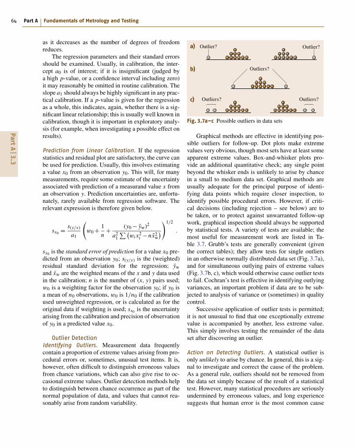
64 Part A Fundamentals of Metrology and Testing
as it decreases as the number of degrees of freedomreduces.
The regression parameters and their standard errorsshould be examined. Usually, in calibration, the inter-cept a0 is of interest; if it is insignificant (judged bya high p-value, or a confidence interval including zero)it may reasonably be omitted in routine calibration. Theslope a1 should always be highly significant in any prac-tical calibration. If a p-value is given for the regressionas a whole, this indicates, again, whether there is a sig-nificant linear relationship; this is usually well known incalibration, though it is important in exploratory analy-sis (for example, when investigating a possible effect onresults).
Prediction from Linear Calibration. If the regressionstatistics and residual plot are satisfactory, the curve canbe used for prediction. Usually, this involves estimatinga value x0 from an observation y0. This will, for manymeasurements, require some estimate of the uncertaintyassociated with prediction of a measurand value x froman observation y. Prediction uncertainties are, unfortu-nately, rarely available from regression software. Therelevant expression is therefore given below.
sx0 =s(y/x)
a1
(w0+ 1
n+ (y0− yw)2
a21
∑(wi x2
i −nx2w
))1/2
.
sx0 is the standard error of prediction for a value x0 pre-dicted from an observation y0; s(y/x) is the (weighted)residual standard deviation for the regression; ywand xw are the weighted means of the x and y data usedin the calibration; n is the number of (x, y) pairs used;w0 is a weighting factor for the observation y0; if y0 isa mean of n0 observations, w0 is 1/n0 if the calibrationused unweighted regression, or is calculated as for theoriginal data if weighting is used; sx0 is the uncertaintyarising from the calibration and precision of observationof y0 in a predicted value x0.
Outlier DetectionIdentifying Outliers. Measurement data frequentlycontain a proportion of extreme values arising from pro-cedural errors or, sometimes, unusual test items. It is,however, often difficult to distinguish erroneous valuesfrom chance variations, which can also give rise to oc-casional extreme values. Outlier detection methods helpto distinguish between chance occurrence as part of thenormal population of data, and values that cannot rea-sonably arise from random variability.
Outlier?a) Outlier?
Outliers?
Outliers? Outliers?
b)
c)
Fig. 3.7a–c Possible outliers in data sets
Graphical methods are effective in identifying pos-sible outliers for follow-up. Dot plots make extremevalues very obvious, though most sets have at least someapparent extreme values. Box-and-whisker plots pro-vide an additional quantitative check; any single pointbeyond the whisker ends is unlikely to arise by chancein a small to medium data set. Graphical methods areusually adequate for the principal purpose of identi-fying data points which require closer inspection, toidentify possible procedural errors. However, if criti-cal decisions (including rejection – see below) are tobe taken, or to protect against unwarranted follow-upwork, graphical inspection should always be supportedby statistical tests. A variety of tests are available; themost useful for measurement work are listed in Ta-ble 3.7. Grubb’s tests are generally convenient (giventhe correct tables); they allow tests for single outliersin an otherwise normally distributed data set (Fig. 3.7a),and for simultaneous outlying pairs of extreme values(Fig. 3.7b, c), which would otherwise cause outlier teststo fail. Cochran’s test is effective in identifying outlyingvariances, an important problem if data are to be sub-jected to analysis of variance or (sometimes) in qualitycontrol.
Successive application of outlier tests is permitted;it is not unusual to find that one exceptionally extremevalue is accompanied by another, less extreme value.This simply involves testing the remainder of the dataset after discovering an outlier.
Action on Detecting Outliers. A statistical outlier isonly unlikely to arise by chance. In general, this is a sig-nal to investigate and correct the cause of the problem.As a general rule, outliers should not be removed fromthe data set simply because of the result of a statisticaltest. However, many statistical procedures are seriouslyundermined by erroneous values, and long experiencesuggests that human error is the most common cause
PartA
3.3

Quality in Measurement and Testing 3.3 Statistical Evaluation of Results 65
Table 3.7 Tests for outliers in normally distributed data. The following assume an ordered set of data x1 . . . xn . Tables ofcritical values for the following can be found in ISO 5725:1995 part 2, among other sources. Symbols otherwise followthose in Table 3.2
Test objective Test name Test statistic Remarks
Test for a single outlier in anotherwise normal distribution
i) Dixon’s test n = 3 . . . 7 :(xn − xn−1)/(xn − x1)n = 8 . . . 10 :(xn − xn−1)/(xn − x2)n = 10 . . . 30 :(xn − xn−2)/(xn − x3)
The test statistics vary with thenumber of data points. Only thetest statistic for a high outlier isshown; to calculate the test statis-tic for a low outlier, renumber thedata in descending order. Criticalvalues must be found from tables ofDixon’s test statistic if not availablein software
ii) Grubb’s test 1 (xn − x)/s (high outlier)(x− x1)/s (low outlier)
Grubb’s test is simpler than Dixon’stest if using software, although crit-ical values must again be foundfrom tables if not available in soft-ware
Test for two outliers on op-posite sides of an otherwisenormal distribution
Grubb’s test 2
1−(
(n−3)[s(x3 . . . xn)]2(n−1)s2
) s(x3 . . . xn) is the standard devia-tion for the data excluding the twosuspected outliers. The test can beperformed on data in both ascend-ing and descending order to detectpaired outliers at each end. Criti-cal values must use the appropriatetables
Test for two outliers on thesame side of an otherwise nor-mal distribution
Grubb’s test 3 (xn − x1)/s Use tables for Grubb’s test 3
Test for a single high variancein l groups of data
Cochran’s test
Cn = (s2)max∑i=1,l
s2i
n = 1
l
∑i=1,l
ni
of extreme outliers. This experience has given rise tosome general rules which are often used in processing,for example, interlaboratory data.
1. Test at the 95% and the 99% confidence level.2. All outliers should be investigated and any errors
corrected.3. Outliers significant at the 99% level may be rejected
unless there is a technical reason to retain them.4. Outliers significant only at the 95% level should
be rejected only if there is an additional, technicalreason to do so.
5. Successive testing and rejection is permitted, but notto the extent of rejecting a large proportion of thedata.
This procedure leads to results which are not un-duly biased by rejection of chance extreme values, butare relatively insensitive to outliers at the frequencycommonly encountered in measurement work. Note,however, that this objective can be attained without out-
lier testing by using robust statistics where appropriate;this is the subject of the next section.
Finally, it is important to remember that an outlier isonly outlying in relation to some prior expectation. Thetests in Table 3.7 assume underlying normality. If thedata were Poisson distributed, for example, too manyhigh values would be rejected as inconsistent with a nor-mal distribution. It is generally unsafe to reject, or eventest for, outliers unless the underlying distribution isknown.
Robust StatisticsIntroduction. Instead of rejecting outliers, robust statis-tics uses methods which are less strongly affected byextreme values. A simple example of a robust estimateof a population mean is the median, which is essen-tially unaffected by the exact value of extreme points.For example, the median of the data set (1, 2, 3, 4, 6)is identical to that of (1, 2, 3, 4, 60). The median, how-ever, is substantially more variable than the mean when
PartA
3.3

66 Part A Fundamentals of Metrology and Testing
the data are not outlier-contaminated. A variety of es-timators have accordingly been developed that retaina useful degree of resistance to outliers without undulyaffecting performance on normally distributed data.A short summary of the main estimators for meansand standard deviations is given below. Robust meth-ods also exist for analysis of variance, linear regression,and other modeling and estimation approaches.
Robust Estimators for Population Means. The me-dian, as noted above, is a relatively robust estimator,widely available in software. It is very resistant to ex-treme values; up to half the data may go to infinitywithout affecting the median value. Another simple ro-bust estimate is the so-called trimmed mean: the meanof the data set with two or more of the most extremevalues removed. Both suffer from increases in variabil-ity for normally distributed data, the trimmed mean lessso.
The mean suffers from outliers in part because itis a least-squares estimate, which effectively gives val-ues a weight related to the square of their distance fromthe mean (that is, the loss function is quadratic). A gen-eral improvement can be obtained using methods whichuse a modified loss function. Huber (see Sect. 3.12 Fur-ther Reading) suggested a number of such estimators,which allocate a weight proportional to squared distanceup to some multiple c of the estimated standard devia-tion s for the set, and thereafter a weight proportionalto distance. Such estimators are called M-estimators, asthey follow from maximum-likelihood considerations.In Huber’s proposal, the algorithm used is to replaceeach value xi in a data set with zi , where
zi =∣∣∣∣∣
xi if X− c × s < xi < X+ c × s
X± c × s otherwise,
and recalculate the mean X, applying the processiteratively until the result converges. A suitable one-dimensional search algorithm may be faster. The esti-mated standard deviation is usually determined usinga separate robust estimator, or (in Huber’s proposal 2)iteratively, together with the mean. Another well-knownapproach is to use Tukey’s biweight as the loss function;this also reduces the weight of extreme observations (tozero, for very extreme values).
Robust Estimators of Standard Deviation. Two com-mon robust estimates of standard deviation are based onrank order statistics, such as the median. The first, themedian absolute deviation (MAD), calculates the me-dian of absolute deviations from the estimated mean
value x, that is, median (|xi − x|). This value is not di-rectly comparable to the standard deviation in the caseof normally distributed data; to obtain an estimate ofthe standard deviation, a modification known as MADeshould be used. This is calculated as MAD/0.6745.Another common estimate is based on the interquar-tile range (IQR) of a set of data; a normal distributionhas standard deviation IQR/1.349. The IQR method isslightly more variable than the MADe method, but isusually easier to implement, as quartiles are frequentlyavailable in software. Huber’s proposal 2 (above) gen-erates a robust estimate of standard deviation as part ofthe procedure; this estimate is expected to be identicalto the usual standard deviation for normally distributeddata. ISO 5725 provides an alternative iterative proce-dure for a robust standard deviation independently ofthe mean.
Using Robust Estimators. Robust estimators can bethought of as providing good estimates of the param-eters for the good data in an outlier-contaminated set.They are appropriate when
• The data are expected to be normally distributed.Here, robust statistics give answers very close toordinary statistics.• The data are expected to be normally distributed,but contaminated with occasional spurious values,which are regarded as unrepresentative or erro-neous. Here, robust estimators are less affected byoccasional extreme values and their use is rec-ommended. Examples include setting up qualitycontrol (QC) charts from real historical data withoccasional errors, and interpreting interlaboratorystudy data with occasional problem observations.
Robust estimators are not recommended where
• The data are expected to follow nonnormal distri-butions, such as binomial, Poisson, chi-squared, etc.These generate extreme values with reasonable like-lihood, and robust estimates based on assumptionsof underlying normality are not appropriate.• Statistics that represent the whole data distribution(including extreme values, outliers, and errors) arerequired.
3.3.4 Statistics for Quality Control
PrinciplesQuality control applies statistical concepts to moni-tor processes, including measurement processes, and
PartA
3.3

Quality in Measurement and Testing 3.3 Statistical Evaluation of Results 67
detect significant departures from normal operation.The general approach to statistical quality control fora measurement process is
1. regularly measure one or more typical test items(control materials),
2. establish the mean and standard deviation of thevalues obtained over time (ignoring any erroneousresults),
3. use these parameters to set up warning and actioncriteria.
The criteria can include checks on stability of the meanvalue and, where measurements on the control materialare replicated, on the precision of the process. It is alsopossible to seek evidence of emerging trends in the data,which might warn of impending or actual problems withthe process.
The criteria can be in the form of, for example, per-mitted ranges for duplicate measurements, or a rangewithin which the mean value for the control materialmust fall. Perhaps the most generally useful implemen-tation, however, is in the form of a control chart. Thefollowing section therefore describes a simple controlchart for monitoring measurement processes.
There is an extensive literature on statistical pro-cess control and control charting in particular, includinga wide range of methods. Some useful references areincluded in Sect. 3.12 Further Reading.
Control ChartingA control chart is a graphical means of monitoringa measurement process, using observations plotted ina time-ordered sequence. Several varieties are in com-mon use, including cusum charts (sensitive to sustainedsmall bias) and range charts, which control precision.The type described here is based on a Shewhart meanchart. To construct the chart
• Obtain the mean x and standard deviation s ofat least 20 observations (averages if replication isused) on a control material. Robust estimates arerecommended for this purpose, but at least ensurethat no erroneous or aberrant results are included inthis preliminary data.• Draw a chart with date as the x-axis, and a y-axiscovering the range approximately x±4s.• Draw the mean as a horizontal line on the chart.Add two warning limits as horizontal lines at x±2s,and two further action limits at x±3s. These limitsare approximate. Exact limits for specific probabil-
ities are provided in, for example, ISO 8258:1991Shewhart control charts.
As further data points are accumulated, plot each newpoint on the chart. An example of such a chart is shownin Fig. 3.8.
Interpreting Control Chart DataTwo rules follow immediately from the action andwarning limits marked on the chart.
• A point outside the action limits is very unlikelyto arise by chance; the process should be regardedas out of control and the reason investigated andcorrected.• A point between the warning and action limits couldhappen occasionally by chance (about 4–5% of thetime). Unless there is additional evidence of lossof control, no action follows. It may be prudent toremeasure the control material.
Other rules follow from unlikely sequences of obser-vations. For example, two points outside the warninglimits – whether on one side or alternate sides – is veryunlikely and should be treated as actionable. A stringof seven or more points above, or below, the mean –whether within the warning limits or not – is unlikelyand may indicate developing bias (some recommenda-tions consider ten such successive points as actionable).Sets of such rules are available in most textbooks onstatistical process control.
Action on Control Chart Action ConditionsIn general, actionable conditions indicate a need for cor-rective action. However, it is prudent to check that thecontrol material measurement is valid before undertak-ing expensive investigations or halting a process. Takinga second control measurement is therefore advised, par-ticularly for warning conditions. However, it is notsensible to continue taking control measurements untilone falls back inside the limits. A single remeasure-ment is sufficient for confirmation of the out-of-controlcondition.
If the results of the second check do not confirm thefirst, it is sensible to ask how best to use the duplicatedata in coming to a final decision. For example, shouldone act on the second observation? Or perhaps take themean of the two results? Strictly, the correct answer re-quires consideration of the precision of the means ofduplicate measurements taken over the appropriate timeinterval. If this is available, the appropriate limits can
PartA
3.3

68 Part A Fundamentals of Metrology and Testing
B0100
019
70
QCL95Mean
(µg/kg)
U95L99
80
90
100
110
120
130
140
150
160
Batch
B0100
384
B0100
756
B0101
120
B0101
608
B0101
881
B0102
022
B0102
085
B0102
153
B0200
207
B0200
457
B0201
732
B0201
824
B0202
025
B0202
111
B0300
185
B0300
372
B0300
807
B0301
135
B0301
629
B0301
997
B0302
314
B0302
385
B0400
118
B0400
468
B0400
638
B0401
698
B0402
079
U99
Fig. 3.8 QC chart example. The figure shows successive QC measurements on a reference material certified for leadcontent. There is evidence of loss of control at points marked by arrows
be calculated from the relevant standard deviation. Ifnot, the following procedure is suggested: First, checkwhether the difference between the two observations isconsistent with the usual operating precision (the resultsshould be within approximately 2.8s of one another). Ifso, take the mean of the two, and compare this with new
limits calculated as x±2s/√
2 and x±3s/√
2 (this isconservative, in that it assumes complete independenceof successive QC measurements; it errs on the side ofaction). If the two results do not agree within the ex-pected precision, the cause requires investigation andcorrection in any case.
3.4 Uncertainty and Accuracy of Measurement and Testing
3.4.1 General Principles
In metrology and testing, the result of a measurementshould always be expressed as the measured quantityvalue together with its uncertainty. The uncertainty ofmeasurement is defined as a nonnegative parametercharacterizing the dispersion of the quantity values be-ing attributed to a measurand [3.17].
Measurement accuracy, which is the closeness ofagreement between a measured quantity value andthe true quantity value of a measurand, is a posi-tive formulation for the fact that the measured value
is deviating from the true value, which is consid-ered unique and, in practise, unknowable. The devi-ation between the measured value and the true valueor a reference value is called the measurement er-ror.
Since the 1990s there has been a conceptual changefrom the traditionally applied error approach to the un-certainty approach.
In the error approach it is the aim of a measure-ment to determine an estimate of the true value that is asclose as possible to that single true value. In the uncer-tainty approach it is assumed that the information from
PartA
3.4

Quality in Measurement and Testing 3.4 Uncertainty and Accuracy of Measurement and Testing 69
measurement only permits assignment of an interval ofreasonable values to the measurand.
The master document, which is acknowledged toapply to all measurement and testing fields and toall types of uncertainties of quantitative results, is theGuide to the Expression of Uncertainty in Measure-ment (GUM) [3.19]. The Joint Committee for Guidesin Metrology Working Group 1 (JCGM-WG1), authorof the GUM, is producing a complementary series ofdocuments to accompany the GUM.
The GUM uncertainty philosophy has already beenintroduced in Chap. 1, its essential points are
• A measurement quantity X, of which the true valueis not known exactly, is considered as a stochasticvariable with a probability function. Often it is as-sumed that this is a normal (Gaussian) distribution.• The result x of a measurement is an estimate of theexpectation value E(X) for X.• The standard uncertainty u(x) of this measuredvalue is equal to the square root of the varianceV (X).• Expectation (quantity value) and variance (standarduncertainty) are estimated either– by statistical processing of repeated measure-
ments (type A uncertainty evaluation) or– by other methods (type B uncertainty evalua-
tion).• The result of a measurement has to be expressedas a quantity value together with its uncertainty, in-cluding the unit of the measurand.
The methodology of measurement evaluation anddetermination of measurement uncertainty are compiled
Type A evaluation:Statistical processing of repeatedmeasurements (e.g., normal distribution)
Type B evaluation:Uncertainties are estimated by othermethods, based on experience or otherinformation.
In cases where a (max – min) interval is known, a probability distribution has to be assumed and the uncertainty can be expressed as shown by the following examples:
Frequency
Measured quantity values xi
• Measured quantity values xi: x1, x2, ..., xn • Rectangular distribution:
• Triangular distribution:
• Arithmetic mean
• Standard deviation
• Standard measurement uncertainty u = s
• Expanded measurement uncertainty: U = k = u
x– = xi
n
i=1
Coverage interval containing p%of measured quantity values(k: coverage factor) k = 2 p = 95 % k = 3 p = 99.7 % ±ks
1n
u =Δ /2
3
s = (xi – x– )2
n
i=1
1n –1
x– = (max + min) / 2
x–
Δ = (max – min)
Δ
u =Δ /2
6
min max
x–min max Fig. 3.9 Principles of measurementevaluation and determination of un-certainty of measurement for a singlemeasurand x
in Fig. 3.9. The statistical evaluation of results has beendescribed in detail in Sect. 3.3.
3.4.2 Practical Example: Accuracy Classesof Measuring Instruments
All measurements of quantity values for single mea-surands as well as for multiple measurands need to beperformed with appropriate measuring instruments, de-vices for making measurements, alone or in conjunctionwith one or more supplementary devices.
The quality of measuring instruments is often de-fined through limits of errors as description of theaccuracy.
Accuracy classes are defined [3.17] as classes ofmeasuring instruments or measuring systems that meetstated metrological requirements that are intended tokeep measurement errors or instrumental measurementuncertainties within specified limits under specified op-erating conditions. An accuracy class is usually denotedby a number or symbol adopted by convention. Ana-log measuring instruments are divided conventionallyinto accuracy classes of 0.05, 0.1, 0.2, 0.3, 0.5, 1,1.5, 2, 2.5, 3, and 5. The accuracy classes p repre-sent the maximum permissible relative measurementerror in %. For example an accuracy class of 1.0 in-dicates that the limits of error – in both directions –should not exceed 1% of the full-scale deflection. Indigital instruments, the limit of indication error is ±1of the least significant unit of the digital indicationdisplay.
In measuring instruments with an analog indication,the measured quantity is determined by the position
PartA
3.4

70 Part A Fundamentals of Metrology and Testing
Measurement uncertainty of a single measurand with a single measuring instrumentExample from dimensional metrology
(1) Calibration of measuring instrument (measurand: length)
(2) Measurement
Measurement object,e.g., steel rod
Reference: gage block (traceable to the Si length unit with an optical interferometer)
Calibration diagram of themeasuring instrument
The strip Δ is the range of themaximum permissible measurement errors of a measuring instrument with an accuracy classp = (Δ/(2ymax)) · 100 [%].From Δ or p, the instrumentmeasurement uncertainty uinstr. can be estimated in a type B evaluation. Assuming a rectangular distribution(Fig. 3.9) it follows thatuinstr. = (Δ/2) 3, oruinstr. = ((p/100) · ymax) / 3.The relative instrumentmeasurement uncertainty [%]δinstr. = uinstr. /umax is given byδinstr. = p / 3.
Measurement result:Quantity value x
± instrument measurementuncertainty uinstr.
Measuring instrument
Referencevalue r
Accuracyclass p Indication y
Indication y
Accuracyclass p
Indicationlimits
r
y ymax
Indication
Ref
eren
ce v
alue
sof
the
mea
sura
nd Δ
x
max
min
IndicationM
easu
rem
ent r
esul
t
y
Δ
Fig. 3.10 Method for obtaining a measurement result and estimating the instrument measurement uncertainty
of the indicator on the scale. The limits of errors(percentages) are usually given at the full-scale ampli-tude (maximum value of measurement range). Fromthe accuracy class p, also the instrumental measure-ment uncertainty uinstr can be estimated. In Fig. 3.10,the method for obtaining a measurement result andmeasurement uncertainty for a single measurand witha single measuring instrument is shown.
As illustrated in Fig. 3.10, a measuring instrumentgives as output an indication, which has to be relatedto the quantity value of the measurand through a cal-ibration diagram. A calibration diagram represents therelation between indications of a measuring instrumentand a set of reference values of the measurand. Atthe maximum indication value (maximum measurementrange) ymax the width Δ of the strip of the calibra-tion diagram is the range of the maximum permissiblemeasurement errors.
From the determination of Δ the accuracy class pin % follows as
p =(
Δ
(2ymax)
)·100 [%] .
Note that, at indicator amplitudes lower than the max-imum ymax, the actual relative maximum permissiblemeasurement errors pact for the position yact on thescale need to be determined as
pact = p ·(
ymax
yact
).
For the estimation of the standard measurement uncer-tainty it can be considered in an uncertainty estimationof type B that all values in the range between the limitsof indications have the same probability – as long as noother information is available. This kind of distributionis called a rectangular distribution (Fig. 3.9). Therefore,the standard uncertainty is equal to
uinstr = (Δ/2)√3
= ((p/100) · ymax)√3
.
Example 3.1: What is the measurement uncertainty ofa measurement result obtained by a measurement withan analog voltmeter (accuracy class 2.0) with a max-imum amplitude of 380 V, when the indicator is at220 V?
PartA
3.4

Quality in Measurement and Testing 3.4 Uncertainty and Accuracy of Measurement and Testing 71
(Σpi2 )
uSystem/ |y| =
uSystem/ |y| =
Measurement uncertainty of a measurement system or measurement chain
Consider a measurement system, consisting in the simplest case of three components,namely a sensor (accuracy class pS), an amplifier (accuracy class pA) and a display(accuracy class D3)
The measurement uncertainty of the system can be estimated by applying the law of thepropagation of uncertainties (see Sect. 3.4.3)
It follows that
Quantity to bemeasured x
Sensor pS
Amplifier pA
Display pD
Outputy
Electricalsignal
(pS2 + pA
2 + pD2)
(uS2/xS
2 + uA2/xA
2 + uD2 /xD
2),
δchain = uchain /|y| = (i = 1…n)3
where uS /xS + uA/xA, uD/xD, are the relative instrumentuncertainties of sensor, amplifier and display, which can beexpressed by their accuracy classes as pS/ 3, pA/ 3, pD/ 3.
3
For a measurement system of n components in line, the following formula characterizes the relative uncertainty budget of the measuring chain
Fig. 3.11 Method for estimating themeasurement system uncertainty
Consideration: actual relative maximum permissi-ble measurement errors for 220 V and limits of errorexpressed in measurement units (V as scale divisions)are
p220,rel = 2.0% · 380 V
220 V= 3.5% ;
pabs = 380 V · 2.0%
100%= 7.6 V (limits of error)
uinstr,rel = prel√3= 3.5%√
3= 2.0% and
uinstr,abs = pabs√3= 7.6 V√
3= 4.4 V .
It is obvious that the relative standard uncertaintiesare smallest at ymax.
Since a rectangular distribution was assumed, it isnot reasonable to apply the coverage factor k, becausethis approach assumes a Gaussian distribution. Instead,the standard uncertainty uinstr should be stated. It nor-mally suffices to report the uncertainties to at most twosignificant digits – and also to provide information onhow it was determined. Finally, the measurement un-certainty allows the experimenter to decide whether theused instrument is appropriate for his/the customer’sneeds.
Answer: The result of the example could be reportedas 220 V±4.4 V. The measurement uncertainty of the
instrument is reported as a standard uncertainty (cover-age factor k = 1) and was obtained by type B evaluationonly considering the instrument accuracy class.
If instead of a single measuring instrument, a meas-uring system or a measuring chain is used, consistingin the simplest case of a sensor, an amplifier, anda display, the accuracy classes of the components ofthe measuring system can also be used to estimatethe instrumental system uncertainty, as illustrated inFig. 3.11.
3.4.3 Multiple Measurement UncertaintyComponents
The method outlined in Figs. 3.9 and 3.10 consid-ers only one single measurement quantity and onlythe sources covered by only one variable. However,very often uncertainty evaluations have to be relatedto functional combinations of measured quantities oruncertainty components y = f (x1, x2, x3, . . ., xn). Inthese cases, for uncorrelated (i. e., independent) values,the single uncertainties are combined by applying thelaw of propagation of uncertainty to give the so-calledcombined measurement uncertainty
ucombined(y) =√∑(
∂ f
∂xi
)2
u2(xi ) .
PartA
3.4