springer series in statistics - download.e-bookshelf.de · brockwell/davis: time series: theory and...

Springer Series in Statistics

Advisors:P. Bickel, P. Diggle, S. Fienberg, U. Gather,I. Olkin, S. Zeger

Springer Series in StatisticsAlho/Spencer: Statistical Demography and Forecasting.Andersen/Borgan/Gill/Keiding: Statistical Models Based on Counting Processes.Atkinson/Riani: Robust Diagnostic Regression Analysis.Atkinson/Riani/Ceriloi: Exploring Multivariate Data with the Forward Search.Berger: Statistical Decision Theory and Bayesian Analysis, 2nd edition.Borg/Groenen: Modern Multidimensional Scaling: Theory and Applications,

2nd edition.Brockwell/Davis: Time Series: Theory and Methods, 2nd edition.Bucklew: Introduction to Rare Event Simulation.Cappé/Moulines/Rydén: Inference in Hidden Markov Models.Chan/Tong: Chaos: A Statistical Perspective.Chen/Shao/Ibrahim: Monte Carlo Methods in Bayesian Computation.Coles: An Introduction to Statistical Modeling of Extreme Values.Devroye/Lugosi: Combinatorial Methods in Density Estimation.Diggle/Ribeiro: Model-based Geostatistics.Efromovich: Nonparametric Curve Estimation: Methods, Theory, and Applications.Eggermont/LaRiccia: Maximum Penalized Likelihood Estimation, Volume I:

Density Estimation.Fahrmeir/Tutz: Multivariate Statistical Modeling Based on Generalized Linear

Models, 2nd edition.Fan/Yao: Nonlinear Time Series: Nonparametric and Parametric Methods.Ferraty/Vieu: Nonparametric Functional Data Analysis: Theory and Practice.Fienberg/Hoaglin: Selected Papers of Frederick Mosteller.Frühwirth-Schnatter: Finite Mixture and Markov Switching Models.Ghosh/Ramamoorthi: Bayesian Nonparametrics.Glaz/Naus/Wallenstein: Scan Statistics.Good: Permutation Tests: Parametric and Bootstrap Tests of Hypotheses,

3rd edition.Gouriéroux: ARCH Models and Financial Applications.Gu: Smoothing Spline ANOVA Models.Gyöfi/Kohler/Krzyzak/Walk: A Distribution-Free Theory of Nonparametric

Regression.Haberman: Advanced Statistics, Volume I: Description of Populations.Hall: The Bootstrap and Edgeworth Expansion.Härdle: Smoothing Techniques: With Implementation in S.Harrell: Regression Modeling Strategies: With Applications to Linear Models,

Logistic Regression, and Survival Analysis.Hart: Nonparametric Smoothing and Lack-of-Fit Tests.Hastie/Tibshirani/Friedman: The Elements of Statistical Learning: Data Mining,

Inference, and Prediction.Hedayat/Sloane/Stufken: Orthogonal Arrays: Theory and Applications.Heyde: Quasi-Likelihood and its Application: A General Approach to Optimal

Parameter Estimation.Huet/Bouvier/Poursat/Jolivet: Statistical Tools for Nonlinear Regression:

A Practical Guide with S-PLUS and R Examples, 2nd edition.Ibrahim/Chen/Sinha: Bayesian Survival Analysis.Jiang: Linear and Generalized Linear Mixed Models and Their Applications.Jolliffe: Principal Component Analysis, 2nd edition.Knottnerus: Sample Survey Theory: Some Pythagorean Perspectives.Küchler/Sørensen: Exponential Families of Stochastic Processes.Kutoyants: Statistical Inference for Ergodic Diffusion Processes.

(continued after index)

Jiming Jiang

Linear and Generalized Linear Mixed Models and Their Applications

Library of Congress Control Number: 2006935876

ISBN-10: 0-387-47941-4 e-ISBN-10: 0-387-47946-5ISBN-13: 978-0-387-47941-5 e-ISBN-13: 978-0-387-47946-0

Printed on acid-free paper.

© 2007 Springer Science +Business Media, LLCAll rights reserved. This work may not be translated or copied in whole or in part without thewritten permission of the publisher (Springer Science+Business Media, LLC, 233 Spring Street,New York, NY 10013, USA), except for brief excerpts in connection with reviews or scholarlyanalysis. Use in connection with any form of information storage and retrieval, electronic adaptation, computer software, or by similar or dissimilar methodology now known or hereafterdeveloped is forbidden.The use in this publication of trade names, trademarks, service marks, and similar terms, even ifthey are not identified as such, is not to be taken as an expression of opinion as to whether ornot they are subject to proprietary rights.

9 8 7 6 5 4 3 2 1

springer.com

Jiming JiangDepartment of StatisticsUniversity of California, DavisDavis, CA [email protected]

To my children

Preface

Over the past decade there has been an explosion of developments in mixedeffects models and their applications. This book concentrates on two majorclasses of mixed effects models, linear mixed models and generalized linearmixed models, with the intention of offering an up-to-date account of theoryand methods in the analysis of these models as well as their applications invarious fields.

The first two chapters are devoted to linear mixed models. We classify lin-ear mixed models as Gaussian (linear) mixed models and non-Gaussian linearmixed models. There have been extensive studies in estimation in Gaussianmixed models as well as tests and confidence intervals. On the other hand,the literature on non-Gaussian linear mixed models is much less extensive,partially because of the difficulties in inference about these models. However,non-Gaussian linear mixed models are important because, in practice, one isnever certain that normality holds. This book offers a systematic approachto inference about non-Gaussian linear mixed models. In particular, it hasincluded recently developed methods, such as partially observed information,iterative weighted least squares, and jackknife in the context of mixed models.Other new methods introduced in this book include goodness-of-fit tests, pre-diction intervals, and mixed model selection. These are, of course, in additionto traditional topics such as maximum likelihood and restricted maximumlikelihood in Gaussian mixed models.

The next two chapters deal with generalized linear mixed models. Thesemodels may be regarded as extensions of the Gaussian mixed models. They areuseful in situations where responses are correlated as well as discrete or cate-gorical. McCullagh and Nelder (1989) introduced one of the earlier examplesof such models, a mixed logistic model, for the infamous salamander matingproblem. Since then these models have received considerable attention, andvarious methods of inference have been developed. A major issue regardinggeneralized linear mixed models is the computation of the maximum likeli-hood estimator. It is known that the likelihood function under these modelsmay involve high-dimensional integrals that cannot be evaluated analytically.

VIII Preface

Therefore, the maximum likelihood estimator is difficult to compute. We clas-sify the methods of inference as likelihood-based, which include the Bayesianmethods, and nonlikelihood-based. The likelihood-based approaches focus ondeveloping computational methods. Markov chain Monte Carlo methods havebeen used in both the likelihood and the Bayesian approaches to handle thecomputations. The nonlikelihood-based approaches try to avoid the compu-tational difficulty by considering alternative methods. These include approxi-mate inference and estimating equations. Another challenging problem in thisarea is generalized linear mixed model selection. A recently developed method,called fence, is shown to be applicable to selecting an optimal model from aset of candidate models.

There have been various books on mixed effects models and related topics.The following are the major ones published in the last ten years.

1. Demidenko (2004), Mixed Models—Theory and Applications2. McCulloch and Searle (2001), Generalized, Linear and Mixed Models3. Sahai and Ageel (2000), Analysis of Variance: Fixed, Random and MixedModels4. Verbeke et al. (2000), Linear Mixed Models for Longitudinal Data5. Pinheiro and Bates (2000), Mixed-Effects Models in S and S-Plus6. Brown and Prescott (1999), Applied Mixed Models in Medicine7. Rao (1997), Variance Components Estimation: Mixed Models, Methodolo-gies and Applications8. Littell et al. (1996), SAS System for Mixed Models

The latest publication, book 1, provides a quite comprehensive introductionon Gaussian mixed models and applications in problems such as tumor re-growth, shape, and image. Book 2 emphasizes application of the maximumlikelihood and restricted maximum likelihood methods for estimation. Book3 intensively studies the ANOVA type models with examples and computerprograms using statistical software packages. Books 4, 5, 6 and 8 are mainlyapplication-oriented. Many examples and case studies are available, and com-puter programs in SAS and S-Plus as well. Book 7 presents a comprehensiveaccount of the major procedures of estimating the variance components, andfixed and random effects. These books, however, do not discuss non-Gaussianlinear mixed models, neither do they present model diagnostics and model se-lection methods for mixed models. As mentioned, non-Gaussian linear mixedmodels, mixed model diagnostics, and mixed model selection are among themain topics of this book.

The application of mixed models is vast and expanding so fast as to pre-clude any attempt at exhaustive coverage. Here we use a number of selectedreal-data examples to illustrate the applications of linear and generalized lin-ear mixed models. The areas of application include biological and medicalresearch, animal and human genetics, and small area estimation. The lat-ter has evolved quite rapidly in surveys. These examples of applications areconsidered near the end of each chapter.

Preface IX

The text is supplemented by numerous exercises. The majority of the prob-lems are related to the subjects discussed in each chapter. In addition, somefurther results and technical notes are given in the last section of each chap-ter. The bibliography includes the relevant references. Three appendices areattached. Appendix A lists the notation used in this book. Appendix B pro-vides the necessary background in matrix algebra. Appendix C gives a briefreview of some of the relevant results in probability and statistics.

The book is aimed at students, researchers, and other practitioners whoare interested in using mixed models for statistical data analysis or doingresearch in this area. The book is suitable for a course in a MS program instatistics, provided that the sections of further results and technical notes areskipped. If the latter sections are included, the book may be used for twocourses in a PhD program in statistics, perhaps one on linear models and theother on generalized linear models, both with applications. A first course inmathematical statistics, the ability to use a computer for data analysis andfamiliarity with calculus and linear algebra are prerequisites. Additional sta-tistical courses, such as regression analysis, and a good knowledge of matriceswould be helpful.

A large portion of the material in this book is based on lecture notes fromtwo graduate courses, “Linear Models” and “Generalized Linear Models”, thatthe author taught at Case Western Reserve University between 1996 and 2001.The author would like to thank Prof. Joe Sedransk for initiating these courses.Grateful thanks are also due, in particular, to Prof. Partha Lahiri for his rolein drawing the author’s attention to application of mixed models to small areaestimation, and to Prof. Rudy Beran for his advice and encouragement. Myspecial thanks also go to Prof. J. N. K. Rao, who reviewed an earlier version ofthis book and made valuable suggestions. A number of anonymous reviewershave reviewed the earlier drafts of this book, or chapters of this book. Theircomments led to major changes, especially in the organization of the contents.The author wishes to thank them for their time and effort that have madethe book suitable for a broader audience. Two graduate students have helpedwith the data analyses that are involved in this book. In this regard, mysincere thanks go to Ms. Zhonghua Gu and Ms. Thuan Nguyen. In addition,the author thanks Ms. Qiuyan Xu and Ms. Zhonghua Gu for proofreading thebook and providing solutions to some of the exercises. Finally, the author isgrateful for Dr. Sean M. D. Allan for his comments that helped improve thepresentation of this preface.

Jiming JiangDavis, CaliforniaJuly, 2006

Contents

Preface . . . . . . . . . . . . . . . . . . . . . . . . . . . . . . . . . . . . . . . . . . . . . . . . . . . . . . . . VII

1 Linear Mixed Models: Part I . . . . . . . . . . . . . . . . . . . . . . . . . . . . . . 11.1 Introduction . . . . . . . . . . . . . . . . . . . . . . . . . . . . . . . . . . . . . . . . . . . . 1

1.1.1 Effect of Air Pollution Episodes on Children . . . . . . . . . . 21.1.2 Prediction of Maize Single-Cross Performance . . . . . . . . . 31.1.3 Small Area Estimation of Income . . . . . . . . . . . . . . . . . . . . 3

1.2 Types of Linear Mixed Models . . . . . . . . . . . . . . . . . . . . . . . . . . . . 41.2.1 Gaussian Mixed Models . . . . . . . . . . . . . . . . . . . . . . . . . . . . 41.2.2 Non-Gaussian Linear Mixed Models . . . . . . . . . . . . . . . . . 8

1.3 Estimation in Gaussian Models . . . . . . . . . . . . . . . . . . . . . . . . . . . . 91.3.1 Maximum Likelihood . . . . . . . . . . . . . . . . . . . . . . . . . . . . . . 91.3.2 Restricted Maximum Likelihood . . . . . . . . . . . . . . . . . . . . . 12

1.4 Estimation in Non-Gaussian Models . . . . . . . . . . . . . . . . . . . . . . . 151.4.1 Quasi-Likelihood Method . . . . . . . . . . . . . . . . . . . . . . . . . . . 161.4.2 Partially Observed Information. . . . . . . . . . . . . . . . . . . . . . 181.4.3 Iterative Weighted Least Squares . . . . . . . . . . . . . . . . . . . . 201.4.4 Jackknife Method . . . . . . . . . . . . . . . . . . . . . . . . . . . . . . . . . 24

1.5 Other Methods of Estimation . . . . . . . . . . . . . . . . . . . . . . . . . . . . . 251.5.1 Analysis of Variance Estimation . . . . . . . . . . . . . . . . . . . . . 251.5.2 Minimum Norm Quadratic Unbiased Estimation . . . . . . 28

1.6 Notes on Computation and Software . . . . . . . . . . . . . . . . . . . . . . . 291.6.1 Notes on Computation . . . . . . . . . . . . . . . . . . . . . . . . . . . . . 291.6.2 Notes on Software . . . . . . . . . . . . . . . . . . . . . . . . . . . . . . . . . 33

1.7 Real-Life Data Examples . . . . . . . . . . . . . . . . . . . . . . . . . . . . . . . . . 341.7.1 Analysis of Birth Weights of Lambs . . . . . . . . . . . . . . . . . . 351.7.2 Analysis of Hip Replacements Data . . . . . . . . . . . . . . . . . . 37

1.8 Further Results and Technical Notes . . . . . . . . . . . . . . . . . . . . . . . 391.9 Exercises . . . . . . . . . . . . . . . . . . . . . . . . . . . . . . . . . . . . . . . . . . . . . . . 48

XII Contents

2 Linear Mixed Models: Part II . . . . . . . . . . . . . . . . . . . . . . . . . . . . . 512.1 Tests in Linear Mixed Models . . . . . . . . . . . . . . . . . . . . . . . . . . . . . 51

2.1.1 Tests in Gaussian Mixed Models . . . . . . . . . . . . . . . . . . . . 512.1.2 Tests in Non-Gaussian Linear Mixed Models . . . . . . . . . . 56

2.2 Confidence Intervals in Linear Mixed Models . . . . . . . . . . . . . . . . 662.2.1 Confidence Intervals in Gaussian Mixed Models . . . . . . . 662.2.2 Confidence Intervals in Non-Gaussian Linear Mixed

Models . . . . . . . . . . . . . . . . . . . . . . . . . . . . . . . . . . . . . . . . . . . 722.3 Prediction . . . . . . . . . . . . . . . . . . . . . . . . . . . . . . . . . . . . . . . . . . . . . . 74

2.3.1 Prediction of Mixed Effect . . . . . . . . . . . . . . . . . . . . . . . . . . 742.3.2 Prediction of Future Observation . . . . . . . . . . . . . . . . . . . . 80

2.4 Model Checking and Selection . . . . . . . . . . . . . . . . . . . . . . . . . . . . . 882.4.1 Model Diagnostics . . . . . . . . . . . . . . . . . . . . . . . . . . . . . . . . . 882.4.2 Model Selection . . . . . . . . . . . . . . . . . . . . . . . . . . . . . . . . . . . 93

2.5 Bayesian Inference . . . . . . . . . . . . . . . . . . . . . . . . . . . . . . . . . . . . . . . 992.5.1 Inference about Variance Components . . . . . . . . . . . . . . . 1002.5.2 Inference about Fixed and Random Effects . . . . . . . . . . . 101

2.6 Real-Life Data Examples . . . . . . . . . . . . . . . . . . . . . . . . . . . . . . . . . 1022.6.1 Analysis of the Birth Weights of Lambs (Continued) . . . 1022.6.2 The Baseball Example . . . . . . . . . . . . . . . . . . . . . . . . . . . . . 103

2.7 Further Results and Technical Notes . . . . . . . . . . . . . . . . . . . . . . . 1052.8 Exercises . . . . . . . . . . . . . . . . . . . . . . . . . . . . . . . . . . . . . . . . . . . . . . . 113

3 Generalized Linear Mixed Models: Part I . . . . . . . . . . . . . . . . . . 1193.1 Introduction . . . . . . . . . . . . . . . . . . . . . . . . . . . . . . . . . . . . . . . . . . . . 1193.2 Generalized Linear Mixed Models . . . . . . . . . . . . . . . . . . . . . . . . . 1203.3 Real-Life Data Examples . . . . . . . . . . . . . . . . . . . . . . . . . . . . . . . . . 122

3.3.1 The Salamander Mating Experiments . . . . . . . . . . . . . . . . 1223.3.2 A Log-Linear Mixed Model for Seizure Counts . . . . . . . . 1243.3.3 Small Area Estimation of Mammography Rates . . . . . . . 124

3.4 Likelihood Function under GLMM . . . . . . . . . . . . . . . . . . . . . . . . . 1253.5 Approximate Inference . . . . . . . . . . . . . . . . . . . . . . . . . . . . . . . . . . . 127

3.5.1 Laplace Approximation . . . . . . . . . . . . . . . . . . . . . . . . . . . . 1273.5.2 Penalized Quasi-Likelihood Estimation . . . . . . . . . . . . . . . 1283.5.3 Tests of Zero Variance Components . . . . . . . . . . . . . . . . . . 1323.5.4 Maximum Hierarchical Likelihood . . . . . . . . . . . . . . . . . . . 134

3.6 Prediction of Random Effects . . . . . . . . . . . . . . . . . . . . . . . . . . . . . 1363.6.1 Joint Estimation of Fixed and Random Effects . . . . . . . . 1363.6.2 Empirical Best Prediction . . . . . . . . . . . . . . . . . . . . . . . . . . 1423.6.3 A Simulated Example . . . . . . . . . . . . . . . . . . . . . . . . . . . . . . 149

3.7 Further Results and Technical Notes . . . . . . . . . . . . . . . . . . . . . . . 1513.7.1 More on NLGSA . . . . . . . . . . . . . . . . . . . . . . . . . . . . . . . . . . 1513.7.2 Asymptotic Properties of PQWLS Estimators . . . . . . . . . 1523.7.3 MSE of EBP. . . . . . . . . . . . . . . . . . . . . . . . . . . . . . . . . . . . . . 1553.7.4 MSPE of the Model-Assisted EBP . . . . . . . . . . . . . . . . . . . 158

Contents XIII

3.8 Exercises . . . . . . . . . . . . . . . . . . . . . . . . . . . . . . . . . . . . . . . . . . . . . . . 161

4 Generalized Linear Mixed Models: Part II . . . . . . . . . . . . . . . . . 1634.1 Likelihood-Based Inference . . . . . . . . . . . . . . . . . . . . . . . . . . . . . . . 163

4.1.1 A Monte Carlo EM Algorithm for Binary Data . . . . . . . . 1644.1.2 Extensions . . . . . . . . . . . . . . . . . . . . . . . . . . . . . . . . . . . . . . . 1674.1.3 MCEM with I.I.D. Sampling . . . . . . . . . . . . . . . . . . . . . . . . 1704.1.4 Automation . . . . . . . . . . . . . . . . . . . . . . . . . . . . . . . . . . . . . . 1714.1.5 Maximization by Parts . . . . . . . . . . . . . . . . . . . . . . . . . . . . . 1744.1.6 Bayesian Inference . . . . . . . . . . . . . . . . . . . . . . . . . . . . . . . . . 178

4.2 Estimating Equations . . . . . . . . . . . . . . . . . . . . . . . . . . . . . . . . . . . . 1834.2.1 Generalized Estimating Equations (GEE) . . . . . . . . . . . . 1844.2.2 Iterative Estimating Equations . . . . . . . . . . . . . . . . . . . . . . 1864.2.3 Method of Simulated Moments . . . . . . . . . . . . . . . . . . . . . . 1904.2.4 Robust Estimation in GLMM . . . . . . . . . . . . . . . . . . . . . . . 196

4.3 GLMM Selection . . . . . . . . . . . . . . . . . . . . . . . . . . . . . . . . . . . . . . . . 1994.3.1 A General Principle for Model Selection . . . . . . . . . . . . . . 2004.3.2 A Simulated Example . . . . . . . . . . . . . . . . . . . . . . . . . . . . . . 203

4.4 Real-Life Data Examples . . . . . . . . . . . . . . . . . . . . . . . . . . . . . . . . . 2054.4.1 Fetal Mortality in Mouse Litters . . . . . . . . . . . . . . . . . . . . 2054.4.2 Analysis of Gc Genotype Data: An Application of the

Fence Method . . . . . . . . . . . . . . . . . . . . . . . . . . . . . . . . . . . . . 2074.4.3 The Salamander-Mating Experiments: Various

Applications of GLMM. . . . . . . . . . . . . . . . . . . . . . . . . . . . . 2094.5 Further Results and Technical Notes . . . . . . . . . . . . . . . . . . . . . . . 214

4.5.1 Proof of Theorem 4.3 . . . . . . . . . . . . . . . . . . . . . . . . . . . . . . 2144.5.2 Linear Convergence and Asymptotic Properties

of IEE . . . . . . . . . . . . . . . . . . . . . . . . . . . . . . . . . . . . . . . . . . . 2144.5.3 Incorporating Informative Missing Data in IEE . . . . . . . 2174.5.4 Consistency of MSM Estimator . . . . . . . . . . . . . . . . . . . . . 2184.5.5 Asymptotic Properties of First and

Second-Step Estimators . . . . . . . . . . . . . . . . . . . . . . . . . . . . 2214.5.6 Further Results of the Fence Method. . . . . . . . . . . . . . . . . 225

4.6 Exercises . . . . . . . . . . . . . . . . . . . . . . . . . . . . . . . . . . . . . . . . . . . . . . . 229. . . . . . . . . . . . . . . . . . . . . . . . . . . . . . . . . . . . . . . . . . . . . . . . . . . . . . . . . . . 230

A List of Notations . . . . . . . . . . . . . . . . . . . . . . . . . . . . . . . . . . . . . . . . . . 231

B Matrix Algebra . . . . . . . . . . . . . . . . . . . . . . . . . . . . . . . . . . . . . . . . . . . . 233B.1 Kronecker Products . . . . . . . . . . . . . . . . . . . . . . . . . . . . . . . . . . . . . . 233B.2 Matrix Differentiation . . . . . . . . . . . . . . . . . . . . . . . . . . . . . . . . . . . . 233B.3 Projection . . . . . . . . . . . . . . . . . . . . . . . . . . . . . . . . . . . . . . . . . . . . . . 234B.4 Generalized Inverse . . . . . . . . . . . . . . . . . . . . . . . . . . . . . . . . . . . . . . 235B.5 Decompositions of Matrices . . . . . . . . . . . . . . . . . . . . . . . . . . . . . . . 235B.6 The Eigenvalue Perturbation Theory . . . . . . . . . . . . . . . . . . . . . . . 236

XIV Contents

C Some Results in Statistics . . . . . . . . . . . . . . . . . . . . . . . . . . . . . . . . . 237C.1 Multivariate Normal Distribution . . . . . . . . . . . . . . . . . . . . . . . . . . 237C.2 Quadratic Forms . . . . . . . . . . . . . . . . . . . . . . . . . . . . . . . . . . . . . . . . 237C.3 OP and oP . . . . . . . . . . . . . . . . . . . . . . . . . . . . . . . . . . . . . . . . . . . . . . 238C.4 Convolution . . . . . . . . . . . . . . . . . . . . . . . . . . . . . . . . . . . . . . . . . . . . 238C.5 Exponential Family and Generalized Linear Models . . . . . . . . . . 239

References . . . . . . . . . . . . . . . . . . . . . . . . . . . . . . . . . . . . . . . . . . . . . . . . . . . . . 241

Index . . . . . . . . . . . . . . . . . . . . . . . . . . . . . . . . . . . . . . . . . . . . . . . . . . . . . . . . . . 255

1

Linear Mixed Models: Part I

1.1 Introduction

The best way to understand a linear mixed model, or mixed linear model insome earlier literature, is to first recall a linear regression model. The lattercan be expressed as y = Xβ + ε, where y is a vector of observations, X is amatrix of known covariates, β is a vector of unknown regression coefficients,and ε is a vector of (unobservable random) errors. In this model, the regressioncoefficients are considered fixed. However, there are cases in which it makessense to assume that some of these coefficients are random. These cases typ-ically occur when the observations are correlated. For example, in medicalstudies observations are often collected from the same individuals over time.It may be reasonable to assume that correlations exist among the observationsfrom the same individual, especially if the times at which the observations arecollected are relatively close. In animal breeding, lactation yields of dairy cowsassociated with the same sire may be correlated. In educational research, testscores of the same student may be related.

Now, let us see how a linear mixed model may be useful for modelingthe correlations among the observations. Consider, for example, the exampleabove regarding medical studies. Assume that each individual is associatedwith a random effect whose value is unobservable. Let yij denote the obser-vation from the ith individual collected at time tj , and αi the random effectassociated with the ith individual. Assume that there are m individuals. Forsimplicity, let us assume that the observations from all individuals are col-lected at a common set of times, say, t1, . . . , tk. Then, a linear mixed modelmay be expressed as yij = x′

ijβ + αi + εij , i = 1, . . . , m, j = 1, . . . , k, wherexij is a vector of known covariates; β is a vector of unknown regression co-efficients; the random effects α1, . . . , αm are assumed to be i.i.d. with meanzero and variance σ2; the εijs are errors that are i.i.d. with mean zero andvariance τ2; and the random effects and errors are independent. It followsthat the correlation between any two observations from the same individualis σ2/(σ2 + τ2), whereas observations from different individuals are uncorre-

2 1 Linear Mixed Models: Part I

lated. This model is a special case of the so-called longitudinal linear mixedmodel, which is discussed in much detail in the sequel. Of course, this is onlya simple model and it may not capture all the correlations among the obser-vations. Therefore, we would like to have a richer class of models that allowsfurther complications.

A general linear mixed model may be expressed as

y = Xβ + Zα + ε, (1.1)

where y is a vector of observations, X is a matrix of known covariates, β isa vector of unknown regression coefficients, which are often called the fixedeffects, Z is a known matrix, α is a vector of random effects, and ε is a vectorof errors. Both α and ε are unobservable. Compared with the linear regressionmodel, it is clear that the difference is Zα, which may take many differentforms, thus creating a rich class of models, as we shall see. A statistical modelmust come with assumptions. The basic assumptions for (1.1) are that therandom effects and errors have mean zero and finite variances. Typically,the covariance matrices G = Var(α) and R = Var(ε) involve some unknowndispersion parameters, or variance components. It is also assumed that α andε are uncorrelated.

We conclude this section with three examples illustrating the applicationsof linear mixed models, with more examples to come later.

1.1.1 Effect of Air Pollution Episodes on Children

Laird and Ware (1982) discussed an example of analysis of the effect of airpollution episodes on pulmonary function. About 200 school children wereexamined under normal conditions, then during an air pollution alert, andon three successive weeks following the alert. One of the objectives was todetermine whether the volume of air exhaled in the first second of a forcedexhalation, denoted by FEV1, was depressed during the alert.

Note that in this case the data were longitudinally collected with fiveobservational times common for all the children. Laird and Ware proposedthe following simple linear mixed model for analysis of the longitudinal data:yij = βj + αi + εij , i = 1, . . . , m, j = 1, . . . , 5, where βj is the mean FEV1 forthe jth observational time, αi is a random effect associated with the ith child,εij is an error term, and m is the total number of children. It is assumed thatthe random effects are independent and distributed as N(0, τ2), the errors areindependent and distributed as N(0, σ2), and the random effects and errors areindependent. It should be mentioned that some measurements were missingin this study. However, the above model can be modified to take this intoaccount. In particular, the number of observations for the ith individual maybe denoted by ni, where 1 ≤ ni ≤ 5.

Based on the model, Laird and Ware were able to analyze the data usingmethods described in the sequel, with the following findings: (i) a decline in

1.1 Introduction 3

mean FEV1 was observed on and after the alert day; and (ii) the variances andcovariances for the last four measurements were larger than those involvingthe baseline day. The two authors further studied the problem of identificationof sensitive subgroups or individuals most severely affected by the pollutionepisode using a more complicated linear mixed model.

1.1.2 Prediction of Maize Single-Cross Performance

Bernardo (1996) reported results of best linear unbiased prediction, or BLUP,of single-cross performance using a linear mixed model and genetic relation-ship among parental inbreds. Grain yield, moisture, stalk lodging and rootlodging data were obtained for 2043 maize single crosses evaluated in themultilocation testing program of Limagrain Genetics, from 1990 to 1994. Theobjective of the study was to investigate the robustness of BLUP for iden-tifying superior single crosses when estimates of genetic relationship amonginbreds are erroneous.

In analysis of the single-cross data, Bernardo proposed the following linearmixed model: y = Xβ + Z0c + Z1g1 + Z2g2 + Zd + e, where y is a vectorof observed performance for a given trait (i.e., hybrid by multilocation trialmeans); β is a vector of fixed effects of multilocation yield trials; c is a vectorof check effects; gj is a vector of general combining ability effects of groupj, j = 1, 2; d is a vector of specific combining ability effects; e is a vector ofresidual effects; and X, Zj , j = 0, 1, 2 and Z are (known) incidence matricesof 0s and 1s. Here c, g1, g2, and d are treated as random effects. It is assumedthat c, g1, g2, d, and e are uncorrelated with their covariance matrices modeledaccording to the genetic relationship.

Based on the linear mixed model, Bernardo was able to predict the perfor-mance of untested single crosses given the average performance of the testedones, using the BLUP method (see Section 2.3.1 for details). The results indi-cated that BLUP is robust when inbred relationships are erroneously specified.

1.1.3 Small Area Estimation of Income

Large-scale sample surveys are usually designed to produce reliable estimatesof various characteristics of interest for large geographic areas. However, foreffective planning of health, social, and other services, and for apportioninggovernment funds, there is a growing demand to produce similar estimatesfor smaller geographic areas and subpopulations for which adequate samplesare not available. The usual design-based small-area estimators (e.g., Cochran1977) are unreliable because they are based on a very few observations thatare available from the area. This makes it necessary to “borrow strength”from related small areas to find indirect estimators that increase the effectivesample size and thus precision. Such indirect estimators are typically basedon linear mixed models or generalized linear mixed models that provide a linkto a related small area through the use of supplementary data such as recent


census data and current administrative records. See Ghosh and Rao (1994)for a review.

Among many examples of applications, Fay and Herriot (1979) used a lin-ear mixed model for estimating per-capita income (PCI) for small places fromthe 1970 Census of Population and Housing. In the 1970 Census, income wascollected on the basis of a 20% sample. However, of the estimates required,more than one-third, or approximately 15,000, were for places with popula-tions of fewer than 500 persons. With such small populations, the samplingerror of the direct estimates is quite significant. For example, Fay and Herriotestimated that for a place of 500 persons, the coefficient of variation of thedirect estimate of PCI was about 13%; for a place of 100 persons, that coeffi-cient increased to 30%. In order to “borrow strength” from related places andother sources, Fay and Herriot proposed the following linear mixed model,yi = x′

iβ + vi + ei, where yi is the natural logarithm of the sample estimate ofPCI for the ith place (the logarithm transformation stablized the variance); xi

is a vector of known covariates related to the place; β is a vector of unknownregression coefficients; vi is a random effect associated with the place; andei represents the sampling error. It is assumed that vi and ei are distributedindependently such that vi ∼ N(0, A), ei ∼ N(0, Di), where A is unknownbut Dis are known.

1.2 Types of Linear Mixed Models

There are different types of linear mixed models, and different ways of classify-ing them. One way of classification is according to whether or not a normalityassumption is made. As will be seen, normality provides more flexibility inmodelling, while models without normality are more robust to violation ofdistributional assumptions.

1.2.1 Gaussian Mixed Models

Under Gaussian linear mixed models, or simply Gaussian mixed models,both the random effects and errors in (1.1) are assumed to be normally dis-tributed. The following are some specific types.

1. ANOVA model. As usual, ANOVA refers to analysis of variance. Someof the earliest (Gaussian) mixed models in the literature are of ANOVA type.Here we consider some simple cases.

Example 1.1 (One-way random effects model). A model is called a randomeffects model if the only fixed effect is an unknown mean. Suppose that theobservations yij , i = 1, . . . , m, j = 1, . . . , ki satisfy yij = µ + αi + εij for all iand j, where µ is an unknown mean; αi, i = 1, . . . , m are random effects thatare distributed independently as N(0, σ2); εijs are errors that are distributed

1.2 Types of Linear Mixed Models 5

independently as N(0, τ2); and the random effects are independent of theerrors. Typically, the variances σ2 and τ2 are unknown. To express the modelin terms of (1.1), let yi = (yij)1≤j≤ki be the (column) vector of observationsfrom the ith group or cluster, and similarly εi = (εij)1≤j≤ki . Then, let y =(y′

1, . . . , y′m)′, α = (αi)1≤i≤m, and ε = (ε′

1, . . . , ε′m)′. It is easy to show that

the model can be expressed as (1.1) with β = µ and suitable X and Z (seeExercise 1.1), in which α ∼ N(0, σ2Im) and ε ∼ N(0, τ2In) with n =

∑mi=1 ki.

One special case is when ki = k for all i. This is called the balanced case.It can be shown that, in the balanced case, the model can be expressed as(1.1) with X = 1m ⊗ 1k = 1mk, Z = Im ⊗ 1k, and everything else as before(with ki = k), where ⊗ denotes the Kronecker product, defined in AppendixB. Note that in this case n = mk.

Example 1.2 (Two-way random effects model). For simplicity, let us con-sider the case of one observation per cell. In this case, the observations yij ,i = 1, . . . , m, j = 1, . . . , k satisfy yij = µ + ξi + ηj + εij for all i, j, where µ isas in Example 1.1; ξi, i = 1, . . . , m, ηj , j = 1, . . . , k are independent randomeffects such that ξi ∼ N(0, σ2

1), ηj ∼ N(0, σ22); and εijs are independent errors

distributed as N(0, τ2). Again, assume that the random effects and errors areindependent. This model can also be expressed as (1.1) (see Exercise 1.2).Note that this model is different from that of Example 1.1 in that, in the one-way case the observations can be divided into independent blocks, whereas nosuch division exists in the two-way case.

A general ANOVA model is defined by (1.1) such that

Zα = Z1α1 + · · · + Zsαs, (1.2)

where Z1, . . . , Zs are known matrices; α1, . . . , αs are vectors of random ef-fects such that for each 1 ≤ i ≤ s, the components of αi are independentand distributed as N(0, σ2

i ). It is also assumed that the components of ε areindependent and distributed as N(0, τ2), and α1, . . . , αs, ε are independent.For ANOVA models, a natural set of variance components is τ2, σ2

1 , . . . , σ2s .

We call this form of variance components the original form. Alternatively,the Hartley–Rao form of variance components (Hartley and Rao 1967) is:λ = τ2, γ1 = σ2

1/τ2, . . . , γs = σ2s/τ2.

A special case is the so-called balanced mixed ANOVA models. AnANOVA model is balanced if X and Zi, 1 ≤ i ≤ s can be expressed asX =

⊗w+1l=1 1al

nl, Zi =

⊗w+1l=1 1bi,l

nl , where (a1, . . . , aw+1) ∈ Sw+1 = {0, 1}w+1,(bi,1, . . . , bi,w+1) ∈ S ⊂ Sw+1. In other words, there are w factors in the model;nl represents the number of levels for factor l (1 ≤ l ≤ w); and the (w + 1)stfactor corresponds to “repetition within cells.” Thus, we have as+1 = 1 andbi,s+1 = 1 for all i. For example, in Example 1.1, the model is balanced ifki = k for all i. In this case, we have w = 1, n1 = m, n2 = k, and S = {(0, 1)}.In Example 1.2 the model is balanced with w = 2, n1 = m, n2 = k, n3 = 1,and S = {(0, 1, 1), (1, 0, 1)} (Exercise 1.2).


2. Longitudinal model. These models gain their name because they areoften used in the analysis of longitudinal data. See, for example, Diggle, Liang,and Zeger (1996). One feature of these models is that the observations may bedivided into independent groups with one random effect (or vector of randomeffects) corresponding to each group. In practice, these groups may correspondto different individuals involved in the longitudinal study. Furthermore, theremay be serial correlations within each group which are in addition to therandom effect. Another feature of the longitudinal models is that there areoften time-dependent covariates, which may appear either in X or in Z (or inboth) of (1.1). Example 1.1 may be considered a simple case of the longitudinalmodel, in which there is no serial correlation within the groups. The followingis a more complex model.

Example 1.3 (Growth curve model). For simplicity, suppose that for eachof the m individuals, the observations are collected over a common set oftimes t1, . . . , tk. Suppose that yij , the observation collected at time tj fromthe ith individual, satisfies yij = ξi + ηixij + ζij + εij , where ξi and ηi rep-resent, respectively, a random intercept and a random slope; xij is a knowncovariate; ζij corresponds to a serial correlation; and εij is an error. For eachi, it is assumed that ξi and ηi are jointly normally distributed with means µ1,µ2, variances σ2

1 , σ22 , respectively, and correlation coefficient ρ; and εijs are

independent and distributed as N(0, τ2). As for the ζijs, it is assumed thatthey satisfy the following relation of the first order autoregressive process, orAR(1): ζij = φζij−1 + ωij , where φ is a constant such that 0 < φ < 1, andωijs are independent and distributed as N{0, σ2

3(1 − φ2)}. Furthermore, thethree random components (ξ, η), ζ, and ε are independent, and observationsfrom different individuals are independent. There is a slight departure of thismodel from the standard linear mixed model in that the random interceptand slope may have nonzero means. However, by subtracting the means andthus defining new random effects, this model can be expressed in the stan-dard form (Exercise 1.3). In particular, the fixed effects are µ1 and µ2, andthe (unknown) variance components are σ2

j , j = 1, 2, 3, τ2, ρ, and φ. It shouldbe pointed out that an error term, εij , is included in this model. Standardgrowth curve models do not include such a term.

Following Datta and Lahiri (2000), a general longitudinal model may beexpressed as

yi = Xiβ + Ziαi + εi, i = 1, . . . , m, (1.3)

where yi represents the vector of observations from the ith individual; Xi andZi are known matrices; β is an unknown vector of regression coefficients; αi

is a vector of random effects; and εi is a vector of errors. It is assumed thatαi, εi, i = 1, . . . , m are independent with αi ∼ N(0, Gi), εi ∼ N(0, Ri), wherethe covariance matrices Gi and Ri are known up to a vector θ of variance

1.2 Types of Linear Mixed Models 7

components. It can be shown that Example 1.3 is a special case of the generallongitudinal model (Exercise 1.3). Also note that (1.3) is a special case of (1.1)with y = (yi)1≤i≤m, X = (Xi)1≤i≤m, Z = diag(Z1, . . . , Zm), α = (αi)1≤i≤m,and ε = (εi)1≤i≤m.

3. Marginal model. Alternatively, a Gaussian mixed model may be ex-pressed by its marginal distribution. To see this, note that under (1.1) andnormality, we have

y ∼ N(Xβ, V ) with V = R + ZGZ ′. (1.4)

Hence, without using (1.1), one may simply define a linear mixed model by(1.4). In particular, for the ANOVA model, one has (1.4) with V = τ2In +∑s

i=1 σ2i ZiZ

′i, where n is the sample size (i.e., the dimension of y). As for the

longitudinal model (1.3), one may assume that y1, . . . , ym are independentwith yi ∼ N(Xiβ, Vi), where Vi = Ri + ZiGiZ

′i. It is clear that the model can

also be expressed as (1.4) with R = diag(R1, . . . , Rm), G = diag(G1, . . . , Gm),and X and Z defined below (1.3).

A disadvantage of the marginal model is that the random effects are notexplicitly defined. In many cases, these random effects have practical meaningsand the inference about them may be of interest. For example, in small areaestimation (e.g., Ghosh and Rao 1994), the random effects are associated withthe small area means, which are often of main interest.

4. Hierarchical models. From a Bayesian point of view, a linear mixedmodel is a three-stage hierarchy. In the first stage, the distribution of theobservations given the random effects is defined. In the second stage, thedistribution of the random effects given the model parameters is defined. In thelast stage, a prior distribution is assumed for the parameters. Under normality,these stages may be specified as follows. Let θ represent the vector of variancecomponents involved in the model. Then, we have

y|β, α, θ ∼ N(Xβ + Zα, R) with R = R(θ),α|θ ∼ N(0, G) with G = G(θ),

(β, θ) ∼ π(β, θ), (1.5)

where π is a known distribution. In many cases, it is assumed that π(β, θ) =π1(β)π2(θ), where π1 = N(β0, D) with both β0 and D known, and π2 is aknown distribution. The following is an example.

Example 1.4. Suppose that, (i) conditional on the means µij , i = 1, . . . , m,j = 1, . . . , ki, and variance τ2, yij , 1 ≤ i ≤ m, 1 ≤ j ≤ ni are independentand distributed as N(µij , τ

2); (ii) conditional on β and σ2, µij = x′ijβ + αi,

where xij is a known vector of covariates, and α1, . . . , αm are independentand distributed as N(0, σ2); (iii) the prior distributions are such that β ∼


N(β0, D), where β0 and D are known, σ2 and τ2 are both distributed asinverted gamma with pdfs f1(σ2) ∝ (σ2)−3e−1/σ2

, f0(τ2) ∝ (τ2)−2e−1/τ2,

and β, σ2, and τ2 are independent. It is easy to show that (i) and (ii) areequivalent to the model in Example 1.1 with µ replaced by x′

ijβ (Exercise 1.4).Thus, the difference between a classical linear mixed model and a Bayesianhierarchical model is the prior.

1.2.2 Non-Gaussian Linear Mixed Models

Under non-Gaussian linear mixed models, the random effects and errors areassumed to be independent, or simply uncorrelated, but their distributionsare not assumed to be normal. As a result, the (joint) distribution of the datamay not be fully specified up to a set of parameters. The following are somespecific cases.

1. ANOVA model. Following Jiang (1996), a non-Gaussian (linear) mixedANOVA model is defined by (1.1) and (1.2), where the components of αi

are i.i.d. with mean 0 and variance σ2i , 1 ≤ i ≤ s; the components of ε

are i.i.d. with mean 0 and variance τ2; and α1, . . . , αs, ε are independent.All the other assumptions are the same as in the Gaussian case. Denote thecommon distribution of the components of αi by Fi (1 ≤ i ≤ s) and that ofthe components of ε by G. If the parametric forms of F1, . . . , Fs, G are notassumed, the distribution of y is not specified up to a set of parameters. Infact, even if the parametric forms of the Fis and G are known, as long asthey are not normal, the (joint) distribution of y may not have an analyticexpression. The vector θ of variance components is defined the same way asin the Gaussian case, having either the original or Hartley–Rao forms.

Example 1.5. Suppose that, in Example 1.1 the random effects α1, . . . , αm

are i.i.d. but their common distribution is t3 instead of normal. Furthermore,the εijs are i.i.d. but their common distribution is double exponential, ratherthan normal. It follows that the joint distribution of yij , i = 1, . . . , m, j =1, . . . , ki does not have a closed-form expression.

2. Longitudinal model. The Gaussian longitudinal model may also be ex-tended to the non-Gaussian case. The typical non-Gaussian case is such thaty1, . . . , ym are independent and (1.3) holds. Furthermore, for each i, αi andεi are uncorrelated with E(αi) = 0, Var(αi) = Gi; E(εi) = 0, Var(εi) = Ri.Alternatively, the independence of yi, 1 ≤ i ≤ m may be replaced by that of(αi, εi), 1 ≤ i ≤ m. All the other assumptions are the same as in the Gaussiancase. Again, in this case, the distribution of y may not be fully specified up toa set of parameters, or, even if it is, may not have a closed-form expression.

Example 1.6. Consider Example 1.3. For simplicity, assume that the timest1, . . . , tk are equally spaced, thus, without loss of generality, let tj = j,1 ≤ j ≤ k. Let ζi = (ζij)1≤j≤k, εi = (εij)1≤j≤k. In the non-Gaussian case, it

1.3 Estimation in Gaussian Models 9

is assumed that y1, . . . , ym are independent, where yi = (yij)1≤j≤k, or, alter-natively, (ξi, ηi, ζi, εi), 1 ≤ i ≤ m are independent. Furthermore, assume that(ξi, ηi), ζi, and εi are mutually uncorrelated such that E(ξi) = µ1, E(ηi) = µ2,E(ζi) = E(εi) = 0; var(ξi) = σ2

1 , var(ηi) = σ22 , cor(ξi, ηi) = ρ, Var(ζi) = Gi,

Var(εi) = τ2Ik, where Gi is the covariance matrix of ζi under the AR(1)model, whose (s, t) element is given by σ2

3φ−|s−t| (1 ≤ s, t ≤ k).

3. Marginal model. This is, perhaps, the most general model among alltypes. Under a marginal model, it is assumed that y, the vector of observations,satisfies E(y) = Xβ and Var(y) = V , where V is specified up to a vector θof variance components. A marginal model may arise by taking the meanand covariance matrix of a Gaussian mixed model (marginal or otherwise; seeSection 1.2.1) and dropping the normality assumption. Similar to the Gaussianmarginal model, the random effects are not present in this model. Therefore,the model has the disadvantage of not being suitable for inference about therandom effects, if the latter are of interest. Also, because the model is sogeneral that not many assumptions are made, it is often difficult to assess(asymptotic) properties of the estimators. See more discussion at the end ofSection 1.4.1.

By not fully specifying the distribution, a non-Gaussian model may bemore robust to violation of distributional assumptions. On the other hand,methods of inference that require specification of the parametric form of thedistribution, such as maximum likelihood, may not apply to such a case.The inference about both Gaussian and non-Gaussian linear mixed models isdiscussed in the rest of this chapter.

1.3 Estimation in Gaussian Models

Standard methods of estimation in Gaussian mixed models are maximumlikelihood (ML) and restricted maximum likelihood (REML). In this sectionwe discuss these two methods. Historically, there have been other types ofestimation that are either computationally simpler or more robust in a certainsense than the likelihood-based methods. These other methods are discussedin Section 1.5.

1.3.1 Maximum Likelihood

Although the ML method has a long and celebrated history going back toFisher (1922), it had not been used in mixed model analysis until Hartleyand Rao (1967). The main reason was that the estimation of the variancecomponents in a linear mixed model was not easy to handle computationallyin the old days, although the estimation of the fixed effects given the variancecomponents is straightforward.


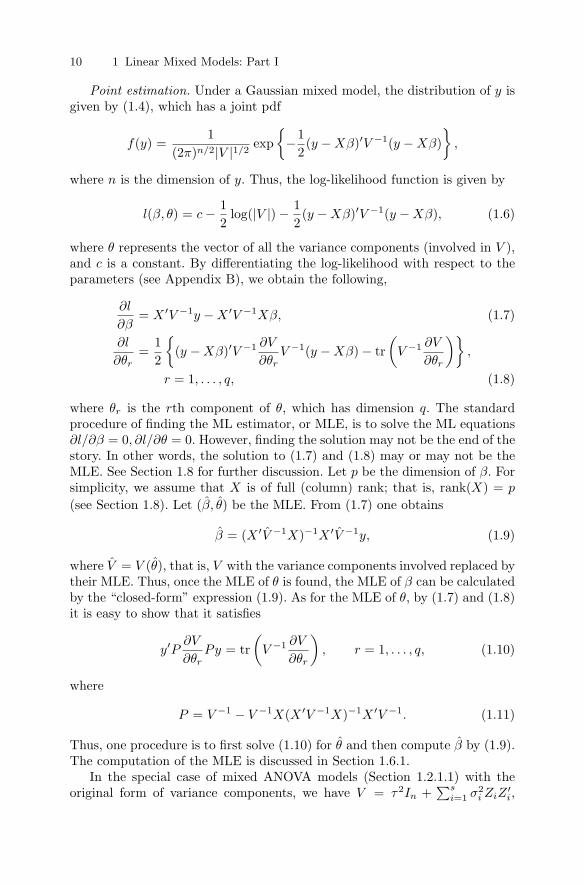
Point estimation. Under a Gaussian mixed model, the distribution of y isgiven by (1.4), which has a joint pdf

f(y) =1

(2π)n/2|V |1/2 exp{

−12(y − Xβ)′V −1(y − Xβ)

},

where n is the dimension of y. Thus, the log-likelihood function is given by

l(β, θ) = c − 12

log(|V |) − 12(y − Xβ)′V −1(y − Xβ), (1.6)

where θ represents the vector of all the variance components (involved in V ),and c is a constant. By differentiating the log-likelihood with respect to theparameters (see Appendix B), we obtain the following,

∂l

∂β= X ′V −1y − X ′V −1Xβ, (1.7)

∂l

∂θr=

12

{(y − Xβ)′V −1 ∂V

∂θrV −1(y − Xβ) − tr

(V −1 ∂V

∂θr

)},

r = 1, . . . , q, (1.8)

where θr is the rth component of θ, which has dimension q. The standardprocedure of finding the ML estimator, or MLE, is to solve the ML equations∂l/∂β = 0, ∂l/∂θ = 0. However, finding the solution may not be the end of thestory. In other words, the solution to (1.7) and (1.8) may or may not be theMLE. See Section 1.8 for further discussion. Let p be the dimension of β. Forsimplicity, we assume that X is of full (column) rank; that is, rank(X) = p

(see Section 1.8). Let (β, θ) be the MLE. From (1.7) one obtains

β = (X ′V −1X)−1X ′V −1y, (1.9)

where V = V (θ), that is, V with the variance components involved replaced bytheir MLE. Thus, once the MLE of θ is found, the MLE of β can be calculatedby the “closed-form” expression (1.9). As for the MLE of θ, by (1.7) and (1.8)it is easy to show that it satisfies

y′P∂V

∂θrPy = tr

(V −1 ∂V

∂θr

), r = 1, . . . , q, (1.10)

where

P = V −1 − V −1X(X ′V −1X)−1X ′V −1. (1.11)

Thus, one procedure is to first solve (1.10) for θ and then compute β by (1.9).The computation of the MLE is discussed in Section 1.6.1.

In the special case of mixed ANOVA models (Section 1.2.1.1) with theoriginal form of variance components, we have V = τ2In +

∑si=1 σ2

i ZiZ′i,


hence ∂V/∂τ2 = In, ∂V/∂σ2i = ZiZ

′i, 1 ≤ i ≤ s. Similarly, with the Hartley–

Rao form, we have V = λ(In +∑s

i=1 γiZiZ′i), hence ∂V/∂λ = V/λ, ∂V/∂γi =

λZiZ′i, 1 ≤ i ≤ s. With these expressions, the above equations may be further

simplified. As for the longitudinal model (Section 1.2.1.2), the specification of(1.7)–(1.10) is left as an exercise (see Exercise 1.5).

For mixed ANOVA models (Section 1.2.1.1), asymptotic properties of theMLE, including consistency and asymptotic normality, were first studied byHartley and Rao (1967). Also see Anderson (1969, 1971a), who studied asymp-totic properties of the MLE under the marginal model (Section 1.2.1.3) with alinear covariance structure; and Miller (1977). In these papers the authors haveassumed that the number of fixed effects (i.e., p) remains fixed or bounded asthe sample size n increases. As it turns out, this assumption is critical to en-sure consistency of the MLE. See Example 1.7 below. Jiang (1996) consideredasymptotic behavior of the MLE when p increases with n, and compared itwith that of the REML estimator. The results hold for non-Gaussian mixedANOVA models (Section 1.2.2.1), which include the Gaussian case. See Sec-tion 1.8 for more details.

Asymptotic covariance matrix. Under suitable conditions (see Section 1.8for discussion), the MLE is consistent and asymptotically normal with theasymptotic covariance matrix equal to the inverse of the Fisher informationmatrix. Let ψ = (β′, θ′)′. Then, under regularity conditions, the Fisher infor-mation matrix has the following expressions,

Var(

∂l

∂ψ

)= −E

(∂2l

∂ψ∂ψ′

). (1.12)

By (1.7) and (1.8), further expressions can be obtained for the elements of(1.12). For example, assuming that V is twice continuously differentiable (withrespect to the components of θ), then, using the results of Appendices B andC, it can be shown (Exercise 1.6) that

E(

∂2l

∂β∂β′

)= −X ′V −1X, (1.13)

E(

∂2l

∂β∂θr

)= 0, 1 ≤ r ≤ q, (1.14)

E(

∂2l

∂θr∂θs

)= −1

2tr(

V −1 ∂V

∂θrV −1 ∂V

∂θs

), 1 ≤ r, s ≤ q. (1.15)

It follows that (1.12) does not depend on β, and therefore may be denoted byI(θ), as we do in the sequel.

We now consider some examples.

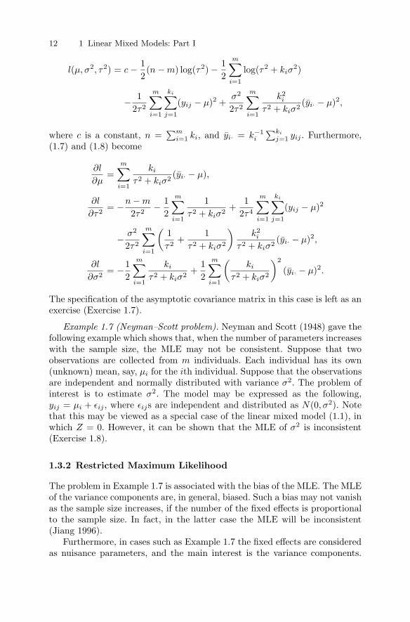
Example 1.1 (Continued). It can be shown (see Exercise 1.7) that, in thiscase, (1.6) has the following expression,


l(µ, σ2, τ2) = c − 12(n − m) log(τ2) − 1

2

m∑i=1

log(τ2 + kiσ2)

− 12τ2

m∑i=1

ki∑j=1

(yij − µ)2 +σ2

2τ2

m∑i=1

k2i

τ2 + kiσ2 (yi· − µ)2,

where c is a constant, n =∑m

i=1 ki, and yi· = k−1i

∑ki

j=1 yij . Furthermore,(1.7) and (1.8) become

∂l

∂µ=

m∑i=1

ki

τ2 + kiσ2 (yi· − µ),

∂l

∂τ2 = −n − m

2τ2 − 12

m∑i=1

1τ2 + kiσ2 +

12τ4

m∑i=1

ki∑j=1

(yij − µ)2

− σ2

2τ2

m∑i=1

(1τ2 +

1τ2 + kiσ2

)k2

i

τ2 + kiσ2 (yi· − µ)2,

∂l

∂σ2 = −12

m∑i=1

ki

τ2 + kiσ2 +12

m∑i=1

(ki

τ2 + kiσ2

)2

(yi· − µ)2.

The specification of the asymptotic covariance matrix in this case is left as anexercise (Exercise 1.7).

Example 1.7 (Neyman–Scott problem). Neyman and Scott (1948) gave thefollowing example which shows that, when the number of parameters increaseswith the sample size, the MLE may not be consistent. Suppose that twoobservations are collected from m individuals. Each individual has its own(unknown) mean, say, µi for the ith individual. Suppose that the observationsare independent and normally distributed with variance σ2. The problem ofinterest is to estimate σ2. The model may be expressed as the following,yij = µi + εij , where εijs are independent and distributed as N(0, σ2). Notethat this may be viewed as a special case of the linear mixed model (1.1), inwhich Z = 0. However, it can be shown that the MLE of σ2 is inconsistent(Exercise 1.8).

1.3.2 Restricted Maximum Likelihood

The problem in Example 1.7 is associated with the bias of the MLE. The MLEof the variance components are, in general, biased. Such a bias may not vanishas the sample size increases, if the number of the fixed effects is proportionalto the sample size. In fact, in the latter case the MLE will be inconsistent(Jiang 1996).

Furthermore, in cases such as Example 1.7 the fixed effects are consideredas nuisance parameters, and the main interest is the variance components.


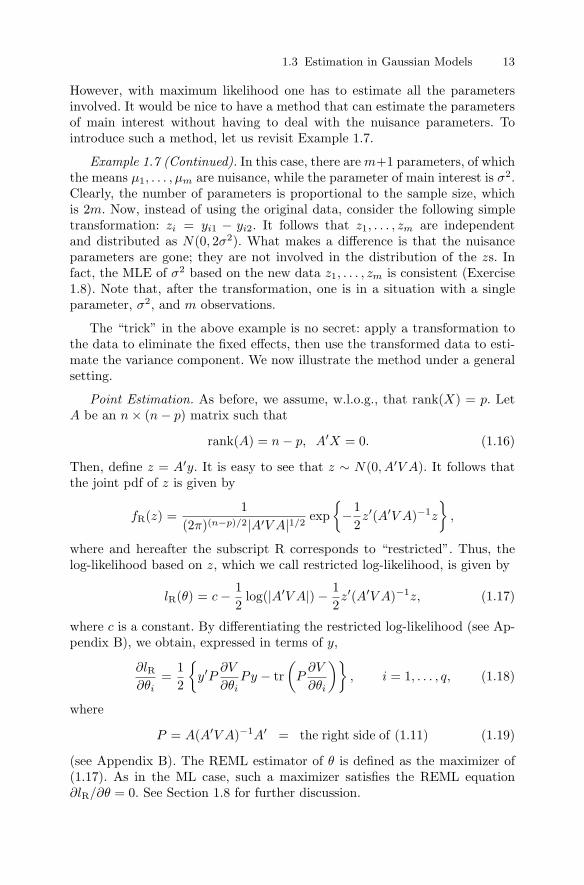
However, with maximum likelihood one has to estimate all the parametersinvolved. It would be nice to have a method that can estimate the parametersof main interest without having to deal with the nuisance parameters. Tointroduce such a method, let us revisit Example 1.7.

Example 1.7 (Continued). In this case, there are m+1 parameters, of whichthe means µ1, . . . , µm are nuisance, while the parameter of main interest is σ2.Clearly, the number of parameters is proportional to the sample size, whichis 2m. Now, instead of using the original data, consider the following simpletransformation: zi = yi1 − yi2. It follows that z1, . . . , zm are independentand distributed as N(0, 2σ2). What makes a difference is that the nuisanceparameters are gone; they are not involved in the distribution of the zs. Infact, the MLE of σ2 based on the new data z1, . . . , zm is consistent (Exercise1.8). Note that, after the transformation, one is in a situation with a singleparameter, σ2, and m observations.

The “trick” in the above example is no secret: apply a transformation tothe data to eliminate the fixed effects, then use the transformed data to esti-mate the variance component. We now illustrate the method under a generalsetting.

Point Estimation. As before, we assume, w.l.o.g., that rank(X) = p. LetA be an n × (n − p) matrix such that

rank(A) = n − p, A′X = 0. (1.16)

Then, define z = A′y. It is easy to see that z ∼ N(0, A′V A). It follows thatthe joint pdf of z is given by

fR(z) =1

(2π)(n−p)/2|A′V A|1/2 exp{

−12z′(A′V A)−1z

},

where and hereafter the subscript R corresponds to “restricted”. Thus, thelog-likelihood based on z, which we call restricted log-likelihood, is given by

lR(θ) = c − 12

log(|A′V A|) − 12z′(A′V A)−1z, (1.17)

where c is a constant. By differentiating the restricted log-likelihood (see Ap-pendix B), we obtain, expressed in terms of y,

∂lR∂θi

=12

{y′P

∂V

∂θiPy − tr

(P

∂V

∂θi

)}, i = 1, . . . , q, (1.18)

where

P = A(A′V A)−1A′ = the right side of (1.11) (1.19)

(see Appendix B). The REML estimator of θ is defined as the maximizer of(1.17). As in the ML case, such a maximizer satisfies the REML equation∂lR/∂θ = 0. See Section 1.8 for further discussion.


Remark. Although the REML estimator is defined through a transformingmatrix A, the REML estimator, in fact, does not depend on A. To see this,note that, by (1.18) and (1.19), the REML equations do not depend on A. Amore thorough demonstration is left as an exercise (Exercise 1.9). This factis important because, obviously, the choice of A is not unique, and one doesnot want the estimator to depend on the choice of the transformation.

Example 1.7 (Continued). It is easy to see that the transformation zi =yi1 − yi2, i = 1, . . . , m corresponds to

A =

⎛⎜⎜⎜⎝1 −1 0 0 · · · 0 00 0 1 −1 · · · 0 0...

......

......

......

0 0 0 0 · · · 1 −1

⎞⎟⎟⎟⎠′

.

An alternative transforming matrix may be obtained as B = AT , where T isany m × m nonsingular matrix. But the resulting REML estimator of σ2 isthe same (Exercise 1.9).

Historical note. The REML method was first proposed by Thompson(1962) and was put on a broad basis by Patterson and Thompson (1971).The method is also known as residual maximum likelihood, although the ab-breviation, REML, remains the same. There have been different derivations ofREML. For example, Harville (1974) provided a Bayesian derivation of REML.He showed that the restricted likelihood can be derived as the marginal likeli-hood when β is integrated out under a noninformative, or flat, prior (Exercise1.10). Also see Verbyla (1990). Barndorff-Nielsen (1983) derived the restrictedlikelihood as a modified profile likelihood. More recently, Jiang (1996) pointedout that the REML equations may be derived under the assumption of a mul-tivariate t-distribution (instead of multivariate normal distribution). Moregenerally, Heyde (1994) showed that the REML equations may be viewed asquasi-likelihood equations. See Heyde (1997) for further details. Surveys onREML can be found in Harville (1977), Khuri and Sahai (1985), Robinson(1987), and Speed (1997).

Note that the restricted log-likelihood (1.17) is a function of θ only. In otherwords, the REML method is a method of estimating θ (not β, because thelatter is eliminated before the estimation). However, once the REML estimatorof θ is obtained, β is usually estimated the same way as the ML, that is, by(1.9), where V = V (θ) with θ being the REML estimator. Such an estimatoris sometimes referred as the “REML estimator” of β.

Asymptotic covariance matrix. Under suitable conditions, the REML esti-mator is consistent and asymptotically normal (see Section 1.8 for discussion).The asymptotic covariance matrix is equal to the inverse of the restrictedFisher information matrix, which, under regularity conditions, has similar ex-pressions as (1.12):

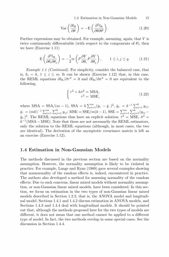
1.4 Estimation in Non-Gaussian Models 15

Var(

∂lR∂θ

)= −E

(∂2lR∂θ∂θ′

). (1.20)

Further expressions may be obtained. For example, assuming, again, that V istwice continuously differentiable (with respect to the components of θ), thenwe have (Exercise 1.11)

E(

∂2lR∂θi∂θj

)= −1

2tr(

P∂V

∂θiP

∂V

∂θj

), 1 ≤ i, j ≤ q. (1.21)

Example 1.1 (Continued). For simplicity, consider the balanced case, thatis, ki = k, 1 ≤ i ≤ m. It can be shown (Exercise 1.12) that, in this case,the REML equations ∂lR/∂τ2 = 0 and ∂lR/∂σ2 = 0 are equivalent to thefollowing, {

τ2 + kσ2 = MSA,τ2 = MSE,

(1.22)

where MSA = SSA/(m − 1), SSA = k∑m

i=1(yi· − y··)2, yi· = k−1 ∑kj=1 yij ,

y·· = (mk)−1 ∑mi=1

∑kj=1 yij ; MSE = SSE/m(k −1), SSE =

∑mi=1

∑kj=1(yij −

yi·)2. The REML equations thus have an explicit solution: τ2 = MSE, σ2 =k−1(MSA−MSE). Note that these are not necessarily the REML estimators,only the solution to the REML equations (although, in most cases, the twoare identical). The derivation of the asymptotic covariance matrix is left asan exercise (Exercise 1.12).

1.4 Estimation in Non-Gaussian Models

The methods discussed in the previous section are based on the normalityassumption. However, the normality assumption is likely to be violated inpractice. For example, Lange and Ryan (1989) gave several examples showingthat nonnormality of the random effects is, indeed, encountered in practice.The authors also developed a method for assessing normality of the randomeffects. Due to such concerns, linear mixed models without normality assump-tion, or non-Gaussian linear mixed models, have been considered. In this sec-tion, we focus on estimation in the two types of non-Gaussian linear mixedmodels described in Section 1.2.2, that is, the ANOVA model and longitudi-nal model. Sections 1.4.1 and 1.4.2 discuss estimation in ANOVA models, andSections 1.4.3 and 1.4.4 deal with longitudinal models. It should be pointedout that, although the methods proposed here for the two types of models aredifferent, it does not mean that one method cannot be applied to a differenttype of model. In fact, the two methods overlap in some special cases. See thediscussion in Section 1.4.4.

springer series in statistics - download.e-bookshelf.de · brockwell/davis: time series: theory and...

Documents