spss neural networks™ 17 - salem state universityw3.salemstate.edu/~gsmith/help/files/spss17/spss...
TRANSCRIPT

i
SPSS Neural Networks™ 17.0

For more information about SPSS Inc. software products, please visit our Web site at http://www.spss.com or contact
SPSS Inc.233 South Wacker Drive, 11th FloorChicago, IL 60606-6412Tel: (312) 651-3000Fax: (312) 651-3668
SPSS is a registered trademark and the other product names are the trademarks of SPSS Inc. for its proprietary computersoftware. No material describing such software may be produced or distributed without the written permission of theowners of the trademark and license rights in the software and the copyrights in the published materials.
The SOFTWARE and documentation are provided with RESTRICTED RIGHTS. Use, duplication, or disclosure bythe Government is subject to restrictions as set forth in subdivision (c) (1) (ii) of The Rights in Technical Data andComputer Software clause at 52.227-7013. Contractor/manufacturer is SPSS Inc., 233 South Wacker Drive, 11thFloor, Chicago, IL 60606-6412.Patent No. 7,023,453
General notice: Other product names mentioned herein are used for identification purposes only and may be trademarksof their respective companies.
Windows is a registered trademark of Microsoft Corporation.
Apple, Mac, and the Mac logo are trademarks of Apple Computer, Inc., registered in the U.S. and other countries.
This product uses WinWrap Basic, Copyright 1993-2007, Polar Engineering and Consulting, http://www.winwrap.com.
Printed in the United States of America.
No part of this publication may be reproduced, stored in a retrieval system, or transmitted, in any form or by any means,electronic, mechanical, photocopying, recording, or otherwise, without the prior written permission of the publisher.

Preface
SPSS Statistics 17.0 is a comprehensive system for analyzing data. The NeuralNetworks optional add-on module provides the additional analytic techniquesdescribed in this manual. The Neural Networks add-on module must be used with theSPSS Statistics 17.0 Base system and is completely integrated into that system.
Installation
To install the Neural Networks add-on module, run the License Authorization Wizardusing the authorization code that you received from SPSS Inc. For more information,see the installation instructions supplied with the Neural Networks add-on module.
Compatibility
SPSS Statistics is designed to run on many computer systems. See the installationinstructions that came with your system for specific information on minimum andrecommended requirements.
Serial Numbers
Your serial number is your identification number with SPSS Inc. You will need thisserial number when you contact SPSS Inc. for information regarding support, payment,or an upgraded system. The serial number was provided with your Base system.
Customer Service
If you have any questions concerning your shipment or account, contact your localoffice, listed on the Web site at http://www.spss.com/worldwide. Please have yourserial number ready for identification.
iii

Training Seminars
SPSS Inc. provides both public and onsite training seminars. All seminars featurehands-on workshops. Seminars will be offered in major cities on a regular basis.For more information on these seminars, contact your local office, listed on the Website at http://www.spss.com/worldwide.
Technical Support
Technical Support services are available to maintenance customers. Customers maycontact Technical Support for assistance in using SPSS Statistics or for installationhelp for one of the supported hardware environments. To reach Technical Support,see the Web site at http://www.spss.com, or contact your local office, listed on theWeb site at http://www.spss.com/worldwide. Be prepared to identify yourself, yourorganization, and the serial number of your system.
Additional PublicationsThe SPSS Statistical Procedures Companion, by Marija Norušis, has been published
by Prentice Hall. A new version of this book, updated for SPSS Statistics 17.0,is planned. The SPSS Advanced Statistical Procedures Companion, also basedon SPSS Statistics 17.0, is forthcoming. The SPSS Guide to Data Analysis forSPSS Statistics 17.0 is also in development. Announcements of publicationsavailable exclusively through Prentice Hall will be available on the Web site athttp://www.spss.com/estore (select your home country, and then click Books).
iv
Contents
Part I: User's Guide
1 Introduction to Neural Networks 1
What Is a Neural Network?. . . . . . . . . . . . . . . . . . . . . . . . . . . . . . . . . . . . . . . 1Neural Network Structure . . . . . . . . . . . . . . . . . . . . . . . . . . . . . . . . . . . . . . . 3
2 Multilayer Perceptron 5
Partitions . . . . . . . . . . . . . . . . . . . . . . . . . . . . . . . . . . . . . . . . . . . . . . . . . . . 11Architecture . . . . . . . . . . . . . . . . . . . . . . . . . . . . . . . . . . . . . . . . . . . . . . . . 13Training . . . . . . . . . . . . . . . . . . . . . . . . . . . . . . . . . . . . . . . . . . . . . . . . . . . . 16Output . . . . . . . . . . . . . . . . . . . . . . . . . . . . . . . . . . . . . . . . . . . . . . . . . . . . . 19Save . . . . . . . . . . . . . . . . . . . . . . . . . . . . . . . . . . . . . . . . . . . . . . . . . . . . . . 22Export . . . . . . . . . . . . . . . . . . . . . . . . . . . . . . . . . . . . . . . . . . . . . . . . . . . . . 24Options . . . . . . . . . . . . . . . . . . . . . . . . . . . . . . . . . . . . . . . . . . . . . . . . . . . . 25
3 Radial Basis Function 28
Partitions . . . . . . . . . . . . . . . . . . . . . . . . . . . . . . . . . . . . . . . . . . . . . . . . . . . 33Architecture . . . . . . . . . . . . . . . . . . . . . . . . . . . . . . . . . . . . . . . . . . . . . . . . 35Output . . . . . . . . . . . . . . . . . . . . . . . . . . . . . . . . . . . . . . . . . . . . . . . . . . . . . 37Save . . . . . . . . . . . . . . . . . . . . . . . . . . . . . . . . . . . . . . . . . . . . . . . . . . . . . . 40Export . . . . . . . . . . . . . . . . . . . . . . . . . . . . . . . . . . . . . . . . . . . . . . . . . . . . . 42Options . . . . . . . . . . . . . . . . . . . . . . . . . . . . . . . . . . . . . . . . . . . . . . . . . . . . 43
v
Part II: Examples
4 Multilayer Perceptron 45
Using a Multilayer Perceptron to Assess Credit Risk . . . . . . . . . . . . . . . . . . . 45Preparing the Data for Analysis . . . . . . . . . . . . . . . . . . . . . . . . . . . . . . . 45Running the Analysis . . . . . . . . . . . . . . . . . . . . . . . . . . . . . . . . . . . . . . . 48Case Processing Summary . . . . . . . . . . . . . . . . . . . . . . . . . . . . . . . . . . 52Network Information . . . . . . . . . . . . . . . . . . . . . . . . . . . . . . . . . . . . . . . 52Model Summary . . . . . . . . . . . . . . . . . . . . . . . . . . . . . . . . . . . . . . . . . . 53Classification. . . . . . . . . . . . . . . . . . . . . . . . . . . . . . . . . . . . . . . . . . . . . 54Correcting Overtraining . . . . . . . . . . . . . . . . . . . . . . . . . . . . . . . . . . . . . 54Summary . . . . . . . . . . . . . . . . . . . . . . . . . . . . . . . . . . . . . . . . . . . . . . . . 69
Using a Multilayer Perceptron to Estimate Healthcare Costs and Lengths ofStay . . . . . . . . . . . . . . . . . . . . . . . . . . . . . . . . . . . . . . . . . . . . . . . . . . . . . . . 70
Preparing the Data for Analysis . . . . . . . . . . . . . . . . . . . . . . . . . . . . . . . 70Running the Analysis . . . . . . . . . . . . . . . . . . . . . . . . . . . . . . . . . . . . . . . 71Warnings. . . . . . . . . . . . . . . . . . . . . . . . . . . . . . . . . . . . . . . . . . . . . . . . 80Case Processing Summary . . . . . . . . . . . . . . . . . . . . . . . . . . . . . . . . . . 80Network Information . . . . . . . . . . . . . . . . . . . . . . . . . . . . . . . . . . . . . . . 81Model Summary . . . . . . . . . . . . . . . . . . . . . . . . . . . . . . . . . . . . . . . . . . 82Predicted-by-Observed Charts. . . . . . . . . . . . . . . . . . . . . . . . . . . . . . . . 84Residual-by-Predicted Charts . . . . . . . . . . . . . . . . . . . . . . . . . . . . . . . . 86Independent Variable Importance . . . . . . . . . . . . . . . . . . . . . . . . . . . . . 88Summary . . . . . . . . . . . . . . . . . . . . . . . . . . . . . . . . . . . . . . . . . . . . . . . . 88
Recommended Readings . . . . . . . . . . . . . . . . . . . . . . . . . . . . . . . . . . . . . . . 89
5 Radial Basis Function 90
Using Radial Basis Function to Classify Telecommunications Customers . . . . 90Preparing the Data for Analysis . . . . . . . . . . . . . . . . . . . . . . . . . . . . . . . 90
vi
Running the Analysis . . . . . . . . . . . . . . . . . . . . . . . . . . . . . . . . . . . . . . . 91Case Processing Summary . . . . . . . . . . . . . . . . . . . . . . . . . . . . . . . . . . 97Network Information . . . . . . . . . . . . . . . . . . . . . . . . . . . . . . . . . . . . . . . 98Model Summary . . . . . . . . . . . . . . . . . . . . . . . . . . . . . . . . . . . . . . . . . . 99Classification. . . . . . . . . . . . . . . . . . . . . . . . . . . . . . . . . . . . . . . . . . . . 100Predicted-by-Observed Chart . . . . . . . . . . . . . . . . . . . . . . . . . . . . . . . 101ROC Curve . . . . . . . . . . . . . . . . . . . . . . . . . . . . . . . . . . . . . . . . . . . . . . 103Cumulative Gains and Lift Charts . . . . . . . . . . . . . . . . . . . . . . . . . . . . . 105
Recommended Readings . . . . . . . . . . . . . . . . . . . . . . . . . . . . . . . . . . . . . . 107
Appendix
A Sample Files 108
Bibliography 122
Index 124
vii


Part I:User's Guide


Chapter
1Introduction to Neural Networks
Neural networks are the preferred tool for many predictive data mining applicationsbecause of their power, flexibility, and ease of use. Predictive neural networks areparticularly useful in applications where the underlying process is complex, such as:
Forecasting consumer demand to streamline production and delivery costs.Predicting the probability of response to direct mail marketing to determine whichhouseholds on a mailing list should be sent an offer.Scoring an applicant to determine the risk of extending credit to the applicant.Detecting fraudulent transactions in an insurance claims database.
Neural networks used in predictive applications, such as the multilayer perceptron(MLP) and radial basis function (RBF) networks, are supervised in the sense that themodel-predicted results can be compared against known values of the target variables.The Neural Networks option allows you to fit MLP and RBF networks and save theresulting models for scoring.
What Is a Neural Network?
The term neural network applies to a loosely related family of models, characterizedby a large parameter space and flexible structure, descending from studies ofbrain functioning. As the family grew, most of the new models were designed fornonbiological applications, though much of the associated terminology reflects itsorigin.
1
2
Chapter 1
Specific definitions of neural networks are as varied as the fields in which they areused. While no single definition properly covers the entire family of models, for now,consider the following description (Haykin, 1998):
A neural network is a massively parallel distributed processor that has a naturalpropensity for storing experiential knowledge and making it available for use. Itresembles the brain in two respects:
Knowledge is acquired by the network through a learning process.Interneuron connection strengths known as synaptic weights are used to storethe knowledge.
For a discussion of why this definition is perhaps too restrictive, see (Ripley, 1996).
In order to differentiate neural networks from traditional statistical methods using thisdefinition, what is not said is just as significant as the actual text of the definition. Forexample, the traditional linear regression model can acquire knowledge through theleast-squares method and store that knowledge in the regression coefficients. In thissense, it is a neural network. In fact, you can argue that linear regression is a specialcase of certain neural networks. However, linear regression has a rigid model structureand set of assumptions that are imposed before learning from the data.By contrast, the definition above makes minimal demands on model structure and
assumptions. Thus, a neural network can approximate a wide range of statisticalmodels without requiring that you hypothesize in advance certain relationships betweenthe dependent and independent variables. Instead, the form of the relationships isdetermined during the learning process. If a linear relationship between the dependentand independent variables is appropriate, the results of the neural network shouldclosely approximate those of the linear regression model. If a nonlinear relationshipis more appropriate, the neural network will automatically approximate the “correct”model structure.The trade-off for this flexibility is that the synaptic weights of a neural network are
not easily interpretable. Thus, if you are trying to explain an underlying process thatproduces the relationships between the dependent and independent variables, it wouldbe better to use a more traditional statistical model. However, if model interpretabilityis not important, you can often obtain good model results more quickly using a neuralnetwork.
3
Introduction to Neural Networks
Neural Network Structure
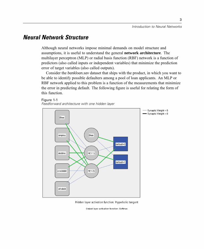
Although neural networks impose minimal demands on model structure andassumptions, it is useful to understand the general network architecture. Themultilayer perceptron (MLP) or radial basis function (RBF) network is a function ofpredictors (also called inputs or independent variables) that minimize the predictionerror of target variables (also called outputs).Consider the bankloan.sav dataset that ships with the product, in which you want to
be able to identify possible defaulters among a pool of loan applicants. An MLP orRBF network applied to this problem is a function of the measurements that minimizethe error in predicting default. The following figure is useful for relating the form ofthis function.
Figure 1-1Feedforward architecture with one hidden layer

4
Chapter 1
This structure is known as a feedforward architecture because the connections in thenetwork flow forward from the input layer to the output layer without any feedbackloops. In this figure:
The input layer contains the predictors.The hidden layer contains unobservable nodes, or units. The value of each hiddenunit is some function of the predictors; the exact form of the function depends inpart upon the network type and in part upon user-controllable specifications.The output layer contains the responses. Since the history of default is acategorical variable with two categories, it is recoded as two indicator variables.Each output unit is some function of the hidden units. Again, the exact form ofthe function depends in part on the network type and in part on user-controllablespecifications.
The MLP network allows a second hidden layer; in that case, each unit of the secondhidden layer is a function of the units in the first hidden layer, and each response is afunction of the units in the second hidden layer.
Chapter
2Multilayer Perceptron
The Multilayer Perceptron (MLP) procedure produces a predictive model for one ormore dependent (target) variables based on the values of the predictor variables.
Examples. Following are two scenarios using the MLP procedure:
A loan officer at a bank needs to be able to identify characteristics that are indicativeof people who are likely to default on loans and use those characteristics to identifygood and bad credit risks. Using a sample of past customers, she can train a multilayerperceptron, validate the analysis using a holdout sample of past customers, and thenuse the network to classify prospective customers as good or bad credit risks.
A hospital system is interested in tracking costs and lengths of stay for patientsadmitted for treatment of myocardial infarction (MI, or “heart attack”). Obtainingaccurate estimates of these measures allows the administration to properly manage theavailable bed space as patients are treated. Using the treatment records of a sampleof patients who received treatment for MI, the administrator can train a network topredict both cost and length of stay.
Dependent variables. The dependent variables can be:Nominal. A variable can be treated as nominal when its values represent categorieswith no intrinsic ranking (for example, the department of the company in whichan employee works). Examples of nominal variables include region, zip code,and religious affiliation.Ordinal. A variable can be treated as ordinal when its values represent categorieswith some intrinsic ranking (for example, levels of service satisfaction fromhighly dissatisfied to highly satisfied). Examples of ordinal variables include
5
6
Chapter 2
attitude scores representing degree of satisfaction or confidence and preferencerating scores.Scale. A variable can be treated as scale when its values represent orderedcategories with a meaningful metric, so that distance comparisons between valuesare appropriate. Examples of scale variables include age in years and incomein thousands of dollars.The procedure assumes that the appropriate measurement level has been assignedto all dependent variables; however, you can temporarily change the measurementlevel for a variable by right-clicking the variable in the source variable list andselecting a measurement level from the context menu.
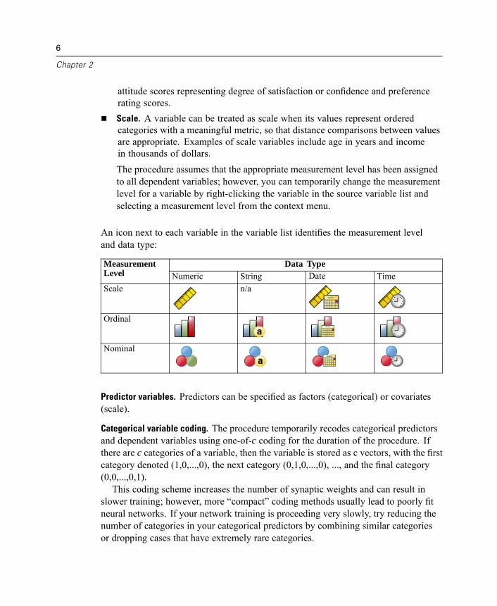
An icon next to each variable in the variable list identifies the measurement leveland data type:
Data TypeMeasurementLevel Numeric String Date TimeScale n/a
Ordinal
Nominal
Predictor variables. Predictors can be specified as factors (categorical) or covariates(scale).
Categorical variable coding. The procedure temporarily recodes categorical predictorsand dependent variables using one-of-c coding for the duration of the procedure. Ifthere are c categories of a variable, then the variable is stored as c vectors, with the firstcategory denoted (1,0,...,0), the next category (0,1,0,...,0), ..., and the final category(0,0,...,0,1).This coding scheme increases the number of synaptic weights and can result in
slower training; however, more “compact” coding methods usually lead to poorly fitneural networks. If your network training is proceeding very slowly, try reducing thenumber of categories in your categorical predictors by combining similar categoriesor dropping cases that have extremely rare categories.

7
Multilayer Perceptron
All one-of-c coding is based on the training data, even if a testing or holdout sampleis defined (see Partitions on p. 11). Thus, if the testing or holdout samples containcases with predictor categories that are not present in the training data, then those casesare not used by the procedure or in scoring. If the testing or holdout samples containcases with dependent variable categories that are not present in the training data, thenthose cases are not used by the procedure, but they may be scored.
Rescaling. Scale-dependent variables and covariates are rescaled by default to improvenetwork training. All rescaling is performed based on the training data, even if atesting or holdout sample is defined (see Partitions on p. 11). That is, depending on thetype of rescaling, the mean, standard deviation, minimum value, or maximum valueof a covariate or dependent variable is computed using only the training data. If youspecify a variable to define partitions, it is important that these covariates or dependentvariables have similar distributions across the training, testing, and holdout samples.
Frequency weights. Frequency weights are ignored by this procedure.
Replicating results. If you want to replicate your results exactly, use the sameinitialization value for the random number generator, the same data order, and thesame variable order, in addition to using the same procedure settings. More details onthis issue follow:
Random number generation. The procedure uses random number generationduring random assignment of partitions, random subsampling for initialization ofsynaptic weights, random subsampling for automatic architecture selection, andthe simulated annealing algorithm used in weight initialization and automaticarchitecture selection. To reproduce the same randomized results in the future,use the same initialization value for the random number generator before eachrun of the Multilayer Perceptron procedure. See Preparing the Data for Analysison p. 45 for step-by-step instructions.Case order. The Online and Mini-batch training methods (see Training on p.16) are explicitly dependent upon case order; however, even Batch training isdependent upon case order because initialization of synaptic weights involvessubsampling from the dataset.

8
Chapter 2
To minimize order effects, randomly order the cases. To verify the stability of agiven solution, you may want to obtain several different solutions with cases sortedin different random orders. In situations with extremely large file sizes, multipleruns can be performed with a sample of cases sorted in different random orders.Variable order. Results may be influenced by the order of variables in the factorand covariate lists due to the different pattern of initial values assigned when thevariable order is changed. As with case order effects, you might try differentvariable orders (simply drag and drop within the factor and covariate lists) toassess the stability of a given solution.
Creating a Multilayer Perceptron Network
From the menus choose:Analyze
Neural NetworksMultilayer Perceptron...
9
Multilayer Perceptron
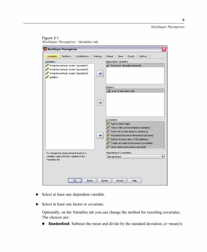
Figure 2-1Multilayer Perceptron: Variables tab
E Select at least one dependent variable.
E Select at least one factor or covariate.
Optionally, on the Variables tab you can change the method for rescaling covariates.The choices are:
Standardized. Subtract the mean and divide by the standard deviation, (x−mean)/s.

10
Chapter 2
Normalized. Subtract the minimum and divide by the range, (x−min)/(max−min).Normalized values fall between 0 and 1.Adjusted Normalized. Adjusted version of subtracting the minimum and dividingby the range, [2*(x−min)/(max−min)]−1. Adjusted normalized values fall between−1 and 1.None. No rescaling of covariates.
11
Multilayer Perceptron
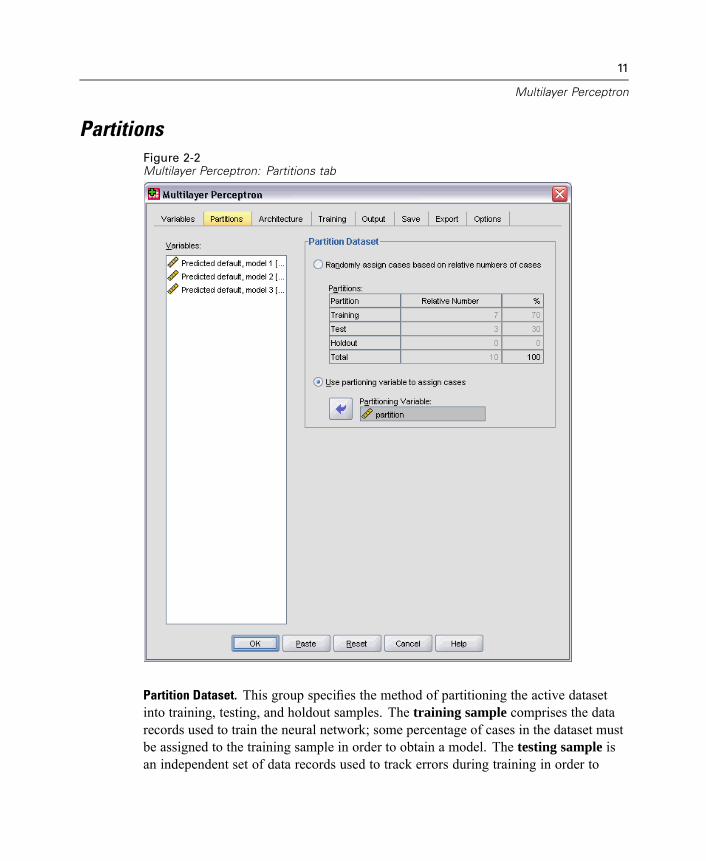
PartitionsFigure 2-2Multilayer Perceptron: Partitions tab
Partition Dataset. This group specifies the method of partitioning the active datasetinto training, testing, and holdout samples. The training sample comprises the datarecords used to train the neural network; some percentage of cases in the dataset mustbe assigned to the training sample in order to obtain a model. The testing sample isan independent set of data records used to track errors during training in order to
12
Chapter 2
prevent overtraining. It is highly recommended that you create a training sample,and network training will generally be most efficient if the testing sample is smallerthan the training sample. The holdout sample is another independent set of datarecords used to assess the final neural network; the error for the holdout sample givesan “honest” estimate of the predictive ability of the model because the holdout caseswere not used to build the model.
Randomly assign cases based on relative number of cases. Specify the relativenumber (ratio) of cases randomly assigned to each sample (training, testing, andholdout). The % column reports the percentage of cases that will be assigned toeach sample based on the relative numbers you have specified.For example, specifying 7, 3, 0 as the relative numbers for training, testing, andholdout samples corresponds to 70%, 30%, and 0%. Specifying 2, 1, 1 as therelative numbers corresponds to 50%, 25%, and 25%; 1, 1, 1 corresponds todividing the dataset into equal thirds among training, testing, and holdout.Use partitioning variable to assign cases. Specify a numeric variable that assignseach case in the active dataset to the training, testing, or holdout sample. Caseswith a positive value on the variable are assigned to the training sample, cases witha value of 0, to the testing sample, and cases with a negative value, to the holdoutsample. Cases with a system-missing value are excluded from the analysis. Anyuser-missing values for the partition variable are always treated as valid.Note: Using a partitioning variable will not guarantee identical results insuccessive runs of the procedure. See “Replicating results” in the main MultilayerPerceptron topic.
13
Multilayer Perceptron
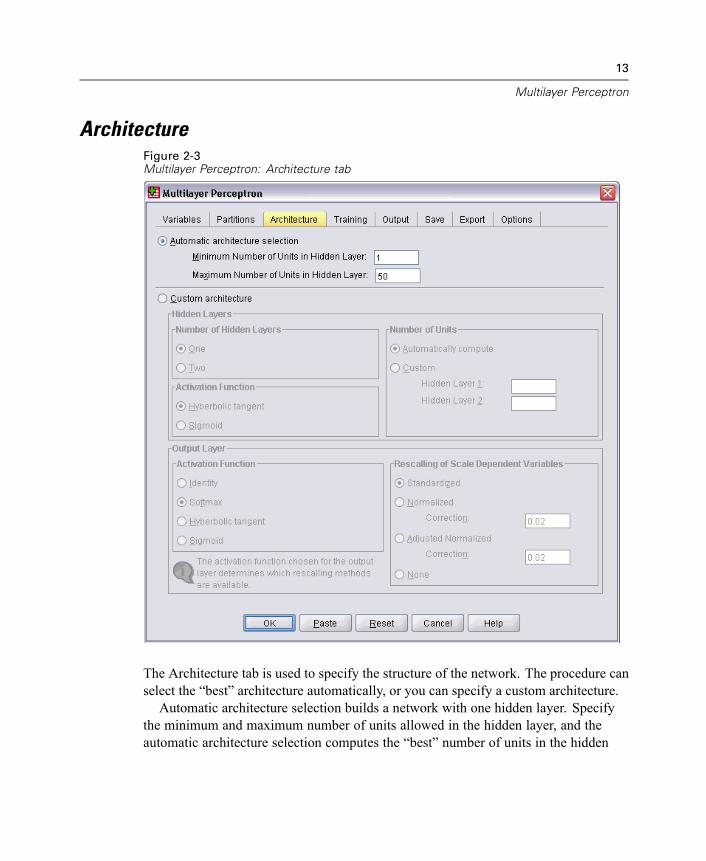
ArchitectureFigure 2-3Multilayer Perceptron: Architecture tab
The Architecture tab is used to specify the structure of the network. The procedure canselect the “best” architecture automatically, or you can specify a custom architecture.Automatic architecture selection builds a network with one hidden layer. Specify
the minimum and maximum number of units allowed in the hidden layer, and theautomatic architecture selection computes the “best” number of units in the hidden
14
Chapter 2
layer. Automatic architecture selection uses the default activation functions for thehidden and output layers.Custom architecture selection gives you expert control over the hidden and output
layers and can be most useful when you know in advance what architecture you wantor when you need to tweak the results of the Automatic architecture selection.
Hidden Layers
The hidden layer contains unobservable network nodes (units). Each hidden unit is afunction of the weighted sum of the inputs. The function is the activation function, andthe values of the weights are determined by the estimation algorithm. If the networkcontains a second hidden layer, each hidden unit in the second layer is a function of theweighted sum of the units in the first hidden layer. The same activation function isused in both layers.
Number of Hidden Layers. A multilayer perceptron can have one or two hidden layers.
Activation Function. The activation function "links" the weighted sums of units in alayer to the values of units in the succeeding layer.
Hyperbolic tangent. This function has the form: γ(c) = tanh(c) = (ec−e−c)/(ec+e−c).It takes real-valued arguments and transforms them to the range (–1, 1). Whenautomatic architecture selection is used, this is the activation function for all unitsin the hidden layers.Sigmoid. This function has the form: γ(c) = 1/(1+e−c). It takes real-valuedarguments and transforms them to the range (0, 1).
Number of Units. The number of units in each hidden layer can be specified explicitly ordetermined automatically by the estimation algorithm.
Output Layer
The output layer contains the target (dependent) variables.
Activation Function. The activation function "links" the weighted sums of units in alayer to the values of units in the succeeding layer.
15
Multilayer Perceptron
Identity. This function has the form: γ(c) = c. It takes real-valued arguments andreturns them unchanged. When automatic architecture selection is used, this is theactivation function for units in the output layer if there are any scale-dependentvariables.Softmax. This function has the form: γ(ck) = exp(ck)/Σjexp(cj). It takes a vectorof real-valued arguments and transforms it to a vector whose elements fall in therange (0, 1) and sum to 1. Softmax is available only if all dependent variables arecategorical. When automatic architecture selection is used, this is the activationfunction for units in the output layer if all dependent variables are categorical.Hyperbolic tangent. This function has the form: γ(c) = tanh(c) = (ec−e−c)/(ec+e−c).It takes real-valued arguments and transforms them to the range (–1, 1).Sigmoid. This function has the form: γ(c) = 1/(1+e−c). It takes real-valuedarguments and transforms them to the range (0, 1).
Rescaling of Scale Dependent Variables. These controls are available only if at least onescale-dependent variable has been selected.
Standardized. Subtract the mean and divide by the standard deviation, (x−mean)/s.Normalized. Subtract the minimum and divide by the range, (x−min)/(max−min).Normalized values fall between 0 and 1. This is the required rescaling method forscale-dependent variables if the output layer uses the sigmoid activation function.The correction option specifies a small number ε that is applied as a correction tothe rescaling formula; this correction ensures that all rescaled dependent variablevalues will be within the range of the activation function. In particular, the values0 and 1, which occur in the uncorrected formula when x takes its minimum andmaximum value, define the limits of the range of the sigmoid function but arenot within that range. The corrected formula is [x−(min−ε)]/[(max+ε)−(min−ε)].Specify a number greater than or equal to 0.Adjusted Normalized. Adjusted version of subtracting the minimum and dividingby the range, [2*(x−min)/(max−min)]−1. Adjusted normalized values fall between−1 and 1. This is the required rescaling method for scale-dependent variables if theoutput layer uses the hyperbolic tangent activation function. The correction optionspecifies a small number ε that is applied as a correction to the rescaling formula;this correction ensures that all rescaled dependent variable values will be withinthe range of the activation function. In particular, the values −1 and 1, whichoccur in the uncorrected formula when x takes its minimum and maximum value,define the limits of the range of the hyperbolic tangent function but are not within
16
Chapter 2
that range. The corrected formula is {2*[(x−(min−ε))/((max+ε)−(min−ε))]}−1.Specify a number greater than or equal to 0.None. No rescaling of scale-dependent variables.
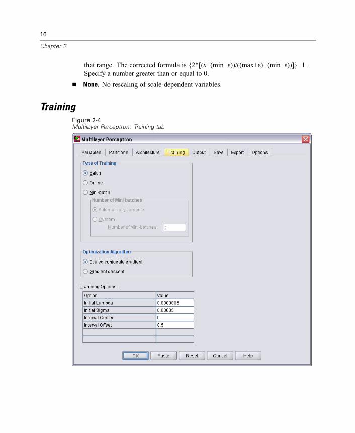
TrainingFigure 2-4Multilayer Perceptron: Training tab
17
Multilayer Perceptron
The Training tab is used to specify how the network should be trained. The type oftraining and the optimization algorithm determine which training options are available.
Type of Training. The training type determines how the network processes the records.Select one of the following training types:
Batch. Updates the synaptic weights only after passing all training data records;that is, batch training uses information from all records in the training dataset.Batch training is often preferred because it directly minimizes the total error;however, batch training may need to update the weights many times until one ofthe stopping rules is met and hence may need many data passes. It is most usefulfor “smaller” datasets.Online. Updates the synaptic weights after every single training data record; thatis, online training uses information from one record at a time. Online trainingcontinuously gets a record and updates the weights until one of the stopping rulesis met. If all the records are used once and none of the stopping rules is met, thenthe process continues by recycling the data records. Online training is superiorto batch for “larger” datasets with associated predictors; that is, if there are manyrecords and many inputs, and their values are not independent of each other, thenonline training can more quickly obtain a reasonable answer than batch training.Mini-batch. Divides the training data records into groups of approximately equalsize, then updates the synaptic weights after passing one group; that is, mini-batchtraining uses information from a group of records. Then the process recycles thedata group if necessary. Mini-batch training offers a compromise between batchand online training, and it may be best for “medium-size” datasets. The procedurecan automatically determine the number of training records per mini-batch, oryou can specify an integer greater than 1 and less than or equal to the maximumnumber of cases to store in memory. You can set the maximum number of cases tostore in memory on the Options tab.
Optimization Algorithm. This is the method used to estimate the synaptic weights.Scaled conjugate gradient. The assumptions that justify the use of conjugategradient methods apply only to batch training types, so this method is not availablefor online or mini-batch training.Gradient descent. This method must be used with online or mini-batch training; itcan also be used with batch training.
18
Chapter 2
Training Options. The training options allow you to fine-tune the optimizationalgorithm. You generally will not need to change these settings unless the networkruns into problems with estimation.
Training options for the scaled conjugate gradient algorithm include:Initial Lambda. The initial value of the lambda parameter for the scaled conjugategradient algorithm. Specify a number greater than 0 and less than 0.000001.Initial Sigma. The initial value of the sigma parameter for the scaled conjugategradient algorithm. Specify a number greater than 0 and less than 0.0001.Interval Center and Interval Offset. The interval center (a0) and interval offset (a)define the interval [a0−a, a0+a], in which weight vectors are randomly generatedwhen simulated annealing is used. Simulated annealing is used to break out of alocal minimum, with the goal of finding the global minimum, during applicationof the optimization algorithm. This approach is used in weight initialization andautomatic architecture selection. Specify a number for the interval center and anumber greater than 0 for the interval offset.
Training options for the gradient descent algorithm include:Initial Learning Rate. The initial value of the learning rate for the gradient descentalgorithm. A higher learning rate means that the network will train faster, possiblyat the cost of becoming unstable. Specify a number greater than 0.Lower Boundary of Learning Rate. The lower boundary on the learning rate for thegradient descent algorithm. This setting applies only to online and mini-batchtraining. Specify a number greater than 0 and less than the initial learning rate.Momentum. The initial momentum parameter for the gradient descent algorithm.The momentum term helps to prevent instabilities caused by a too-high learningrate. Specify a number greater than 0.Learning rate reduction, in Epochs. The number of epochs (p), or data passes of thetraining sample, required to reduce the initial learning rate to the lower boundary ofthe learning rate when gradient descent is used with online or mini-batch training.This gives you control of the learning rate decay factor β = (1/pK)*ln(η0/ηlow),where η0 is the initial learning rate, ηlow is the lower bound on the learning rate,and K is the total number of mini-batches (or the number of training records foronline training) in the training dataset. Specify an integer greater than 0.
19
Multilayer Perceptron
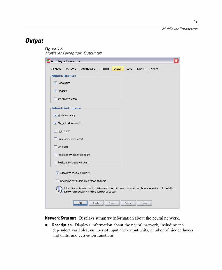
OutputFigure 2-5Multilayer Perceptron: Output tab
Network Structure. Displays summary information about the neural network.Description. Displays information about the neural network, including thedependent variables, number of input and output units, number of hidden layersand units, and activation functions.
20
Chapter 2
Diagram. Displays the network diagram as a non-editable chart. Note that as thenumber of covariates and factor levels increases, the diagram becomes moredifficult to interpret.Synaptic weights. Displays the coefficient estimates that show the relationshipbetween the units in a given layer to the units in the following layer. The synapticweights are based on the training sample even if the active dataset is partitionedinto training, testing, and holdout data. Note that the number of synaptic weightscan become rather large and that these weights are generally not used forinterpreting network results.
Network Performance. Displays results used to determine whether the model is “good”.Note: Charts in this group are based on the combined training and testing samples oronly on the training sample if there is no testing sample.
Model summary. Displays a summary of the neural network results by partitionand overall, including the error, the relative error or percentage of incorrectpredictions, the stopping rule used to stop training, and the training time.The error is the sum-of-squares error when the identity, sigmoid, or hyperbolictangent activation function is applied to the output layer. It is the cross-entropyerror when the softmax activation function is applied to the output layer.Relative errors or percentages of incorrect predictions are displayed depending onthe dependent variable measurement levels. If any dependent variable has scalemeasurement level, then the average overall relative error (relative to the meanmodel) is displayed. If all dependent variables are categorical, then the averagepercentage of incorrect predictions is displayed. Relative errors or percentages ofincorrect predictions are also displayed for individual dependent variables.Classification results. Displays a classification table for each categorical dependentvariable by partition and overall. Each table gives the number of cases classifiedcorrectly and incorrectly for each dependent variable category. The percentage ofthe total cases that were correctly classified is also reported.ROC curve. Displays an ROC (Receiver Operating Characteristic) curve for eachcategorical dependent variable. It also displays a table giving the area under eachcurve. For a given dependent variable, the ROC chart displays one curve for eachcategory. If the dependent variable has two categories, then each curve treats thecategory at issue as the positive state versus the other category. If the dependentvariable has more than two categories, then each curve treats the category at issueas the positive state versus the aggregate of all other categories.
21
Multilayer Perceptron
Cumulative gains chart. Displays a cumulative gains chart for each categoricaldependent variable. The display of one curve for each dependent variable categoryis the same as for ROC curves.Lift chart. Displays a lift chart for each categorical dependent variable. The displayof one curve for each dependent variable category is the same as for ROC curves.Predicted by observed chart. Displays a predicted-by-observed-value chart for eachdependent variable. For categorical dependent variables, clustered boxplots ofpredicted pseudo-probabilities are displayed for each response category, with theobserved response category as the cluster variable. For scale-dependent variables,a scatterplot is displayed.Residual by predicted chart. Displays a residual-by-predicted-value chart for eachscale-dependent variable. There should be no visible patterns between residualsand predicted values. This chart is produced only for scale-dependent variables.
Case processing summary. Displays the case processing summary table, whichsummarizes the number of cases included and excluded in the analysis, in total and bytraining, testing, and holdout samples.
Independent variable importance analysis. Performs a sensitivity analysis, whichcomputes the importance of each predictor in determining the neural network. Theanalysis is based on the combined training and testing samples or only on the trainingsample if there is no testing sample. This creates a table and a chart displayingimportance and normalized importance for each predictor. Note that sensitivityanalysis is computationally expensive and time-consuming if there are large numbersof predictors or cases.
22
Chapter 2
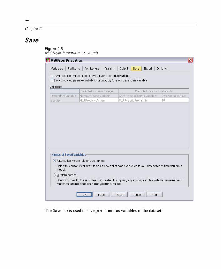
SaveFigure 2-6Multilayer Perceptron: Save tab
The Save tab is used to save predictions as variables in the dataset.
23
Multilayer Perceptron
Save predicted value or category for each dependent variable. This saves thepredicted value for scale-dependent variables and the predicted category forcategorical dependent variables.Save predicted pseudo-probability or category for each dependent variable. Thissaves the predicted pseudo-probabilities for categorical dependent variables. Aseparate variable is saved for each of the first n categories, where n is specified inthe Categories to Save column.
Names of Saved Variables. Automatic name generation ensures that you keep all ofyour work. Custom names allow you to discard/replace results from previous runswithout first deleting the saved variables in the Data Editor.
Probabilities and Pseudo-Probabilities
Categorical dependent variables with softmax activation and cross-entropy error willhave a predicted value for each category, where each predicted value is the probabilitythat the case belongs to the category.Categorical dependent variables with sum-of-squares error will have a predicted
value for each category, but the predicted values cannot be interpreted as probabilities.The procedure saves these predicted pseudo-probabilities even if any are less than 0 orgreater than 1, or the sum for a given dependent variable is not 1.The ROC, cumulative gains, and lift charts (see Output on p. 19) are created based
on pseudo-probabilities. In the event that any of the pseudo-probabilities are less than0 or greater than 1, or the sum for a given variable is not 1, they are first rescaled to bebetween 0 and 1 and to sum to 1. Pseudo-probabilities are rescaled by dividing by theirsum. For example, if a case has predicted pseudo-probabilities of 0.50, 0.60, and 0.40for a three-category dependent variable, then each pseudo-probability is divided bythe sum 1.50 to get 0.33, 0.40, and 0.27.If any of the pseudo-probabilities are negative, then the absolute value of the lowest
is added to all pseudo-probabilities before the above rescaling. For example, if thepseudo-probabilities are -0.30, 0.50, and 1.30, then first add 0.30 to each value to get0.00, 0.80, and 1.60. Next, divide each new value by the sum 2.40 to get 0.00, 0.33,and 0.67.
24
Chapter 2
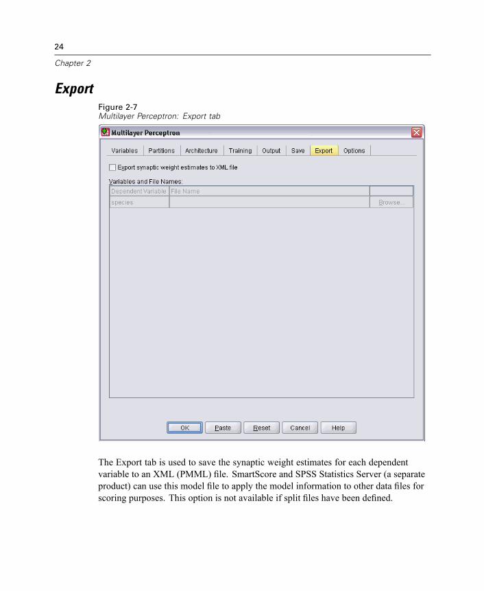
ExportFigure 2-7Multilayer Perceptron: Export tab
The Export tab is used to save the synaptic weight estimates for each dependentvariable to an XML (PMML) file. SmartScore and SPSS Statistics Server (a separateproduct) can use this model file to apply the model information to other data files forscoring purposes. This option is not available if split files have been defined.
25
Multilayer Perceptron
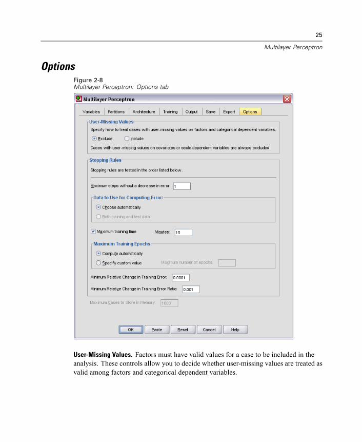
OptionsFigure 2-8Multilayer Perceptron: Options tab
User-Missing Values. Factors must have valid values for a case to be included in theanalysis. These controls allow you to decide whether user-missing values are treated asvalid among factors and categorical dependent variables.
26
Chapter 2
Stopping Rules. These are the rules that determine when to stop training the neuralnetwork. Training proceeds through at least one data pass. Training can then bestopped according to the following criteria, which are checked in the listed order. Inthe stopping rule definitions that follow, a step corresponds to a data pass for the onlineand mini-batch methods and an iteration for the batch method.
Maximum steps without a decrease in error. The number of steps to allow beforechecking for a decrease in error. If there is no decrease in error after the specifiednumber of steps, then training stops. Specify an integer greater than 0. You canalso specify which data sample is used to compute the error. Choose automaticallyuses the testing sample if it exists and uses the training sample otherwise. Notethat batch training guarantees a decrease in the training sample error after eachdata pass; thus, this option applies only to batch training if a testing sample exists.Both training and test data checks the error for each of these samples; this optionapplies only if a testing sample exits.Note: After each complete data pass, online and mini-batch training require anextra data pass in order to compute the training error. This extra data pass can slowtraining considerably, so it is generally recommended that you supply a testingsample and select Choose automatically in any case.Maximum training time. Choose whether to specify a maximum number of minutesfor the algorithm to run. Specify a number greater than 0.Maximum Training Epochs. The maximum number of epochs (data passes) allowed.If the maximum number of epochs is exceeded, then training stops. Specify aninteger greater than 0.Minimum relative change in training error. Training stops if the relative change inthe training error compared to the previous step is less than the criterion value.Specify a number greater than 0. For online and mini-batch training, this criterionis ignored if only testing data is used to compute the error.Minimum relative change in training error ratio. Training stops if the ratio of thetraining error to the error of the null model is less than the criterion value. The nullmodel predicts the average value for all dependent variables. Specify a numbergreater than 0. For online and mini-batch training, this criterion is ignored if onlytesting data is used to compute the error.
Maximum cases to store in memory. This controls the following settings within themultilayer perceptron algorithms. Specify an integer greater than 1.

27
Multilayer Perceptron
In automatic architecture selection, the size of the sample used to determine thenetwork archicteture is min(1000,memsize), where memsize is the maximumnumber of cases to store in memory.In mini-batch training with automatic computation of the number of mini-batches,the number of mini-batches is min(max(M/10,2),memsize), where M is the numberof cases in the training sample.
Chapter
3Radial Basis Function
The Radial Basis Function (RBF) procedure produces a predictive model for one ormore dependent (target) variables based on values of predictor variables.
Example. A telecommunications provider has segmented its customer base by serviceusage patterns, categorizing the customers into four groups. An RBF network usingdemographic data to predict group membership allows the company to customizeoffers for individual prospective customers.
Dependent variables. The dependent variables can be:Nominal. A variable can be treated as nominal when its values represent categorieswith no intrinsic ranking (for example, the department of the company in whichan employee works). Examples of nominal variables include region, zip code,and religious affiliation.Ordinal. A variable can be treated as ordinal when its values represent categorieswith some intrinsic ranking (for example, levels of service satisfaction fromhighly dissatisfied to highly satisfied). Examples of ordinal variables includeattitude scores representing degree of satisfaction or confidence and preferencerating scores.Scale. A variable can be treated as scale when its values represent orderedcategories with a meaningful metric, so that distance comparisons between valuesare appropriate. Examples of scale variables include age in years and incomein thousands of dollars.The procedure assumes that the appropriate measurement level has been assignedto all dependent variables, although you can temporarily change the measurementlevel for a variable by right-clicking the variable in the source variable list andselecting a measurement level from the context menu.
28
29
Radial Basis Function
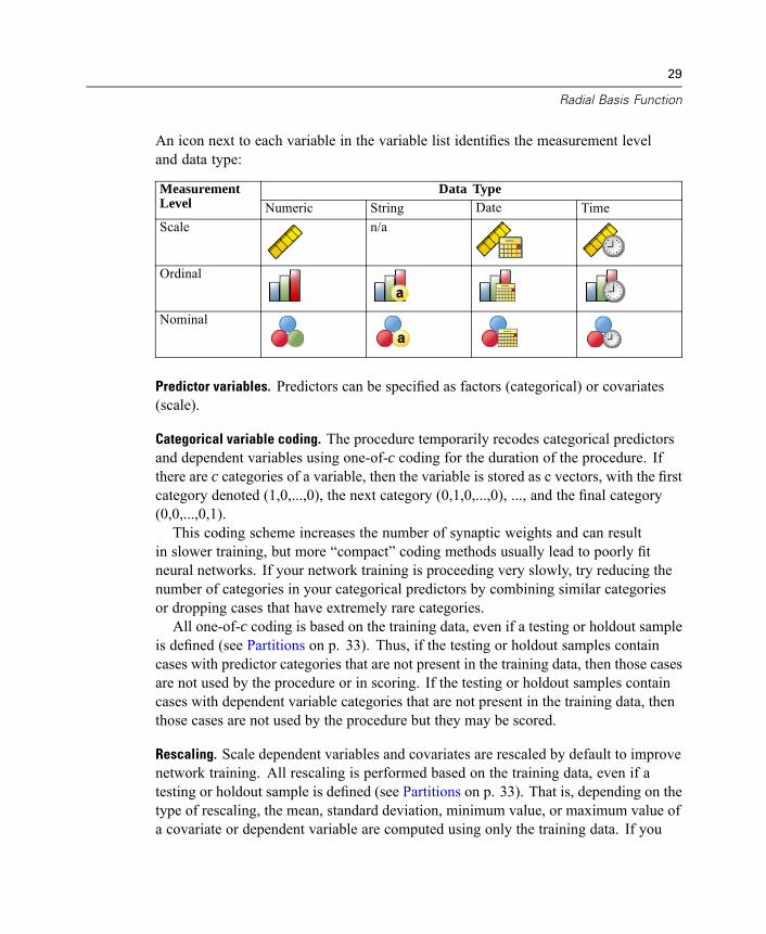
An icon next to each variable in the variable list identifies the measurement leveland data type:
Data TypeMeasurementLevel Numeric String Date TimeScale n/a
Ordinal
Nominal
Predictor variables. Predictors can be specified as factors (categorical) or covariates(scale).
Categorical variable coding. The procedure temporarily recodes categorical predictorsand dependent variables using one-of-c coding for the duration of the procedure. Ifthere are c categories of a variable, then the variable is stored as c vectors, with the firstcategory denoted (1,0,...,0), the next category (0,1,0,...,0), ..., and the final category(0,0,...,0,1).This coding scheme increases the number of synaptic weights and can result
in slower training, but more “compact” coding methods usually lead to poorly fitneural networks. If your network training is proceeding very slowly, try reducing thenumber of categories in your categorical predictors by combining similar categoriesor dropping cases that have extremely rare categories.All one-of-c coding is based on the training data, even if a testing or holdout sample
is defined (see Partitions on p. 33). Thus, if the testing or holdout samples containcases with predictor categories that are not present in the training data, then those casesare not used by the procedure or in scoring. If the testing or holdout samples containcases with dependent variable categories that are not present in the training data, thenthose cases are not used by the procedure but they may be scored.
Rescaling. Scale dependent variables and covariates are rescaled by default to improvenetwork training. All rescaling is performed based on the training data, even if atesting or holdout sample is defined (see Partitions on p. 33). That is, depending on thetype of rescaling, the mean, standard deviation, minimum value, or maximum value ofa covariate or dependent variable are computed using only the training data. If you
30
Chapter 3
specify a variable to define partitions, it is important that these covariates or dependentvariables have similar distributions across the training, testing, and holdout samples.
Frequency weights. Frequency weights are ignored by this procedure.
Replicating results. If you want to exactly replicate your results, use the sameinitialization value for the random number generator and the same data order, inaddition to using the same procedure settings. More details on this issue follow:
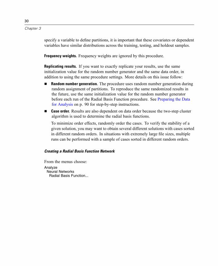
Random number generation. The procedure uses random number generation duringrandom assignment of partitions. To reproduce the same randomized results inthe future, use the same initialization value for the random number generatorbefore each run of the Radial Basis Function procedure. See Preparing the Datafor Analysis on p. 90 for step-by-step instructions.Case order. Results are also dependent on data order because the two-step clusteralgorithm is used to determine the radial basis functions.To minimize order effects, randomly order the cases. To verify the stability of agiven solution, you may want to obtain several different solutions with cases sortedin different random orders. In situations with extremely large file sizes, multipleruns can be performed with a sample of cases sorted in different random orders.
Creating a Radial Basis Function Network
From the menus choose:Analyze
Neural NetworksRadial Basis Function...
31
Radial Basis Function
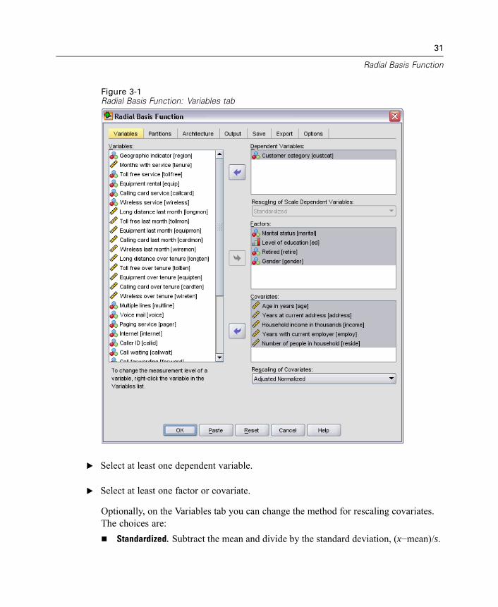
Figure 3-1Radial Basis Function: Variables tab
E Select at least one dependent variable.
E Select at least one factor or covariate.
Optionally, on the Variables tab you can change the method for rescaling covariates.The choices are:
Standardized. Subtract the mean and divide by the standard deviation, (x−mean)/s.

32
Chapter 3
Normalized. Subtract the minimum and divide by the range, (x−min)/(max−min).Normalized values fall between 0 and 1.Adjusted Normalized. Adjusted version of subtracting the minimum and dividingby the range, [2*(x−min)/(max−min)]−1. Adjusted normalized values fall between−1 and 1.None. No rescaling of covariates.
33
Radial Basis Function
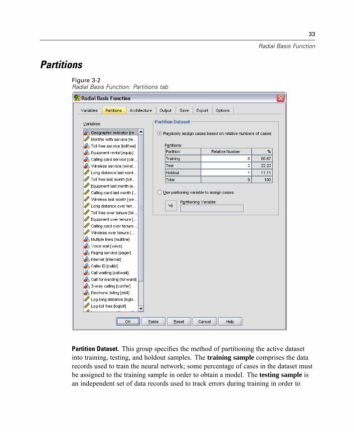
PartitionsFigure 3-2Radial Basis Function: Partitions tab
Partition Dataset. This group specifies the method of partitioning the active datasetinto training, testing, and holdout samples. The training sample comprises the datarecords used to train the neural network; some percentage of cases in the dataset mustbe assigned to the training sample in order to obtain a model. The testing sample isan independent set of data records used to track errors during training in order to
34
Chapter 3
prevent overtraining. It is highly recommended that you create a training sample,and network training will generally be most efficient if the testing sample is smallerthan the training sample. The holdout sample is another independent set of datarecords used to assess the final neural network; the error for the holdout sample givesan “honest” estimate of the predictive ability of the model because the holdout caseswere not used to build the model.
Randomly assign cases based on relative number of cases. Specify the relativenumber (ratio) of cases randomly assigned to each sample (training, testing, andholdout). The % column reports the percentage of cases that will be assigned toeach sample based on the relative numbers you have specified.For example, specifying 7, 3, 0 as the relative numbers for training, testing, andholdout samples corresponds to 70%, 30%, and 0%. Specifying 2, 1, 1 as therelative numbers corresponds to 50%, 25%, and 25%; 1, 1, 1 corresponds todividing the dataset into equal thirds among training, testing, and holdout.Use partitioning variable to assign cases. Specify a numeric variable that assignseach case in the active dataset to the training, testing, or holdout sample. Caseswith a positive value on the variable are assigned to the training sample, cases witha value of 0, to the testing sample, and cases with a negative value, to the holdoutsample. Cases with a system-missing value are excluded from the analysis. Anyuser-missing values for the partition variable are always treated as valid.
35
Radial Basis Function
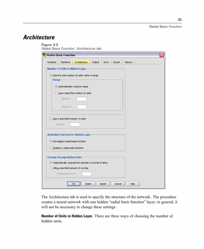
ArchitectureFigure 3-3Radial Basis Function: Architecture tab
The Architecture tab is used to specify the structure of the network. The procedurecreates a neural network with one hidden “radial basis function” layer; in general, itwill not be necessary to change these settings.
Number of Units in Hidden Layer. There are three ways of choosing the number ofhidden units.

36
Chapter 3
1. Find the best number of units within an automatically computed range. The procedureautomatically computes the minimum and maximum values of the range and finds thebest number of hidden units within the range.
If a testing sample is defined, then the procedure uses the testing data criterion: Thebest number of hidden units is the one that yields the smallest error in the testing data.If a testing sample is not defined, then the procedure uses the Bayesian informationcriterion (BIC): The best number of hidden units is the one that yields the smallestBIC based on the training data.
2. Find the best number of units within a specified range. You can provide your own range,and the procedure will find the “best” number of hidden units within that range. Asbefore, the best number of hidden units from the range is determined using the testingdata criterion or the BIC.
3. Use a specified number of units. You can override the use of a range and specify aparticular number of units directly.
Activation Function for Hidden Layer. The activation function for the hidden layer is theradial basis function, which “links” the units in a layer to the values of units in thesucceeding layer. For the output layer, the activation function is the identity function;thus, the output units are simply weighted sums of the hidden units.
Normalized radial basis function. Uses the softmax activation function so theactivations of all hidden units are normalized to sum to 1.Ordinary radial basis function. Uses the exponential activation function so theactivation of the hidden unit is a Gaussian “bump” as a function of the inputs.
Overlap Among Hidden Units. The overlapping factor is a multiplier applied to the widthof the radial basis functions. The automatically computed value of the overlappingfactor is 1+0.1d, where d is the number of input units (the sum of the number ofcategories across all factors and the number of covariates).
37
Radial Basis Function
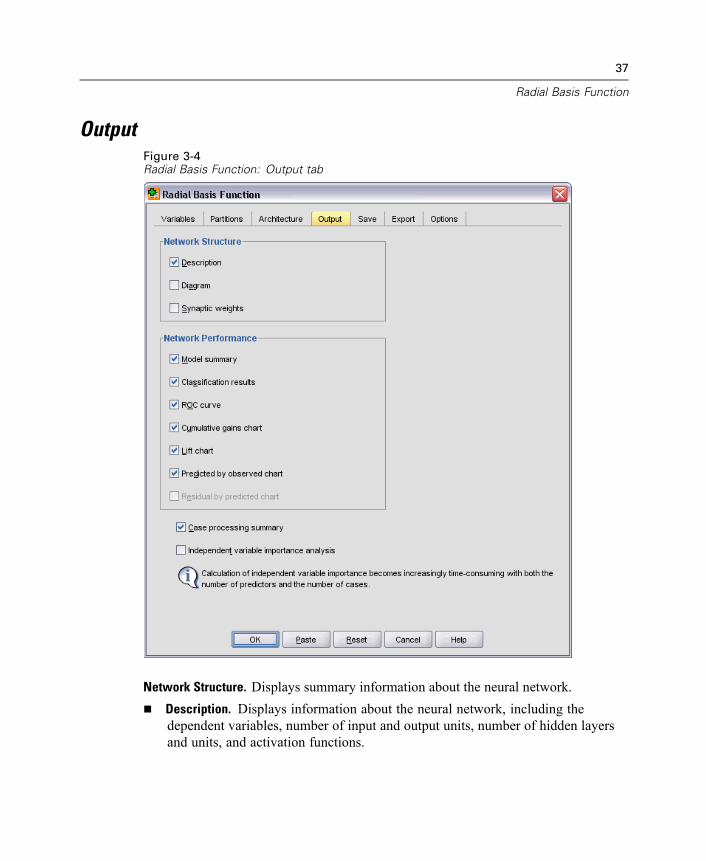
OutputFigure 3-4Radial Basis Function: Output tab
Network Structure. Displays summary information about the neural network.Description. Displays information about the neural network, including thedependent variables, number of input and output units, number of hidden layersand units, and activation functions.
38
Chapter 3
Diagram. Displays the network diagram as a non-editable chart. Note that as thenumber of covariates and factor levels increases, the diagram becomes moredifficult to interpret.Synaptic weights. Displays the coefficient estimates that show the relationshipbetween the units in a given layer to the units in the following layer. The synapticweights are based on the training sample even if the active dataset is partitionedinto training, testing, and holdout data. Note that the number of synaptic weightscan become rather large, and these weights are generally not used for interpretingnetwork results.
Network Performance. Displays results used to determine whether the model is “good.”Note: Charts in this group are based on the combined training and testing samples oronly the training sample if there is no testing sample.
Model summary. Displays a summary of the neural network results by partitionand overall, including the error, the relative error or percentage of incorrectpredictions, and the training time.The error is the sum-of-squares error. In addition, relative errors or percentagesof incorrect predictions are displayed, depending on the dependent variablemeasurement levels. If any dependent variable has scale measurement level, thenthe average overall relative error (relative to the mean model) is displayed. Ifall dependent variables are categorical, then the average percentage of incorrectpredictions is displayed. Relative errors or percentages of incorrect predictionsare also displayed for individual dependent variables.Classification results. Displays a classification table for each categorical dependentvariable. Each table gives the number of cases classified correctly and incorrectlyfor each dependent variable category. The percentage of the total cases that werecorrectly classified is also reported.ROC curve. Displays an ROC (Receiver Operating Characteristic) curve for eachcategorical dependent variable. It also displays a table giving the area under eachcurve. For a given dependent variable, the ROC chart displays one curve for eachcategory. If the dependent variable has two categories, then each curve treats thecategory at issue as the positive state versus the other category. If the dependentvariable has more than two categories, then each curve treats the category at issueas the positive state versus the aggregate of all other categories.Cumulative gains chart. Displays a cumulative gains chart for each categoricaldependent variable. The display of one curve for each dependent variable categoryis the same as for ROC curves.
39
Radial Basis Function
Lift chart. Displays a lift chart for each categorical dependent variable. The displayof one curve for each dependent variable category is the same as for ROC curves.Predicted by observed chart. Displays a predicted-by-observed-value chart for eachdependent variable. For categorical dependent variables, clustered boxplots ofpredicted pseudo-probabilities are displayed for each response category, with theobserved response category as the cluster variable. For scale dependent variables,a scatterplot is displayed.Residual by predicted chart. Displays a residual-by-predicted-value chart for eachscale dependent variable. There should be no visible patterns between residualsand predicted values. This chart is produced only for scale dependent variables.
Case processing summary. Displays the case processing summary table, whichsummarizes the number of cases included and excluded in the analysis, in total and bytraining, testing, and holdout samples.
Independent variable importance analysis. Performs a sensitivity analysis, whichcomputes the importance of each predictor in determining the neural network. Theanalysis is based on the combined training and testing samples or only the trainingsample if there is no testing sample. This creates a table and a chart displayingimportance and normalized importance for each predictor. Note that sensitivityanalysis is computationally expensive and time-consuming if there is a large number ofpredictors or cases.
40
Chapter 3
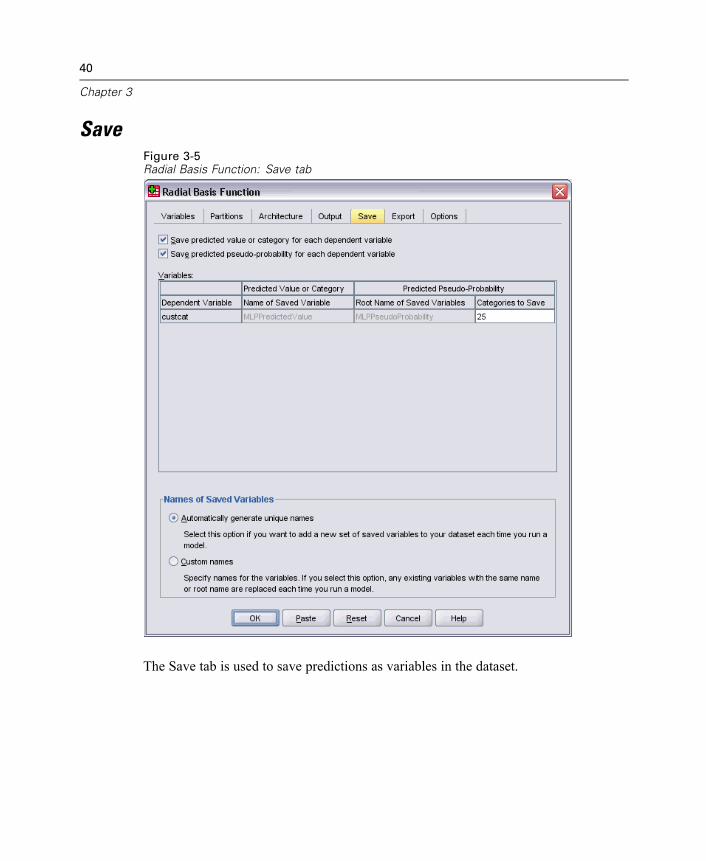
SaveFigure 3-5Radial Basis Function: Save tab
The Save tab is used to save predictions as variables in the dataset.
41
Radial Basis Function
Save predicted value or category for each dependent variable. This saves thepredicted value for scale dependent variables and the predicted category forcategorical dependent variables.Save predicted pseudo-probability for each dependent variable. This saves thepredicted pseudo-probabilities for categorical dependent variables. A separatevariable is saved for each of the first n categories, where n is specified in theCategories to Save column.
Names of Saved Variables. Automatic name generation ensures that you keep all ofyour work. Custom names allow you to discard or replace results from previous runswithout first deleting the saved variables in the Data Editor.
Probabilities and Pseudo-Probabilities
Predicted pseudo-probabilities cannot be interpreted as probabilities because the RadialBasis Function procedure uses the sum-of-squares error and identity activation functionfor the output layer. The procedure saves these predicted pseudo-probabilities even ifany are less than 0 or greater than 1 or the sum for a given dependent variable is not 1.The ROC, cumulative gains, and lift charts (see Output on p. 37) are created based
on pseudo-probabilities. In the event that any of the pseudo-probabilities are less than0 or greater than 1 or the sum for a given variable is not 1, they are first rescaled to bebetween 0 and 1 and to sum to 1. Pseudo-probabilities are rescaled by dividing by theirsum. For example, if a case has predicted pseudo-probabilities of 0.50, 0.60, and 0.40for a three-category dependent variable, then each pseudo-probability is divided bythe sum 1.50 to get 0.33, 0.40, and 0.27.If any of the pseudo-probabilities are negative, then the absolute value of the lowest
is added to all pseudo-probabilities before the above rescaling. For example, if thepseudo-probabilities are –0.30, .50, and 1.30, then first add 0.30 to each value to get0.00, 0.80, and 1.60. Next, divide each new value by the sum 2.40 to get 0.00, 0.33,and 0.67.
42
Chapter 3
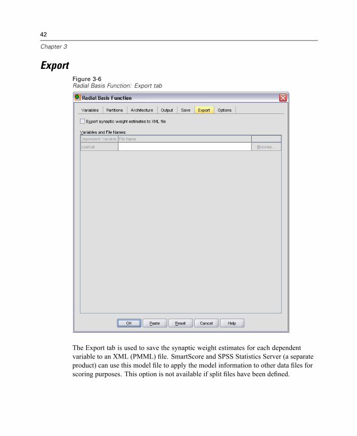
ExportFigure 3-6Radial Basis Function: Export tab
The Export tab is used to save the synaptic weight estimates for each dependentvariable to an XML (PMML) file. SmartScore and SPSS Statistics Server (a separateproduct) can use this model file to apply the model information to other data files forscoring purposes. This option is not available if split files have been defined.
43
Radial Basis Function
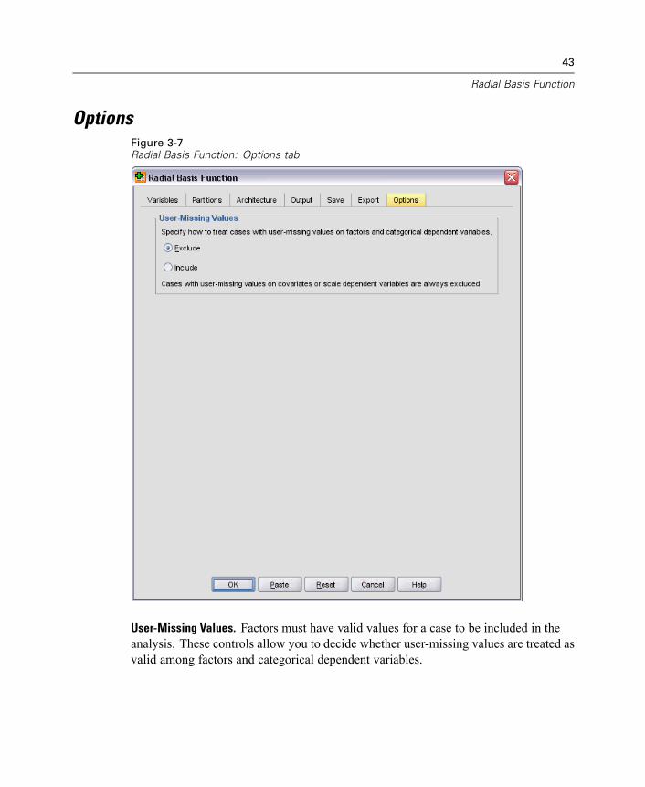
OptionsFigure 3-7Radial Basis Function: Options tab
User-Missing Values. Factors must have valid values for a case to be included in theanalysis. These controls allow you to decide whether user-missing values are treated asvalid among factors and categorical dependent variables.

Part II:Examples
Chapter
4Multilayer Perceptron
The Multilayer Perceptron (MLP) procedure produces a predictive model for one ormore dependent (target) variables based on values of the predictor variables.
Using a Multilayer Perceptron to Assess Credit Risk
A loan officer at a bank needs to be able to identify characteristics that are indicativeof people who are likely to default on loans and use those characteristics to identifygood and bad credit risks.Suppose that information on 850 past and prospective customers is contained in
bankloan.sav. For more information, see Sample Files in Appendix A on p. 108.The first 700 cases are customers who were previously given loans. Use a randomsample of these 700 customers to create a multilayer perceptron, setting the remainingcustomers aside to validate the analysis. Then use the model to classify the 150prospective customers as good or bad credit risks.Additionally, the loan officer has previously analyzed the data using logistic
regression (in the Regression option) and wonders how the multilayer perceptroncompares as a classification tool.
Preparing the Data for Analysis
Setting the random seed allows you to replicate the analysis exactly.
E To set the random seed, from the menus choose:Transform
Random Number Generators...
45
46
Chapter 4
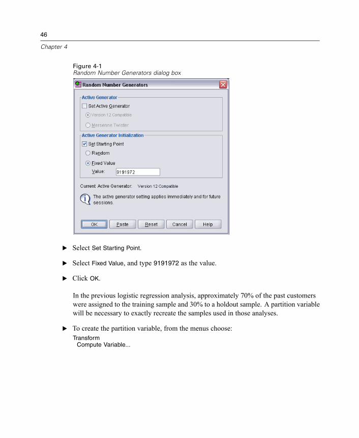
Figure 4-1Random Number Generators dialog box
E Select Set Starting Point.
E Select Fixed Value, and type 9191972 as the value.
E Click OK.
In the previous logistic regression analysis, approximately 70% of the past customerswere assigned to the training sample and 30% to a holdout sample. A partition variablewill be necessary to exactly recreate the samples used in those analyses.
E To create the partition variable, from the menus choose:Transform
Compute Variable...
47
Multilayer Perceptron
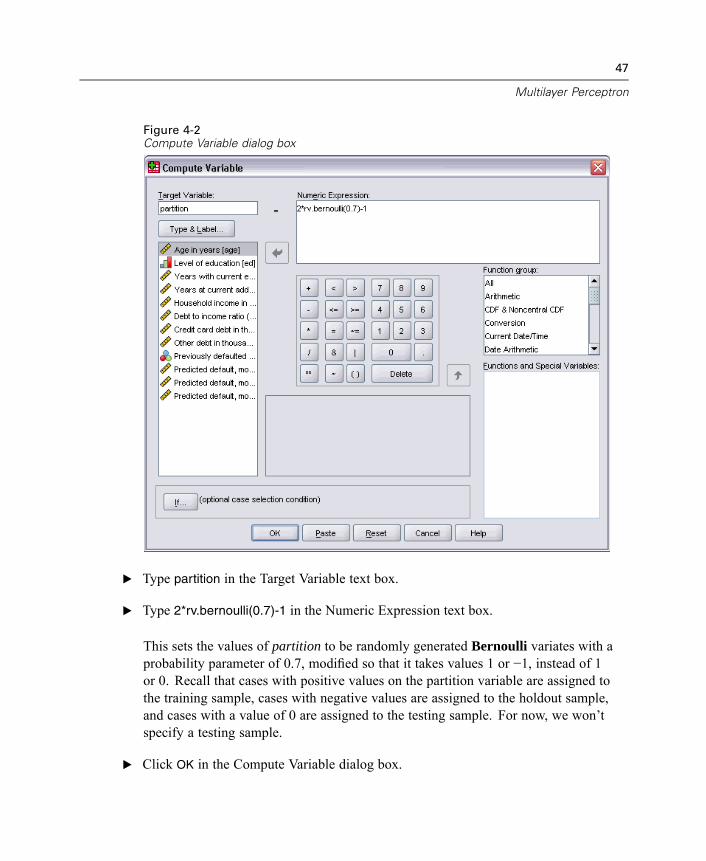
Figure 4-2Compute Variable dialog box
E Type partition in the Target Variable text box.
E Type 2*rv.bernoulli(0.7)-1 in the Numeric Expression text box.
This sets the values of partition to be randomly generated Bernoulli variates with aprobability parameter of 0.7, modified so that it takes values 1 or −1, instead of 1or 0. Recall that cases with positive values on the partition variable are assigned tothe training sample, cases with negative values are assigned to the holdout sample,and cases with a value of 0 are assigned to the testing sample. For now, we won’tspecify a testing sample.
E Click OK in the Compute Variable dialog box.

48
Chapter 4
Approximately 70% of the customers previously given loans will have a partitionvalue of 1. These customers will be used to create the model. The remaining customerswho were previously given loans will have a partition value of −1 and will be used tovalidate the model results.
Running the Analysis
E To run a Multilayer Perceptron analysis, from the menus choose:Analyze
Neural NetworksMultilayer Perceptron...
49
Multilayer Perceptron
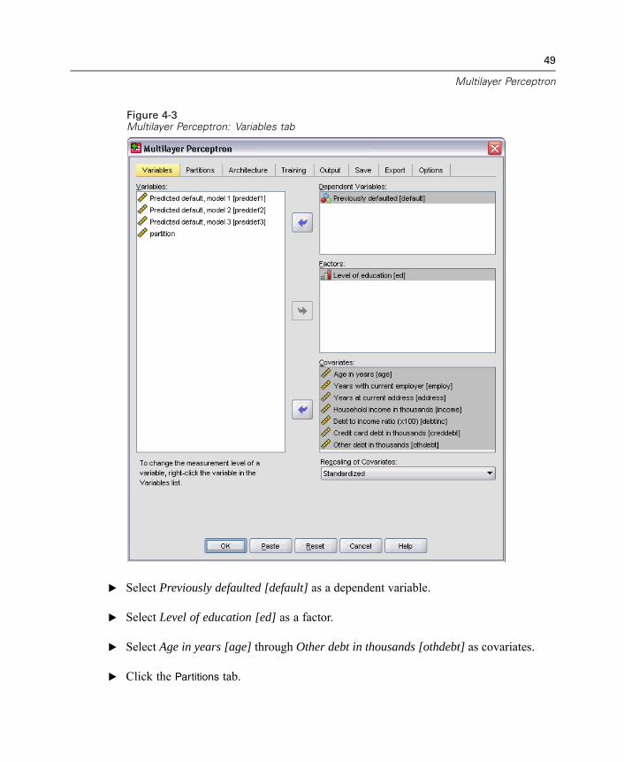
Figure 4-3Multilayer Perceptron: Variables tab
E Select Previously defaulted [default] as a dependent variable.
E Select Level of education [ed] as a factor.
E Select Age in years [age] through Other debt in thousands [othdebt] as covariates.
E Click the Partitions tab.
50
Chapter 4
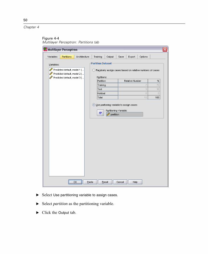
Figure 4-4Multilayer Perceptron: Partitions tab
E Select Use partitioning variable to assign cases.
E Select partition as the partitioning variable.
E Click the Output tab.
51
Multilayer Perceptron
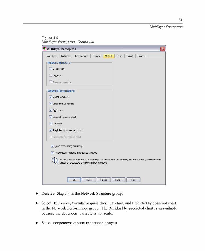
Figure 4-5Multilayer Perceptron: Output tab
E Deselect Diagram in the Network Structure group.
E Select ROC curve, Cumulative gains chart, Lift chart, and Predicted by observed chart
in the Network Performance group. The Residual by predicted chart is unavailablebecause the dependent variable is not scale.
E Select Independent variable importance analysis.
52
Chapter 4
E Click OK.
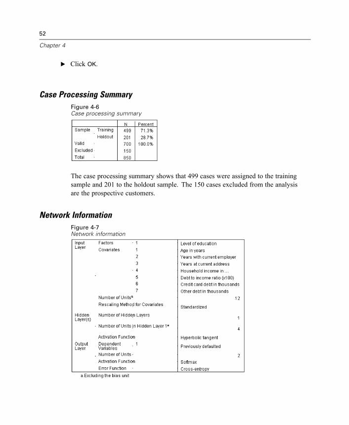
Case Processing SummaryFigure 4-6Case processing summary
The case processing summary shows that 499 cases were assigned to the trainingsample and 201 to the holdout sample. The 150 cases excluded from the analysisare the prospective customers.
Network InformationFigure 4-7Network information

53
Multilayer Perceptron
The network information table displays information about the neural network and isuseful for ensuring that the specifications are correct. Here, note in particular that:
The number of units in the input layer is the number of covariates plus the totalnumber of factor levels; a separate unit is created for each category of Level ofeducation and none of the categories are considered “redundant” units as is typicalin many modeling procedures.Likewise, a separate output unit is created for each category of Previouslydefaulted, for a total of two units in the output layer.Automatic architecture selection has chosen four units in the hidden layer.All other network information is default for the procedure.
Model SummaryFigure 4-8Model summary
The model summary displays information about the results of training and applyingthe final network to the holdout sample.
Cross entropy error is displayed because the output layer uses the softmaxactivation function. This is the error function that the network tries to minimizeduring training.The percentage of incorrect predictions is taken from the classification table andwill be discussed further in that topic.The estimation algorithm stopped because the maximum number of epochs wasreached. Ideally, training should stop because the error has converged. This raisesquestions about whether something went wrong during training and is somethingto keep in mind while further inspecting the output.
54
Chapter 4
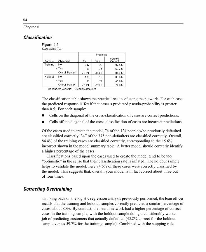
ClassificationFigure 4-9Classification
The classification table shows the practical results of using the network. For each case,the predicted response is Yes if that cases’s predicted pseudo-probability is greaterthan 0.5. For each sample:
Cells on the diagonal of the cross-classification of cases are correct predictions.Cells off the diagonal of the cross-classification of cases are incorrect predictions.
Of the cases used to create the model, 74 of the 124 people who previously defaultedare classified correctly. 347 of the 375 non-defaulters are classified correctly. Overall,84.4% of the training cases are classified correctly, corresponding to the 15.6%incorrect shown in the model summary table. A better model should correctly identifya higher percentage of the cases.Classifications based upon the cases used to create the model tend to be too
“optimistic” in the sense that their classification rate is inflated. The holdout samplehelps to validate the model; here 74.6% of these cases were correctly classified bythe model. This suggests that, overall, your model is in fact correct about three outof four times.
Correcting Overtraining
Thinking back on the logistic regression analysis previously performed, the loan officerrecalls that the training and holdout samples correctly predicted a similar percentage ofcases, about 80%. By contrast, the neural network had a higher percentage of correctcases in the training sample, with the holdout sample doing a considerably worsejob of predicting customers that actually defaulted (45.8% correct for the holdoutsample versus 59.7% for the training sample). Combined with the stopping rule
55
Multilayer Perceptron
reported in the model summary table, this makes you suspect that the network maybe overtraining; that is, it is chasing spurious patterns that appear in the trainingdata by random variation.Fortunately, the solution is relatively simple: specify a testing sample to help keep
the network “on track.” We created the partition variable so that it would exactlyrecreate the training and holdout samples used in the logistic regression analysis;however, logistic regression has no concept of a “testing” sample. Let’s take a portionof the training sample and reassign it to a testing sample.
Creating the Testing Sample
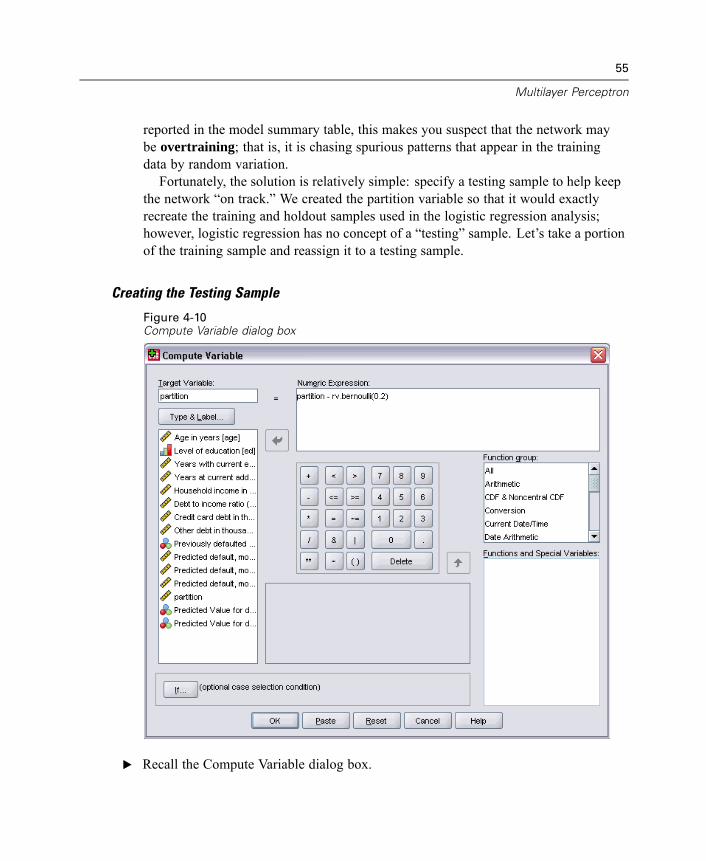
Figure 4-10Compute Variable dialog box
E Recall the Compute Variable dialog box.
56
Chapter 4
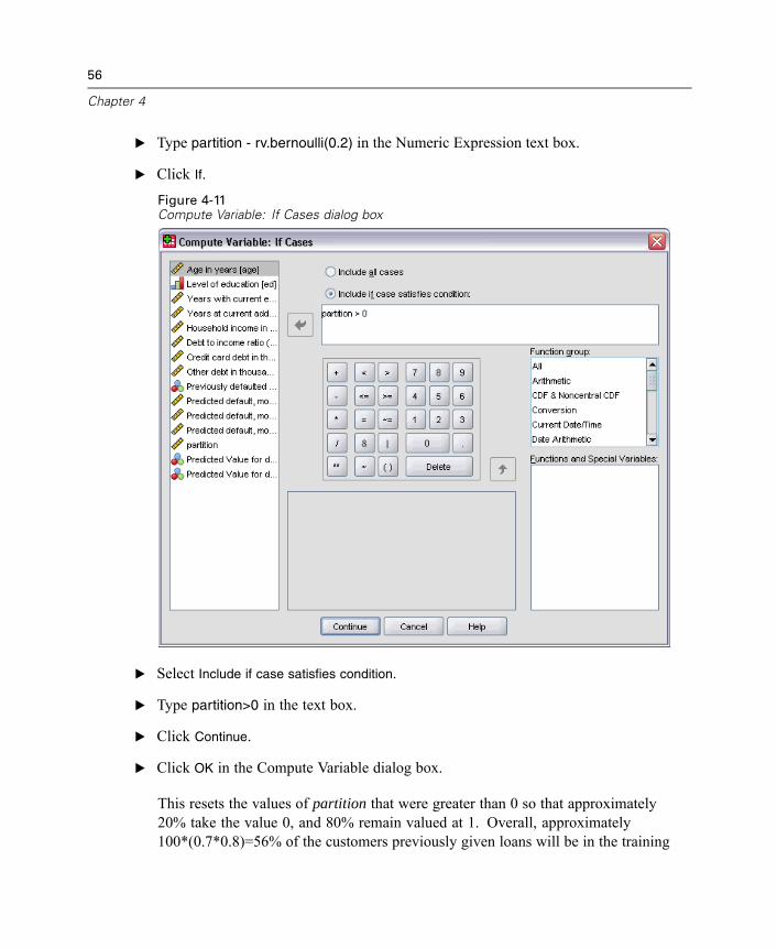
E Type partition - rv.bernoulli(0.2) in the Numeric Expression text box.
E Click If.
Figure 4-11Compute Variable: If Cases dialog box
E Select Include if case satisfies condition.
E Type partition>0 in the text box.
E Click Continue.
E Click OK in the Compute Variable dialog box.
This resets the values of partition that were greater than 0 so that approximately20% take the value 0, and 80% remain valued at 1. Overall, approximately100*(0.7*0.8)=56% of the customers previously given loans will be in the training
57
Multilayer Perceptron
sample, and 14% will be in the testing sample. Customers who were originallyassigned to the holdout sample remain there.
Running the Analysis
E Recall the Multilayer Perceptron dialog box and click the Save tab.
E Select Save predicted pseudo-probability for each dependent variable.
E Click OK.
Case Processing Summary
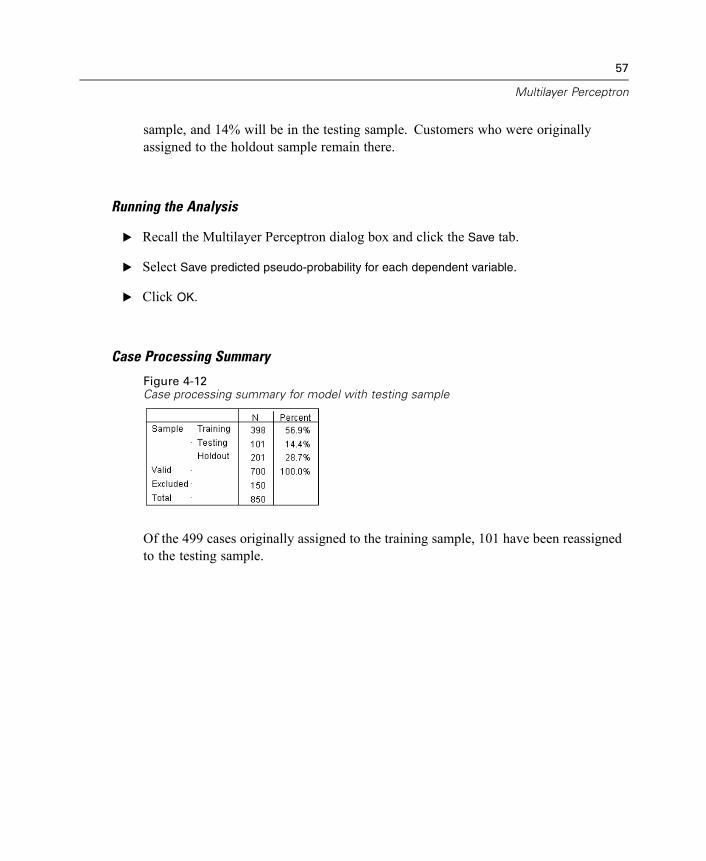
Figure 4-12Case processing summary for model with testing sample
Of the 499 cases originally assigned to the training sample, 101 have been reassignedto the testing sample.
58
Chapter 4
Network Information
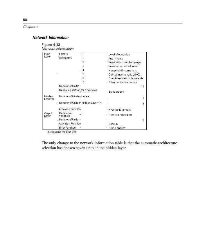
Figure 4-13Network information
The only change to the network information table is that the automatic architectureselection has chosen seven units in the hidden layer.
59
Multilayer Perceptron
Model Summary
Figure 4-14Model summary
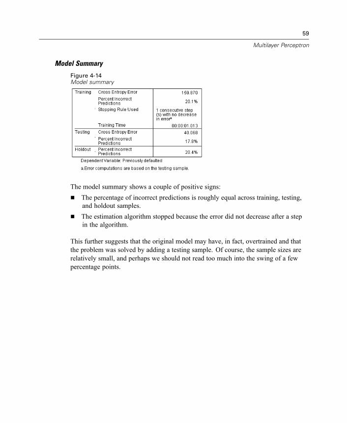
The model summary shows a couple of positive signs:The percentage of incorrect predictions is roughly equal across training, testing,and holdout samples.The estimation algorithm stopped because the error did not decrease after a stepin the algorithm.
This further suggests that the original model may have, in fact, overtrained and thatthe problem was solved by adding a testing sample. Of course, the sample sizes arerelatively small, and perhaps we should not read too much into the swing of a fewpercentage points.
60
Chapter 4
Classification
Figure 4-15Classification
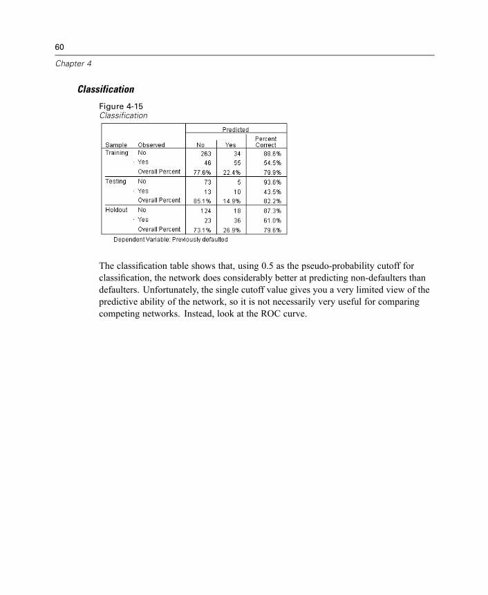
The classification table shows that, using 0.5 as the pseudo-probability cutoff forclassification, the network does considerably better at predicting non-defaulters thandefaulters. Unfortunately, the single cutoff value gives you a very limited view of thepredictive ability of the network, so it is not necessarily very useful for comparingcompeting networks. Instead, look at the ROC curve.
61
Multilayer Perceptron
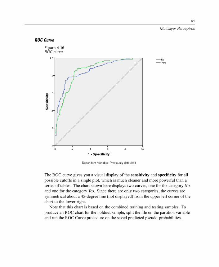
ROC Curve
Figure 4-16ROC curve
The ROC curve gives you a visual display of the sensitivity and specificity for allpossible cutoffs in a single plot, which is much cleaner and more powerful than aseries of tables. The chart shown here displays two curves, one for the category Noand one for the category Yes. Since there are only two categories, the curves aresymmetrical about a 45-degree line (not displayed) from the upper left corner of thechart to the lower right.Note that this chart is based on the combined training and testing samples. To
produce an ROC chart for the holdout sample, split the file on the partition variableand run the ROC Curve procedure on the saved predicted pseudo-probabilities.

62
Chapter 4
Figure 4-17Area under the curve
The area under the curve is a numerical summary of the ROC curve, and thevalues in the table represent, for each category, the probability that the predictedpseudo-probability of being in that category is higher for a randomly chosen case inthat category than for a randomly chosen case not in that category. For example, fora randomly selected defaulter and randomly selected non-defaulter, there is a 0.853probability that the model-predicted pseudo-probability of default will be higher forthe defaulter than for the non-defaulter.While the area under the curve is a useful one-statistic summary of the accuracy of
the network, you need to be able to choose a specific criterion by which customers areclassified. The predicted-by-observed chart provides a visual start on this process.
63
Multilayer Perceptron
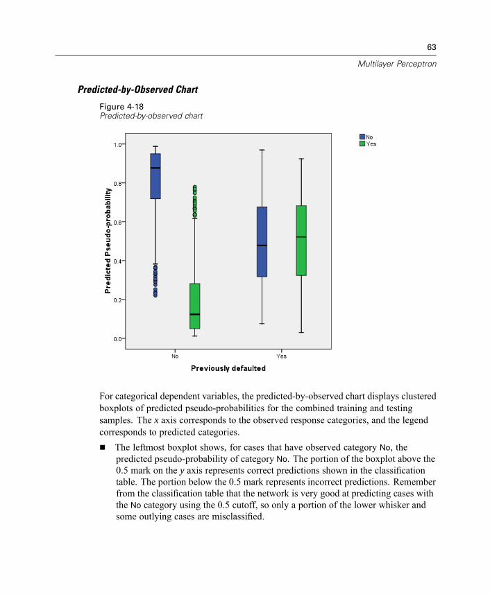
Predicted-by-Observed Chart
Figure 4-18Predicted-by-observed chart
For categorical dependent variables, the predicted-by-observed chart displays clusteredboxplots of predicted pseudo-probabilities for the combined training and testingsamples. The x axis corresponds to the observed response categories, and the legendcorresponds to predicted categories.
The leftmost boxplot shows, for cases that have observed category No, thepredicted pseudo-probability of category No. The portion of the boxplot above the0.5 mark on the y axis represents correct predictions shown in the classificationtable. The portion below the 0.5 mark represents incorrect predictions. Rememberfrom the classification table that the network is very good at predicting cases withthe No category using the 0.5 cutoff, so only a portion of the lower whisker andsome outlying cases are misclassified.

64
Chapter 4
The next boxplot to the right shows, for cases that have observed category No, thepredicted pseudo-probability of category Yes. Since there are only two categoriesin the target variable, the first two boxplots are symmetrical about the horizontalline at 0.5.The third boxplot shows, for cases that have observed category Yes, the predictedpseudo-probability of category No. It and the last boxplot are symmetrical aboutthe horizontal line at 0.5.The last boxplot shows, for cases that have observed category Yes, the predictedpseudo-probability of category Yes. The portion of the boxplot above the 0.5 markon the y axis represents correct predictions shown in the classification table. Theportion below the 0.5 mark represents incorrect predictions. Remember fromthe classification table that the network predicts slightly more than half of thecases with the Yes category using the 0.5 cutoff, so a good portion of the box ismisclassified.
Looking at the plot, it appears that by lowering the cutoff for classifying a case as Yes
from 0.5 to approximately 0.3—this is roughly the value where the top of the secondbox and the bottom of the fourth box are—you can increase the chance of correctlycatching prospective defaulters without losing many potential good customers. Thatis, moving from 0.5 to 0.3 along the second box incorrectly reclassifies relatively fewnon-defaulting customers along the whisker as predicted defaulters, while along thefourth box, this move correctly reclassifies many defaulting customers within the boxas predicted defaulters.
65
Multilayer Perceptron
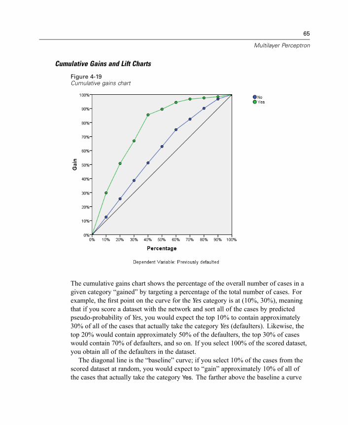
Cumulative Gains and Lift Charts
Figure 4-19Cumulative gains chart
The cumulative gains chart shows the percentage of the overall number of cases in agiven category “gained” by targeting a percentage of the total number of cases. Forexample, the first point on the curve for the Yes category is at (10%, 30%), meaningthat if you score a dataset with the network and sort all of the cases by predictedpseudo-probability of Yes, you would expect the top 10% to contain approximately30% of all of the cases that actually take the category Yes (defaulters). Likewise, thetop 20% would contain approximately 50% of the defaulters, the top 30% of caseswould contain 70% of defaulters, and so on. If you select 100% of the scored dataset,you obtain all of the defaulters in the dataset.The diagonal line is the “baseline” curve; if you select 10% of the cases from the
scored dataset at random, you would expect to “gain” approximately 10% of all ofthe cases that actually take the category Yes. The farther above the baseline a curve
66
Chapter 4
lies, the greater the gain. You can use the cumulative gains chart to help choose aclassification cutoff by choosing a percentage that corresponds to a desirable gain, andthen mapping that percentage to the appropriate cutoff value.What constitutes a “desirable” gain depends on the cost of Type I and Type II errors.
That is, what is the cost of classifying a defaulter as a non-defaulter (Type I)? What isthe cost of classifying a non-defaulter as a defaulter (Type II)? If bad debt is the primaryconcern, then you want to lower your Type I error; on the cumulative gains chart, thismight correspond to rejecting loans to applicants in the top 40% of pseudo-predictedprobability of Yes, which captures nearly 90% of the possible defaulters but removesnearly half of your applicant pool. If growing your customer base is the priority, thenyou want to lower your Type II error. On the chart, this might correspond to rejectingthe top 10%, which captures 30% of the defaulters and leaves most of your applicantpool intact. Usually, both are major concerns, so you have to choose a decision rule forclassifying customers that gives the best mix of sensitivity and specificity.
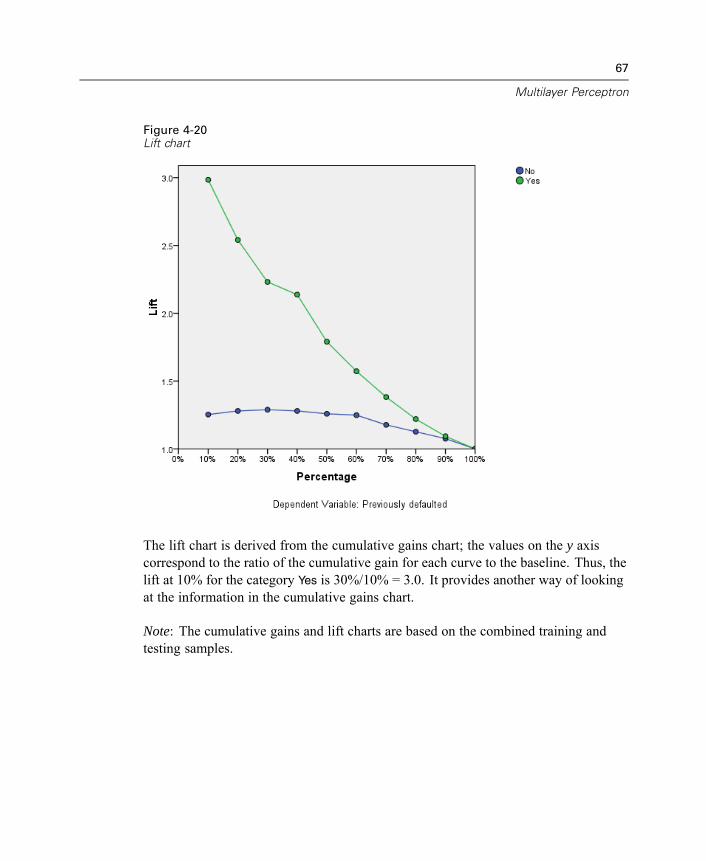
67
Multilayer Perceptron
Figure 4-20Lift chart
The lift chart is derived from the cumulative gains chart; the values on the y axiscorrespond to the ratio of the cumulative gain for each curve to the baseline. Thus, thelift at 10% for the category Yes is 30%/10% = 3.0. It provides another way of lookingat the information in the cumulative gains chart.
Note: The cumulative gains and lift charts are based on the combined training andtesting samples.
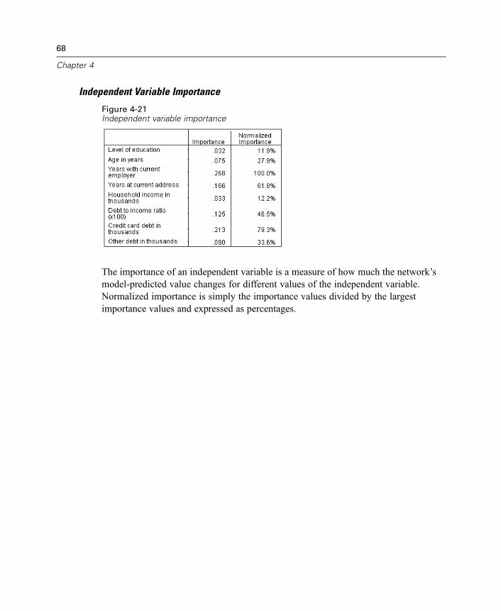
68
Chapter 4
Independent Variable Importance
Figure 4-21Independent variable importance
The importance of an independent variable is a measure of how much the network’smodel-predicted value changes for different values of the independent variable.Normalized importance is simply the importance values divided by the largestimportance values and expressed as percentages.
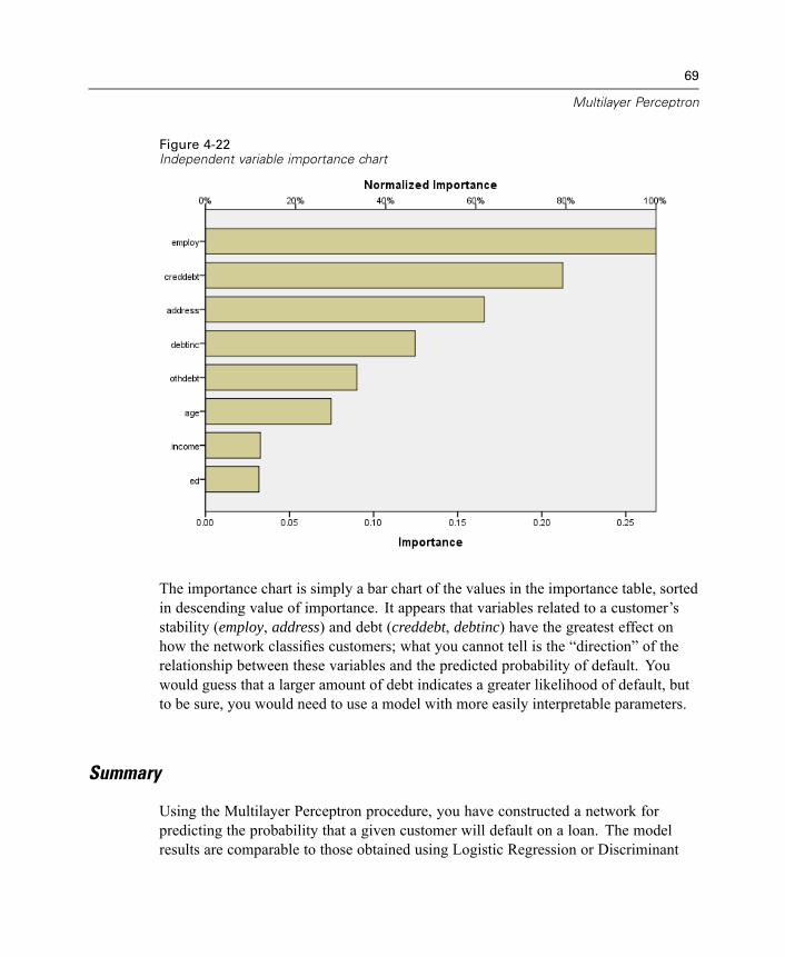
69
Multilayer Perceptron
Figure 4-22Independent variable importance chart
The importance chart is simply a bar chart of the values in the importance table, sortedin descending value of importance. It appears that variables related to a customer’sstability (employ, address) and debt (creddebt, debtinc) have the greatest effect onhow the network classifies customers; what you cannot tell is the “direction” of therelationship between these variables and the predicted probability of default. Youwould guess that a larger amount of debt indicates a greater likelihood of default, butto be sure, you would need to use a model with more easily interpretable parameters.
Summary
Using the Multilayer Perceptron procedure, you have constructed a network forpredicting the probability that a given customer will default on a loan. The modelresults are comparable to those obtained using Logistic Regression or Discriminant
70
Chapter 4
Analysis, so you can be reasonably confident that the data do not contain relationshipsthat cannot be captured by those models; thus, you can use them to further explore thenature of the relationship between the dependent and independent variables.
Using a Multilayer Perceptron to Estimate Healthcare Costsand Lengths of Stay
A hospital system is interested in tracking costs and lengths of stay for patientsadmitted for treatment of myocardial infarction (MI, or “heart attack”). Obtainingaccurate estimates of these measures allow the administration to properly manage theavailable bed space as patients are treated.The data file patient_los.sav contains the treatment records of a sample of patients
who received treatment for MI. For more information, see Sample Files in Appendix Aon p. 108. Use the Multilayer Perceptron procedure to build a network for predictingcosts and length of stay.
Preparing the Data for Analysis
Setting the random seed allows you to replicate the analysis exactly.
E To set the random seed, from the menus choose:Transform
Random Number Generators...

71
Multilayer Perceptron
Figure 4-23Random Number Generators dialog box
E Select Set Starting Point.
E Select Fixed Value, and type 9191972 as the value.
E Click OK.
Running the Analysis
E To run a Multilayer Perceptron analysis, from the menus choose:Analyze
Neural NetworksMultilayer Perceptron...
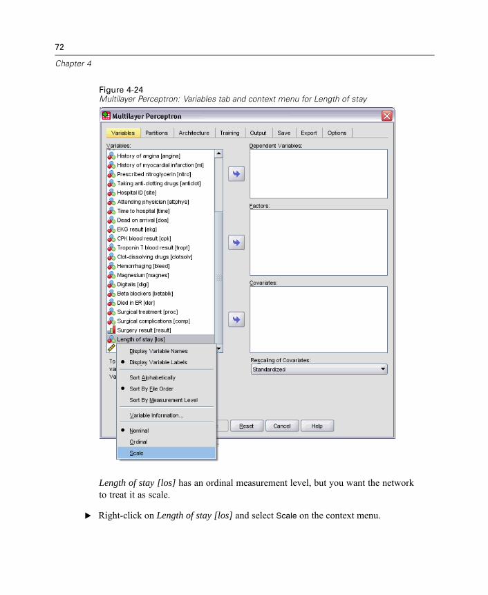
72
Chapter 4
Figure 4-24Multilayer Perceptron: Variables tab and context menu for Length of stay
Length of stay [los] has an ordinal measurement level, but you want the networkto treat it as scale.
E Right-click on Length of stay [los] and select Scale on the context menu.
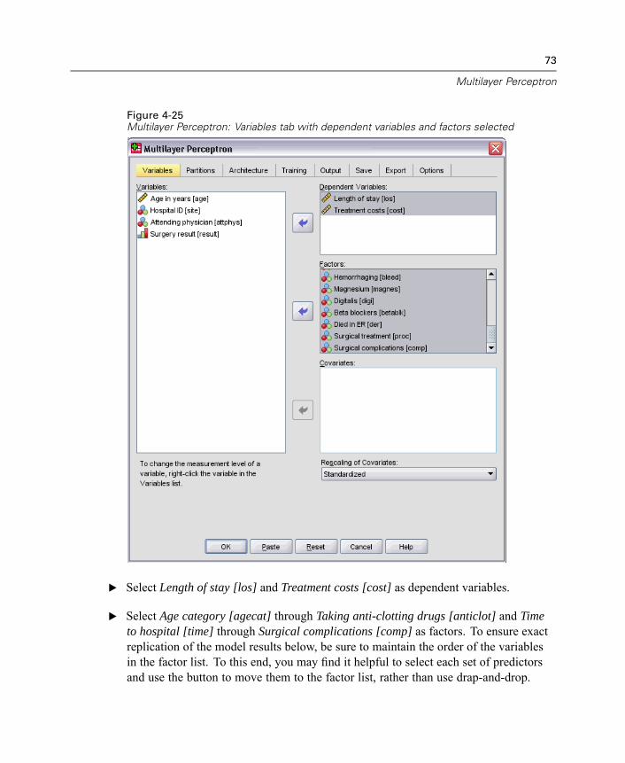
73
Multilayer Perceptron
Figure 4-25Multilayer Perceptron: Variables tab with dependent variables and factors selected
E Select Length of stay [los] and Treatment costs [cost] as dependent variables.
E Select Age category [agecat] through Taking anti-clotting drugs [anticlot] and Timeto hospital [time] through Surgical complications [comp] as factors. To ensure exactreplication of the model results below, be sure to maintain the order of the variablesin the factor list. To this end, you may find it helpful to select each set of predictorsand use the button to move them to the factor list, rather than use drap-and-drop.
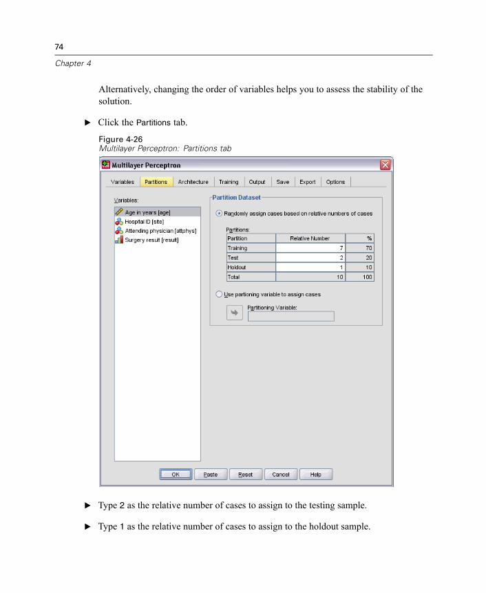
74
Chapter 4
Alternatively, changing the order of variables helps you to assess the stability of thesolution.
E Click the Partitions tab.
Figure 4-26Multilayer Perceptron: Partitions tab
E Type 2 as the relative number of cases to assign to the testing sample.
E Type 1 as the relative number of cases to assign to the holdout sample.
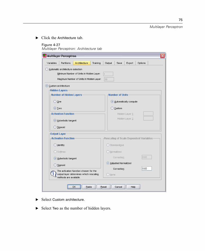
75
Multilayer Perceptron
E Click the Architecture tab.
Figure 4-27Multilayer Perceptron: Architecture tab
E Select Custom architecture.
E Select Two as the number of hidden layers.

76
Chapter 4
E Select Hyperbolic tangent as the output layer activation function. Note that thisautomatically sets the rescaling method for the dependent variables to Adjusted
Normalized.
E Click the Training tab.
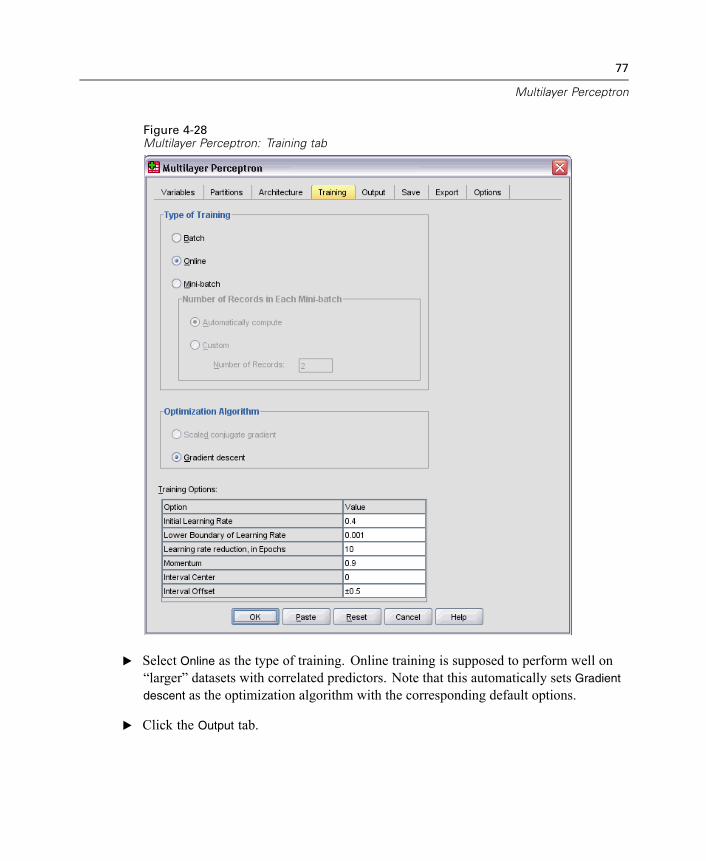
77
Multilayer Perceptron
Figure 4-28Multilayer Perceptron: Training tab
E Select Online as the type of training. Online training is supposed to perform well on“larger” datasets with correlated predictors. Note that this automatically sets Gradient
descent as the optimization algorithm with the corresponding default options.
E Click the Output tab.
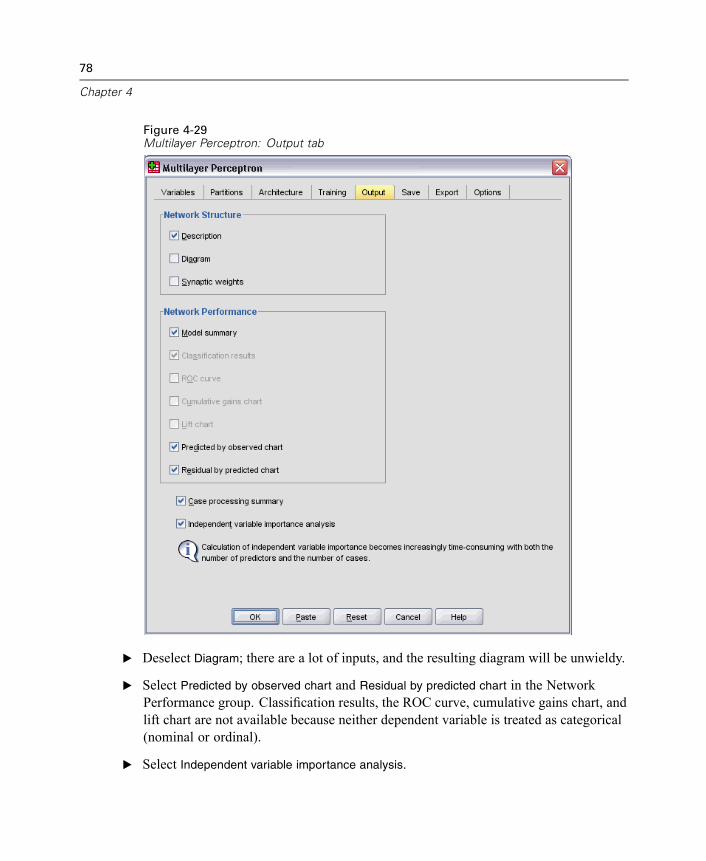
78
Chapter 4
Figure 4-29Multilayer Perceptron: Output tab
E Deselect Diagram; there are a lot of inputs, and the resulting diagram will be unwieldy.
E Select Predicted by observed chart and Residual by predicted chart in the NetworkPerformance group. Classification results, the ROC curve, cumulative gains chart, andlift chart are not available because neither dependent variable is treated as categorical(nominal or ordinal).
E Select Independent variable importance analysis.
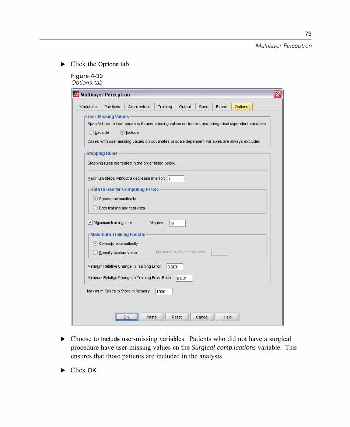
79
Multilayer Perceptron
E Click the Options tab.
Figure 4-30Options tab
E Choose to Include user-missing variables. Patients who did not have a surgicalprocedure have user-missing values on the Surgical complications variable. Thisensures that those patients are included in the analysis.
E Click OK.

80
Chapter 4
WarningsFigure 4-31Warnings
The warnings table notes that the variables doa and der are constant in the trainingsample. Patients who were dead on arrival or died in the emergency room haveuser-missing values on Length of stay. Since we are treating Length of stay as a scalevariable for this analysis and cases with user-missing values on scale variables areexcluded, only patients who lived past the emergency room are included.
Case Processing SummaryFigure 4-32Case processing summary
The case processing summary shows that 5647 cases were assigned to the trainingsample, 1570 to the testing sample, and 781 to the holdout sample. The 2002 casesexcluded from the analysis are patients who died in transit to the hospital or in theemergency room.
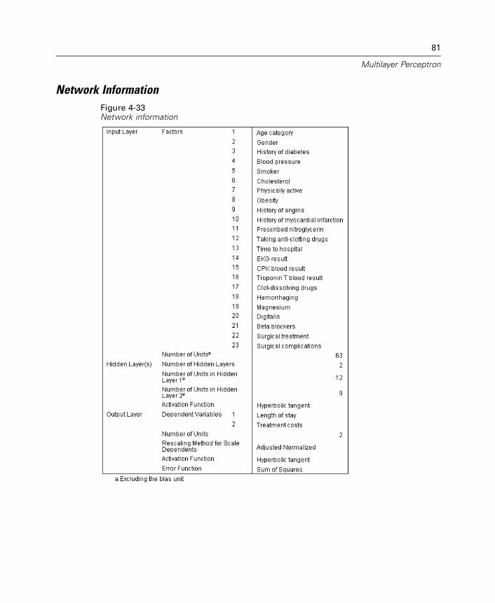
81
Multilayer Perceptron
Network InformationFigure 4-33Network information
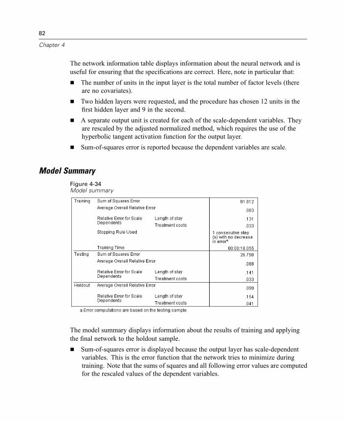
82
Chapter 4
The network information table displays information about the neural network and isuseful for ensuring that the specifications are correct. Here, note in particular that:
The number of units in the input layer is the total number of factor levels (thereare no covariates).Two hidden layers were requested, and the procedure has chosen 12 units in thefirst hidden layer and 9 in the second.A separate output unit is created for each of the scale-dependent variables. Theyare rescaled by the adjusted normalized method, which requires the use of thehyperbolic tangent activation function for the output layer.Sum-of-squares error is reported because the dependent variables are scale.
Model SummaryFigure 4-34Model summary
The model summary displays information about the results of training and applyingthe final network to the holdout sample.
Sum-of-squares error is displayed because the output layer has scale-dependentvariables. This is the error function that the network tries to minimize duringtraining. Note that the sums of squares and all following error values are computedfor the rescaled values of the dependent variables.
83
Multilayer Perceptron
The relative error for each scale-dependent variable is the ratio of thesum-of-squares error for the dependent variable to the sum-of-squares error for the“null” model, in which the mean value of the dependent variable is used as thepredicted value for each case. There appears to be more error in the predictions ofLength of stay than in Treatment costs.The average overall error is the ratio of the sum-of-squares error for all dependentvariables to the sum-of-squares error for the “null” model, in which the meanvalues of the dependent variables are used as the predicted values for each case. Inthis example, the average overall error happens to be close to the average of therelative errors, but this will not always be the case.The average overall relative error and relative errors are fairly constant across thetraining, testing, and holdout samples, which gives you some confidence that themodel is not overtrained and that the error in future cases scored by the networkwill be close to the error reported in this table.The estimation algorithm stopped because the error did not decrease after a stepin the algorithm.
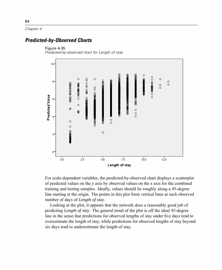
84
Chapter 4
Predicted-by-Observed ChartsFigure 4-35Predicted-by-observed chart for Length of stay
For scale-dependent variables, the predicted-by-observed chart displays a scatterplotof predicted values on the y axis by observed values on the x axis for the combinedtraining and testing samples. Ideally, values should lie roughly along a 45-degreeline starting at the origin. The points in this plot form vertical lines at each observednumber of days of Length of stay.Looking at the plot, it appears that the network does a reasonably good job of
predicting Length of stay. The general trend of the plot is off the ideal 45-degreeline in the sense that predictions for observed lengths of stay under five days tend tooverestimate the length of stay, while predictions for observed lengths of stay beyondsix days tend to underestimate the length of stay.
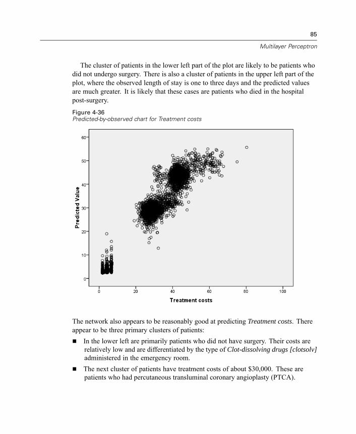
85
Multilayer Perceptron
The cluster of patients in the lower left part of the plot are likely to be patients whodid not undergo surgery. There is also a cluster of patients in the upper left part of theplot, where the observed length of stay is one to three days and the predicted valuesare much greater. It is likely that these cases are patients who died in the hospitalpost-surgery.
Figure 4-36Predicted-by-observed chart for Treatment costs
The network also appears to be reasonably good at predicting Treatment costs. Thereappear to be three primary clusters of patients:
In the lower left are primarily patients who did not have surgery. Their costs arerelatively low and are differentiated by the type of Clot-dissolving drugs [clotsolv]administered in the emergency room.The next cluster of patients have treatment costs of about $30,000. These arepatients who had percutaneous transluminal coronary angioplasty (PTCA).
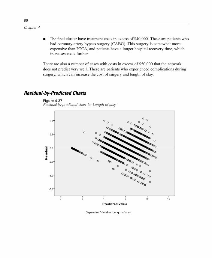
86
Chapter 4
The final cluster have treatment costs in excess of $40,000. These are patients whohad coronary artery bypass surgery (CABG). This surgery is somewhat moreexpensive than PTCA, and patients have a longer hospital recovery time, whichincreases costs further.
There are also a number of cases with costs in excess of $50,000 that the networkdoes not predict very well. These are patients who experienced complications duringsurgery, which can increase the cost of surgery and length of stay.
Residual-by-Predicted ChartsFigure 4-37Residual-by-predicted chart for Length of stay
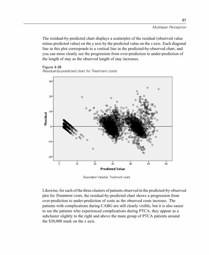
87
Multilayer Perceptron
The residual-by-predicted chart displays a scatterplot of the residual (observed valueminus predicted value) on the y axis by the predicted value on the x axis. Each diagonalline in this plot corresponds to a vertical line in the predicted-by-observed chart, andyou can more clearly see the progression from over-prediction to under-prediction ofthe length of stay as the observed length of stay increases.
Figure 4-38Residual-by-predicted chart for Treatment costs
Likewise, for each of the three clusters of patients observed in the predicted-by-observedplot for Treatment costs, the residual-by-predicted chart shows a progression fromover-prediction to under-prediction of costs as the observed costs increase. Thepatients with complications during CABG are still clearly visible, but it is also easierto see the patients who experienced complications during PTCA; they appear as asubcluster slightly to the right and above the main group of PTCA patients aroundthe $30,000 mark on the x axis.
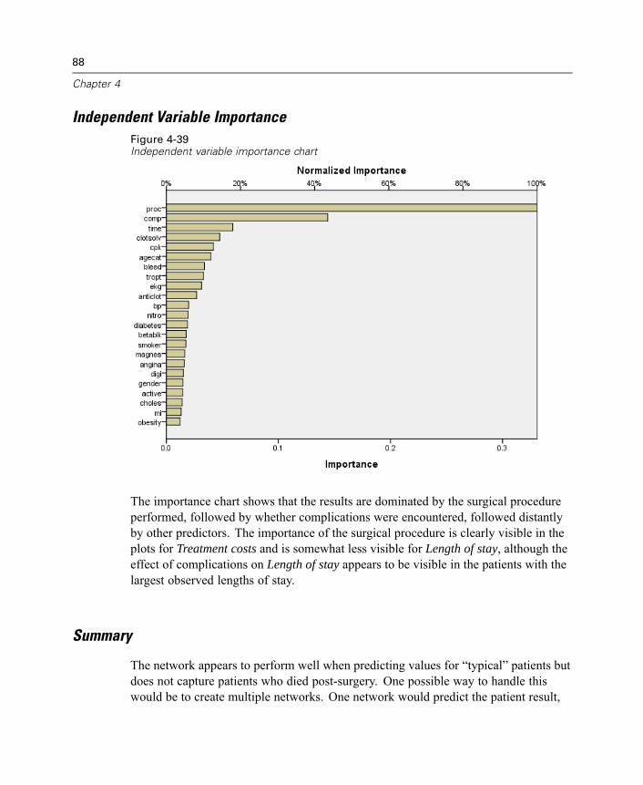
88
Chapter 4
Independent Variable ImportanceFigure 4-39Independent variable importance chart
The importance chart shows that the results are dominated by the surgical procedureperformed, followed by whether complications were encountered, followed distantlyby other predictors. The importance of the surgical procedure is clearly visible in theplots for Treatment costs and is somewhat less visible for Length of stay, although theeffect of complications on Length of stay appears to be visible in the patients with thelargest observed lengths of stay.
Summary
The network appears to perform well when predicting values for “typical” patients butdoes not capture patients who died post-surgery. One possible way to handle thiswould be to create multiple networks. One network would predict the patient result,

89
Multilayer Perceptron
perhaps simply whether the patient survived or not, and then separate networks wouldpredict Treatment costs and Length of stay conditional on whether the patient survived.You could then combine the network results to likely obtain better predictions. Youcould take a similar approach to the problem of under-prediction of costs and lengthsof stay for patients who experienced complications during surgery.
Recommended Readings
See the following texts for more information on neural networks and multilayerperceptrons:
Bishop, C. M. 1995. Neural Networks for Pattern Recognition, 3rd ed. Oxford:Oxford University Press.
Fine, T. L. 1999. Feedforward Neural Network Methodology, 3rd ed. New York:Springer-Verlag.
Haykin, S. 1998. Neural Networks: A Comprehensive Foundation, 2nd ed. New York:Macmillan College Publishing.
Ripley, B. D. 1996. Pattern Recognition and Neural Networks. Cambridge:Cambridge University Press.

Chapter
5Radial Basis Function
The Radial Basis Function (RBF) procedure produces a predictive model for one ormore dependent (target) variables based on values of predictor variables.
Using Radial Basis Function to Classify TelecommunicationsCustomers
A telecommunications provider has segmented its customer base by service usagepatterns, categorizing the customers into four groups. If demographic data can be usedto predict group membership, you can customize offers for individual prospectivecustomers.Suppose information on current customers is contained in telco.sav. For more
information, see Sample Files in Appendix A on p. 108. Use the Radial Basis Functionprocedure to classify customers.
Preparing the Data for Analysis
Setting the random seed allows you to replicate the analysis exactly.
E To set the random seed, from the menus choose:Transform
Random Number Generators...
90
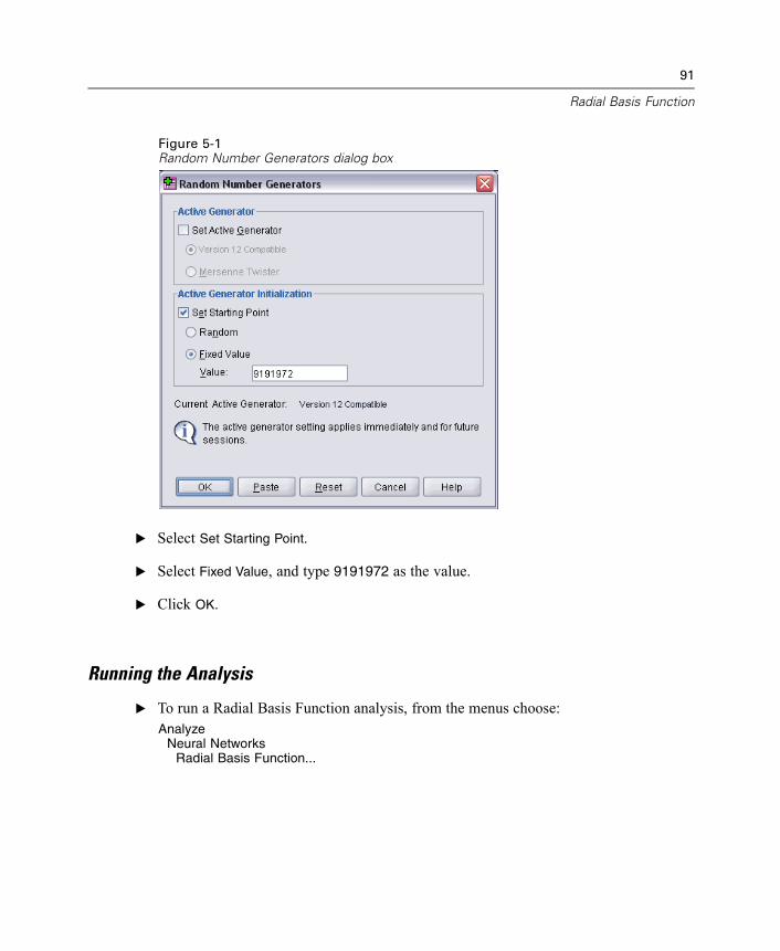
91
Radial Basis Function
Figure 5-1Random Number Generators dialog box
E Select Set Starting Point.
E Select Fixed Value, and type 9191972 as the value.
E Click OK.
Running the Analysis
E To run a Radial Basis Function analysis, from the menus choose:Analyze
Neural NetworksRadial Basis Function...
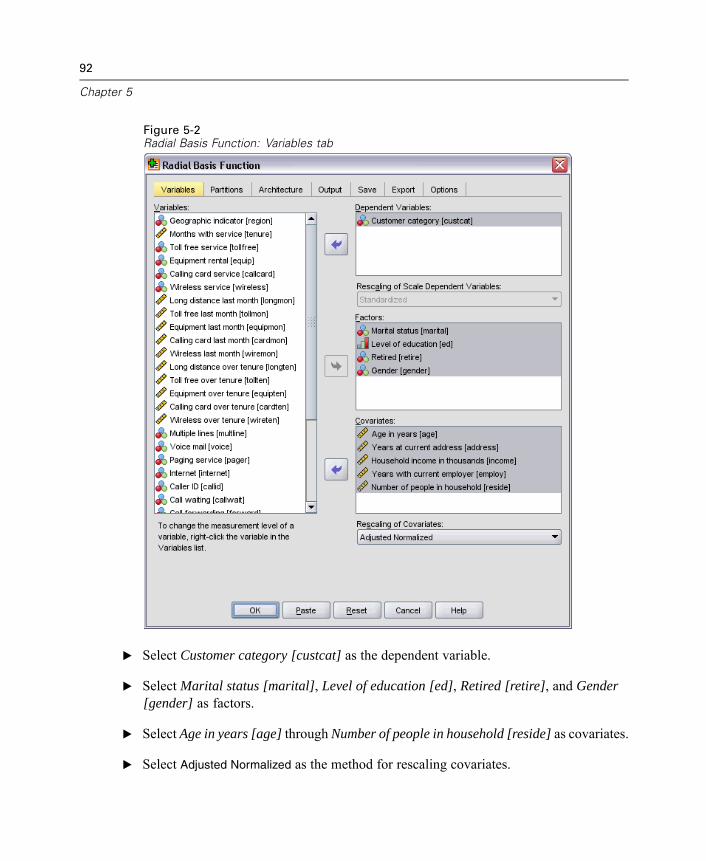
92
Chapter 5
Figure 5-2Radial Basis Function: Variables tab
E Select Customer category [custcat] as the dependent variable.
E Select Marital status [marital], Level of education [ed], Retired [retire], and Gender[gender] as factors.
E Select Age in years [age] through Number of people in household [reside] as covariates.
E Select Adjusted Normalized as the method for rescaling covariates.
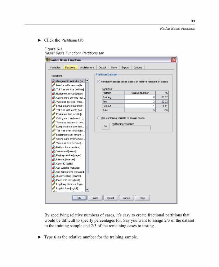
93
Radial Basis Function
E Click the Partitions tab.
Figure 5-3Radial Basis Function: Partitions tab
By specifying relative numbers of cases, it’s easy to create fractional partitions thatwould be difficult to specify percentages for. Say you want to assign 2/3 of the datasetto the training sample and 2/3 of the remaining cases to testing.
E Type 6 as the relative number for the training sample.
94
Chapter 5
E Type 2 as the relative number for the testing sample.
E Type 1 as the relative number for the holdout sample.
A total of 9 relative cases have been specified. 6/9 = 2/3, or about 66.67%, are assignedto the training sample; 2/9, or about 22.22%, are assigned to testing; 1/9, or about11.11% are assigned to the holdout sample.
E Click the Output tab.
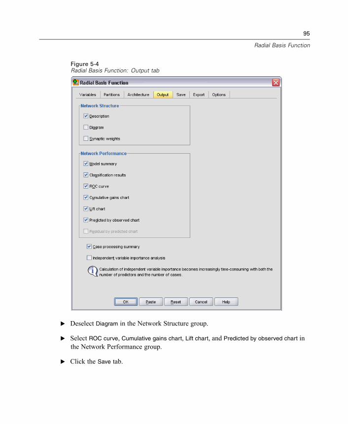
95
Radial Basis Function
Figure 5-4Radial Basis Function: Output tab
E Deselect Diagram in the Network Structure group.
E Select ROC curve, Cumulative gains chart, Lift chart, and Predicted by observed chart inthe Network Performance group.
E Click the Save tab.
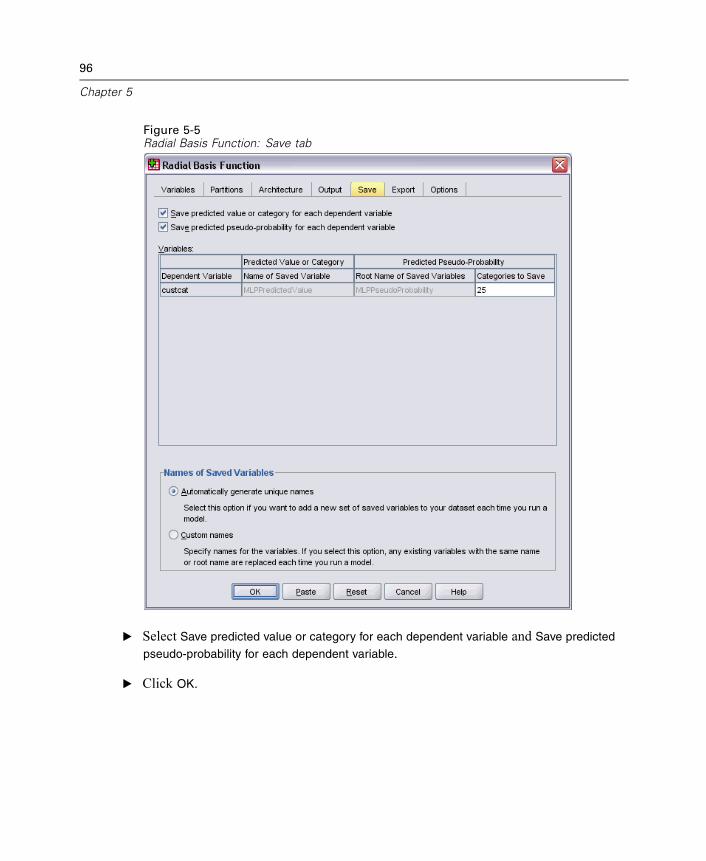
96
Chapter 5
Figure 5-5Radial Basis Function: Save tab
E Select Save predicted value or category for each dependent variable and Save predicted
pseudo-probability for each dependent variable.
E Click OK.
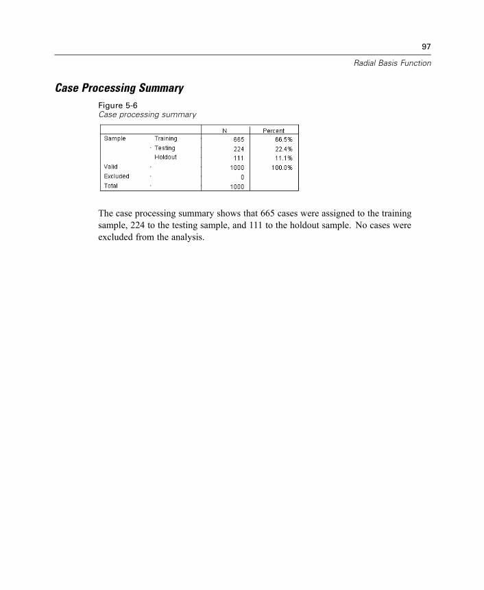
97
Radial Basis Function
Case Processing SummaryFigure 5-6Case processing summary
The case processing summary shows that 665 cases were assigned to the trainingsample, 224 to the testing sample, and 111 to the holdout sample. No cases wereexcluded from the analysis.
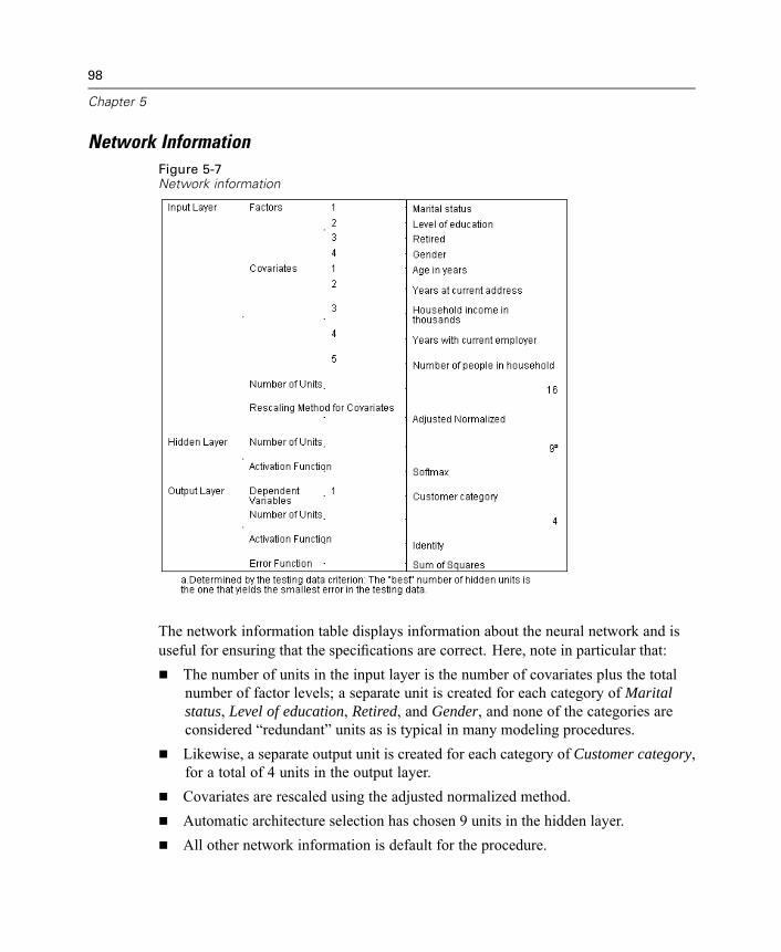
98
Chapter 5
Network InformationFigure 5-7Network information
The network information table displays information about the neural network and isuseful for ensuring that the specifications are correct. Here, note in particular that:
The number of units in the input layer is the number of covariates plus the totalnumber of factor levels; a separate unit is created for each category of Maritalstatus, Level of education, Retired, and Gender, and none of the categories areconsidered “redundant” units as is typical in many modeling procedures.Likewise, a separate output unit is created for each category of Customer category,for a total of 4 units in the output layer.Covariates are rescaled using the adjusted normalized method.Automatic architecture selection has chosen 9 units in the hidden layer.All other network information is default for the procedure.

99
Radial Basis Function
Model SummaryFigure 5-8Model summary
The model summary displays information about the results of training, testing, andapplying the final network to the holdout sample.
Sum of squares error is displayed because that is always used for RBF networks.This is the error function that the network tries to minimize during training andtesting.The percentage of incorrect predictions is taken from the classification table andwill be discussed further in that topic.
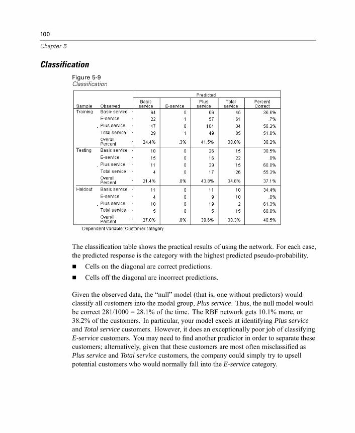
100
Chapter 5
ClassificationFigure 5-9Classification
The classification table shows the practical results of using the network. For each case,the predicted response is the category with the highest predicted pseudo-probability.
Cells on the diagonal are correct predictions.Cells off the diagonal are incorrect predictions.
Given the observed data, the “null” model (that is, one without predictors) wouldclassify all customers into the modal group, Plus service. Thus, the null model wouldbe correct 281/1000 = 28.1% of the time. The RBF network gets 10.1% more, or38.2% of the customers. In particular, your model excels at identifying Plus serviceand Total service customers. However, it does an exceptionally poor job of classifyingE-service customers. You may need to find another predictor in order to separate thesecustomers; alternatively, given that these customers are most often misclassified asPlus service and Total service customers, the company could simply try to upsellpotential customers who would normally fall into the E-service category.
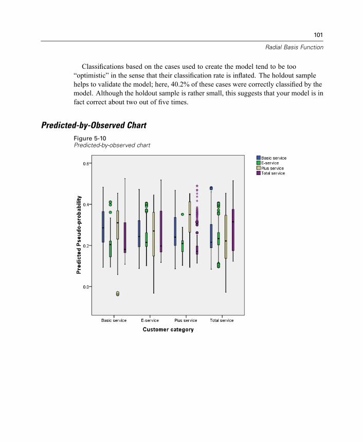
101
Radial Basis Function
Classifications based on the cases used to create the model tend to be too“optimistic” in the sense that their classification rate is inflated. The holdout samplehelps to validate the model; here, 40.2% of these cases were correctly classified by themodel. Although the holdout sample is rather small, this suggests that your model is infact correct about two out of five times.
Predicted-by-Observed ChartFigure 5-10Predicted-by-observed chart
102
Chapter 5
For categorical dependent variables, the predicted-by-observed chart displays clusteredboxplots of predicted pseudo-probabilities for the combined training and testingsamples. The x axis corresponds to the observed response categories, and the legendcorresponds to predicted categories. Thus:
The leftmost boxplot shows, for cases that have observed category Basic service,the predicted pseudo-probability of category Basic service.The next boxplot to the right shows, for cases that have observed category Basicservice, the predicted pseudo-probability of category E-service.The third boxplot shows, for cases that have observed category Basic service,the predicted pseudo-probability of category Plus service. Remember fromthe classification table that roughly as many Basic service customers weremisclassified as Plus service as correctly classified as Basic service; thus, thisboxplot is roughly equivalent to the leftmost.The fourth boxplot shows, for cases that have observed category Basic service, thepredicted pseudo-probability of category Total service
Since there are more than two categories in the target variable, the first four boxplotsare not symmetrical about the horizontal line at 0.5 nor in any other way. As a result,interpreting this plot for targets with more than two categories can be difficult becauseit is impossible to determine, from looking at a portion of cases in one boxplot, thecorresponding location of those cases in another boxplot.

103
Radial Basis Function
ROC CurveFigure 5-11ROC curve
An ROC curve gives you a visual display of the sensitivity by specificity for allpossible classification cutoffs. The chart shown here displays four curves, one for eachcategory of the target variable.Note that this chart is based on the combined training and testing samples. To
produce an ROC chart for the holdout sample, split the file on the partition variableand run the ROC Curve procedure on the predicted pseudo-probabilities.
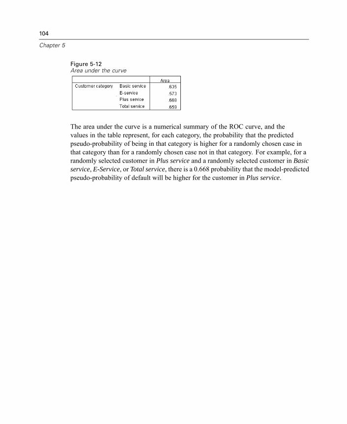
104
Chapter 5
Figure 5-12Area under the curve
The area under the curve is a numerical summary of the ROC curve, and thevalues in the table represent, for each category, the probability that the predictedpseudo-probability of being in that category is higher for a randomly chosen case inthat category than for a randomly chosen case not in that category. For example, for arandomly selected customer in Plus service and a randomly selected customer in Basicservice, E-Service, or Total service, there is a 0.668 probability that the model-predictedpseudo-probability of default will be higher for the customer in Plus service.
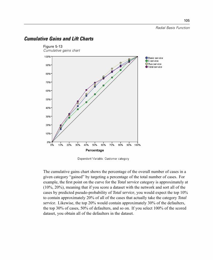
105
Radial Basis Function
Cumulative Gains and Lift ChartsFigure 5-13Cumulative gains chart
The cumulative gains chart shows the percentage of the overall number of cases in agiven category “gained” by targeting a percentage of the total number of cases. Forexample, the first point on the curve for the Total service category is approximately at(10%, 20%), meaning that if you score a dataset with the network and sort all of thecases by predicted pseudo-probability of Total service, you would expect the top 10%to contain approximately 20% of all of the cases that actually take the category Totalservice. Likewise, the top 20% would contain approximately 30% of the defaulters,the top 30% of cases, 50% of defaulters, and so on. If you select 100% of the scoreddataset, you obtain all of the defaulters in the dataset.

106
Chapter 5
The diagonal line is the “baseline” curve; if you select 10% of the cases from thescored dataset at random, you would expect to “gain” approximately 10% of allof the cases that actually take any given category. The farther above the baseline acurve lies, the greater the gain.
Figure 5-14Lift chart
The lift chart is derived from the cumulative gains chart; the values on the y axiscorrespond to the ratio of the cumulative gain for each curve to the baseline. Thus, thelift at 10% for the category Total service is approximately 20%/10% = 2.0. It providesanother way of looking at the information in the cumulative gains chart.
Note: The cumulative gains and lift charts are based on the combined training andtesting samples.

107
Radial Basis Function
Recommended Readings
See the following texts for more information on Radial Basis Function:
Bishop, C. M. 1995. Neural Networks for Pattern Recognition, 3rd ed. Oxford:Oxford University Press.
Fine, T. L. 1999. Feedforward Neural Network Methodology, 3rd ed. New York:Springer-Verlag.
Haykin, S. 1998. Neural Networks: A Comprehensive Foundation, 2nd ed. New York:Macmillan College Publishing.
Ripley, B. D. 1996. Pattern Recognition and Neural Networks. Cambridge:Cambridge University Press.
Tao, K. K. 1993. A closer look at the radial basis function (RBF) networks. In:Conference Record of the Twenty-Seventh Asilomar Conference on Signals, Systems,and Computers, A. Singh, ed. Los Alamitos, Calif.: IEEE Comput. Soc. Press,401–405.
Uykan, Z., C. Guzelis, M. E. Celebi, and H. N. Koivo. 2000. Analysis of input-outputclustering for determining centers of RBFN. IEEE Transactions on Neural Networks,11, 851–858.
Appendix
ASample Files
The sample files installed with the product can be found in the Samples subdirectory ofthe installation directory. There is a separate folder within the Samples subdirectory foreach of the following languages: English, French, German, Italian, Japanese, Korean,Polish, Russian, Simplified Chinese, Spanish, and Traditional Chinese.
Not all sample files are available in all languages. If a sample file is not available in alanguage, that language folder contains an English version of the sample file.
Descriptions
Following are brief descriptions of the sample files used in various examplesthroughout the documentation.
accidents.sav. This is a hypothetical data file that concerns an insurance companythat is studying age and gender risk factors for automobile accidents in a givenregion. Each case corresponds to a cross-classification of age category and gender.adl.sav. This is a hypothetical data file that concerns efforts to determine thebenefits of a proposed type of therapy for stroke patients. Physicians randomlyassigned female stroke patients to one of two groups. The first received thestandard physical therapy, and the second received an additional emotionaltherapy. Three months following the treatments, each patient’s abilities to performcommon activities of daily life were scored as ordinal variables.advert.sav. This is a hypothetical data file that concerns a retailer’s efforts toexamine the relationship between money spent on advertising and the resultingsales. To this end, they have collected past sales figures and the associatedadvertising costs..
108
109
Sample Files
aflatoxin.sav. This is a hypothetical data file that concerns the testing of corn cropsfor aflatoxin, a poison whose concentration varies widely between and within cropyields. A grain processor has received 16 samples from each of 8 crop yields andmeasured the alfatoxin levels in parts per billion (PPB).aflatoxin20.sav. This data file contains the aflatoxin measurements from each of the16 samples from yields 4 and 8 from the aflatoxin.sav data file.anorectic.sav. While working toward a standardized symptomatology ofanorectic/bulimic behavior, researchers (Van der Ham, Meulman, Van Strien, andVan Engeland, 1997) made a study of 55 adolescents with known eating disorders.Each patient was seen four times over four years, for a total of 220 observations.At each observation, the patients were scored for each of 16 symptoms. Symptomscores are missing for patient 71 at time 2, patient 76 at time 2, and patient 47 attime 3, leaving 217 valid observations.autoaccidents.sav. This is a hypothetical data file that concerns the efforts of aninsurance analyst to model the number of automobile accidents per driver whilealso accounting for driver age and gender. Each case represents a separate driverand records the driver’s gender, age in years, and number of automobile accidentsin the last five years.band.sav. This data file contains hypothetical weekly sales figures of music CDsfor a band. Data for three possible predictor variables are also included.bankloan.sav. This is a hypothetical data file that concerns a bank’s efforts to reducethe rate of loan defaults. The file contains financial and demographic informationon 850 past and prospective customers. The first 700 cases are customers whowere previously given loans. The last 150 cases are prospective customers thatthe bank needs to classify as good or bad credit risks.bankloan_binning.sav. This is a hypothetical data file containing financial anddemographic information on 5,000 past customers.behavior.sav. In a classic example (Price and Bouffard, 1974), 52 students wereasked to rate the combinations of 15 situations and 15 behaviors on a 10-pointscale ranging from 0=“extremely appropriate” to 9=“extremely inappropriate.”Averaged over individuals, the values are taken as dissimilarities.behavior_ini.sav. This data file contains an initial configuration for atwo-dimensional solution for behavior.sav.
110
Appendix A
brakes.sav. This is a hypothetical data file that concerns quality control at a factorythat produces disc brakes for high-performance automobiles. The data file containsdiameter measurements of 16 discs from each of 8 production machines. Thetarget diameter for the brakes is 322 millimeters.breakfast.sav. In a classic study (Green and Rao, 1972), 21 Wharton School MBAstudents and their spouses were asked to rank 15 breakfast items in order ofpreference with 1=“most preferred” to 15=“least preferred.” Their preferenceswere recorded under six different scenarios, from “Overall preference” to “Snack,with beverage only.”breakfast-overall.sav. This data file contains the breakfast item preferences for thefirst scenario, “Overall preference,” only.broadband_1.sav. This is a hypothetical data file containing the number ofsubscribers, by region, to a national broadband service. The data file containsmonthly subscriber numbers for 85 regions over a four-year period.broadband_2.sav. This data file is identical to broadband_1.sav but contains datafor three additional months.car_insurance_claims.sav. A dataset presented and analyzed elsewhere (McCullaghand Nelder, 1989) concerns damage claims for cars. The average claim amountcan be modeled as having a gamma distribution, using an inverse link functionto relate the mean of the dependent variable to a linear combination of thepolicyholder age, vehicle type, and vehicle age. The number of claims filed canbe used as a scaling weight.car_sales.sav. This data file contains hypothetical sales estimates, list prices,and physical specifications for various makes and models of vehicles. The listprices and physical specifications were obtained alternately from edmunds.comand manufacturer sites.carpet.sav. In a popular example (Green and Wind, 1973), a company interested inmarketing a new carpet cleaner wants to examine the influence of five factors onconsumer preference—package design, brand name, price, a Good Housekeepingseal, and a money-back guarantee. There are three factor levels for packagedesign, each one differing in the location of the applicator brush; three brandnames (K2R, Glory, and Bissell); three price levels; and two levels (either no oryes) for each of the last two factors. Ten consumers rank 22 profiles defined bythese factors. The variable Preference contains the rank of the average rankingsfor each profile. Low rankings correspond to high preference. This variablereflects an overall measure of preference for each profile.
111
Sample Files
carpet_prefs.sav. This data file is based on the same example as described forcarpet.sav, but it contains the actual rankings collected from each of the 10consumers. The consumers were asked to rank the 22 product profiles from themost to the least preferred. The variables PREF1 through PREF22 contain theidentifiers of the associated profiles, as defined in carpet_plan.sav.catalog.sav. This data file contains hypothetical monthly sales figures for threeproducts sold by a catalog company. Data for five possible predictor variablesare also included.catalog_seasfac.sav. This data file is the same as catalog.sav except for theaddition of a set of seasonal factors calculated from the Seasonal Decompositionprocedure along with the accompanying date variables.cellular.sav. This is a hypothetical data file that concerns a cellular phonecompany’s efforts to reduce churn. Churn propensity scores are applied toaccounts, ranging from 0 to 100. Accounts scoring 50 or above may be looking tochange providers.ceramics.sav. This is a hypothetical data file that concerns a manufacturer’s effortsto determine whether a new premium alloy has a greater heat resistance than astandard alloy. Each case represents a separate test of one of the alloys; the heat atwhich the bearing failed is recorded.cereal.sav. This is a hypothetical data file that concerns a poll of 880 people abouttheir breakfast preferences, also noting their age, gender, marital status, andwhether or not they have an active lifestyle (based on whether they exercise atleast twice a week). Each case represents a separate respondent.clothing_defects.sav. This is a hypothetical data file that concerns the qualitycontrol process at a clothing factory. From each lot produced at the factory, theinspectors take a sample of clothes and count the number of clothes that areunacceptable.coffee.sav. This data file pertains to perceived images of six iced-coffee brands(Kennedy, Riquier, and Sharp, 1996) . For each of 23 iced-coffee image attributes,people selected all brands that were described by the attribute. The six brands aredenoted AA, BB, CC, DD, EE, and FF to preserve confidentiality.contacts.sav. This is a hypothetical data file that concerns the contact lists for agroup of corporate computer sales representatives. Each contact is categorizedby the department of the company in which they work and their company ranks.Also recorded are the amount of the last sale made, the time since the last sale,and the size of the contact’s company.
112
Appendix A
creditpromo.sav. This is a hypothetical data file that concerns a department store’sefforts to evaluate the effectiveness of a recent credit card promotion. To thisend, 500 cardholders were randomly selected. Half received an ad promoting areduced interest rate on purchases made over the next three months. Half receiveda standard seasonal ad.customer_dbase.sav. This is a hypothetical data file that concerns a company’sefforts to use the information in its data warehouse to make special offers tocustomers who are most likely to reply. A subset of the customer base was selectedat random and given the special offers, and their responses were recorded.customer_information.sav. A hypothetical data file containing customer mailinginformation, such as name and address.customers_model.sav. This file contains hypothetical data on individuals targetedby a marketing campaign. These data include demographic information, asummary of purchasing history, and whether or not each individual responded tothe campaign. Each case represents a separate individual.customers_new.sav. This file contains hypothetical data on individuals who arepotential candidates for a marketing campaign. These data include demographicinformation and a summary of purchasing history for each individual. Each caserepresents a separate individual.debate.sav. This is a hypothetical data file that concerns paired responses to asurvey from attendees of a political debate before and after the debate. Each casecorresponds to a separate respondent.debate_aggregate.sav. This is a hypothetical data file that aggregates the responsesin debate.sav. Each case corresponds to a cross-classification of preference beforeand after the debate.demo.sav. This is a hypothetical data file that concerns a purchased customerdatabase, for the purpose of mailing monthly offers. Whether or not the customerresponded to the offer is recorded, along with various demographic information.demo_cs_1.sav. This is a hypothetical data file that concerns the first step ofa company’s efforts to compile a database of survey information. Each casecorresponds to a different city, and the region, province, district, and cityidentification are recorded.demo_cs_2.sav. This is a hypothetical data file that concerns the second stepof a company’s efforts to compile a database of survey information. Each casecorresponds to a different household unit from cities selected in the first step, and

113
Sample Files
the region, province, district, city, subdivision, and unit identification are recorded.The sampling information from the first two stages of the design is also included.demo_cs.sav. This is a hypothetical data file that contains survey informationcollected using a complex sampling design. Each case corresponds to a differenthousehold unit, and various demographic and sampling information is recorded.dietstudy.sav. This hypothetical data file contains the results of a study of the“Stillman diet” (Rickman, Mitchell, Dingman, and Dalen, 1974). Each casecorresponds to a separate subject and records his or her pre- and post-diet weightsin pounds and triglyceride levels in mg/100 ml.dischargedata.sav. This is a data file concerning Seasonal Patterns of WinnipegHospital Use, (Menec , Roos, Nowicki, MacWilliam, Finlayson , and Black, 1999)from the Manitoba Centre for Health Policy.dvdplayer.sav. This is a hypothetical data file that concerns the development of anew DVD player. Using a prototype, the marketing team has collected focusgroup data. Each case corresponds to a separate surveyed user and records somedemographic information about them and their responses to questions about theprototype.flying.sav. This data file contains the flying mileages between 10 American cities.german_credit.sav. This data file is taken from the “German credit” dataset inthe Repository of Machine Learning Databases (Blake and Merz, 1998) at theUniversity of California, Irvine.grocery_1month.sav. This hypothetical data file is the grocery_coupons.sav data filewith the weekly purchases “rolled-up” so that each case corresponds to a separatecustomer. Some of the variables that changed weekly disappear as a result, andthe amount spent recorded is now the sum of the amounts spent during the fourweeks of the study.grocery_coupons.sav. This is a hypothetical data file that contains survey datacollected by a grocery store chain interested in the purchasing habits of theircustomers. Each customer is followed for four weeks, and each case correspondsto a separate customer-week and records information about where and how thecustomer shops, including how much was spent on groceries during that week.guttman.sav. Bell (Bell, 1961) presented a table to illustrate possible social groups.Guttman (Guttman, 1968) used a portion of this table, in which five variablesdescribing such things as social interaction, feelings of belonging to a group,physical proximity of members, and formality of the relationship were crossedwith seven theoretical social groups, including crowds (for example, people at a
114
Appendix A
football game), audiences (for example, people at a theater or classroom lecture),public (for example, newspaper or television audiences), mobs (like a crowd butwith much more intense interaction), primary groups (intimate), secondary groups(voluntary), and the modern community (loose confederation resulting from closephysical proximity and a need for specialized services).healthplans.sav. This is a hypothetical data file that concerns an insurance group’sefforts to evaluate four different health care plans for small employers. Twelveemployers are recruited to rank the plans by how much they would prefer tooffer them to their employees. Each case corresponds to a separate employerand records the reactions to each plan.health_funding.sav. This is a hypothetical data file that contains data on health carefunding (amount per 100 population), disease rates (rate per 10,000 population),and visits to health care providers (rate per 10,000 population). Each caserepresents a different city.hivassay.sav. This is a hypothetical data file that concerns the efforts of apharmaceutical lab to develop a rapid assay for detecting HIV infection. Theresults of the assay are eight deepening shades of red, with deeper shades indicatinggreater likelihood of infection. A laboratory trial was conducted on 2,000 bloodsamples, half of which were infected with HIV and half of which were clean.hourlywagedata.sav. This is a hypothetical data file that concerns the hourly wagesof nurses from office and hospital positions and with varying levels of experience.insure.sav. This is a hypothetical data file that concerns an insurance company thatis studying the risk factors that indicate whether a client will have to make a claimon a 10-year term life insurance contract. Each case in the data file represents apair of contracts, one of which recorded a claim and the other didn’t, matchedon age and gender.judges.sav. This is a hypothetical data file that concerns the scores given by trainedjudges (plus one enthusiast) to 300 gymnastics performances. Each row representsa separate performance; the judges viewed the same performances.kinship_dat.sav. Rosenberg and Kim (Rosenberg and Kim, 1975) set out toanalyze 15 kinship terms (aunt, brother, cousin, daughter, father, granddaughter,grandfather, grandmother, grandson, mother, nephew, niece, sister, son, uncle).They asked four groups of college students (two female, two male) to sort theseterms on the basis of similarities. Two groups (one female, one male) were askedto sort twice, with the second sorting based on a different criterion from the firstsort. Thus, a total of six “sources” were obtained. Each source corresponds to a
115
Sample Files
proximity matrix, whose cells are equal to the number of people in a sourceminus the number of times the objects were partitioned together in that source.kinship_ini.sav. This data file contains an initial configuration for athree-dimensional solution for kinship_dat.sav.kinship_var.sav. This data file contains independent variables gender, gener(ation),and degree (of separation) that can be used to interpret the dimensions of a solutionfor kinship_dat.sav. Specifically, they can be used to restrict the space of thesolution to a linear combination of these variables.mailresponse.sav. This is a hypothetical data file that concerns the efforts of aclothing manufacturer to determine whether using first class postage for directmailings results in faster responses than bulk mail. Order-takers record how manyweeks after the mailing each order is taken.marketvalues.sav. This data file concerns home sales in a new housing developmentin Algonquin, Ill., during the years from 1999–2000. These sales are a matterof public record.mutualfund.sav. This data file concerns stock market information for various techstocks listed on the S&P 500. Each case corresponds to a separate company.nhis2000_subset.sav. The National Health Interview Survey (NHIS) is a large,population-based survey of the U.S. civilian population. Interviews arecarried out face-to-face in a nationally representative sample of households.Demographic information and observations about health behaviors and statusare obtained for members of each household. This data file contains a subsetof information from the 2000 survey. National Center for Health Statistics.National Health Interview Survey, 2000. Public-use data file and documentation.ftp://ftp.cdc.gov/pub/Health_Statistics/NCHS/Datasets/NHIS/2000/. Accessed2003.ozone.sav. The data include 330 observations on six meteorological variables forpredicting ozone concentration from the remaining variables. Previous researchers(Breiman and Friedman, 1985), (Hastie and Tibshirani, 1990), among others foundnonlinearities among these variables, which hinder standard regression approaches.pain_medication.sav. This hypothetical data file contains the results of a clinicaltrial for anti-inflammatory medication for treating chronic arthritic pain. Ofparticular interest is the time it takes for the drug to take effect and how itcompares to an existing medication.
116
Appendix A
patient_los.sav. This hypothetical data file contains the treatment records ofpatients who were admitted to the hospital for suspected myocardial infarction(MI, or “heart attack”). Each case corresponds to a separate patient and recordsmany variables related to their hospital stay.patlos_sample.sav. This hypothetical data file contains the treatment records of asample of patients who received thrombolytics during treatment for myocardialinfarction (MI, or “heart attack”). Each case corresponds to a separate patient andrecords many variables related to their hospital stay.polishing.sav. This is the “Nambeware Polishing Times” data file from the Data andStory Library. It concerns the efforts of a metal tableware manufacturer (NambeMills, Santa Fe, N. M.) to plan its production schedule. Each case represents adifferent item in the product line. The diameter, polishing time, price, and producttype are recorded for each item.poll_cs.sav. This is a hypothetical data file that concerns pollsters’ efforts todetermine the level of public support for a bill before the legislature. The casescorrespond to registered voters. Each case records the county, township, andneighborhood in which the voter lives.poll_cs_sample.sav. This hypothetical data file contains a sample of the voterslisted in poll_cs.sav. The sample was taken according to the design specified inthe poll.csplan plan file, and this data file records the inclusion probabilities andsample weights. Note, however, that because the sampling plan makes use ofa probability-proportional-to-size (PPS) method, there is also a file containingthe joint selection probabilities (poll_jointprob.sav). The additional variablescorresponding to voter demographics and their opinion on the proposed bill werecollected and added the data file after the sample as taken.property_assess.sav. This is a hypothetical data file that concerns a countyassessor’s efforts to keep property value assessments up to date on limitedresources. The cases correspond to properties sold in the county in the past year.Each case in the data file records the township in which the property lies, theassessor who last visited the property, the time since that assessment, the valuationmade at that time, and the sale value of the property.property_assess_cs.sav. This is a hypothetical data file that concerns a stateassessor’s efforts to keep property value assessments up to date on limitedresources. The cases correspond to properties in the state. Each case in the datafile records the county, township, and neighborhood in which the property lies, thetime since the last assessment, and the valuation made at that time.
117
Sample Files
property_assess_cs_sample.sav. This hypothetical data file contains a sample ofthe properties listed in property_assess_cs.sav. The sample was taken accordingto the design specified in the property_assess.csplan plan file, and this data filerecords the inclusion probabilities and sample weights. The additional variableCurrent value was collected and added to the data file after the sample was taken.recidivism.sav. This is a hypothetical data file that concerns a government lawenforcement agency’s efforts to understand recidivism rates in their area ofjurisdiction. Each case corresponds to a previous offender and records theirdemographic information, some details of their first crime, and then the time untiltheir second arrest, if it occurred within two years of the first arrest.recidivism_cs_sample.sav. This is a hypothetical data file that concerns agovernment law enforcement agency’s efforts to understand recidivism ratesin their area of jurisdiction. Each case corresponds to a previous offender,released from their first arrest during the month of June, 2003, and recordstheir demographic information, some details of their first crime, and the dataof their second arrest, if it occurred by the end of June, 2006. Offenders wereselected from sampled departments according to the sampling plan specified inrecidivism_cs.csplan; because it makes use of a probability-proportional-to-size(PPS) method, there is also a file containing the joint selection probabilities(recidivism_cs_jointprob.sav).rfm_transactions.sav. A hypothetical data file containing purchase transactiondata, including date of purchase, item(s) purchased, and monetary amount ofeach transaction.salesperformance.sav. This is a hypothetical data file that concerns the evaluationof two new sales training courses. Sixty employees, divided into three groups, allreceive standard training. In addition, group 2 gets technical training; group 3,a hands-on tutorial. Each employee was tested at the end of the training courseand their score recorded. Each case in the data file represents a separate traineeand records the group to which they were assigned and the score they receivedon the exam.satisf.sav. This is a hypothetical data file that concerns a satisfaction surveyconducted by a retail company at 4 store locations. 582 customers were surveyedin all, and each case represents the responses from a single customer.screws.sav. This data file contains information on the characteristics of screws,bolts, nuts, and tacks (Hartigan, 1975).
118
Appendix A
shampoo_ph.sav. This is a hypothetical data file that concerns the quality control ata factory for hair products. At regular time intervals, six separate output batchesare measured and their pH recorded. The target range is 4.5–5.5.ships.sav. A dataset presented and analyzed elsewhere (McCullagh et al., 1989)that concerns damage to cargo ships caused by waves. The incident counts can bemodeled as occurring at a Poisson rate given the ship type, construction period, andservice period. The aggregate months of service for each cell of the table formedby the cross-classification of factors provides values for the exposure to risk.site.sav. This is a hypothetical data file that concerns a company’s efforts to choosenew sites for their expanding business. They have hired two consultants toseparately evaluate the sites, who, in addition to an extended report, summarizedeach site as a “good,” “fair,” or “poor” prospect.siteratings.sav. This is a hypothetical data file that concerns the beta testing of ane-commerce firm’s new Web site. Each case represents a separate beta tester, whoscored the usability of the site on a scale from 0–20.smokers.sav. This data file is abstracted from the 1998 National Household Surveyof Drug Abuse and is a probability sample of American households. Thus, thefirst step in an analysis of this data file should be to weight the data to reflectpopulation trends.smoking.sav. This is a hypothetical table introduced by Greenacre (Greenacre,1984). The table of interest is formed by the crosstabulation of smoking behaviorby job category. The variable Staff Group contains the job categories Sr Managers,Jr Managers, Sr Employees, Jr Employees, and Secretaries, plus the categoryNational Average, which can be used as supplementary to an analysis. Thevariable Smoking contains the behaviors None, Light, Medium, and Heavy, plusthe categories No Alcohol and Alcohol, which can be used as supplementary to ananalysis.storebrand.sav. This is a hypothetical data file that concerns a grocery storemanager’s efforts to increase sales of the store brand detergent relative to otherbrands. She puts together an in-store promotion and talks with customers atcheck-out. Each case represents a separate customer.stores.sav. This data file contains hypothetical monthly market share data fortwo competing grocery stores. Each case represents the market share data for agiven month.stroke_clean.sav. This hypothetical data file contains the state of a medicaldatabase after it has been cleaned using procedures in the Data Preparation option.
119
Sample Files
stroke_invalid.sav. This hypothetical data file contains the initial state of a medicaldatabase and contains several data entry errors.stroke_survival. This hypothetical data file concerns survival times for patientsexiting a rehabilitation program post-ischemic stroke face a number of challenges.Post-stroke, the occurrence of myocardial infarction, ischemic stroke, orhemorrhagic stroke is noted and the time of the event recorded. The sample isleft-truncated because it only includes patients who survived through the end ofthe rehabilitation program administered post-stroke.stroke_valid.sav. This hypothetical data file contains the state of a medical databaseafter the values have been checked using the Validate Data procedure. It stillcontains potentially anomalous cases.survey_sample.sav. This hypothetical data file contains survey data, includingdemographic data and various attitude measures.tastetest.sav. This is a hypothetical data file that concerns the effect of mulch coloron the taste of crops. Strawberries grown in red, blue, and black mulch were ratedby taste-testers on an ordinal scale of 1 to 5 (far below to far above average). Eachcase represents a separate taste-tester.telco.sav. This is a hypothetical data file that concerns a telecommunicationscompany’s efforts to reduce churn in their customer base. Each case correspondsto a separate customer and records various demographic and service usageinformation.telco_extra.sav. This data file is similar to the telco.sav data file, but the “tenure”and log-transformed customer spending variables have been removed and replacedby standardized log-transformed customer spending variables.telco_missing.sav. This data file is a subset of the telco.sav data file, but some ofthe demographic data values have been replaced with missing values.testmarket.sav. This hypothetical data file concerns a fast food chain’s plans toadd a new item to its menu. There are three possible campaigns for promotingthe new product, so the new item is introduced at locations in several randomlyselected markets. A different promotion is used at each location, and the weeklysales of the new item are recorded for the first four weeks. Each case correspondsto a separate location-week.testmarket_1month.sav. This hypothetical data file is the testmarket.sav data filewith the weekly sales “rolled-up” so that each case corresponds to a separatelocation. Some of the variables that changed weekly disappear as a result, and thesales recorded is now the sum of the sales during the four weeks of the study.
120
Appendix A
tree_car.sav. This is a hypothetical data file containing demographic and vehiclepurchase price data.tree_credit.sav. This is a hypothetical data file containing demographic and bankloan history data.tree_missing_data.sav This is a hypothetical data file containing demographic andbank loan history data with a large number of missing values.tree_score_car.sav. This is a hypothetical data file containing demographic andvehicle purchase price data.tree_textdata.sav. A simple data file with only two variables intended primarilyto show the default state of variables prior to assignment of measurement leveland value labels.tv-survey.sav. This is a hypothetical data file that concerns a survey conducted by aTV studio that is considering whether to extend the run of a successful program.906 respondents were asked whether they would watch the program under variousconditions. Each row represents a separate respondent; each column is a separatecondition.ulcer_recurrence.sav. This file contains partial information from a study designedto compare the efficacy of two therapies for preventing the recurrence of ulcers. Itprovides a good example of interval-censored data and has been presented andanalyzed elsewhere (Collett, 2003).ulcer_recurrence_recoded.sav. This file reorganizes the information inulcer_recurrence.sav to allow you model the event probability for each intervalof the study rather than simply the end-of-study event probability. It has beenpresented and analyzed elsewhere (Collett et al., 2003).verd1985.sav. This data file concerns a survey (Verdegaal, 1985). The responsesof 15 subjects to 8 variables were recorded. The variables of interest are dividedinto three sets. Set 1 includes age and marital, set 2 includes pet and news, and set3 includes music and live. Pet is scaled as multiple nominal and age is scaled asordinal; all of the other variables are scaled as single nominal.virus.sav. This is a hypothetical data file that concerns the efforts of an Internetservice provider (ISP) to determine the effects of a virus on its networks. Theyhave tracked the (approximate) percentage of infected e-mail traffic on its networksover time, from the moment of discovery until the threat was contained.

121
Sample Files
waittimes.sav. This is a hypothetical data file that concerns customer waiting timesfor service at three different branches of a local bank. Each case corresponds toa separate customer and records the time spent waiting and the branch at whichthey were conducting their business.webusability.sav. This is a hypothetical data file that concerns usability testing ofa new e-store. Each case corresponds to one of five usability testers and recordswhether or not the tester succeeded at each of six separate tasks.wheeze_steubenville.sav. This is a subset from a longitudinal study of the healtheffects of air pollution on children (Ware, Dockery, Spiro III, Speizer, and FerrisJr., 1984). The data contain repeated binary measures of the wheezing statusfor children from Steubenville, Ohio, at ages 7, 8, 9 and 10 years, along with afixed recording of whether or not the mother was a smoker during the first yearof the study.workprog.sav. This is a hypothetical data file that concerns a government worksprogram that tries to place disadvantaged people into better jobs. A sample ofpotential program participants were followed, some of whom were randomlyselected for enrollment in the program, while others were not. Each case representsa separate program participant.

Bibliography
Bell, E. H. 1961. Social foundations of human behavior: Introduction to the study ofsociology. New York: Harper & Row.
Bishop, C. M. 1995. Neural Networks for Pattern Recognition, 3rd ed. Oxford:Oxford University Press.
Blake, C. L., and C. J. Merz. 1998. "UCI Repository of machine learning databases."Available at http://www.ics.uci.edu/~mlearn/MLRepository.html.
Breiman, L., and J. H. Friedman. 1985. Estimating optimal transformations formultiple regression and correlation. Journal of the American Statistical Association,80, 580–598.
Collett, D. 2003. Modelling survival data in medical research, 2 ed. Boca Raton:Chapman & Hall/CRC.
Fine, T. L. 1999. Feedforward Neural Network Methodology, 3rd ed. New York:Springer-Verlag.
Green, P. E., and V. Rao. 1972. Applied multidimensional scaling. Hinsdale, Ill.:Dryden Press.
Green, P. E., and Y. Wind. 1973. Multiattribute decisions in marketing: A measurementapproach. Hinsdale, Ill.: Dryden Press.
Greenacre, M. J. 1984. Theory and applications of correspondence analysis. London:Academic Press.
Guttman, L. 1968. A general nonmetric technique for finding the smallest coordinatespace for configurations of points. Psychometrika, 33, 469–506.
Hartigan, J. A. 1975. Clustering algorithms. New York: John Wiley and Sons.
Hastie, T., and R. Tibshirani. 1990. Generalized additive models. London: Chapmanand Hall.
Haykin, S. 1998. Neural Networks: A Comprehensive Foundation, 2nd ed. New York:Macmillan College Publishing.
Kennedy, R., C. Riquier, and B. Sharp. 1996. Practical applications of correspondenceanalysis to categorical data in market research. Journal of Targeting, Measurement,and Analysis for Marketing, 5, 56–70.
122

123
Bibliography
McCullagh, P., and J. A. Nelder. 1989. Generalized Linear Models, 2nd ed. London:Chapman & Hall.
Menec , V., N. Roos, D. Nowicki, L. MacWilliam, G. Finlayson , and C. Black. 1999.Seasonal Patterns of Winnipeg Hospital Use. : Manitoba Centre for Health Policy.
Price, R. H., and D. L. Bouffard. 1974. Behavioral appropriateness and situationalconstraints as dimensions of social behavior. Journal of Personality and SocialPsychology, 30, 579–586.
Rickman, R., N. Mitchell, J. Dingman, and J. E. Dalen. 1974. Changes in serumcholesterol during the Stillman Diet. Journal of the American Medical Association,228, 54–58.
Ripley, B. D. 1996. Pattern Recognition and Neural Networks. Cambridge:Cambridge University Press.
Rosenberg, S., and M. P. Kim. 1975. The method of sorting as a data-gatheringprocedure in multivariate research. Multivariate Behavioral Research, 10, 489–502.
Tao, K. K. 1993. A closer look at the radial basis function (RBF) networks. In:Conference Record of the Twenty-Seventh Asilomar Conference on Signals, Systems,and Computers, A. Singh, ed. Los Alamitos, Calif.: IEEE Comput. Soc. Press,401–405.
Uykan, Z., C. Guzelis, M. E. Celebi, and H. N. Koivo. 2000. Analysis of input-outputclustering for determining centers of RBFN. IEEE Transactions on Neural Networks,11, 851–858.
Van der Ham, T., J. J. Meulman, D. C. Van Strien, and H. Van Engeland. 1997.Empirically based subgrouping of eating disorders in adolescents: A longitudinalperspective. British Journal of Psychiatry, 170, 363–368.
Verdegaal, R. 1985. Meer sets analyse voor kwalitatieve gegevens (in Dutch). Leiden:Department of Data Theory, University of Leiden.
Ware, J. H., D. W. Dockery, A. Spiro III, F. E. Speizer, and B. G. Ferris Jr.. 1984.Passive smoking, gas cooking, and respiratory health of children living in six cities.American Review of Respiratory Diseases, 129, 366–374.

Index
activation functionin Multilayer Perceptron, 13in Radial Basis Function, 35
architectureneural networks, 3
batch trainingin Multilayer Perceptron, 16
case processing summaryin Multilayer Perceptron, 52, 57, 80in Radial Basis Function, 97
classificationin Multilayer Perceptron, 54, 60in Radial Basis Function, 100
cumulative gains chartin Multilayer Perceptron, 65in Radial Basis Function, 105
gains chartin Multilayer Perceptron, 19in Radial Basis Function, 37
hidden layerin Multilayer Perceptron, 13in Radial Basis Function, 35
holdout samplein Multilayer Perceptron, 11in Radial Basis Function, 33
importancein Multilayer Perceptron, 68, 88
lift chartin Multilayer Perceptron, 19, 65in Radial Basis Function, 37, 105
mini-batch trainingin Multilayer Perceptron, 16
missing valuesin Multilayer Perceptron, 25
Multilayer Perceptron, 5, 45case processing summary, 52, 57, 80classification, 54, 60cumulative gains chart, 65independent variable importance, 68, 88lift chart, 65model export, 24model summary, 53, 59, 82network architecture, 13network information, 52, 58, 81options, 25output, 19overtraining, 54partition variable, 46partitions, 11predicted-by-observed chart, 63, 84residual-by-predicted chart, 86ROC curve, 61save variables to active dataset, 22training, 16warnings, 80
network architecturein Multilayer Perceptron, 13in Radial Basis Function, 35
network diagramin Multilayer Perceptron, 19in Radial Basis Function, 37
network informationin Multilayer Perceptron, 52, 58, 81in Radial Basis Function, 98
network trainingin Multilayer Perceptron, 16
neural networksarchitecture, 3definition, 1
124

125
Index
online trainingin Multilayer Perceptron, 16
output layerin Multilayer Perceptron, 13in Radial Basis Function, 35
overtrainingin Multilayer Perceptron, 54
partition variablein Multilayer Perceptron, 46
predicted-by-observed chartin Radial Basis Function, 101
Radial Basis Function, 28, 90case processing summary, 97classification, 100cumulative gains chart, 105lift chart, 105model export, 42model summary, 99network architecture, 35network information, 98options, 43output, 37partitions, 33predicted-by-observed chart, 101ROC curve, 103save variables to active dataset, 40something, 90
ROC curvein Multilayer Perceptron, 19, 61in Radial Basis Function, 37, 103
sample fileslocation, 108
somethingin Radial Basis Function, 90
stopping rulesin Multilayer Perceptron, 25
testing samplein Multilayer Perceptron, 11in Radial Basis Function, 33
training samplein Multilayer Perceptron, 11in Radial Basis Function, 33
warningsin Multilayer Perceptron, 80