spss statistics brief guide 17.0
TRANSCRIPT
5/11/2018 SPSS Statistics Brief Guide 17.0 - slidepdf.com
http://slidepdf.com/reader/full/spss-statistics-brief-guide-170-55a2339b08a28 1/224
i
SPSSStatistics17.0Brief Guide
5/11/2018 SPSS Statistics Brief Guide 17.0 - slidepdf.com
http://slidepdf.com/reader/full/spss-statistics-brief-guide-170-55a2339b08a28 2/224
For more information about SPSS Inc. software products, please visit our Web site at http://www.spss.com or con
SPSS Inc.
233 South Wacker Drive, 11th Floor
Chicago, IL 60606-6412
Tel: (312) 651-3000
Fax: (312) 651-3668
SPSS is a registered trademark and the other product names are the trademarks of SPSS Inc. for its proprietary co
software. No material describing such software may be produced or distributed without the written permission o
owners of the trademark and license rights in the software and the copyrights in the published materials.
The SOFTWARE and documentation are provided with RESTRICTED RIGHTS. Use, duplication, or disclosure
the Government is subject to restrictions as set forth in subdivision (c) (1) (ii) of The Rights in Technical Data an
Computer Software clause at 52.227-7013. Contractor/manufacturer is SPSS Inc., 233 South Wacker Drive, 11th
Floor, Chicago, IL 60606-6412.
Patent No. 7,023,453
General notice: Other product names mentioned herein are used for identification purposes only and may be trade
of their respective companies.
Windows is a registered trademark of Microsoft Corporation.
Apple, Mac, and the Mac logo are trademarks of Apple Computer, Inc., registered in the U.S. and other countries
This product uses WinWrap Basic, Copyright 1993-2007, Polar Engineering and Consulting, http://www.winwrap
Printed in the United States of America.
No part of this publication may be reproduced, stored in a retrieval system, or transmitted, in any form or by any
electronic, mechanical, photocopying, recording, or otherwise, without the prior written permission of the publish
ISBN-13: 978-1-56827-401-0
ISBN-10: 1-56827-401-7
1 2 3 4 5 6 7 8 9 0 11 10 09 08
5/11/2018 SPSS Statistics Brief Guide 17.0 - slidepdf.com
http://slidepdf.com/reader/full/spss-statistics-brief-guide-170-55a2339b08a28 3/224
Prefac
The SPSS Statistics 17.0 Brief Guide provides a set of tutorials designed to acquain
you with the various components of SPSS Statistics. This guide is intended for use
with all operating system versions of the software, including: Windows, Macintosh
and Linux. You can work through the tutorials in sequence or turn to the topics for
which you need additional information. You can use this guide as a supplement to t
online tutorial that is included with the SPSS Statistics Base 17.0 system or ignore t
online tutorial and start with the tutorials found here.
SPSS Statistics 17.0
SPSS Statistics 17.0 is a comprehensive system for analyzing data. SPSS Statistics
can take data from almost any type of file and use them to generate tabulated report
charts, and plots of distributions and trends, descriptive statistics, and complex
statistical analyses.
SPSS Statistics makes statistical analysis more accessible for the beginner and m
convenient for the experienced user. Simple menus and dialog box selections make
possible to perform complex analyses without typing a single line of command synt
The Data Editor offers a simple and ef ficient spreadsheet-like facility for entering
data and browsing the working data file.
Internet Resources
The SPSS Inc. Web site (http://www.spss.com) offers answers to frequently asked
questions and provides access to data files and other useful information.
In addition, the SPSS USENET discussion group (not sponsored by SPSS Inc.) i
open to anyone interested . The USENET address is comp.soft-sys.stat.spss.You can also subscribe to an e-mail message list that is gatewayed to the USENE
group. To subscribe, send an e-mail message to [email protected] . The text
the e-mail message should be: subscribe SPSSX-L firstname lastname. You can th
post messages to the list by sending an e-mail message to [email protected]
iii
5/11/2018 SPSS Statistics Brief Guide 17.0 - slidepdf.com
http://slidepdf.com/reader/full/spss-statistics-brief-guide-170-55a2339b08a28 4/224
Additional Publications The Statistical Procedures Companion, by Marija Norušis, has been published b
Prentice Hall. It contains overviews of the procedures in SPSS Statistics Base, plus
Logistic Regression and General Linear Models. The Advanced Statistical Procedu
Companion has also been published by Prentice Hall. It includes overviews of the procedures in the Advanced and Regression modules.
SPSS Statistics Options
The following options are available as add-on enhancements to the full (not Studen
Version) SPSS Statistics Base system:
Regression provides techniques for analyzing data that do not fit traditional linear
statistical models. It includes procedures for probit analysis, logistic regression, wei
estimation, two-stage least-squares regression, and general nonlinear regression.
Advanced Statistics focuses on techniques often used in sophisticated experimental a
biomedical research. It includes procedures for general linear models (GLM), linea
mixed models, variance components analysis, loglinear analysis, ordinal regression
actuarial life tables, Kaplan-Meier survival analysis, and basic and extended Cox
regression.
Custom Tables creates a variety of presentation-quality tabular reports, including
complex stub-and-banner tables and displays of multiple response data.
Forecasting performs comprehensive forecasting and time series analyses with multicurve-fitting models, smoothing models, and methods for estimating autoregressive
functions.
Categories performs optimal scaling procedures, including correspondence analysis
Conjoint provides a realistic way to measure how individual product attributes affec
consumer and citizen preferences. With Conjoint, you can easily measure the trade-
effect of each product attribute in the context of a set of product attributes—as
consumers do when making purchasing decisions.
Exact Tests calculates exact p values for statistical tests when small or very unevenl
distributed samples could make the usual tests inaccurate. This option is available oon Windows operating systems.
Missing Values describes patterns of missing data, estimates means and other statist
and imputes values for missing observations.
iv
5/11/2018 SPSS Statistics Brief Guide 17.0 - slidepdf.com
http://slidepdf.com/reader/full/spss-statistics-brief-guide-170-55a2339b08a28 5/224
Complex Samples allows survey, market, health, and public opinion researchers, as w
as social scientists who use sample survey methodology, to incorporate their compl
sample designs into data analysis.
Decision Trees creates a tree-based classification model. It classifies cases into grouor predicts values of a dependent (target) variable based on values of independent
(predictor) variables. The procedure provides validation tools for exploratory and
confirmatory classification analysis.
Data Preparation provides a quick visual snapshot of your data. It provides the abili
to apply validation rules that identify invalid data values. You can create rules that fl
out-of-range values, missing values, or blank values. You can also save variables th
record individual rule violations and the total number of rule violations per case. A
limited set of predefined rules that you can copy or modify is provided.
Neural Networks can be used to make business decisions by forecasting demand for product as a function of price and other variables, or by categorizing customers bas
on buying habits and demographic characteristics. Neural networks are non-linear d
modeling tools. They can be used to model complex relationships between inputs
and outputs or to find patterns in data.
EZ RFM performs RFM (receny, frequency, monetary) analysis on transaction data fi
and customer data files.
Amos™ (analysis of moment structures) uses structural equation modeling to confir
and explain conceptual models that involve attitudes, perceptions, and other factors
that drive behavior.
Training Seminars
SPSS Inc. provides both public and onsite training seminars for SPSS Statistics. A
seminars feature hands-on workshops. seminars will be offered in major U.S. and
European cities on a regular basis. For more information on these seminars, contac
your local of fice, listed on the SPSS Inc. Web site at http://www.spss.com/worldwid
Technical Support
Technical Support services are available to maintenance customers of SPSS Statisti
(Student Version customers should read the special section on technical support for
the Student Version. For more information, see Technical Support for Students on p
vii.) Customers may contact Technical Support for assistance in using products or f
v
5/11/2018 SPSS Statistics Brief Guide 17.0 - slidepdf.com
http://slidepdf.com/reader/full/spss-statistics-brief-guide-170-55a2339b08a28 6/224
installation help for one of the supported hardware environments. To reach Technic
Support, see the web site at http://www.spss.com, or contact your local of fice, listed
the SPSS Inc. Web site at http://www.spss.com/worldwide . Be prepared to identify
yourself, your organization, and the serial number of your system.
SPSS Statistics 17.0 for Windows Student Version
The SPSS Statistics 17.0 for Windows Student Version is a limited but still powerfu
version of the SPSS Statistics Base 17.0 system.
Capability
The Student Version contains all of the important data analysis tools contained in th
full SPSS Statistics Base system, including: Spreadsheet-like Data Editor for entering, modifying, and viewing data files.
Statistical procedures, including t tests, analysis of variance, and crosstabulation
Interactive graphics that allow you to change or add chart elements and variable
dynamically; the changes appear as soon as they are specified.
Standard high-resolution graphics for an extensive array of analytical and
presentation charts and tables.
Limitations
Created for classroom instruction, the Student Version is limited to use by students a
instructors for educational purposes only. The Student Version does not contain all
the functions of the SPSS Statistics Base 17.0 system. The following limitations ap
to the SPSS Statistics 17.0 for Windows Student Version:
Data files cannot contain more than 50 variables.
Data files cannot contain more than 1,500 cases. SPSS Statistics add-on modul
(such as Regression or Advanced Statistics) cannot be used with the Student
Version.
vi
5/11/2018 SPSS Statistics Brief Guide 17.0 - slidepdf.com
http://slidepdf.com/reader/full/spss-statistics-brief-guide-170-55a2339b08a28 7/224
SPSS Statistics command syntax is not available to the user. This means that it
not possible to repeat an analysis by saving a series of commands in a syntax o
“job” file, as can be done in the full version of SPSS Statistics.
Scripting and automation are not available to the user. This means that you canncreate scripts that automate tasks that you repeat often, as can be done in the fu
version of SPSS Statistics.
Technical Support for Students
Students should obtain technical support from their instructors or from local suppor
staff identified by their instructors. Technical support for the SPSS Statistics 17.0
Student Version is provided only to instructors using the system for classroom
instruction.
Before seeking assistance from your instructor, please write down the informatiodescribed below. Without this information, your instructor may be unable to assist y
The type of computer you are using, as well as the amount of RAM and free dis
space you have.
The operating system of your computer.
A clear description of what happened and what you were doing when the proble
occurred. If possible, please try to reproduce the problem with one of the samp
data files provided with the program.
The exact wording of any error or warning messages that appeared on your scre
How you tried to solve the problem on your own.
Technical Support for Instructors
Instructors using the Student Version for classroom instruction may contact Technic
Support for assistance. In the United States and Canada, call Technical Support at
(312) 651-3410, or send an e-mail to [email protected]. Please include your name
title, and academic institution.
Instructors outside of the United States and Canada should contact your local of fi
listed on the web site at http://www.spss.com/worldwide .
vii
5/11/2018 SPSS Statistics Brief Guide 17.0 - slidepdf.com
http://slidepdf.com/reader/full/spss-statistics-brief-guide-170-55a2339b08a28 8/224
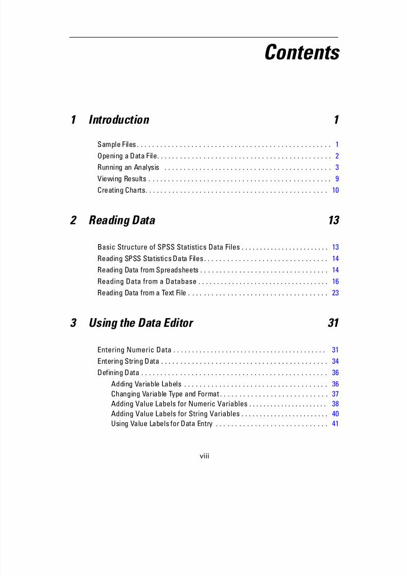
Contents
1 Introduction 1
Sample Files . . . . . . . . . . . . . . . . . . . . . . . . . . . . . . . . . . . . . . . . . . . . . . . . . . 1
Opening a Data File. . . . . . . . . . . . . . . . . . . . . . . . . . . . . . . . . . . . . . . . . . . . . 2
Running an Analysis . . . . . . . . . . . . . . . . . . . . . . . . . . . . . . . . . . . . . . . . . . . 3
Viewing Results . . . . . . . . . . . . . . . . . . . . . . . . . . . . . . . . . . . . . . . . . . . . . . . 9
Creating Charts. . . . . . . . . . . . . . . . . . . . . . . . . . . . . . . . . . . . . . . . . . . . . . . 10
2 Reading Data 13
Basic Structure of SPSS Statistics Data Files . . . . . . . . . . . . . . . . . . . . . . . . 13
Reading SPSS Statistics Data Files . . . . . . . . . . . . . . . . . . . . . . . . . . . . . . . . 14
Reading Data from Spreadsheets . . . . . . . . . . . . . . . . . . . . . . . . . . . . . . . . . 14
Reading Data from a Database . . . . . . . . . . . . . . . . . . . . . . . . . . . . . . . . . . . 16
Reading Data from a Text File . . . . . . . . . . . . . . . . . . . . . . . . . . . . . . . . . . . . 23
3 Using the Data Editor 31
Entering Numeric Data . . . . . . . . . . . . . . . . . . . . . . . . . . . . . . . . . . . . . . . . . 31
Entering String Data . . . . . . . . . . . . . . . . . . . . . . . . . . . . . . . . . . . . . . . . . . . 34
Defining Data . . . . . . . . . . . . . . . . . . . . . . . . . . . . . . . . . . . . . . . . . . . . . . . . 36
Adding Variable Labels . . . . . . . . . . . . . . . . . . . . . . . . . . . . . . . . . . . . . 36
Changing Variable Type and Format . . . . . . . . . . . . . . . . . . . . . . . . . . . . 37
Adding Value Labels for Numeric Variables . . . . . . . . . . . . . . . . . . . . . . 38
Adding Value Labels for String Variables . . . . . . . . . . . . . . . . . . . . . . . . 40
Using Value Labels for Data Entry . . . . . . . . . . . . . . . . . . . . . . . . . . . . . 41
viii
5/11/2018 SPSS Statistics Brief Guide 17.0 - slidepdf.com
http://slidepdf.com/reader/full/spss-statistics-brief-guide-170-55a2339b08a28 9/224
Handling Missing Data. . . . . . . . . . . . . . . . . . . . . . . . . . . . . . . . . . . . . . 42
Missing Values for a Numeric Variable. . . . . . . . . . . . . . . . . . . . . . . . . . 43Missing Values for a String Variable. . . . . . . . . . . . . . . . . . . . . . . . . . . . 45
Copying and Pasting Variable Attributes . . . . . . . . . . . . . . . . . . . . . . . . 46
Defining Variable Properties for Categorical Variables . . . . . . . . . . . . . . 50
4 Working with Multiple Data Sources 57
Basic Handling of Multiple Data Sources . . . . . . . . . . . . . . . . . . . . . . . . . . . 58
Working with Multiple Datasets in Command Syntax. . . . . . . . . . . . . . . . . . . 60
Copying and Pasting Information between Datasets . . . . . . . . . . . . . . . . . . . 60
Renaming Datasets. . . . . . . . . . . . . . . . . . . . . . . . . . . . . . . . . . . . . . . . . . . . 61
Suppressing Multiple Datasets . . . . . . . . . . . . . . . . . . . . . . . . . . . . . . . . . . . 61
5 Examining Summary Statistics for Individual Variables 62
Level of Measurement . . . . . . . . . . . . . . . . . . . . . . . . . . . . . . . . . . . . . . . . . 62Summary Measures for Categorical Data . . . . . . . . . . . . . . . . . . . . . . . . . . . 63
Charts for Categorical Data . . . . . . . . . . . . . . . . . . . . . . . . . . . . . . . . . . 64
Summary Measures for Scale Variables . . . . . . . . . . . . . . . . . . . . . . . . . . . . 66
Histograms for Scale Variables . . . . . . . . . . . . . . . . . . . . . . . . . . . . . . . 69
6 Creating and Edi ting Charts 72
Chart Creation Basics. . . . . . . . . . . . . . . . . . . . . . . . . . . . . . . . . . . . . . . . . . 72Using the Chart Builder Gallery . . . . . . . . . . . . . . . . . . . . . . . . . . . . . . . 73
Defining Variables and Statistics . . . . . . . . . . . . . . . . . . . . . . . . . . . . . . 76
ix
5/11/2018 SPSS Statistics Brief Guide 17.0 - slidepdf.com
http://slidepdf.com/reader/full/spss-statistics-brief-guide-170-55a2339b08a28 10/224
Adding Text . . . . . . . . . . . . . . . . . . . . . . . . . . . . . . . . . . . . . . . . . . . . . . 79
Creating the Chart . . . . . . . . . . . . . . . . . . . . . . . . . . . . . . . . . . . . . . . . . 81Chart Editing Basics . . . . . . . . . . . . . . . . . . . . . . . . . . . . . . . . . . . . . . . . . . . 81
Selecting Chart Elements. . . . . . . . . . . . . . . . . . . . . . . . . . . . . . . . . . . . 82
Using the Properties Window . . . . . . . . . . . . . . . . . . . . . . . . . . . . . . . . 83
Changing Bar Colors . . . . . . . . . . . . . . . . . . . . . . . . . . . . . . . . . . . . . . . 84
Formatting Numbers in Tick Labels . . . . . . . . . . . . . . . . . . . . . . . . . . . . 86
Editing Text . . . . . . . . . . . . . . . . . . . . . . . . . . . . . . . . . . . . . . . . . . . . . . 88
Displaying Data Value Labels. . . . . . . . . . . . . . . . . . . . . . . . . . . . . . . . . 89
Using Templates . . . . . . . . . . . . . . . . . . . . . . . . . . . . . . . . . . . . . . . . . . 90
Defining Chart Options. . . . . . . . . . . . . . . . . . . . . . . . . . . . . . . . . . . . . . 96
7 Working with Output 100
Using the Viewer . . . . . . . . . . . . . . . . . . . . . . . . . . . . . . . . . . . . . . . . . . . . 100
Using the Pivot Table Editor . . . . . . . . . . . . . . . . . . . . . . . . . . . . . . . . . . . . 102
Accessing Output Definitions. . . . . . . . . . . . . . . . . . . . . . . . . . . . . . . . 102
Pivoting Tables . . . . . . . . . . . . . . . . . . . . . . . . . . . . . . . . . . . . . . . . . . 103
Creating and Displaying Layers . . . . . . . . . . . . . . . . . . . . . . . . . . . . . . 106
Editing Tables . . . . . . . . . . . . . . . . . . . . . . . . . . . . . . . . . . . . . . . . . . . 108Hiding Rows and Columns . . . . . . . . . . . . . . . . . . . . . . . . . . . . . . . . . . 109
Changing Data Display Formats . . . . . . . . . . . . . . . . . . . . . . . . . . . . . . 110
TableLooks . . . . . . . . . . . . . . . . . . . . . . . . . . . . . . . . . . . . . . . . . . . . . . . . . 112
Using Predefined Formats . . . . . . . . . . . . . . . . . . . . . . . . . . . . . . . . . . 112
Customizing TableLook Styles . . . . . . . . . . . . . . . . . . . . . . . . . . . . . . . 113
Changing the Default Table Formats. . . . . . . . . . . . . . . . . . . . . . . . . . . 116
Customizing the Initial Display Settings . . . . . . . . . . . . . . . . . . . . . . . . 118
Displaying Variable and Value Labels. . . . . . . . . . . . . . . . . . . . . . . . . . 119
Using Results in Other Applications . . . . . . . . . . . . . . . . . . . . . . . . . . . . . . 122
Pasting Results as Word Tables . . . . . . . . . . . . . . . . . . . . . . . . . . . . . . 122Pasting Results as Text . . . . . . . . . . . . . . . . . . . . . . . . . . . . . . . . . . . . 123
Exporting Results to Microsoft Word, PowerPoint, and Excel Files . . . . 125
x
5/11/2018 SPSS Statistics Brief Guide 17.0 - slidepdf.com
http://slidepdf.com/reader/full/spss-statistics-brief-guide-170-55a2339b08a28 11/224
Exporting Results to PDF . . . . . . . . . . . . . . . . . . . . . . . . . . . . . . . . . . . 134
Exporting Results to HTML. . . . . . . . . . . . . . . . . . . . . . . . . . . . . . . . . . 137
8 Working with Syntax 139
Pasting Syntax . . . . . . . . . . . . . . . . . . . . . . . . . . . . . . . . . . . . . . . . . . . . . . 139
Editing Syntax. . . . . . . . . . . . . . . . . . . . . . . . . . . . . . . . . . . . . . . . . . . . . . . 141
Opening and Running a Syntax File . . . . . . . . . . . . . . . . . . . . . . . . . . . . . . . 143
Understanding the Error Pane. . . . . . . . . . . . . . . . . . . . . . . . . . . . . . . . . . . 144
Using Breakpoints . . . . . . . . . . . . . . . . . . . . . . . . . . . . . . . . . . . . . . . . . . . 145
9 Modifying Data Values 147
Creating a Categorical Variable from a Scale Variable. . . . . . . . . . . . . . . . . 147
Computing New Variables. . . . . . . . . . . . . . . . . . . . . . . . . . . . . . . . . . . . . . 153
Using Functions in Expressions . . . . . . . . . . . . . . . . . . . . . . . . . . . . . . 155
Using Conditional Expressions . . . . . . . . . . . . . . . . . . . . . . . . . . . . . . . 157
Working with Dates and Times . . . . . . . . . . . . . . . . . . . . . . . . . . . . . . . . . . 159Calculating the Length of Time between Two Dates . . . . . . . . . . . . . . . 160
Adding a Duration to a Date. . . . . . . . . . . . . . . . . . . . . . . . . . . . . . . . . 164
10 Sorting and Sel ecting Data 168
Sorting Data . . . . . . . . . . . . . . . . . . . . . . . . . . . . . . . . . . . . . . . . . . . . . . . . 168
Split-File Processing. . . . . . . . . . . . . . . . . . . . . . . . . . . . . . . . . . . . . . . . . . 169
Sorting Cases for Split-File Processing . . . . . . . . . . . . . . . . . . . . . . . . 172Turning Split-File Processing On and Off . . . . . . . . . . . . . . . . . . . . . . . 172
xi
5/11/2018 SPSS Statistics Brief Guide 17.0 - slidepdf.com
http://slidepdf.com/reader/full/spss-statistics-brief-guide-170-55a2339b08a28 12/224
Selecting Subsets of Cases. . . . . . . . . . . . . . . . . . . . . . . . . . . . . . . . . . . . . 173
Selecting Cases Based on Conditional Expressions . . . . . . . . . . . . . . . 174Selecting a Random Sample . . . . . . . . . . . . . . . . . . . . . . . . . . . . . . . . 175
Selecting a Time Range or Case Range . . . . . . . . . . . . . . . . . . . . . . . . 176
Treatment of Unselected Cases . . . . . . . . . . . . . . . . . . . . . . . . . . . . . . 177
Case Selection Status. . . . . . . . . . . . . . . . . . . . . . . . . . . . . . . . . . . . . . . . . 178
11 Additional Statistical Procedures 179
Summarizing Data. . . . . . . . . . . . . . . . . . . . . . . . . . . . . . . . . . . . . . . . . . . . 179
Explore . . . . . . . . . . . . . . . . . . . . . . . . . . . . . . . . . . . . . . . . . . . . . . . . 180
More about Summarizing Data. . . . . . . . . . . . . . . . . . . . . . . . . . . . . . . 181
Comparing Means . . . . . . . . . . . . . . . . . . . . . . . . . . . . . . . . . . . . . . . . . . . 181
Means. . . . . . . . . . . . . . . . . . . . . . . . . . . . . . . . . . . . . . . . . . . . . . . . . 182
Paired-Samples T Test. . . . . . . . . . . . . . . . . . . . . . . . . . . . . . . . . . . . . 183
More about Comparing Means . . . . . . . . . . . . . . . . . . . . . . . . . . . . . . 184
ANOVA Models. . . . . . . . . . . . . . . . . . . . . . . . . . . . . . . . . . . . . . . . . . . . . . 185
Univariate Analysis of Variance . . . . . . . . . . . . . . . . . . . . . . . . . . . . . . 185
Correlating Variables . . . . . . . . . . . . . . . . . . . . . . . . . . . . . . . . . . . . . . . . . 187
Bivariate Correlations . . . . . . . . . . . . . . . . . . . . . . . . . . . . . . . . . . . . . 187Partial Correlations . . . . . . . . . . . . . . . . . . . . . . . . . . . . . . . . . . . . . . . 187
Regression Analysis . . . . . . . . . . . . . . . . . . . . . . . . . . . . . . . . . . . . . . . . . . 188
Linear Regression . . . . . . . . . . . . . . . . . . . . . . . . . . . . . . . . . . . . . . . . 189
Nonparametric Tests . . . . . . . . . . . . . . . . . . . . . . . . . . . . . . . . . . . . . . . . . 190
Chi-Square . . . . . . . . . . . . . . . . . . . . . . . . . . . . . . . . . . . . . . . . . . . . . 190
xii

5/11/2018 SPSS Statistics Brief Guide 17.0 - slidepdf.com
http://slidepdf.com/reader/full/spss-statistics-brief-guide-170-55a2339b08a28 13/224
Appendix
A Sample Files 194
Index 208
xiii

5/11/2018 SPSS Statistics Brief Guide 17.0 - slidepdf.com
http://slidepdf.com/reader/full/spss-statistics-brief-guide-170-55a2339b08a28 14/224
5/11/2018 SPSS Statistics Brief Guide 17.0 - slidepdf.com
http://slidepdf.com/reader/full/spss-statistics-brief-guide-170-55a2339b08a28 15/224
Chapt
1
Introduction
This guide provides a set of tutorials designed to enable you to perform useful analy
on your data. You can work through the tutorials in sequence or turn to the topics fo
which you need additional information.
This chapter will introduce you to the basic features and demonstrate a typical
session. We will retrieve a previously defined SPSS Statistics data file and then
produce a simple statistical summary and a chart.
More detailed instruction about many of the topics touched upon in this chapter
will follow in later chapters. Here, we hope to give you a basic framework for
understanding later tutorials.
Sample Files
Most of the examples that are presented here use the data file demo.sav. This data fi
is a fictitious survey of several thousand people, containing basic demographic and
consumer information.
The sample files installed with the product can be found in the Samples subdirectory
the installation directory. There is a separate folder within the Samples subdirectory
each of the following languages: English, French, German, Italian, Japanese, Korea
Polish, Russian, Simplified Chinese, Spanish, and Traditional Chinese.
Not all sample files are available in all languages. If a sample file is not available in
language, that language folder contains an English version of the sample file.
1
5/11/2018 SPSS Statistics Brief Guide 17.0 - slidepdf.com
http://slidepdf.com/reader/full/spss-statistics-brief-guide-170-55a2339b08a28 16/224
2
Chapter 1
Opening a Data File
To open a data file:
E From the menus choose:
FileOpen
Data...
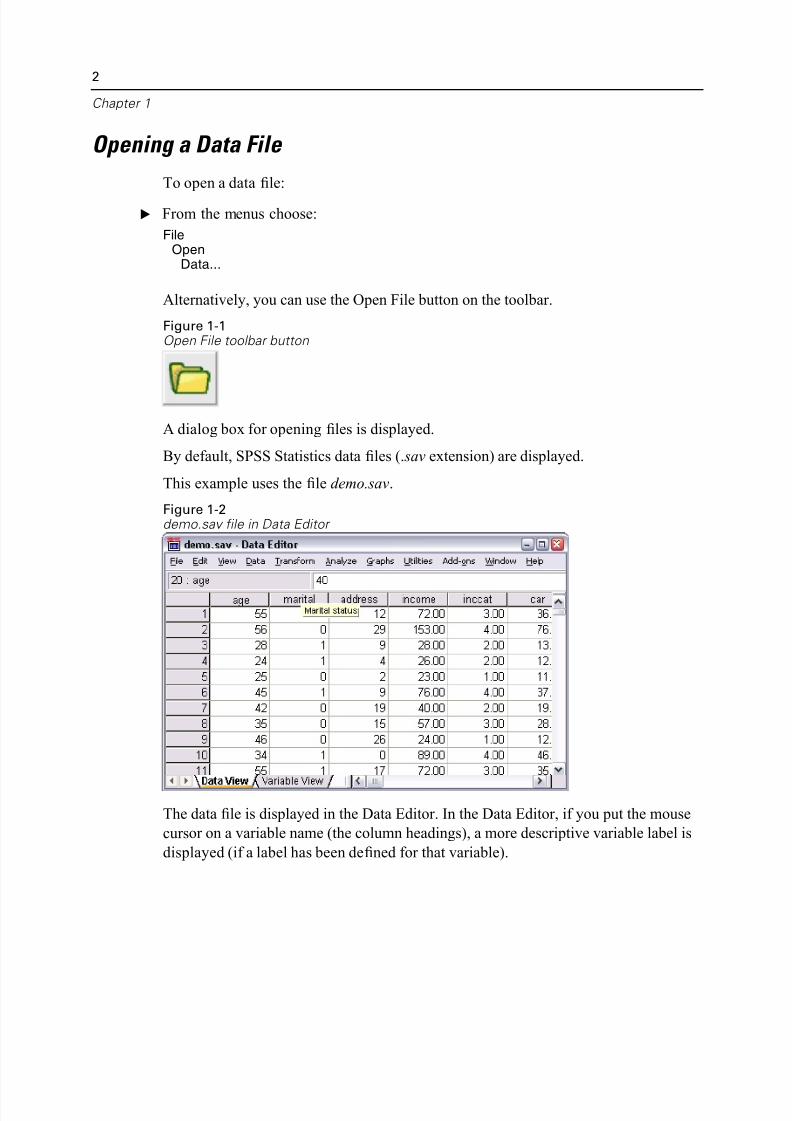
Alternatively, you can use the Open File button on the toolbar.
Figure 1-1Open File toolbar button
A dialog box for opening files is displayed.
By default, SPSS Statistics data files (.sav extension) are displayed.
This example uses the file demo.sav.
Figure 1-2demo.sav file in Data Editor
The data file is displayed in the Data Editor. In the Data Editor, if you put the mous
cursor on a variable name (the column headings), a more descriptive variable label
displayed (if a label has been defined for that variable).
5/11/2018 SPSS Statistics Brief Guide 17.0 - slidepdf.com
http://slidepdf.com/reader/full/spss-statistics-brief-guide-170-55a2339b08a28 17/224
Introduc
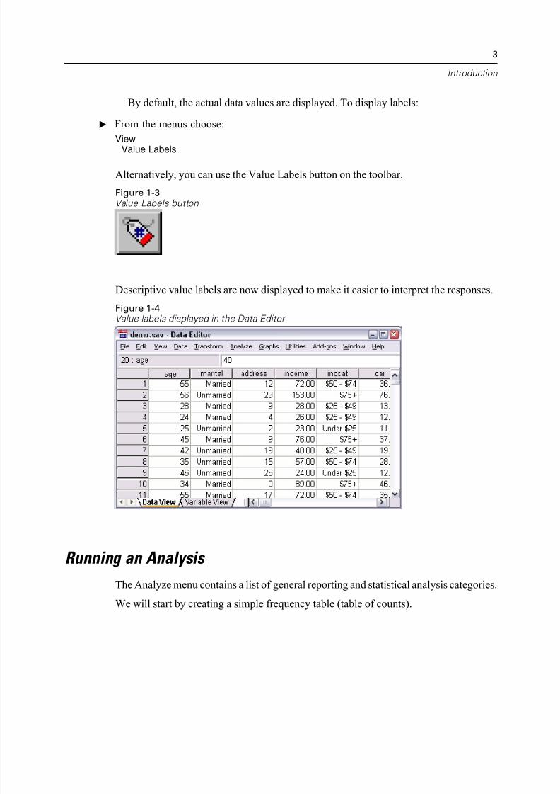
By default, the actual data values are displayed. To display labels:
E From the menus choose:
ViewValue Labels
Alternatively, you can use the Value Labels button on the toolbar.
Figure 1-3Value Labels button
Descriptive value labels are now displayed to make it easier to interpret the respons
Figure 1-4Value labels displayed in the Data Editor
Running an Analysis
The Analyze menu contains a list of general reporting and statistical analysis categor
We will start by creating a simple frequency table (table of counts).
5/11/2018 SPSS Statistics Brief Guide 17.0 - slidepdf.com
http://slidepdf.com/reader/full/spss-statistics-brief-guide-170-55a2339b08a28 18/224
4
Chapter 1
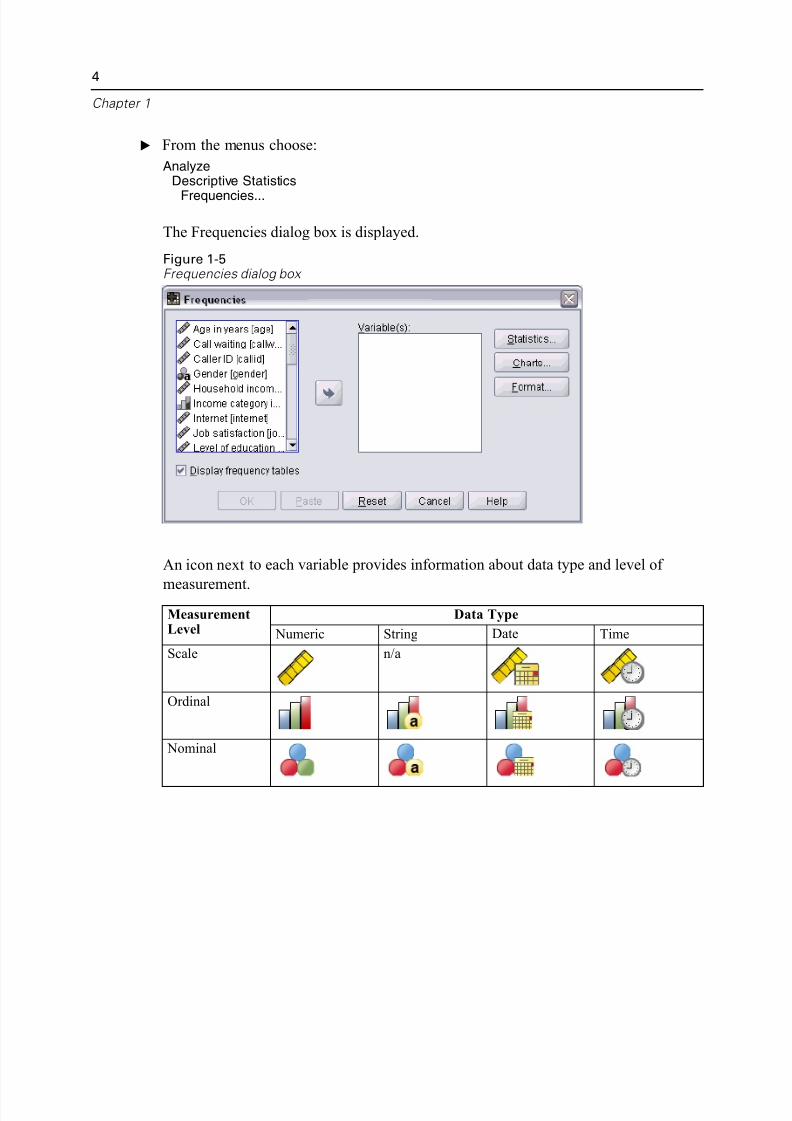
E From the menus choose:
AnalyzeDescriptive Statistics
Frequencies...
The Frequencies dialog box is displayed.
Figure 1-5Frequencies dialog box
An icon next to each variable provides information about data type and level of
measurement.
Data TypeMeasurementLevel Numeric String Date Time
Scale n/a
Ordinal
Nominal
5/11/2018 SPSS Statistics Brief Guide 17.0 - slidepdf.com
http://slidepdf.com/reader/full/spss-statistics-brief-guide-170-55a2339b08a28 19/224
Introduc
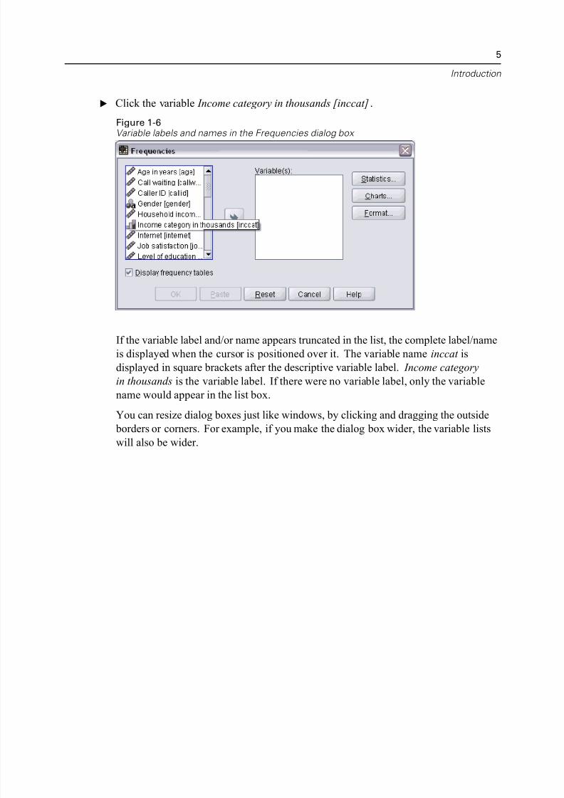
E Click the variable Income category in thousands [inccat].
Figure 1-6
Variable labels and names in the Frequencies dialog box
If the variable label and/or name appears truncated in the list, the complete label/nam
is displayed when the cursor is positioned over it. The variable name inccat is
displayed in square brackets after the descriptive variable label. Income category
in thousands is the variable label. If there were no variable label, only the variable
name would appear in the list box.
You can resize dialog boxes just like windows, by clicking and dragging the outsid borders or corners. For example, if you make the dialog box wider, the variable list
will also be wider.
5/11/2018 SPSS Statistics Brief Guide 17.0 - slidepdf.com
http://slidepdf.com/reader/full/spss-statistics-brief-guide-170-55a2339b08a28 20/224
6
Chapter 1
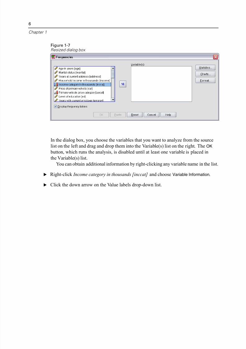
Figure 1-7Resized dialog box
In the dialog box, you choose the variables that you want to analyze from the sourc
list on the left and drag and drop them into the Variable(s) list on the right. The OK
button, which runs the analysis, is disabled until at least one variable is placed in
the Variable(s) list.
You can obtain additional information by right-clicking any variable name in the
E Right-click Income category in thousands [inccat] and choose Variable Information.
E Click the down arrow on the Value labels drop-down list.
5/11/2018 SPSS Statistics Brief Guide 17.0 - slidepdf.com
http://slidepdf.com/reader/full/spss-statistics-brief-guide-170-55a2339b08a28 21/224
Introduc
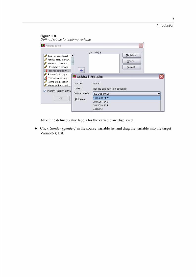
Figure 1-8Defined labels for income variable
All of the defined value labels for the variable are displayed.
E Click Gender [gender] in the source variable list and drag the variable into the targ
Variable(s) list.
5/11/2018 SPSS Statistics Brief Guide 17.0 - slidepdf.com
http://slidepdf.com/reader/full/spss-statistics-brief-guide-170-55a2339b08a28 22/224
8
Chapter 1
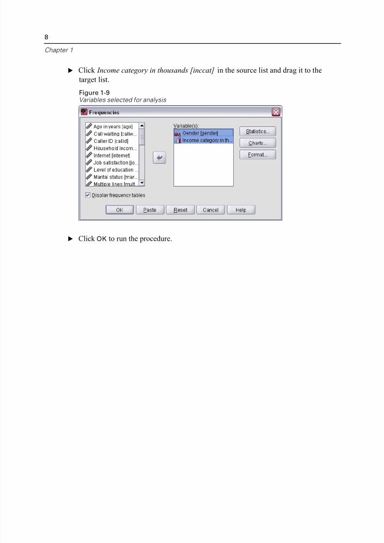
E Click Income category in thousands [inccat] in the source list and drag it to the
target list.
Figure 1-9Variables selected for analysis
E Click OK to run the procedure.
5/11/2018 SPSS Statistics Brief Guide 17.0 - slidepdf.com
http://slidepdf.com/reader/full/spss-statistics-brief-guide-170-55a2339b08a28 23/224
Introduc
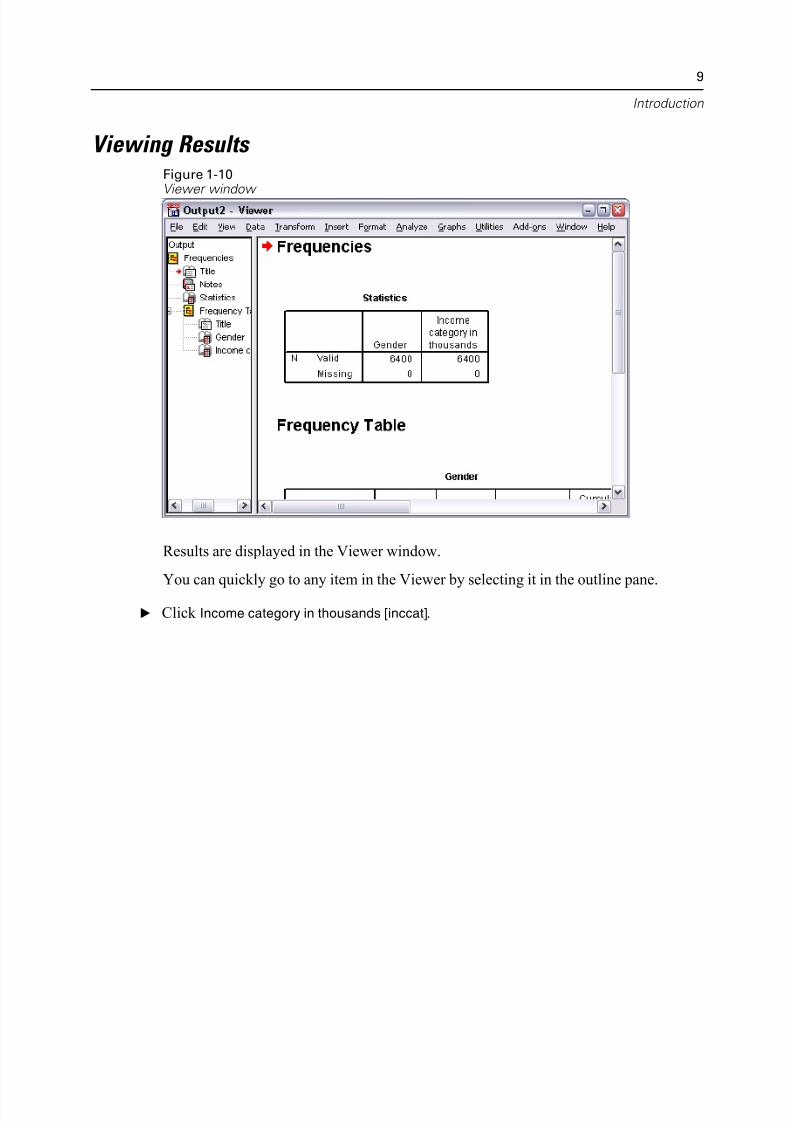
Viewing Results Figure 1-10
Viewer window
Results are displayed in the Viewer window.
You can quickly go to any item in the Viewer by selecting it in the outline pane.
E Click Income category in thousands [inccat].
5/11/2018 SPSS Statistics Brief Guide 17.0 - slidepdf.com
http://slidepdf.com/reader/full/spss-statistics-brief-guide-170-55a2339b08a28 24/224
10
Chapter 1
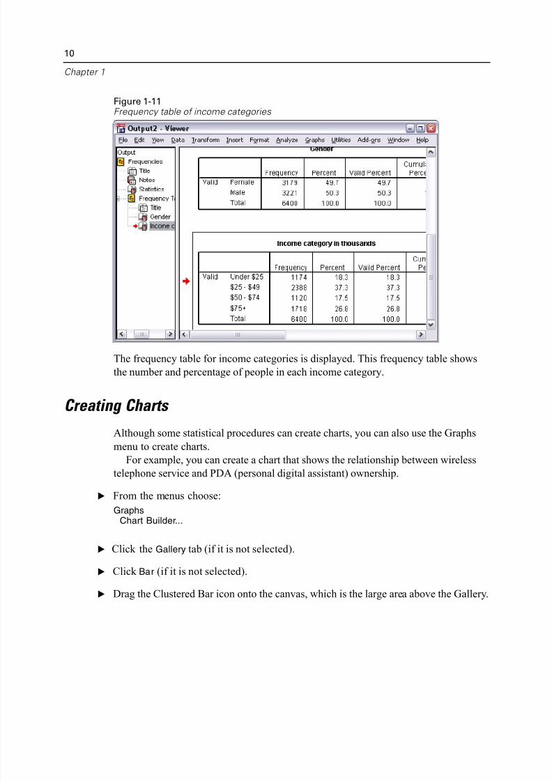
Figure 1-11Frequency table of income categories
The frequency table for income categories is displayed. This frequency table shows
the number and percentage of people in each income category.
Creating Charts Although some statistical procedures can create charts, you can also use the Graphs
menu to create charts.
For example, you can create a chart that shows the relationship between wireless
telephone service and PDA (personal digital assistant) ownership.
E From the menus choose:
GraphsChart Builder...
E Click the Gallery tab (if it is not selected).
E Click Bar (if it is not selected).
E Drag the Clustered Bar icon onto the canvas, which is the large area above the Galle
5/11/2018 SPSS Statistics Brief Guide 17.0 - slidepdf.com
http://slidepdf.com/reader/full/spss-statistics-brief-guide-170-55a2339b08a28 25/224
Introduc
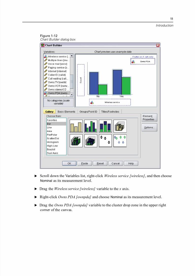
Figure 1-12Chart Builder dialog box
E Scroll down the Variables list, right-click Wireless service [wireless], and then choo
Nominal as its measurement level.
E Drag the Wireless service [wireless] variable to the x axis.
E Right-click Owns PDA [ownpda] and choose Nominal as its measurement level.
E Drag the Owns PDA [ownpda] variable to the cluster drop zone in the upper right
corner of the canvas.
5/11/2018 SPSS Statistics Brief Guide 17.0 - slidepdf.com
http://slidepdf.com/reader/full/spss-statistics-brief-guide-170-55a2339b08a28 26/224
12
Chapter 1
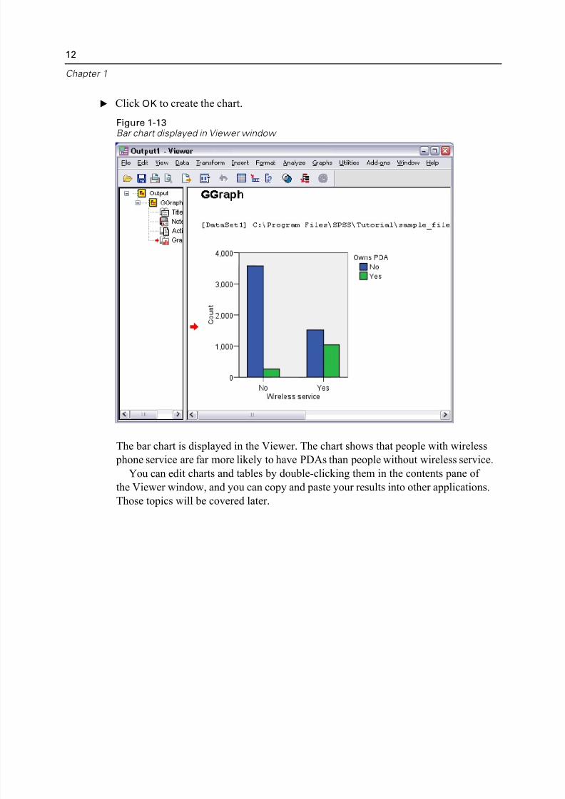
E Click OK to create the chart.
Figure 1-13Bar chart displayed in Viewer window
The bar chart is displayed in the Viewer. The chart shows that people with wireless
phone service are far more likely to have PDAs than people without wireless servic
You can edit charts and tables by double-clicking them in the contents pane of
the Viewer window, and you can copy and paste your results into other applications
Those topics will be covered later.
5/11/2018 SPSS Statistics Brief Guide 17.0 - slidepdf.com
http://slidepdf.com/reader/full/spss-statistics-brief-guide-170-55a2339b08a28 27/224
Chapt
2
Reading Data
Data can be entered directly, or it can be imported from a number of different sourc
The processes for reading data stored in SPSS Statistics data files; spreadsheet
applications, such as Microsoft Excel; database applications, such as Microsoft
Access; and text files are all discussed in this chapter.
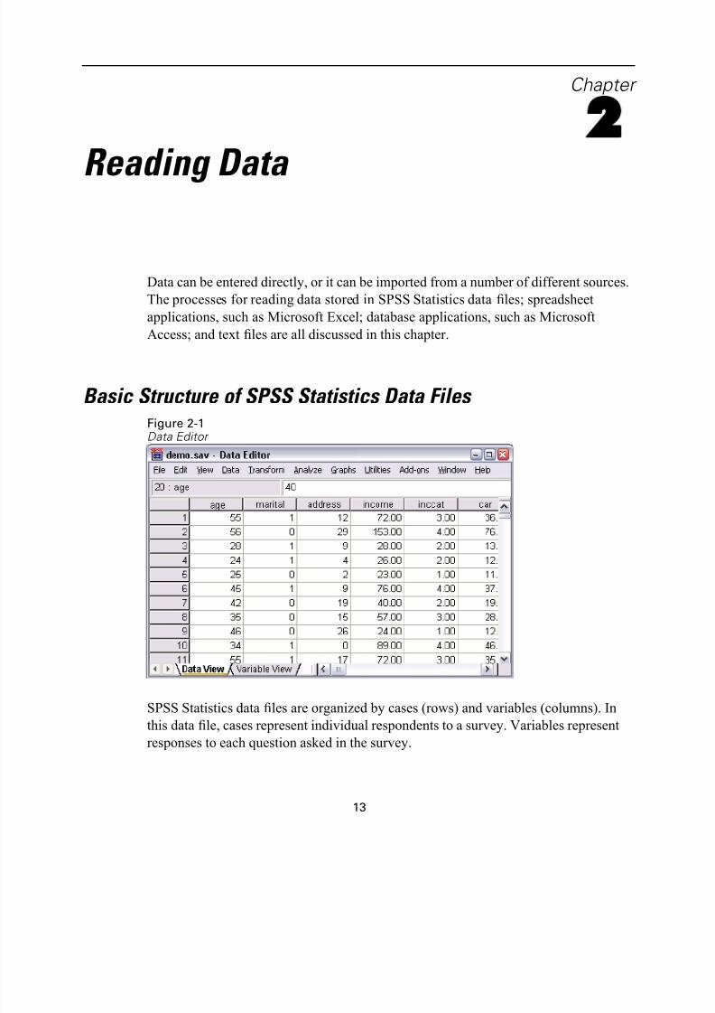
Basic Structure of SPSS Statistics Data Files Figure 2-1Data Editor
SPSS Statistics data files are organized by cases (rows) and variables (columns). Inthis data file, cases represent individual respondents to a survey. Variables represen
responses to each question asked in the survey.
13
5/11/2018 SPSS Statistics Brief Guide 17.0 - slidepdf.com
http://slidepdf.com/reader/full/spss-statistics-brief-guide-170-55a2339b08a28 28/224
14
Chapter 2
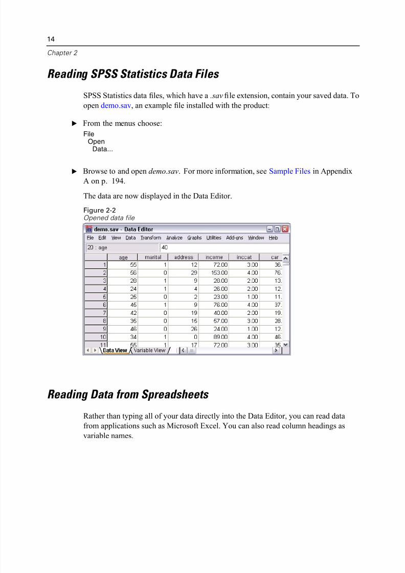
Reading SPSS Statistics Data Files
SPSS Statistics data files, which have a .sav file extension, contain your saved data.
open demo.sav, an example file installed with the product:
E From the menus choose:
FileOpen
Data...
E Browse to and open demo.sav. For more information, see Sample Files in Appendi
A on p. 194.
The data are now displayed in the Data Editor.Figure 2-2Opened data file
Reading Data from Spreadsheets Rather than typing all of your data directly into the Data Editor, you can read data
from applications such as Microsoft Excel. You can also read column headings as
variable names.
5/11/2018 SPSS Statistics Brief Guide 17.0 - slidepdf.com
http://slidepdf.com/reader/full/spss-statistics-brief-guide-170-55a2339b08a28 29/224
Reading D
E From the menus choose:
FileOpen
Data...
E Select Excel (*.xls) as the file type you want to view.
E Open demo.xls. For more information, see Sample Files in Appendix A on p. 194.
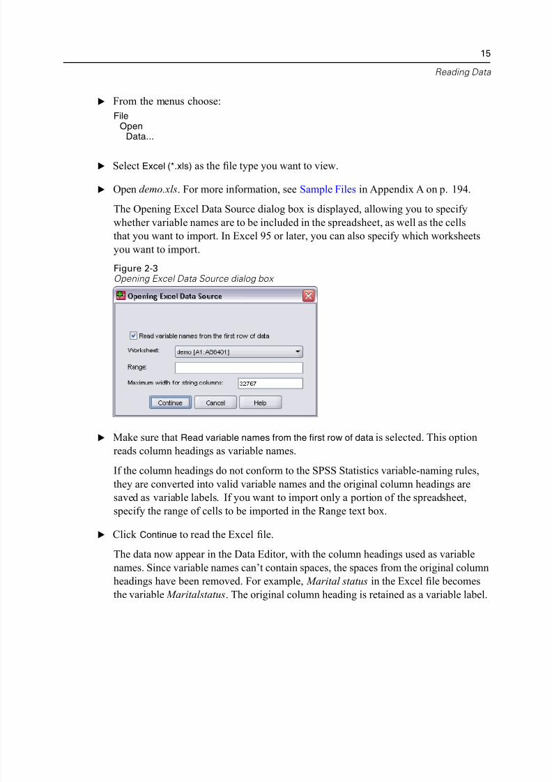
The Opening Excel Data Source dialog box is displayed, allowing you to specify
whether variable names are to be included in the spreadsheet, as well as the cells
that you want to import. In Excel 95 or later, you can also specify which worksheet
you want to import.
Figure 2-3Opening Excel Data Source dialog box
E Make sure that Read variable names from the first row of data is selected. This option
reads column headings as variable names.
If the column headings do not conform to the SPSS Statistics variable-naming rules
they are converted into valid variable names and the original column headings are
saved as variable labels. If you want to import only a portion of the spreadsheet,
specify the range of cells to be imported in the Range text box.
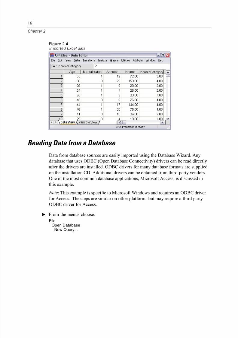
E Click Continue to read the Excel file.
The data now appear in the Data Editor, with the column headings used as variable
names. Since variable names can’t contain spaces, the spaces from the original colu
headings have been removed. For example, Marital status in the Excel file become
the variable Maritalstatus. The original column heading is retained as a variable lab
5/11/2018 SPSS Statistics Brief Guide 17.0 - slidepdf.com
http://slidepdf.com/reader/full/spss-statistics-brief-guide-170-55a2339b08a28 30/224
16
Chapter 2
Figure 2-4Imported Excel data
Reading Data from a Database
Data from database sources are easily imported using the Database Wizard. Any
database that uses ODBC (Open Database Connectivity) drivers can be read directl
after the drivers are installed. ODBC drivers for many database formats are supplie
on the installation CD. Additional drivers can be obtained from third-party vendors
One of the most common database applications, Microsoft Access, is discussed inthis example.
Note: This example is specific to Microsoft Windows and requires an ODBC driver
for Access. The steps are similar on other platforms but may require a third-party
ODBC driver for Access.
E From the menus choose:
FileOpen Database
New Query...
5/11/2018 SPSS Statistics Brief Guide 17.0 - slidepdf.com
http://slidepdf.com/reader/full/spss-statistics-brief-guide-170-55a2339b08a28 31/224
Reading D
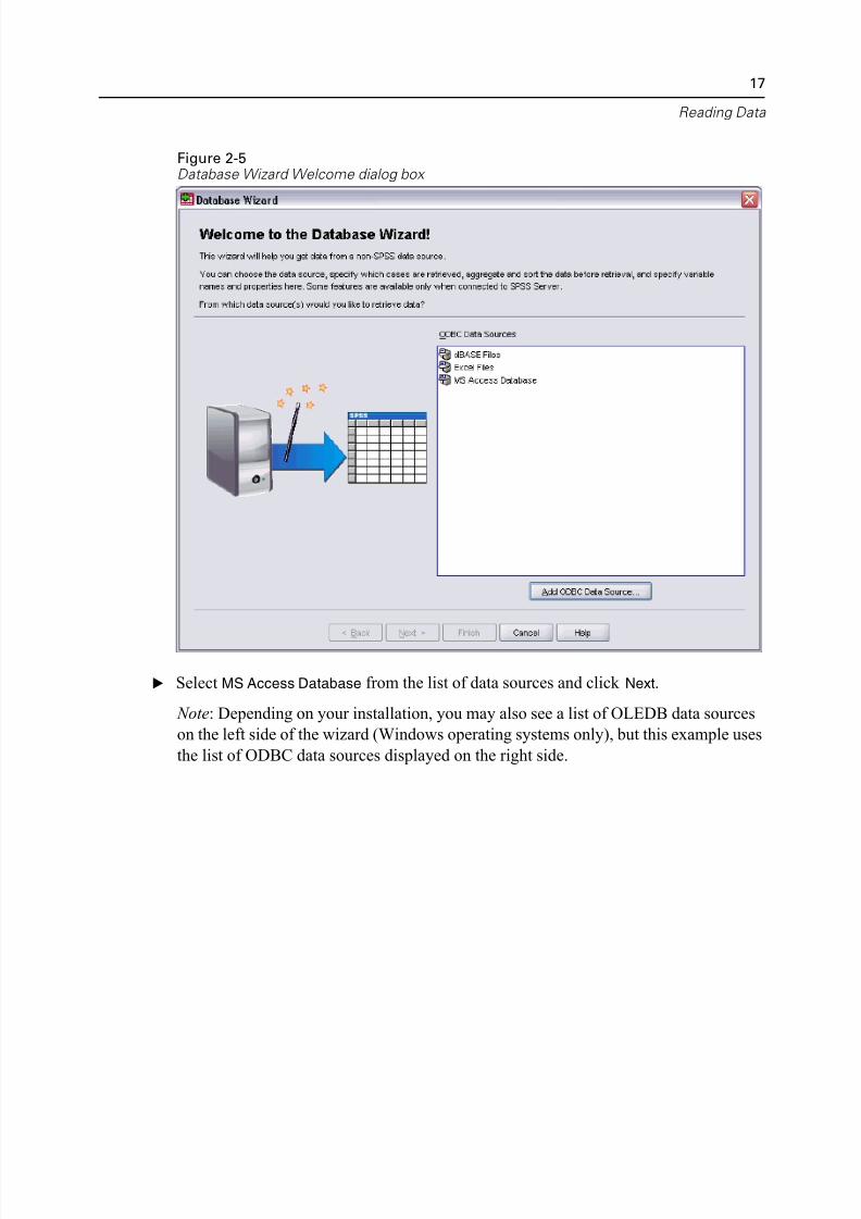
Figure 2-5Database Wizard Welcome dialog box
E Select MS Access Database from the list of data sources and click Next.
Note: Depending on your installation, you may also see a list of OLEDB data sourc
on the left side of the wizard (Windows operating systems only), but this example u
the list of ODBC data sources displayed on the right side.
5/11/2018 SPSS Statistics Brief Guide 17.0 - slidepdf.com
http://slidepdf.com/reader/full/spss-statistics-brief-guide-170-55a2339b08a28 32/224
18
Chapter 2
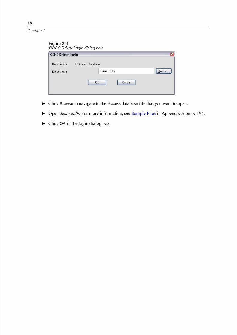
Figure 2-6ODBC Driver Login dialog box
E Click Browse to navigate to the Access database file that you want to open.
E Open demo.mdb. For more information, see Sample Files in Appendix A on p. 194
E Click OK in the login dialog box.
5/11/2018 SPSS Statistics Brief Guide 17.0 - slidepdf.com
http://slidepdf.com/reader/full/spss-statistics-brief-guide-170-55a2339b08a28 33/224
Reading D
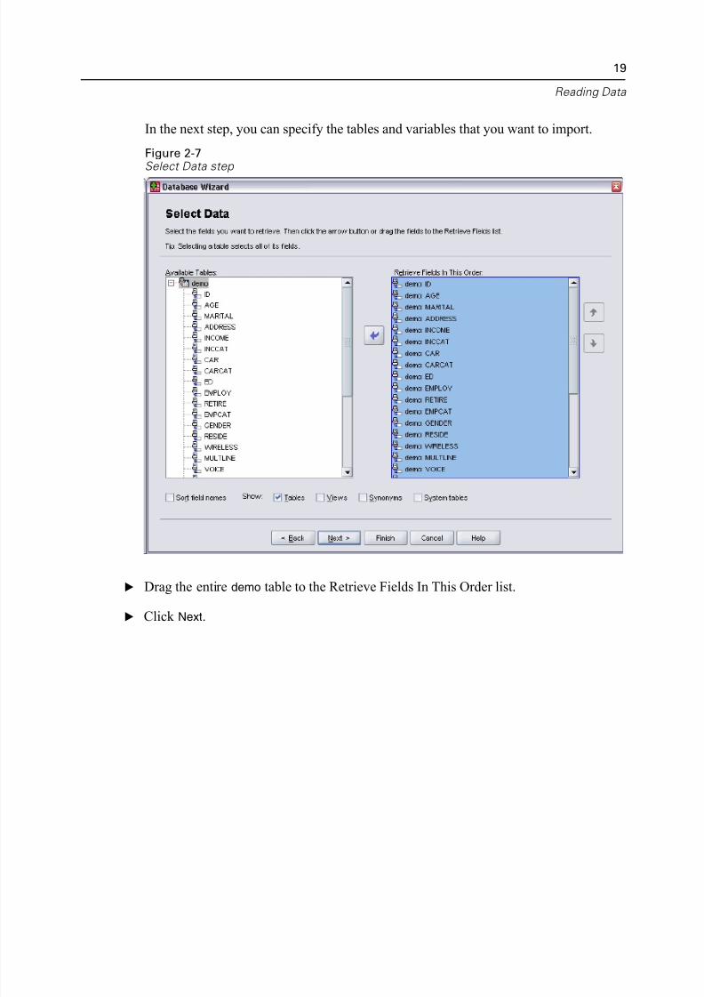
In the next step, you can specify the tables and variables that you want to import.
Figure 2-7Select Data step
E Drag the entire demo table to the Retrieve Fields In This Order list.
E Click Next.
5/11/2018 SPSS Statistics Brief Guide 17.0 - slidepdf.com
http://slidepdf.com/reader/full/spss-statistics-brief-guide-170-55a2339b08a28 34/224
20
Chapter 2
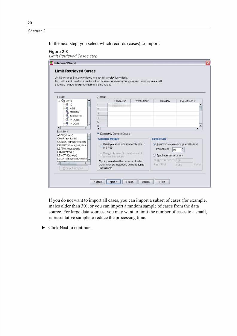
In the next step, you select which records (cases) to import.
Figure 2-8Limit Retrieved Cases step
If you do not want to import all cases, you can import a subset of cases (for exampl
males older than 30), or you can import a random sample of cases from the data
source. For large data sources, you may want to limit the number of cases to a smal
representative sample to reduce the processing time.
E Click Next to continue.
5/11/2018 SPSS Statistics Brief Guide 17.0 - slidepdf.com
http://slidepdf.com/reader/full/spss-statistics-brief-guide-170-55a2339b08a28 35/224
Reading D
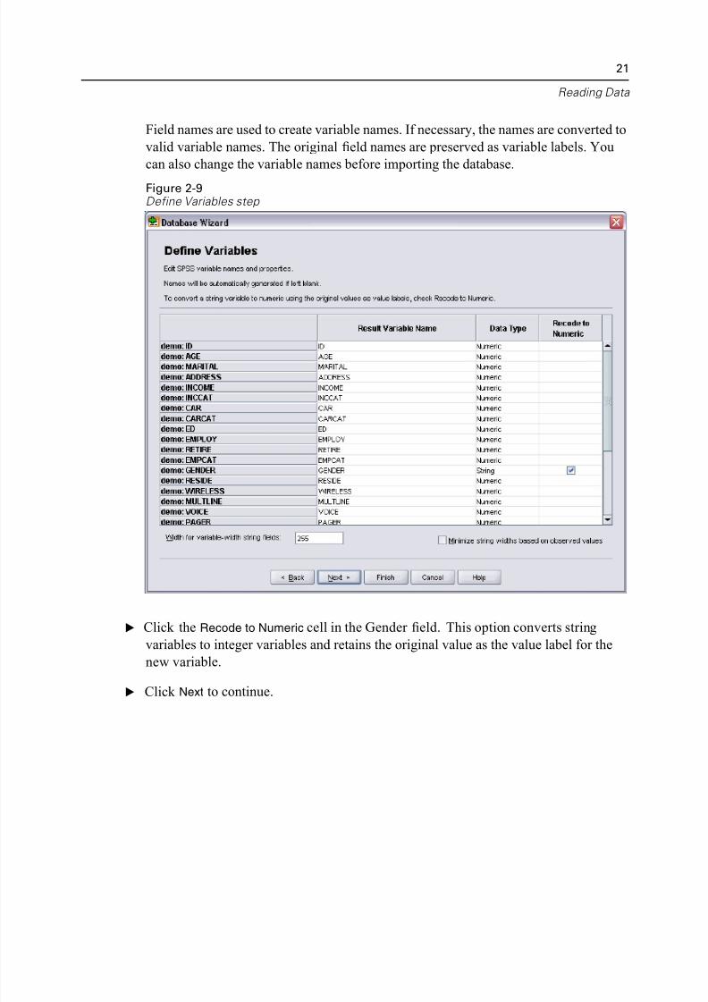
Field names are used to create variable names. If necessary, the names are converted
valid variable names. The original field names are preserved as variable labels. You
can also change the variable names before importing the database.
Figure 2-9Define Variables step
E Click the Recode to Numeric cell in the Gender field. This option converts string
variables to integer variables and retains the original value as the value label for the
new var iable.
E Click Next to continue.
5/11/2018 SPSS Statistics Brief Guide 17.0 - slidepdf.com
http://slidepdf.com/reader/full/spss-statistics-brief-guide-170-55a2339b08a28 36/224
22
Chapter 2
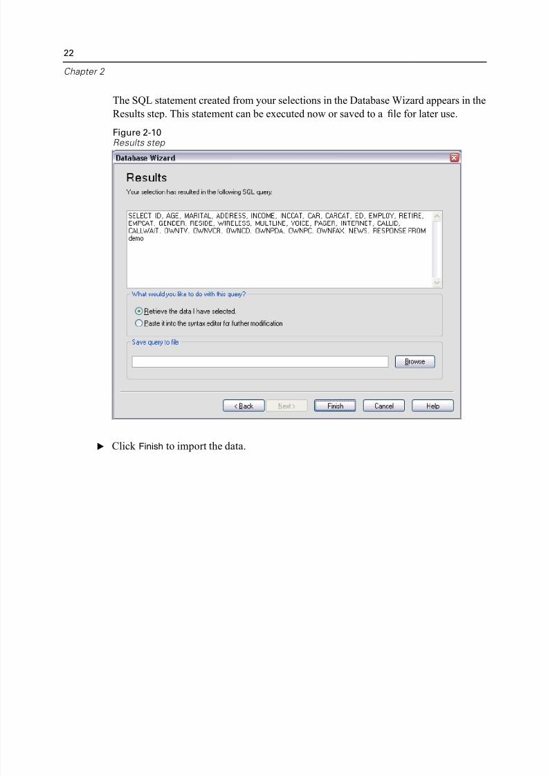
The SQL statement created from your selections in the Database Wizard appears in
Results step. This statement can be executed now or saved to a file for later use.
Figure 2-10Results step
E Click Finish to import the data.
5/11/2018 SPSS Statistics Brief Guide 17.0 - slidepdf.com
http://slidepdf.com/reader/full/spss-statistics-brief-guide-170-55a2339b08a28 37/224
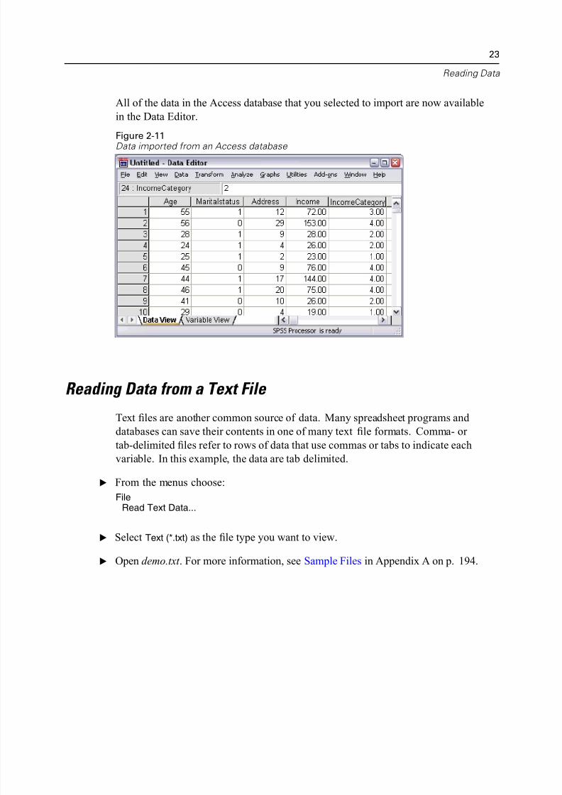
Reading D
All of the data in the Access database that you selected to import are now available
in the Data Editor.
Figure 2-11Data imported from an Access database
Reading Data from a Text File
Text files are another common source of data. Many spreadsheet programs anddatabases can save their contents in one of many text file formats. Comma- or
tab-delimited files refer to rows of data that use commas or tabs to indicate each
variable. In this example, the data are tab delimited.
E From the menus choose:
FileRead Text Data...
E Select Text (*.txt) as the file type you want to view.
E Open demo.txt . For more information, see Sample Files in Appendix A on p. 194.
5/11/2018 SPSS Statistics Brief Guide 17.0 - slidepdf.com
http://slidepdf.com/reader/full/spss-statistics-brief-guide-170-55a2339b08a28 38/224
24
Chapter 2
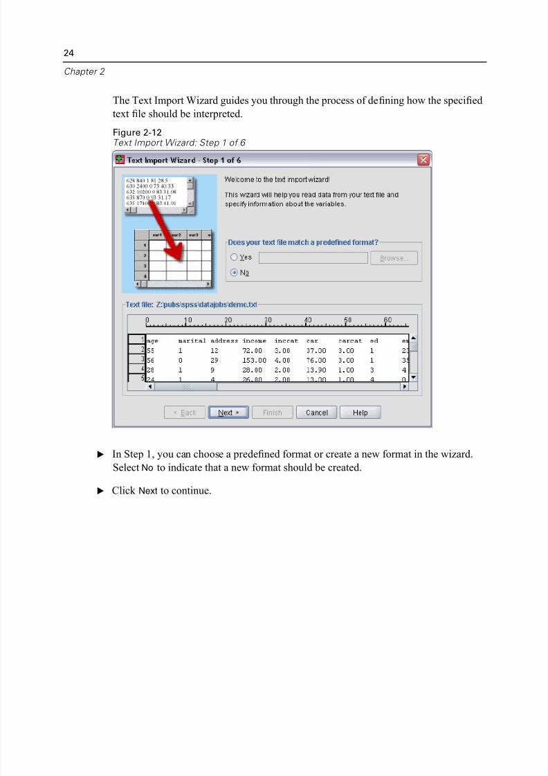
The Text Import Wizard guides you through the process of defining how the specifi
text file should be interpreted.
Figure 2-12Text Import Wizard: Step 1 of 6
E In Step 1, you can choose a predefined format or create a new format in the wizard
Select No to indicate that a new format should be created.
E Click Next to continue.
5/11/2018 SPSS Statistics Brief Guide 17.0 - slidepdf.com
http://slidepdf.com/reader/full/spss-statistics-brief-guide-170-55a2339b08a28 39/224
Reading D
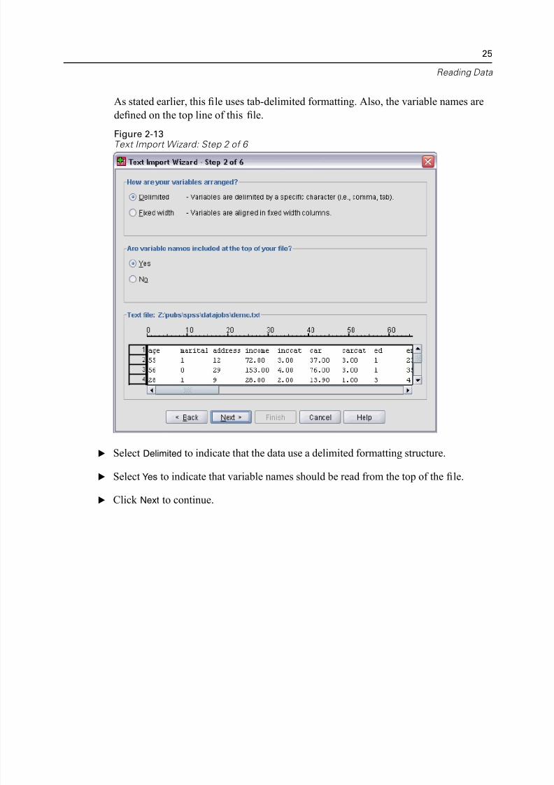
As stated earlier, this file uses tab-delimited formatting. Also, the variable names ar
defined on the top line of this file.
Figure 2-13Text Import Wizard: Step 2 of 6
E Select Delimited to indicate that the data use a delimited formatting structure.
E Select Yes to indicate that variable names should be read from the top of the file.
E Click Next to continue.
5/11/2018 SPSS Statistics Brief Guide 17.0 - slidepdf.com
http://slidepdf.com/reader/full/spss-statistics-brief-guide-170-55a2339b08a28 40/224
26
Chapter 2
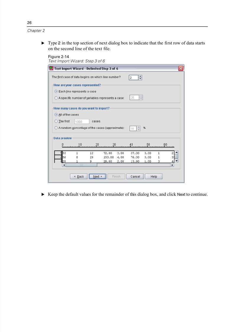
E Type 2 in the top section of next dialog box to indicate that the first row of data star
on the second line of the text file.
Figure 2-14Text Import Wizard: Step 3 of 6
E Keep the default values for the remainder of this dialog box, and click Next to contin
5/11/2018 SPSS Statistics Brief Guide 17.0 - slidepdf.com
http://slidepdf.com/reader/full/spss-statistics-brief-guide-170-55a2339b08a28 41/224
Reading D
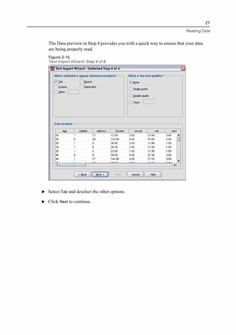
The Data preview in Step 4 provides you with a quick way to ensure that your data
are being properly read.
Figure 2-15Text Import Wizard: Step 4 of 6
E Select Tab and deselect the other options.
E Click Next to continue.
5/11/2018 SPSS Statistics Brief Guide 17.0 - slidepdf.com
http://slidepdf.com/reader/full/spss-statistics-brief-guide-170-55a2339b08a28 42/224
28
Chapter 2
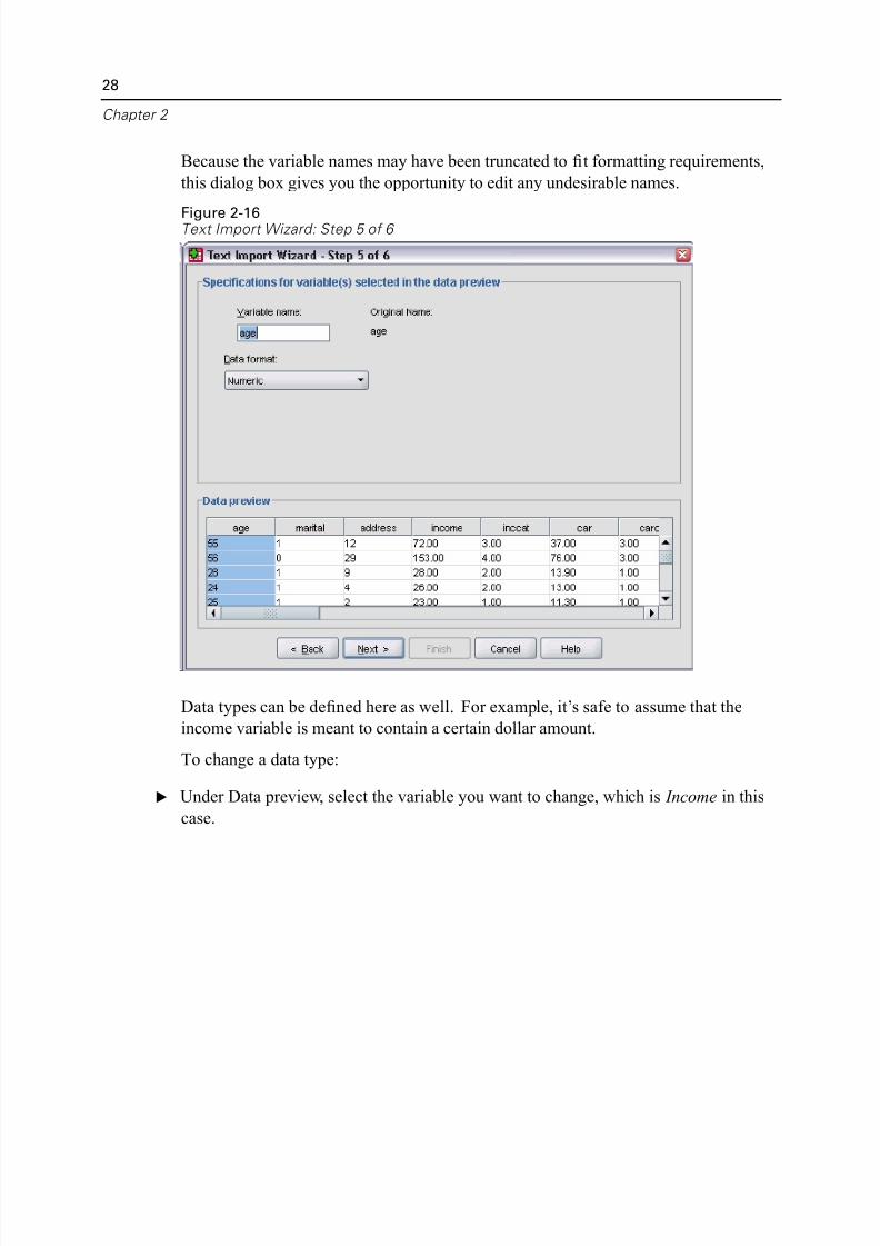
Because the variable names may have been truncated to fit formatting requirements
this dialog box gives you the opportunity to edit any undesirable names.
Figure 2-16Text Import Wizard: Step 5 of 6
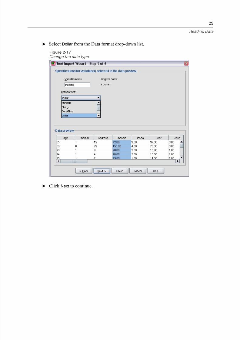
Data types can be defined here as well. For example, it’s safe to assume that the
income variable is meant to contain a certain dollar amount.
To change a data type:
E Under Data preview, select the variable you want to change, which is Income in thi
case.
5/11/2018 SPSS Statistics Brief Guide 17.0 - slidepdf.com
http://slidepdf.com/reader/full/spss-statistics-brief-guide-170-55a2339b08a28 43/224
Reading D
E Select Dollar from the Data format drop-down list.
Figure 2-17Change the data type
E Click Next to continue.
5/11/2018 SPSS Statistics Brief Guide 17.0 - slidepdf.com
http://slidepdf.com/reader/full/spss-statistics-brief-guide-170-55a2339b08a28 44/224
30
Chapter 2
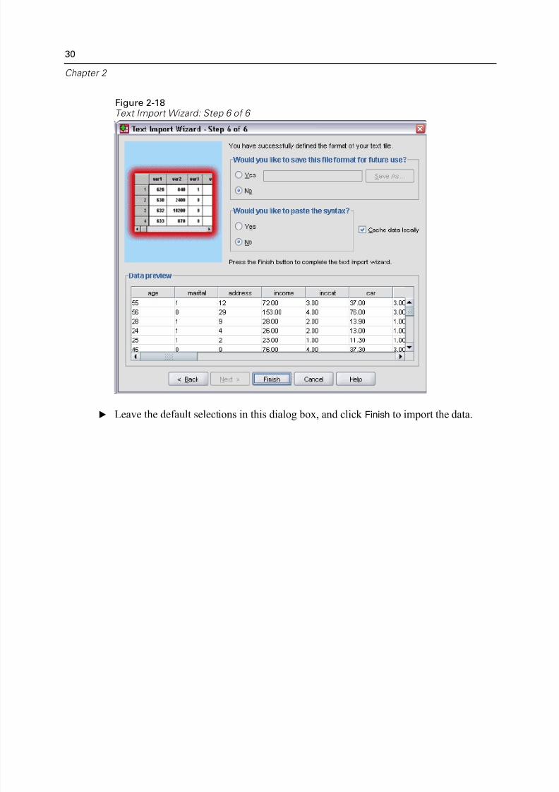
Figure 2-18Text Import Wizard: Step 6 of 6
E Leave the default selections in this dialog box, and click Finish to import the data.
5/11/2018 SPSS Statistics Brief Guide 17.0 - slidepdf.com
http://slidepdf.com/reader/full/spss-statistics-brief-guide-170-55a2339b08a28 45/224
Chapt
3
Using the Data Editor
The Data Editor displays the contents of the active data file. The information in the
Data Editor consists of variables and cases.
In Data View, columns represent variables, and rows represent cases (observatio
In Variable View, each row is a variable, and each column is an attribute that is
associated with that variable.
Variables are used to represent the different types of data that you have compiled. A
common analogy is that of a survey. The response to each question on a survey is
equivalent to a variable. Variables come in many different types, including number
strings, currency, and dates.
Entering Numeric Data
Data can be entered into the Data Editor, which may be useful for small data files o
for making minor edits to larger data files.
E Click the Variable View tab at the bottom of the Data Editor window.
You need to define the variables that will be used. In this case, only three variables
needed: age, marital status, and income.
31
5/11/2018 SPSS Statistics Brief Guide 17.0 - slidepdf.com
http://slidepdf.com/reader/full/spss-statistics-brief-guide-170-55a2339b08a28 46/224
32
Chapter 3
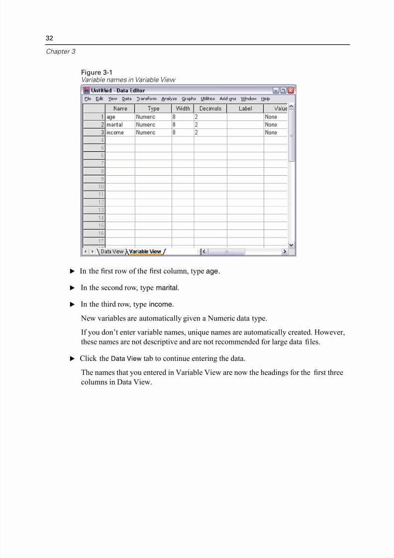
Figure 3-1Variable names in Variable View
E In the first row of the first column, type age.
E In the second row, type marital.
E In the third row, type income.
New variables are automatically given a Numeric data type.
If you don’t enter variable names, unique names are automatically created. Howeve
these names are not descriptive and are not recommended for large data files.
E Click the Data View tab to continue entering the data.
The names that you entered in Variable View are now the headings for the first thre
columns in Data View.
5/11/2018 SPSS Statistics Brief Guide 17.0 - slidepdf.com
http://slidepdf.com/reader/full/spss-statistics-brief-guide-170-55a2339b08a28 47/224
Using the Data Ed
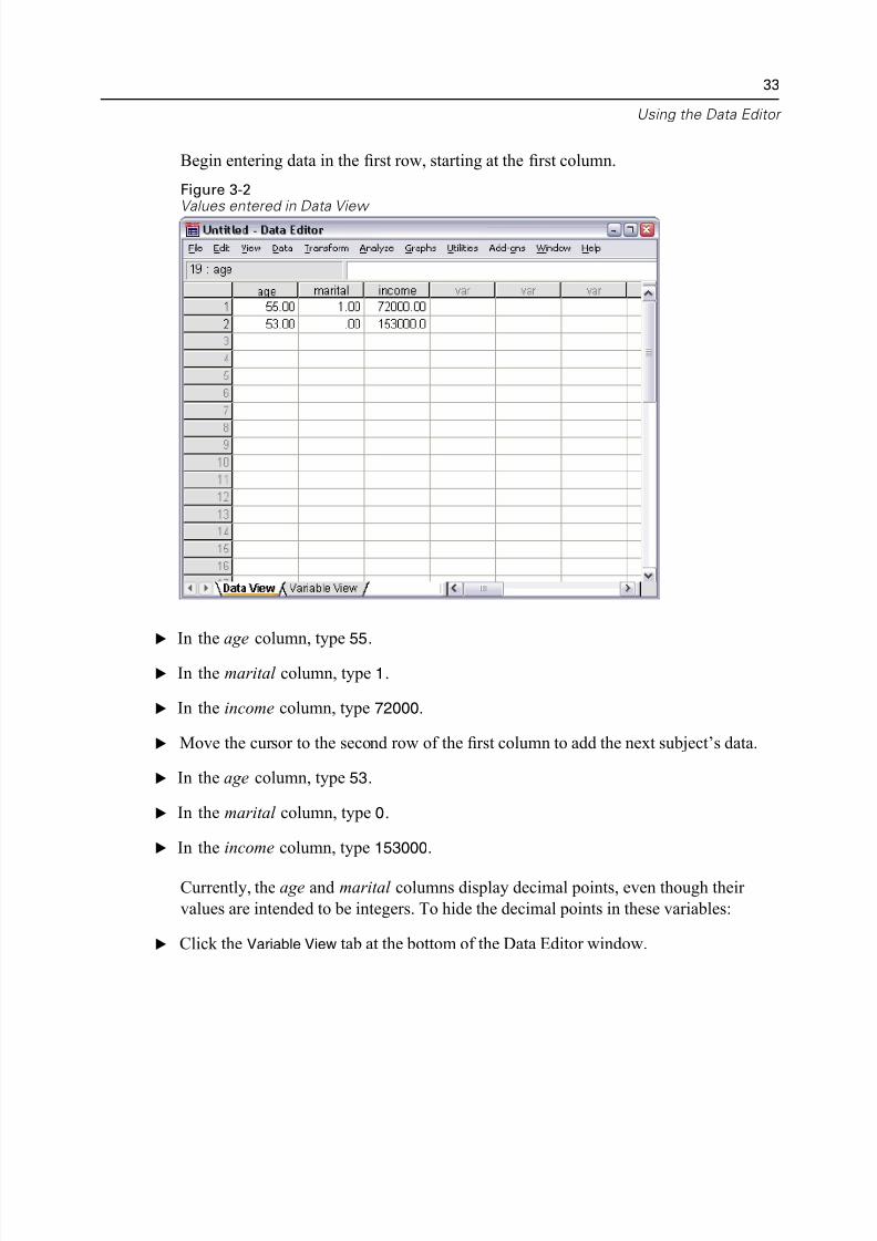
Begin entering data in the first row, starting at the first column.
Figure 3-2Values entered in Data View
E In the age column, type 55.
E In the marital column, type 1.
E In the income column, type 72000.
E Move the cursor to the second row of the first column to add the next subject’s data
E In the age column, type 53.
E In the marital column, type 0.
E In the income column, type 153000.
Currently, the age and marital columns display decimal points, even though their
values are intended to be integers. To hide the decimal points in these variables:
E Click the Variable View tab at the bottom of the Data Editor window.
5/11/2018 SPSS Statistics Brief Guide 17.0 - slidepdf.com
http://slidepdf.com/reader/full/spss-statistics-brief-guide-170-55a2339b08a28 48/224
34
Chapter 3
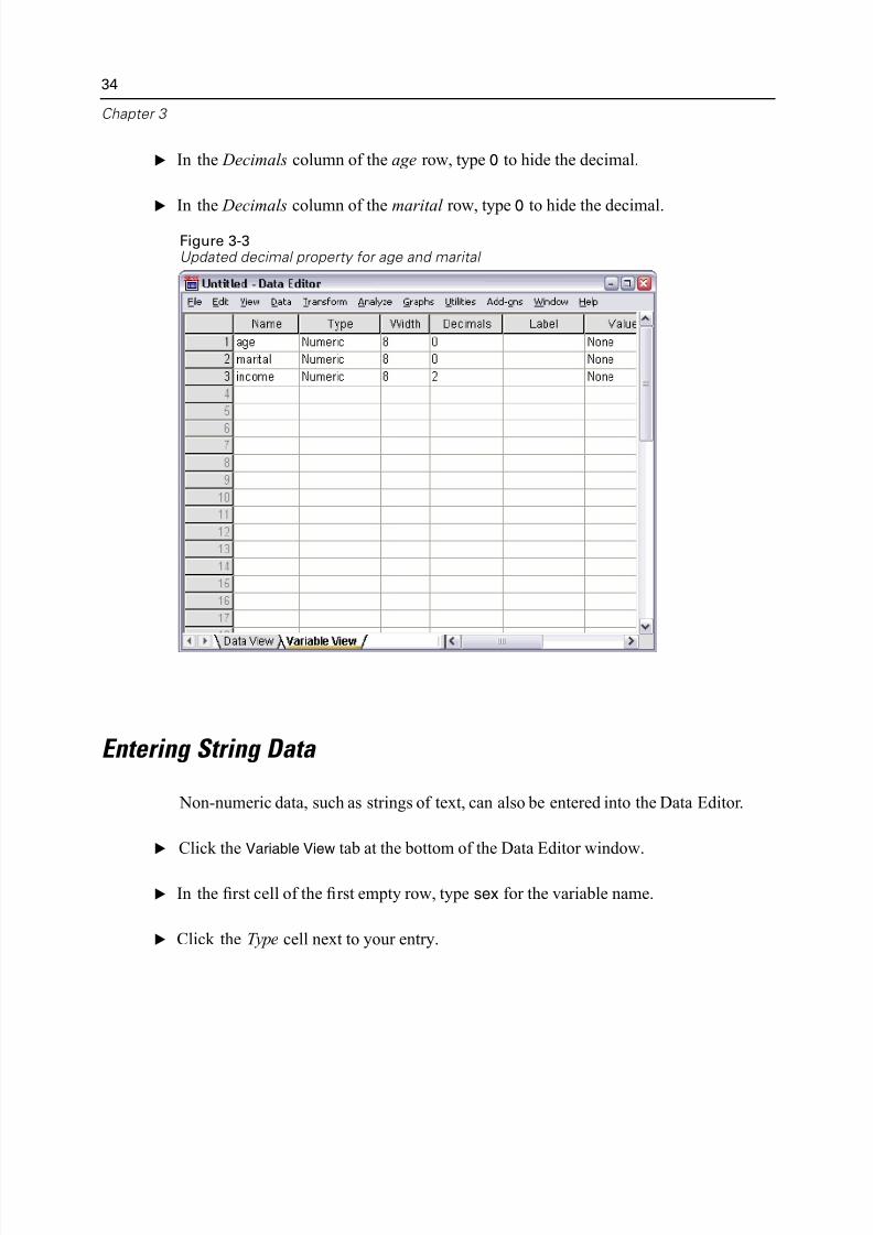
E In the Decimals column of the age row, type 0 to hide the decimal.
E In the Decimals column of the marital row, type 0 to hide the decimal.
Figure 3-3Updated decimal property for age and marital
Entering String Data
Non-numeric data, such as strings of text, can also be entered into the Data Editor.
E Click the Variable View tab at the bottom of the Data Editor window.
E In the first cell of the first empty row, type sex for the variable name.
E Click the Type cell next to your entry.
5/11/2018 SPSS Statistics Brief Guide 17.0 - slidepdf.com
http://slidepdf.com/reader/full/spss-statistics-brief-guide-170-55a2339b08a28 49/224
Using the Data Ed
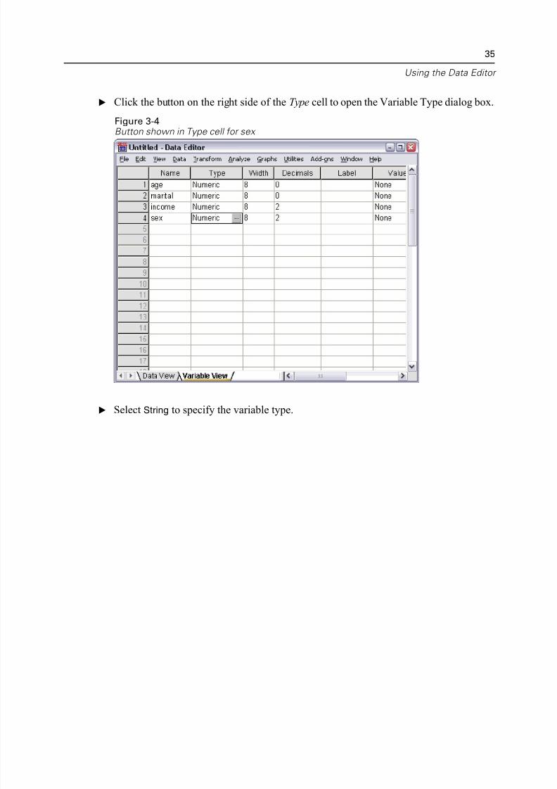
E Click the button on the right side of the Type cell to open the Variable Type dialog b
Figure 3-4Button shown in Type cell for sex
E Select String to specify the variable type.
5/11/2018 SPSS Statistics Brief Guide 17.0 - slidepdf.com
http://slidepdf.com/reader/full/spss-statistics-brief-guide-170-55a2339b08a28 50/224
36
Chapter 3
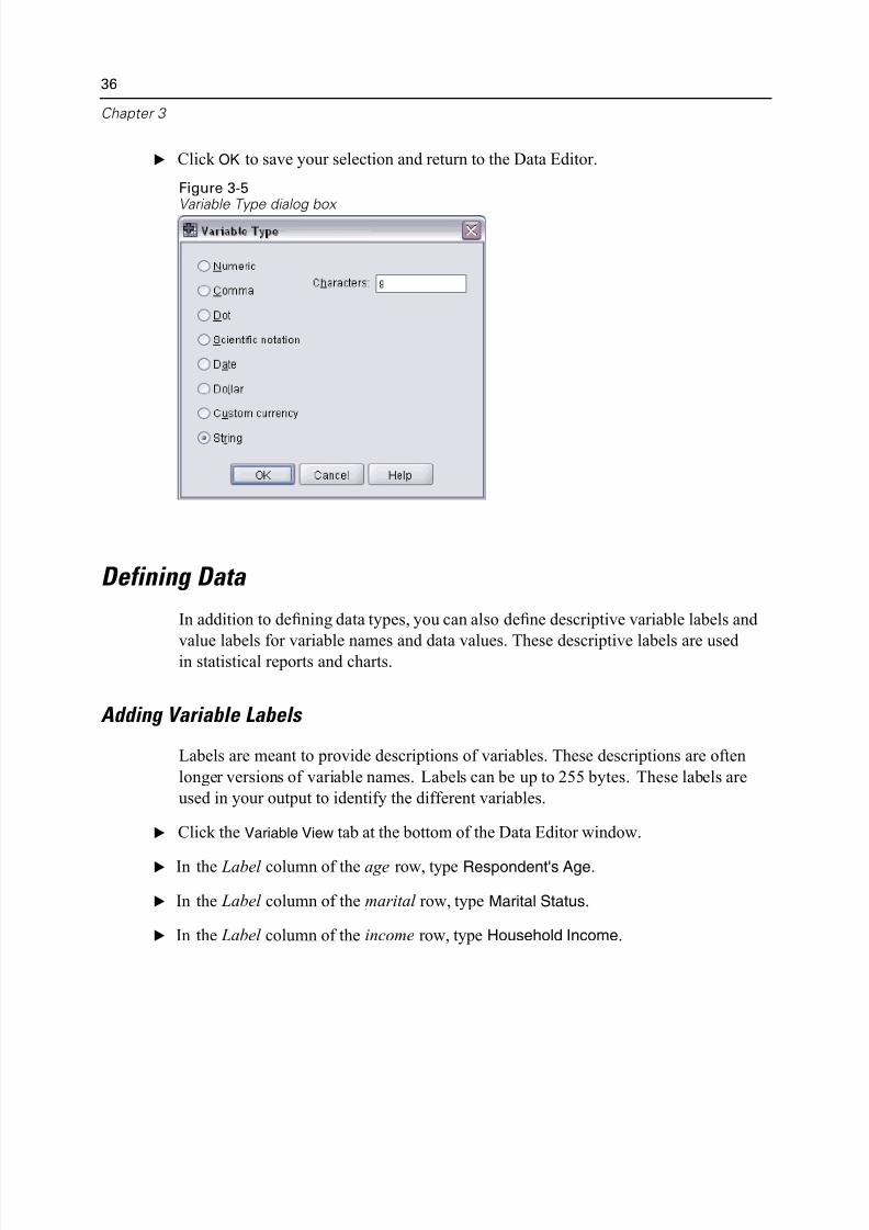
E Click OK to save your selection and return to the Data Editor.
Figure 3-5Variable Type dialog box
Defining Data
In addition to defining data types, you can also define descriptive variable labels an
value labels for variable names and data values. These descriptive labels are usedin statistical reports and charts.
Adding Variable Labels
Labels are meant to provide descriptions of variables. These descriptions are often
longer versions of variable names. Labels can be up to 255 bytes. These labels are
used in your output to identify the different variables.
E Click the Variable View tab at the bottom of the Data Editor window.
E In the Label column of the age row, type Respondent's Age.
E In the Label column of the marital row, type Marital Status.
E In the Label column of the income row, type Household Income.
5/11/2018 SPSS Statistics Brief Guide 17.0 - slidepdf.com
http://slidepdf.com/reader/full/spss-statistics-brief-guide-170-55a2339b08a28 51/224
Using the Data Ed
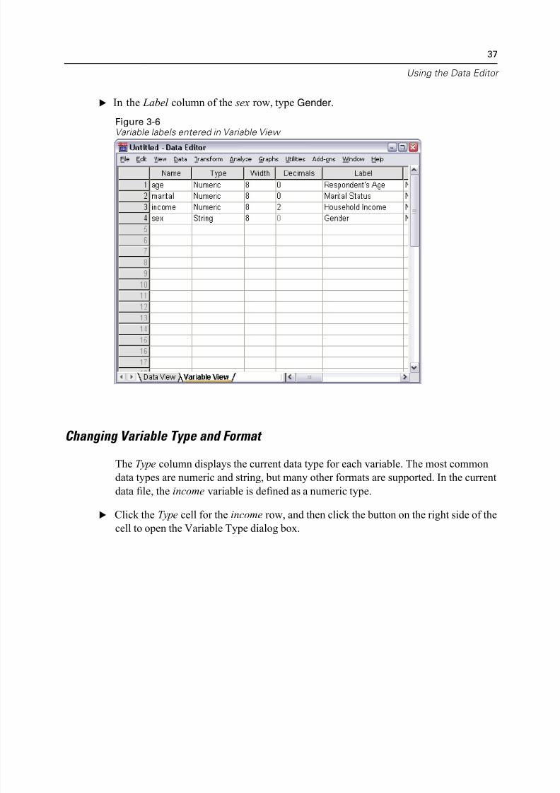
E In the Label column of the sex row, type Gender.
Figure 3-6Variable labels entered in Variable View
Changing Variable Type and Format
The Type column displays the current data type for each variable. The most commo
data types are numeric and string, but many other formats are supported. In the curr
data file, the income variable is defined as a numeric type.
E Click the Type cell for the income row, and then click the button on the right side of
cell to open the Variable Type dialog box.
5/11/2018 SPSS Statistics Brief Guide 17.0 - slidepdf.com
http://slidepdf.com/reader/full/spss-statistics-brief-guide-170-55a2339b08a28 52/224
38
Chapter 3
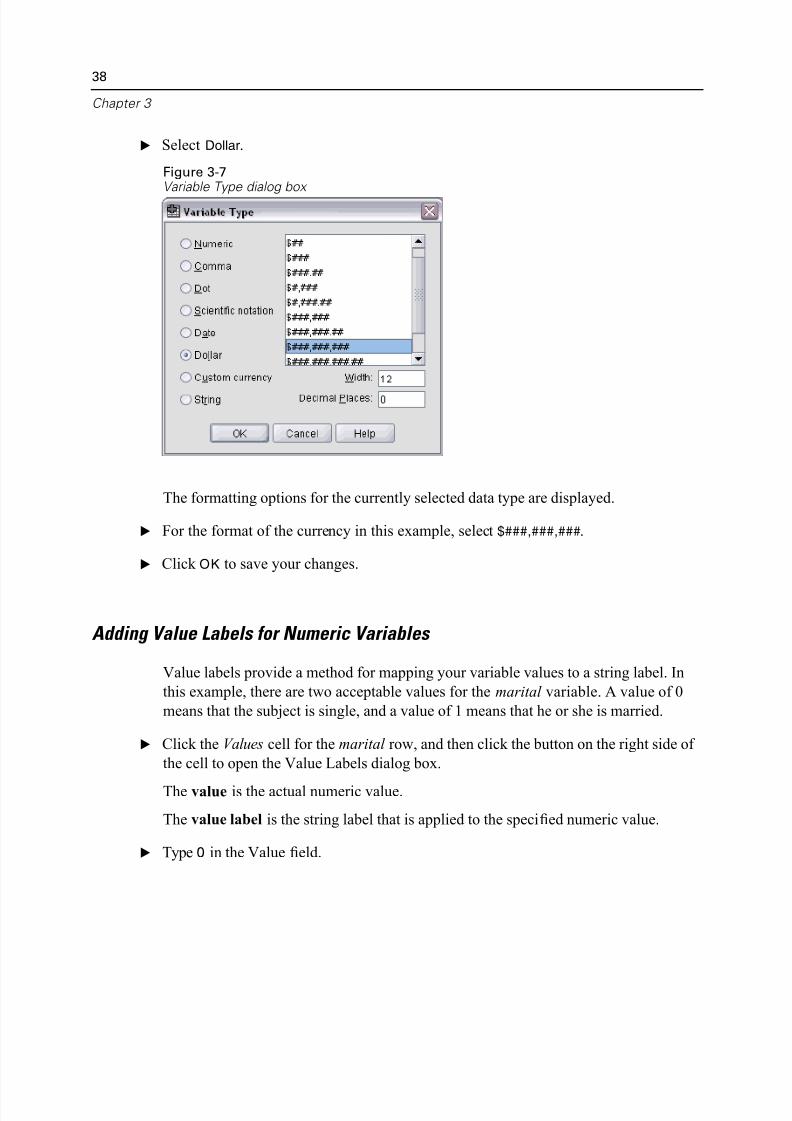
E Select Dollar.
Figure 3-7Variable Type dialog box
The formatting options for the currently selected data type are displayed.
E For the format of the currency in this example, select $###,###,###.
E Click OK to save your changes.
Adding Value Labels for Numeric Variables
Value labels provide a method for mapping your variable values to a string label. In
this example, there are two acceptable values for the marital variable. A value of 0
means that the subject is single, and a value of 1 means that he or she is married.
E Click the Values cell for the marital row, and then click the button on the right side
the cell to open the Value Labels dialog box.
The value is the actual numeric value.
The value label is the string label that is applied to the specified numeric value.
E Type 0 in the Value field.
5/11/2018 SPSS Statistics Brief Guide 17.0 - slidepdf.com
http://slidepdf.com/reader/full/spss-statistics-brief-guide-170-55a2339b08a28 53/224
Using the Data Ed
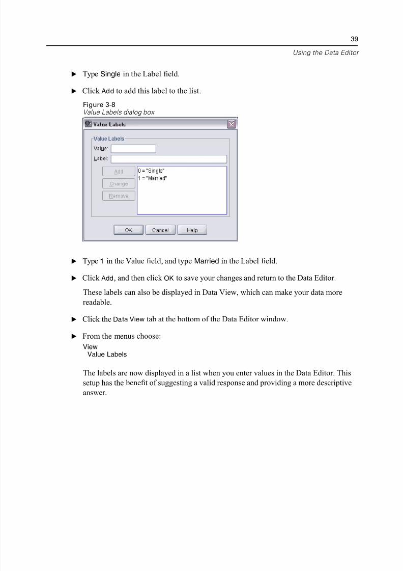
E Type Single in the Label field.
E Click Add to add this label to the list.
Figure 3-8Value Labels dialog box
E Type 1 in the Value field, and type Married in the Label field.
E Click Add, and then click OK to save your changes and return to the Data Editor.
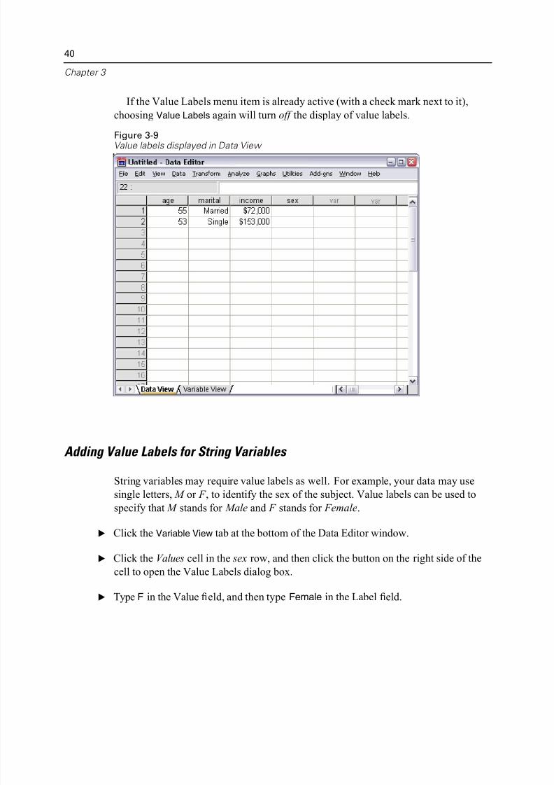
These labels can also be displayed in Data View, which can make your data more
readable.
E Click the Data View tab at the bottom of the Data Editor window.
E From the menus choose:
ViewValue Labels
The labels are now displayed in a list when you enter values in the Data Editor. Th
setup has the benefit of suggesting a valid response and providing a more descriptiv
answer.
5/11/2018 SPSS Statistics Brief Guide 17.0 - slidepdf.com
http://slidepdf.com/reader/full/spss-statistics-brief-guide-170-55a2339b08a28 54/224
40
Chapter 3
If the Value Labels menu item is already active (with a check mark next to it),
choosing Value Labels again will turn off the display of value labels.
Figure 3-9Value labels displayed in Data View
Adding Value Labels for String Variables
String variables may require value labels as well. For example, your data may use
single letters, M or F , to identify the sex of the subject. Value labels can be used to
specify that M stands for Male and F stands for Female.
E Click the Variable View tab at the bottom of the Data Editor window.
E Click the Values cell in the sex row, and then click the button on the right side of th
cell to open the Value Labels dialog box.
E Type F in the Value field, and then type Female in the Label field.
5/11/2018 SPSS Statistics Brief Guide 17.0 - slidepdf.com
http://slidepdf.com/reader/full/spss-statistics-brief-guide-170-55a2339b08a28 55/224
Using the Data Ed
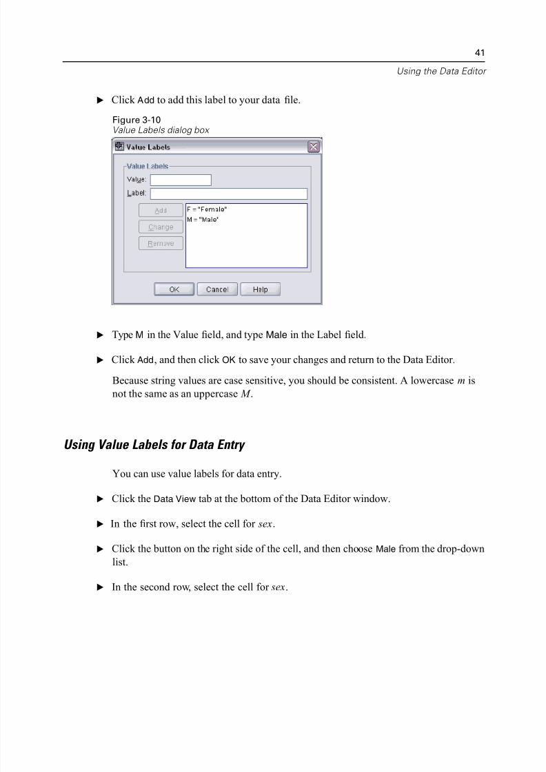
E Click Add to add this label to your data file.
Figure 3-10
Value Labels dialog box
E Type M in the Value field, and type Male in the Label field.
E Click Add, and then click OK to save your changes and return to the Data Editor.
Because string values are case sensitive, you should be consistent. A lowercase m i
not the same as an uppercase M .
Using Value Labels for Data Entry
You can use value labels for data entry.
E Click the Data View tab at the bottom of the Data Editor window.
E In the first row, select the cell for sex.
E Click the button on the right side of the cell, and then choose Male from the drop-do
list.
E In the second row, select the cell for sex.
5/11/2018 SPSS Statistics Brief Guide 17.0 - slidepdf.com
http://slidepdf.com/reader/full/spss-statistics-brief-guide-170-55a2339b08a28 56/224
42
Chapter 3
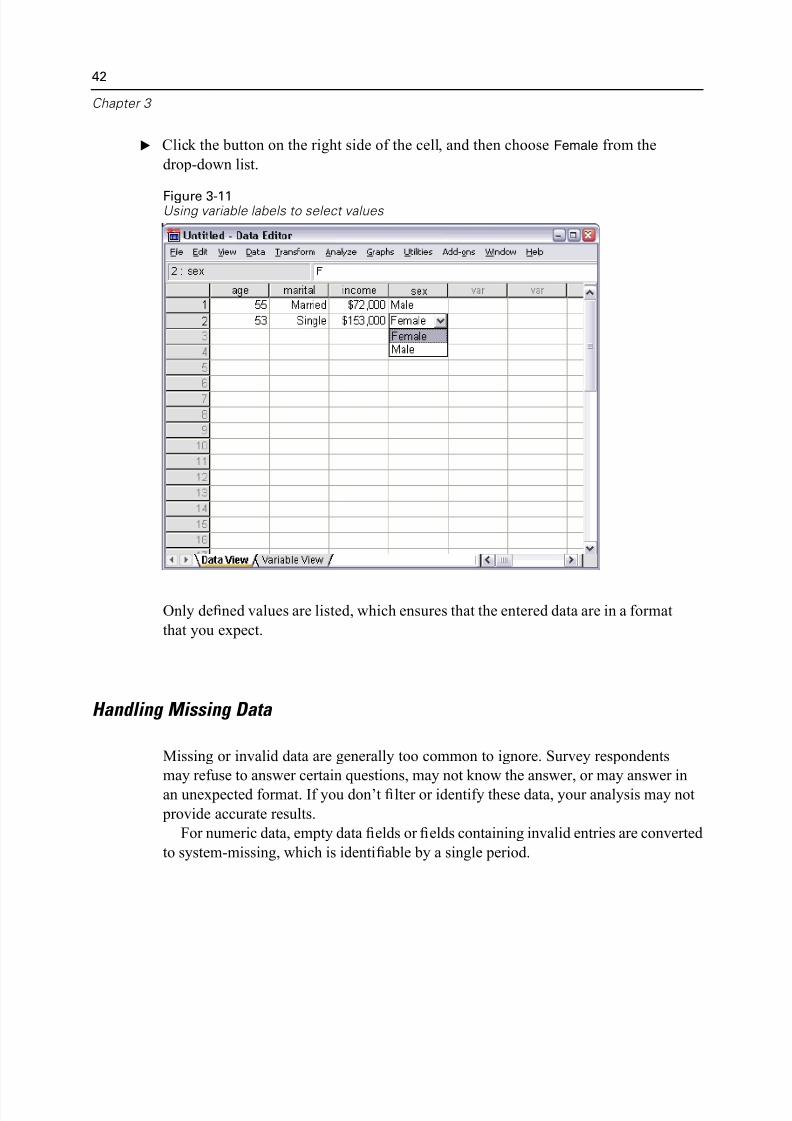
E Click the button on the right side of the cell, and then choose Female from the
drop-down list.
Figure 3-11Using variable labels to select values
Only defined values are listed, which ensures that the entered data are in a format
that you expect.
Handling Missing Data
Missing or invalid data are generally too common to ignore. Survey respondents
may refuse to answer certain questions, may not know the answer, or may answer inan unexpected format. If you don’t filter or identify these data, your analysis may n
provide accurate results.
For numeric data, empty data fields or fields containing invalid entries are conver
to system-missing, which is identifiable by a single period.
5/11/2018 SPSS Statistics Brief Guide 17.0 - slidepdf.com
http://slidepdf.com/reader/full/spss-statistics-brief-guide-170-55a2339b08a28 57/224
Using the Data Ed
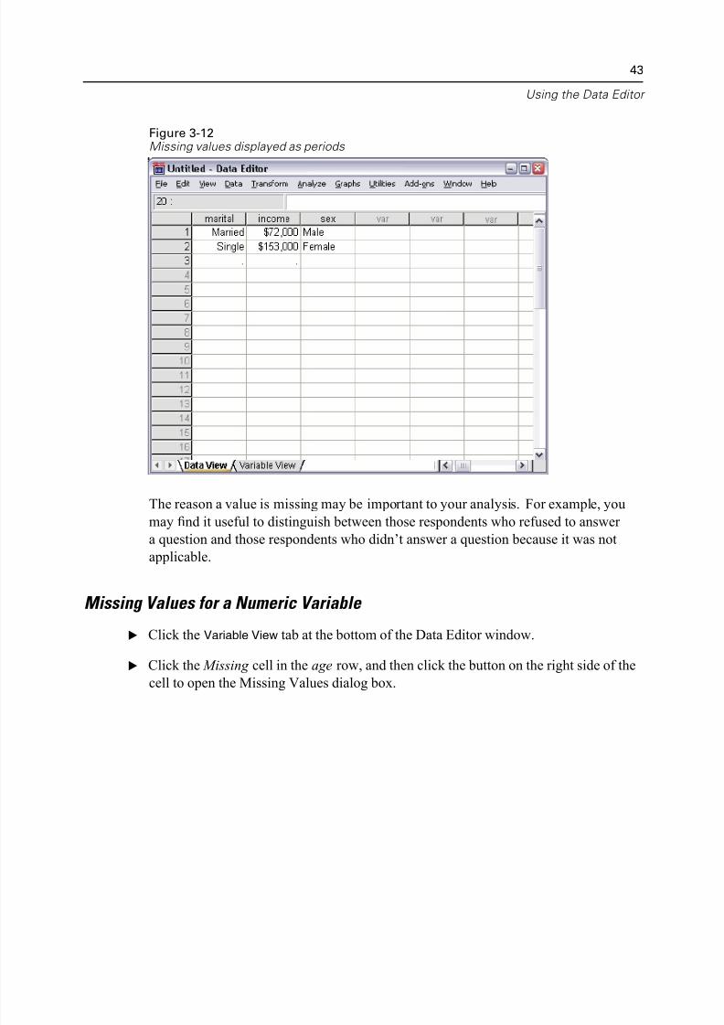
Figure 3-12Missing values displayed as periods
The reason a value is missing may be important to your analysis. For example, you
may find it useful to distinguish between those respondents who refused to answer
a question and those respondents who didn’t answer a question because it was notapplicable.
Missing Values for a Numeric Variable
E Click the Variable View tab at the bottom of the Data Editor window.
E Click the Missing cell in the age row, and then click the button on the right side of t
cell to open the Missing Values dialog box.
5/11/2018 SPSS Statistics Brief Guide 17.0 - slidepdf.com
http://slidepdf.com/reader/full/spss-statistics-brief-guide-170-55a2339b08a28 58/224
44
Chapter 3
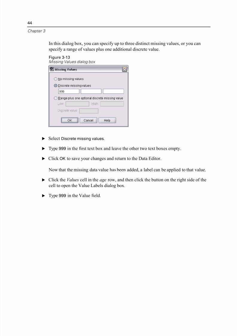
In this dialog box, you can specify up to three distinct missing values, or you can
specify a range of values plus one additional discrete value.
Figure 3-13Missing Values dialog box
E Select Discrete missing values.
E Type 999 in the first text box and leave the other two text boxes empty.
E Click OK to save your changes and return to the Data Editor.
Now that the missing data value has been added, a label can be applied to that value
E Click the Values cell in the age row, and then click the button on the right side of th
cell to open the Value Labels dialog box.
E Type 999 in the Value field.

5/11/2018 SPSS Statistics Brief Guide 17.0 - slidepdf.com
http://slidepdf.com/reader/full/spss-statistics-brief-guide-170-55a2339b08a28 59/224
Using the Data Ed
E Type No Response in the Label field.
Figure 3-14Value Labels dialog box
E Click Add to add this label to your data file.
E Click OK to save your changes and return to the Data Editor.
Missing Values for a String Variable Missing values for string variables are handled similarly to the missing values for
numeric variables. However, unlike numeric variables, empty fields in string variab
are not designated as system-missing. Rather, they are interpreted as an empty strin
E Click the Variable View tab at the bottom of the Data Editor window.
E Click the Missing cell in the sex row, and then click the button on the right side of t
cell to open the Missing Values dialog box.
E Select Discrete missing values.
E Type NR in the first text box.
Missing values for string variables are case sensitive. So, a value of nr is not treate
as a missing value.
5/11/2018 SPSS Statistics Brief Guide 17.0 - slidepdf.com
http://slidepdf.com/reader/full/spss-statistics-brief-guide-170-55a2339b08a28 60/224
46
Chapter 3
E Click OK to save your changes and return to the Data Editor.
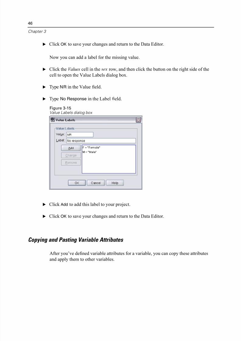
Now you can add a label for the missing value.
E Click the Values cell in the sex row, and then click the button on the right side of th
cell to open the Value Labels dialog box.
E Type NR in the Value field.
E Type No Response in the Label field.
Figure 3-15Value Labels dialog box
E Click Add to add this label to your project.
E Click OK to save your changes and return to the Data Editor.
Copying and Pasting Variable Attributes
After you’ve defined variable attributes for a variable, you can copy these attributes
and apply them to other variables.
5/11/2018 SPSS Statistics Brief Guide 17.0 - slidepdf.com
http://slidepdf.com/reader/full/spss-statistics-brief-guide-170-55a2339b08a28 61/224
Using the Data Ed
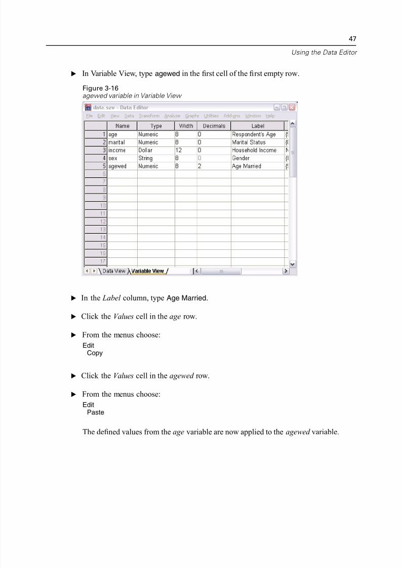
E In Variable View, type agewed in the first cell of the first empty row.
Figure 3-16
agewed variable in Variable View
E In the Label column, type Age Married.
E Click the Values cell in the age row.
E From the menus choose:
EditCopy
E Click the Values cell in the agewed row.
E From the menus choose:Edit
Paste
The defined values from the age variable are now applied to the agewed variable.
5/11/2018 SPSS Statistics Brief Guide 17.0 - slidepdf.com
http://slidepdf.com/reader/full/spss-statistics-brief-guide-170-55a2339b08a28 62/224
48
Chapter 3
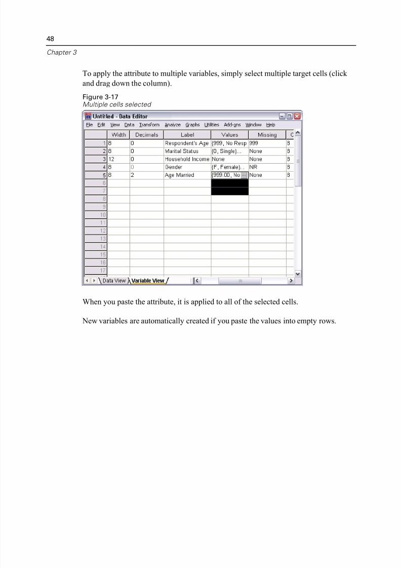
To apply the attribute to multiple variables, simply select multiple target cells (click
and drag down the column).
Figure 3-17Multiple cells selected
When you paste the attribute, it is applied to all of the selected cells.
New variables are automatically created if you paste the values into empty rows.
5/11/2018 SPSS Statistics Brief Guide 17.0 - slidepdf.com
http://slidepdf.com/reader/full/spss-statistics-brief-guide-170-55a2339b08a28 63/224
Using the Data Ed
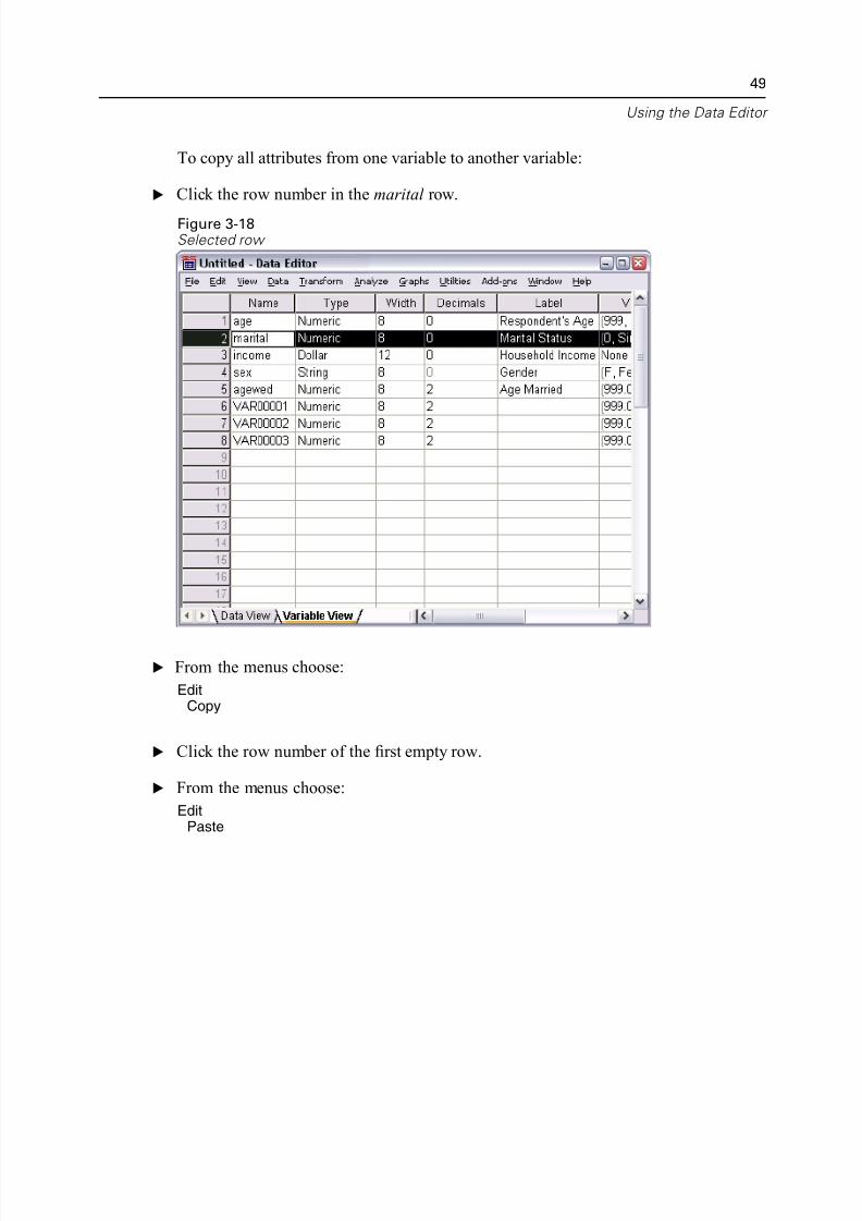
To copy all attributes from one variable to another variable:
E Click the row number in the marital row.
Figure 3-18Selected row
E From the menus choose:
EditCopy
E Click the row number of the first empty row.
E From the menus choose:
EditPaste
5/11/2018 SPSS Statistics Brief Guide 17.0 - slidepdf.com
http://slidepdf.com/reader/full/spss-statistics-brief-guide-170-55a2339b08a28 64/224
50
Chapter 3
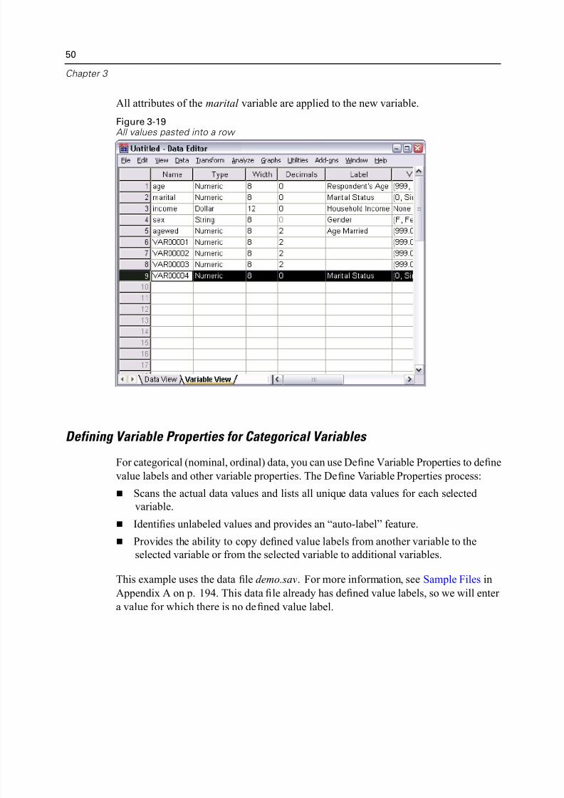
All attributes of the marital variable are applied to the new variable.
Figure 3-19All values pasted into a row
Defining Variable Properties for Categorical Variables
For categorical (nominal, ordinal) data, you can use Define Variable Properties to defi
value labels and other variable properties. The Define Variable Properties process:
Scans the actual data values and lists all unique data values for each selected
variable.
Identifies unlabeled values and provides an “auto-label” feature.
Provides the ability to copy defined value labels from another variable to the
selected variable or from the selected variable to additional variables.
This example uses the data file demo.sav. For more information, see Sample Files i
Appendix A on p. 194. This data file already has defined value labels, so we will en
a value for which there is no defined value label.
5/11/2018 SPSS Statistics Brief Guide 17.0 - slidepdf.com
http://slidepdf.com/reader/full/spss-statistics-brief-guide-170-55a2339b08a28 65/224
Using the Data Ed
E In Data View of the Data Editor, click the first data cell for the variable ownpc (you
may have to scroll to the right), and then enter 99.
E From the menus choose:
DataDefine Variable Properties...
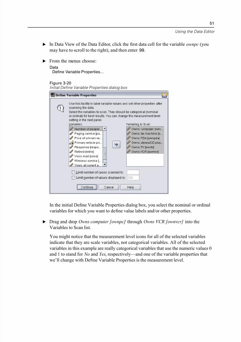
Figure 3-20Initial Define Variable Properties dialog box
In the initial Define Variable Properties dialog box, you select the nominal or ordina
variables for which you want to define value labels and/or other properties.
E Drag and drop Owns computer [ownpc] through Owns VCR [ownvcr] into the
Variables to Scan list.
You might notice that the measurement level icons for all of the selected variablesindicate that they are scale variables, not categorical variables. All of the selected
variables in this example are really categorical variables that use the numeric values
and 1 to stand for No and Yes, respectively—and one of the variable properties that
we’ll change with Define Variable Properties is the measurement level.
5/11/2018 SPSS Statistics Brief Guide 17.0 - slidepdf.com
http://slidepdf.com/reader/full/spss-statistics-brief-guide-170-55a2339b08a28 66/224
52
Chapter 3
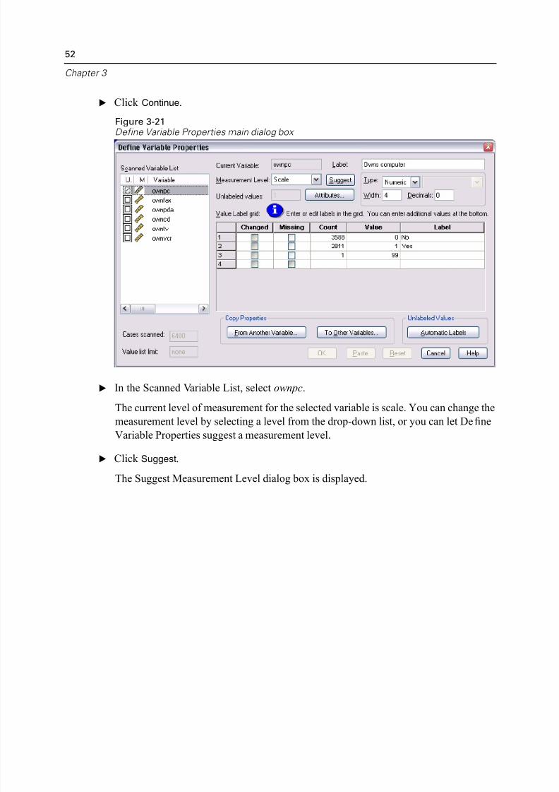
E Click Continue.
Figure 3-21Define Variable Properties main dialog box
E In the Scanned Variable List, select ownpc.
The current level of measurement for the selected variable is scale. You can change
measurement level by selecting a level from the drop-down list, or you can let Defi
Variable Properties suggest a measurement level.
E Click Suggest.
The Suggest Measurement Level dialog box is displayed.
5/11/2018 SPSS Statistics Brief Guide 17.0 - slidepdf.com
http://slidepdf.com/reader/full/spss-statistics-brief-guide-170-55a2339b08a28 67/224
Using the Data Ed
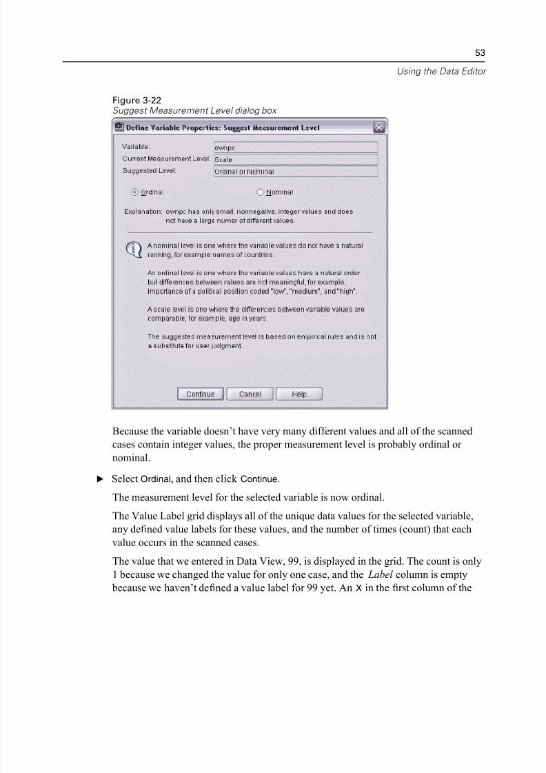
Figure 3-22Suggest Measurement Level dialog box
Because the variable doesn’t have very many different values and all of the scanned
cases contain integer values, the proper measurement level is probably ordinal or
nominal.
E Select Ordinal, and then click Continue.
The measurement level for the selected variable is now ordinal.
The Value Label grid displays all of the unique data values for the selected variable
any defined value labels for these values, and the number of times (count) that each
value occurs in the scanned cases.
The value that we entered in Data View, 99, is displayed in the grid. The count is on
1 because we changed the value for only one case, and the Label column is empty
because we haven’t defined a value label for 99 yet. An X in the first column of the
5/11/2018 SPSS Statistics Brief Guide 17.0 - slidepdf.com
http://slidepdf.com/reader/full/spss-statistics-brief-guide-170-55a2339b08a28 68/224
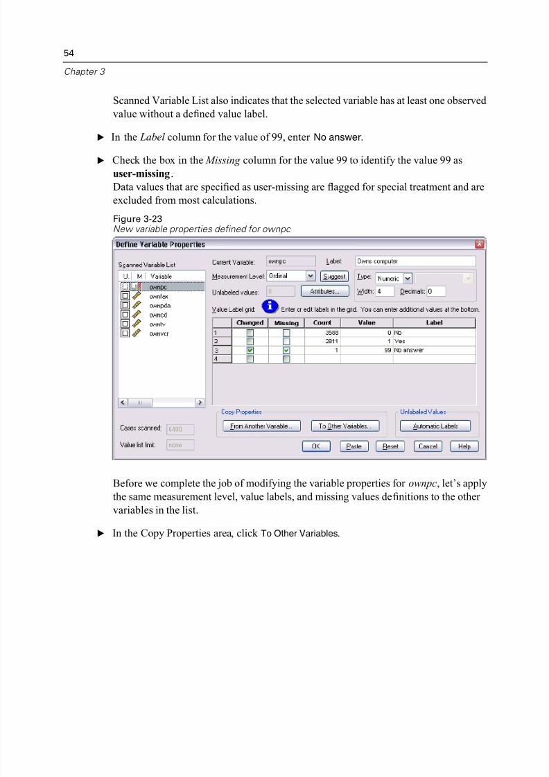
54
Chapter 3
Scanned Variable List also indicates that the selected variable has at least one observ
value without a defined value label.
E In the Label column for the value of 99, enter No answer.
E Check the box in the Missing column for the value 99 to identify the value 99 as
user-missing.
Data values that are specified as user-missing are flagged for special treatment and a
excluded from most calculations.
Figure 3-23New variable properties defined for ownpc
Before we complete the job of modifying the variable properties for ownpc, let’s ap
the same measurement level, value labels, and missing values definitions to the oth
variables in the list.
E In the Copy Properties area, click To Other Variables.
5/11/2018 SPSS Statistics Brief Guide 17.0 - slidepdf.com
http://slidepdf.com/reader/full/spss-statistics-brief-guide-170-55a2339b08a28 69/224
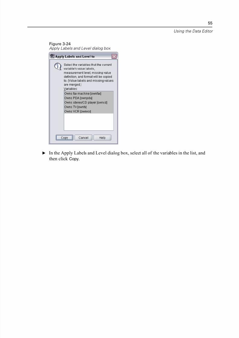
Using the Data Ed
Figure 3-24Apply Labels and Level dialog box
E In the Apply Labels and Level dialog box, select all of the variables in the list, and
then click Copy.
5/11/2018 SPSS Statistics Brief Guide 17.0 - slidepdf.com
http://slidepdf.com/reader/full/spss-statistics-brief-guide-170-55a2339b08a28 70/224
56
Chapter 3
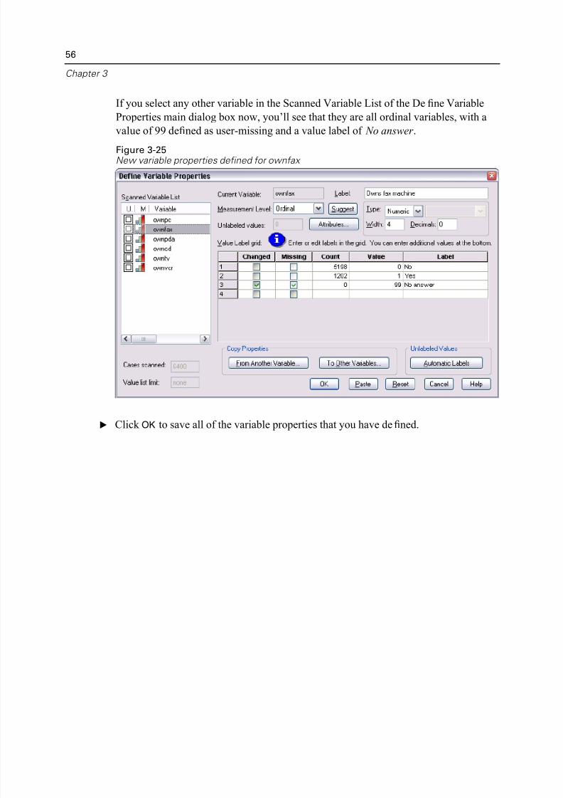
If you select any other variable in the Scanned Variable List of the Define Variable
Properties main dialog box now, you’ll see that they are all ordinal variables, with a
value of 99 defined as user-missing and a value label of No answer .
Figure 3-25New variable properties defined for ownfax
E Click OK to save all of the variable properties that you have defined.
5/11/2018 SPSS Statistics Brief Guide 17.0 - slidepdf.com
http://slidepdf.com/reader/full/spss-statistics-brief-guide-170-55a2339b08a28 71/224
Chapt
4
Working with Multiple Data Sources
Starting with version 14.0, multiple data sources can be open at the same time, mak
it easier to:
Switch back and forth between data sources.
Compare the contents of different data sources.
Copy and paste data between data sources.
Create multiple subsets of cases and/or variables for analysis.
Merge multiple data sources from various data formats (for example, spreadshe
database, text data) without saving each data source first.
57
5/11/2018 SPSS Statistics Brief Guide 17.0 - slidepdf.com
http://slidepdf.com/reader/full/spss-statistics-brief-guide-170-55a2339b08a28 72/224
58
Chapter 4
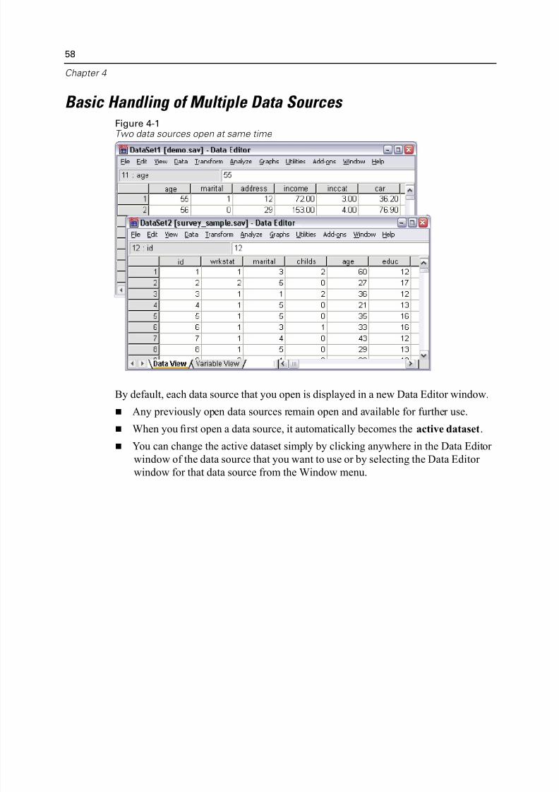
Basic Handling of Multiple Data Sources Figure 4-1
Two data sources open at same time
By default, each data source that you open is displayed in a new Data Editor window
Any previously open data sources remain open and available for further use. When you first open a data source, it automatically becomes the active dataset
You can change the active dataset simply by clicking anywhere in the Data Edit
window of the data source that you want to use or by selecting the Data Editor
window for that data source from the Window menu.
5/11/2018 SPSS Statistics Brief Guide 17.0 - slidepdf.com
http://slidepdf.com/reader/full/spss-statistics-brief-guide-170-55a2339b08a28 73/224
Working with Multiple Data Sour
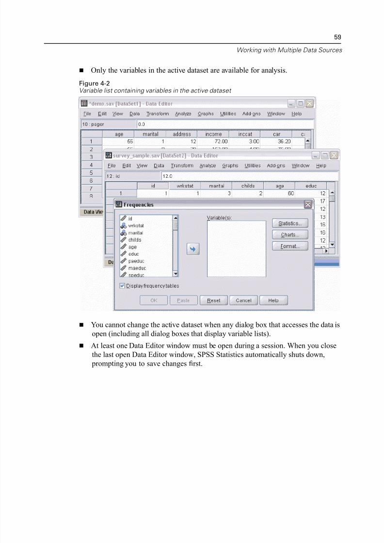
Only the variables in the active dataset are available for analysis.
Figure 4-2Variable list containing variables in the active dataset
You cannot change the active dataset when any dialog box that accesses the dat
open (including all dialog boxes that display variable lists).
At least one Data Editor window must be open during a session. When you clo
the last open Data Editor window, SPSS Statistics automatically shuts down,
prompting you to save changes first.
5/11/2018 SPSS Statistics Brief Guide 17.0 - slidepdf.com
http://slidepdf.com/reader/full/spss-statistics-brief-guide-170-55a2339b08a28 74/224
60
Chapter 4
Working with Multiple Datasets in Command Syntax
If you use command syntax to open data sources (for example, GET FILE, GET
DATA), you need to use the DATASET NAME command to name each dataset explici
in order to have more than one data source open at the same time.
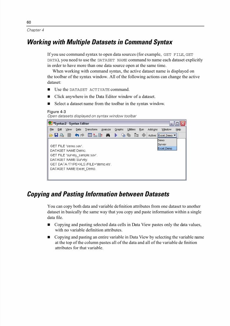
When working with command syntax, the active dataset name is displayed on
the toolbar of the syntax window. All of the following actions can change the activ
dataset:
Use the DATASET ACTIVATE command.
Click anywhere in the Data Editor window of a dataset.
Select a dataset name from the toolbar in the syntax window.
Figure 4-3Open datasets displayed on syntax window toolbar
Copying and Pasting Information between Datasets
You can copy both data and variable definition attributes from one dataset to anothe
dataset in basically the same way that you copy and paste information within a sing
data file.
Copying and pasting selected data cells in Data View pastes only the data value
with no variable definition attributes.
Copying and pasting an entire variable in Data View by selecting the variable na
at the top of the column pastes all of the data and all of the variable definition
attributes for that variable.
5/11/2018 SPSS Statistics Brief Guide 17.0 - slidepdf.com
http://slidepdf.com/reader/full/spss-statistics-brief-guide-170-55a2339b08a28 75/224
Working with Multiple Data Sour
Copying and pasting variable definition attributes or entire variables in Variable
View pastes the selected attributes (or the entire variable definition) but does no
paste any data values.
Renaming Datasets
When you open a data source through the menus and dialog boxes, each data source
is automatically assigned a dataset name of DataSetn, where n is a sequential intege
value, and when you open a data source using command syntax, no dataset name is
assigned unless you explicitly specify one with DATASET NAME. To provide more
descriptive dataset names:
E From the menus in the Data Editor window for the dataset whose name you want
to change choose:
FileRename Dataset...
E Enter a new dataset name that conforms to variable naming rules.
Suppressing Multiple Datasets
If you prefer to have only one dataset available at a time and want to suppress themultiple dataset feature:
E From the menus choose:
EditOptions...
E Click the General tab.
Select (check) Open only one dataset at a time.
5/11/2018 SPSS Statistics Brief Guide 17.0 - slidepdf.com
http://slidepdf.com/reader/full/spss-statistics-brief-guide-170-55a2339b08a28 76/224
Chapt
5
Examining Summary Statistics for Individual Variables
This chapter discusses simple summary measures and how the level of measuremen
a variable influences the types of statistics that should be used. We will use the data
demo.sav. For more information, see Sample Files in Appendix A on p. 194.
Level of Measurement
Different summary measures are appropriate for different types of data, depending o
the level of measurement:
Categorical. Data with a limited number of distinct values or categories (for exampl
gender or marital status). Also referred to as qualitative data. Categorical variable
can be string (alphanumeric) data or numeric variables that use numeric codes torepresent categories (for example, 0 = Unmarried and 1 = Married ). There are two
basic types of categorical data:
Nominal. Categorical data where there is no inherent order to the categories. Fo
example, a job category of sales is not higher or lower than a job category of
marketing or research.
Ordinal. Categorical data where there is a meaningful order of categories, but
there is not a measurable distance between categories. For example, there is an
order to the values high, medium, and low, but the “distance” between the value
cannot be calculated.
Scale. Data measured on an interval or ratio scale, where the data values indicate bo
the order of values and the distance between values. For example, a salary of $72,1
is higher than a salary of $52,398, and the distance between the two values is $19,79
Also referred to as quantitative or continuous data.
62
5/11/2018 SPSS Statistics Brief Guide 17.0 - slidepdf.com
http://slidepdf.com/reader/full/spss-statistics-brief-guide-170-55a2339b08a28 77/224
Examining Summary Statistics for Individual Variab
Summary Measures for Categorical Data For categorical data, the most typical summary measure is the number or percentag
cases in each category. The mode is the category with the greatest number of cases
For ordinal data, the median (the value at which half of the cases fall above and belo
may also be a useful summary measure if there is a large number of categories.
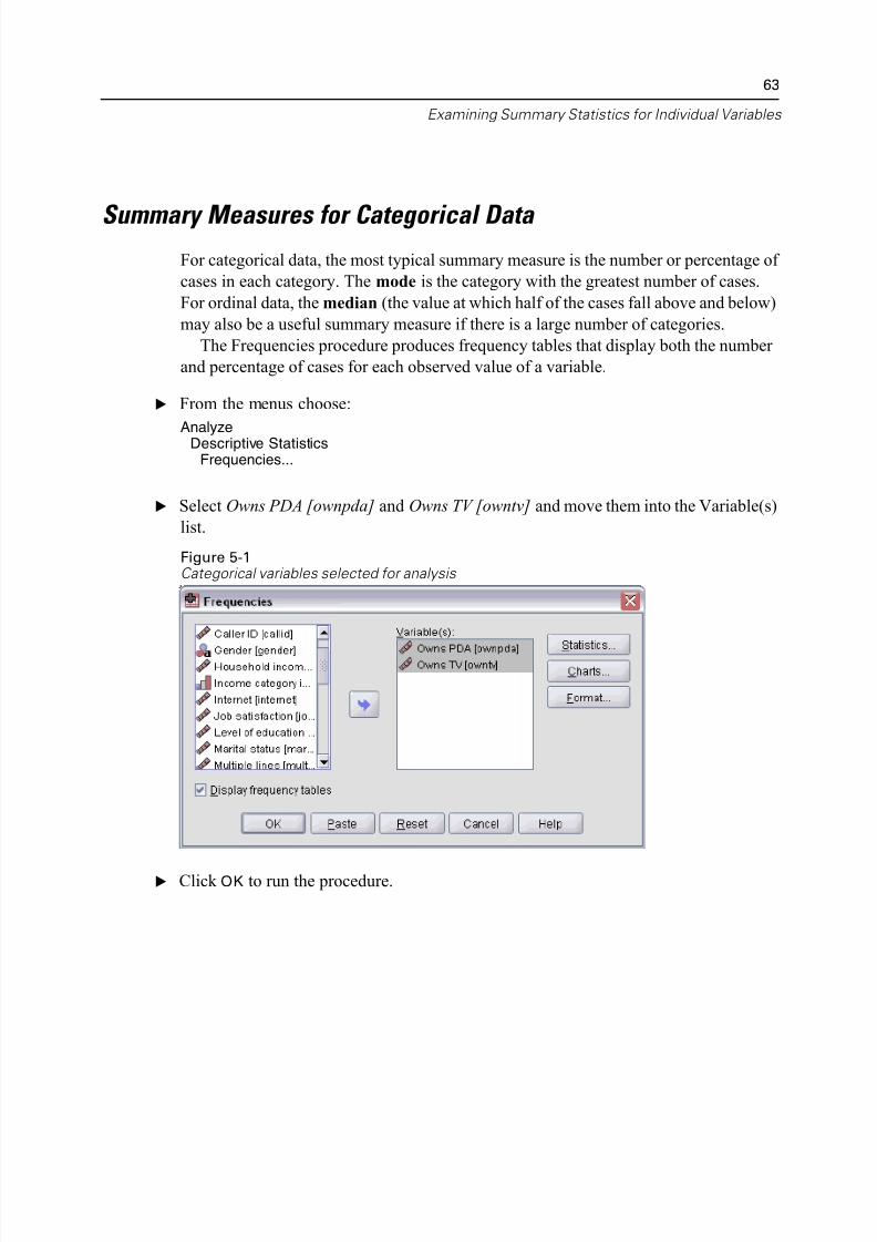
The Frequencies procedure produces frequency tables that display both the numb
and percentage of cases for each observed value of a variable.
E From the menus choose:
AnalyzeDescriptive StatisticsFrequencies...
E Select Owns PDA [ownpda] and Owns TV [owntv] and move them into the Variable
list.
Figure 5-1Categorical variables selected for analysis
E Click OK to run the procedure.
5/11/2018 SPSS Statistics Brief Guide 17.0 - slidepdf.com
http://slidepdf.com/reader/full/spss-statistics-brief-guide-170-55a2339b08a28 78/224
64
Chapter 5
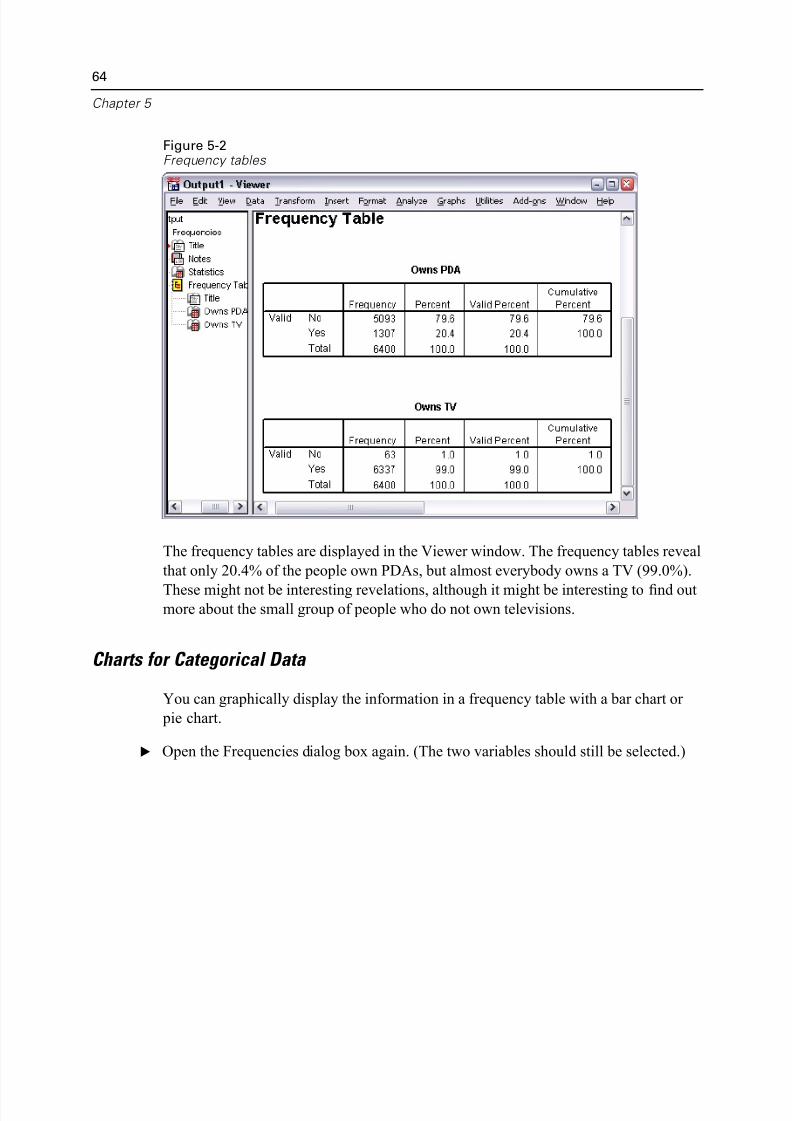
Figure 5-2Frequency tables
The frequency tables are displayed in the Viewer window. The frequency tables rev
that only 20.4% of the people own PDAs, but almost everybody owns a TV (99.0%
These might not be interesting revelations, although it might be interesting to find omore about the small group of people who do not own televisions.
Charts for Categorical Data
You can graphically display the information in a frequency table with a bar chart or
pie chart.
E Open the Frequencies dialog box again. (The two variables should still be selected.)
5/11/2018 SPSS Statistics Brief Guide 17.0 - slidepdf.com
http://slidepdf.com/reader/full/spss-statistics-brief-guide-170-55a2339b08a28 79/224
Examining Summary Statistics for Individual Variab
You can use the Dialog Recall button on the toolbar to quickly return to recently use
procedures.
Figure 5-3Dialog Recall button
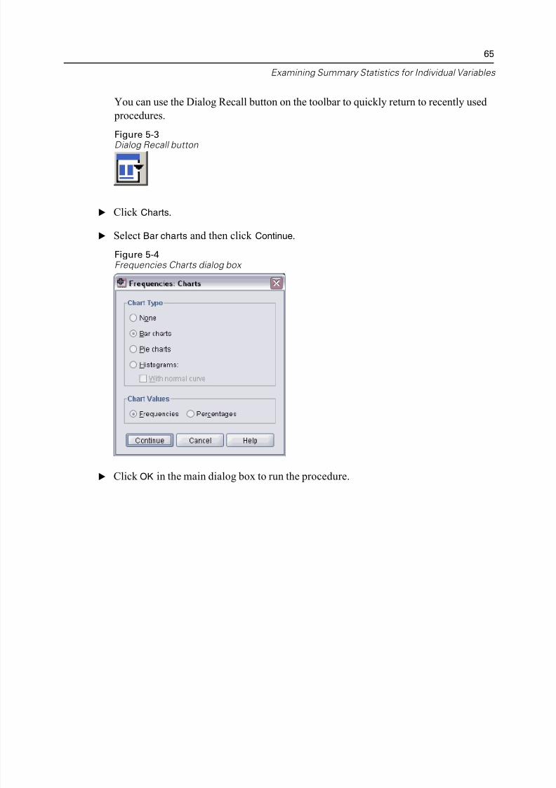
E Click Charts.
E Select Bar charts and then click Continue.
Figure 5-4Frequencies Charts dialog box
E Click OK in the main dialog box to run the procedure.
5/11/2018 SPSS Statistics Brief Guide 17.0 - slidepdf.com
http://slidepdf.com/reader/full/spss-statistics-brief-guide-170-55a2339b08a28 80/224
66
Chapter 5
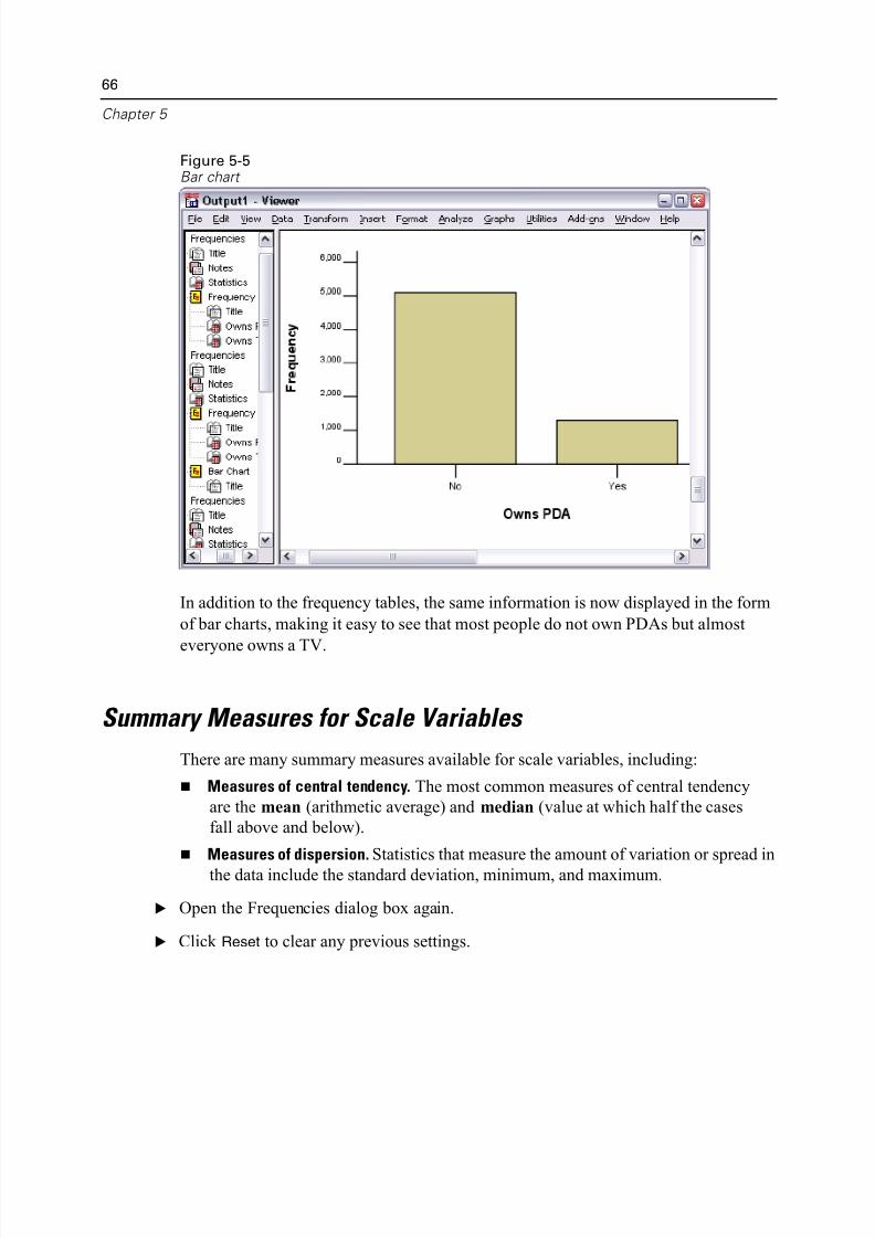
Figure 5-5Bar chart
In addition to the frequency tables, the same information is now displayed in the fo
of bar charts, making it easy to see that most people do not own PDAs but almost
everyone owns a TV.
Summary Measures for Scale Variables
There are many summary measures available for scale variables, including:
Measures of central tendency. The most common measures of central tendency
are the mean (arithmetic average) and median (value at which half the cases
fall above and below).
Measures of dispersion. Statistics that measure the amount of variation or spread
the data include the standard deviation, minimum, and maximum.
E Open the Frequencies dialog box again.
E Click Reset to clear any previous settings.
5/11/2018 SPSS Statistics Brief Guide 17.0 - slidepdf.com
http://slidepdf.com/reader/full/spss-statistics-brief-guide-170-55a2339b08a28 81/224
Examining Summary Statistics for Individual Variab
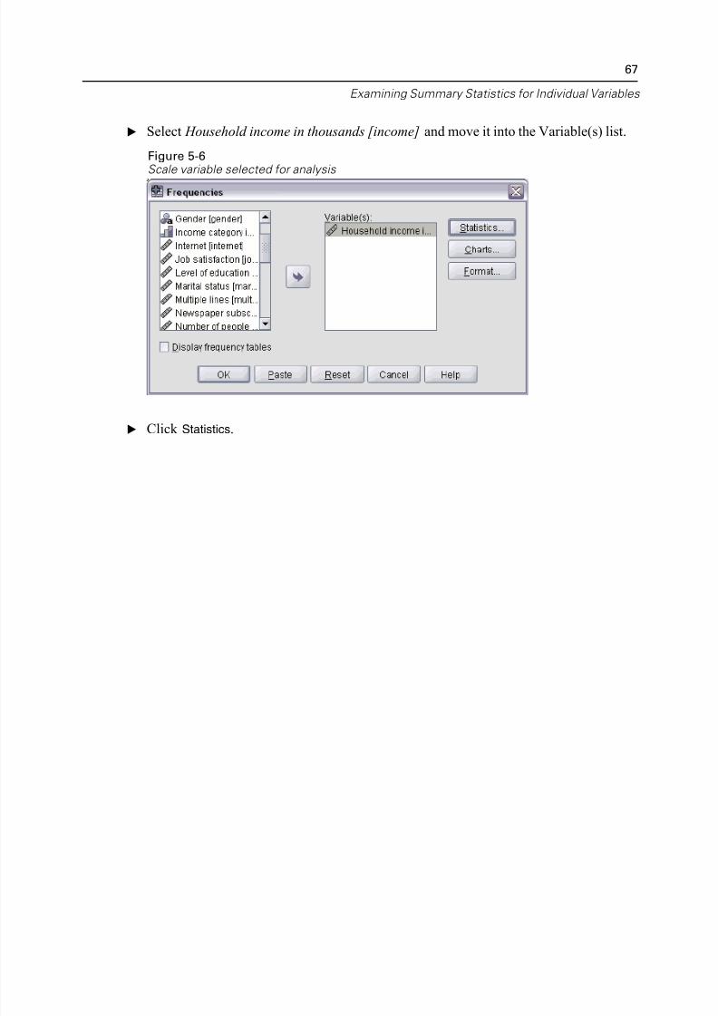
E Select Household income in thousands [income] and move it into the Variable(s) lis
Figure 5-6Scale variable selected for analysis
E Click Statistics.
5/11/2018 SPSS Statistics Brief Guide 17.0 - slidepdf.com
http://slidepdf.com/reader/full/spss-statistics-brief-guide-170-55a2339b08a28 82/224
68
Chapter 5
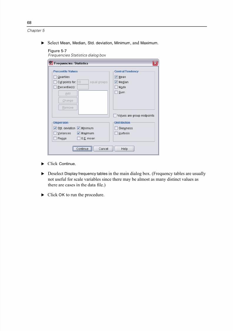
E Select Mean, Median, Std. deviation, Minimum, and Maximum.
Figure 5-7Frequencies Statistics dialog box
E Click Continue.
E Deselect Display frequency tables in the main dialog box. (Frequency tables are usuanot useful for scale variables since there may be almost as many distinct values as
there are cases in the data file.)
E Click OK to run the procedure.
5/11/2018 SPSS Statistics Brief Guide 17.0 - slidepdf.com
http://slidepdf.com/reader/full/spss-statistics-brief-guide-170-55a2339b08a28 83/224
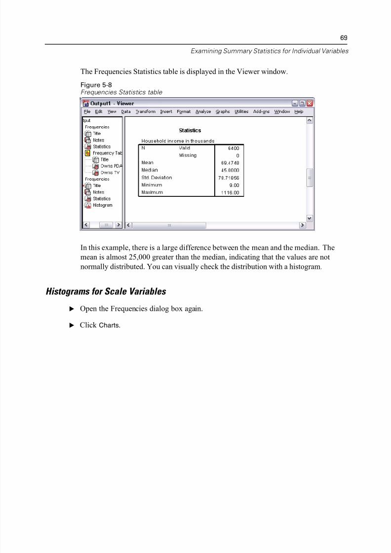
Examining Summary Statistics for Individual Variab
The Frequencies Statistics table is displayed in the Viewer window.
Figure 5-8Frequencies Statistics table
In this example, there is a large difference between the mean and the median. The
mean is almost 25,000 greater than the median, indicating that the values are not
normally distributed. You can visually check the distribution with a histogram.
Histograms for Scale Variables
E Open the Frequencies dialog box again.
E Click Charts.
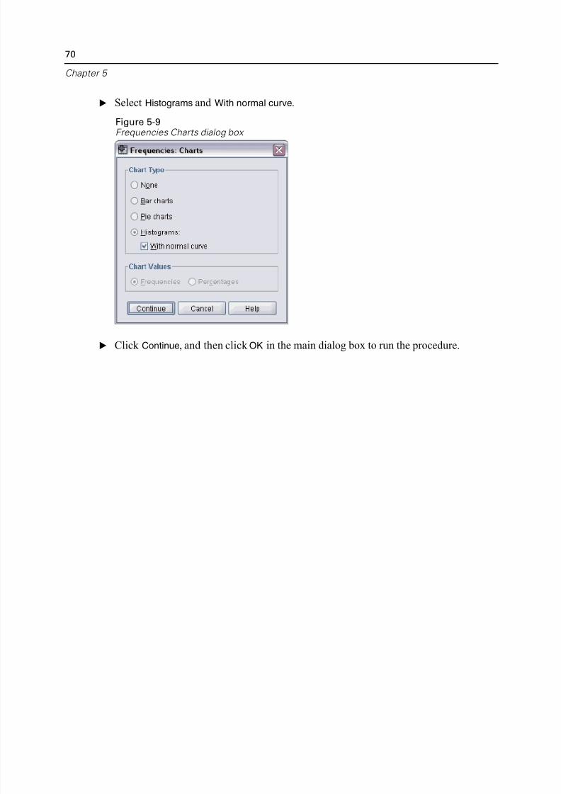
5/11/2018 SPSS Statistics Brief Guide 17.0 - slidepdf.com
http://slidepdf.com/reader/full/spss-statistics-brief-guide-170-55a2339b08a28 84/224
70
Chapter 5
E Select Histograms and With normal curve.
Figure 5-9Frequencies Charts dialog box
E Click Continue, and then click OK in the main dialog box to run the procedure.
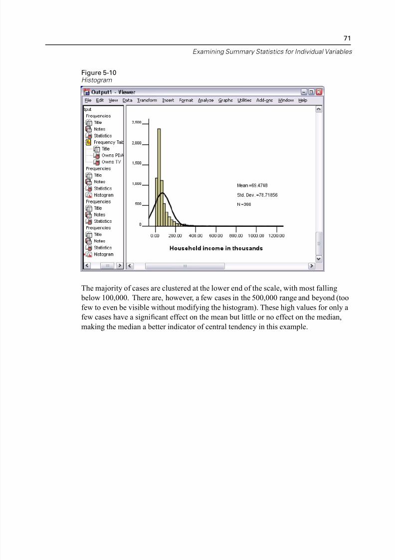
5/11/2018 SPSS Statistics Brief Guide 17.0 - slidepdf.com
http://slidepdf.com/reader/full/spss-statistics-brief-guide-170-55a2339b08a28 85/224
Examining Summary Statistics for Individual Variab
Figure 5-10Histogram
The majority of cases are clustered at the lower end of the scale, with most falling
below 100,000. There are, however, a few cases in the 500,000 range and beyond (t
few to even be visible without modifying the histogram). These high values for onl
few cases have a significant effect on the mean but little or no effect on the median
making the median a better indicator of central tendency in this example.
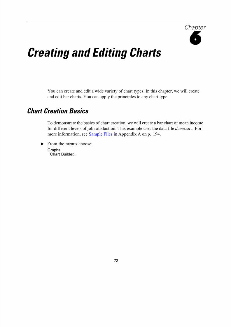
5/11/2018 SPSS Statistics Brief Guide 17.0 - slidepdf.com
http://slidepdf.com/reader/full/spss-statistics-brief-guide-170-55a2339b08a28 86/224
Chapt
6
Creating and Editing Charts
You can create and edit a wide variety of chart types. In this chapter, we will create
and edit bar charts. You can apply the principles to any chart type.
Chart Creation Basics To demonstrate the basics of chart creation, we will create a bar chart of mean incom
for different levels of job satisfaction. This example uses the data file demo.sav. Fo
more information, see Sample Files in Appendix A on p. 194.
E From the menus choose:
GraphsChart Builder...
72
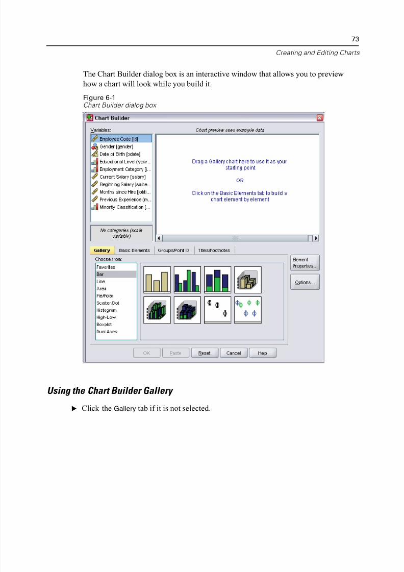
5/11/2018 SPSS Statistics Brief Guide 17.0 - slidepdf.com
http://slidepdf.com/reader/full/spss-statistics-brief-guide-170-55a2339b08a28 87/224
Creating and Editing Ch
The Chart Builder dialog box is an interactive window that allows you to preview
how a chart will look while you build it.
Figure 6-1Chart Builder dialog box
Using the Chart Builder Gallery
E Click the Gallery tab if it is not selected.

5/11/2018 SPSS Statistics Brief Guide 17.0 - slidepdf.com
http://slidepdf.com/reader/full/spss-statistics-brief-guide-170-55a2339b08a28 88/224
74
Chapter 6
The Gallery includes many different predefined charts, which are organized by char
type. The Basic Elements tab also provides basic elements (such as axes and graph
elements) for creating charts from scratch, but it’s easier to use the Gallery.
E Click Bar if it is not selected.
Icons representing the available bar charts in the Gallery appear in the dialog box. T
pictures should provide enough information to identify the specific chart type. If yo
need more information, you can also display a ToolTip description of the chart by
pausing your cursor over an icon.
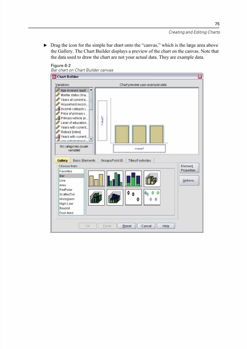
5/11/2018 SPSS Statistics Brief Guide 17.0 - slidepdf.com
http://slidepdf.com/reader/full/spss-statistics-brief-guide-170-55a2339b08a28 89/224
Creating and Editing Ch
E Drag the icon for the simple bar chart onto the “canvas,” which is the large area abo
the Gallery. The Chart Builder displays a preview of the chart on the canvas. Note t
the data used to draw the chart are not your actual data. They are example data.
Figure 6-2Bar chart on Chart Builder canvas
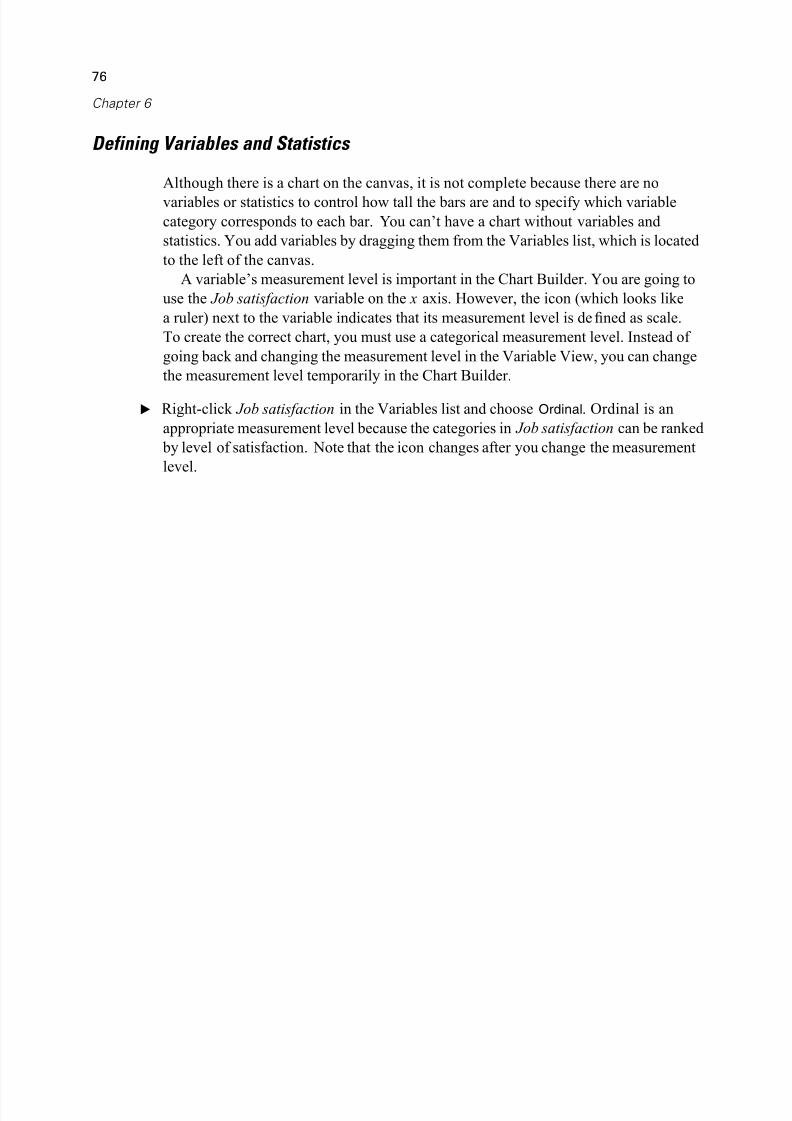
5/11/2018 SPSS Statistics Brief Guide 17.0 - slidepdf.com
http://slidepdf.com/reader/full/spss-statistics-brief-guide-170-55a2339b08a28 90/224
76
Chapter 6
Defining Variables and Statistics
Although there is a chart on the canvas, it is not complete because there are no
variables or statistics to control how tall the bars are and to specify which variable
category corresponds to each bar. You can’t have a chart without variables and
statistics. You add variables by dragging them from the Variables list, which is loca
to the left of the canvas.
A variable’s measurement level is important in the Chart Builder. You are going
use the Job satisfaction variable on the x axis. However, the icon (which looks like
a ruler) next to the variable indicates that its measurement level is defined as scale.
To create the correct chart, you must use a categorical measurement level. Instead o
going back and changing the measurement level in the Variable View, you can chan
the measurement level temporarily in the Chart Builder.
E Right-click Job satisfaction in the Variables list and choose Ordinal. Ordinal is an
appropriate measurement level because the categories in Job satisfaction can be ran
by level of satisfaction. Note that the icon changes after you change the measureme
level.
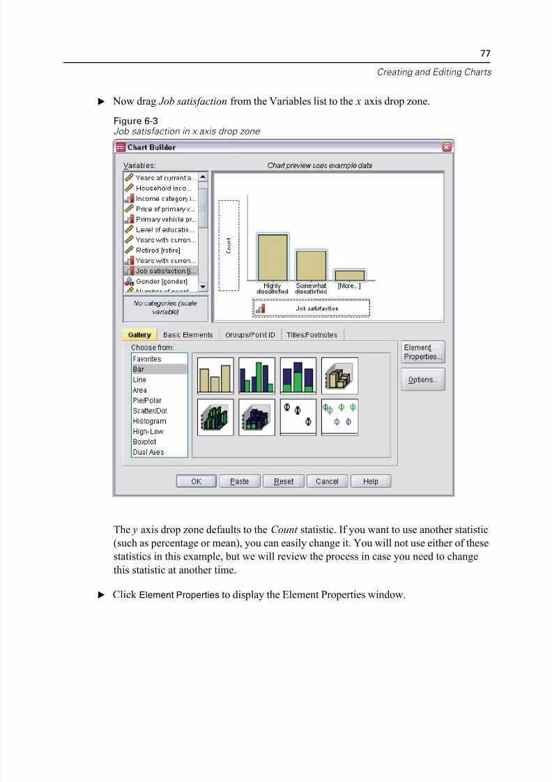
5/11/2018 SPSS Statistics Brief Guide 17.0 - slidepdf.com
http://slidepdf.com/reader/full/spss-statistics-brief-guide-170-55a2339b08a28 91/224
Creating and Editing Ch
E Now drag Job satisfaction from the Variables list to the x axis drop zone.
Figure 6-3Job satisfaction in x axis drop zone
The y axis drop zone defaults to the Count statistic. If you want to use another stati
(such as percentage or mean), you can easily change it. You will not use either of thstatistics in this example, but we will review the process in case you need to chang
this statistic at another time.
E Click Element Properties to display the Element Properties window.
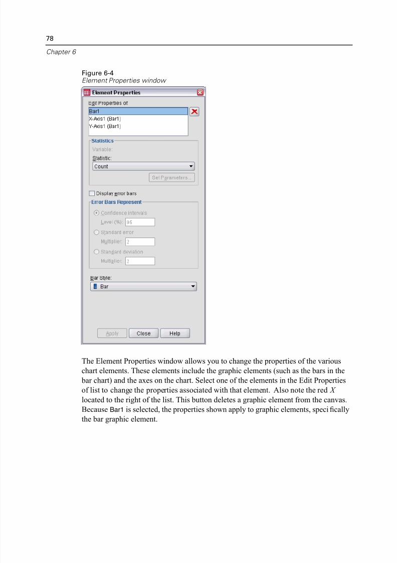
5/11/2018 SPSS Statistics Brief Guide 17.0 - slidepdf.com
http://slidepdf.com/reader/full/spss-statistics-brief-guide-170-55a2339b08a28 92/224
78
Chapter 6
Figure 6-4Element Properties window
The Element Properties window allows you to change the properties of the various
chart elements. These elements include the graphic elements (such as the bars in th
bar chart) and the axes on the chart. Select one of the elements in the Edit Propertie
of list to change the properties associated with that element. Also note the red X located to the right of the list. This button deletes a graphic element from the canva
Because Bar1 is selected, the properties shown apply to graphic elements, specifical
the bar graphic element.
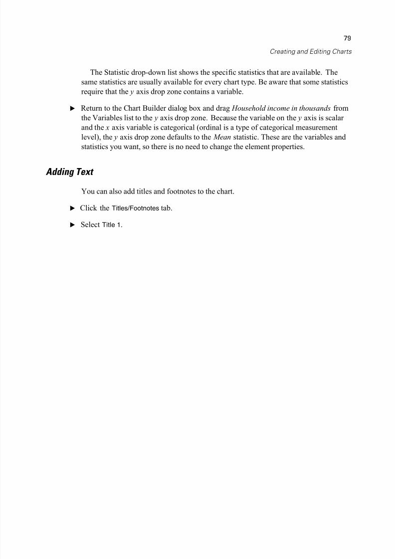
5/11/2018 SPSS Statistics Brief Guide 17.0 - slidepdf.com
http://slidepdf.com/reader/full/spss-statistics-brief-guide-170-55a2339b08a28 93/224
Creating and Editing Ch
The Statistic drop-down list shows the specific statistics that are available. The
same statistics are usually available for every chart type. Be aware that some statist
require that the y axis drop zone contains a variable.
E Return to the Chart Builder dialog box and drag Household income in thousands fro
the Variables list to the y axis drop zone. Because the variable on the y axis is scala
and the x axis variable is categorical (ordinal is a type of categorical measurement
level), the y axis drop zone defaults to the Mean statistic. These are the variables an
statistics you want, so there is no need to change the element properties.
Adding Text
You can also add titles and footnotes to the chart.
E Click the Titles/Footnotes tab.
E Select Title 1.
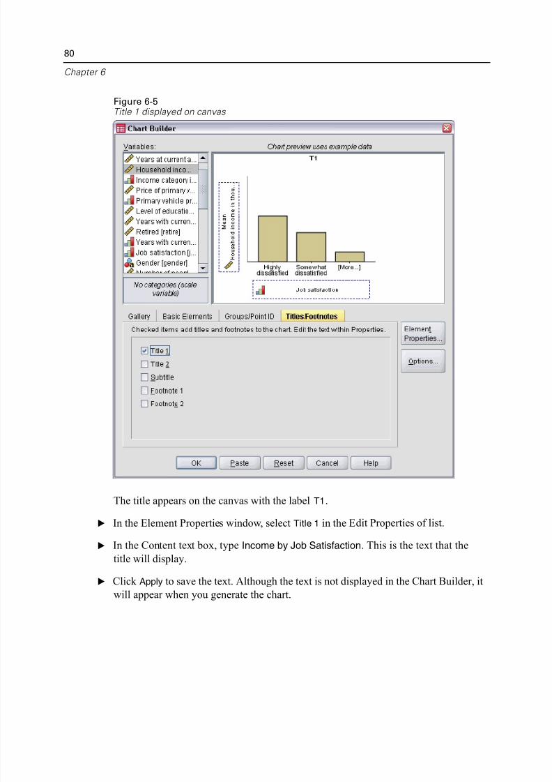
5/11/2018 SPSS Statistics Brief Guide 17.0 - slidepdf.com
http://slidepdf.com/reader/full/spss-statistics-brief-guide-170-55a2339b08a28 94/224
80
Chapter 6
Figure 6-5Title 1 displayed on canvas
The title appears on the canvas with the label T1.
E In the Element Properties window, select Title 1 in the Edit Properties of list.
E In the Content text box, type Income by Job Satisfaction. This is the text that thetitle will display.
E Click Apply to save the text. Although the text is not displayed in the Chart Builder,
will appear when you generate the chart.
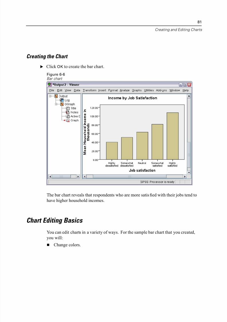
5/11/2018 SPSS Statistics Brief Guide 17.0 - slidepdf.com
http://slidepdf.com/reader/full/spss-statistics-brief-guide-170-55a2339b08a28 95/224
Creating and Editing Ch
Creating the Chart
E Click OK to create the bar chart.
Figure 6-6Bar chart
The bar chart reveals that respondents who are more satisfied with their jobs tend to
have higher household incomes.
Chart Editing Basics
You can edit charts in a variety of ways. For the sample bar chart that you created,
you will:
Change colors.
5/11/2018 SPSS Statistics Brief Guide 17.0 - slidepdf.com
http://slidepdf.com/reader/full/spss-statistics-brief-guide-170-55a2339b08a28 96/224
82
Chapter 6
Format numbers in tick labels.
Edit text.
Display data value labels. Use chart templates.
To edit the chart, open it in the Chart Editor.
E Double-click the bar chart to open it in the Chart Editor.
Figure 6-7Bar chart in the Chart Editor
Selecting Chart Elements
To edit a chart element, you first select it.
E Click any one of the bars. The rectangles around the bars indicate that they are select
5/11/2018 SPSS Statistics Brief Guide 17.0 - slidepdf.com
http://slidepdf.com/reader/full/spss-statistics-brief-guide-170-55a2339b08a28 97/224
Creating and Editing Ch
There are general rules for selecting elements in simple charts:
When no graphic elements are selected, click any graphic element to select all
graphic elements. When all graphic elements are selected, click a graphic element to select only th
graphic element. You can select a different graphic element by clicking it. To
select multiple graphic elements, click each element while pressing the Ctrl key
E To deselect all elements, press the Esc key.
E Click any bar to select all of the bars again.
Using the Properties Window E From the Chart Editor menus choose:
EditProperties
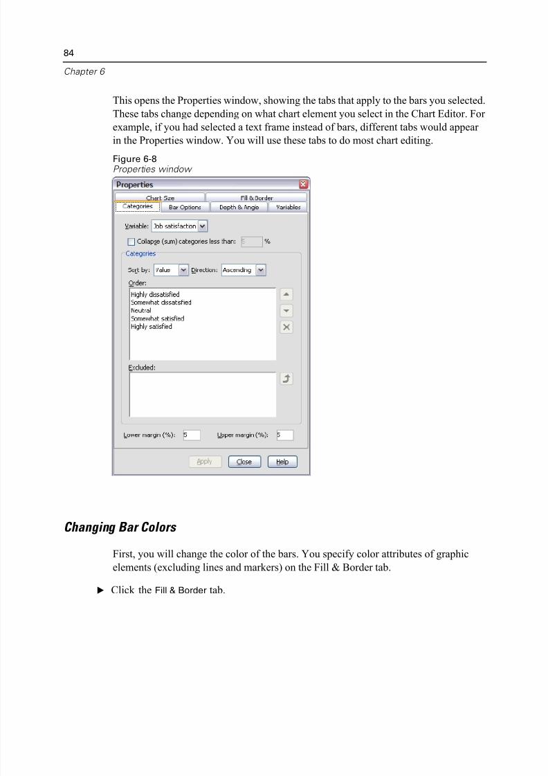
5/11/2018 SPSS Statistics Brief Guide 17.0 - slidepdf.com
http://slidepdf.com/reader/full/spss-statistics-brief-guide-170-55a2339b08a28 98/224
84
Chapter 6
This opens the Properties window, showing the tabs that apply to the bars you select
These tabs change depending on what chart element you select in the Chart Editor. F
example, if you had selected a text frame instead of bars, different tabs would appe
in the Properties window. You will use these tabs to do most chart editing.
Figure 6-8Properties window
Changing Bar Colors
First, you will change the color of the bars. You specify color attributes of graphic
elements (excluding lines and markers) on the Fill & Border tab.
E Click the Fill & Border tab.
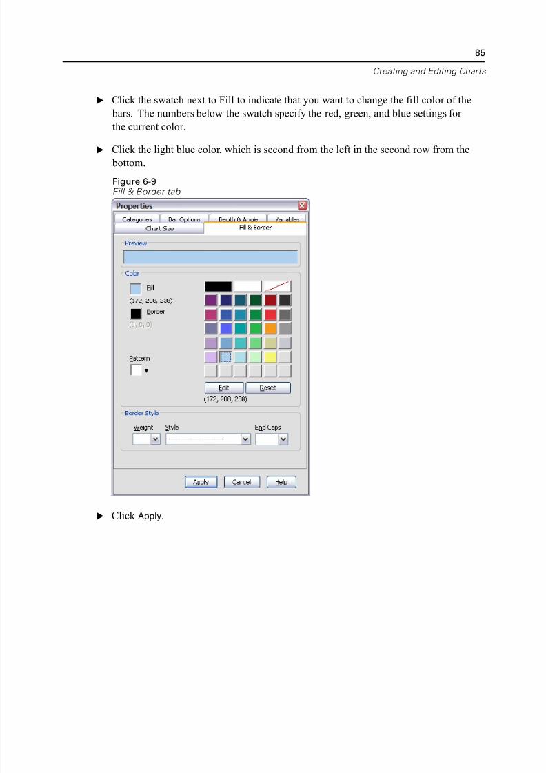
5/11/2018 SPSS Statistics Brief Guide 17.0 - slidepdf.com
http://slidepdf.com/reader/full/spss-statistics-brief-guide-170-55a2339b08a28 99/224
Creating and Editing Ch
E Click the swatch next to Fill to indicate that you want to change the fill color of the
bars. The numbers below the swatch specify the red, green, and blue settings for
the current color.
E Click the light blue color, which is second from the left in the second row from the
bottom.
Figure 6-9Fill & Border tab
E Click Apply.
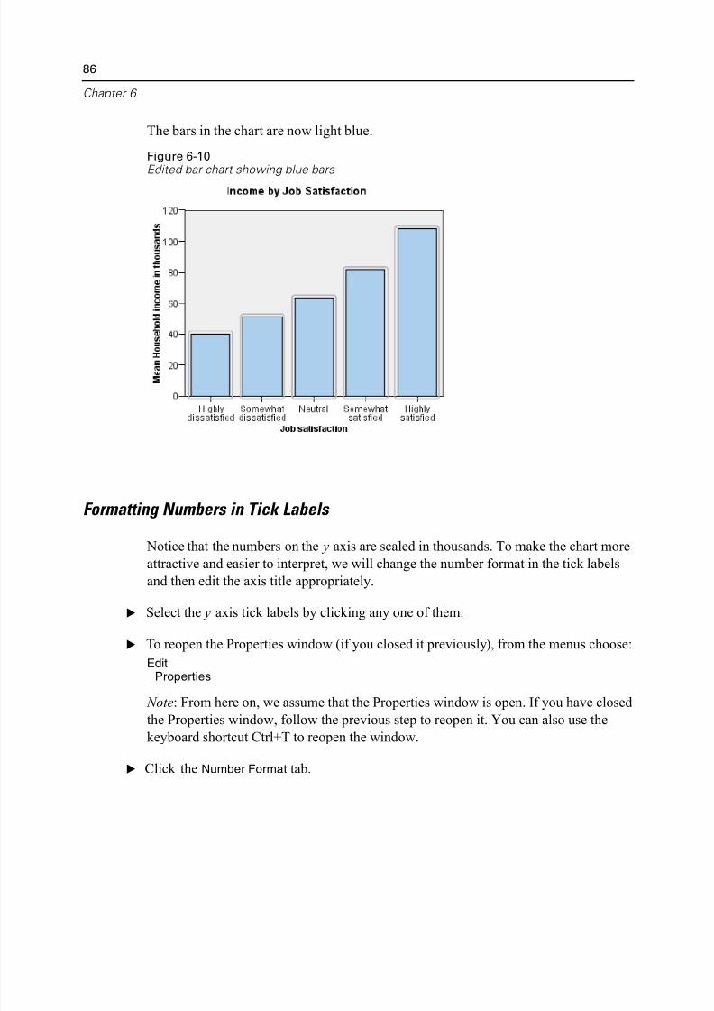
5/11/2018 SPSS Statistics Brief Guide 17.0 - slidepdf.com
http://slidepdf.com/reader/full/spss-statistics-brief-guide-170-55a2339b08a28 100/224
86
Chapter 6
The bars in the chart are now light blue.
Figure 6-10Edited bar chart showing blue bars
Formatting Numbers in Tick Labels
Notice that the numbers on the y axis are scaled in thousands. To make the chart mo
attractive and easier to interpret, we will change the number format in the tick label
and then edit the axis title appropriately.
E Select the y axis tick labels by clicking any one of them.
E To reopen the Properties window (if you closed it previously), from the menus choo
EditProperties
Note: From here on, we assume that the Properties window is open. If you have clothe Properties window, follow the previous step to reopen it. You can also use the
keyboard shortcut Ctrl+T to reopen the window.
E Click the Number Format tab.
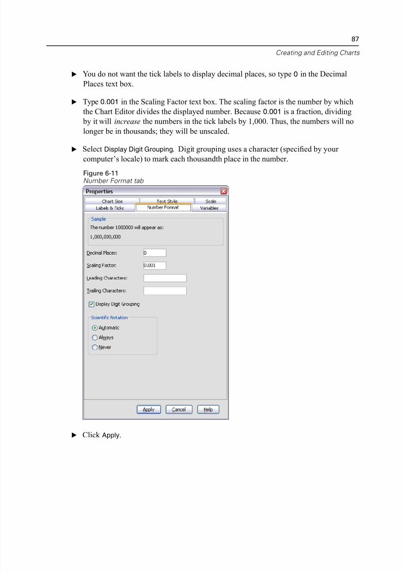
5/11/2018 SPSS Statistics Brief Guide 17.0 - slidepdf.com
http://slidepdf.com/reader/full/spss-statistics-brief-guide-170-55a2339b08a28 101/224
Creating and Editing Ch
E You do not want the tick labels to display decimal places, so type 0 in the Decimal
Places text box.
E Type 0.001 in the Scaling Factor text box. The scaling factor is the number by whicthe Chart Editor divides the displayed number. Because 0.001 is a fraction, dividin
by it will increase the numbers in the tick labels by 1,000. Thus, the numbers will n
longer be in thousands; they will be unscaled.
E Select Display Digit Grouping. Digit grouping uses a character (specified by your
computer’s locale) to mark each thousandth place in the number.
Figure 6-11Number Format tab
E Click Apply.
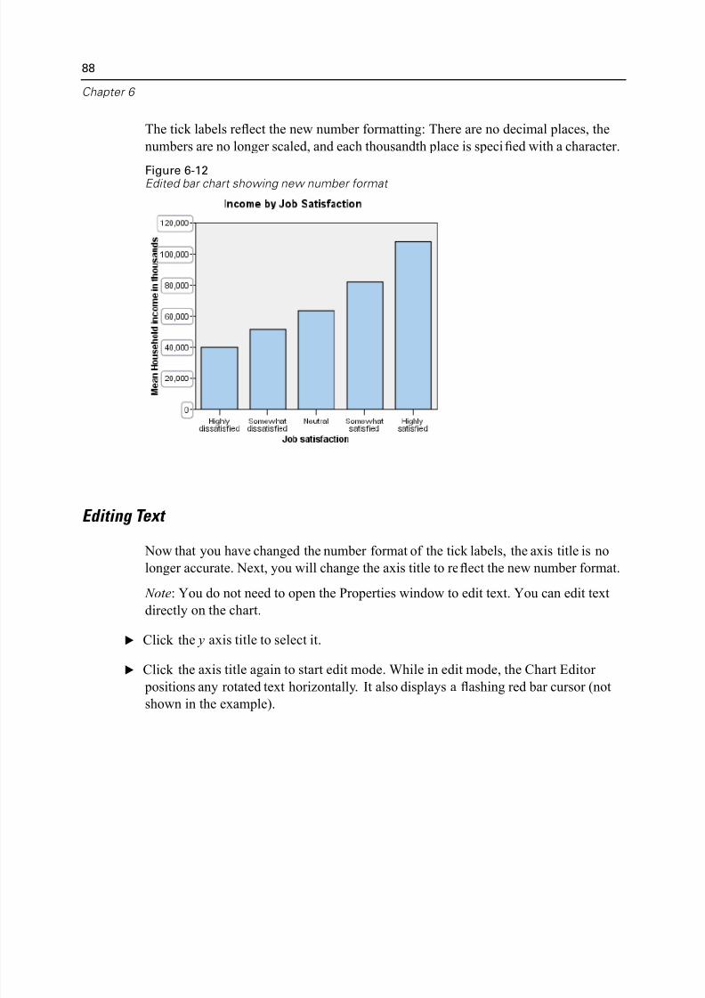
5/11/2018 SPSS Statistics Brief Guide 17.0 - slidepdf.com
http://slidepdf.com/reader/full/spss-statistics-brief-guide-170-55a2339b08a28 102/224
88
Chapter 6
The tick labels reflect the new number formatting: There are no decimal places, the
numbers are no longer scaled, and each thousandth place is specified with a charact
Figure 6-12Edited bar chart showing new number format
Editing T ext Now that you have changed the number format of the tick labels, the axis title is no
longer accurate. Next, you will change the axis title to reflect the new number form
Note: You do not need to open the Properties window to edit text. You can edit tex
directly on the chart.
E Click the y axis title to select it.
E Click the axis title again to start edit mode. While in edit mode, the Chart Editor
positions any rotated text horizontally. It also displays a flashing red bar cursor (no
shown in the example).
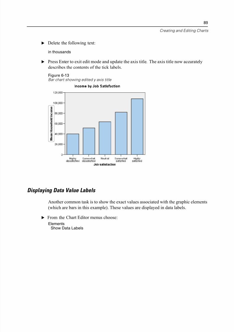
5/11/2018 SPSS Statistics Brief Guide 17.0 - slidepdf.com
http://slidepdf.com/reader/full/spss-statistics-brief-guide-170-55a2339b08a28 103/224
Creating and Editing Ch
E Delete the following text:
in thousands
E Press Enter to exit edit mode and update the axis title. The axis title now accurately
describes the contents of the tick labels.
Figure 6-13Bar chart showing edited y axis title
Displaying Data Value Labels
Another common task is to show the exact values associated with the graphic eleme
(which ar e bars in this example). These values are displayed in data labels.
E From the Chart Editor menus choose:
ElementsShow Data Labels
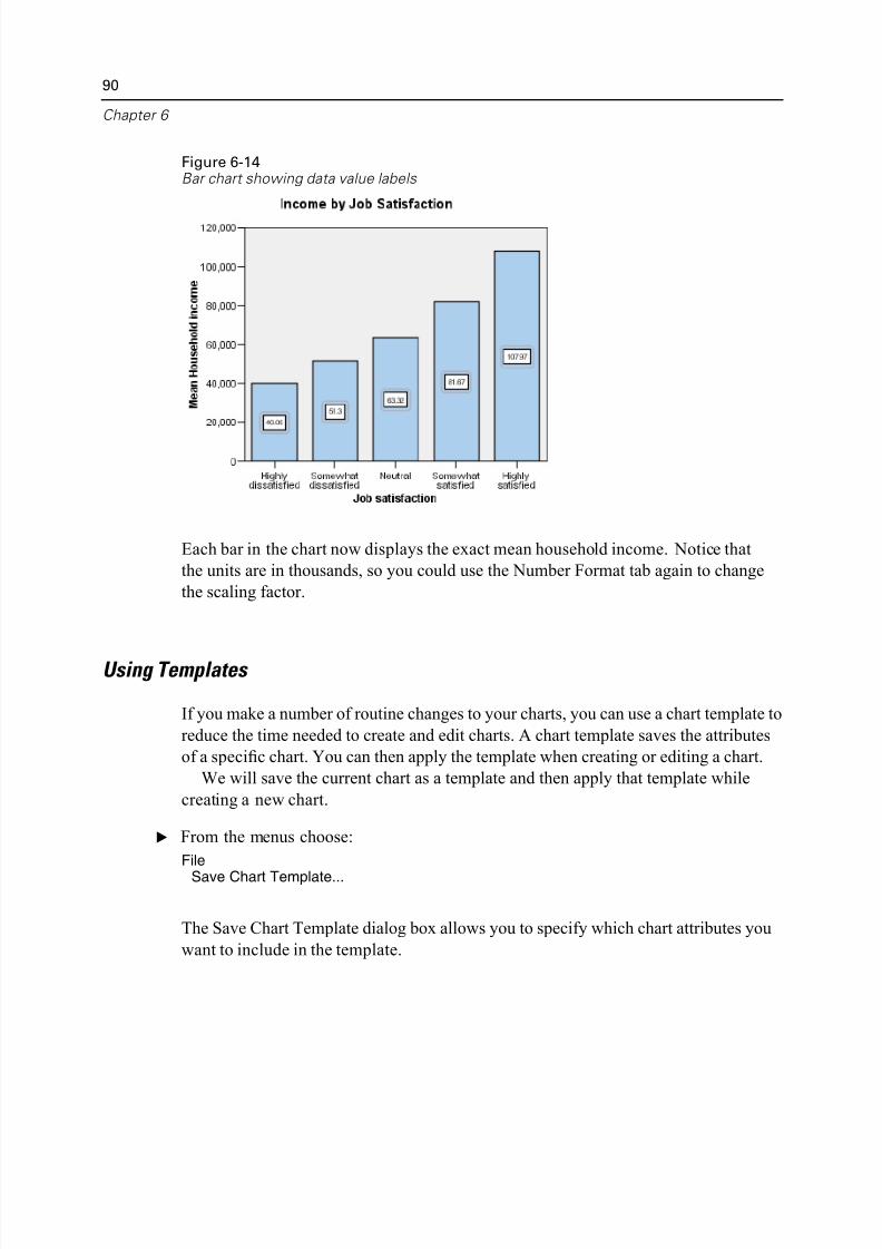
5/11/2018 SPSS Statistics Brief Guide 17.0 - slidepdf.com
http://slidepdf.com/reader/full/spss-statistics-brief-guide-170-55a2339b08a28 104/224
90
Chapter 6
Figure 6-14Bar chart showing data value labels
Each bar in the chart now displays the exact mean household income. Notice that
the units are in thousands, so you could use the Number Format tab again to chang
the scaling factor.
Using Templates
If you make a number of routine changes to your charts, you can use a chart templat
reduce the time needed to create and edit charts. A chart template saves the attribute
of a specific chart. You can then apply the template when creating or editing a chart
We will save the current chart as a template and then apply that template while
creating a new chart.
E From the menus choose:
File
Save Chart Template...
The Save Chart Template dialog box allows you to specify which chart attributes yo
want to include in the template.
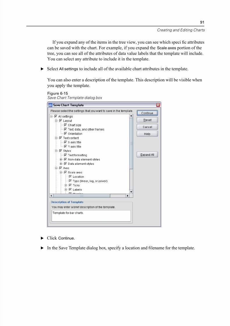
5/11/2018 SPSS Statistics Brief Guide 17.0 - slidepdf.com
http://slidepdf.com/reader/full/spss-statistics-brief-guide-170-55a2339b08a28 105/224
Creating and Editing Ch
If you expand any of the items in the tree view, you can see which specific attribu
can be saved with the chart. For example, if you expand the Scale axes portion of th
tree, you can see all of the attributes of data value labels that the template will inclu
You can select any attribute to include it in the template.
E Select All settings to include all of the available chart attributes in the template.
You can also enter a description of the template. This description will be visible wh
you apply the template.
Figure 6-15Save Chart Template dialog box
E Click Continue.
E In the Save Template dialog box, specify a location and filename for the template.
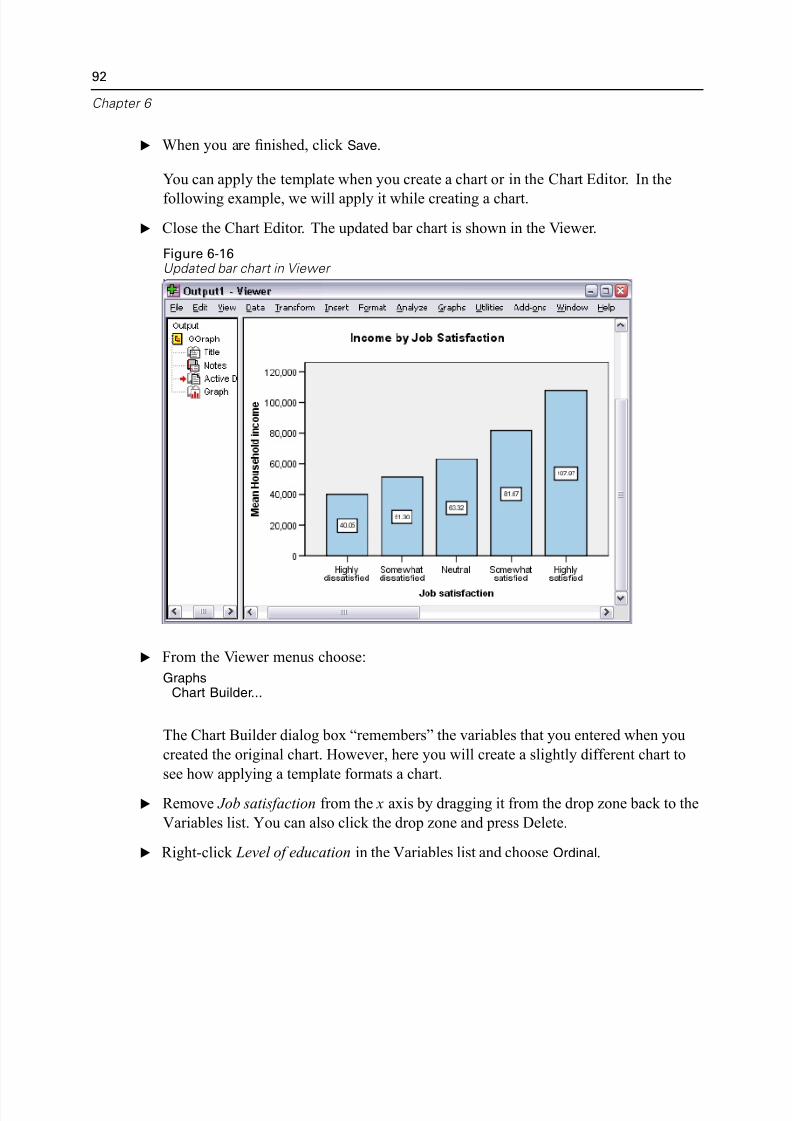
5/11/2018 SPSS Statistics Brief Guide 17.0 - slidepdf.com
http://slidepdf.com/reader/full/spss-statistics-brief-guide-170-55a2339b08a28 106/224
92
Chapter 6
E When you are finished, click Save.
You can apply the template when you create a chart or in the Chart Editor. In the
following example, we will apply it while creating a chart.
E Close the Chart Editor. The updated bar chart is shown in the Viewer.
Figure 6-16Updated bar chart in Viewer
E From the Viewer menus choose:
GraphsChart Builder...
The Chart Builder dialog box “remembers” the variables that you entered when you
created the original chart. However, here you will create a slightly different chart to
see how applying a template formats a chart.
E Remove Job satisfaction from the x axis by dragging it from the drop zone back to t
Variables list. You can also click the drop zone and press Delete.
E Right-click Level of education in the Variables list and choose Ordinal.
5/11/2018 SPSS Statistics Brief Guide 17.0 - slidepdf.com
http://slidepdf.com/reader/full/spss-statistics-brief-guide-170-55a2339b08a28 107/224
Creating and Editing Ch
E Drag Level of education from the Variables list to the x axis drop zone.
Because the title is now inaccurate, we are going to delete it.
E On the Titles/Footnotes tab, deselect Title 1.
Now we are going to specify the template to apply to the new chart.
E Click Options.
E In the Templates group in the Options dialog box, click Add.
E In the Find Template Files dialog box, locate the template file that you previously
saved using the Save Chart Template dialog box.
E Select that file and click Open.
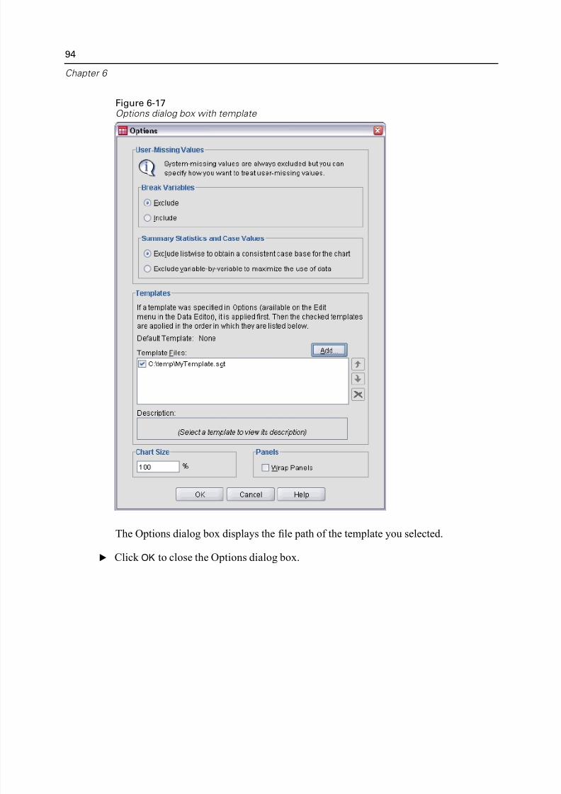
5/11/2018 SPSS Statistics Brief Guide 17.0 - slidepdf.com
http://slidepdf.com/reader/full/spss-statistics-brief-guide-170-55a2339b08a28 108/224
94
Chapter 6
Figure 6-17Options dialog box with template
The Options dialog box displays the file path of the template you selected.
E Click OK to close the Options dialog box.
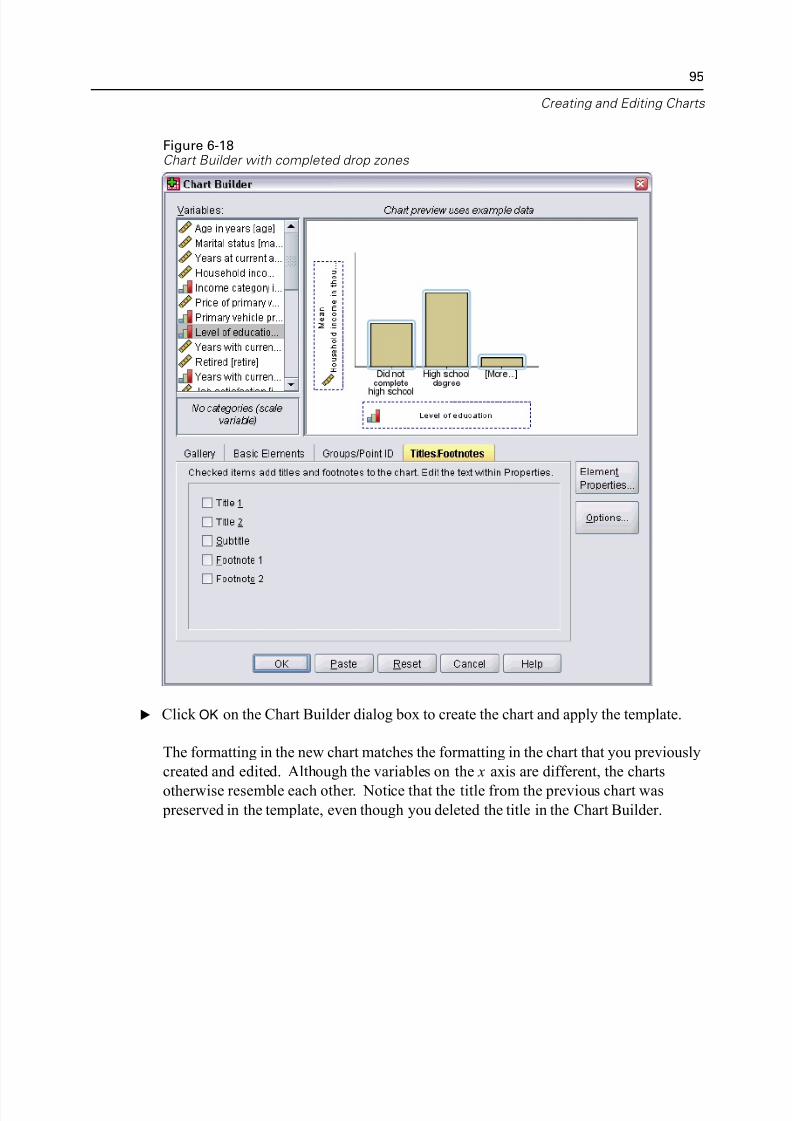
5/11/2018 SPSS Statistics Brief Guide 17.0 - slidepdf.com
http://slidepdf.com/reader/full/spss-statistics-brief-guide-170-55a2339b08a28 109/224
Creating and Editing Ch
Figure 6-18Chart Builder with completed drop zones
E Click OK on the Chart Builder dialog box to create the chart and apply the template.
The formatting in the new chart matches the formatting in the chart that you previou
created and edited. Although the variables on the x axis are different, the charts
other wise resemble each other. Notice that the title from the previous chart was
preserved in the template, even though you deleted the title in the Chart Builder.
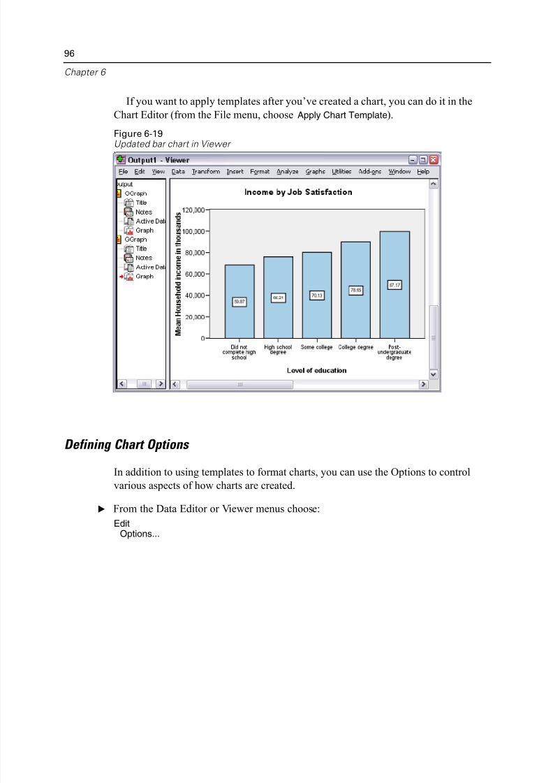
5/11/2018 SPSS Statistics Brief Guide 17.0 - slidepdf.com
http://slidepdf.com/reader/full/spss-statistics-brief-guide-170-55a2339b08a28 110/224
96
Chapter 6
If you want to apply templates after you’ve created a chart, you can do it in the
Chart Editor (from the File menu, choose Apply Chart Template).
Figure 6-19Updated bar chart in Viewer
Defining Chart Options
In addition to using templates to format charts, you can use the Options to control
various aspects of how charts are created.
E From the Data Editor or Viewer menus choose:
EditOptions...
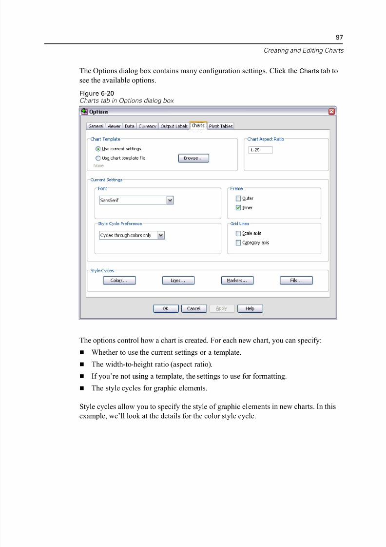
5/11/2018 SPSS Statistics Brief Guide 17.0 - slidepdf.com
http://slidepdf.com/reader/full/spss-statistics-brief-guide-170-55a2339b08a28 111/224
Creating and Editing Ch
The Options dialog box contains many configuration settings. Click the Charts tab
see the available options.
Figure 6-20Charts tab in Options dialog box
The options control how a chart is created. For each new chart, you can specify:
Whether to use the current settings or a template.
The width-to-height ratio (aspect ratio).
If you’re not using a template, the settings to use for formatting.
The style cycles for graphic elements.
Style cycles allow you to specify the style of graphic elements in new charts. In thi
example, we’ll look at the details for the color style cycle.
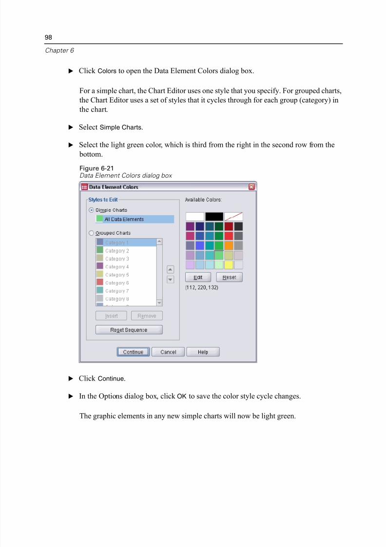
5/11/2018 SPSS Statistics Brief Guide 17.0 - slidepdf.com
http://slidepdf.com/reader/full/spss-statistics-brief-guide-170-55a2339b08a28 112/224
98
Chapter 6
E Click Colors to open the Data Element Colors dialog box.
For a simple chart, the Chart Editor uses one style that you specify. For grouped cha
the Chart Editor uses a set of styles that it cycles through for each group (category)
the chart.
E Select Simple Charts.
E Select the light green color, which is third from the right in the second row from th
bottom.
Figure 6-21Data Element Colors dialog box
E
Click Continue
.
E In the Options dialog box, click OK to save the color style cycle changes.
The graphic elements in any new simple charts will now be light green.
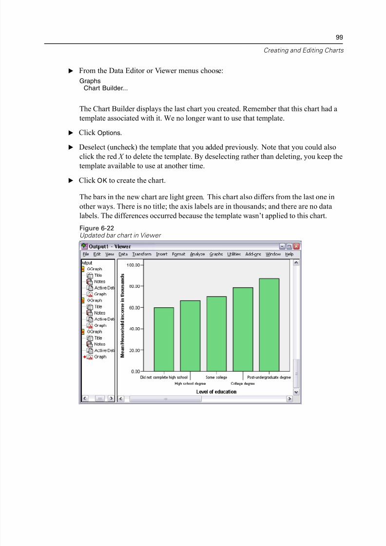
5/11/2018 SPSS Statistics Brief Guide 17.0 - slidepdf.com
http://slidepdf.com/reader/full/spss-statistics-brief-guide-170-55a2339b08a28 113/224
Creating and Editing Ch
E From the Data Editor or Viewer menus choose:
GraphsChart Builder...
The Chart Builder displays the last chart you created. Remember that this chart had
template associated with it. We no longer want to use that template.
E Click Options.
E Deselect (uncheck) the template that you added previously. Note that you could als
click the red X to delete the template. By deselecting rather than deleting, you keep
template available to use at another time.
E Click OK to create the chart.
The bars in the new chart are light green. This chart also differs from the last one in
other ways. There is no title; the axis labels are in thousands; and there are no data
labels. The differences occurred because the template wasn’t applied to this chart.
Figure 6-22Updated bar chart in Viewer
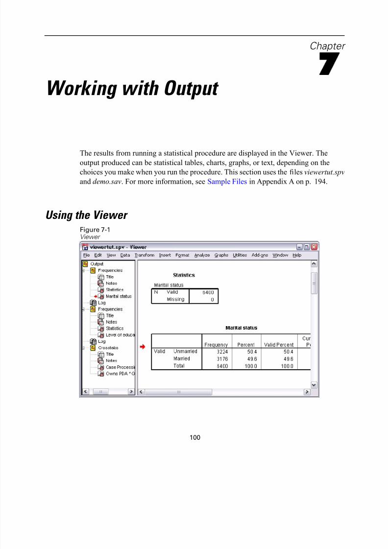
5/11/2018 SPSS Statistics Brief Guide 17.0 - slidepdf.com
http://slidepdf.com/reader/full/spss-statistics-brief-guide-170-55a2339b08a28 114/224
Chapt
7
Working with Output
The results from running a statistical procedure are displayed in the Viewer. The
output produced can be statistical tables, charts, graphs, or text, depending on the
choices you make when you run the procedure. This section uses the files viewertut.
and demo.sav. For more information, see Sample Files in Appendix A on p. 194.
Using the Viewer Figure 7-1Viewer
100
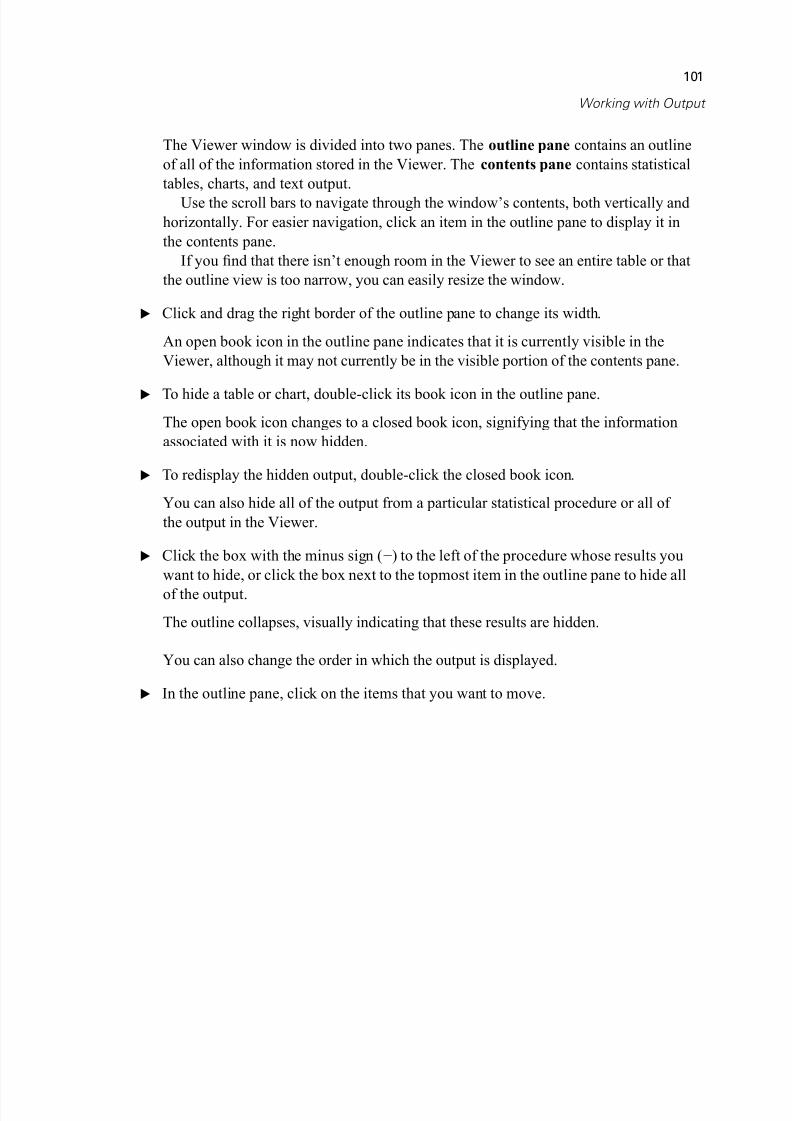
5/11/2018 SPSS Statistics Brief Guide 17.0 - slidepdf.com
http://slidepdf.com/reader/full/spss-statistics-brief-guide-170-55a2339b08a28 115/224
Working with Ou
The Viewer window is divided into two panes. The outline pane contains an outlin
of all of the information stored in the Viewer. The contents pane contains statistica
tables, charts, and text output.
Use the scroll bars to navigate through the window’s contents, both vertically an
horizontally. For easier navigation, click an item in the outline pane to display it in
the contents pane.
If you find that there isn’t enough room in the Viewer to see an entire table or tha
the outline view is too narrow, you can easily resize the window.
E Click and drag the right border of the outline pane to change its width.
An open book icon in the outline pane indicates that it is currently visible in the
Viewer, although it may not currently be in the visible portion of the contents pane.
E To hide a table or chart, double-click its book icon in the outline pane.
The open book icon changes to a closed book icon, signifying that the information
associated with it is now hidden.
E To redisplay the hidden output, double-click the closed book icon.
You can also hide all of the output from a particular statistical procedure or all of
the output in the Viewer.
E Click the box with the minus sign (−) to the left of the procedure whose results you
want to hide, or click the box next to the topmost item in the outline pane to hide al
of the output.
The outline collapses, visually indicating that these results are hidden.
You can also change the order in which the output is displayed.
E In the outline pane, click on the items that you want to move.
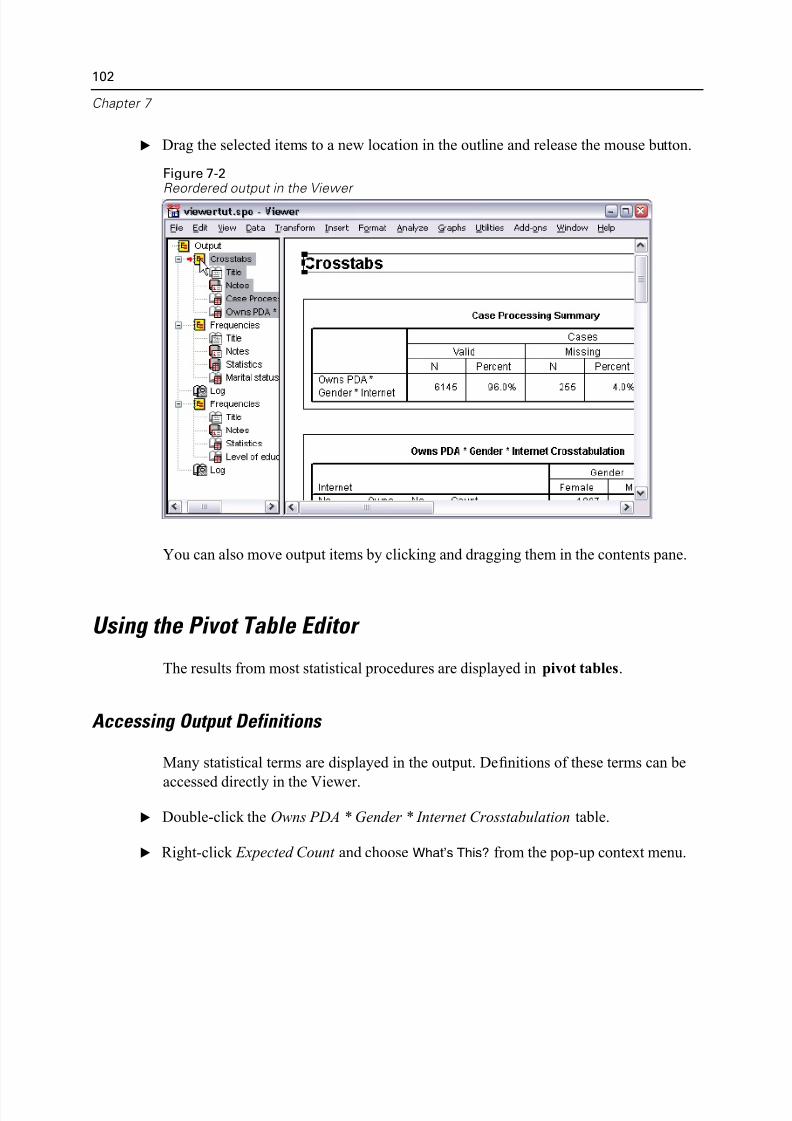
5/11/2018 SPSS Statistics Brief Guide 17.0 - slidepdf.com
http://slidepdf.com/reader/full/spss-statistics-brief-guide-170-55a2339b08a28 116/224
102
Chapter 7
E Drag the selected items to a new location in the outline and release the mouse button
Figure 7-2Reordered output in the Viewer
You can also move output items by clicking and dragging them in the contents pane
Using the Pivot Table Editor
The results from most statistical procedures are displayed in pivot tables.
Accessing Output Definitions
Many statistical terms are displayed in the output. Definitions of these terms can be
accessed directly in the Viewer.
E Double-click the Owns PDA * Gender * Internet Crosstabulation table.
E Right-click Expected Count and choose What’s This? from the pop-up context menu
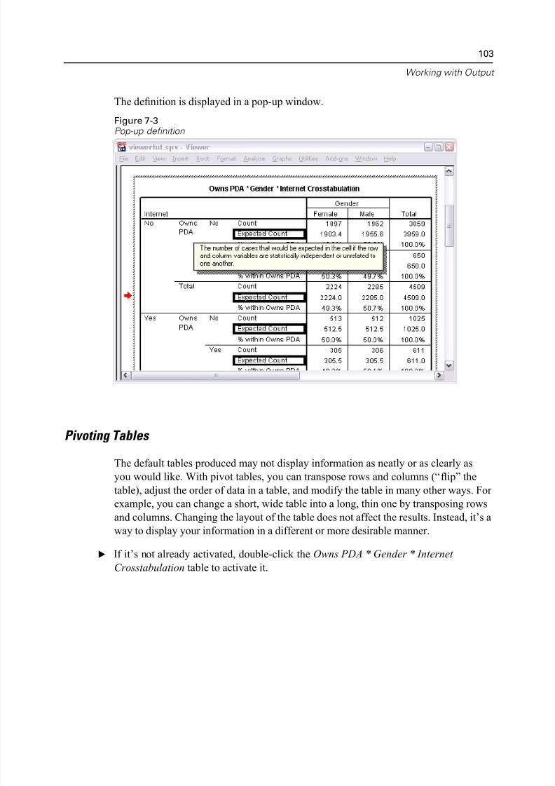
5/11/2018 SPSS Statistics Brief Guide 17.0 - slidepdf.com
http://slidepdf.com/reader/full/spss-statistics-brief-guide-170-55a2339b08a28 117/224
Working with Ou
The definition is displayed in a pop-up window.
Figure 7-3Pop-up definition
Pivoting Tables
The default tables produced may not display information as neatly or as clearly as
you would like. With pivot tables, you can transpose rows and columns (“flip” the
table), adjust the order of data in a table, and modify the table in many other ways. F
example, you can change a short, wide table into a long, thin one by transposing row
and columns. Changing the layout of the table does not affect the results. Instead, it
way to display your information in a different or more desirable manner.
E If it’s not already activated, double-click the Owns PDA * Gender * Internet
Crosstabulation table to activate it.
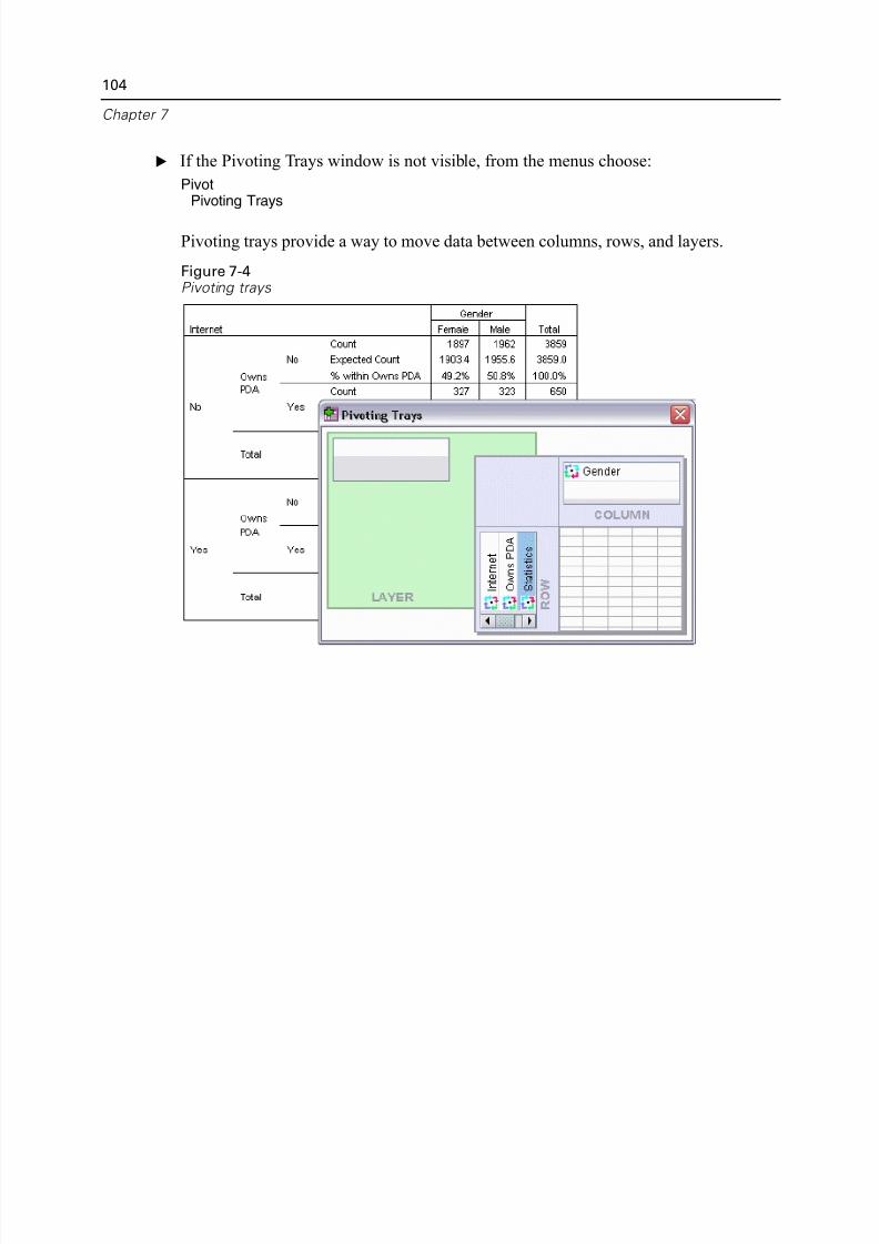
5/11/2018 SPSS Statistics Brief Guide 17.0 - slidepdf.com
http://slidepdf.com/reader/full/spss-statistics-brief-guide-170-55a2339b08a28 118/224
104
Chapter 7
E If the Pivoting Trays window is not visible, from the menus choose:
PivotPivoting Trays
Pivoting trays provide a way to move data between columns, rows, and layers.
Figure 7-4Pivoting trays
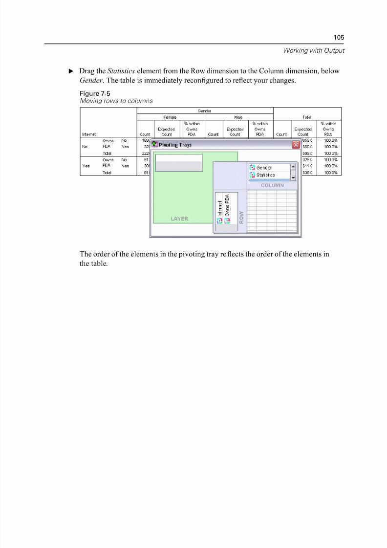
5/11/2018 SPSS Statistics Brief Guide 17.0 - slidepdf.com
http://slidepdf.com/reader/full/spss-statistics-brief-guide-170-55a2339b08a28 119/224
Working with Ou
E Drag the Statistics element from the Row dimension to the Column dimension, belo
Gender . The table is immediately reconfigured to reflect your changes.
Figure 7-5Moving rows to columns
The order of the elements in the pivoting tray reflects the order of the elements in
the table.
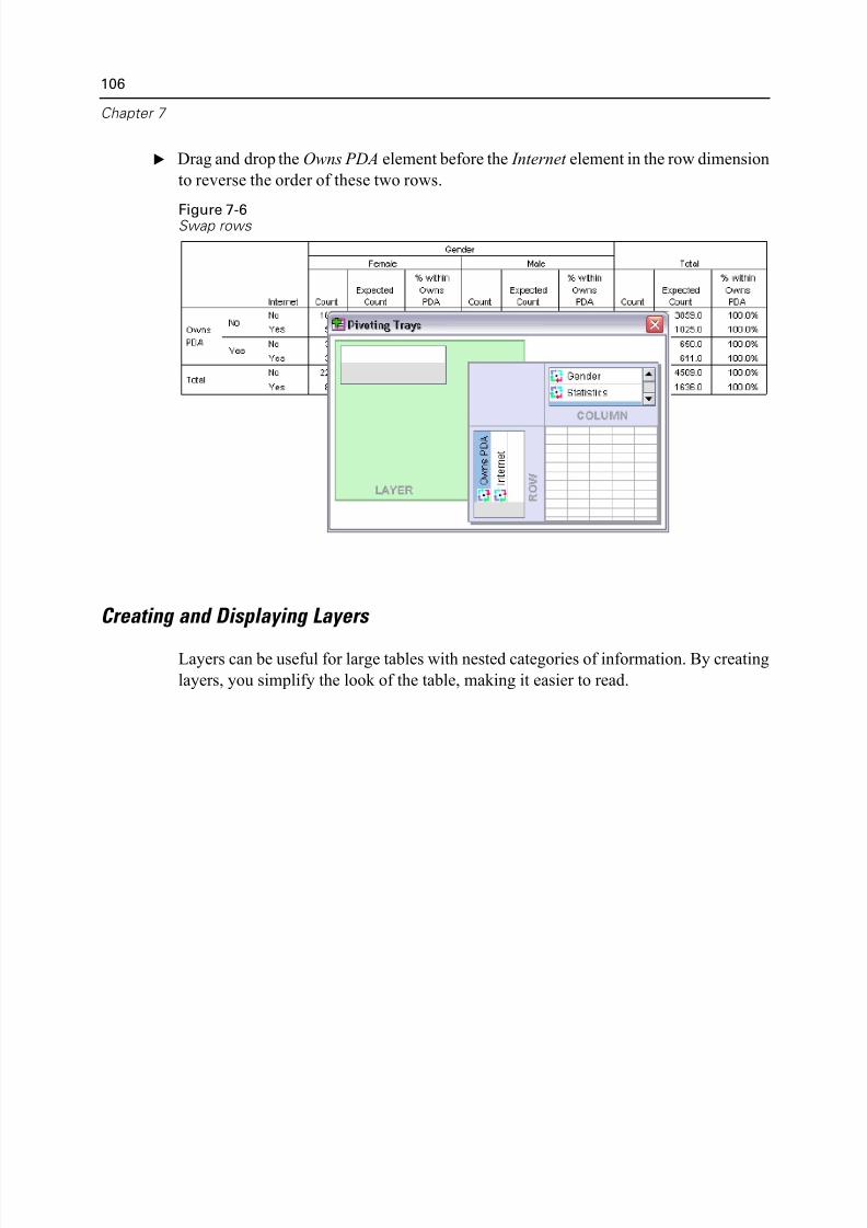
5/11/2018 SPSS Statistics Brief Guide 17.0 - slidepdf.com
http://slidepdf.com/reader/full/spss-statistics-brief-guide-170-55a2339b08a28 120/224
106
Chapter 7
E Drag and drop the Owns PDA element before the Internet element in the row dimens
to reverse the order of these two rows.
Figure 7-6Swap rows
Creating and Displaying Layers
Layers can be useful for large tables with nested categories of information. By creat
layers, you simplify the look of the table, making it easier to read.
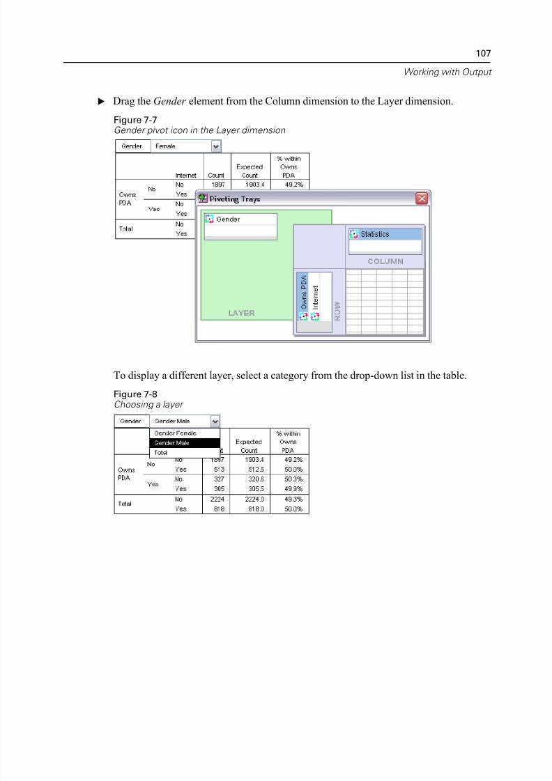
5/11/2018 SPSS Statistics Brief Guide 17.0 - slidepdf.com
http://slidepdf.com/reader/full/spss-statistics-brief-guide-170-55a2339b08a28 121/224
Working with Ou
E Drag the Gender element from the Column dimension to the Layer dimension.
Figure 7-7Gender pivot icon in the Layer dimension
To display a different layer, select a category from the drop-down list in the table.
Figure 7-8
Choosing a layer
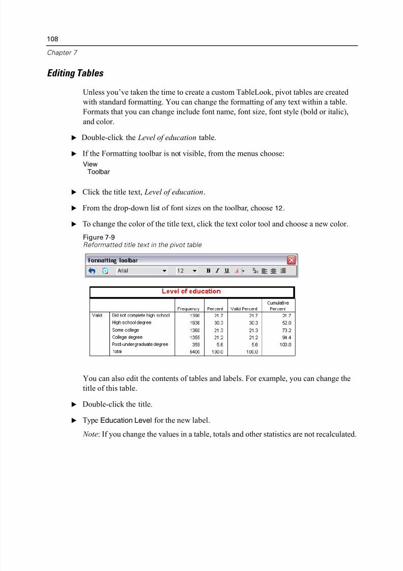
5/11/2018 SPSS Statistics Brief Guide 17.0 - slidepdf.com
http://slidepdf.com/reader/full/spss-statistics-brief-guide-170-55a2339b08a28 122/224
108
Chapter 7
Editing Tables
Unless you’ve taken the time to create a custom TableLook, pivot tables are created
with standard formatting. You can change the formatting of any text within a table.Formats that you can change include font name, font size, font style (bold or italic)
and color.
E Double-click the Level of education table.
E If the Formatting toolbar is not visible, from the menus choose:
ViewToolbar
E Click the title text, Level of education.
E From the drop-down list of font sizes on the toolbar, choose 12.
E To change the color of the title text, click the text color tool and choose a new color
Figure 7-9Reformatted title text in the pivot table
You can also edit the contents of tables and labels. For example, you can change th
title of this table.
E Double-click the title.
E Type Education Level for the new label.
Note: If you change the values in a table, totals and other statistics are not recalculat
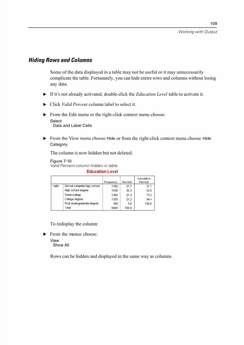
5/11/2018 SPSS Statistics Brief Guide 17.0 - slidepdf.com
http://slidepdf.com/reader/full/spss-statistics-brief-guide-170-55a2339b08a28 123/224
Working with Ou
Hiding Rows and Columns
Some of the data displayed in a table may not be useful or it may unnecessarily
complicate the table. Fortunately, you can hide entire rows and columns without los
any data.
E If it’s not already activated, double-click the Education Level table to activate it.
E Click Valid Percent column label to select it.
E From the Edit menu or the right-click context menu choose:
SelectData and Label Cells
E From the View menu choose Hide or from the right-click context menu choose Hide
Category.
The column is now hidden but not deleted.
Figure 7-10Valid Percent column hidden in table
To redisplay the column:
E From the menus choose:
ViewShow All
Rows can be hidden and displayed in the same way as columns.
5/11/2018 SPSS Statistics Brief Guide 17.0 - slidepdf.com
http://slidepdf.com/reader/full/spss-statistics-brief-guide-170-55a2339b08a28 124/224
110
Chapter 7
Changing Data Display Formats
You can easily change the display format of data in pivot tables.
E If it’s not already activated, double-click the Education Level table to activate it.
E Click on the Percent column label to select it.
E From the Edit menu or the right-click context menu choose:
SelectData Cells
E From the Format menu or the right-click context menu choose Cell Properties.
E
Click the Format Value tab.
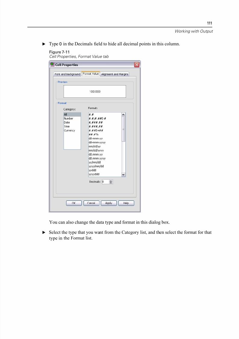
5/11/2018 SPSS Statistics Brief Guide 17.0 - slidepdf.com
http://slidepdf.com/reader/full/spss-statistics-brief-guide-170-55a2339b08a28 125/224
Working with Ou
E Type 0 in the Decimals field to hide all decimal points in this column.
Figure 7-11Cell Properties, Format Value tab
You can also change the data type and format in this dialog box.
E Select the type that you want from the Category list, and then select the format for th
type in the Format list.
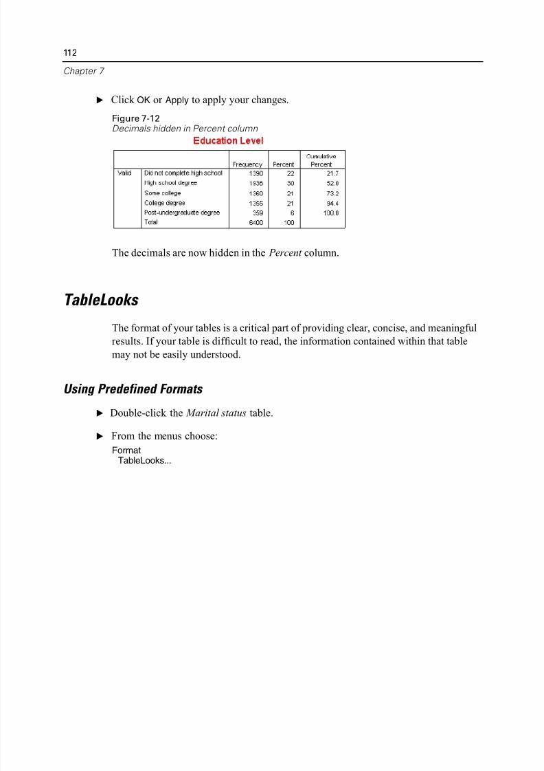
5/11/2018 SPSS Statistics Brief Guide 17.0 - slidepdf.com
http://slidepdf.com/reader/full/spss-statistics-brief-guide-170-55a2339b08a28 126/224
112
Chapter 7
E Click OK or Apply to apply your changes.
Figure 7-12Decimals hidden in Percent column
The decimals are now hidden in the Percent column.
TableLooks
The format of your tables is a critical part of providing clear, concise, and meaningf
results. If your table is dif ficult to read, the information contained within that table
may not be easily understood.
Using Predefined Formats
E Double-click the Marital status table.
E From the menus choose:
FormatTableLooks...
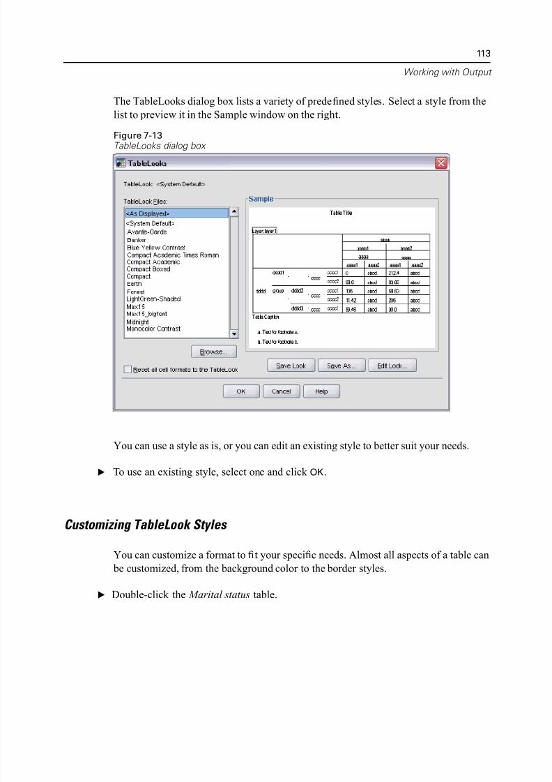
5/11/2018 SPSS Statistics Brief Guide 17.0 - slidepdf.com
http://slidepdf.com/reader/full/spss-statistics-brief-guide-170-55a2339b08a28 127/224
Working with Ou
The TableLooks dialog box lists a variety of predefined styles. Select a style from t
list to preview it in the Sample window on the right.
Figure 7-13TableLooks dialog box
You can use a style as is, or you can edit an existing style to better suit your needs.
E To use an existing style, select one and click OK.
Customizing TableLook Styles
You can customize a format to fit your specific needs. Almost all aspects of a table c
be customized, from the background color to the border styles.
E Double-click the Marital status table.
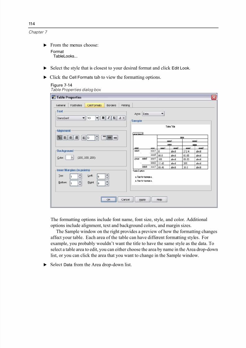
5/11/2018 SPSS Statistics Brief Guide 17.0 - slidepdf.com
http://slidepdf.com/reader/full/spss-statistics-brief-guide-170-55a2339b08a28 128/224
114
Chapter 7
E From the menus choose:
FormatTableLooks...
E Select the style that is closest to your desired format and click Edit Look.
E Click the Cell Formats tab to view the formatting options.
Figure 7-14Table Properties dialog box
The formatting options include font name, font size, style, and color. Additional
options include alignment, text and background colors, and margin sizes.
The Sample window on the right provides a preview of how the formatting chang
affect your table. Each area of the table can have different formatting styles. For
example, you probably wouldn’t want the title to have the same style as the data. Tselect a table area to edit, you can either choose the area by name in the Area drop-do
list, or you can click the area that you want to change in the Sample window.
E Select Data from the Area drop-down list.
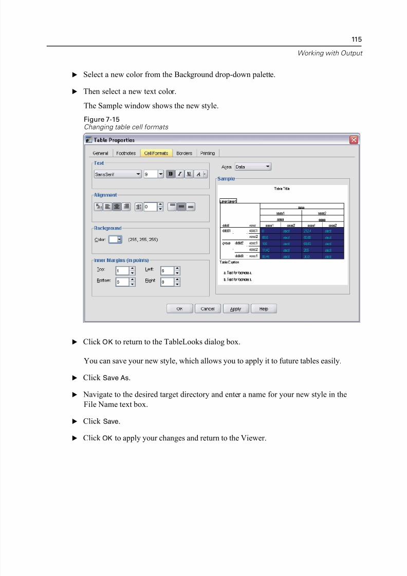
5/11/2018 SPSS Statistics Brief Guide 17.0 - slidepdf.com
http://slidepdf.com/reader/full/spss-statistics-brief-guide-170-55a2339b08a28 129/224
Working with Ou
E Select a new color from the Background drop-down palette.
E Then select a new text color.
The Sample window shows the new style.
Figure 7-15Changing table cell formats
E Click OK to return to the TableLooks dialog box.
You can save your new style, which allows you to apply it to future tables easily.
E Click Save As.
E Navigate to the desired target directory and enter a name for your new style in the
File Name text box.
E Click Save.
E Click OK to apply your changes and return to the Viewer.
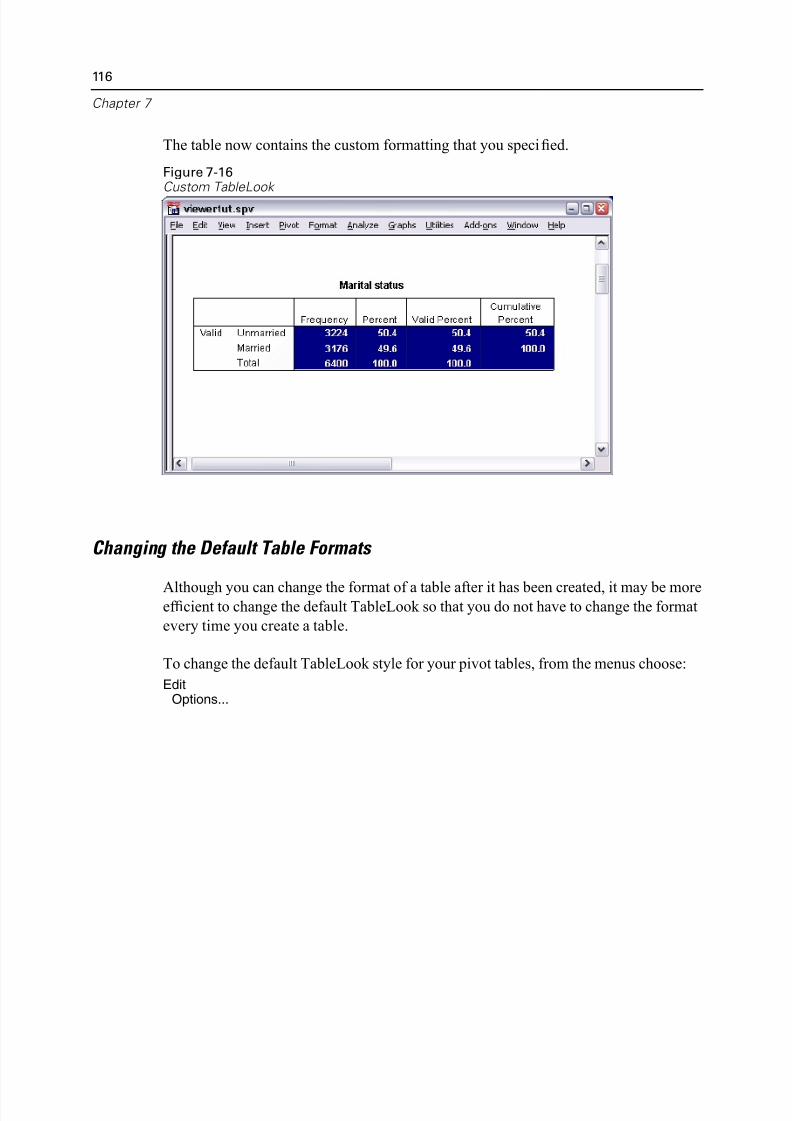
5/11/2018 SPSS Statistics Brief Guide 17.0 - slidepdf.com
http://slidepdf.com/reader/full/spss-statistics-brief-guide-170-55a2339b08a28 130/224
116
Chapter 7
The table now contains the custom formatting that you specified.
Figure 7-16Custom TableLook
Changing t he Default Table Formats
Although you can change the format of a table after it has been created, it may be mef ficient to change the default TableLook so that you do not have to change the form
every time you create a table.
To change the default TableLook style for your pivot tables, from the menus choose
EditOptions...
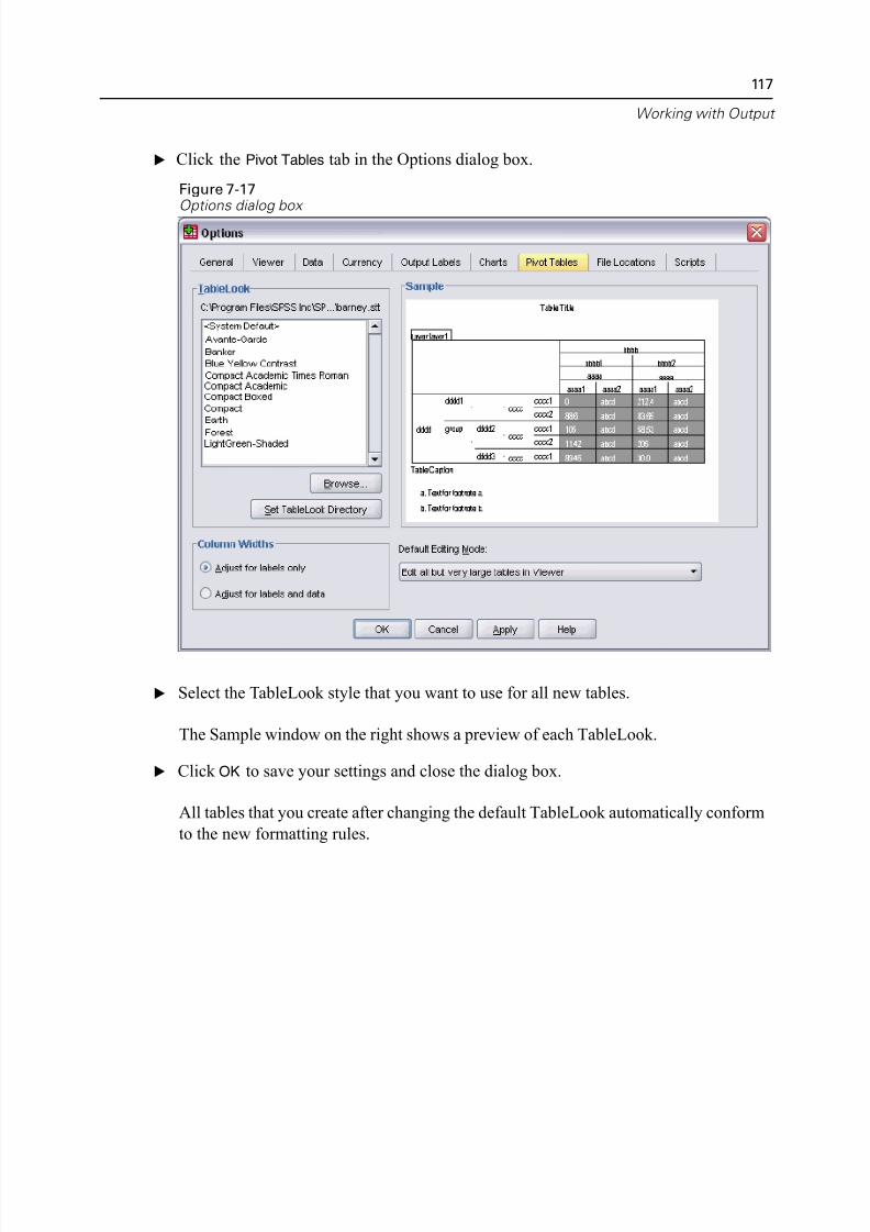
5/11/2018 SPSS Statistics Brief Guide 17.0 - slidepdf.com
http://slidepdf.com/reader/full/spss-statistics-brief-guide-170-55a2339b08a28 131/224
Working with Ou
E Click the Pivot Tables tab in the Options dialog box.
Figure 7-17Options dialog box
E Select the TableLook style that you want to use for all new tables.
The Sample window on the right shows a preview of each TableLook.
E Click OK to save your settings and close the dialog box.
All tables that you create after changing the default TableLook automatically confor
to the new formatting rules.
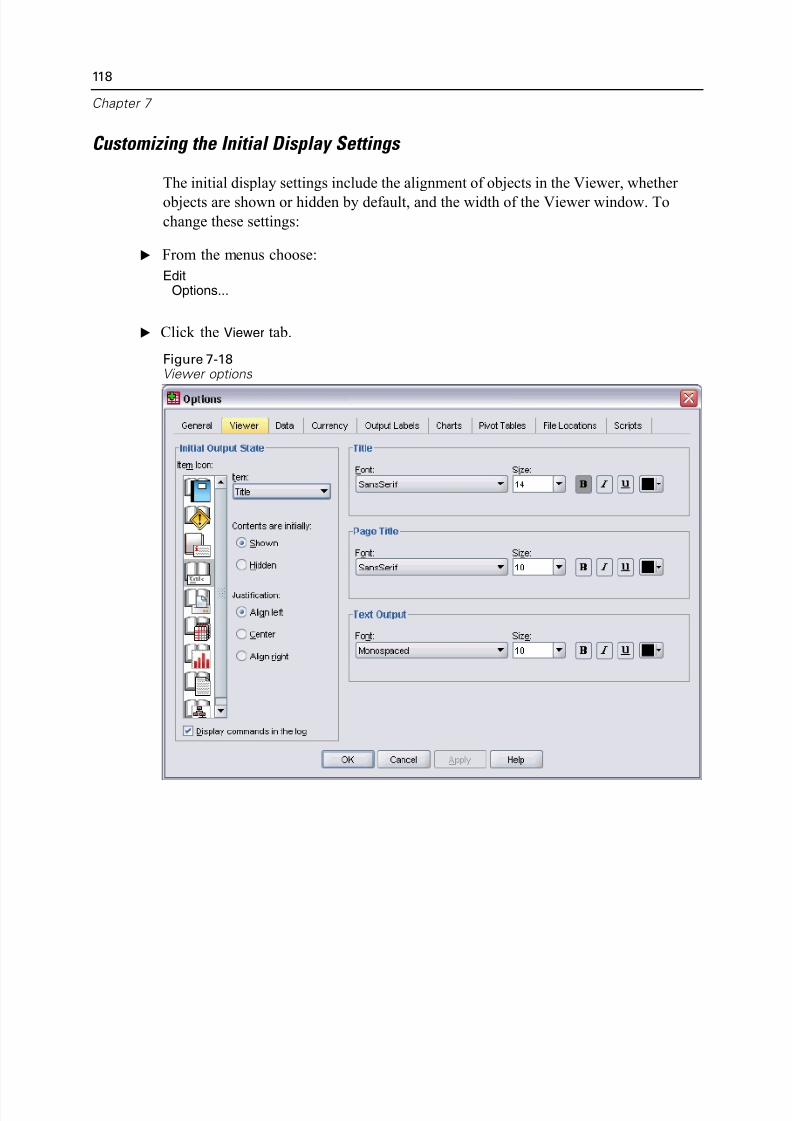
5/11/2018 SPSS Statistics Brief Guide 17.0 - slidepdf.com
http://slidepdf.com/reader/full/spss-statistics-brief-guide-170-55a2339b08a28 132/224
118
Chapter 7
Customizing the Initial Display Settings
The initial display settings include the alignment of objects in the Viewer, whether
objects are shown or hidden by default, and the width of the Viewer window. To
change these settings:
E From the menus choose:
EditOptions...
E Click the Viewer tab.
Figure 7-18Viewer options
5/11/2018 SPSS Statistics Brief Guide 17.0 - slidepdf.com
http://slidepdf.com/reader/full/spss-statistics-brief-guide-170-55a2339b08a28 133/224
Working with Ou
The settings are applied on an object-by-object basis. For example, you can custom
the way charts are displayed without making any changes to the way tables are
displayed. Simply select the object that you want to customize, and make the desire
changes.
E Click the Title icon to display its settings.
E Click Center to display all titles in the (horizontal) center of the Viewer.
You can also hide elements, such as the log and warning messages, that tend to clutt
your output. Double-clicking on an icon automatically changes that object’s display
property.
E Double-click the Warnings icon to hide warning messages in the output.
E Click OK to save your changes and close the dialog box.
Displaying Variable and Value Labels
In most cases, displaying the labels for variables and values is more effective than
displaying the variable name or the actual data value. There may be cases, however
when you want to display both the names and the labels.
E From the menus choose:
EditOptions...
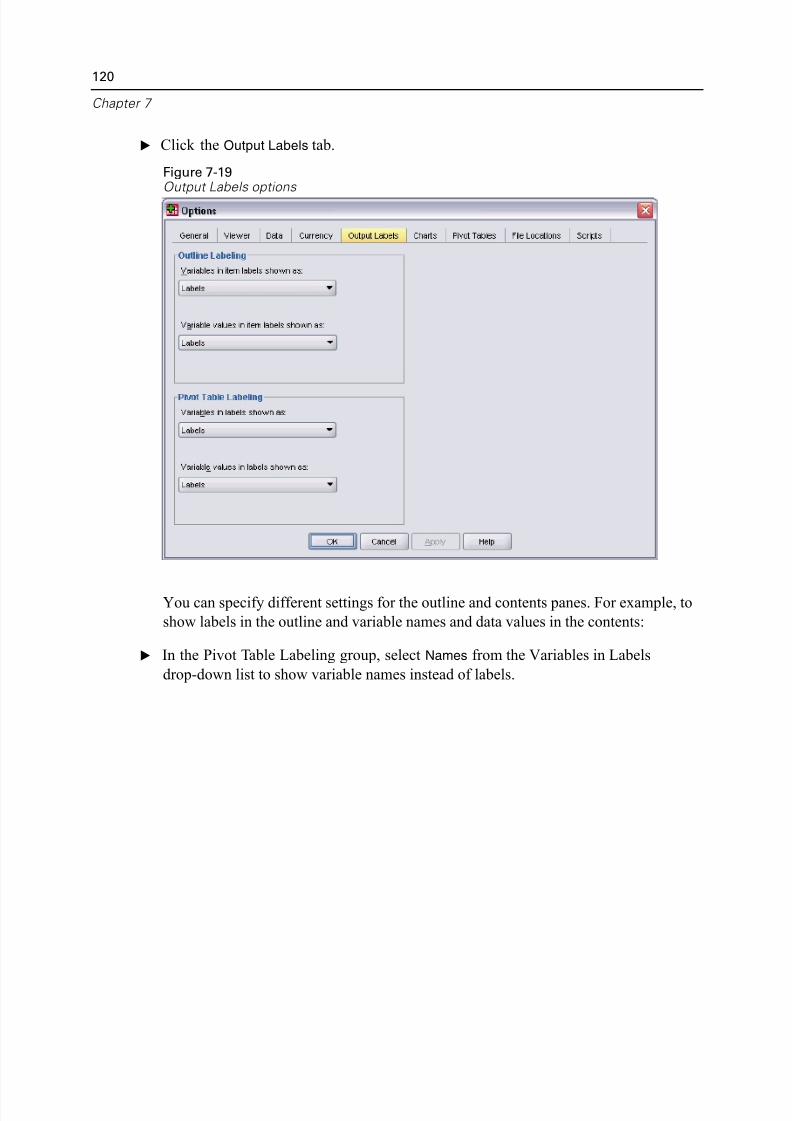
5/11/2018 SPSS Statistics Brief Guide 17.0 - slidepdf.com
http://slidepdf.com/reader/full/spss-statistics-brief-guide-170-55a2339b08a28 134/224
120
Chapter 7
E Click the Output Labels tab.
Figure 7-19Output Labels options
You can specify different settings for the outline and contents panes. For example,
show labels in the outline and variable names and data values in the contents:
E In the Pivot Table Labeling group, select Names from the Variables in Labels
drop-down list to show variable names instead of labels.
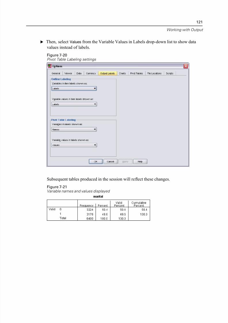
5/11/2018 SPSS Statistics Brief Guide 17.0 - slidepdf.com
http://slidepdf.com/reader/full/spss-statistics-brief-guide-170-55a2339b08a28 135/224
Working with Ou
E Then, select Values from the Variable Values in Labels drop-down list to show data
values instead of labels.
Figure 7-20Pivot Table Labeling settings
Subsequent tables produced in the session will reflect these changes.
Figure 7-21Variable names and values displayed
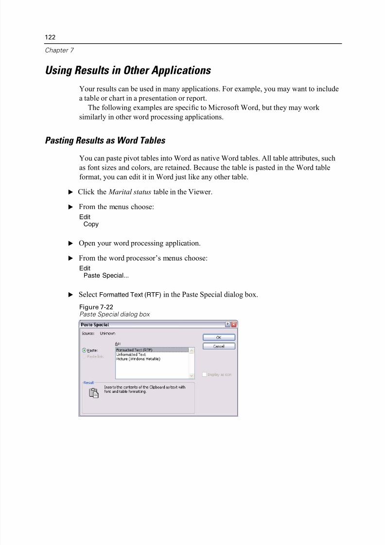
5/11/2018 SPSS Statistics Brief Guide 17.0 - slidepdf.com
http://slidepdf.com/reader/full/spss-statistics-brief-guide-170-55a2339b08a28 136/224
122
Chapter 7
Using Results in Other Applications
Your results can be used in many applications. For example, you may want to inclu
a table or chart in a presentation or report.
The following examples are specific to Microsoft Word, but they may work
similarly in other word processing applications.
Pasting Results as Word Tables
You can paste pivot tables into Word as native Word tables. All table attributes, suc
as font sizes and colors, are retained. Because the table is pasted in the Word table
format, you can edit it in Word just like any other table.
E Click the Marital status table in the Viewer.
E From the menus choose:
EditCopy
E Open your word processing application.
E From the word processor’s menus choose:
EditPaste Special...
E Select Formatted Text (RTF) in the Paste Special dialog box.
Figure 7-22Paste Special dialog box
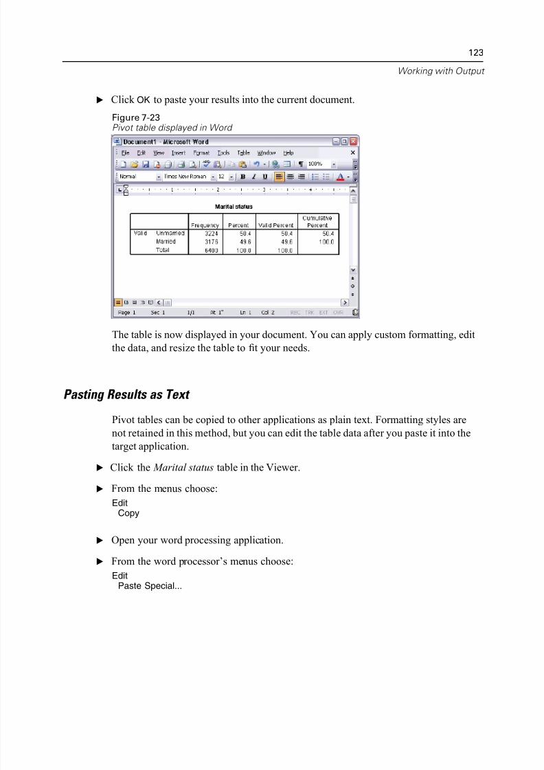
5/11/2018 SPSS Statistics Brief Guide 17.0 - slidepdf.com
http://slidepdf.com/reader/full/spss-statistics-brief-guide-170-55a2339b08a28 137/224
Working with Ou
E Click OK to paste your results into the current document.
Figure 7-23Pivot table displayed in Word
The table is now displayed in your document. You can apply custom formatting, ed
the data, and resize the table to fit your needs.
Pasting Results as Text
Pivot tables can be copied to other applications as plain text. Formatting styles are
not retained in this method, but you can edit the table data after you paste it into the
target application.
E Click the Marital status table in the Viewer.
E From the menus choose:
EditCopy
E Open your word processing application.
E From the word processor’s menus choose:
EditPaste Special...
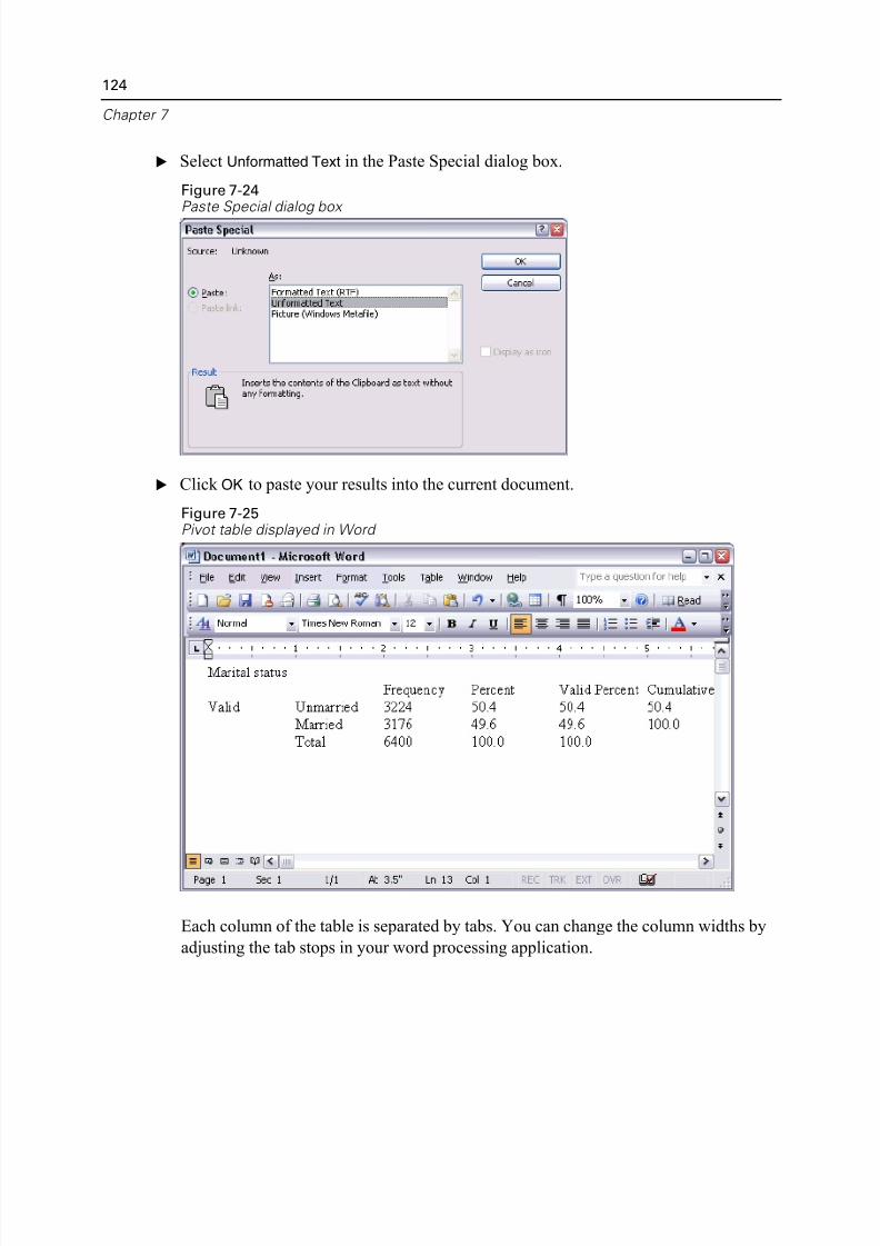
5/11/2018 SPSS Statistics Brief Guide 17.0 - slidepdf.com
http://slidepdf.com/reader/full/spss-statistics-brief-guide-170-55a2339b08a28 138/224
124
Chapter 7
E Select Unformatted Text in the Paste Special dialog box.
Figure 7-24Paste Special dialog box
E Click OK to paste your results into the current document.
Figure 7-25Pivot table displayed in Word
Each column of the table is separated by tabs. You can change the column widths b
adjusting the tab stops in your word processing application.
5/11/2018 SPSS Statistics Brief Guide 17.0 - slidepdf.com
http://slidepdf.com/reader/full/spss-statistics-brief-guide-170-55a2339b08a28 139/224
Working with Ou
Exporting Results to Microsoft Word, PowerPoint, and Excel Files
You can export results to a Microsoft Word , PowerPoint, or Excel file. You can exp
selected items or all items in the Viewer. This section uses the files msouttut.spv an
demo.sav. For more information, see Sample Files in Appendix A on p. 194.
Note: Export to PowerPoint is available only on Windows operating systems and is
not available with the Student Version.
In the Viewer’s outline pane, you can select specific items that you want to expo
You do not have to select specific items.
E From the Viewer menus choose:
FileExport...
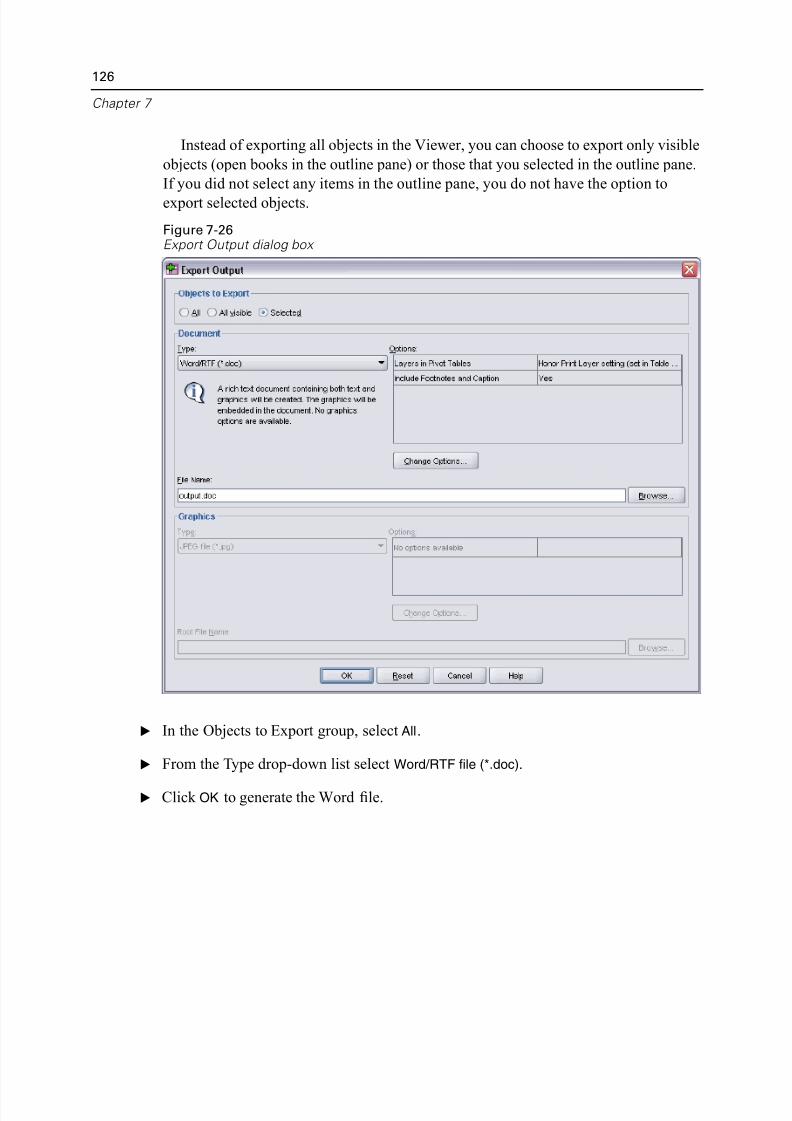
5/11/2018 SPSS Statistics Brief Guide 17.0 - slidepdf.com
http://slidepdf.com/reader/full/spss-statistics-brief-guide-170-55a2339b08a28 140/224
126
Chapter 7
Instead of exporting all objects in the Viewer, you can choose to export only visi
objects (open books in the outline pane) or those that you selected in the outline pan
If you did not select any items in the outline pane, you do not have the option to
export selected objects.
Figure 7-26Export Output dialog box
E In the Objects to Export group, select All.
E From the Type drop-down list select Word/RTF file (*.doc).
E Click OK to generate the Word file.
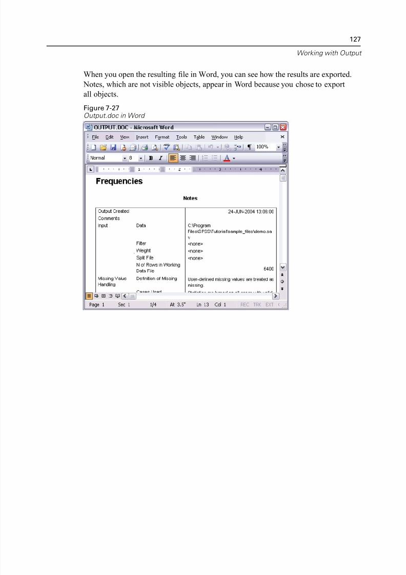
5/11/2018 SPSS Statistics Brief Guide 17.0 - slidepdf.com
http://slidepdf.com/reader/full/spss-statistics-brief-guide-170-55a2339b08a28 141/224
Working with Ou
When you open the resulting file in Word, you can see how the results are exported
Notes, which are not visible objects, appear in Word because you chose to export
all objects.
Figure 7-27Output.doc in Word
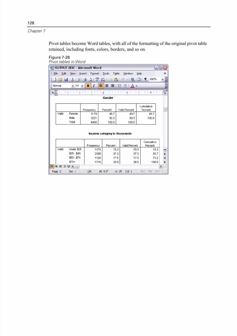
5/11/2018 SPSS Statistics Brief Guide 17.0 - slidepdf.com
http://slidepdf.com/reader/full/spss-statistics-brief-guide-170-55a2339b08a28 142/224
128
Chapter 7
Pivot tables become Word tables, with all of the formatting of the original pivot tab
retained, including fonts, colors, borders, and so on.
Figure 7-28Pivot tables in Word
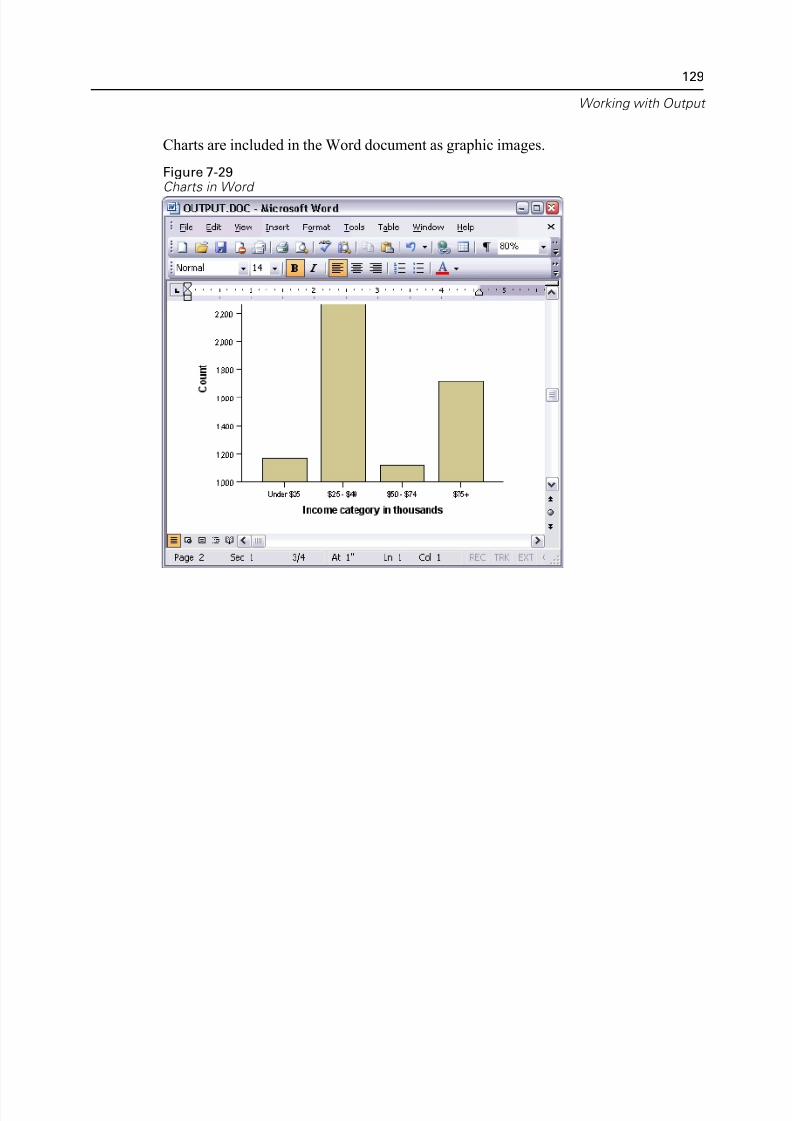
5/11/2018 SPSS Statistics Brief Guide 17.0 - slidepdf.com
http://slidepdf.com/reader/full/spss-statistics-brief-guide-170-55a2339b08a28 143/224
Working with Ou
Charts are included in the Word document as graphic images.
Figure 7-29Charts in Word
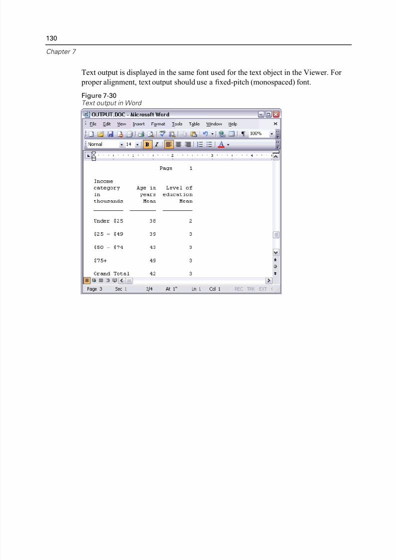
5/11/2018 SPSS Statistics Brief Guide 17.0 - slidepdf.com
http://slidepdf.com/reader/full/spss-statistics-brief-guide-170-55a2339b08a28 144/224
130
Chapter 7
Text output is displayed in the same font used for the text object in the Viewer. For
proper alignment, text output should use a fixed-pitch (monospaced) font.
Figure 7-30Text output in Word
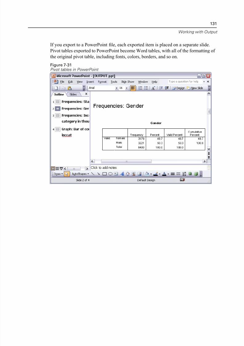
5/11/2018 SPSS Statistics Brief Guide 17.0 - slidepdf.com
http://slidepdf.com/reader/full/spss-statistics-brief-guide-170-55a2339b08a28 145/224
Working with Ou
If you export to a PowerPoint file, each exported item is placed on a separate slide.
Pivot tables exported to PowerPoint become Word tables, with all of the formatting
the original pivot table, including fonts, colors, borders, and so on.
Figure 7-31Pivot tables in PowerPoint
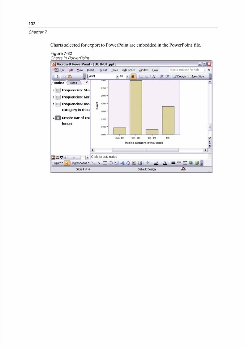
5/11/2018 SPSS Statistics Brief Guide 17.0 - slidepdf.com
http://slidepdf.com/reader/full/spss-statistics-brief-guide-170-55a2339b08a28 146/224
132
Chapter 7
Charts selected for export to PowerPoint are embedded in the PowerPoint file.
Figure 7-32Charts in PowerPoint
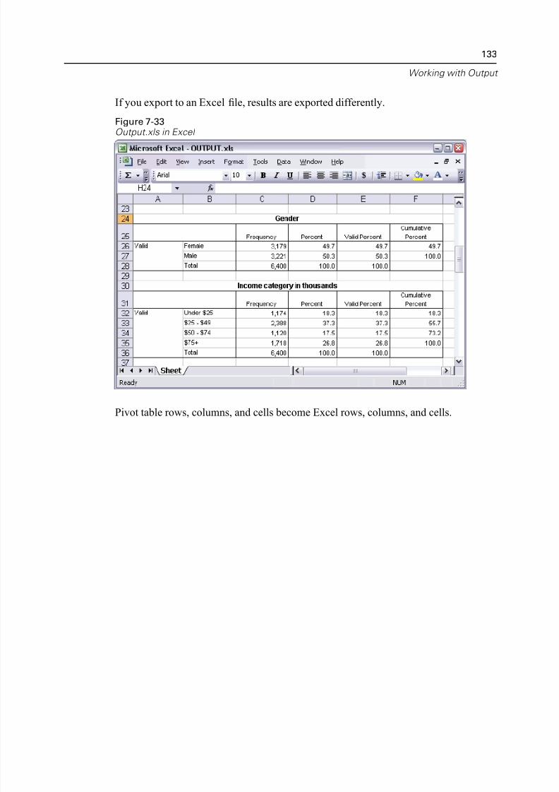
5/11/2018 SPSS Statistics Brief Guide 17.0 - slidepdf.com
http://slidepdf.com/reader/full/spss-statistics-brief-guide-170-55a2339b08a28 147/224
Working with Ou
If you export to an Excel file, results are exported differently.
Figure 7-33Output.xls in Excel
Pivot table rows, columns, and cells become Excel rows, columns, and cells.
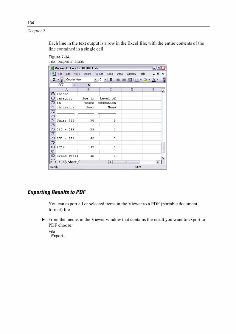
5/11/2018 SPSS Statistics Brief Guide 17.0 - slidepdf.com
http://slidepdf.com/reader/full/spss-statistics-brief-guide-170-55a2339b08a28 148/224
134
Chapter 7
Each line in the text output is a row in the Excel file, with the entire contents of the
line contained in a single cell.
Figure 7-34Text output in Excel
Exporting Results to PDF
You can export all or selected items in the Viewer to a PDF (portable document
format) file.
E From the menus in the Viewer window that contains the result you want to export to
PDF choose:
FileExport...
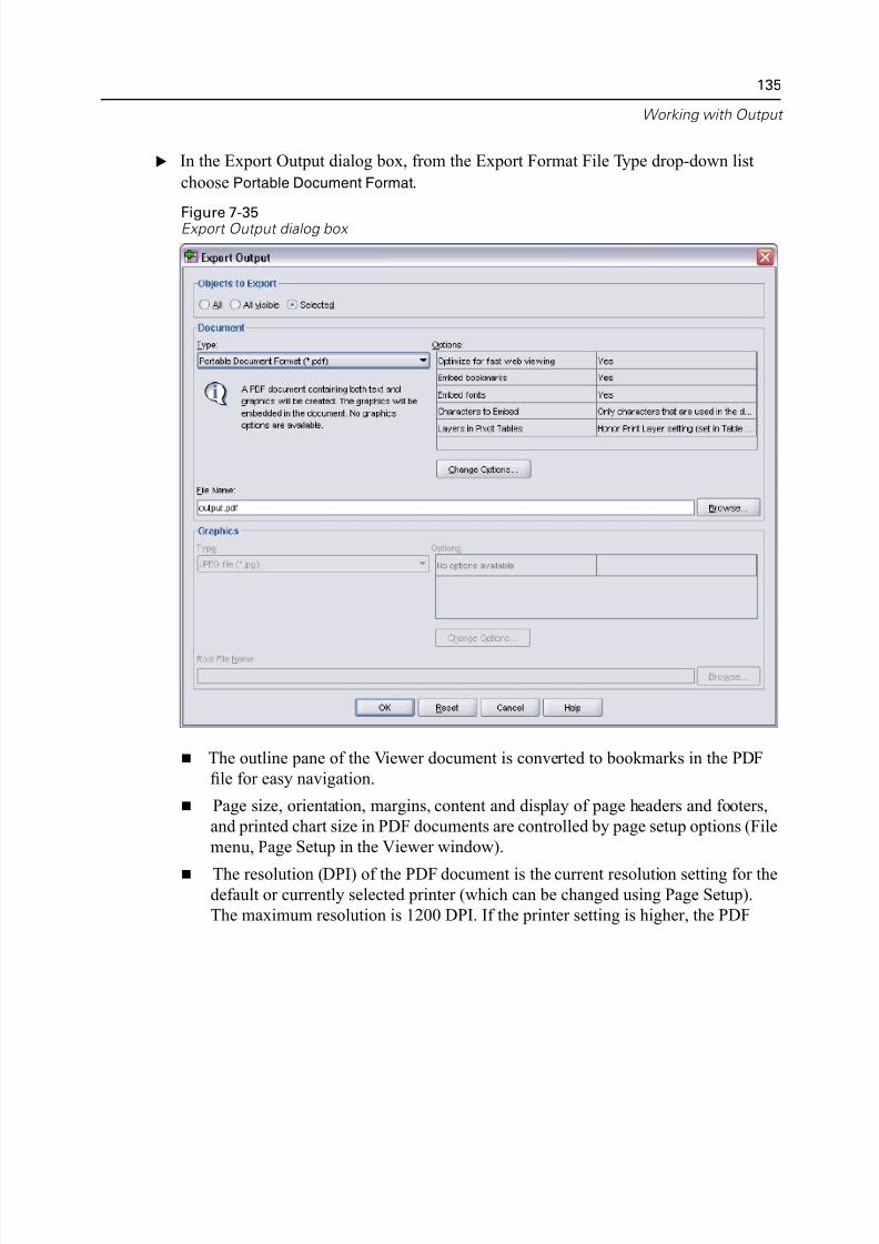
5/11/2018 SPSS Statistics Brief Guide 17.0 - slidepdf.com
http://slidepdf.com/reader/full/spss-statistics-brief-guide-170-55a2339b08a28 149/224
Working with Ou
E In the Export Output dialog box, from the Export Format File Type drop-down list
choose Portable Document Format.
Figure 7-35Export Output dialog box
The outline pane of the Viewer document is converted to bookmarks in the PDF
file for easy navigation.
Page size, orientation, margins, content and display of page headers and footer
and printed chart size in PDF documents are controlled by page setup options (F
menu, Page Setup in the Viewer window).
The resolution (DPI) of the PDF document is the current resolution setting for tdefault or currently selected printer (which can be changed using Page Setup).
The maximum resolution is 1200 DPI. If the printer setting is higher, the PDF
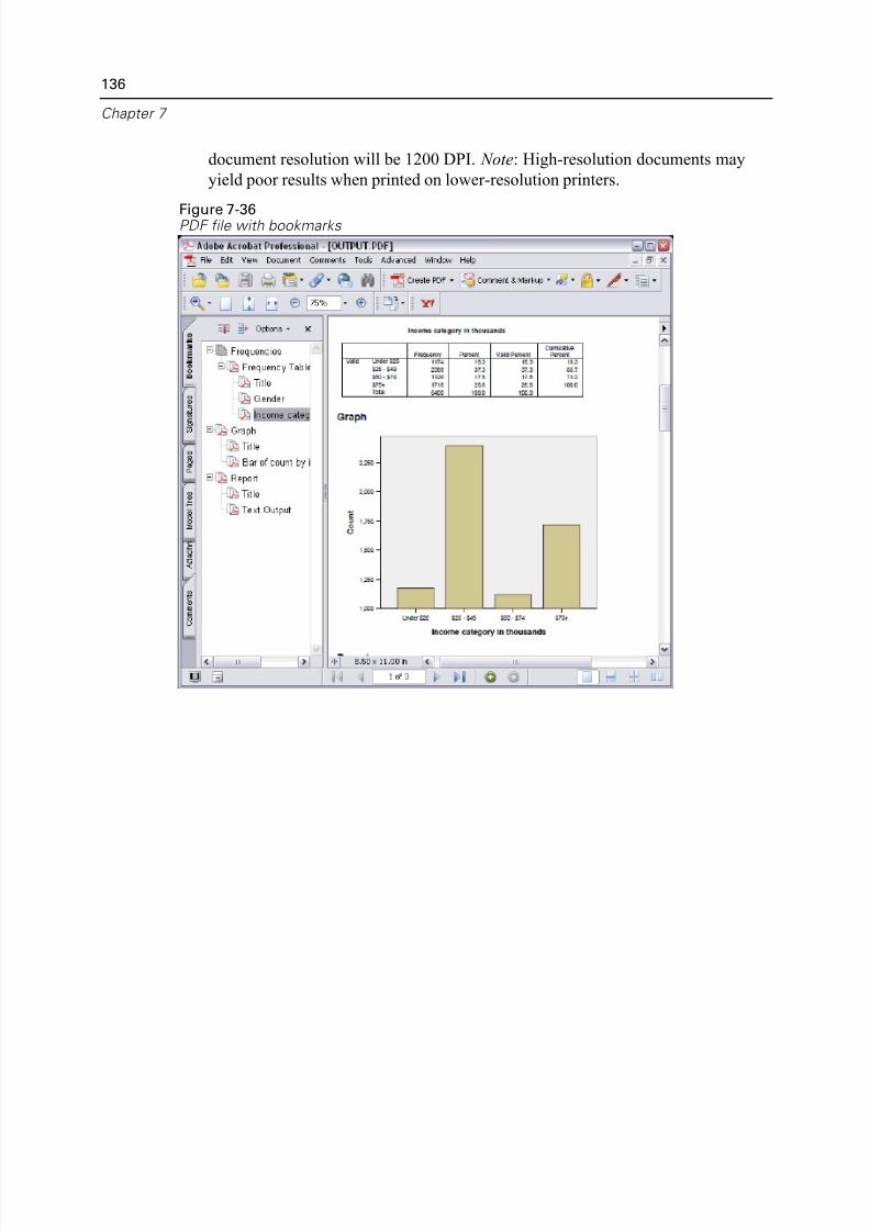
5/11/2018 SPSS Statistics Brief Guide 17.0 - slidepdf.com
http://slidepdf.com/reader/full/spss-statistics-brief-guide-170-55a2339b08a28 150/224
136
Chapter 7
document resolution will be 1200 DPI. Note: High-resolution documents may
yield poor results when printed on lower-resolution printers.
Figure 7-36PDF file with bookmarks
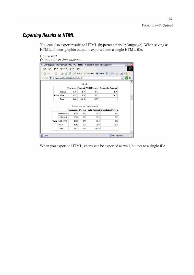
5/11/2018 SPSS Statistics Brief Guide 17.0 - slidepdf.com
http://slidepdf.com/reader/full/spss-statistics-brief-guide-170-55a2339b08a28 151/224
Working with Ou
Exporting Results to HTML
You can also export results to HTML (hypertext markup language). When saving a
HTML, all non-graphic output is exported into a single HTML file.
Figure 7-37Output.htm in Web browser
When you export to HTML, charts can be exported as well, but not to a single file.
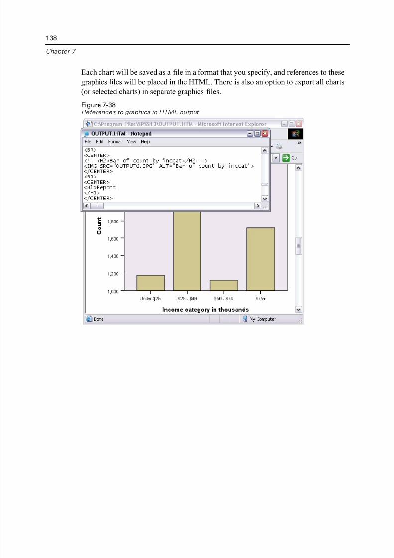
5/11/2018 SPSS Statistics Brief Guide 17.0 - slidepdf.com
http://slidepdf.com/reader/full/spss-statistics-brief-guide-170-55a2339b08a28 152/224
138
Chapter 7
Each chart will be saved as a file in a format that you specify, and references to the
graphics files will be placed in the HTML. There is also an option to export all char
(or selected charts) in separate graphics files.
Figure 7-38References to graphics in HTML output
5/11/2018 SPSS Statistics Brief Guide 17.0 - slidepdf.com
http://slidepdf.com/reader/full/spss-statistics-brief-guide-170-55a2339b08a28 153/224
Chapt
8
Working with Syntax
You can save and automate many common tasks by using the powerful command
language. It also provides some functionality not found in the menus and dialog
boxes. Most commands are accessible from the menus and dialog boxes. However
some commands and options are available only by using the command language.
The command language also allows you to save your jobs in a syntax file so that yocan repeat your analysis at a later date.
A command syntax file is simply a text file that contains SPSS Statistics syntax
commands. You can open a syntax window and type commands directly, but it is of
easier to let the dialog boxes do some or all of the work for you.
The examples in this chapter use the data file demo.sav. For more information, s
Sample Files in Appendix A on p. 194.
Note: Command syntax is not available with the Student Version.
Pasting Syntax The easiest way to create syntax is to use the Paste button located on most dialog box
E Open the data file demo.sav. For more information, see Sample Files in Appendix
A on p. 194.
E From the menus choose:
AnalyzeDescriptive Statistics
Frequencies...
139
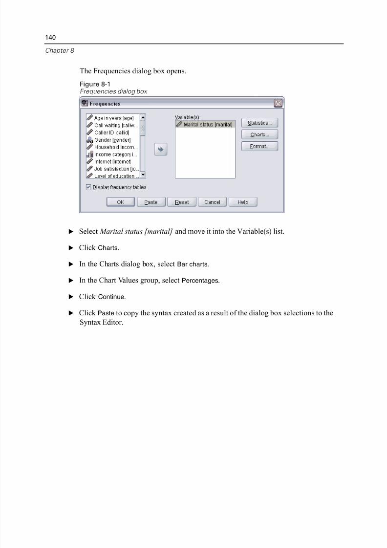
5/11/2018 SPSS Statistics Brief Guide 17.0 - slidepdf.com
http://slidepdf.com/reader/full/spss-statistics-brief-guide-170-55a2339b08a28 154/224
140
Chapter 8
The Frequencies dialog box opens.
Figure 8-1Frequencies dialog box
E Select Marital status [marital] and move it into the Variable(s) list.
E Click Charts.
E In the Charts dialog box, select Bar charts.
E In the Chart Values group, select Percentages.
E Click Continue.
E Click Paste to copy the syntax created as a result of the dialog box selections to the
Syntax Editor.
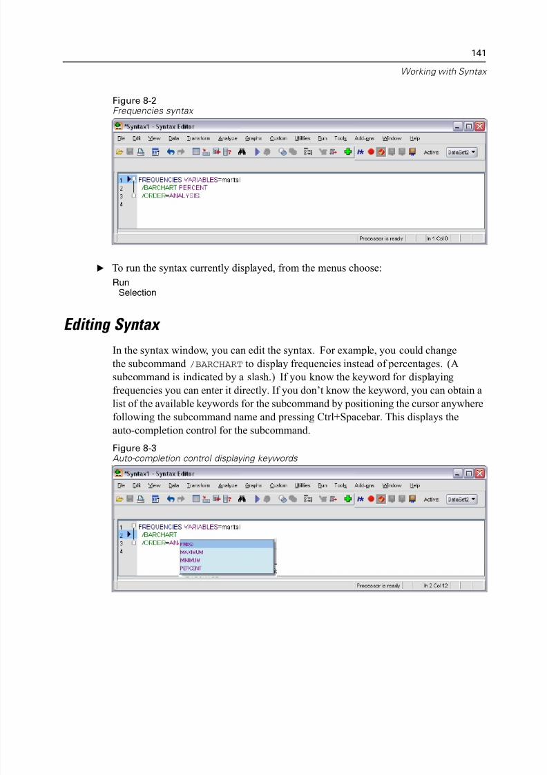
5/11/2018 SPSS Statistics Brief Guide 17.0 - slidepdf.com
http://slidepdf.com/reader/full/spss-statistics-brief-guide-170-55a2339b08a28 155/224
Working with Syn
Figure 8-2Frequencies syntax
E To run the syntax currently displayed, from the menus choose:Run
Selection
Editing Syntax
In the syntax window, you can edit the syntax. For example, you could change
the subcommand /BARCHART to display frequencies instead of percentages. (A
subcommand is indicated by a slash.) If you know the keyword for displaying
frequencies you can enter it directly. If you don’t know the keyword, you can obtain
list of the available keywords for the subcommand by positioning the cursor anywhfollowing the subcommand name and pressing Ctrl+Spacebar. This displays the
auto-completion control for the subcommand.
Figure 8-3Auto-completion control displaying keywords
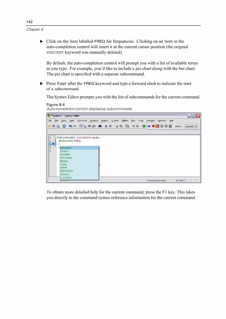
5/11/2018 SPSS Statistics Brief Guide 17.0 - slidepdf.com
http://slidepdf.com/reader/full/spss-statistics-brief-guide-170-55a2339b08a28 156/224
142
Chapter 8
E Click on the item labelled FREQ for frequencies. Clicking on an item in the
auto-completion control will insert it at the current cursor position (the original
PERCENT keyword was manually deleted).
By default, the auto-completion control will prompt you with a list of available term
as you type. For example, you’d like to include a pie chart along with the bar chart
The pie chart is specified with a separate subcommand.
E Press Enter after the FREQ keyword and type a forward slash to indicate the start
of a subcommand.
The Syntax Editor prompts you with the list of subcommands for the current comma
Figure 8-4Auto-completion control displaying subcommands
To obtain more detailed help for the current command, press the F1 key. This takes
you directly to the command syntax reference information for the current command
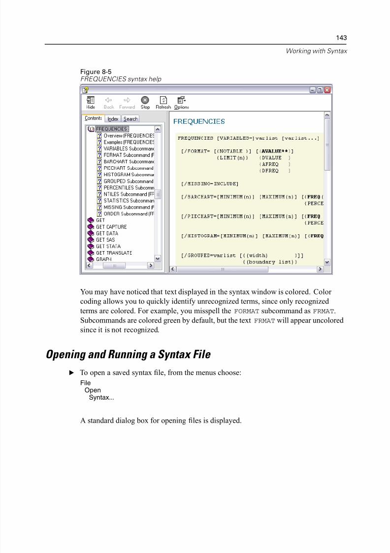
5/11/2018 SPSS Statistics Brief Guide 17.0 - slidepdf.com
http://slidepdf.com/reader/full/spss-statistics-brief-guide-170-55a2339b08a28 157/224
Working with Syn
Figure 8-5FREQUENCIES syntax help
You may have noticed that text displayed in the syntax window is colored. Color coding allows you to quickly identify unrecognized terms, since only recognized
terms are colored. For example, you misspell the FORMAT subcommand as FRMAT.
Subcommands are colored green by default, but the text FRMAT will appear uncolor
since it is not recognized.
Opening and Running a Syntax File
E To open a saved syntax file, from the menus choose:
FileOpenSyntax...
A standard dialog box for opening files is displayed.
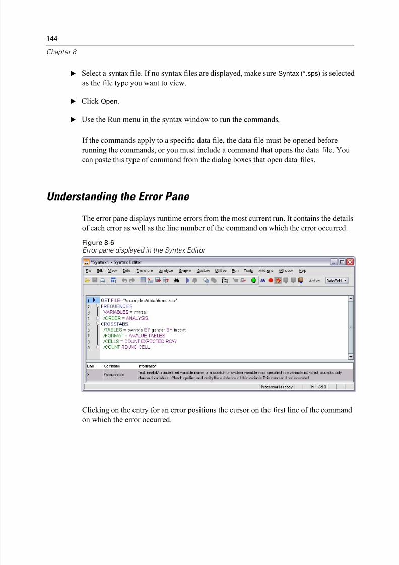
5/11/2018 SPSS Statistics Brief Guide 17.0 - slidepdf.com
http://slidepdf.com/reader/full/spss-statistics-brief-guide-170-55a2339b08a28 158/224
144
Chapter 8
E Select a syntax file. If no syntax files are displayed, make sure Syntax (*.sps) is selec
as the file type you want to view.
E Click Open.
E Use the Run menu in the syntax window to run the commands.
If the commands apply to a specific data file, the data file must be opened before
running the commands, or you must include a command that opens the data file. Yo
can paste this type of command from the dialog boxes that open data files.
Understanding the Error Pane
The error pane displays runtime errors from the most current run. It contains the det
of each error as well as the line number of the command on which the error occurred
Figure 8-6Error pane displayed in the Syntax Editor
Clicking on the entry for an error positions the cursor on the first line of the comma
on which the error occurred.
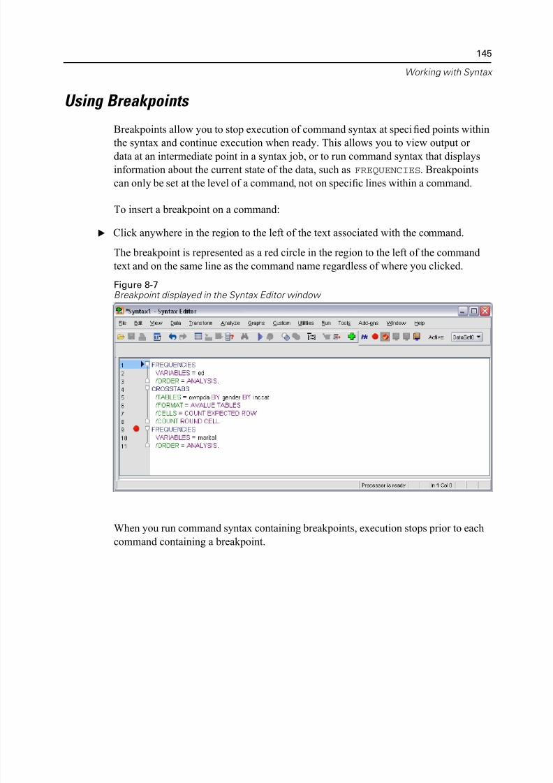
5/11/2018 SPSS Statistics Brief Guide 17.0 - slidepdf.com
http://slidepdf.com/reader/full/spss-statistics-brief-guide-170-55a2339b08a28 159/224
Working with Syn
Using Breakpoints
Breakpoints allow you to stop execution of command syntax at specified points wit
the syntax and continue execution when ready. This allows you to view output or
data at an intermediate point in a syntax job, or to run command syntax that display
information about the current state of the data, such as FREQUENCIES. Breakpoints
can only be set at the level of a command, not on specific lines within a command.
To insert a breakpoint on a command:
E Click anywhere in the region to the left of the text associated with the command.
The breakpoint is represented as a red circle in the region to the left of the comman
text and on the same line as the command name regardless of where you clicked.
Figure 8-7Breakpoint displayed in the Syntax Editor window
When you run command syntax containing breakpoints, execution stops prior to eac
command containing a breakpoint.
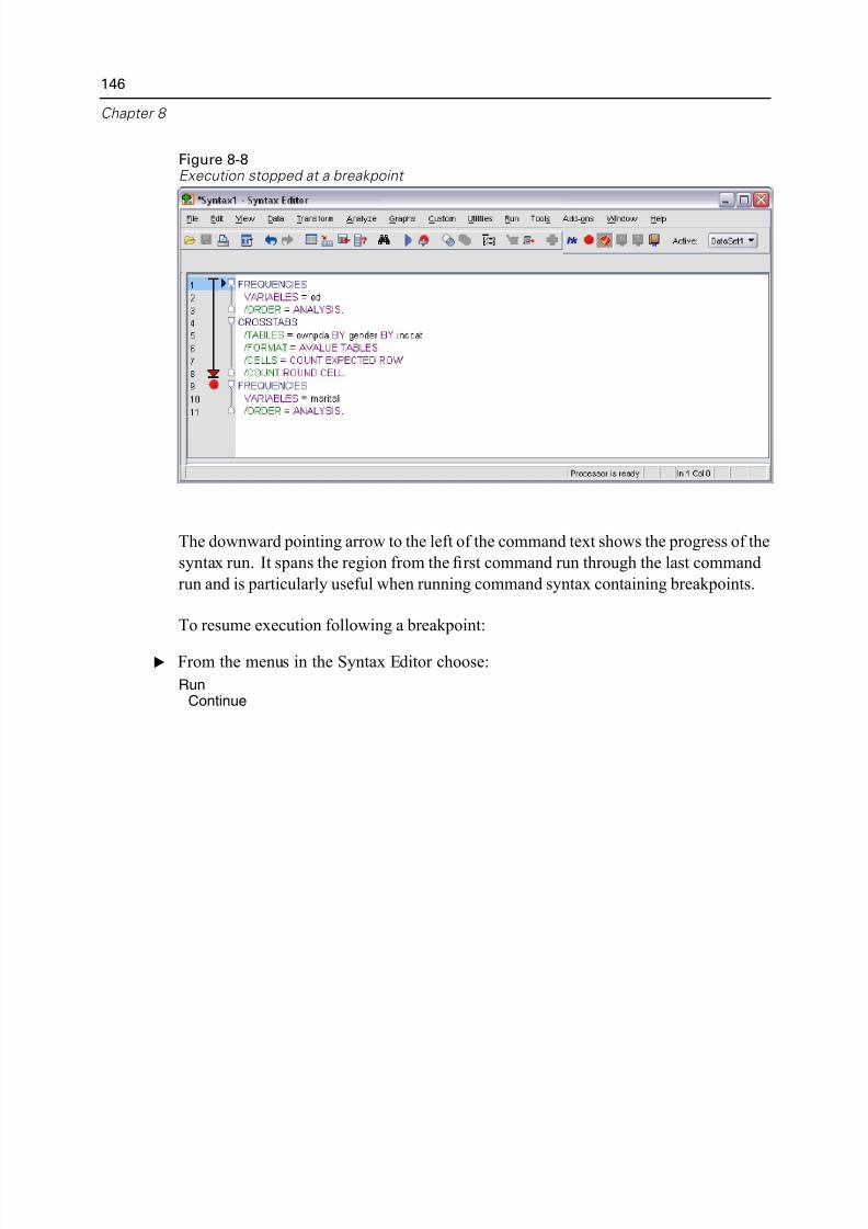
5/11/2018 SPSS Statistics Brief Guide 17.0 - slidepdf.com
http://slidepdf.com/reader/full/spss-statistics-brief-guide-170-55a2339b08a28 160/224
146
Chapter 8
Figure 8-8Execution stopped at a breakpoint
The downward pointing arrow to the left of the command text shows the progress of
syntax run. It spans the region from the first command run through the last comman
run and is particularly useful when running command syntax containing breakpoints
To resume execution following a breakpoint:
E From the menus in the Syntax Editor choose:
RunContinue
5/11/2018 SPSS Statistics Brief Guide 17.0 - slidepdf.com
http://slidepdf.com/reader/full/spss-statistics-brief-guide-170-55a2339b08a28 161/224
Chapt
9
Modifying Data Values
The data you start with may not always be organized in the most useful manner for
your analysis or reporting needs. For example, you may want to:
Create a categorical variable from a scale variable.
Combine several response categories into a single category.
Create a new variable that is the computed difference between two existing
variables.
Calculate the length of time between two dates.
This chapter uses the data file demo.sav. For more information, see Sample Files in
Appendix A on p. 194.
Creating a Categorical Variable from a Scale Variable
Several categorical variables in the data file demo.sav are, in fact, derived from sca
variables in that data file. For example, the variable inccat is simply income groupe
into four categories. This categorical variable uses the integer values 1–4 to represe
the following income categories (in thousands): less than $25, $25–$49, $50–$74,
and $75 or higher.
To create the categorical variable inccat :
E From the menus in the Data Editor window choose:
TransformVisual Binning...
147
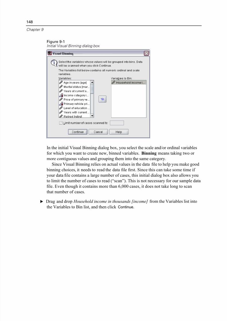
5/11/2018 SPSS Statistics Brief Guide 17.0 - slidepdf.com
http://slidepdf.com/reader/full/spss-statistics-brief-guide-170-55a2339b08a28 162/224
148
Chapter 9
Figure 9-1Initial Visual Binning dialog box
In the initial Visual Binning dialog box, you select the scale and/or ordinal variable
for which you want to create new, binned variables. Binning means taking two or
more contiguous values and grouping them into the same category.
Since Visual Binning relies on actual values in the data file to help you make goo
binning choices, it needs to read the data file first. Since this can take some time if
your data file contains a large number of cases, this initial dialog box also allows yo
to limit the number of cases to read (“scan”). This is not necessary for our sample d
file. Even though it contains more than 6,000 cases, it does not take long to scan
that number of cases.
E Drag and drop Household income in thousands [income] from the Variables list into
the Variables to Bin list, and then click Continue.
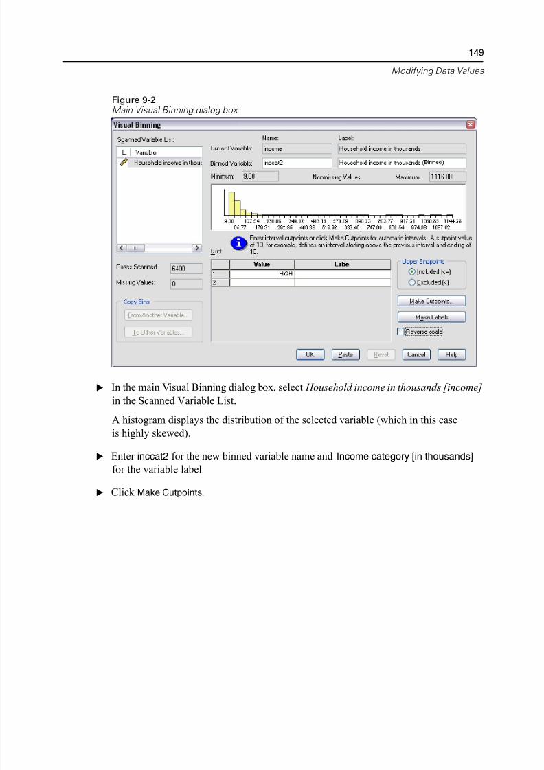
5/11/2018 SPSS Statistics Brief Guide 17.0 - slidepdf.com
http://slidepdf.com/reader/full/spss-statistics-brief-guide-170-55a2339b08a28 163/224
Modifying Data Val
Figure 9-2Main Visual Binning dialog box
E In the main Visual Binning dialog box, select Household income in thousands [incom
in the Scanned Variable List.A histogram displays the distribution of the selected variable (which in this case
is highly skewed).
E Enter inccat2 for the new binned variable name and Income category [in thousands
for the variable label.
E Click Make Cutpoints.
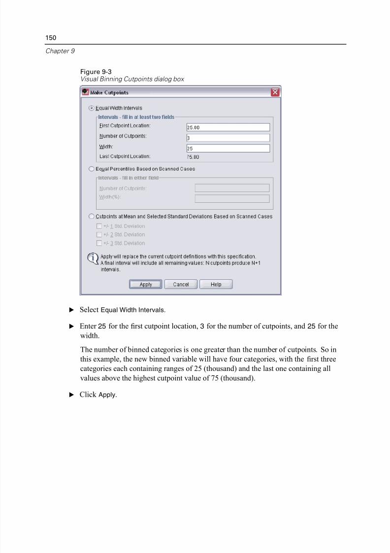
5/11/2018 SPSS Statistics Brief Guide 17.0 - slidepdf.com
http://slidepdf.com/reader/full/spss-statistics-brief-guide-170-55a2339b08a28 164/224
150
Chapter 9
Figure 9-3Visual Binning Cutpoints dialog box
E Select Equal Width Intervals.
E Enter 25 for the first cutpoint location, 3 for the number of cutpoints, and 25 for the
width.
The number of binned categories is one greater than the number of cutpoints. So in
this example, the new binned variable will have four categories, with the first three
categories each containing ranges of 25 (thousand) and the last one containing all
values above the highest cutpoint value of 75 (thousand).
E Click Apply.
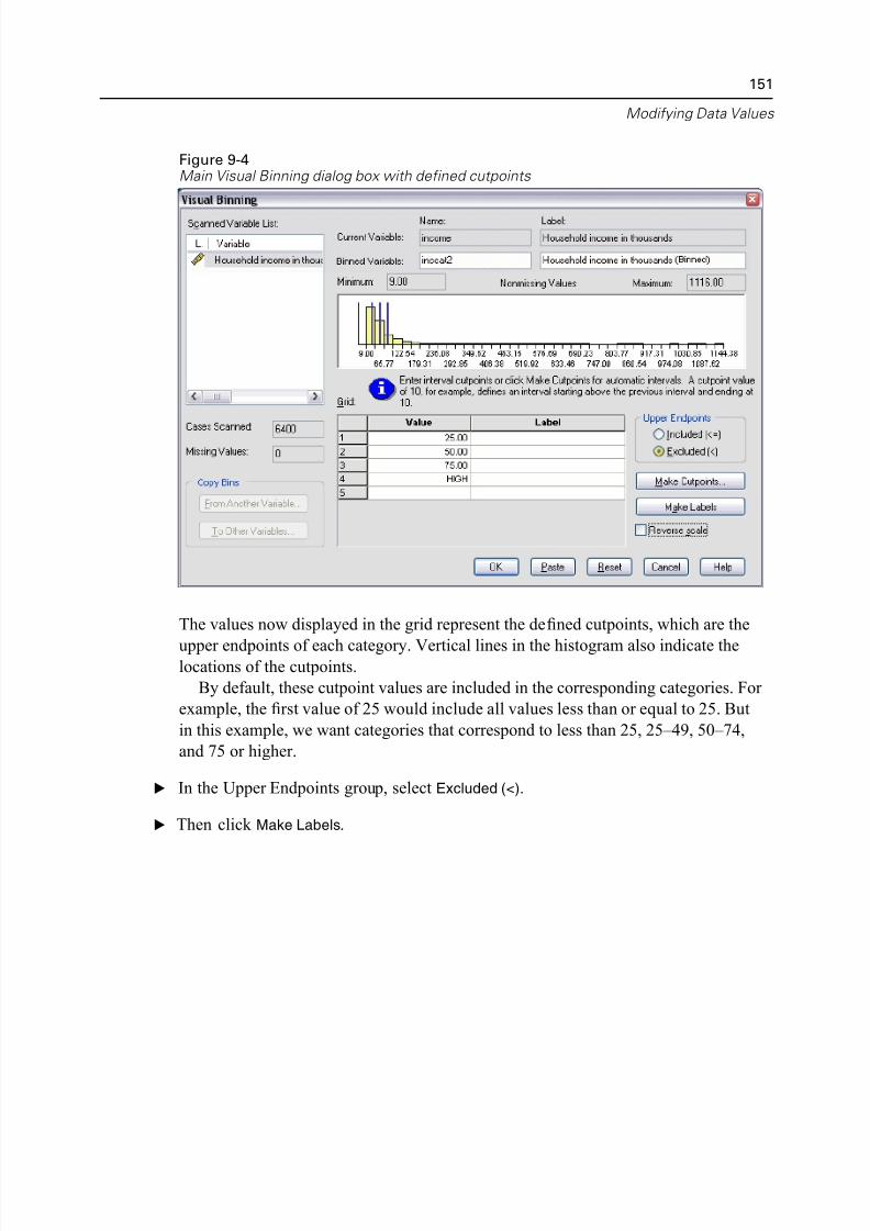
5/11/2018 SPSS Statistics Brief Guide 17.0 - slidepdf.com
http://slidepdf.com/reader/full/spss-statistics-brief-guide-170-55a2339b08a28 165/224
Modifying Data Val
Figure 9-4Main Visual Binning dialog box with defined cutpoints
The values now displayed in the grid represent the defined cutpoints, which are the
upper endpoints of each category. Vertical lines in the histogram also indicate thelocations of the cutpoints.
By default, these cutpoint values are included in the corresponding categories. F
example, the first value of 25 would include all values less than or equal to 25. But
in this example, we want categories that correspond to less than 25, 25–49, 50–74,
and 75 or higher.
E In the Upper Endpoints group, select Excluded (<).
E Then click Make Labels.
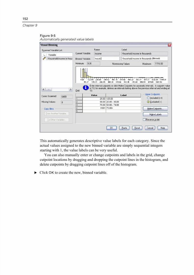
5/11/2018 SPSS Statistics Brief Guide 17.0 - slidepdf.com
http://slidepdf.com/reader/full/spss-statistics-brief-guide-170-55a2339b08a28 166/224
152
Chapter 9
Figure 9-5Automatically generated value labels
This automatically generates descriptive value labels for each category. Since the
actual values assigned to the new binned variable are simply sequential integers
starting with 1, the value labels can be very useful.
You can also manually enter or change cutpoints and labels in the grid, change
cutpoint locations by dragging and dropping the cutpoint lines in the histogram, and
delete cutpoints by dragging cutpoint lines off of the histogram.
E Click OK to create the new, binned variable.
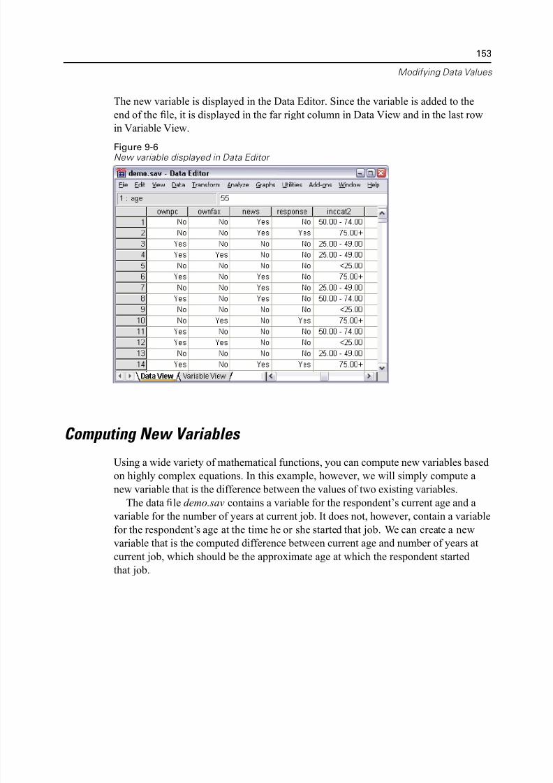
5/11/2018 SPSS Statistics Brief Guide 17.0 - slidepdf.com
http://slidepdf.com/reader/full/spss-statistics-brief-guide-170-55a2339b08a28 167/224
Modifying Data Val
The new variable is displayed in the Data Editor. Since the variable is added to the
end of the file, it is displayed in the far right column in Data View and in the last ro
in Variable View.
Figure 9-6New variable displayed in Data Editor
Computing New Variables
Using a wide variety of mathematical functions, you can compute new variables ba
on highly complex equations. In this example, however, we will simply compute a
new variable that is the difference between the values of two existing variables.
The data file demo.sav contains a variable for the respondent’s current age and a
variable for the number of years at current job. It does not, however, contain a varia
for the respondent’s age at the time he or she started that job. We can create a new
variable that is the computed difference between current age and number of years acurrent job, which should be the approximate age at which the respondent started
that job.
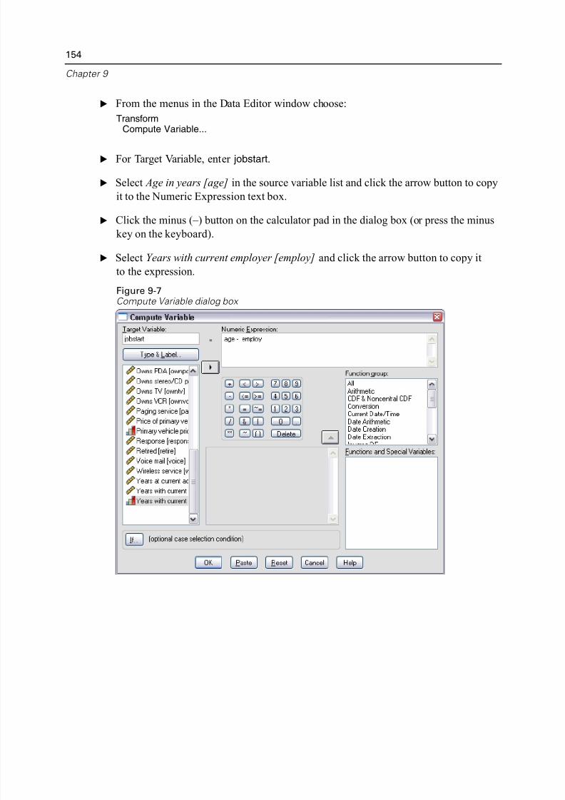
5/11/2018 SPSS Statistics Brief Guide 17.0 - slidepdf.com
http://slidepdf.com/reader/full/spss-statistics-brief-guide-170-55a2339b08a28 168/224
154
Chapter 9
E From the menus in the Data Editor window choose:
TransformCompute Variable...
E For Target Variable, enter jobstart.
E Select Age in years [age] in the source variable list and click the arrow button to co
it to the Numeric Expression text box.
E Click the minus (–) button on the calculator pad in the dialog box (or press the minu
key on the keyboard).
E Select Years with current employer [employ] and click the arrow button to copy it
to the expression.
Figure 9-7Compute Variable dialog box
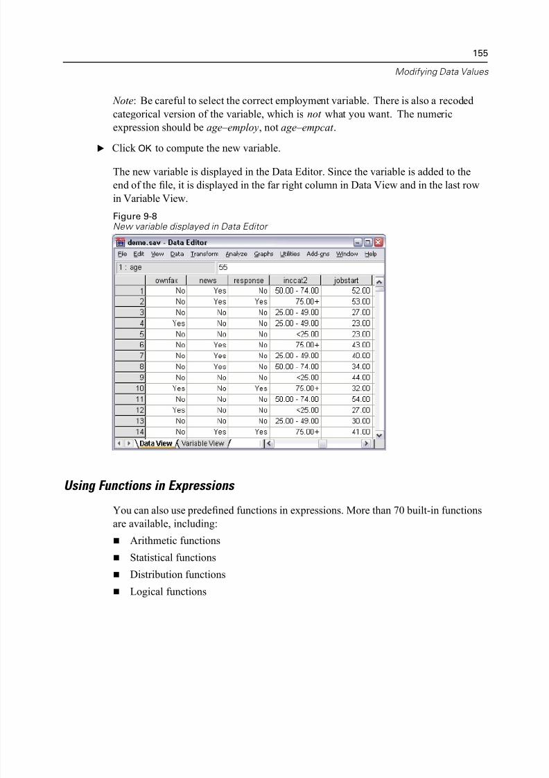
5/11/2018 SPSS Statistics Brief Guide 17.0 - slidepdf.com
http://slidepdf.com/reader/full/spss-statistics-brief-guide-170-55a2339b08a28 169/224
Modifying Data Val
Note: Be careful to select the correct employment variable. There is also a recoded
categorical version of the variable, which is not what you want. The numeric
expression should be age–employ, not age–empcat .
E Click OK to compute the new variable.
The new variable is displayed in the Data Editor. Since the variable is added to the
end of the file, it is displayed in the far right column in Data View and in the last ro
in Variable View.
Figure 9-8New variable displayed in Data Editor
Using Functions in Expressions
You can also use predefined functions in expressions. More than 70 built-in functio
are available, including:
Arithmetic functions Statistical functions
Distribution functions
Logical functions
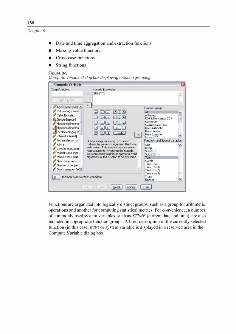
5/11/2018 SPSS Statistics Brief Guide 17.0 - slidepdf.com
http://slidepdf.com/reader/full/spss-statistics-brief-guide-170-55a2339b08a28 170/224
156
Chapter 9
Date and time aggregation and extraction functions
Missing-value functions
Cross-case functions String functions
Figure 9-9Compute Variable dialog box displaying function grouping
Functions are organized into logically distinct groups, such as a group for arithmeti
operations and another for computing statistical metrics. For convenience, a numbe
of commonly used system variables, such as $TIME (current date and time), are als
included in appropriate function groups. A brief description of the currently selecte
function (in this case, SUM) or system variable is displayed in a reserved area in the
Compute Variable dialog box.
5/11/2018 SPSS Statistics Brief Guide 17.0 - slidepdf.com
http://slidepdf.com/reader/full/spss-statistics-brief-guide-170-55a2339b08a28 171/224
Modifying Data Val
Pasting a Function into an Expression
To paste a function into an expression:
E Position the cursor in the expression at the point where you want the function to appe
E Select the appropriate group from the Function group list. The group labeled All
provides a listing of all available functions and system variables.
E Double-click the function in the Functions and Special Variables list (or select the
function and click the arrow adjacent to the Function group list).
The function is inserted into the expression. If you highlight part of the expression
and then insert the function, the highlighted portion of the expression is used as the
first argument in the function.
Editing a Function in an Expression
The function is not complete until you enter the arguments, represented by question
marks in the pasted function. The number of question marks indicates the minimum
number of arguments required to complete the function.
E Highlight the question mark(s) in the pasted function.
E Enter the arguments. If the arguments are variable names, you can paste them from
the variable list.
Using Conditional Expressions
You can use conditional expressions (also called logical expressions) to apply
transformations to selected subsets of cases. A conditional expression returns a valu
of true, false, or missing for each case. If the result of a conditional expression is
true, the transformation is applied to that case. If the result is false or missing, the
transformation is not applied to the case.
To specify a conditional expression:
E Click If in the Compute Variable dialog box. This opens the If Cases dialog box.
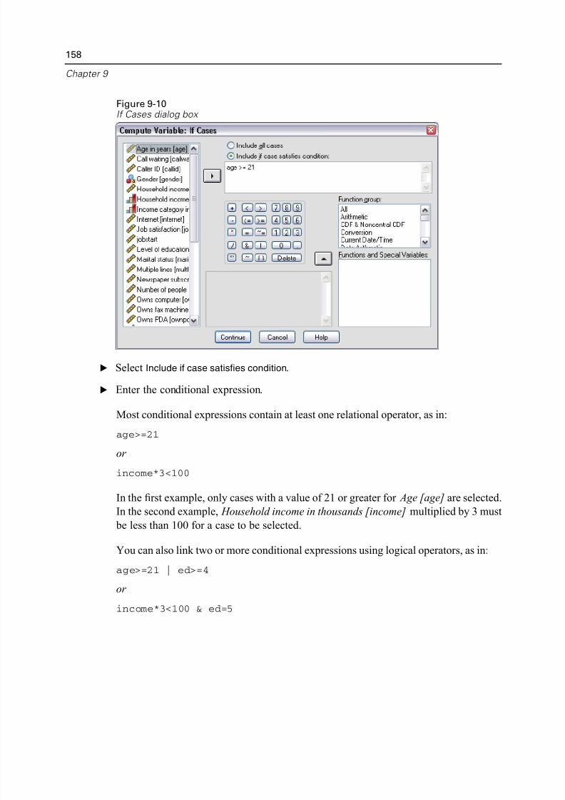
5/11/2018 SPSS Statistics Brief Guide 17.0 - slidepdf.com
http://slidepdf.com/reader/full/spss-statistics-brief-guide-170-55a2339b08a28 172/224
158
Chapter 9
Figure 9-10If Cases dialog box
E Select Include if case satisfies condition.
E Enter the conditional expression.
Most conditional expressions contain at least one relational operator, as in:age>=21
or
income*3<100
In the first example, only cases with a value of 21 or greater for Age [age] are select
In the second example, Household income in thousands [income] multiplied by 3 m
be less than 100 for a case to be selected.
You can also link two or more conditional expressions using logical operators, as in
age>=21 | ed>=4
or
income*3<100 & ed=5
5/11/2018 SPSS Statistics Brief Guide 17.0 - slidepdf.com
http://slidepdf.com/reader/full/spss-statistics-brief-guide-170-55a2339b08a28 173/224
Modifying Data Val
In the first example, cases that meet either the Age [age] condition or the Level of
education [ed] condition are selected. In the second example, both the Household
income in thousands [income] and Level of education [ed] conditions must be met
for a case to be selected.
Working with Dates and Times
A number of tasks commonly performed with dates and times can be easily
accomplished using the Date and Time Wizard. Using this wizard, you can:
Create a date/time variable from a string variable containing a date or time.
Construct a date/time variable by merging variables containing different parts o
the date or time.
Add or subtract values from date/time variables, including adding or subtractin
two date/time variables.
Extract a part of a date or time variable; for example, the day of month from a
date/time variable which has the form mm/dd/yyyy.
The examples in this section use the data file upgrade.sav. For more information, s
Sample Files in Appendix A on p. 194.
To use the Date and Time Wizard:
E From the menus choose:Transform
Date and Time Wizard...
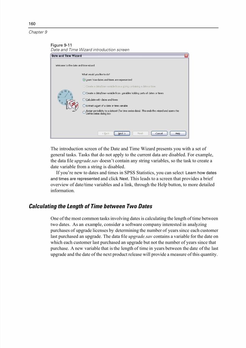
5/11/2018 SPSS Statistics Brief Guide 17.0 - slidepdf.com
http://slidepdf.com/reader/full/spss-statistics-brief-guide-170-55a2339b08a28 174/224
160
Chapter 9
Figure 9-11Date and Time Wizard introduction screen
The introduction screen of the Date and Time Wizard presents you with a set of
general tasks. Tasks that do not apply to the current data are disabled. For example
the data file upgrade.sav doesn’t contain any string variables, so the task to create a
date variable from a string is disabled.
If you’re new to dates and times in SPSS Statistics, you can select Learn how dat
and times are represented and click Next. This leads to a screen that provides a brief
overview of date/time variables and a link, through the Help button, to more detaile
information.
Calculating the Length of Time between Two Dates
One of the most common tasks involving dates is calculating the length of time betw
two dates. As an example, consider a software company interested in analyzing
purchases of upgrade licenses by determining the number of years since each custom
last purchased an upgrade. The data file upgrade.sav contains a variable for the date
which each customer last purchased an upgrade but not the number of years since th purchase. A new variable that is the length of time in years between the date of the
upgrade and the date of the next product release will provide a measure of this quant
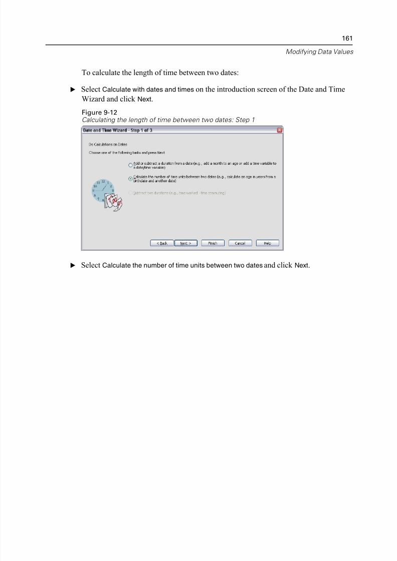
5/11/2018 SPSS Statistics Brief Guide 17.0 - slidepdf.com
http://slidepdf.com/reader/full/spss-statistics-brief-guide-170-55a2339b08a28 175/224
Modifying Data Val
To calculate the length of time between two dates:
E Select Calculate with dates and times on the introduction screen of the Date and Tim
Wizard and click Next.
Figure 9-12Calculating the length of time between two dates: Step 1
E Select Calculate the number of time units between two dates and click Next.
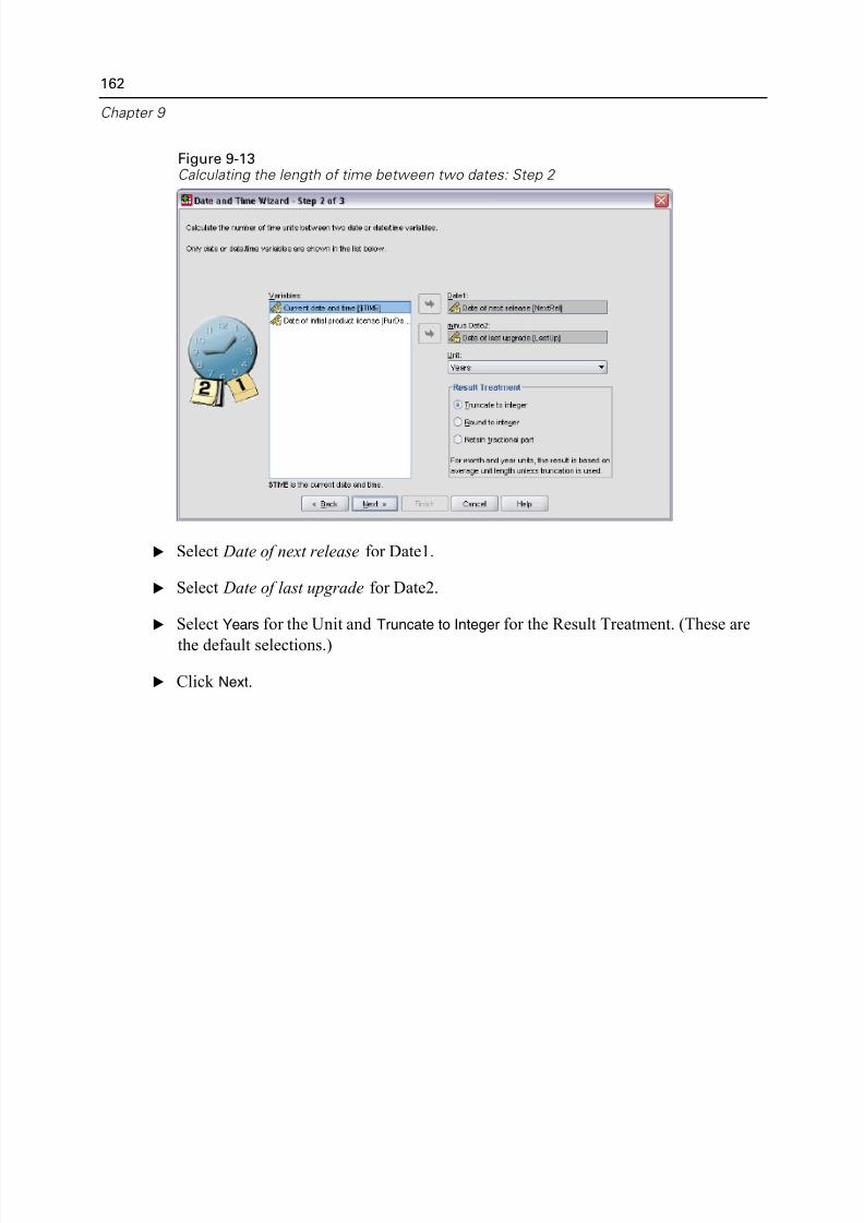
5/11/2018 SPSS Statistics Brief Guide 17.0 - slidepdf.com
http://slidepdf.com/reader/full/spss-statistics-brief-guide-170-55a2339b08a28 176/224
162
Chapter 9
Figure 9-13Calculating the length of time between two dates: Step 2
E Select Date of next release for Date1.
E Select Date of last upgrade for Date2.
E Select Years for the Unit and Truncate to Integer for the Result Treatment. (These ar
the default selections.)
E Click Next.
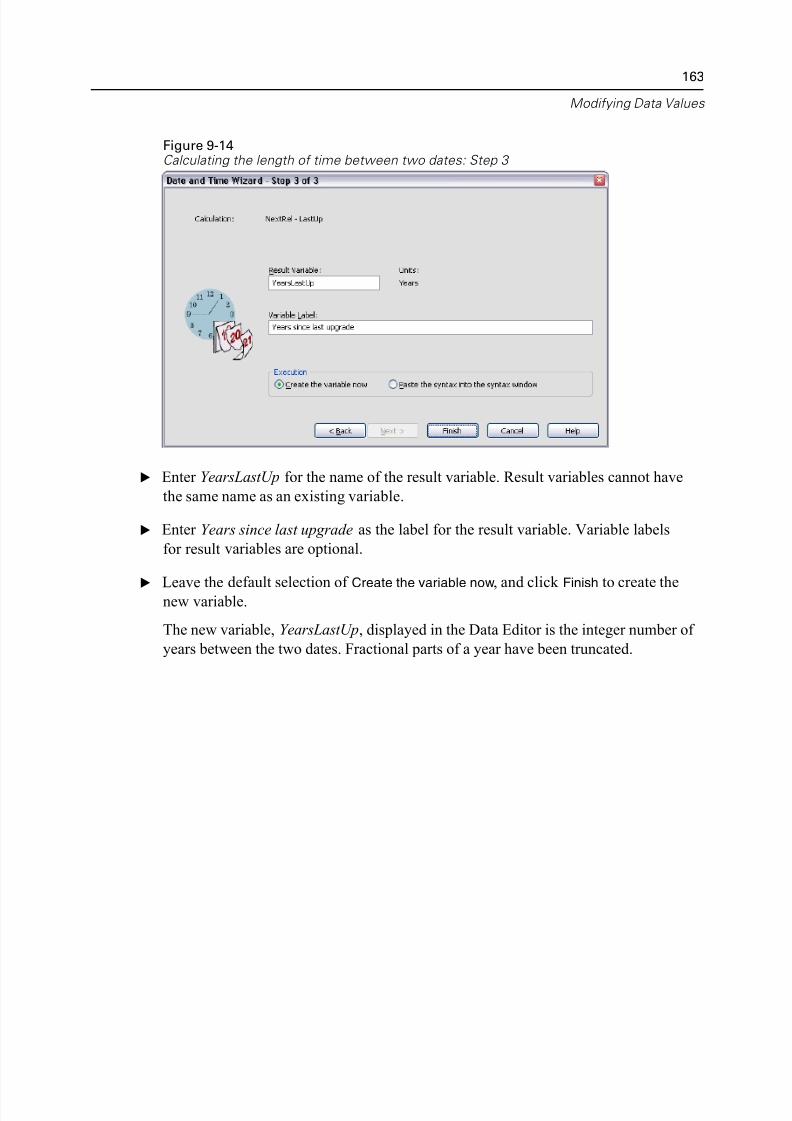
5/11/2018 SPSS Statistics Brief Guide 17.0 - slidepdf.com
http://slidepdf.com/reader/full/spss-statistics-brief-guide-170-55a2339b08a28 177/224
Modifying Data Val
Figure 9-14Calculating the length of time between two dates: Step 3
E Enter YearsLastUp for the name of the result variable. Result variables cannot have
the same name as an existing variable.
E Enter Years since last upgrade as the label for the result variable. Variable labels
for result variables are optional.
E Leave the default selection of Create the variable now, and click Finish to create thenew variable.
The new variable, YearsLastUp, displayed in the Data Editor is the integer number
years between the two dates. Fractional parts of a year have been truncated.
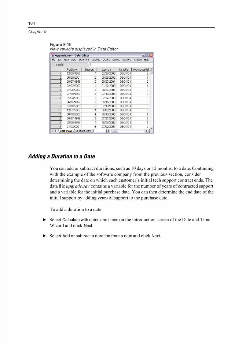
5/11/2018 SPSS Statistics Brief Guide 17.0 - slidepdf.com
http://slidepdf.com/reader/full/spss-statistics-brief-guide-170-55a2339b08a28 178/224
164
Chapter 9
Figure 9-15New variable displayed in Data Editor
Adding a Duration to a Date
You can add or subtract durations, such as 10 days or 12 months, to a date. Continui
with the example of the software company from the previous section, consider
determining the date on which each customer’s initial tech support contract ends. Tdata file upgrade.sav contains a variable for the number of years of contracted supp
and a variable for the initial purchase date. You can then determine the end date of
initial support by adding years of support to the purchase date.
To add a duration to a date:
E Select Calculate with dates and times on the introduction screen of the Date and Tim
Wizard and click Next.
E Select Add or subtract a duration from a date and click Next.
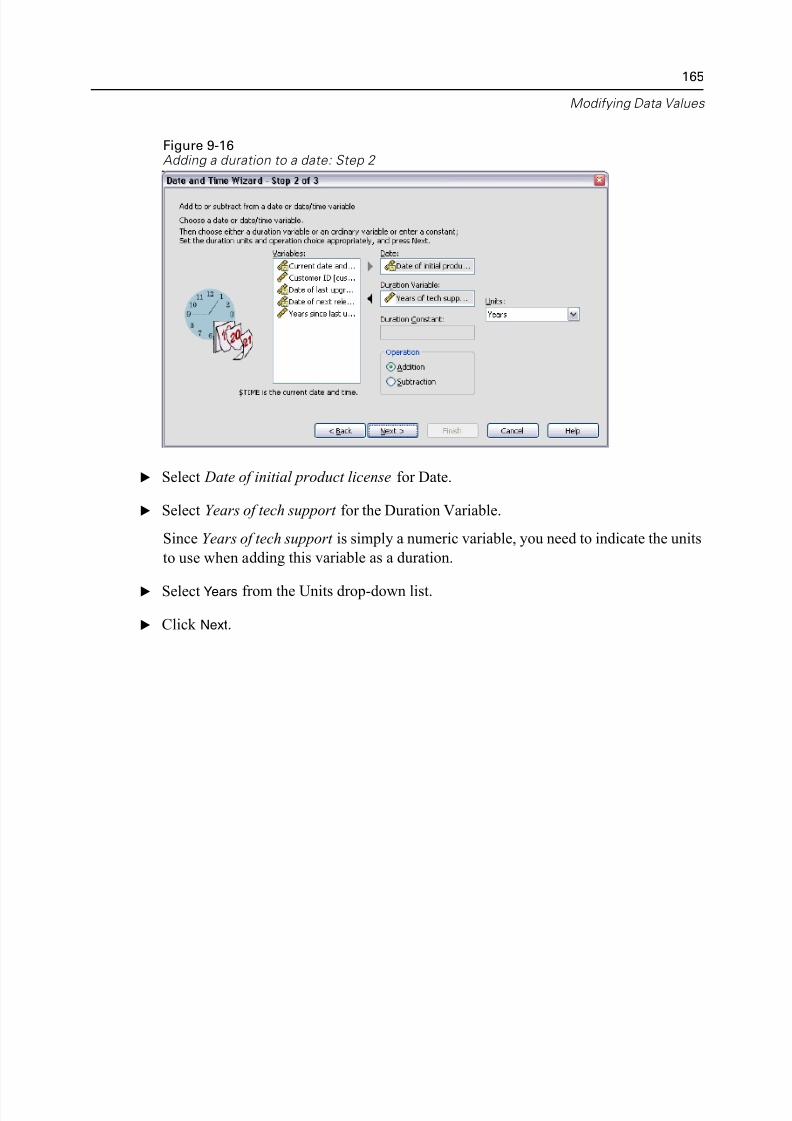
5/11/2018 SPSS Statistics Brief Guide 17.0 - slidepdf.com
http://slidepdf.com/reader/full/spss-statistics-brief-guide-170-55a2339b08a28 179/224
Modifying Data Val
Figure 9-16Adding a duration to a date: Step 2
E Select Date of initial product license for Date.
E Select Years of tech support for the Duration Variable.
Since Years of tech support is simply a numeric variable, you need to indicate the un
to use when adding this variable as a duration.
E Select Years from the Units drop-down list.
E Click Next.
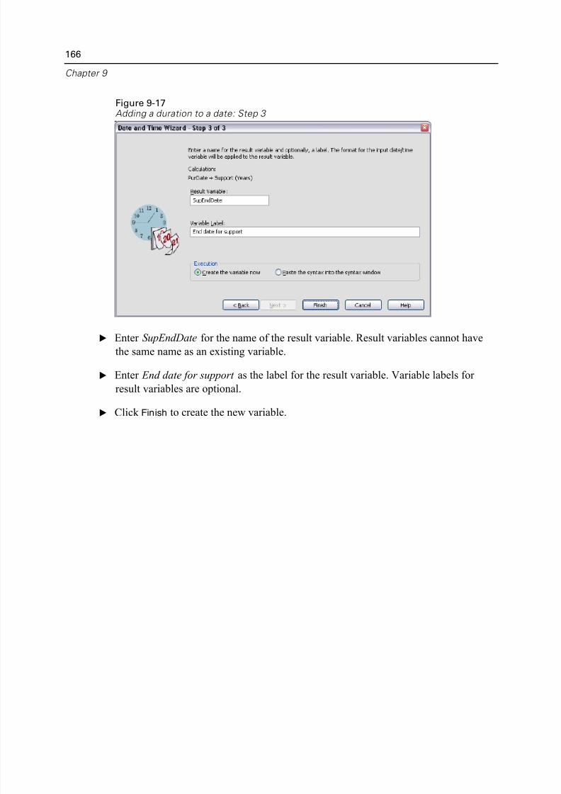
5/11/2018 SPSS Statistics Brief Guide 17.0 - slidepdf.com
http://slidepdf.com/reader/full/spss-statistics-brief-guide-170-55a2339b08a28 180/224
166
Chapter 9
Figure 9-17Adding a duration to a date: Step 3
E Enter SupEndDate for the name of the result variable. Result variables cannot have
the same name as an existing variable.
E Enter End date for support as the label for the result variable. Variable labels for
result var iables are optional.
E Click Finish to create the new variable.
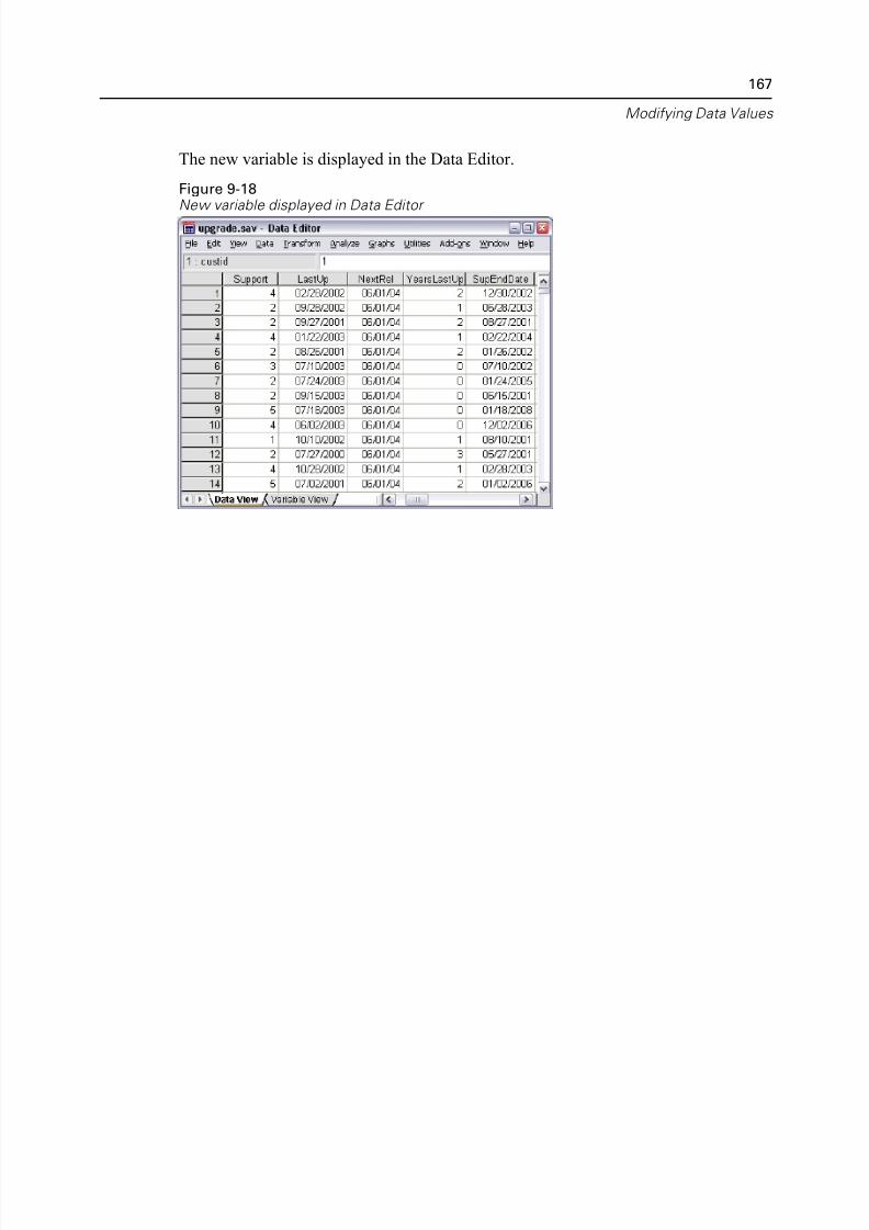
5/11/2018 SPSS Statistics Brief Guide 17.0 - slidepdf.com
http://slidepdf.com/reader/full/spss-statistics-brief-guide-170-55a2339b08a28 181/224
Modifying Data Val
The new variable is displayed in the Data Editor.
Figure 9-18New variable displayed in Data Editor
5/11/2018 SPSS Statistics Brief Guide 17.0 - slidepdf.com
http://slidepdf.com/reader/full/spss-statistics-brief-guide-170-55a2339b08a28 182/224
Chapt
10
Sorting and Selecting Data
Data files are not always organized in the ideal form for your specific needs. To
prepare data for analysis, you can select from a wide range of file transformations,
including the ability to:
Sort data. You can sort cases based on the value of one or more variables.
Select subsets of cases. You can restrict your analysis to a subset of cases or
perform simultaneous analyses on different subsets.
The examples in this chapter use the data file demo.sav. For more information, see
Sample Files in Appendix A on p. 194.
Sorting Data
Sorting cases (sorting rows of the data file) is often useful and sometimes necessary
certain types of analysis.
To reorder the sequence of cases in the data file based on the value of one or mor
sorting variables:
E From the menus choose:
DataSort Cases...
168
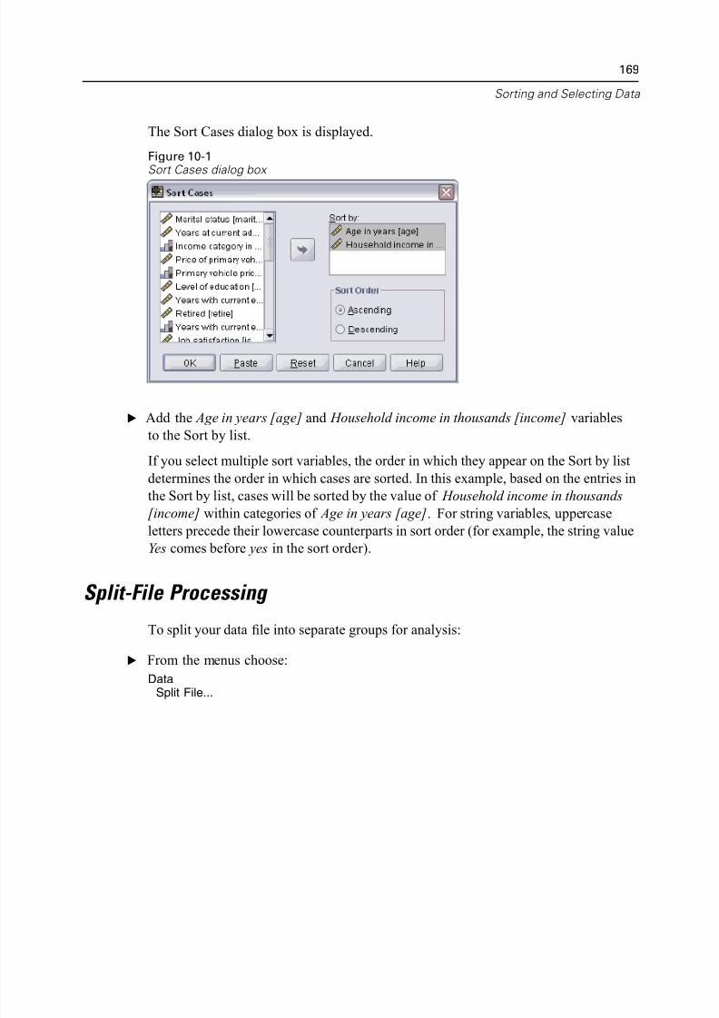
5/11/2018 SPSS Statistics Brief Guide 17.0 - slidepdf.com
http://slidepdf.com/reader/full/spss-statistics-brief-guide-170-55a2339b08a28 183/224
Sorting and Selecting D
The Sort Cases dialog box is displayed.
Figure 10-1Sort Cases dialog box
E Add the Age in years [age] and Household income in thousands [income] variables
to the Sort by list.
If you select multiple sort variables, the order in which they appear on the Sort by l
determines the order in which cases are sorted. In this example, based on the entries
the Sort by list, cases will be sorted by the value of Household income in thousands
[income] within categories of Age in years [age]. For string variables, uppercase
letters precede their lowercase counterparts in sort order (for example, the string valYes comes before yes in the sort order).
Split-File Processing
To split your data file into separate groups for analysis:
E From the menus choose:
DataSplit File...
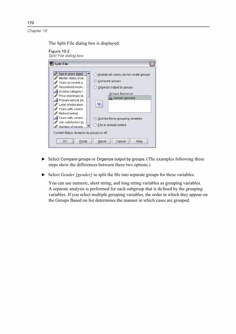
5/11/2018 SPSS Statistics Brief Guide 17.0 - slidepdf.com
http://slidepdf.com/reader/full/spss-statistics-brief-guide-170-55a2339b08a28 184/224
170
Chapter 10
The Split File dialog box is displayed.
Figure 10-2Split File dialog box
E Select Compare groups or Organize output by groups. (The examples following these
steps show the differences between these two options.)
E Select Gender [gender] to split the file into separate groups for these variables.
You can use numeric, short string, and long string variables as grouping variables.
A separate analysis is performed for each subgroup that is defined by the grouping
variables. If you select multiple grouping variables, the order in which they appear
the Groups Based on list determines the manner in which cases are grouped.
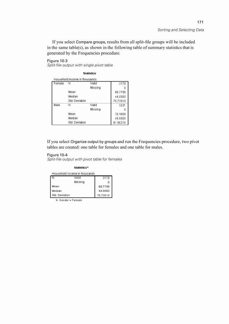
5/11/2018 SPSS Statistics Brief Guide 17.0 - slidepdf.com
http://slidepdf.com/reader/full/spss-statistics-brief-guide-170-55a2339b08a28 185/224
Sorting and Selecting D
If you select Compare groups, results from all split-file groups will be included
in the same table(s), as shown in the following table of summary statistics that is
generated by the Frequencies procedure.
Figure 10-3Split-file output with single pivot table
If you select Organize output by groups and run the Frequencies procedure, two pivo
tables are created: one table for females and one table for males.
Figure 10-4Split-file output with pivot table for females
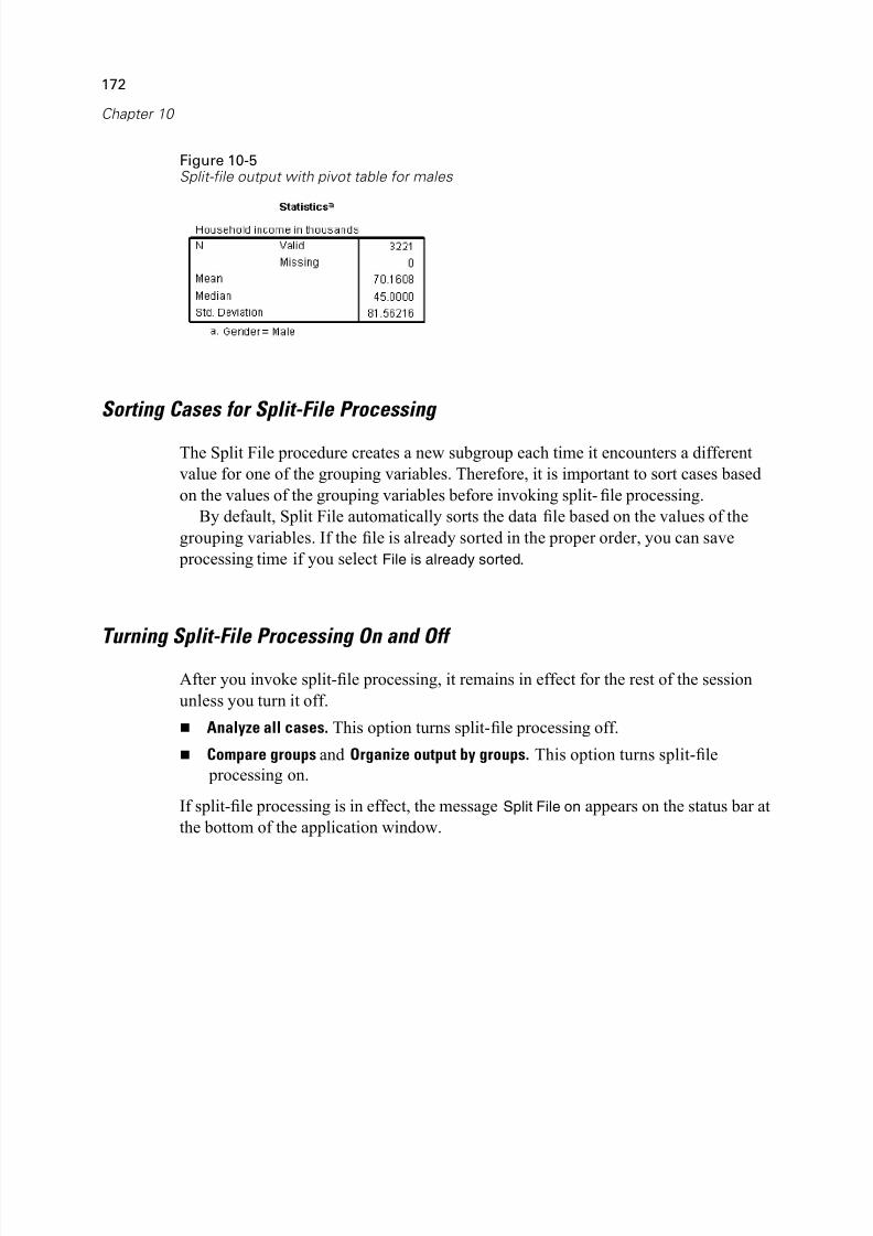
5/11/2018 SPSS Statistics Brief Guide 17.0 - slidepdf.com
http://slidepdf.com/reader/full/spss-statistics-brief-guide-170-55a2339b08a28 186/224
172
Chapter 10
Figure 10-5Split-file output with pivot table for males
Sorting Cases for Split-File Processing
The Split File procedure creates a new subgroup each time it encounters a different
value for one of the grouping variables. Therefore, it is important to sort cases base
on the values of the grouping variables before invoking split-file processing.
By default, Split File automatically sorts the data file based on the values of the
grouping variables. If the file is already sorted in the proper order, you can save
processing time if you select File is already sorted.
Turning Split-File Processing On and Off After you invoke split-file processing, it remains in effect for the rest of the session
unless you turn it off.
Analyze all cases. This option turns split-file processing off.
Compare groups and Organize output by groups. This option turns split-file
processing on.
If split-file processing is in effect, the message Split File on appears on the status bar
the bottom of the application window.
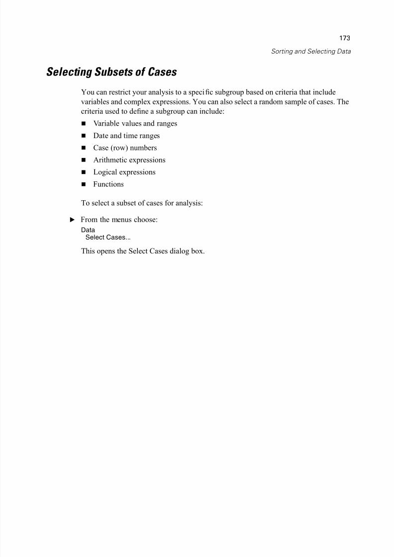
5/11/2018 SPSS Statistics Brief Guide 17.0 - slidepdf.com
http://slidepdf.com/reader/full/spss-statistics-brief-guide-170-55a2339b08a28 187/224
Sorting and Selecting D
Selecting Subsets of Cases
You can restrict your analysis to a specific subgroup based on criteria that include
variables and complex expressions. You can also select a random sample of cases. T
criteria used to define a subgroup can include:
Variable values and ranges
Date and time ranges
Case (row) numbers
Arithmetic expressions
Logical expressions
Functions
To select a subset of cases for analysis:
E From the menus choose:
DataSelect Cases...
This opens the Select Cases dialog box.
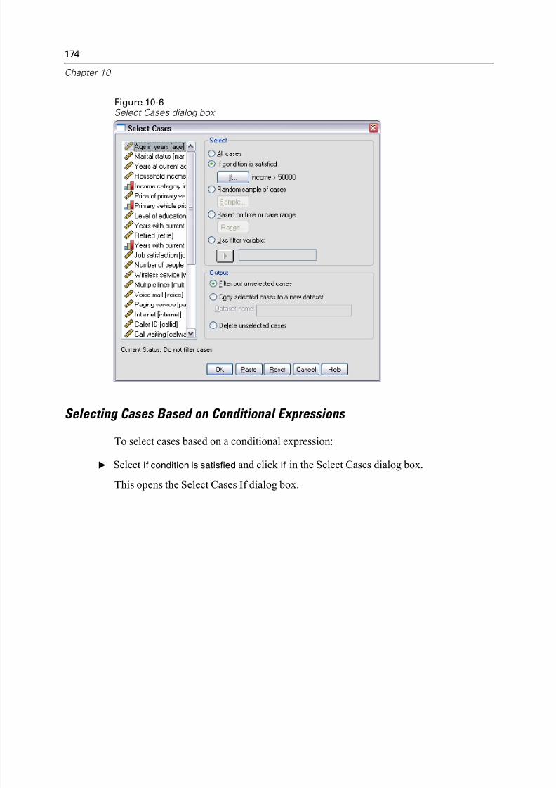
5/11/2018 SPSS Statistics Brief Guide 17.0 - slidepdf.com
http://slidepdf.com/reader/full/spss-statistics-brief-guide-170-55a2339b08a28 188/224
174
Chapter 10
Figure 10-6Select Cases dialog box
Selecting Cases Based on Conditional Expressions
To select cases based on a conditional expression:
E Select If condition is satisfied and click If in the Select Cases dialog box.
This opens the Select Cases If dialog box.
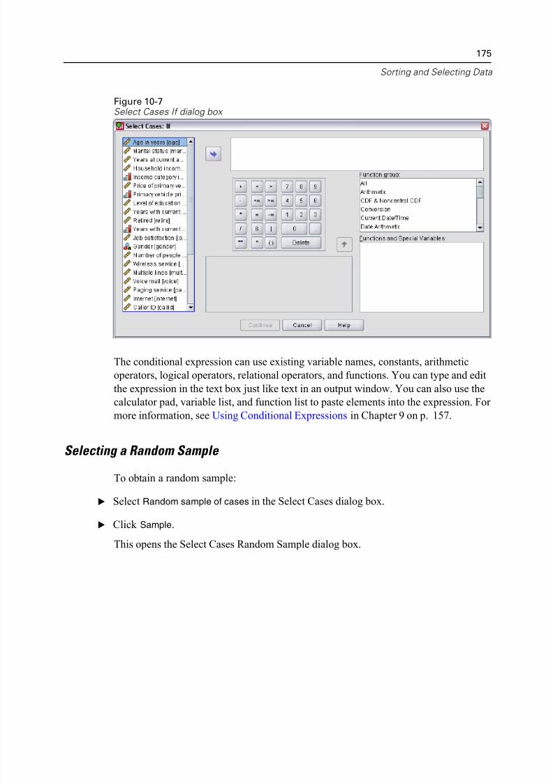
5/11/2018 SPSS Statistics Brief Guide 17.0 - slidepdf.com
http://slidepdf.com/reader/full/spss-statistics-brief-guide-170-55a2339b08a28 189/224
Sorting and Selecting D
Figure 10-7Select Cases If dialog box
The conditional expression can use existing variable names, constants, arithmetic
operators, logical operators, relational operators, and functions. You can type and e
the expression in the text box just like text in an output window. You can also use th
calculator pad, variable list, and function list to paste elements into the expression.
more information, see Using Conditional Expressions in Chapter 9 on p. 157.
Selecti ng a Random Sample
To obtain a random sample:
E Select Random sample of cases in the Select Cases dialog box.
E Click Sample.
This opens the Select Cases Random Sample dialog box.
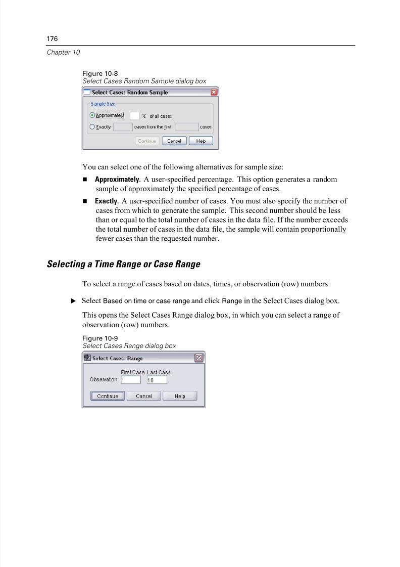
5/11/2018 SPSS Statistics Brief Guide 17.0 - slidepdf.com
http://slidepdf.com/reader/full/spss-statistics-brief-guide-170-55a2339b08a28 190/224
176
Chapter 10
Figure 10-8Select Cases Random Sample dialog box
You can select one of the following alternatives for sample size:
Approximately. A user-specified percentage. This option generates a random
sample of approximately the specified percentage of cases.
Exactly. A user-specified number of cases. You must also specify the number o
cases from which to generate the sample. This second number should be less
than or equal to the total number of cases in the data file. If the number exceed
the total number of cases in the data file, the sample will contain proportionally
fewer cases than the requested number.
Selecting a Time Range or Case Range
To select a range of cases based on dates, times, or observation (row) numbers:
E Select Based on time or case range and click Range in the Select Cases dialog box.
This opens the Select Cases Range dialog box, in which you can select a range of
observation (row) numbers.
Figure 10-9Select Cases Range dialog box
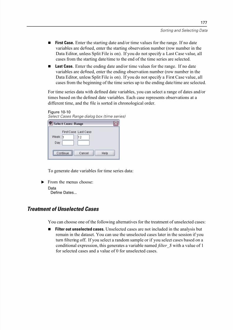
5/11/2018 SPSS Statistics Brief Guide 17.0 - slidepdf.com
http://slidepdf.com/reader/full/spss-statistics-brief-guide-170-55a2339b08a28 191/224
Sorting and Selecting D
First Case. Enter the starting date and/or time values for the range. If no date
variables are defined, enter the starting observation number (row number in the
Data Editor, unless Split File is on). If you do not specify a Last Case value, al
cases from the starting date/time to the end of the time series are selected.
Last Case. Enter the ending date and/or time values for the range. If no date
variables are defined, enter the ending observation number (row number in the
Data Editor, unless Split File is on). If you do not specify a First Case value, al
cases from the beginning of the time series up to the ending date/time are select
For time series data with defined date variables, you can select a range of dates and
times based on the defined date variables. Each case represents observations at a
different time, and the file is sorted in chronological order.
Figure 10-10
Select Cases Range dialog box (time series)
To generate date variables for time series data:
E From the menus choose:
DataDefine Dates...
Treatment of Unselected Cases
You can choose one of the following alternatives for the treatment of unselected cas
Filter out unselected cases. Unselected cases are not included in the analysis buremain in the dataset. You can use the unselected cases later in the session if yo
turn filtering off. If you select a random sample or if you select cases based on
conditional expression, this generates a variable named filter_$ with a value of
for selected cases and a value of 0 for unselected cases.
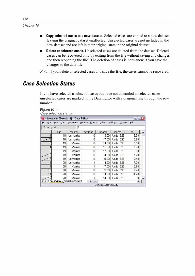
5/11/2018 SPSS Statistics Brief Guide 17.0 - slidepdf.com
http://slidepdf.com/reader/full/spss-statistics-brief-guide-170-55a2339b08a28 192/224
178
Chapter 10
Copy selected cases to a new dataset. Selected cases are copied to a new datase
leaving the original dataset unaffected. Unselected cases are not included in th
new dataset and are left in their original state in the original dataset.
Delete unselected cases. Unselected cases are deleted from the dataset. Deleted
cases can be recovered only by exiting from the file without saving any change
and then reopening the file. The deletion of cases is permanent if you save the
changes to the data file.
Note: If you delete unselected cases and save the file, the cases cannot be recovered
Case Selection Status
If you have selected a subset of cases but have not discarded unselected cases,
unselected cases are marked in the Data Editor with a diagonal line through the row
number.
Figure 10-11Case selection status
5/11/2018 SPSS Statistics Brief Guide 17.0 - slidepdf.com
http://slidepdf.com/reader/full/spss-statistics-brief-guide-170-55a2339b08a28 193/224
Chapt
11
Additional Statistical Procedures
This chapter contains brief examples for selected statistical procedures. The procedu
are grouped according to the order in which they appear on the Analyze menu.
The examples are designed to illustrate sample specifications that are required to
run a statistical procedure. The examples in this chapter use the data file demo.sav,
with the following exceptions: The paired-samples t test example uses the data file dietstudy.sav, which is a
hypothetical data file containing the results of a study of the “Stillman diet.” In
examples in this chapter, you must run the procedures to see the output.
The correlation examples use Employee data.sav, which contains historical data
about a company’s employees.
The exponential smoothing example uses the data file inventor.sav, which conta
inventory data that were collected over a period of 70 days.
For information about individual items in a dialog box, click Help. If you want to loc
a specific statistic, such as percentiles, use the Index or Search facility in the Help
system. For additional information about interpreting the results of these procedure
consult a statistics or data analysis textbook.
Summarizing Data
The Descriptive Statistics submenu on the Analyze menu provides techniques for
summarizing data with statistics and charts.
179
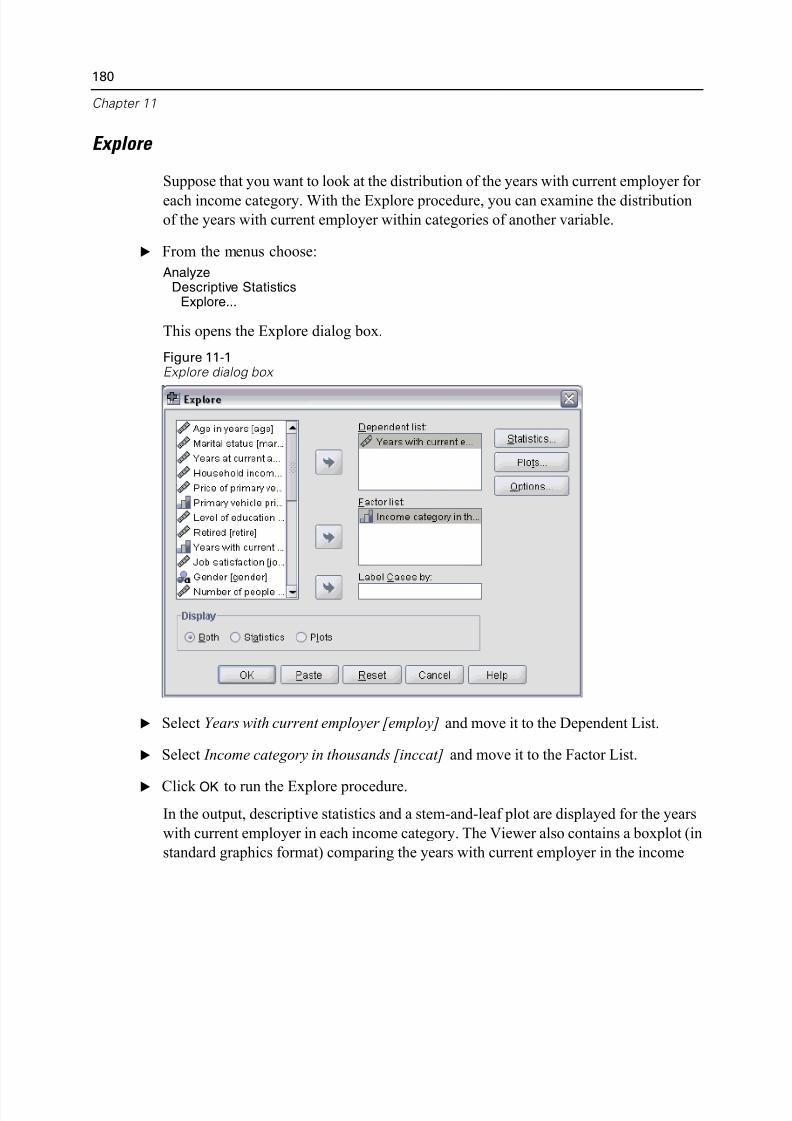
5/11/2018 SPSS Statistics Brief Guide 17.0 - slidepdf.com
http://slidepdf.com/reader/full/spss-statistics-brief-guide-170-55a2339b08a28 194/224
180
Chapter 11
Explore
Suppose that you want to look at the distribution of the years with current employer
each income category. With the Explore procedure, you can examine the distributioof the years with current employer within categories of another variable.
E From the menus choose:
AnalyzeDescriptive Statistics
Explore...
This opens the Explore dialog box.
Figure 11-1Explore dialog box
E Select Years with current employer [employ] and move it to the Dependent List.
E Select Income category in thousands [inccat] and move it to the Factor List.
E Click OK to run the Explore procedure.
In the output, descriptive statistics and a stem-and-leaf plot are displayed for the yea
with current employer in each income category. The Viewer also contains a boxplot
standard graphics format) comparing the years with current employer in the income
5/11/2018 SPSS Statistics Brief Guide 17.0 - slidepdf.com
http://slidepdf.com/reader/full/spss-statistics-brief-guide-170-55a2339b08a28 195/224
Additional Statistical Procedu
categories. For each category, the boxplot shows the median, interquartile range (25
to 75th percentile), outliers (indicated by O), and extreme values (indicated by *).
More about Summarizing Data
There are many ways to summarize data. For example, to calculate medians or
percentiles, use the Frequencies procedure or the Explore procedure. Here are som
additional methods:
Descriptives. For income, you can calculate standard scores, sometimes called z
scores. Use the Descriptives procedure and select Save standardized values as
variables.
Crosstabs. You can use the Crosstabs procedure to display the relationship betw
two or more categorical variables.
Summarize procedure. You can use the Summarize procedure to write to your
output window a listing of the actual values of age, gender, and income of the
first 25 or 50 cases.
E To run the Summarize procedure, from the menus choose:
AnalyzeReports
Case Summaries...
Comparing Means
The Compare Means submenu on the Analyze menu provides techniques for
displaying descriptive statistics and testing whether differences are significant betw
two means for both independent and paired samples. You can also use the One-Wa
ANOVA procedure to test whether differences are significant among more than two
independent means.
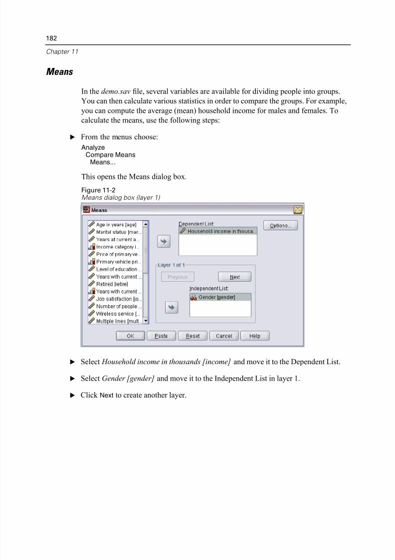
5/11/2018 SPSS Statistics Brief Guide 17.0 - slidepdf.com
http://slidepdf.com/reader/full/spss-statistics-brief-guide-170-55a2339b08a28 196/224
182
Chapter 11
Means
In the demo.sav file, several variables are available for dividing people into groups.
You can then calculate various statistics in order to compare the groups. For examp
you can compute the average (mean) household income for males and females. To
calculate the means, use the following steps:
E From the menus choose:
AnalyzeCompare Means
Means...
This opens the Means dialog box.
Figure 11-2
Means dialog box (layer 1)
E Select Household income in thousands [income] and move it to the Dependent List.
E Select Gender [gender] and move it to the Independent List in layer 1.
E Click Next to create another layer.
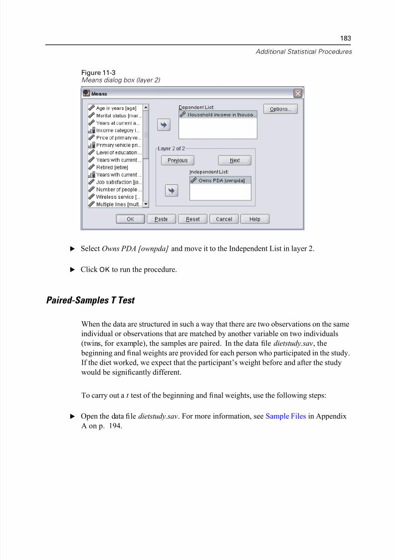
5/11/2018 SPSS Statistics Brief Guide 17.0 - slidepdf.com
http://slidepdf.com/reader/full/spss-statistics-brief-guide-170-55a2339b08a28 197/224
Additional Statistical Procedu
Figure 11-3Means dialog box (layer 2)
E Select Owns PDA [ownpda] and move it to the Independent List in layer 2.
E Click OK to run the procedure.
Paired-Samples T Test
When the data are structured in such a way that there are two observations on the sa
individual or observations that are matched by another variable on two individuals
(twins, for example), the samples are paired. In the data file dietstudy.sav, the
beginning and final weights are provided for each person who participated in the stu
If the diet worked, we expect that the participant’s weight before and after the study
would be significantly different.
To carry out a t test of the beginning and final weights, use the following steps:
E Open the data file dietstudy.sav. For more information, see Sample Files in Append
A on p. 194.
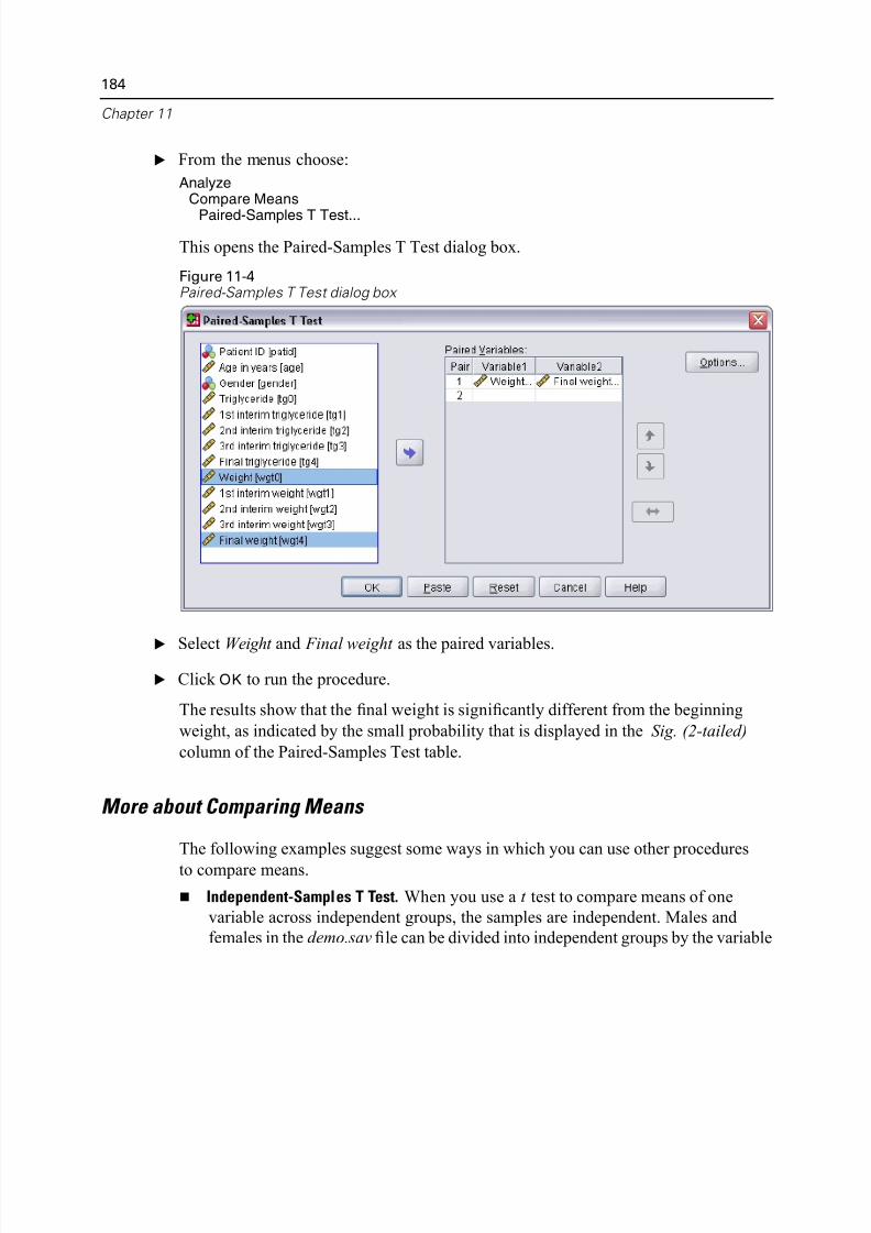
5/11/2018 SPSS Statistics Brief Guide 17.0 - slidepdf.com
http://slidepdf.com/reader/full/spss-statistics-brief-guide-170-55a2339b08a28 198/224
184
Chapter 11
E From the menus choose:
AnalyzeCompare Means
Paired-Samples T Test...
This opens the Paired-Samples T Test dialog box.
Figure 11-4Paired-Samples T Test dialog box
E Select Weight and Final weight as the paired variables.
E Click OK to run the procedure.
The results show that the final weight is significantly different from the beginning
weight, as indicated by the small probability that is displayed in the Sig. (2-tailed)
column of the Paired-Samples Test table.
More about Comparing Means
The following examples suggest some ways in which you can use other procedures
to compare means.
Independent-Samples T Test. When you use a t test to compare means of one
variable across independent groups, the samples are independent. Males and
females in the demo.sav file can be divided into independent groups by the varia
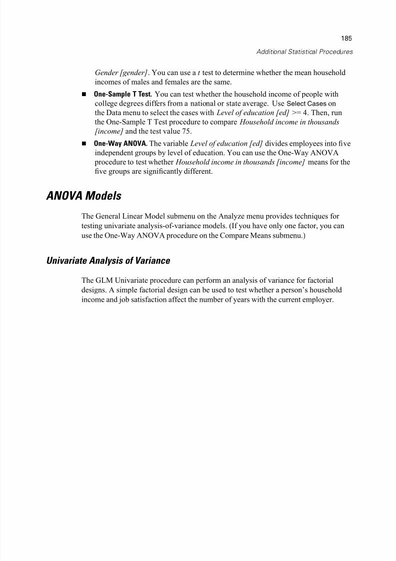
5/11/2018 SPSS Statistics Brief Guide 17.0 - slidepdf.com
http://slidepdf.com/reader/full/spss-statistics-brief-guide-170-55a2339b08a28 199/224
Additional Statistical Procedu
Gender [gender]. You can use a t test to determine whether the mean househol
incomes of males and females are the same.
One-Sample T Test. You can test whether the household income of people withcollege degrees differs from a national or state average. Use Select Cases on
the Data menu to select the cases with Level of education [ed] >= 4. Then, run
the One-Sample T Test procedure to compare Household income in thousands
[income] and the test value 75.
One-Way ANOVA. The variable Level of education [ed] divides employees into fi
independent groups by level of education. You can use the One-Way ANOVA
procedure to test whether Household income in thousands [income] means for
five groups are significantly different.
ANOVA Models The General Linear Model submenu on the Analyze menu provides techniques for
testing univariate analysis-of-variance models. (If you have only one factor, you ca
use the One-Way ANOVA procedure on the Compare Means submenu.)
Univariate Analysis of Variance
The GLM Univariate procedure can perform an analysis of variance for factorial
designs. A simple factorial design can be used to test whether a person’s householdincome and job satisfaction affect the number of years with the current employer.
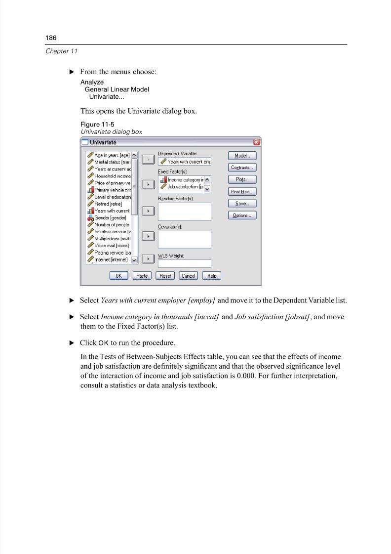
5/11/2018 SPSS Statistics Brief Guide 17.0 - slidepdf.com
http://slidepdf.com/reader/full/spss-statistics-brief-guide-170-55a2339b08a28 200/224
186
Chapter 11
E From the menus choose:
AnalyzeGeneral Linear Model
Univariate...
This opens the Univariate dialog box.
Figure 11-5Univariate dialog box
E Select Years with current employer [employ] and move it to the Dependent Variable
E Select Income category in thousands [inccat] and Job satisfaction [jobsat], and mo
them to the Fixed Factor(s) list.
E Click OK to run the procedure.
In the Tests of Between-Subjects Effects table, you can see that the effects of incom
and job satisfaction are definitely significant and that the observed significance leve
of the interaction of income and job satisfaction is 0.000. For further interpretation
consult a statistics or data analysis textbook.
5/11/2018 SPSS Statistics Brief Guide 17.0 - slidepdf.com
http://slidepdf.com/reader/full/spss-statistics-brief-guide-170-55a2339b08a28 201/224
Additional Statistical Procedu
Correlating Variables
The Correlate submenu on the Analyze menu provides measures of association for t
or more numeric variables. The examples in this topic use the data file Employee
data.sav.
Bivariate Correlations
The Bivariate Correlations procedure computes statistics such as Pearson’s correlati
coef ficient. Correlations measure how variables or rank orders are related. Correlati
coef ficients range in value from –1 (a perfect negative relationship) and +1 (a perfe
positive relationship). A value of 0 indicates no linear relationship.
For example, you can use Pearson’s correlation coef ficient to see if there is a strolinear association between Current Salary [salary] and Beginning Salary [salbegin]
the data file Employee data.sav.
Partial Correlations
The Partial Correlations procedure calculates partial correlation coef ficients that
describe the relationship between two variables while adjusting for the effects of on
or more additional variables.
You can estimate the correlation between Current Salary [salary] and Beginning
Salary [salbegin], controlling for the linear effects of Months since Hire [jobtime]
and Previous Experience [prevexp]. The number of control variables determines th
order of the partial correlation coef ficient.
To carry out this Partial Correlations procedure, use the following steps:
E Open the Employee data.sav file, which is usually in the installation directory.
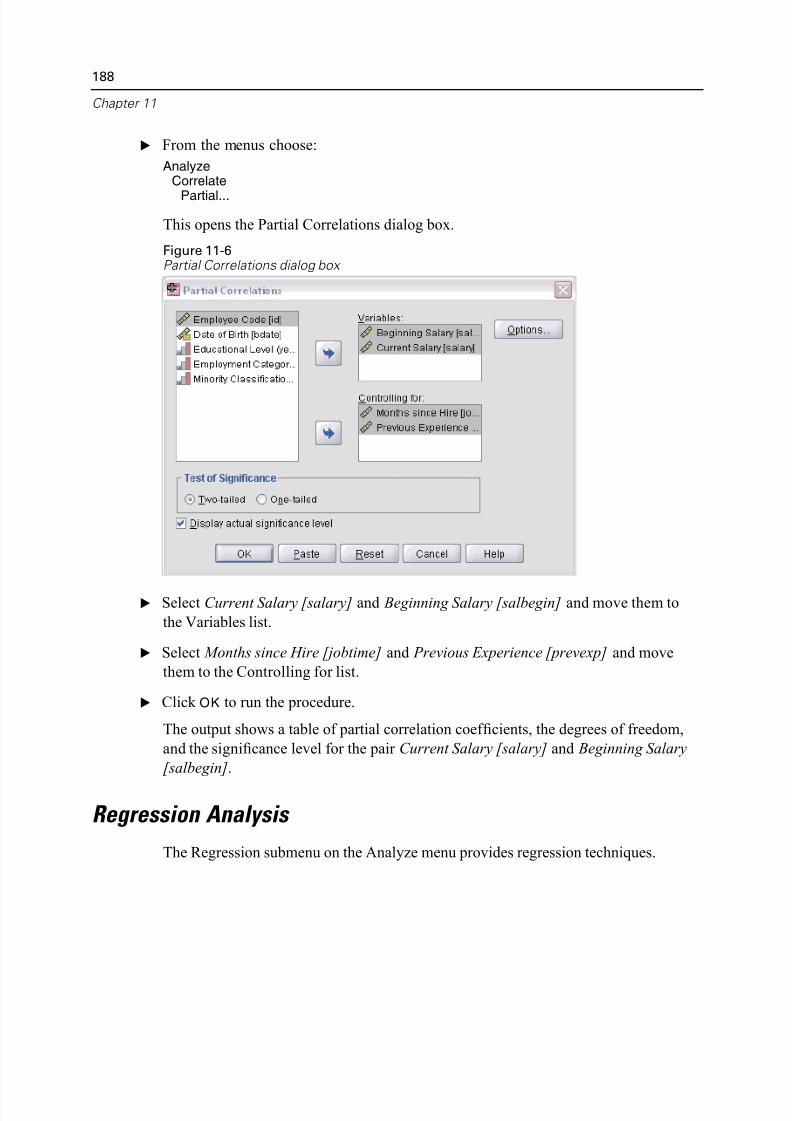
5/11/2018 SPSS Statistics Brief Guide 17.0 - slidepdf.com
http://slidepdf.com/reader/full/spss-statistics-brief-guide-170-55a2339b08a28 202/224
188
Chapter 11
E From the menus choose:
AnalyzeCorrelate
Partial...
This opens the Partial Correlations dialog box.
Figure 11-6Partial Correlations dialog box
E Select Current Salary [salary] and Beginning Salary [salbegin] and move them to
the Variables list.
E Select Months since Hire [jobtime] and Previous Experience [prevexp] and move
them to the Controlling for list.
E Click OK to run the procedure.
The output shows a table of partial correlation coef ficients, the degrees of freedom,
and the significance level for the pair Current Salary [salary] and Beginning Salary
[salbegin].
Regression Analysis
The Regression submenu on the Analyze menu provides regression techniques.
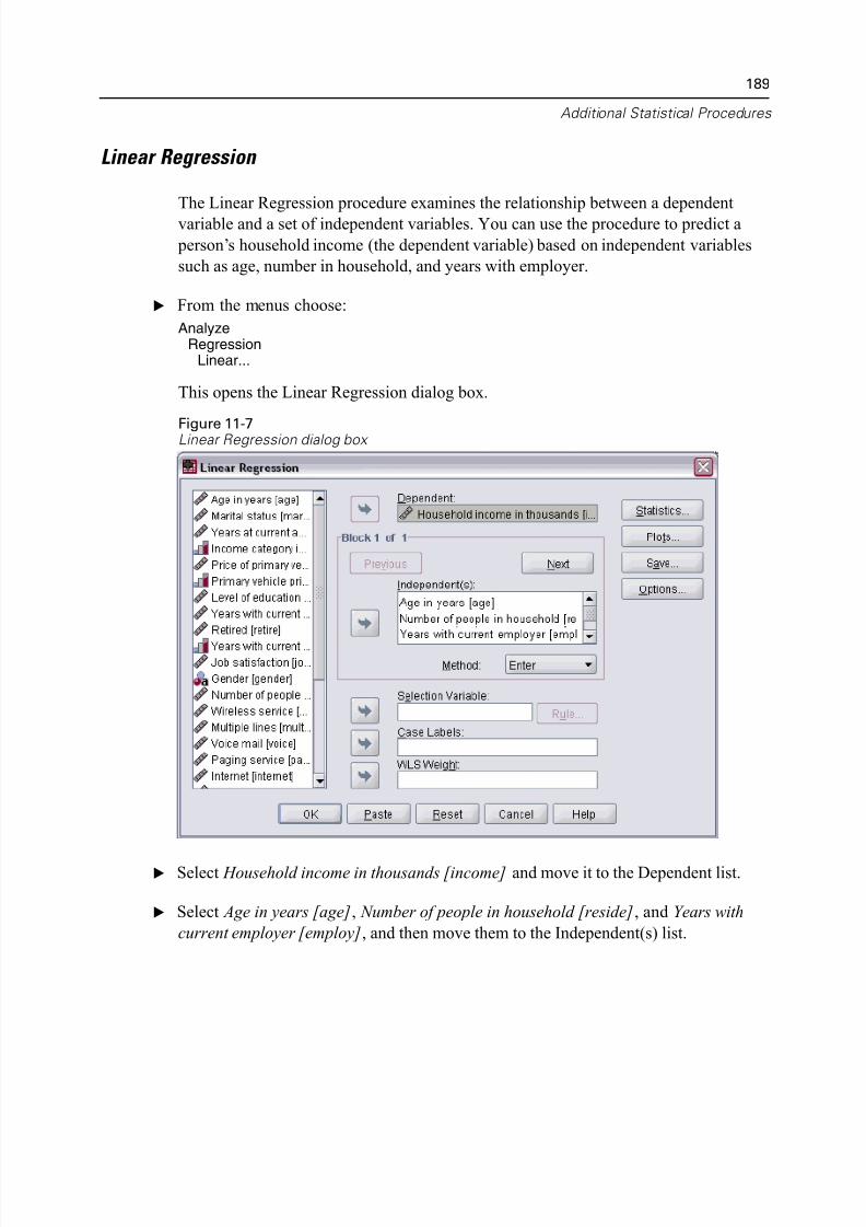
5/11/2018 SPSS Statistics Brief Guide 17.0 - slidepdf.com
http://slidepdf.com/reader/full/spss-statistics-brief-guide-170-55a2339b08a28 203/224
Additional Statistical Procedu
Linear Regression
The Linear Regression procedure examines the relationship between a dependent
variable and a set of independent variables. You can use the procedure to predict a
person’s household income (the dependent variable) based on independent variable
such as age, number in household, and years with employer.
E From the menus choose:
AnalyzeRegression
Linear...
This opens the Linear Regression dialog box.
Figure 11-7Linear Regression dialog box
E Select Household income in thousands [income] and move it to the Dependent list.
E Select Age in years [age], Number of people in household [reside], and Years with
current employer [employ], and then move them to the Independent(s) list.
5/11/2018 SPSS Statistics Brief Guide 17.0 - slidepdf.com
http://slidepdf.com/reader/full/spss-statistics-brief-guide-170-55a2339b08a28 204/224
190
Chapter 11
E Click OK to run the procedure.
The output contains goodness-of-fit statistics and the partial regression coef ficients
the variables.
Examining Fit. To see how well the regression model fits your data, you can examin
the residuals and other types of diagnostics that this procedure provides. In the Line
Regression dialog box, click Save to see a list of the new variables that you can add
your data file. If you generate any of these variables, they will not be available in a
later session unless you save the data file.
Methods. If you have collected a large number of independent variables and want to
build a regression model that includes only variables that are statistically related to
dependent variable, you can choose a method from the drop-down list. For example
you select Stepwise in the above example, only variables that meet the criteria in thLinear Regression Options dialog box are entered in the equation.
Nonparametric Tests
The Nonparametric Tests submenu on the Analyze menu provides nonparametric te
for one sample or for two or more paired or independent samples. Nonparametric
tests do not require assumptions about the shape of the distributions from which the
data originate.
Chi-Square
The Chi-Square Test procedure is used to test hypotheses about the relative proport
of cases falling into several mutually exclusive groups. You can test the hypothesis
that people who participated in the survey occur in the same proportions of gender
the general population (50% males, 50% females).
In this example, you will need to recode the string variable Gender [gender] into
a numeric variable before you can run the procedure.
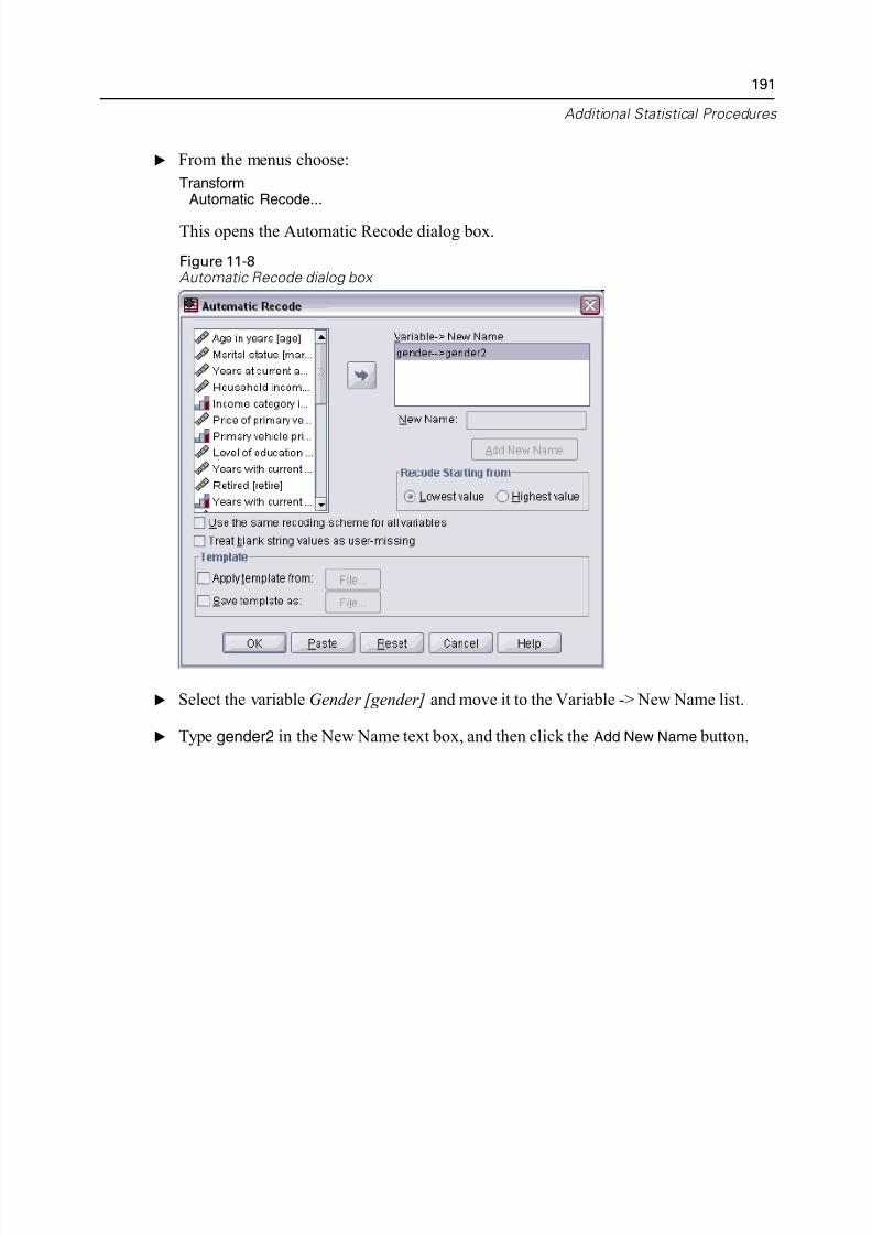
5/11/2018 SPSS Statistics Brief Guide 17.0 - slidepdf.com
http://slidepdf.com/reader/full/spss-statistics-brief-guide-170-55a2339b08a28 205/224
Additional Statistical Procedu
E From the menus choose:
TransformAutomatic Recode...
This opens the Automatic Recode dialog box.
Figure 11-8Automatic Recode dialog box
E Select the variable Gender [gender] and move it to the Variable -> New Name list.
E Type gender2 in the New Name text box, and then click the Add New Name button.
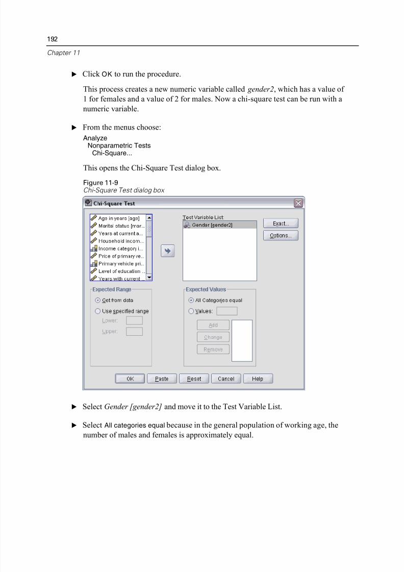
5/11/2018 SPSS Statistics Brief Guide 17.0 - slidepdf.com
http://slidepdf.com/reader/full/spss-statistics-brief-guide-170-55a2339b08a28 206/224
192
Chapter 11
E Click OK to run the procedure.
This process creates a new numeric variable called gender2, which has a value of
1 for females and a value of 2 for males. Now a chi-square test can be run with anumeric variable.
E From the menus choose:
AnalyzeNonparametric Tests
Chi-Square...
This opens the Chi-Square Test dialog box.
Figure 11-9Chi-Square Test dialog box
E Select Gender [gender2] and move it to the Test Variable List.
E Select All categories equal because in the general population of working age, the
number of males and females is approximately equal.

5/11/2018 SPSS Statistics Brief Guide 17.0 - slidepdf.com
http://slidepdf.com/reader/full/spss-statistics-brief-guide-170-55a2339b08a28 207/224
Additional Statistical Procedu
E Click OK to run the procedure.
The output shows a table of the expected and residual values for the categories. Th
significance of the chi-square test is 0.6. For more information about interpretation the statistics, consult a statistics or data analysis textbook.
5/11/2018 SPSS Statistics Brief Guide 17.0 - slidepdf.com
http://slidepdf.com/reader/full/spss-statistics-brief-guide-170-55a2339b08a28 208/224
Append
A
Sample Files
The sample files installed with the product can be found in the Samples subdirectory
the installation directory. There is a separate folder within the Samples subdirectory
each of the following languages: English, French, German, Italian, Japanese, Korea
Polish, Russian, Simplified Chinese, Spanish, and Traditional Chinese.
Not all sample files are available in all languages. If a sample file is not available in
language, that language folder contains an English version of the sample file.
Descriptions
Following are brief descriptions of the sample files used in various examples
throughout the documentation.
accidents.sav. This is a hypothetical data file that concerns an insurance compan
that is studying age and gender risk factors for automobile accidents in a given
region. Each case corresponds to a cross-classification of age category and gend
adl.sav. This is a hypothetical data file that concerns efforts to determine the
benefits of a proposed type of therapy for stroke patients. Physicians randomly
assigned female stroke patients to one of two groups. The first received the
standard physical therapy, and the second received an additional emotional
therapy. Three months following the treatments, each patient’s abilities to perfo
common activities of daily life were scored as ordinal variables.
advert.sav. This is a hypothetical data file that concerns a retailer’s efforts to
examine the relationship between money spent on advertising and the resulting
sales. To this end, they have collected past sales figures and the associated
advertising costs..
194
5/11/2018 SPSS Statistics Brief Guide 17.0 - slidepdf.com
http://slidepdf.com/reader/full/spss-statistics-brief-guide-170-55a2339b08a28 209/224
Sample F
aflatoxin.sav. This is a hypothetical data file that concerns the testing of corn cro
for aflatoxin, a poison whose concentration varies widely between and within c
yields. A grain processor has received 16 samples from each of 8 crop yields an
measured the alfatoxin levels in parts per billion (PPB).
aflatoxin20.sav. This data file contains the aflatoxin measurements from each of
16 samples from yields 4 and 8 from the a fl atoxin.sav data file.
anorectic.sav. While working toward a standardized symptomatology of
anorectic/bulimic behavior, researchers made a study of 55 adolescents with
known eating disorders. Each patient was seen four times over four years, for a
total of 220 observations. At each observation, the patients were scored for each
16 symptoms. Symptom scores are missing for patient 71 at time 2, patient 76
time 2, and patient 47 at time 3, leaving 217 valid observations.
autoaccidents.sav. This is a hypothetical datafi
le that concerns the efforts of aninsurance analyst to model the number of automobile accidents per driver whil
also accounting for driver age and gender. Each case represents a separate driv
and records the driver’s gender, age in years, and number of automobile acciden
in the last five years.
band.sav. This data file contains hypothetical weekly sales figures of music CD
for a band. Data for three possible predictor variables are also included.
bankloan.sav. This is a hypothetical data file that concerns a bank’s efforts to red
the rate of loan defaults. The file contains financial and demographic informati
on 850 past and prospective customers. The first 700 cases are customers who
were previously given loans. The last 150 cases are prospective customers thatthe bank needs to classify as good or bad credit risks.
bankloan_binning.sav. This is a hypothetical data file containing financial and
demographic information on 5,000 past customers.
behavior.sav. In a classic example , 52 students were asked to rate the combinati
of 15 situations and 15 behaviors on a 10-point scale ranging from 0=“extreme
appropriate” to 9=“extremely inappropriate.” Averaged over individuals, the
values are taken as dissimilarities.
behavior_ini.sav. This data file contains an initial configuration for a
two-dimensional solution for behavior.sav.
brakes.sav. This is a hypothetical data file that concerns quality control at a fact
that produces disc brakes for high-performance automobiles. The data file conta
diameter measurements of 16 discs from each of 8 production machines. The
target diameter for the brakes is 322 millimeters.
5/11/2018 SPSS Statistics Brief Guide 17.0 - slidepdf.com
http://slidepdf.com/reader/full/spss-statistics-brief-guide-170-55a2339b08a28 210/224
196
Appendix A
breakfast.sav. In a classic study , 21 Wharton School MBA students and their
spouses were asked to rank 15 breakfast items in order of preference with 1=“m
preferred” to 15=“least preferred.” Their preferences were recorded under six
different scenarios, from “Overall preference” to “Snack, with beverage only.”
breakfast-overall.sav. This data file contains the breakfast item preferences for t
first scenario, “Overall preference,” only.
broadband_1.sav. This is a hypothetical data file containing the number of
subscribers, by region, to a national broadband service. The data file contains
monthly subscriber numbers for 85 regions over a four-year period.
broadband_2.sav. This data file is identical to broadband_1.sav but contains dat
for three additional months.
car_insurance_claims.sav. A dataset presented and analyzed elsewhere concern
damage claims for cars. The average claim amount can be modeled as havinga gamma distribution, using an inverse link function to relate the mean of the
dependent variable to a linear combination of the policyholder age, vehicle typ
and vehicle age. The number of claims filed can be used as a scaling weight.
car_sales.sav. This data file contains hypothetical sales estimates, list prices,
and physical specifications for various makes and models of vehicles. The list
prices and physical specifications were obtained alternately from edmunds.com
and manufacturer sites.
carpet.sav. In a popular example , a company interested in marketing a new
carpet cleaner wants to examine the influence of five factors on consumer
preference—package design, brand name, price, a Good Housekeeping seal, ana money-back guarantee. There are three factor levels for package design, each
one differing in the location of the applicator brush; three brand names (K2R,
Glory, and Bissell); three price levels; and two levels (either no or yes) for each
of the last two factors. Ten consumers rank 22 profiles defined by these factors
The variable Preference contains the rank of the average rankings for each profi
Low rankings correspond to high preference. This variable reflects an overall
measure of preference for each profile.
carpet_prefs.sav. This data file is based on the same example as described for
carpet.sav, but it contains the actual rankings collected from each of the 10
consumers. The consumers were asked to rank the 22 product profiles from themost to the least preferred. The variables PREF1 through PREF22 contain the
identifiers of the associated profiles, as defined in carpet_plan.sav.
5/11/2018 SPSS Statistics Brief Guide 17.0 - slidepdf.com
http://slidepdf.com/reader/full/spss-statistics-brief-guide-170-55a2339b08a28 211/224
Sample F
catalog.sav. This data file contains hypothetical monthly sales figures for three
products sold by a catalog company. Data for five possible predictor variables
are also included.
catalog_seasfac.sav. This data file is the same as catalog.sav except for the
addition of a set of seasonal factors calculated from the Seasonal Decompositio
procedure along with the accompanying date variables.
cellular.sav. This is a hypothetical data file that concerns a cellular phone
company’s efforts to reduce churn. Churn propensity scores are applied to
accounts, ranging from 0 to 100. Accounts scoring 50 or above may be looking
change providers.
ceramics.sav. This is a hypothetical data file that concerns a manufacturer’s effo
to determine whether a new premium alloy has a greater heat resistance than a
standard alloy. Each case represents a separate test of one of the alloys; the heawhich the bearing failed is recorded.
cereal.sav. This is a hypothetical data file that concerns a poll of 880 people abo
their breakfast preferences, also noting their age, gender, marital status, and
whether or not they have an active lifestyle (based on whether they exercise at
least twice a week). Each case represents a separate respondent.
clothing_defects.sav. This is a hypothetical data file that concerns the quality
control process at a clothing factory. From each lot produced at the factory, the
inspectors take a sample of clothes and count the number of clothes that are
unacceptable.
coffee.sav. This data file pertains to perceived images of six iced-coffee brands For each of 23 iced-coffee image attributes, people selected all brands that wer
described by the attribute. The six brands are denoted AA, BB, CC, DD, EE, an
FF to preserve confidentiality.
contacts.sav. This is a hypothetical data file that concerns the contact lists for a
group of corporate computer sales representatives. Each contact is categorized
by the department of the company in which they work and their company ranks
Also recorded are the amount of the last sale made, the time since the last sale,
and the size of the contact’s company.
creditpromo.sav. This is a hypothetical data file that concerns a department store
efforts to evaluate the effectiveness of a recent credit card promotion. To thisend, 500 cardholders were randomly selected. Half received an ad promoting a
reduced interest rate on purchases made over the next three months. Half receiv
a standard seasonal ad.
5/11/2018 SPSS Statistics Brief Guide 17.0 - slidepdf.com
http://slidepdf.com/reader/full/spss-statistics-brief-guide-170-55a2339b08a28 212/224
198
Appendix A
customer_dbase.sav. This is a hypothetical data file that concerns a company’s
efforts to use the information in its data warehouse to make special offers to
customers who are most likely to reply. A subset of the customer base was selec
at random and given the special offers, and their responses were recorded.
customer_information.sav. A hypothetical data file containing customer mailing
information, such as name and address.
customers_model.sav. This file contains hypothetical data on individuals targete
by a marketing campaign. These data include demographic information, a
summary of purchasing history, and whether or not each individual responded t
the campaign. Each case represents a separate individual.
customers_new.sav. This file contains hypothetical data on individuals who are
potential candidates for a marketing campaign. These data include demographi
information and a summary of purchasing history for each individual. Each casrepresents a separate individual.
debate.sav. This is a hypothetical data file that concerns paired responses to a
survey from attendees of a political debate before and after the debate. Each ca
corresponds to a separate respondent.
debate_aggregate.sav. This is a hypothetical data file that aggregates the respon
in debate.sav. Each case corresponds to a cross-classification of preference bef
and after the debate.
demo.sav. This is a hypothetical data file that concerns a purchased customer
database, for the purpose of mailing monthly offers. Whether or not the custom
responded to the offer is recorded, along with various demographic information
demo_cs_1.sav. This is a hypothetical data file that concerns the first step of
a company’s efforts to compile a database of survey information. Each case
corresponds to a different city, and the region, province, district, and city
identification are recorded.
demo_cs_2.sav. This is a hypothetical data file that concerns the second step
of a company’s efforts to compile a database of survey information. Each case
corresponds to a different household unit from cities selected in the first step, a
the region, province, district, city, subdivision, and unit identification are record
The sampling information from the first two stages of the design is also include
demo_cs.sav. This is a hypothetical data file that contains survey information
collected using a complex sampling design. Each case corresponds to a differen
household unit, and various demographic and sampling information is recorded
5/11/2018 SPSS Statistics Brief Guide 17.0 - slidepdf.com
http://slidepdf.com/reader/full/spss-statistics-brief-guide-170-55a2339b08a28 213/224
Sample F
dietstudy.sav. This hypothetical data file contains the results of a study of the
“Stillman diet” . Each case corresponds to a separate subject and records his or
pre- and post-diet weights in pounds and triglyceride levels in mg/100 ml.
dischargedata.sav. This is a data file concerning Seasonal Patterns of Winnipeg
Hospital Use, from the Manitoba Centre for Health Policy.
dvdplayer.sav. This is a hypothetical data file that concerns the development of
new DVD player. Using a prototype, the marketing team has collected focus
group data. Each case corresponds to a separate surveyed user and records som
demographic information about them and their responses to questions about the
prototype.
flying.sav. This data file contains the flying mileages between 10 American citie
german_credit.sav. This data file is taken from the “German credit” dataset in th
Repository of Machine Learning Databases at the University of California, Irvin grocery_1month.sav. This hypothetical data file is the grocery_coupons.sav data
with the weekly purchases “rolled-up” so that each case corresponds to a separa
customer. Some of the variables that changed weekly disappear as a result, and
the amount spent recorded is now the sum of the amounts spent during the four
weeks of the study.
grocery_coupons.sav. This is a hypothetical data file that contains survey data
collected by a grocery store chain interested in the purchasing habits of their
customers. Each customer is followed for four weeks, and each case correspon
to a separate customer-week and records information about where and how the
customer shops, including how much was spent on groceries during that week.
guttman.sav. Bell presented a table to illustrate possible social groups. Guttman
used a portion of this table, in which five variables describing such things as soc
interaction, feelings of belonging to a group, physical proximity of members,
and formality of the relationship were crossed with seven theoretical social
groups, including crowds (for example, people at a football game), audiences
(for example, people at a theater or classroom lecture), public (for example,
newspaper or television audiences), mobs (like a crowd but with much more
intense interaction), primary groups (intimate), secondary groups (voluntary),
and the modern community (loose confederation resulting from close physical
proximity and a need for specialized services). healthplans.sav. This is a hypothetical data file that concerns an insurance group
efforts to evaluate four different health care plans for small employers. Twelve
employers are recruited to rank the plans by how much they would prefer to
5/11/2018 SPSS Statistics Brief Guide 17.0 - slidepdf.com
http://slidepdf.com/reader/full/spss-statistics-brief-guide-170-55a2339b08a28 214/224
200
Appendix A
offer them to their employees. Each case corresponds to a separate employer
and records the reactions to each plan.
health_funding.sav. This is a hypothetical datafi
le that contains data on health cfunding (amount per 100 population), disease rates (rate per 10,000 population
and visits to health care providers (rate per 10,000 population). Each case
represents a different city.
hivassay.sav. This is a hypothetical data file that concerns the efforts of a
pharmaceutical lab to develop a rapid assay for detecting HIV infection. The
results of the assay are eight deepening shades of red, with deeper shades indicat
greater likelihood of infection. A laboratory trial was conducted on 2,000 bloo
samples, half of which were infected with HIV and half of which were clean.
hourlywagedata.sav. This is a hypothetical data file that concerns the hourly wag
of nurses from of fi
ce and hospital positions and with varying levels of experien insure.sav. This is a hypothetical data file that concerns an insurance company t
is studying the risk factors that indicate whether a client will have to make a cla
on a 10-year term life insurance contract. Each case in the data file represents a
pair of contracts, one of which recorded a claim and the other didn’t, matched
on age and gender.
judges.sav. This is a hypothetical data file that concerns the scores given by train
judges (plus one enthusiast) to 300 gymnastics performances. Each row represe
a separate performance; the judges viewed the same performances.
kinship_dat.sav. Rosenberg and Kim set out to analyze 15 kinship terms (aunt,
brother, cousin, daughter, father, granddaughter, grandfather, grandmother,grandson, mother, nephew, niece, sister, son, uncle). They asked four groups
of college students (two female, two male) to sort these terms on the basis of
similarities. Two groups (one female, one male) were asked to sort twice, with
second sorting based on a different criterion from the first sort. Thus, a total of
“sources” were obtained. Each source corresponds to a proximity matr
whose cells are equal to the number of people in a source minus the number of
times the objects were partitioned together in that source.
kinship_ini.sav. This data file contains an initial configuration for a
three-dimensional solution for kinship_dat.sav.
kinship_var.sav. This data file contains independent variables gender , gener (atioand degree (of separation) that can be used to interpret the dimensions of a solut
for kinship_dat.sav. Specifically, they can be used to restrict the space of the
solution to a linear combination of these variables.
5/11/2018 SPSS Statistics Brief Guide 17.0 - slidepdf.com
http://slidepdf.com/reader/full/spss-statistics-brief-guide-170-55a2339b08a28 215/224
Sample F
mailresponse.sav. This is a hypothetical data file that concerns the efforts of a
clothing manufacturer to determine whether using first class postage for direct
mailings results in faster responses than bulk mail. Order-takers record how ma
weeks after the mailing each order is taken.
marketvalues.sav. This data file concerns home sales in a new housing developm
in Algonquin, Ill., during the years from 1999–2000. These sales are a matter
of public record.
mutualfund.sav. This data file concerns stock market information for various tec
stocks listed on the S&P 500. Each case corresponds to a separate company.
nhis2000_subset.sav. The National Health Interview Survey (NHIS) is a large,
population-based survey of the U.S. civilian population. Interviews are
carried out face-to-face in a nationally representative sample of households.
Demographic information and observations about health behaviors and statusare obtained for members of each household. This data file contains a subset
of information from the 2000 survey. National Center for Health Statistics.
National Health Interview Survey, 2000. Public-use data file and documentatio
ftp://ftp.cdc.gov/pub/Health_Statistics/NCHS/Datasets/NHIS/2000/ . Accessed
2003.
ozone.sav. The data include 330 observations on six meteorological variables fo
predicting ozone concentration from the remaining variables. Previous research
, , among others found nonlinearities among these variables, which hinder stand
regression approaches.
pain_medication.sav. This hypothetical datafi
le contains the results of a clinicatrial for anti-inflammatory medication for treating chronic arthritic pain. Of
particular interest is the time it takes for the drug to take effect and how it
compares to an existing medication.
patient_los.sav. This hypothetical data file contains the treatment records of
patients who were admitted to the hospital for suspected myocardial infarction
(MI, or “heart attack”). Each case corresponds to a separate patient and records
many variables related to their hospital stay.
patlos_sample.sav. This hypothetical data file contains the treatment records of
sample of patients who received thrombolytics during treatment for myocardia
infarction (MI, or “heart attack”). Each case corresponds to a separate patient arecords many variables related to their hospital stay.
5/11/2018 SPSS Statistics Brief Guide 17.0 - slidepdf.com
http://slidepdf.com/reader/full/spss-statistics-brief-guide-170-55a2339b08a28 216/224
202
Appendix A
polishing.sav. This is the “Nambeware Polishing Times” data file from the Data
Story Library. It concerns the efforts of a metal tableware manufacturer (Namb
Mills, Santa Fe, N. M.) to plan its production schedule. Each case represents a
different item in the product line. The diameter, polishing time, price, and produtype are recorded for each item.
poll_cs.sav. This is a hypothetical data file that concerns pollsters’ efforts to
determine the level of public support for a bill before the legislature. The cases
correspond to registered voters. Each case records the county, township, and
neighborhood in which the voter lives.
poll_cs_sample.sav. This hypothetical data file contains a sample of the voters
listed in poll_cs.sav. The sample was taken according to the design specified in
the poll.csplan plan file, and this data file records the inclusion probabilities an
sample weights. Note, however, that because the sampling plan makes use of
a probability-proportional-to-size (PPS) method, there is also a file containing
the joint selection probabilities ( poll_jointprob.sav). The additional variables
corresponding to voter demographics and their opinion on the proposed bill we
collected and added the data file after the sample as taken.
property_assess.sav. This is a hypothetical data file that concerns a county
assessor’s efforts to keep property value assessments up to date on limited
resources. The cases correspond to properties sold in the county in the past yea
Each case in the data file records the township in which the property lies, the
assessor who last visited the property, the time since that assessment, the valuat
made at that time, and the sale value of the property.
property_assess_cs.sav. This is a hypothetical data file that concerns a state
assessor’s efforts to keep property value assessments up to date on limited
resources. The cases correspond to properties in the state. Each case in the dat
file records the county, township, and neighborhood in which the property lies,
time since the last assessment, and the valuation made at that time.
property_assess_cs_sample.sav. This hypothetical data file contains a sample o
the properties listed in property_assess_cs.sav. The sample was taken accordin
to the design specified in the property_assess.csplan plan file, and this data file
records the inclusion probabilities and sample weights. The additional variable
Current value was collected and added to the data file after the sample was take
recidivism.sav. This is a hypothetical data file that concerns a government law
enforcement agency’s efforts to understand recidivism rates in their area of
jurisdiction. Each case corresponds to a previous offender and records their
5/11/2018 SPSS Statistics Brief Guide 17.0 - slidepdf.com
http://slidepdf.com/reader/full/spss-statistics-brief-guide-170-55a2339b08a28 217/224
Sample F
demographic information, some details of their first crime, and then the time un
their second arrest, if it occurred within two years of the first arrest.
recidivism_cs_sample.sav. This is a hypothetical datafi
le that concerns agovernment law enforcement agency’s efforts to understand recidivism rates
in their area of jurisdiction. Each case corresponds to a previous offender,
released from their first arrest during the month of June, 2003, and records
their demographic information, some details of their first crime, and the data
of their second arrest, if it occurred by the end of June, 2006. Offenders were
selected from sampled departments according to the sampling plan specified in
recidivism_cs.csplan; because it makes use of a probability-proportional-to-siz
(PPS) method, there is also a file containing the joint selection probabilities
(recidivism_cs_jointprob.sav ).
rfm_transactions.sav. A hypothetical data file containing purchase transaction
data, including date of purchase, item(s) purchased, and monetary amount of
each transaction.
salesperformance.sav. This is a hypothetical data file that concerns the evaluatio
of two new sales training courses. Sixty employees, divided into three groups, a
receive standard training. In addition, group 2 gets technical training; group 3,
a hands-on tutorial. Each employee was tested at the end of the training course
and their score recorded. Each case in the data file represents a separate trainee
and records the group to which they were assigned and the score they received
on the exam.
satisf.sav. This is a hypothetical data file that concerns a satisfaction survey
conducted by a retail company at 4 store locations. 582 customers were survey
in all, and each case represents the responses from a single customer.
screws.sav. This data file contains information on the characteristics of screws,
bolts, nuts, and tacks .
shampoo_ph.sav. This is a hypothetical data file that concerns the quality contro
a factory for hair products. At regular time intervals, six separate output batche
are measured and their pH recorded. The target range is 4.5–5.5.
ships.sav. A dataset presented and analyzed elsewhere that concerns damage to
cargo ships caused by waves. The incident counts can be modeled as occurring
at a Poisson rate given the ship type, construction period, and service period.The aggregate months of service for each cell of the table formed by the
cross-classification of factors provides values for the exposure to risk.
5/11/2018 SPSS Statistics Brief Guide 17.0 - slidepdf.com
http://slidepdf.com/reader/full/spss-statistics-brief-guide-170-55a2339b08a28 218/224
204
Appendix A
site.sav. This is a hypothetical data file that concerns a company’s efforts to cho
new sites for their expanding business. They have hired two consultants to
separately evaluate the sites, who, in addition to an extended report, summarize
each site as a “good,” “fair,” or “poor” prospect.
siteratings.sav. This is a hypothetical data file that concerns the beta testing of a
e-commerce firm’s new Web site. Each case represents a separate beta tester, w
scored the usability of the site on a scale from 0–20.
smokers.sav. This data file is abstracted from the 1998 National Household Surv
of Drug Abuse and is a probability sample of American households. Thus, the
first step in an analysis of this data file should be to weight the data to reflect
population trends.
smoking.sav. This is a hypothetical table introduced by Greenacre . The table o
interest is formed by the crosstabulation of smoking behavior by job category. Tvariable Staff Group contains the job categories Sr Managers, Jr Managers, Sr
Employees, Jr Employees, and Secretaries, plus the category National Average
which can be used as supplementary to an analysis. The variable Smoking conta
the behaviors None, Light , Medium, and Heavy, plus the categories No Alcohol
and Alcohol, which can be used as supplementary to an analysis.
storebrand.sav. This is a hypothetical data file that concerns a grocery store
manager’s efforts to increase sales of the store brand detergent relative to other
brands. She puts together an in-store promotion and talks with customers at
check-out. Each case represents a separate customer.
stores.sav. This datafi
le contains hypothetical monthly market share data for two competing grocery stores. Each case represents the market share data for a
given month.
stroke_clean.sav. This hypothetical data file contains the state of a medical
database after it has been cleaned using procedures in the Data Preparation opti
stroke_invalid.sav. This hypothetical data file contains the initial state of a medi
database and contains several data entry errors.
stroke_survival. This hypothetical data file concerns survival times for patients
exiting a rehabilitation program post-ischemic stroke face a number of challeng
Post-stroke, the occurrence of myocardial infarction, ischemic stroke, or
hemorrhagic stroke is noted and the time of the event recorded. The sample isleft-truncated because it only includes patients who survived through the end o
the rehabilitation program administered post-stroke.
5/11/2018 SPSS Statistics Brief Guide 17.0 - slidepdf.com
http://slidepdf.com/reader/full/spss-statistics-brief-guide-170-55a2339b08a28 219/224
Sample F
stroke_valid.sav. This hypothetical data file contains the state of a medical datab
after the values have been checked using the Validate Data procedure. It still
contains potentially anomalous cases.
survey_sample.sav. This hypothetical data file contains survey data, including
demographic data and various attitude measures.
tastetest.sav. This is a hypothetical data file that concerns the effect of mulch co
on the taste of crops. Strawberries grown in red, blue, and black mulch were rat
by taste-testers on an ordinal scale of 1 to 5 (far below to far above average). E
case represents a separate taste-tester.
telco.sav. This is a hypothetical data file that concerns a telecommunications
company’s efforts to reduce churn in their customer base. Each case correspond
to a separate customer and records various demographic and service usage
information. telco_extra.sav. This data file is similar to the telco.sav data file, but the “tenure
and log-transformed customer spending variables have been removed and repla
by standardized log-transformed customer spending variables.
telco_missing.sav. This data file is a subset of the telco.sav data file, but some o
the demographic data values have been replaced with missing values.
testmarket.sav. This hypothetical data file concerns a fast food chain’s plans to
add a new item to its menu. There are three possible campaigns for promoting
the new product, so the new item is introduced at locations in several randomly
selected markets. A different promotion is used at each location, and the weekl
sales of the new item are recorded for the first four weeks. Each case corresponto a separate location-week.
testmarket_1month.sav. This hypothetical data file is the testmarket.sav data file
with the weekly sales “rolled-up” so that each case corresponds to a separate
location. Some of the variables that changed weekly disappear as a result, and t
sales recorded is now the sum of the sales during the four weeks of the study.
tree_car.sav. This is a hypothetical data file containing demographic and vehicl
purchase price data.
tree_credit.sav. This is a hypothetical data file containing demographic and ban
loan history data.
tree_missing_data.sav This is a hypothetical data file containing demographic an
bank loan history data with a large number of missing values.
5/11/2018 SPSS Statistics Brief Guide 17.0 - slidepdf.com
http://slidepdf.com/reader/full/spss-statistics-brief-guide-170-55a2339b08a28 220/224
206
Appendix A
tree_score_car.sav. This is a hypothetical data file containing demographic and
vehicle purchase price data.
tree_textdata.sav. A simple datafi
le with only two variables intended primarilyto show the default state of variables prior to assignment of measurement level
and value labels.
tv-survey.sav. This is a hypothetical data file that concerns a survey conducted b
TV studio that is considering whether to extend the run of a successful program
906 respondents were asked whether they would watch the program under vario
conditions. Each row represents a separate respondent; each column is a separa
condition.
ulcer_recurrence.sav. This file contains partial information from a study designe
to compare the ef ficacy of two therapies for preventing the recurrence of ulcers
provides a good example of interval-censored data and has been presented andanalyzed elsewhere .
ulcer_recurrence_recoded.sav. This file reorganizes the information in
ulcer_recurrence.sav to allow you model the event probability for each interva
of the study rather than simply the end-of-study event probability. It has been
presented and analyzed elsewhere .
verd1985.sav. This data file concerns a survey . The responses of 15 subjects to
variables were recorded. The variables of interest are divided into three sets. Se
includes age and marital, set 2 includes pet and news, and set 3 includes music
live. Pet is scaled as multiple nominal and age is scaled as ordinal; all of the ot
variables are scaled as single nominal. virus.sav. This is a hypothetical data file that concerns the efforts of an Internet
service provider (ISP) to determine the effects of a virus on its networks. They
have tracked the (approximate) percentage of infected e-mail traf fic on its netwo
over time, from the moment of discovery until the threat was contained.
waittimes.sav. This is a hypothetical data file that concerns customer waiting tim
for service at three different branches of a local bank. Each case corresponds to
a separate customer and records the time spent waiting and the branch at which
they were conducting their business.
webusability.sav. This is a hypothetical data file that concerns usability testing o
a new e-store. Each case corresponds to one of five usability testers and recordwhether or not the tester succeeded at each of six separate tasks.

5/11/2018 SPSS Statistics Brief Guide 17.0 - slidepdf.com
http://slidepdf.com/reader/full/spss-statistics-brief-guide-170-55a2339b08a28 221/224
Sample F
wheeze_steubenville.sav. This is a subset from a longitudinal study of the healt
effects of air pollution on children . The data contain repeated binary measures
of the wheezing status for children from Steubenville, Ohio, at ages 7, 8, 9 and
10 years, along with a fixed recording of whether or not the mother was a smokduring the first year of the study.
workprog.sav. This is a hypothetical data file that concerns a government works
program that tries to place disadvantaged people into better jobs. A sample of
potential program participants were followed, some of whom were randomly
selected for enrollment in the program, while others were not. Each case represe
a separate program participant.
5/11/2018 SPSS Statistics Brief Guide 17.0 - slidepdf.com
http://slidepdf.com/reader/full/spss-statistics-brief-guide-170-55a2339b08a28 222/224
Inde
Access (Microsoft), 16
bar charts, 64
casesselecting, 173sorting, 168, 172
categorical data, 62summary measures, 63
charts bar, 64, 72chart options, 96creating charts, 72editing charts, 81histograms, 69templates, 90
computing new variables, 153conditional expressions, 157continuous data, 62copying variable attributes, 46counts
tables of counts, 63create variable labels, 36
Data Editor entering non-numeric data, 34entering numeric data, 31multiple open data files, 57
data entry, 31, 34data files
multiple open data files, 57data types
for variables, 37database files
reading, 16Database Wizard, 16datasets
renaming, 61date and time variables, 159
Date and Time Wizard, 159
editing pivot tables, 108entering data
non-numeric, 34numeric, 31
Excel (Microsoft)exporting results to, 125
Excel filesreading, 14
exporting resultsHTML, 137to Excel, 125to PowerPoint, 125to Word, 125
frequency tables, 63functions in expressions, 155
graphs bar, 72chart options, 96creating graphs, 72editing graphs, 81templates, 90
hiding rows and columns in pivot tables, 109histograms, 69HTML
exporting results, 137
interval data, 62
layerscreating in pivot tables, 106
level of measurement, 62
measurement level, 62
208
5/11/2018 SPSS Statistics Brief Guide 17.0 - slidepdf.com
http://slidepdf.com/reader/full/spss-statistics-brief-guide-170-55a2339b08a28 223/224
In
missing valuesfor non-numeric variables, 45for numeric variables, 43
system-missing, 42movingelements in pivot tables, 103items in the Viewer, 100
multiple open data files, 57suppressing, 61
nominal data, 62numeric data, 31
ordinal data, 62
pasting syntaxfrom a dialog box, 139
pivot tablesaccessing definitions, 102cell data types, 110cell formats, 110editing, 108formatting, 108hiding decimal points, 110hiding rows and columns, 109layers, 106
pivoting trays, 103
transposing rows and columns, 103PowerPoint (Microsoft)
exporting results to, 125
qualitative data, 62quantitative data, 62
ratio data, 62recoding values, 147renaming datasets, 61
sample fileslocation, 194
scale data, 62scale variables
summary measures, 66selecting cases, 173
sorting cases, 168split-file processing, 169spreadsheet files
reading, 14reading variable names, 14string data
entering data, 34subsets of cases
based on dates and times, 176conditional expressions, 174deleting unselected cases, 178filtering unselected cases, 177if condition is satisfied, 174random sample, 175selecting, 173
summary measures
categorical data, 63scale variables, 66
syntax, 139syntax files
opening, 143Syntax Help tool, 143syntax windows
auto-completion, 141 breakpoints, 145color coding, 143editing commands, 141
pasting commands, 139running commands, 141, 144
system-missing values , 42
text data filesreading, 23
Text Import Wizard, 23transposing (flipping) rows and columns in pivot
tables, 103
value labelsassigning, 38, 40controlling display in Viewer, 38, 40
non-numeric variables, 40numeric variables, 38
variable attributesreuse, 46

5/11/2018 SPSS Statistics Brief Guide 17.0 - slidepdf.com
http://slidepdf.com/reader/full/spss-statistics-brief-guide-170-55a2339b08a28 224/224
210
Index
variable labelscreating, 36
variables, 31
data types, 37labels, 36Viewer
hiding and showing output, 100moving output, 100
Word (Microsoft)exporting results to, 125