sql query tuning for sql server -...
TRANSCRIPT

SQL Query Tuning for SQL Server Getting It Right the First Time
By Dean Richards, Manager Sales Engineering, Senior DBA
Confio Software
4772 Walnut Street, Suite 100
Boulder, CO 80301
www.confio.com
A White Paper by Confio Software, now part of the SolarWinds family
2 SQL Query Tuning for SQL Server
© 2012 Confio Software
Introduction
As a Senior DBA, I get to review SQL Server database performance data with hundreds of customers a
year. During the review process I provide performance improvement recommendations based on the
response time data from SolarWinds Database Performance Analyzer (DPA). I also try to go above and
beyond the raw data to provide valuable performance tuning tips for our customers. Over the years, I
have developed a process that works time and time again. This process is the focus of this white paper
and follows four fundamental steps:
1. Focus on the correct SQL statements 2. Utilize response time analysis 3. Gather accurate execution plans 4. Use SQL diagramming
Why focus on SQL statements?
When I think about performance tuning for a database environment, the following three types of tuning
approaches come to mind:
Application Tuning—tune the application code to process data more efficiently.
Instance Tuning—tune the SQL Server instance via modification of parameters or altering the
environment in which the database executes.
SQL Statement Tuning—tune the SQL statements used to retrieve data.
The third approach, SQL tuning, seems to be a point of contention with many of our customers because
it is often unclear which group (database administration or development) is responsible. This is also the
area where I tend to focus my efforts for reasons discussed throughout this paper.
I am often asked why I focus on SQL statement tuning rather than instance or application tuning.
Instance and application tuning are definitely beneficial in the right circumstances; however, I typically
find that SQL tuning provides the most “bang for the buck” because it is often the underlying
performance issue. My experience is that approximately 75-85% of the performance problems were
solved using SQL tuning techniques.
Why does SQL tuning provide the most benefit? Most applications (there will always be exceptions)
accessing databases on the backend require simple manipulation of data. There are typically no complex
formulas or algorithms that require significant application time and thus tuning. These applications also
deal with smaller amounts of data so even if the processing of that data is inefficient, it does not
become a significant portion of the total waiting time for the end user. For example, a web application
that displays the status of an order may only manipulate a few rows of data. Even if processing those
rows is done inefficiently as possible, the total time will still be relatively small.
A White Paper by Confio Software, now part of the SolarWinds family
3 SQL Query Tuning for SQL Server
© 2012 Confio Software
On the flip side, the database is responsible for examining large amounts of data to retrieve the status of
that order. There may be several tables involved containing millions of rows of data each and
inefficiencies can quickly become huge bottlenecks. Tuning the underlying query in this case typically
provides the most performance benefit rather than focusing on the application code.
Which SQL statement should be tuned?
If SQL statement tuning can provide the most benefit, the next question is “Which SQL statement should
I focus on”? Often I find that a DBA or developer did a great job of tuning a SQL statement, but later
discovered it was not the root cause of the performance problem the end users were complaining
about. Tuning the wrong SQL statement is clearly a waste of time, so what is the best way to know
which SQL to tune? Many will choose a poorly performing SQL using the following metrics about those
statements:
Perform the most logical I/O
Consume the most CPU
Perform costly full table or index scans
Use an execution plan with a high cost
And many more…
What if the underlying problem was a blocking issue for a SQL statement? The problematic queries may
not appear in any of these lists and you would miss them. How do you know which queries are causing
your performance issues? In my opinion, the answer lies in measuring total elapsed times rather than
using the above measurements, i.e. which SQL statements spend the most time executing in the
database. A query similar to the following will retrieve a list of SQL statements from SQL Server taking
the longest cumulative time to execute:
SELECT sql_handle, statement_start_offset, statement_end_offset,
plan_handle, execution_count, total_logical_reads,
total_physical_reads, total_elapsed_time, st.text
FROM sys.dm_exec_query_stats AS qs
CROSS APPLY sys.dm_exec_sql_text(qs.sql_handle) AS st
ORDER BY total_elapsed_time DESC
When end-users complain about performance they will say something similar to: “When I click the
submit button on this web page, it takes 30-40 seconds.” They use elapsed time as a way to describe the
problem, so why not use elapsed time when finding the queries to tune.
The query above will provide a definitive list of SQL statements with the highest elapsed time since
instance startup. Often this may be based on a timeframe of several months or even longer, so
collecting and saving this data periodically with deltas will provide the best information. For example,
running a query similar to the above (along with other pertinent data based on your application) every
10 minutes and saving the data will allow you to go back in time to find a problem. If an end-user
complains about performance from yesterday at 3:00 p.m., reviewing the archived data from a
A White Paper by Confio Software, now part of the SolarWinds family
4 SQL Query Tuning for SQL Server
© 2012 Confio Software
timeframe around 3:00 yesterday will help you understand what was performing poorly during the
problematic time.
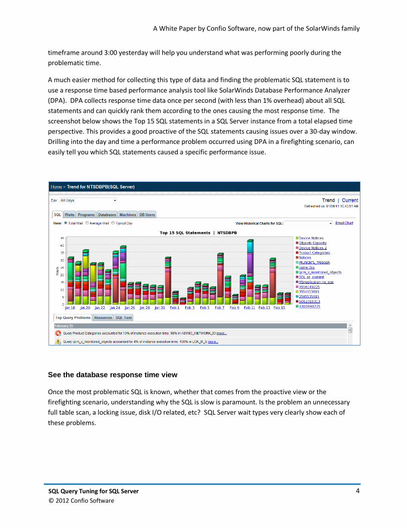
A much easier method for collecting this type of data and finding the problematic SQL statement is to
use a response time based performance analysis tool like SolarWinds Database Performance Analyzer
(DPA). DPA collects response time data once per second (with less than 1% overhead) about all SQL
statements and can quickly rank them according to the ones causing the most response time. The
screenshot below shows the Top 15 SQL statements in a SQL Server instance from a total elapsed time
perspective. This provides a good proactive of the SQL statements causing issues over a 30-day window.
Drilling into the day and time a performance problem occurred using DPA in a firefighting scenario, can
easily tell you which SQL statements caused a specific performance issue.
See the database response time view
Once the most problematic SQL is known, whether that comes from the proactive view or the
firefighting scenario, understanding why the SQL is slow is paramount. Is the problem an unnecessary
full table scan, a locking issue, disk I/O related, etc? SQL Server wait types very clearly show each of
these problems.
A White Paper by Confio Software, now part of the SolarWinds family
5 SQL Query Tuning for SQL Server
© 2012 Confio Software
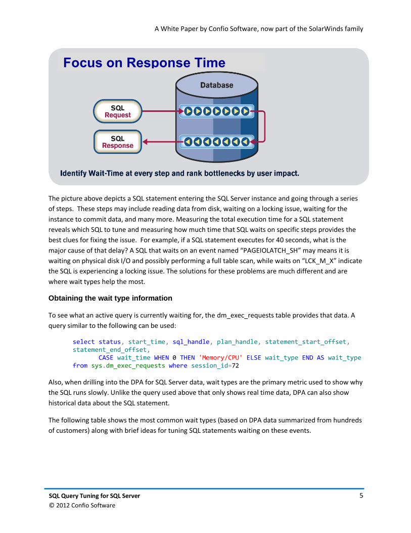
The picture above depicts a SQL statement entering the SQL Server instance and going through a series
of steps. These steps may include reading data from disk, waiting on a locking issue, waiting for the
instance to commit data, and many more. Measuring the total execution time for a SQL statement
reveals which SQL to tune and measuring how much time that SQL waits on specific steps provides the
best clues for fixing the issue. For example, if a SQL statement executes for 40 seconds, what is the
major cause of that delay? A SQL that waits on an event named “PAGEIOLATCH_SH” may means it is
waiting on physical disk I/O and possibly performing a full table scan, while waits on “LCK_M_X” indicate
the SQL is experiencing a locking issue. The solutions for these problems are much different and are
where wait types help the most.
Obtaining the wait type information
To see what an active query is currently waiting for, the dm_exec_requests table provides that data. A
query similar to the following can be used:
select status, start_time, sql_handle, plan_handle, statement_start_offset, statement_end_offset, CASE wait_time WHEN 0 THEN 'Memory/CPU' ELSE wait_type END AS wait_type from sys.dm_exec_requests where session_id=72
Also, when drilling into the DPA for SQL Server data, wait types are the primary metric used to show why
the SQL runs slowly. Unlike the query used above that only shows real time data, DPA can also show
historical data about the SQL statement.
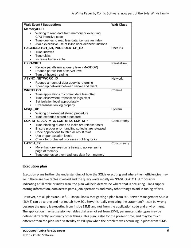
The following table shows the most common wait types (based on DPA data summarized from hundreds
of customers) along with brief ideas for tuning SQL statements waiting on these events.
Focus on Response Time
A White Paper by Confio Software, now part of the SolarWinds family
6 SQL Query Tuning for SQL Server
© 2012 Confio Software
Wait Event / Suggestions Wait Class
Memory/CPU
Waiting to read data from memory or executing CPU intensive code
Tune queries to read less data, i.e. use an index Avoid excessive use of inline user-defined functions
PAGEIOLATCH_SH, PAGEIOLATCH_EX User I/O
Tune indexes Tune disks Increase buffer cache
CXPACKET Parallelism
Reduce parallelism at query level (MAXDOP) Reduce parallelism at server level Turn off hyperthreading
ASYNC_NETWORK_IO Network
Reduce amount of data query is returning Speed up network between server and client
WRITELOG Commit
Tune applications to commit data less often Tune disks where transaction logs exist Set isolation level appropriately Size transaction log properly
MSQL_XP System
Waiting on extended stored procedure Tune extended stored procedure
LCK_M_S, LCK_M_X, LCK_M_IX, LCK_M_* Concurrency
Tune blocking queries so locks are release faster Ensure proper error handling so locks are released Code applications to fetch all result rows Use proper isolation levels Check for orphaned processes holding locks
LATCH_EX Concurrency
More than one session is trying to access same page of memory
Tune queries so they read less data from memory
Execution plan
Execution plans further the understanding of how the SQL is executing and where the inefficiencies may
lie. If there are five tables involved and the query waits mostly on “PAGEIOLATCH_SH” possibly
indicating a full table or index scan, the plan will help determine where that is occurring. Plans supply
costing information, data access paths, join operations and many other things to aid in tuning efforts.
However, not all plans are useful. Do you know that getting a plan from SQL Server Management Studio
(SSMS) can be wrong and not match how SQL Server is really executing the statement? It can be wrong
because the query is executing from inside SSMS and not from the application code and environment.
The application may set session variables that are not set from SSMS, parameter data types may be
defined differently, and many other things. This plan is also for the present time, and may be much
different than the plan used yesterday at 3:00 pm when the problem was occurring. If plans from SSMS
A White Paper by Confio Software, now part of the SolarWinds family
7 SQL Query Tuning for SQL Server
© 2012 Confio Software
can be wrong, where is a better place to retrieve the correct one? The best places to get execution plan
information are:
1. dm_exec_query_plan() or dm_exec_text_query_plan() – contains raw data for execution plans
of SQL statements. It provides the plan SQL Server used so why not go straight to the source.
Using dm_exec_query_plan from SSMS will provide a nice graphical view of the plan. To use this
DMO, pass in the plan_handle value from the query above against the dm_exec_requests DMV.
2. Tracing – provides great information as well as executions plans for a specific session, user or
the entire system.
3. Historical Data – if possible, collect and save execution plan information so you can go back to
3:00 pm yesterday to understand why the SQL statement performed poorly.
DPA for SQL Server collects execution plans in real time and associates them with the SQL statements,
wait types and other performance data. It is shown graphically with popup dialogs when mousing over
specific steps in the plan. DPA also keeps this data historically so you can go back to the problem at 3:00
pm to find exactly which plan was being used. Querying plans from the DMVs or getting them from
tracing will not provide this historical view.
Not all plans are created equal
Here is an example where, based on response time data, we believed the query was doing a full table
scan since the SQL was spending over 95% of its execution time waiting for PAGEIOLATCH_SH and the
logical and physical reads were very high per execution. However, when we reviewed the plan output
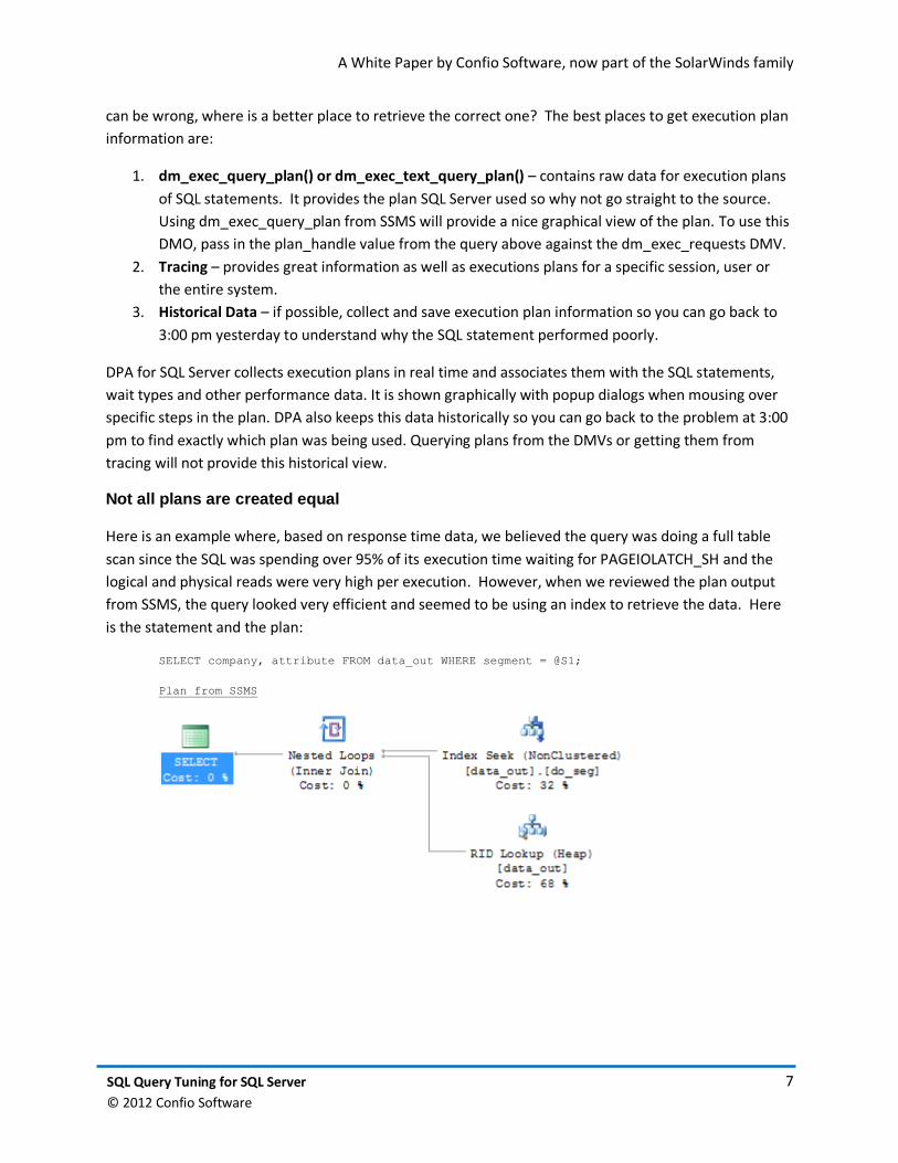
from SSMS, the query looked very efficient and seemed to be using an index to retrieve the data. Here
is the statement and the plan:
SELECT company, attribute FROM data_out WHERE segment = @S1;
Plan from SSMS
A White Paper by Confio Software, now part of the SolarWinds family
8 SQL Query Tuning for SQL Server
© 2012 Confio Software
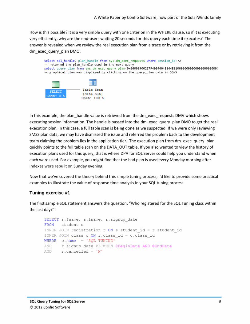
How is this possible? It is a very simple query with one criterion in the WHERE clause, so if it is executing
very efficiently, why are the end-users waiting 20 seconds for this query each time it executes? The
answer is revealed when we review the real execution plan from a trace or by retrieving it from the
dm_exec_query_plan DMO:
select sql_handle, plan_handle from sys.dm_exec_requests where session_id=72 -- returned the plan_handle used in the next query
select query_plan from sys.dm_exec_query_plan(0x06000900217F40094041844E010000000000000000000000) -- graphical plan was displayed by clicking on the query_plan data in SSMS
In this example, the plan_handle value is retrieved from the dm_exec_requests DMV which shows
executing session information. The handle is passed into the dm_exec_query_plan DMO to get the real
execution plan. In this case, a full table scan is being done as we suspected. If we were only reviewing
SMSS plan data, we may have dismissed the issue and referred the problem back to the development
team claiming the problem lies in the application tier. The execution plan from dm_exec_query_plan
quickly points to the full table scan on the DATA_OUT table. If you also wanted to view the history of
execution plans used for this query, that is where DPA for SQL Server could help you understand when
each were used. For example, you might find that the bad plan is used every Monday morning after
indexes were rebuilt on Sunday evening.
Now that we’ve covered the theory behind this simple tuning process, I’d like to provide some practical
examples to illustrate the value of response time analysis in your SQL tuning process.
Tuning exercise #1
The first sample SQL statement answers the question, “Who registered for the SQL Tuning class within
the last day?”:
SELECT s.fname, s.lname, r.signup_date
FROM student s
INNER JOIN registration r ON s.student_id = r.student_id
INNER JOIN class c ON r.class_id = c.class_id
WHERE c.name = 'SQL TUNING'
AND r.signup_date BETWEEN @BeginDate AND @EndDate
AND r.cancelled = 'N'
A White Paper by Confio Software, now part of the SolarWinds family
9 SQL Query Tuning for SQL Server
© 2012 Confio Software
Review execution plan and query statistics
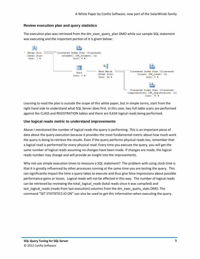
The execution plan was retrieved from the dm_exec_query_plan DMO while our sample SQL statement
was executing and the important portion of it is given below:
Learning to read the plan is outside the scope of this white paper, but in simple terms, start from the
right hand side to understand what SQL Server does first. In this case, two full table scans are performed
against the CLASS and REGISTRATION tables and there are 9,634 logical reads being performed.
Use logical reads metric to understand improvements
Above I mentioned the number of logical reads the query is performing. This is an important piece of
data about the query execution because it provides the most fundamental metric about how much work
the query is doing to retrieve the results. Even if the query performs physical reads too, remember that
a logical read is performed for every physical read. Every time you execute the query, you will get the
same number of logical reads assuming no changes have been made. If changes are made, the logical
reads number may change and will provide an insight into the improvements.
Why not use simple execution times to measure a SQL statement? The problem with using clock time is
that it is greatly influenced by other processes running at the same time you are testing the query. This
can significantly impact the time a query takes to execute and thus give false impressions about possible
performance gains or losses. Logical reads will not be affected in this way. The number of logical reads
can be retrieved by reviewing the total_logical_reads (total reads since it was compiled) and
last_logical_reads (reads from last execution) columns from the dm_exec_query_stats DMO. The
command “SET STATISTICS IO ON” can also be used to get this information when executing the query.
A White Paper by Confio Software, now part of the SolarWinds family
10 SQL Query Tuning for SQL Server
© 2012 Confio Software
SQL diagramming
I would like to introduce a technique to tune SQL statements correctly without the trial and error that I
was often faced with. The concept of SQL diagramming was introduced to me through a book entitled
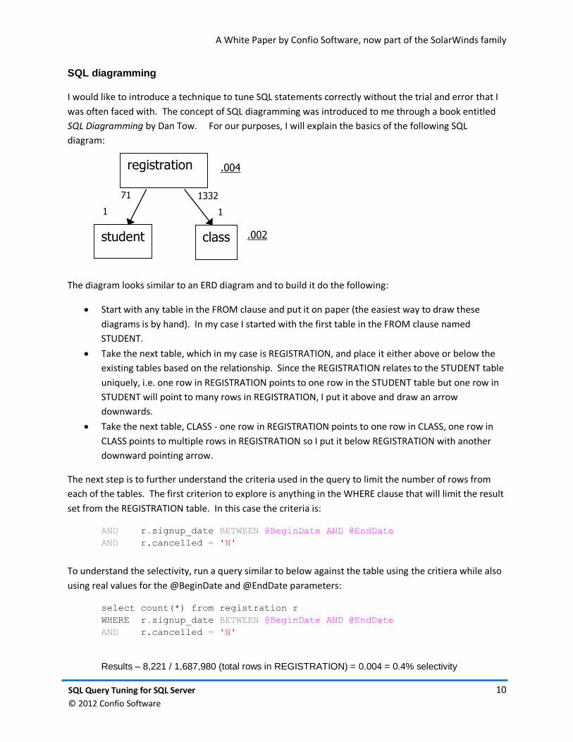
SQL Diagramming by Dan Tow. For our purposes, I will explain the basics of the following SQL
diagram:
The diagram looks similar to an ERD diagram and to build it do the following:
Start with any table in the FROM clause and put it on paper (the easiest way to draw these
diagrams is by hand). In my case I started with the first table in the FROM clause named
STUDENT.
Take the next table, which in my case is REGISTRATION, and place it either above or below the
existing tables based on the relationship. Since the REGISTRATION relates to the STUDENT table
uniquely, i.e. one row in REGISTRATION points to one row in the STUDENT table but one row in
STUDENT will point to many rows in REGISTRATION, I put it above and draw an arrow
downwards.
Take the next table, CLASS - one row in REGISTRATION points to one row in CLASS, one row in
CLASS points to multiple rows in REGISTRATION so I put it below REGISTRATION with another
downward pointing arrow.
The next step is to further understand the criteria used in the query to limit the number of rows from
each of the tables. The first criterion to explore is anything in the WHERE clause that will limit the result
set from the REGISTRATION table. In this case the criteria is:
AND r.signup_date BETWEEN @BeginDate AND @EndDate
AND r.cancelled = 'N'
To understand the selectivity, run a query similar to below against the table using the critiera while also
using real values for the @BeginDate and @EndDate parameters:
select count(*) from registration r
WHERE r.signup_date BETWEEN @BeginDate AND @EndDate
AND r.cancelled = 'N'
Results – 8,221 / 1,687,980 (total rows in REGISTRATION) = 0.004 = 0.4% selectivity
class .002 student
1
71
1
1332
.004 registration

A White Paper by Confio Software, now part of the SolarWinds family
11 SQL Query Tuning for SQL Server
© 2012 Confio Software
The query returned 8,221 rows and, with simple division by the total number of rows in the table, we
get a value of 0.004 or 0.4%. Place this number on the diagram next to the REGISTRATION table and
underline it. This represents the selectivity of the criteria against that table.
The next table to review in the same manner is the CLASS table. The query to run becomes:
SELECT count(1) FROM class
WHERE name = 'SQL TUNING'
Results – 2 / 1,267 (total rows in CLASS) = 0.001 = 0.1% selectivity
Place this in the diagram next to the CLASS table. The next table to explore is the STUDENT table, but
there are no direct criteria against this table, so no underlined number is placed next to that table.
The other numbers next to the arrows in the diagram are simple calculations based on average numbers
of rows that one row in a table references in the others. In this case, the REGISTRATION table refers to
exactly one row in the CLASS and STUDENT tables so the number 1 goes next to the bottom of the
arrows. One row in the CLASS table refers to on average 1,332 rows in the REGISTRATION table
(1,687,980 total rows REGISTRATION divided by 1,276 rows in CLASS) and one row in the STUDENT table
refers to on average 71 rows in REGISTRATION (1,687,980 / 23,768).
The diagram has now been completed for our example, however, Dan Tow goes into more detail than I
will include at this point.
Analyzing the SQL diagram
Analyzing the SQL diagram begins by looking for the criterion with the best selectivity or in the case of
this diagram, the smallest, underlined number. In this example it is 0.001 next to the CLASS table. To
limit the number of rows the query needs to process, starting here will trim our result sets the soonest.
If we can make SQL Server start with this table the query can be executed optimally. When the query
starts with the CLASS table for this query, it will read two rows and then visit the REGISTRATION table to
read 2,664 rows (2 * 1,332) – actually, this is the worst case because the criteria on the REGISTRATION
table would also be applied to limit the results. From there it will read 2,664 more rows from the CLASS
table for a total of 5,330 rows (2 + 2,664 + 2,664). If the query started on the REGISTRATION table first, it
would read 8,221 rows and then 8,221 rows from the CLASS and STUDENT tables for a total of 24,663
rows (3 * 8,221). Based on this data we can understand why starting on the CLASS table is best for this
query.
A White Paper by Confio Software, now part of the SolarWinds family
12 SQL Query Tuning for SQL Server
© 2012 Confio Software
Tuning based on SQL diagrams
We know we want the SQL Server optimizer to start with the CLASS table when executing this query, but
how do we do that? One way is to ensure an index exists and fits our criteria of “name = ‘SQL TUNING”.
In this case that means the NAME column of the CLASS table.
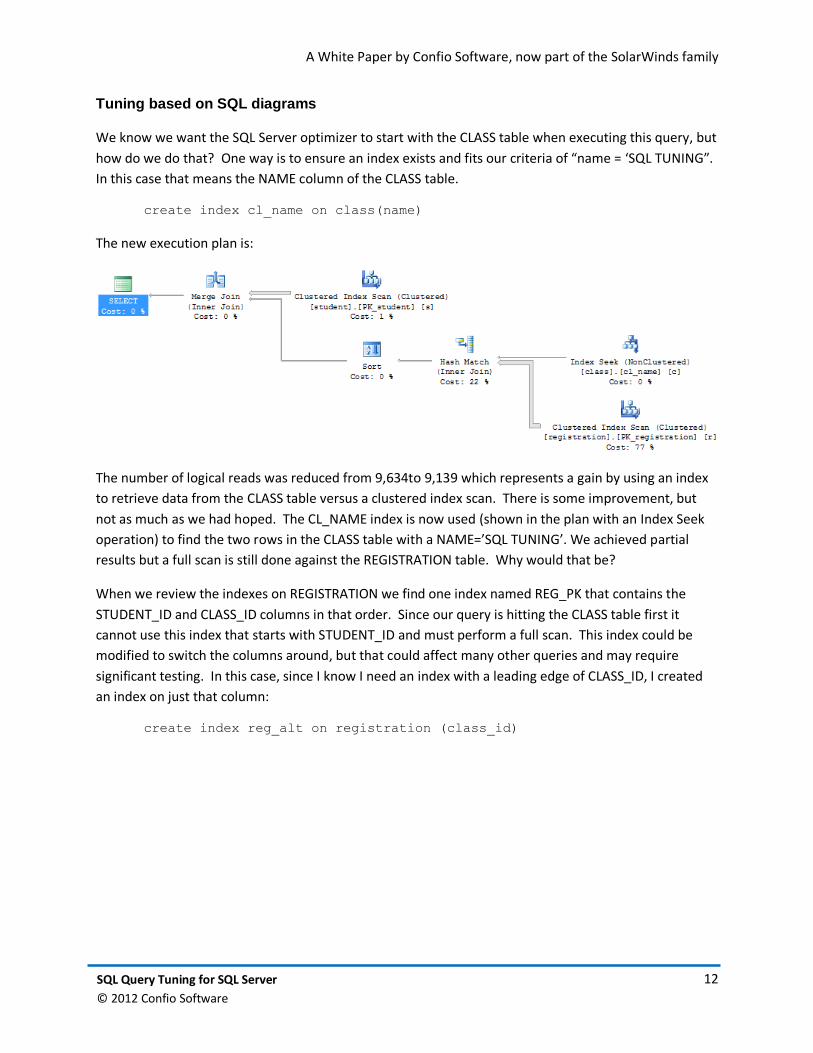
create index cl_name on class(name)
The new execution plan is:
The number of logical reads was reduced from 9,634to 9,139 which represents a gain by using an index
to retrieve data from the CLASS table versus a clustered index scan. There is some improvement, but
not as much as we had hoped. The CL_NAME index is now used (shown in the plan with an Index Seek
operation) to find the two rows in the CLASS table with a NAME=’SQL TUNING’. We achieved partial
results but a full scan is still done against the REGISTRATION table. Why would that be?
When we review the indexes on REGISTRATION we find one index named REG_PK that contains the
STUDENT_ID and CLASS_ID columns in that order. Since our query is hitting the CLASS table first it
cannot use this index that starts with STUDENT_ID and must perform a full scan. This index could be
modified to switch the columns around, but that could affect many other queries and may require
significant testing. In this case, since I know I need an index with a leading edge of CLASS_ID, I created
an index on just that column:
create index reg_alt on registration (class_id)
A White Paper by Confio Software, now part of the SolarWinds family
13 SQL Query Tuning for SQL Server
© 2012 Confio Software
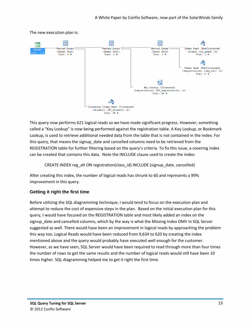
The new execution plan is:
This query now performs 621 logical reads so we have made significant progress. However, something
called a “Key Lookup” is now being performed against the registration table. A Key Lookup, or Bookmark
Lookup, is used to retrieve additional needed data from the table that is not contained in the index. For
this query, that means the signup_date and cancelled columns need to be retrieved from the
REGISTRATION table for further filtering based on the query’s criteria. To fix this issue, a covering index
can be created that contains this data. Note the INCLUDE clause used to create the index:
CREATE INDEX reg_alt ON registration(class_id) INCLUDE (signup_date, cancelled)
After creating this index, the number of logical reads has shrunk to 60 and represents a 99%
improvement in this query.
Getting it right the first time
Before utilizing the SQL diagramming technique, I would tend to focus on the execution plan and
attempt to reduce the cost of expensive steps in the plan. Based on the initial execution plan for this
query, I would have focused on the REGISTRATION table and most likely added an index on the
signup_date and cancelled columns, which by the way is what the Missing Index DMV in SQL Server
suggested as well. There would have been an improvement in logical reads by approaching the problem
this way too. Logical Reads would have been reduced from 9,634 to 620 by creating the index
mentioned above and the query would probably have executed well enough for the customer.
However, as we have seen, SQL Server would have been required to read through more than four times
the number of rows to get the same results and the number of logical reads would still have been 10
times higher. SQL diagramming helped me to get it right the first time.
A White Paper by Confio Software, now part of the SolarWinds family
14 SQL Query Tuning for SQL Server
© 2012 Confio Software
Tuning exercise #2
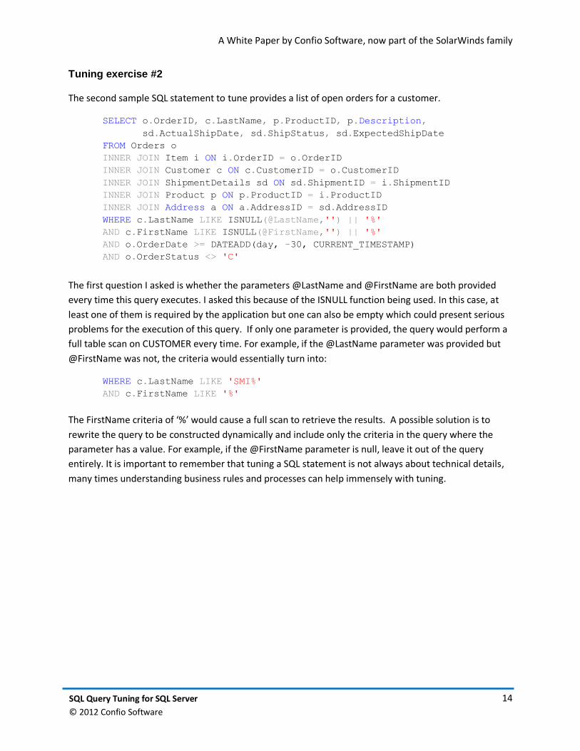
The second sample SQL statement to tune provides a list of open orders for a customer.
SELECT o.OrderID, c.LastName, p.ProductID, p.Description,
sd.ActualShipDate, sd.ShipStatus, sd.ExpectedShipDate
FROM Orders o
INNER JOIN Item i ON i.OrderID = o.OrderID
INNER JOIN Customer c ON c.CustomerID = o.CustomerID
INNER JOIN ShipmentDetails sd ON sd.ShipmentID = i.ShipmentID
INNER JOIN Product p ON p.ProductID = i.ProductID
INNER JOIN Address a ON a.AddressID = sd.AddressID
WHERE c.LastName LIKE ISNULL(@LastName,'') || '%'
AND c.FirstName LIKE ISNULL(@FirstName,'') || '%'
AND o.OrderDate >= DATEADD(day, -30, CURRENT_TIMESTAMP)
AND o.OrderStatus <> 'C'
The first question I asked is whether the parameters @LastName and @FirstName are both provided
every time this query executes. I asked this because of the ISNULL function being used. In this case, at
least one of them is required by the application but one can also be empty which could present serious
problems for the execution of this query. If only one parameter is provided, the query would perform a
full table scan on CUSTOMER every time. For example, if the @LastName parameter was provided but
@FirstName was not, the criteria would essentially turn into:
WHERE c.LastName LIKE 'SMI%'
AND c.FirstName LIKE '%'
The FirstName criteria of ‘%’ would cause a full scan to retrieve the results. A possible solution is to
rewrite the query to be constructed dynamically and include only the criteria in the query where the
parameter has a value. For example, if the @FirstName parameter is null, leave it out of the query
entirely. It is important to remember that tuning a SQL statement is not always about technical details,
many times understanding business rules and processes can help immensely with tuning.
A White Paper by Confio Software, now part of the SolarWinds family
15 SQL Query Tuning for SQL Server
© 2012 Confio Software
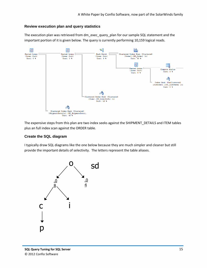
Review execution plan and query statistics
The execution plan was retrieved from dm_exec_query_plan for our sample SQL statement and the
important portion of it is given below. The query is currently performing 10,159 logical reads.
The expensive steps from this plan are two index seeks against the SHIPMENT_DETAILS and ITEM tables
plus an full index scan against the ORDER table.
Create the SQL diagram
I typically draw SQL diagrams like the one below because they are much simpler and cleaner but still
provide the important details of selectivity. The letters represent the table aliases.
o
.08
.04
i c
p
sd

A White Paper by Confio Software, now part of the SolarWinds family
16 SQL Query Tuning for SQL Server
© 2012 Confio Software
In this example, the end-users are trained to input only the first three characters of a name. Because of
this, when calculating selectivity for the CUSTOMER table we should use the most common 3 character
string found in the LastName and FirstName columns. In this example, “SMI%” is the most occurring first
three characters of the LASTNAME. Note, this data should not be assumed, but rather calculated from
the data and in our case there were a lot of Smiths.
SELECT COUNT(1) FROM Customer
WHERE LastName LIKE 'SMI%'
Results – 1,917 / 52,189 = .04
The next table to review is the ORDERS table. Whenever I have two criteria against a table in a query, I
calculate selectivity numbers for both combined as well as individually. I want to understand selectivity
of each to be able to create the best, most economical index. For this SQL statement I ran the following
queries:
SELECT count(1) FROM orders o
WHERE o.OrderDate >= SYSDATE - 30
AND o.OrderStatus <> 'C'
Combined Results – 0.005 = 0.5% selectivity
SELECT count(1) FROM orders o
WHERE o.OrderDate >= SYSDATE - 30
OrderDate Criteria Results – 0.08 = 8% selectivity
SELECT count(1) FROM orders o
WHERE o.OrderStatus <> 'C'
OrderStatus Criteria Results – 0.005 = 0.5% selectivity
These results show the ORDERDATE column selectivity is not near as good as the selectivity of the
ORDERSTATUS column individually. Also, when including both criteria, the selectivity matches the
results from using only the ORDERSTATUS column. Because of this, I would focus on that criterion alone
without ORDERDATE.
A White Paper by Confio Software, now part of the SolarWinds family
17 SQL Query Tuning for SQL Server
© 2012 Confio Software
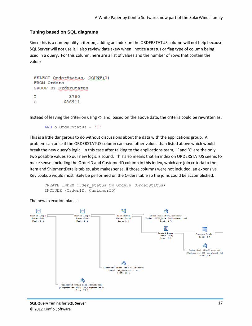
Tuning based on SQL diagrams
Since this is a non-equality criterion, adding an index on the ORDERSTATUS column will not help because
SQL Server will not use it. I also review data skew when I notice a status or flag type of column being
used in a query. For this column, here are a list of values and the number of rows that contain the
value:
Instead of leaving the criterion using <> and, based on the above data, the criteria could be rewritten as:
AND o.OrderStatus = 'I'
This is a little dangerous to do without discussions about the data with the applications group. A
problem can arise if the ORDERSTATUS column can have other values than listed above which would
break the new query’s logic. In this case after talking to the applications team, ‘I’ and ‘C’ are the only
two possible values so our new logic is sound. This also means that an index on ORDERSTATUS seems to
make sense. Including the OrderID and CustomerID column in this index, which are join criteria to the
Item and ShipmentDetails tables, also makes sense. If those columns were not included, an expensive
Key Lookup would most likely be performed on the Orders table so the joins could be accomplished.
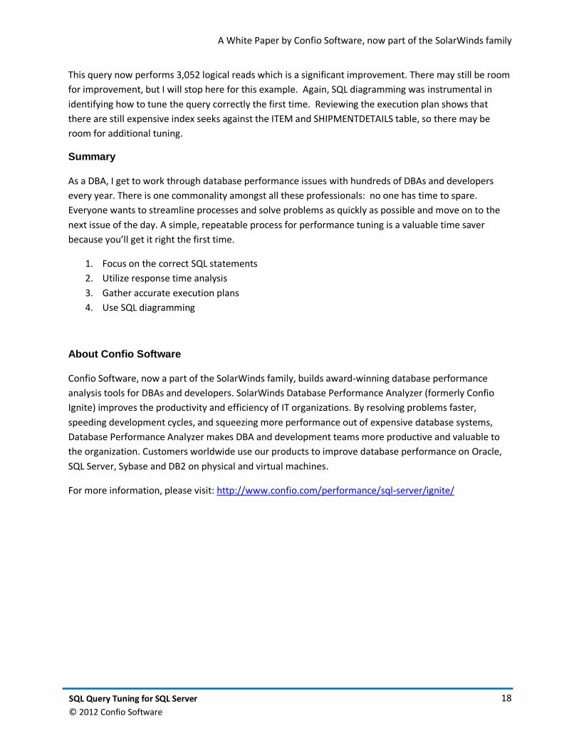
CREATE INDEX order_status ON Orders (OrderStatus)
INCLUDE (OrderID, CustomerID)
The new execution plan is:
A White Paper by Confio Software, now part of the SolarWinds family
18 SQL Query Tuning for SQL Server
© 2012 Confio Software
This query now performs 3,052 logical reads which is a significant improvement. There may still be room
for improvement, but I will stop here for this example. Again, SQL diagramming was instrumental in
identifying how to tune the query correctly the first time. Reviewing the execution plan shows that
there are still expensive index seeks against the ITEM and SHIPMENTDETAILS table, so there may be
room for additional tuning.
Summary
As a DBA, I get to work through database performance issues with hundreds of DBAs and developers
every year. There is one commonality amongst all these professionals: no one has time to spare.
Everyone wants to streamline processes and solve problems as quickly as possible and move on to the
next issue of the day. A simple, repeatable process for performance tuning is a valuable time saver
because you’ll get it right the first time.
1. Focus on the correct SQL statements
2. Utilize response time analysis
3. Gather accurate execution plans
4. Use SQL diagramming
About Confio Software
Confio Software, now a part of the SolarWinds family, builds award-winning database performance
analysis tools for DBAs and developers. SolarWinds Database Performance Analyzer (formerly Confio
Ignite) improves the productivity and efficiency of IT organizations. By resolving problems faster,
speeding development cycles, and squeezing more performance out of expensive database systems,
Database Performance Analyzer makes DBA and development teams more productive and valuable to
the organization. Customers worldwide use our products to improve database performance on Oracle,
SQL Server, Sybase and DB2 on physical and virtual machines.
For more information, please visit: http://www.confio.com/performance/sql-server/ignite/