What is database?

A collection of information organized in such a way that a computer program can quickly select desired pieces of data. You can think of a database as an electronic filing system.

In other words,

A database provides a systematic and organized way of storing, managing, and retrieving desired information from the collection of logically related information.A database should be persistent and it should provide an independent way of accessing data without the dependency of any application. SQL Server is an RDBMS.

What is the difference between DBMS (Database Management System) and RDBMS (Relational Database Management System)?

DBMS stands for Database Management System which is a general term for a set of software dedicated to controlling the storage of data. RDMBS stand for Relational Database Management System. This is the most common form of DBMS.

RDBMS=DBMS + Relationship

An RDBMS is a Relational Data Base Management System. This adds the additional condition that the system supports a tabular structure for the data, with enforced relationships between the tables. In DBMS all the tables are treated as different entities. There is no relation established among these entities. But the tables in RDBMS are dependent and the user can establish various integrity constraints on these tables so that the ultimate data used by the user remains correct.

In DBMS there are entity sets in the form of tables but relationship among them is not defined while in RDBMS in each entity is well defined with a relationship set so as retrieve our data fast and easy.

There is a big diff. between DBMS and RDBMS. 1) For a DBMS to be titled as a RDBMS, it must follow the Code’s rules (atlest 6 of 12)

2) Integrity rules can not be applied on a DBMS  (Without a very complex piece of code ) while an RDBMS provides Primary/Foreign Key constraints for this purpose. With the help of these constraints we are able to establish a relation betwen 2 or more tables or even databases and thus this known as Relational DBMS.

3)  DBMS are for smaller organizations with small amount of data, where security of the data is not of major concern. Also DBMS are not necessarily client server based systems. With DBMS, one can develop a complete application, starting from processing inputs to generating output.

RDBMS are designed to take care of large amounts of data and also the security of this data. They are also client server based systems. To create a complete application, one requires client software like VB, Developer 2000.FoxPro data files and earlier Ms Access are DBMSSQL Server, Oracle, DB2, Sybase are RDBMS

Referential Integrity:Referential integrity refers to the relationship between tables. Because each table in a database must have a primary key, this primary key can appear in other tables because of its relationship to data within those tables. When a primary key from one table appears in another table, it is called a foreign key.Foreign keys join tables and establish dependencies between tables.

1

Referential integrity is the logical dependency of a foreign key on a primary key. The integrity of a row that contains a foreign key depends on the integrity of the row that it references—the row that contains the matching primary key.By default, the database server does not allow you to violate referential integrity and gives you an error message if you attempt to delete rows from the parent table before you delete rows from the child table. You can, however, use the ON DELETE CASCADE option to cause deletes from a parent table to trip deletes on child tables.

To maintain referential integrity when you delete rows from a primary key for a table, use the ON DELETE CASCADE option in the REFERENCES clause of the CREATE TABLE and ALTER TABLE statements. This option allows you to delete a row from a parent table and its corresponding rows in matching child tables with a single delete command.

If you have a parent table with two child constraints, one child with cascading deletes specified and one child without cascading deletes, and you attempt to delete a row from the parent table that applies to both child tables, the DELETE statement fails, and no rows are deleted from either the parent or child tables.

Important:

You cannot define a DELETE trigger event on a table if all the tables don’t define a referential constraint with ON DELETE CASCADE.

Difference in MS Access and MS SQL Server:Data Difference

Access SQL Server SQL Server Definition Yes/No BIT (Integer: 0 or 1)

Number (Byte) TINYINT (Positive Integer 0 -> 255)

Number (Integer) SMALLINT (Signed Integer -32,768 -> 32,767)

Number (Long Integer) INT (Signed Integer -(2^31) -> (2^31)-1)

(no equivalent) BIGINT (Signed Integer -(2^63) -> (2^63)-1)

Number (Single) REAL (Floating precision -1.79E + 308)

Number (Double) FLOAT (Floating precision -3.40E + 38)

Currency MONEY (4 decimal places with big number)

Currency SMALLMONEY (4 decimal places small number)

Hyperlink (no equivalent) Use VARCHAR())

Decimal DECIMAL (Fixed precision -10^38 + 1 -> 10^38 - 1)

Date/Time DATETIME

Text(n) CHAR(n) (Fixed-length string to 8,000 characters)

Text(n) VARCHAR(n) (Variable-length string to 8,000 characters)

Text(n) NVARCHAR(n) (Variable-length to 4,000 characters)

Memo TEXT (Variable-length string to 2,147,483,647

Chars)

OLE Object BINARY (Fixed-length binary data up to 8,000 Chars)

OLE Object IMAGE (Variable-length binary data )

Autonumber

Autoincrement IDENTITY (any numeric data type, with IDENTITY

property)

Autonumber to IDENTITY with DDL (CREATE TABLE) statements:  

2

Access: CREATE TABLE tablename (id AUTOINCREMENT) 

-- SQL Server: CREATE TABLE tablename (id INT IDENTITY)Handling Strings Concatinating String :

-- Access: SELECT FirstName & ' ' & LastName FROM table

-- SQL Server: SELECT FirstName + ' ' + LastName FROM table

String Functions :

There are many VBA-based functions in Access which are used to manipulate strings. Some of these functions are still supported in SQL Server.

Access SQL Server CINT(), CLNG() CAST()

FORMAT() CONVERT()

INSTR() CHARINDEX()

ISDATE() ISDATE()

ISNULL() ISNULL()

ISNUMERIC() ISNUMERIC()

LEFT() LEFT()

LEN() LEN()

LCASE() LOWER()

LTRIM() LTRIM()

REPLACE() REPLACE()

RIGHT() RIGHT()

RTRIM() RTRIM()

CSTR() STR()

MID() SUBSTRING()

UCASE() UPPER()

StrConv() n/a

TRIM() n/a

 CINT(data) -> CAST(data AS INT) This function converts NUMERIC data that may be stored in string format to INTEGER format for comparison and computation -- Access: SELECT CINT(column) -- SQL Server: SELECT CAST(column AS INT)INSTR(data, expression) -> CHARINDEX(expression, data) This function returns an integer representing the character where the search expression is found within the data parameter. Note that the order of these parameters is reversed!  -- Access: SELECT INSTR("franky goes to hollywood","goes")

3

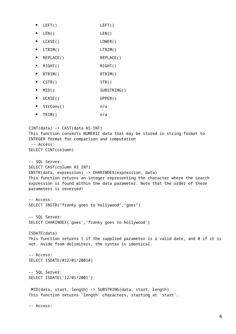
-- SQL Server: SELECT CHARINDEX('goes','franky goes to hollywood') ISDATE(data) This function returns 1 if the supplied parameter is a valid date, and 0 if it is not. Aside from delimiters, the syntax is identical.  -- Access: SELECT ISDATE(#12/01/2001#) -- SQL Server: SELECT ISDATE('12/01/2001')

 MID(data, start, length) -> SUBSTRING(data, start, length) This function returns 'length' characters, starting at 'start'.  -- Access: SELECT MID("franky goes to hollywood",1,6) -- SQL Server: SELECT SUBSTRING('franky goes to hollywood',1,6)UCASE(data) -> UPPER(data) This function converts data to upper case.  TRIM(data) This function combines both LTRIM() and LTRIM(); there is no equivalent in SQL Server. To mimic the functionality, you would combine the two functions:  -- Access: SELECT TRIM(column) SELECT LTRIM(RTRIM(column)) -- SQL Server: SELECT LTRIM(RTRIM(column))

IIF(expression, resultIftrue, resultIfFalse)

IIF() is a handy inline switch comparison, which returns one result if the expression is true, and another result if the expression is false. IIF() is a VBA function, and as such, is not available in SQL Server. Thankfully, there is a more powerful function in SQL Server, called CASE. It operates much like SELECT CASE in Visual Basic. Here is an example query: 

-- Access: SELECT IIF(Column<>0, "Yes", "No") as Col FROM table -- SQL Server: SELECT col2=CASE WHEN Col2='a' THEN 'US' WHEN Col2='b' THEN 'Canada' ELSE 'Foreign' END FROM table Difference in other aspects:

Access uses file server design where as SQL Server uses client server

model.

Access Database cannot contain more then 2 GB data

SQL Server can contain in terabytes

SQL Server can provide access to thousands of users

4

Access Database provide access to 5 to 8 of users

SECURITY Access is limited to security in terms of username / password on the database. It also is subject to Windows security on the file itself (as well as the folder it resides in).

SQL Server has two authentication modes, and neither are much like Access security at all. You can use Windows Authentication, which allows you direct access to domain Users and Groups from within the interface. You can also use Mixed Mode, which allows SQL Server to maintain usernames and passwords. Once you have determined an authentication mode, users have three different levels of access into the database: login (at the server level), user (at the database level), and object permissions within each database (for tables, views, stored procedures, etc). Just to add a layer of complexity, SQL Server makes it easy to "clone" users by defining server-wide roles, and adding users to that role. This is much like a Group in a Windows domain; in SQL Server, you can use the built-in definitions (and customize them), or create your own. Alterations to a role's permissions affect all users that are members of that role. 

SQL Server is a more robust database management system. SQL Server was designed to have many hundreds, or even thousands of users accessing it at any point in time. Microsoft Access on the other hand, doesn't handle this type of load very well.SQL Server also contains some advanced database administration tools that enable organisations to schedule tasks, receive alerts, optimize databases, configure security accounts/roles, transfer data between other disparate sources, and much more.

Steps of LearningKey:A key in a database table is a special column or a group of columns that uniquely identifies a row, defines the relationship, or is used to build an index.

Types of key:

Candidate Key

Primary Key (single column / composite column)

Alternate Key

Unique Key

Foreign Key (single column / composite column)

Surrogate Key / Synthetic Key

Natural Key

Candidate Key:A Candidate Key can be any column or a combination of columns that can qualify as unique key in database table. There can be multiple Candidate Keys in one table. Each Candidate Key can qualify as Primary Key.

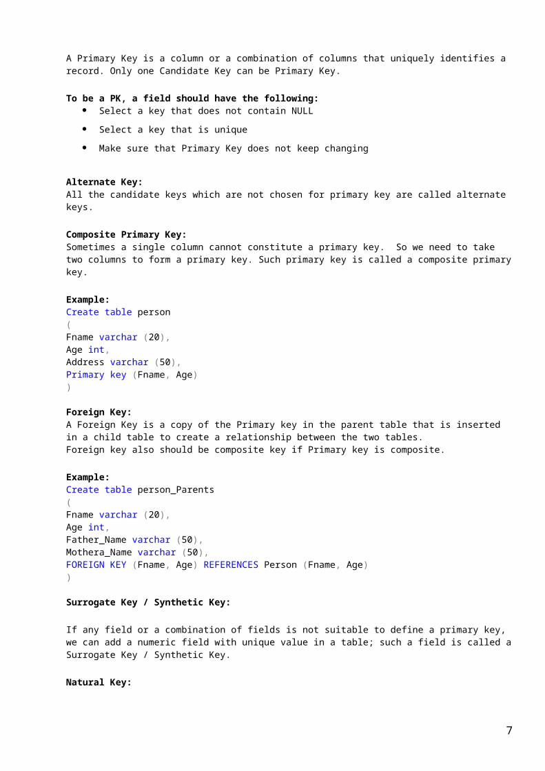
Primary Key:A Primary Key is a column or a combination of columns that uniquely identifies a record. Only one Candidate Key can be Primary Key.

To be a PK, a field should have the following: Select a key that does not contain NULL

Select a key that is unique

Make sure that Primary Key does not keep changing

5

Alternate Key:All the candidate keys which are not chosen for primary key are called alternate keys.

Composite Primary Key:Sometimes a single column cannot constitute a primary key. So we need to take two columns to form a primary key. Such primary key is called a composite primary key.

Example:Create table person( Fname varchar (20),Age int,Address varchar (50),Primary key (Fname, Age))

Foreign Key:A Foreign Key is a copy of the Primary key in the parent table that is inserted in a child table to create a relationship between the two tables.Foreign key also should be composite key if Primary key is composite.

Example:Create table person_Parents( Fname varchar (20),Age int,Father_Name varchar (50),Mothera_Name varchar (50),FOREIGN KEY (Fname, Age) REFERENCES Person (Fname, Age))

Surrogate Key / Synthetic Key:

If any field or a combination of fields is not suitable to define a primary key, we can add a numeric field with unique value in a table; such a field is called a Surrogate Key / Synthetic Key.

Natural Key:

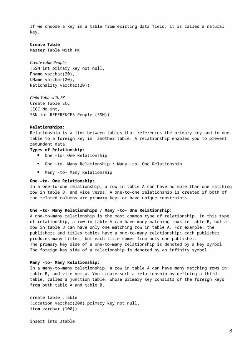
If we choose a key in a table from existing data field, it is called a natural key.

Create TableMaster Table with PK

Create table People(SSN int primary key not null,Fname varchar(20),LName varchar(20),Nationality varchar(20))

Child Table with FKCreate Table ECC(ECC_No int,SSN int REFERENCES People (SSN)) Relationships:Relationship is a link between tables that references the primary key and in one table to a foreign key in another table. A relationship enables you to prevent redundant data.Types of Relationship:

One –to- One Relationship

6

One –to- Many Relationship / Many –to- One Relationship

Many –to- Many Relationship

One –to- One Relationship:In a one-to-one relationship, a row in table A can have no more than one matching row in table B, and vice versa. A one-to-one relationship is created if both of the related columns are primary keys or have unique constraints.

One –to- Many Relationships / Many –to- One Relationship:A one-to-many relationship is the most common type of relationship. In this type of relationship, a row in table A can have many matching rows in table B, but a row in table B can have only one matching row in table A. For example, the publishers and titles tables have a one-to-many relationship: each publisher produces many titles, but each title comes from only one publisher.The primary key side of a one-to-many relationship is denoted by a key symbol. The foreign key side of a relationship is denoted by an infinity symbol.

Many –to- Many Relationship:In a many-to-many relationship, a row in table A can have many matching rows in table B, and vice versa. You create such a relationship by defining a third table, called a junction table, whose primary key consists of the foreign keys from both table A and table B.

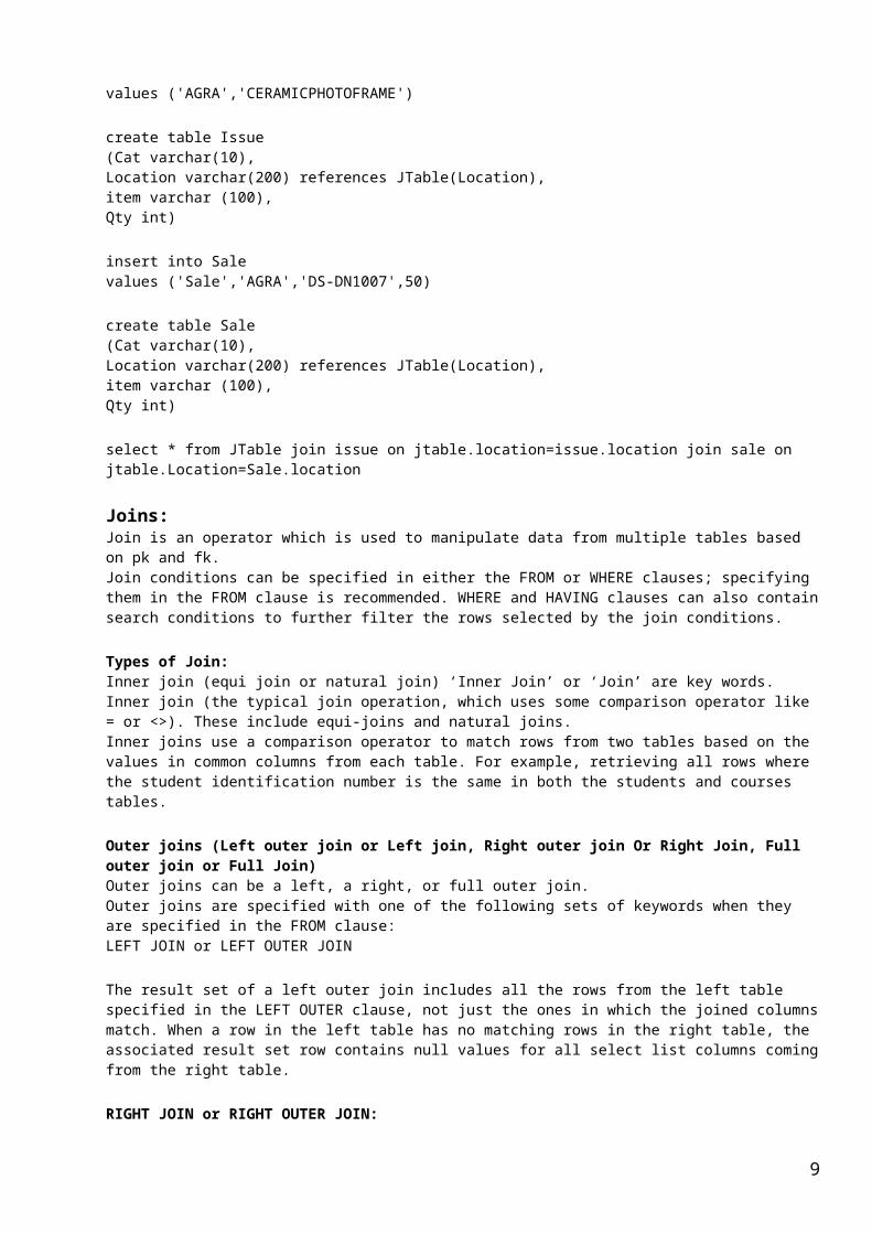
create table JTable(Location varchar(200) primary key not null,item varchar (100))

insert into Jtablevalues ('AGRA','CERAMICPHOTOFRAME')

create table Issue(Cat varchar(10),Location varchar(200) references JTable(Location),item varchar (100),Qty int)

insert into Salevalues ('Sale','AGRA','DS-DN1007',50)

create table Sale(Cat varchar(10),Location varchar(200) references JTable(Location),item varchar (100),Qty int)

select * from JTable join issue on jtable.location=issue.location join sale on jtable.Location=Sale.location

Joins:Join is an operator which is used to manipulate data from multiple tables based on pk and fk.Join conditions can be specified in either the FROM or WHERE clauses; specifying them in the FROM clause is recommended. WHERE and HAVING clauses can also contain search conditions to further filter the rows selected by the join conditions.

Types of Join:Inner join (equi join or natural join) ‘Inner Join’ or ‘Join’ are key words.Inner join (the typical join operation, which uses some comparison operator like = or <>). These include equi-joins and natural joins. Inner joins use a comparison operator to match rows from two tables based on the values in common columns from each table. For example, retrieving all rows where the student identification number is the same in both the students and courses tables.

7

Outer joins (Left outer join or Left join, Right outer join Or Right Join, Full outer join or Full Join)Outer joins can be a left, a right, or full outer join. Outer joins are specified with one of the following sets of keywords when they are specified in the FROM clause: LEFT JOIN or LEFT OUTER JOIN

The result set of a left outer join includes all the rows from the left table specified in the LEFT OUTER clause, not just the ones in which the joined columns match. When a row in the left table has no matching rows in the right table, the associated result set row contains null values for all select list columns coming from the right table.

RIGHT JOIN or RIGHT OUTER JOIN:A right outer join is the reverse of a left outer join. All rows from the right table are returned. Null values are returned for the left table any time a right table row has no matching row in the left table.

FULL JOIN or FULL OUTER JOIN:A full outer join returns all rows in both the left and right tables. Any time a row has no match in the other table, the select list columns from the other table contain null values. When there is a match between the tables, the entire result set row contains data values from the base tables.

select a.ProductID, a.Name,b.Quantityfrom Production.Product a full outer join Production.ProductInventory bon a.ProductID=b.ProductID

Cross joins:Cross joins return all rows from the left table. Each row from the left table is combined with all rows from the right table. Cross joins are also called Cartesian products.

select * from Production.Product cross join Production.ProductInventory

Self Join:A table can be joined to itself in a self-join. For example, you can use a self-join to find the products that are supplied by more than one vendor.

Because this query involves a join of the ProductVendor table with itself, the ProductVendor table appears in two roles. To distinguish these roles, you must give the ProductVendor table two different aliases (pv1 and pv2) in the FROM clause. These aliases are used to qualify the column names in the rest of the query. This is an example of the self-join Transact-SQL statement:

SELECT DISTINCT pv1.ProductID, pv1.VendorIDFROM Purchasing.ProductVendor pv1INNER JOIN Purchasing.ProductVendor pv2ON pv1.ProductID = pv2.ProductID AND pv1.VendorID <> pv2.VendorIDORDER BY pv1.ProductID

Note:

The previous examples specified the join conditions in the FROM clause, which is the preferred method. The following query contains the same join condition specified in the WHERE clause:

SELECT pv.ProductID, v.VendorID, v.NameFROM Purchasing.ProductVendor pv, Purchasing.Vendor vWHERE pv.VendorID = v.VendorID AND StandardPrice > $10

8

AND Name LIKE N'F%'

1. Simple query

Processing Order of the SELECT statement (FROM, where and select)

The following steps show the processing order for a SELECT statement.Select

FROM

ON

JOIN

WHERE

GROUP BY

WITH CUBE or WITH ROLLUP

HAVING

SELECT

DISTINCT

ORDER BY

TOP

Using SELECT to retrieve all rows and all columns:

SELECT *FROM Production.ProductORDER BY Name Desc

This query returns all rows (no WHERE clause is specified), and only a subset of the columns (Name, ProductNumber, ListPrice) from the Product table in the AdventureWorks database. Additionally, a column heading is added.

SELECT Name, ProductNumber, ListPrice AS PriceFROM Production.Product ORDER BY Name ASC

This query returns only the rows for Product that have a product line of R and that have days to manufacture that is less than 4:

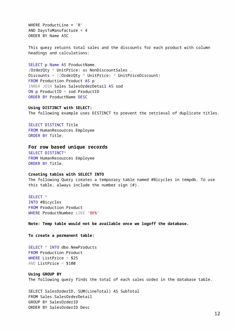
SELECT Name, ProductNumber, ListPrice AS PriceFROM Production.Product WHERE ProductLine = 'R' AND DaysToManufacture < 4ORDER BY Name ASC

This query returns total sales and the discounts for each product with column headings and calculations:

SELECT p.Name AS ProductName, (OrderQty * UnitPrice) as NonDiscountSales ,Discounts = ((OrderQty * UnitPrice) * UnitPriceDiscount)FROM Production.Product AS p INNER JOIN Sales.SalesOrderDetail AS sodON p.ProductID = sod.ProductID ORDER BY ProductName DESC

9

Using DISTINCT with SELECT:The following example uses DISTINCT to prevent the retrieval of duplicate titles.

SELECT DISTINCT TitleFROM HumanResources.EmployeeORDER BY Title;

For row based unique recordsSELECT DISTINCT*FROM HumanResources.EmployeeORDER BY Title;

Creating tables with SELECT INTO The following Query creates a temporary table named #Bicycles in tempdb. To use this table, always include the number sign (#).

SELECT * INTO #BicyclesFROM Production.ProductWHERE ProductNumber LIKE 'BK%'

Note: Temp table would not be available once we logoff the database.

To create a permanent table:

SELECT * INTO dbo.NewProductsFROM Production.ProductWHERE ListPrice > $25 AND ListPrice < $100

Using GROUP BY The following query finds the total of each sales order in the database table.

SELECT SalesOrderID, SUM(LineTotal) AS SubTotalFROM Sales.SalesOrderDetailGROUP BY SalesOrderIDORDER BY SalesOrderID Desc

Using GROUP BY with multiple groups The following Query finds the average price and the sum of year-to-date sales, grouped by product ID and special offer ID.

SELECT ProductID, SpecialOfferID, AVG(UnitPrice) AS 'Average Price', SUM(LineTotal) AS SubTotalFROM Sales.SalesOrderDetailGROUP BY ProductID, SpecialOfferIDORDER BY ProductID

Using GROUP BY and WHERE The following query puts the results into groups after retrieving only the rows with list prices greater than $1000.SELECT ProductModelID, AVG(ListPrice) AS 'Average List Price'FROM Production.ProductWHERE ListPrice > $1000GROUP BY ProductModelIDORDER BY ProductModelID

Using GROUP BY with an expression The following query groups by an expression. You can group by an expression if the expression does not include aggregate functions.

SELECT NonDiscountSales = (OrderQty * UnitPrice),AVG(OrderQty) AS 'Average Quantity'

10

FROM Sales.SalesOrderDetailGROUP BY (OrderQty * UnitPrice)ORDER BY (OrderQty * UnitPrice) DESC

Using Aggregate function with ORDER BY The following example finds the average price of each type of product and orders the results by average price.

SELECT ProductID, AVG(UnitPrice) AS 'Average Price'FROM Sales.SalesOrderDetailWHERE OrderQty > 10GROUP BY ProductIDORDER BY AVG(UnitPrice)

Using the HAVING clause The query shows a HAVING clause with an aggregate function. It groups the rows in the SalesOrderDetail table by product ID and eliminates products whose average order quantities are five or less.

Aggregate function with having clause

SELECT ProductID ,AVG(OrderQty) as qtyFROM Sales.SalesOrderDetailGROUP BY ProductIDHAVING AVG(OrderQty) > 5ORDER BY ProductID;

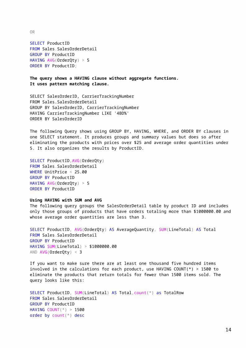
OR

SELECT ProductID FROM Sales.SalesOrderDetailGROUP BY ProductIDHAVING AVG(OrderQty) > 5 ORDER BY ProductID;

The query shows a HAVING clause without aggregate functions. It uses pattern matching clause.

SELECT SalesOrderID, CarrierTrackingNumber FROM Sales.SalesOrderDetailGROUP BY SalesOrderID, CarrierTrackingNumberHAVING CarrierTrackingNumber LIKE '4BD%'ORDER BY SalesOrderID

The following Query shows using GROUP BY, HAVING, WHERE, and ORDER BY clauses in one SELECT statement. It produces groups and summary values but does so after eliminating the products with prices over $25 and average order quantities under 5. It also organizes the results by ProductID.

SELECT ProductID,AVG(OrderQty)FROM Sales.SalesOrderDetailWHERE UnitPrice < 25.00GROUP BY ProductIDHAVING AVG(OrderQty) > 5ORDER BY ProductID

Using HAVING with SUM and AVGThe following query groups the SalesOrderDetail table by product ID and includes only those groups of products that have orders totaling more than $1000000.00 and whose average order quantities are less than 3.

SELECT ProductID, AVG(OrderQty) AS AverageQuantity, SUM(LineTotal) AS TotalFROM Sales.SalesOrderDetailGROUP BY ProductID

11

HAVING SUM(LineTotal) > $1000000.00AND AVG(OrderQty) < 3

If you want to make sure there are at least one thousand five hundred items involved in the calculations for each product, use HAVING COUNT(*) > 1500 to eliminate the products that return totals for fewer than 1500 items sold. The query looks like this:

SELECT ProductID, SUM(LineTotal) AS Total,count(*) as TotalRow FROM Sales.SalesOrderDetailGROUP BY ProductID HAVING COUNT(*) > 1500order by count(*) desc

Compute and Compute by Clause:

The compute clause is a SQL extension. Use it with row aggregates to produce reports that show subtotals of grouped summaries. Such reports, usually produced by a report generator, are called control-break reports, since summary values appear in the report under the control of the groupings ("breaks") you specify in the compute clause with BY key word.

Compute clause generates totals that appear as additional summary columns at the end of the result set. When used with BY, the COMPUTE clause generates control-breaks and subtotals in the result set.The row aggregates you can use with compute are sum, avg, min, max, and count.Compute and Compute by Clauses come after order by clause.

A COMPUTE BY clause allows you to see both detail and summary rows with one SELECT statement. You can calculate summary values for subgroups with compute …..By, or a summary value for the whole result set with Compute without by clause.

The summary values generated by COMPUTE appear as separate result sets in the query results. The results of a query that include a COMPUTE clause are like a control-break report. This is a report whose summary values are controlled by the groupings, or breaks, that you specify. You can produce summary values for groups, and you can also calculate more than one aggregate function for the same group.

The first result set for each group has the set of detail rows that contain the select list information for that group.

The second result set for each group has one row that contains the subtotals of the aggregate functions specified in the COMPUTE clause for that group.When COMPUTE is specified without the optional BY clause, there are two result sets for the SELECT:

The first result set for each group has all the detail rows that contain the select list information.

The second result set has one row that contains the totals of the aggregate functions specified in the COMPUTE clause.

The COMPUTE clause takes the following information:

The optional BY keyword: This calculates the specified row aggregate on a per column basis.

A row aggregate function name: This includes SUM, AVG, MIN, MAX, or COUNT.

A column upon which to perform the row aggregate function

Using COMPUTE in query to return totals

12

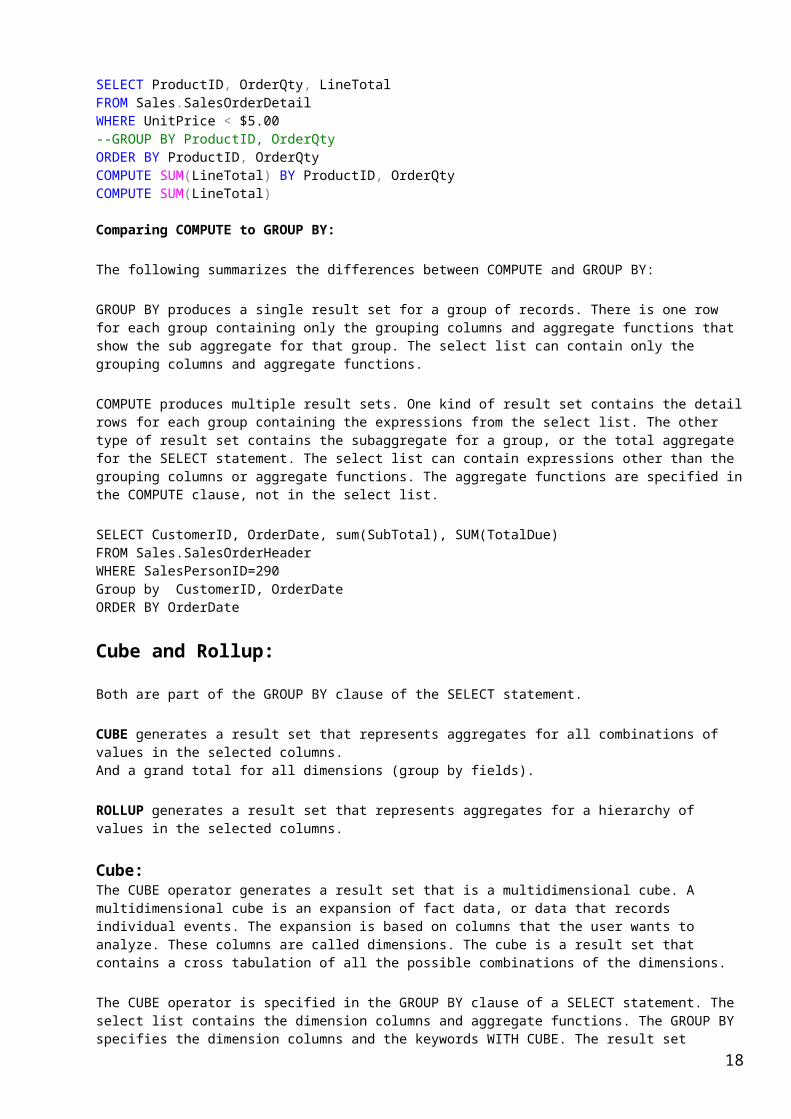
In the following example, the SELECT statement uses a simple COMPUTE clause to produce a grand total of the sum of the SubTotal and TotalDue from the SalesOrderHeader table.

SELECT CustomerID, OrderDate, SubTotal, TotalDueFROM Sales.SalesOrderHeaderWHERE SalesPersonID=290ORDER BY OrderDateCOMPUTE SUM(SubTotal), SUM(TotalDue)--COMPUTE SUM(SubTotal), SUM(TotalDue) by OrderDate

Compute ….by clause with multiple fieldsSELECT CustomerID, OrderDate, SalesPersonID,SubTotal, TotalDueFROM Sales.SalesOrderHeader--WHERE SalesPersonID=290ORDER BY OrderDate,SalesPersonID--COMPUTE SUM(SubTotal), SUM(TotalDue)COMPUTE SUM(SubTotal), SUM(TotalDue) by OrderDate,SalesPersonID

The following query uses both compute and compute by clause to produce the sub total and grand total.

SELECT CustomerID, OrderDate, SubTotal, TotalDueFROM Sales.SalesOrderHeaderWHERE SalesPersonID=290ORDER BY OrderDateCOMPUTE SUM(SubTotal), SUM(TotalDue)COMPUTE SUM(SubTotal), SUM(TotalDue) by OrderDate

Rules of compute and compute by clause:

1. You cannot use COMPUTE in a SELECT INTO statement because statements including COMPUTE generate tables and their summary results are not stored in the database. Therefore, any calculations produced by COMPUTE do not appear in the new table created with the SELECT INTO statement.

2. You cannot use the COMPUTE clause when the SELECT statement is part of a DECLARE CURSOR statement.

3. The DISTINCT keyword cannot be used with the aggregate functions.

4. All columns referred to in the COMPUTE clause must appear in the SELECT column list.

5. The ORDER BY clause must be used whenever the COMPUTE BY clause is used.

6. The ORDER BY clause can be eliminated only when the COMPUTE clause is used.

7. The columns listed in the COMPUTE BY clause must match the columns used in the ORDER BY clause (compute by clause cannot be used without order by clause).

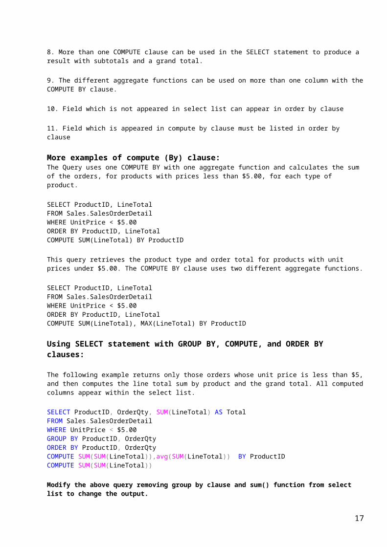
8. More than one COMPUTE clause can be used in the SELECT statement to produce a result with subtotals and a grand total.

9. The different aggregate functions can be used on more than one column with the COMPUTE BY clause.

10. Field which is not appeared in select list can appear in order by clause

11. Field which is appeared in compute by clause must be listed in order by clause

More examples of compute (By) clause:13

The Query uses one COMPUTE BY with one aggregate function and calculates the sum of the orders, for products with prices less than $5.00, for each type of product.

SELECT ProductID, LineTotalFROM Sales.SalesOrderDetailWHERE UnitPrice < $5.00ORDER BY ProductID, LineTotalCOMPUTE SUM(LineTotal) BY ProductID

This query retrieves the product type and order total for products with unit prices under $5.00. The COMPUTE BY clause uses two different aggregate functions.

SELECT ProductID, LineTotalFROM Sales.SalesOrderDetailWHERE UnitPrice < $5.00ORDER BY ProductID, LineTotalCOMPUTE SUM(LineTotal), MAX(LineTotal) BY ProductID

Using SELECT statement with GROUP BY, COMPUTE, and ORDER BY clauses:

The following example returns only those orders whose unit price is less than $5, and then computes the line total sum by product and the grand total. All computed columns appear within the select list.

SELECT ProductID, OrderQty, SUM(LineTotal) AS TotalFROM Sales.SalesOrderDetailWHERE UnitPrice < $5.00GROUP BY ProductID, OrderQtyORDER BY ProductID, OrderQtyCOMPUTE SUM(SUM(LineTotal)),avg(SUM(LineTotal)) BY ProductIDCOMPUTE SUM(SUM(LineTotal))

Modify the above query removing group by clause and sum() function from select list to change the output.

SELECT ProductID, OrderQty, LineTotalFROM Sales.SalesOrderDetailWHERE UnitPrice < $5.00--GROUP BY ProductID, OrderQtyORDER BY ProductID, OrderQtyCOMPUTE SUM(LineTotal) BY ProductID, OrderQtyCOMPUTE SUM(LineTotal)

Comparing COMPUTE to GROUP BY:

The following summarizes the differences between COMPUTE and GROUP BY:

GROUP BY produces a single result set for a group of records. There is one row for each group containing only the grouping columns and aggregate functions that show the sub aggregate for that group. The select list can contain only the grouping columns and aggregate functions.

COMPUTE produces multiple result sets. One kind of result set contains the detail rows for each group containing the expressions from the select list. The other type of result set contains the subaggregate for a group, or the total aggregate for the SELECT statement. The select list can contain expressions other than the grouping columns or aggregate functions. The aggregate functions are specified in the COMPUTE clause, not in the select list.

SELECT CustomerID, OrderDate, sum(SubTotal), SUM(TotalDue)FROM Sales.SalesOrderHeaderWHERE SalesPersonID=290

14

Group by CustomerID, OrderDateORDER BY OrderDate

Cube and Rollup:

Both are part of the GROUP BY clause of the SELECT statement.

CUBE generates a result set that represents aggregates for all combinations of values in the selected columns.And a grand total for all dimensions (group by fields).

ROLLUP generates a result set that represents aggregates for a hierarchy of values in the selected columns.

Cube:The CUBE operator generates a result set that is a multidimensional cube. A multidimensional cube is an expansion of fact data, or data that records individual events. The expansion is based on columns that the user wants to analyze. These columns are called dimensions. The cube is a result set that contains a cross tabulation of all the possible combinations of the dimensions.

The CUBE operator is specified in the GROUP BY clause of a SELECT statement. The select list contains the dimension columns and aggregate functions. The GROUP BY specifies the dimension columns and the keywords WITH CUBE. The result set contains all possible combinations of the values in the dimension columns, together with the aggregate values from the underlying rows that match that combination of dimension values.

For example, create a simple table Inventory that contains the following data:

Item Color Quantity-------------------- -------------------- -----------Table Blue 124Table Red 223Chair Red 210Chair Blue 101Chair NULL 101NULL red 200NULL blue 500

Create table Inventory(Item varchar(20), Color varchar(20), Quantity int)

select * from Inventory The following query returns a result set that contains the Quantity subtotal for all possible combinations of Item and Color:

SELECT Item, Color, SUM(Quantity) AS QtySumFROM InventoryGROUP BY Item, Color WITH CUBE

Item Color QuantityNULL blue 500NULL red 200NULL NULL 700Chair NULL 101Chair Blue 101Chair Red 210Chair NULL 412Table Blue 124Table Red 223Table NULL 347NULL NULL 1459NULL NULL 101NULL blue 725NULL red 633

15

Using GROUPING to Distinguish Null Values:

The null values generated by the CUBE operation present a problem: How can a NULL generated by the CUBE operation be distinguished from a NULL returned in the actual data? This is achieved by using the GROUPING function. The GROUPING function returns 0 if the column value came from the fact data, and 1 if the column value is a NULL generated by the CUBE operation. In a CUBE operation, a generated NULL represents all values. The SELECT statement can be written to use the GROUPING function to substitute the string ALL for any generated NULL. Because a NULL from the fact data indicates the data value is unknown, the SELECT can also be coded to return the string UNKNOWN for any NULL from the fact data. For example:

SELECT CASE WHEN (GROUPING(Item) = 1) THEN 'CNULL' ELSE ISNULL(Item, 'SNULL') END AS Item, CASE WHEN (GROUPING(Color) = 1) THEN 'CNULL' ELSE ISNULL(Color, 'SNULL') END AS Color, SUM(Quantity) AS QtySumFROM InventoryGROUP BY Item, Color WITH cube

GROUP BY Item, Color WITH CUBEThis SELECT statement returns a result set that shows both the subtotals for each value of Item and the grand total for all values of Item:

Item Color QtySum-------------------- -------------------- -----------SNULL blue 500SNULL red 200SNULL CNULL 700Chair SNULL 101Chair Blue 101Chair Red 210Chair CNULL 412Table Blue 124Table Red 223Table CNULL 347CNULL CNULL 1459CNULL SNULL 101CNULL blue 725CNULL red 633

Rollup:The ROLLUP operator is useful in generating reports that contain subtotals and totals. The ROLLUP operator generates a result set that is similar but not same to the result sets generated by the CUBE operator.

Try this query:

SELECT Item, Color, SUM(Quantity) AS QtySumFROM InventoryGROUP BY Item, Color WITH Rollup

Output:

Item Color QuantityNULL blue 500NULL red 200NULL NULL 700Chair NULL 101Chair Blue 101Chair Red 210Chair NULL 412Table Blue 124Table Red 223Table NULL 347NULL NULL 1459

16

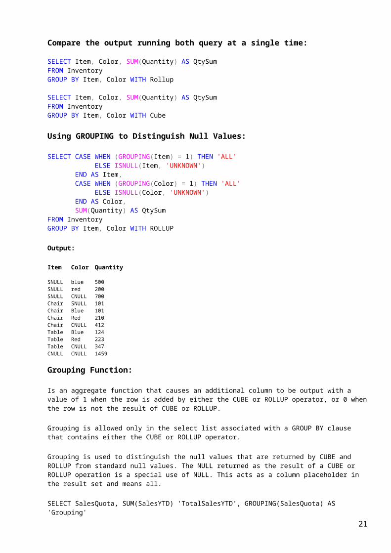
Compare the output running both query at a single time:

SELECT Item, Color, SUM(Quantity) AS QtySumFROM InventoryGROUP BY Item, Color WITH Rollup

SELECT Item, Color, SUM(Quantity) AS QtySumFROM InventoryGROUP BY Item, Color WITH Cube

Using GROUPING to Distinguish Null Values:

SELECT CASE WHEN (GROUPING(Item) = 1) THEN 'ALL' ELSE ISNULL(Item, 'UNKNOWN') END AS Item, CASE WHEN (GROUPING(Color) = 1) THEN 'ALL' ELSE ISNULL(Color, 'UNKNOWN') END AS Color, SUM(Quantity) AS QtySumFROM InventoryGROUP BY Item, Color WITH ROLLUP

Output:

Item Color Quantity

SNULL blue 500SNULL red 200SNULL CNULL 700Chair SNULL 101Chair Blue 101Chair Red 210Chair CNULL 412Table Blue 124Table Red 223Table CNULL 347CNULL CNULL 1459

Grouping Function:

Is an aggregate function that causes an additional column to be output with a value of 1 when the row is added by either the CUBE or ROLLUP operator, or 0 when the row is not the result of CUBE or ROLLUP.

Grouping is allowed only in the select list associated with a GROUP BY clause that contains either the CUBE or ROLLUP operator.

Grouping is used to distinguish the null values that are returned by CUBE and ROLLUP from standard null values. The NULL returned as the result of a CUBE or ROLLUP operation is a special use of NULL. This acts as a column placeholder in the result set and means all.

SELECT SalesQuota, SUM(SalesYTD) 'TotalSalesYTD', GROUPING(SalesQuota) AS 'Grouping'FROM Sales.SalesPersonGROUP BY SalesQuota WITH ROLLUP

The output looks as following:

SalesQuota TotalSalesYTD Grouping --------- ------------- --------NULL 1533087.5999 0250000.00 33461260.59 0300000.00 9299677.9445 0NULL 44294026.1344 1

17

The above result set shows two null values under SalesQuota. The first NULL represents the group of null values from this column in the table. The second NULL is in the summary row added by the ROLLUP operation. The summary row shows the TotalSalesYTD amounts for all SalesQuota groups and is indicated by 1 in the Grouping column.Set Operators:

Set Operations are used to combine multiple result sets into one single result set. There is BIG difference between “join” and “Combine”. Join is Horizontal operations and “Combine” is vertical operation.

Basically there are 3 set operators available in SQL Server.

Union / Union All: This is to combine two or more result sets into single with / without duplicate.

Except: Takes the data from one result set where there is no matching in another.

Intersect: Takes the data from both the result sets which are in common.

Rules on Set Operations:

The column names or aliases must be determined by the first select. Every select must have the same number of columns, and each lineup of

columns must share the same data-type family. Expressions may be added to the select statements to identify the source of

the row so long as the column is added to every select.

select * , 'Old_DEPT' as NF from HumanResources.departmentunion all

select * , 'New_DEPT' as NF from HumanResources.Dept ORDER BY clause should be part of the last statement, which orders the

results. GROUP BY and HAVING clauses can be used only within individual queries;

they cannot be used to affect the final result set. UNION, EXCEPT and INTERSECT can be used within an INSERT statement.

Union & Union All:

Union and Union All combine the results of two or more queries into a single result set that includes all the rows that belong to all queries in the union. UNION operator eliminates the duplicate records meaning that if the same record is in both the tables then it will pickup the record from only one table.

When you use UNION ALL operator it will not eliminate the duplicate records. If you have the same record in both tables then in the final output you will see both the records.

Create tow table Employee and Employee_HIST for set operators practice:

create table Employee(EmployeeID char(5),FName varchar(20),Salary int,DOJ datetime)

Insetr the following data in Employ table:EmployeeID FName Salary DOJE001 Ram 30000 2007-04-15E002 Rabi 20000 2008-04-15E002 Rabi 20000 2008-04-15 E003 Rajwant 25000 2008-09-15 E004 Kuldeep 28000 2009-09-11 E004 Kuldeep 28000 2009-09-11

18

Insetr the following data in Employ_HIST table:

EmployeeID FName Salary DOJE0010 Hari 29000 2005-09-11E0010 Hari 29000 2005-09-11E0011 Ajay 24000 2009-01-01E0011 Ajay 24000 2009-01-01E001 Ram 30000 2007-04-15E002 Rabi 20000 2008-04-15E002 Rabi 20000 2008-04-15E003 Rajwant 25000 2008-09-15E004 Kuldeep 28000 2009-09-11E004 Kuldeep 28000 2009-09-11

Example of Union:

SELECT EmployeeID,FName,Salary,DOJ from EmployeeUNIONSELECT EmployeeID,FName,Salary,DOJ from Employee_HIST

Output:EmployeeID FName Salary DOJE001 Ram 30000 2007-04-15 00:00:00.000E0010 Hari 29000 2005-09-11 00:00:00.000E0011 Ajay 24000 2009-01-01 00:00:00.000E002 Rabi 20000 2008-04-15 00:00:00.000E003 Rajwant 25000 2008-09-15 00:00:00.000E004 Kuldeep 28000 2009-09-11 00:00:00.000Example of Union All:

SELECT EmployeeID,FName,Salary,DOJ from EmployeeUNION AllSELECT EmployeeID,FName,Salary,DOJ from Employee_HIST

Output:EmployeeID FName Salary DOJE001 Ram 30000 2007-04-15 00:00:00.000E002 Rabi 20000 2008-04-15 00:00:00.000E002 Rabi 20000 2008-04-15 00:00:00.000E003 Rajwant 25000 2008-09-15 00:00:00.000E004 Kuldeep 28000 2009-09-11 00:00:00.000E004 Kuldeep 28000 2009-09-11 00:00:00.000E0010 Hari 29000 2005-09-11 00:00:00.000E0010 Hari 29000 2005-09-11 00:00:00.000E0011 Ajay 24000 2009-01-01 00:00:00.000E0011 Ajay 24000 2009-01-01 00:00:00.000E001 Ram 30000 2007-04-15 00:00:00.000E002 Rabi 20000 2008-04-15 00:00:00.000E002 Rabi 20000 2008-04-15 00:00:00.000E003 Rajwant 25000 2008-09-15 00:00:00.000E004 Kuldeep 28000 2009-09-11 00:00:00.000E004 Kuldeep 28000 2009-09-11 00:00:00.000

Intersection:

This operator is used to combine multiple result sets into single to fetch the common records in multiple result sets. Inner join finds common rows horizontally, while an intersect finds common rows vertically.

When you use intersect operator it will give you the common records but unique from both the tables meaning the same records that are available in both the tables.

SELECT EmployeeID,FName,Salary,DOJ from Employee

19

INTERSECT SELECT EmployeeID,FName,Salary,DOJ from Employee_HIST

Output:EmployeeID FName Salary DOJE001 Ram 30000 2007-04-15 00:00:00.000E002 Rabi 20000 2008-04-15 00:00:00.000E003 Rajwant 25000 2008-09-15 00:00:00.000E004 Kuldeep 28000 2009-09-11 00:00:00.000

Except:

This is used to return any distinct rows from the left query (table Used: Employee_HIST) that is not found on the right query (table Used: Employee).

The following example fetches only the records which are in Employee_HIST but not in Employee.

SELECT EmployeeID,FName,Salary,DOJ from Employee_HISTexcept SELECT EmployeeID,FName,Salary,DOJ from Employee

Output:EmployeeID FName Salary DOJ

E0010 Hari 29000 2005-09-11 00:00:00.000E0011 Ajay 24000 2009-01-01 00:00:00.000

The above records are available only in Employee_HIST table. It these records are also added in Employee table and run the above query, the output would be zero records. If the position of the above query is changed without adding the above records in Employee table,again it gives zero record output

Case Statements:

All programming languages use conditional statements. Such statements are of two types:

IF….THEN….Else….END IF Case Expressions

SQL is not an exception. Procedural SQL or PL (SQL programming) uses both of the above conditional processing constructs. But simply SQL statement does not process with ‘IF….THEN….Else….END IF’. For this purpose, SQL uses Case statements. It is equivalent to IIF statement in MS Access. CASE expressions can be used in SQL anywhere an expression can be used.

Example of where CASE expressions can be used include in the SELECT list, WHERE clauses, HAVING clauses, IN lists, DELETE and UPDATE statements, and inside of built-in functions.

Case statement has to forms. Simple Case Expression Searched Case Expression

The SQL Case statement has WHEN, THEN AND ELSE clauses along with END terminator.

General Syntax of Case Statements:

CASE [expression] WHEN [value | Boolean expression] THEN Return Value

ELSE Return ValueEND

Simple Case Expression / statement:

20

A simple CASE expression checks one expression against multiple values. Within a SELECT statement, a simple CASE expression allows only an equality check; no other comparisons are made. A simple CASE expression operates by comparing the first expression to the expression in each WHEN clause for equivalency. If these expressions are equivalent, the expression in the THEN clause will be returned.In simple Case Expression, the actual value contains in the Case expression. The value is checked in When clause which we provide without field or variable and any operator.

Syntax:

CASE expression WHEN value1 THEN result1 WHEN value2 THEN result2

………….. WHEN valueN THEN resultN [ ELSE elseResult ]END

Example:

SELECT ProductNumber, ProductLine,Category = CASE ProductLine WHEN 'R' THEN 'Road' WHEN 'M' THEN 'Mountain' WHEN 'T' THEN 'Touring' WHEN 'S' THEN 'Other sale items' ELSE 'Not for sale' END, NameFROM Production.ProductORDER BY ProductNumber

ORSELECT ProductNumber, CASE ProductLine WHEN 'R' THEN 'Road' WHEN 'M' THEN 'Mountain' WHEN 'T' THEN 'Touring' WHEN 'S' THEN 'Other sale items' ELSE 'Not for sale' END as Category, NameFROM Production.ProductORDER BY ProductNumber

Searched CASE expressions:

A searched CASE expression allows comparison operators, and the use of AND/OR between each Boolean expression. The simple CASE expression checks only for equivalent values and can not contain Boolean expressions.

Syntax:

CASE

WHEN booleanExpression1 THEN result1 WHEN booleanExpression2 THEN result2

21

………….. WHEN booleanExpressionN THEN resultN [ ELSE elseResult ]END

Example:

SELECT ProductNumber, ProductLine, CASE WHEN ProductLine = 'R' THEN 'Road' WHEN ProductLine = 'M' THEN 'Mountain' WHEN ProductLine = 'T' THEN 'Touring' WHEN ProductLine = 'S' THEN 'Other sale items' ELSE 'Not for sale' END as Category, Name as PNameFROM Production.ProductORDER BY ProductNumber

Next Example:

SELECT ProductNumber, Name, 'Price Range' = CASE WHEN ListPrice = 0 THEN 'Mfg item - not for resale' WHEN ListPrice < 50 THEN 'Under $50' WHEN ListPrice >= 50 and ListPrice < 250 THEN 'Under $250' WHEN ListPrice >= 250 and ListPrice < 1000 THEN 'Under $1000' ELSE 'Over $1000' ENDFROM Production.ProductORDER BY ProductNumber

Next Example:

SELECT o.CustomerID, SUM(UnitPrice * OrderQty) AS TotalSales,

CASE WHEN SUM(UnitPrice * OrderQty) BETWEEN 0 AND 5000 THEN 'Micro' WHEN SUM(UnitPrice * OrderQty) BETWEEN 5001 AND 10000 THEN 'Small' WHEN SUM(UnitPrice * OrderQty) BETWEEN 10001 AND 15000 THEN 'Medium' WHEN SUM(UnitPrice * OrderQty) BETWEEN 15001 AND 20000 THEN 'Large' WHEN SUM(UnitPrice * OrderQty) > 20000 THEN 'Very Large' END AS OrderGroup

FROM Sales.SalesOrderDetail AS od INNER JOIN Sales.SalesOrderHeader AS o ON od.SalesOrderId = o.SalesOrderId GROUP BY o.CustomerID

Note: Case statement can be used in select, update, delete statements and clauses like IN, WHERE, ORDER BY AND HAVING.

How to sort data conditionally?

First see the output of this query:

22

All branches will be in ascending order and quantity of every branch will be in descending order.

select Date,Branch,PartyName,Item,Itemgroup,QTY,Rate,Value,Vat,BillAmtfrom dbo.PDataorder by branch asc,qty desc

Using Case statement in Order by clause for conditional Sort:

Search Case:This query does not sort on branch rather it finds the specified value in branch and orders on quantity based on descending or ascending order.

select Date,Branch,PartyName,Item,Itemgroup,QTY,Rate,Value,Vat,BillAmtfrom Pdataorder by

Case When Branch = 'Ghaziabad' Then qty end desc ,Case When Branch = 'Gurgaon' Then qty end asc

ORSimple Case

select Date,Branch,PartyName,Item,Itemgroup,QTY,Rate,Value,Vat,BillAmtfrom Pdataorder by

Case Branch When 'Ghaziabad' Then qty end desc ,Case Branch When 'Gurgaon' Then qty end asc

ORselect Date,Branch,PartyName,Item,Itemgroup,QTY,Rate,Value,Vat,BillAmtfrom Pdataorder by

Case When Branch = 'Ghaziabad' Then qty end desc ,Case When Branch = 'Sriniwas Puri' Then qty end desc

Note: Nested Case Statement will not work in Order By.

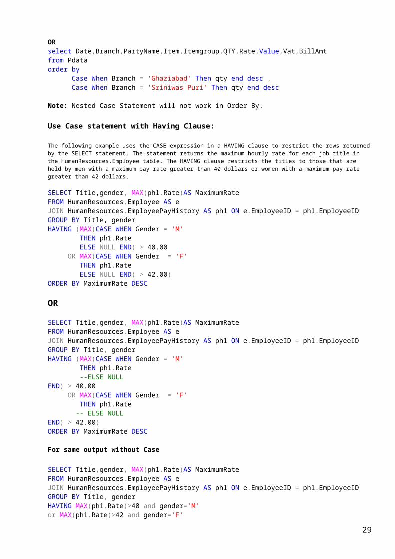
Use Case statement with Having Clause:

The following example uses the CASE expression in a HAVING clause to restrict the rows returned by the SELECT statement. The statement returns the maximum hourly rate for each job title in the HumanResources.Employee table. The HAVING clause restricts the titles to those that are held by men with a maximum pay rate greater than 40 dollars or women with a maximum pay rate greater than 42 dollars.

SELECT Title,gender, MAX(ph1.Rate)AS MaximumRateFROM HumanResources.Employee AS eJOIN HumanResources.EmployeePayHistory AS ph1 ON e.EmployeeID = ph1.EmployeeIDGROUP BY Title, genderHAVING (MAX(CASE WHEN Gender = 'M' THEN ph1.Rate ELSE NULL END) > 40.00 OR MAX(CASE WHEN Gender = 'F' THEN ph1.Rate ELSE NULL END) > 42.00)ORDER BY MaximumRate DESC

OR

SELECT Title,gender, MAX(ph1.Rate)AS MaximumRateFROM HumanResources.Employee AS eJOIN HumanResources.EmployeePayHistory AS ph1 ON e.EmployeeID = ph1.EmployeeIDGROUP BY Title, genderHAVING (MAX(CASE WHEN Gender = 'M'

23

THEN ph1.Rate --ELSE NULL END) > 40.00 OR MAX(CASE WHEN Gender = 'F' THEN ph1.Rate -- ELSE NULL END) > 42.00)ORDER BY MaximumRate DESC

For same output without Case

SELECT Title,gender, MAX(ph1.Rate)AS MaximumRateFROM HumanResources.Employee AS eJOIN HumanResources.EmployeePayHistory AS ph1 ON e.EmployeeID = ph1.EmployeeIDGROUP BY Title, genderHAVING MAX(ph1.Rate)>40 and gender='M'or MAX(ph1.Rate)>42 and gender='F'ORDER BY MaximumRate DESC

*******************************To be covered*************************Using CASE in a SET statement: (Don’t be upset with the following example, we will do it later)

The following example uses the CASE expression in a SET statement in the table-valued function dbo.GetContactInfo. In the AdventureWorks database, all data related to people is stored in the Person.Contact table. For example, the person may be an employee, vendor representative, retail store representative, or a consumer. The function returns the first and last name of a given ContactID and the contact type for that person.The CASE expression in the SET statement determines the value to display for the column ContactType based on the existence of the ContactID column in the Employee, StoreContact, VendorContact, or Individual (consumer) tables.

CREATE FUNCTION dbo.GetContactInformation(@ContactID int)RETURNS @retContactInformation TABLE (

ContactID int NOT NULL,FirstName nvarchar(50) NULL,LastName nvarchar(50) NULL,ContactType nvarchar(50) NULL,

PRIMARY KEY CLUSTERED (ContactID ASC)) AS -- Returns the first name, last name and contact type for the specified contact.BEGIN DECLARE @FirstName nvarchar(50), @LastName nvarchar(50), @ContactType nvarchar(50);

-- Get common contact information SELECT @ContactID = ContactID, @FirstName = FirstName, @LastName = LastName FROM Person.Contact WHERE ContactID = @ContactID;

SET @ContactType = CASE -- Check for employee WHEN EXISTS(SELECT * FROM HumanResources.Employee AS e WHERE e.ContactID = @ContactID) THEN 'Employee'

-- Check for vendor WHEN EXISTS(SELECT * FROM Purchasing.VendorContact AS vc

24

INNER JOIN Person.ContactType AS ct ON vc.ContactTypeID = ct.ContactTypeID WHERE vc.ContactID = @ContactID) THEN 'Vendor Contact'

-- Check for store WHEN EXISTS(SELECT * FROM Sales.StoreContact AS sc INNER JOIN Person.ContactType AS ct ON sc.ContactTypeID = ct.ContactTypeID WHERE sc.ContactID = @ContactID) THEN 'Store Contact'

-- Check for individual consumer WHEN EXISTS(SELECT * FROM Sales.Individual AS i WHERE i.ContactID = @ContactID) THEN 'Consumer' END;

-- Return the information to the caller IF @ContactID IS NOT NULL BEGIN INSERT @retContactInformation SELECT @ContactID, @FirstName, @LastName, @ContactType; END;

RETURN;END;GOSELECT ContactID, FirstName, LastName, ContactTypeFROM dbo.GetContactInformation(2200);GOSELECT ContactID, FirstName, LastName, ContactTypeFROM dbo.GetContactInformation(5);*************************************************************

Operator:An operator is a symbol specifying an action that is performed on one or more expressions. These are the operator categories that SQL Server 2005 uses.

Arithmetic Operators Logical Operators Assignment Operator String Concatenation Operator Comparison Operators

Arithmetic Operators:Arithmetic operators perform mathematical operations on two expressions of one or more of the data types of the numeric data type category.

+ (Addition) - (Subtraction) * (Multiplication) / (Division) % (Modulo): Returns the integer remainder of a division. For example, 12 % 5 = 2 because the remainder of 12 divided by 5 is 2.

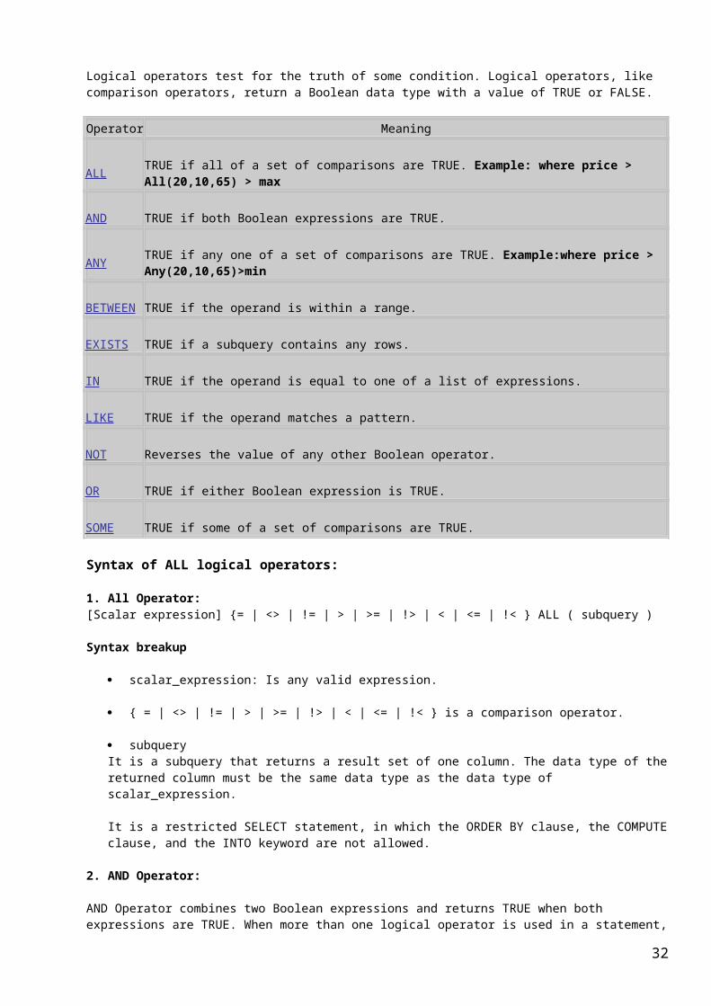
Logical Operators:

Logical operators test for the truth of some condition. Logical operators, like comparison operators, return a Boolean data type with a value of TRUE or FALSE.

Operator Meaning

25

ALL TRUE if all of a set of comparisons are TRUE. Example: where price > All(20,10,65) > max

AND TRUE if both Boolean expressions are TRUE.

ANY TRUE if any one of a set of comparisons are TRUE. Example:where price > Any(20,10,65)>min

BETWEEN TRUE if the operand is within a range.

EXISTS TRUE if a subquery contains any rows.

IN TRUE if the operand is equal to one of a list of expressions.

LIKE TRUE if the operand matches a pattern.

NOT Reverses the value of any other Boolean operator.

OR TRUE if either Boolean expression is TRUE.

SOME TRUE if some of a set of comparisons are TRUE.

Syntax of ALL logical operators:

1. All Operator:[Scalar expression] {= | <> | != | > | >= | !> | < | <= | !< } ALL ( subquery )

Syntax breakup

scalar_expression: Is any valid expression.

{ = | <> | != | > | >= | !> | < | <= | !< } is a comparison operator.

subqueryIt is a subquery that returns a result set of one column. The data type of the returned column must be the same data type as the data type of scalar_expression.

It is a restricted SELECT statement, in which the ORDER BY clause, the COMPUTE clause, and the INTO keyword are not allowed.

2. AND Operator:

AND Operator combines two Boolean expressions and returns TRUE when both expressions are TRUE. When more than one logical operator is used in a statement, the AND operators are evaluated first. You can change the order of evaluation by using parentheses.

Syntax: boolean_expression AND boolean_expression

Here boolean_expression means any expression with comparison operator that returns either True or False

ExampleWhere price > 5 AND Length <= 5 (> , <= are comparison operators, AND is a logical operator)

26

And returns true result if obth expressions return true and false if any one of them returns false.

For example, this query returns only the one row in which the customer ID starts with the number 1 and the store name begins with Bicycle:

SELECT CustomerID, Name FROM AdventureWorks.Sales.StoreWHERE CustomerID LIKE '1%' AND Name LIKE N'Bicycle%'

3. ANY / Some:

This operator compares a scalar value with a single-column set of values.

Syntax:scalar_expression { = | < > | ! = | > | > = | ! > | < | < = | ! < } { ANY } ( subquery )ANY operator returns TRUE when the comparison specified is TRUE for ANY pair (scalar_expression, x) where x is a value in the single-column set; otherwise, returns FALSE.

SELECT NameFROM Production.ProductWHERE ProductSubcategoryID =ANY(SELECT ProductSubcategoryID FROM Production.ProductSubcategory WHERE Name = 'Wheels')

4. BETWEEN:

This operator specifies a range to test.

Syntax: test_expression BETWEEN begin_expression AND end_expression

Here are three expressions in the syntax.

test_expression: Is the expression to test for in the range defined by begin_expression and end_expression. test_expression must be the same data type as both begin_expression and end_expression.

begin_expression: Is any valid expression. begin_expression must be the same data type as both test_expression and end_expression.

end_expression: Is any valid expression. end_expression must be the same data type as both test_expression and begin_expression.

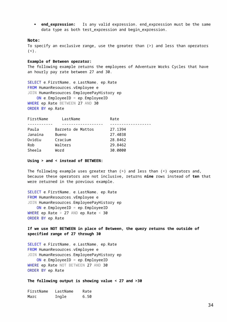
Note:To specify an exclusive range, use the greater than (>) and less than operators (<).

Example of Between operator:The following example returns the employees of Adventure Works Cycles that have an hourly pay rate between 27 and 30.

SELECT e.FirstName, e.LastName, ep.RateFROM HumanResources.vEmployee e JOIN HumanResources.EmployeePayHistory ep ON e.EmployeeID = ep.EmployeeIDWHERE ep.Rate BETWEEN 27 AND 30ORDER BY ep.Rate

FirstName LastName Rate----------- ------------------ ------------------Paula Barreto de Mattos 27.1394Janaina Bueno 27.4038Ovidiu Cracium 28.8462

27

Rob Walters 29.8462Sheela Word 30.0000

Using > and < instead of BETWEEN:

The following example uses greater than (>) and less than (<) operators and, because these operators are not inclusive, returns nine rows instead of ten that were returned in the previous example.

SELECT e.FirstName, e.LastName, ep.RateFROM HumanResources.vEmployee e JOIN HumanResources.EmployeePayHistory ep ON e.EmployeeID = ep.EmployeeIDWHERE ep.Rate > 27 AND ep.Rate < 30ORDER BY ep.Rate

If we use NOT BETWEEN in place of Between, the query returns the outside of specified range of 27 through 30

SELECT e.FirstName, e.LastName, ep.RateFROM HumanResources.vEmployee e JOIN HumanResources.EmployeePayHistory ep ON e.EmployeeID = ep.EmployeeIDWHERE ep.Rate NOT BETWEEN 27 AND 30ORDER BY ep.Rate

The following output is showing value < 27 and >30

FirstName LastName RateMarc Ingle 6.50Reed Koch 6.50Laura Norman 60.0962Terri Duffy 63.4615Brian Welcker 72.1154

5. EXISTS

This operator specifies a subquery to test for the existence of rows.

Syntax: EXISTS subqueryNote: This seems illogical but should be used for logical and relevant output.

See how this is illogical:

SELECT DepartmentID, Name FROM HumanResources.Department WHERE EXISTS (select * from Person.ContactType)ORDER BY Name ASC

If subquery returns any row, the outer query gives output where as there is not any logical relation between both queries.But it subquery returns no rows, the outer query also returns no rows.

Here EXISTS operaor symply checks whrther the inner query returns any row or not. If inner query returns any row, that is true value for EXISTS operator and if EXISTS returns true tnen outer query also returns value if source contains information.

6. IN:

This operator determines whether a specified value matches any value in a subquery or a list. If matches, it returns true for Query.

SELECT FirstName, LastName, e.Title

28

FROM HumanResources.Employee AS e JOIN Person.Contact AS c ON e.ContactID = c.ContactIDWHERE e.Title IN ('Design Engineer', 'Tool Designer', 'Marketing Assistant')

Note: IN operator may contain specified list of values or a subquery of single column with multiple values.

7. Like:

This operator determines whether a specific character string matches a specified pattern. A pattern can include regular characters and wildcard characters. During pattern matching, regular characters must exactly match the characters specified in the character string. However, wildcard characters can be matched with arbitrary fragments of the character string. Using wildcard characters makes the LIKE operator more flexible than using the = and != string comparison operators. If any one of the arguments are not of character string data type, the SQL Server 2005 Database Engine converts them to character string data type, if it is possible.

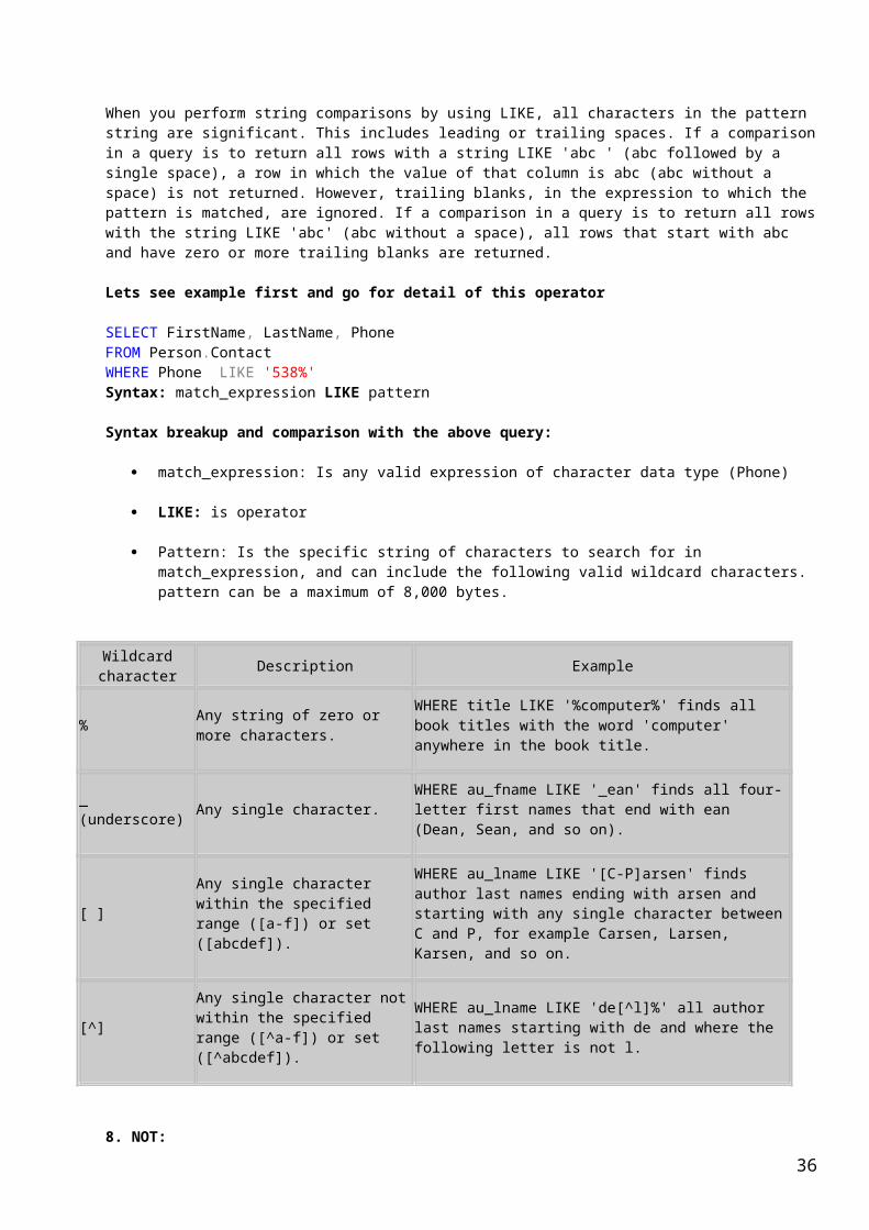
When you perform string comparisons by using LIKE, all characters in the pattern string are significant. This includes leading or trailing spaces. If a comparison in a query is to return all rows with a string LIKE 'abc ' (abc followed by a single space), a row in which the value of that column is abc (abc without a space) is not returned. However, trailing blanks, in the expression to which the pattern is matched, are ignored. If a comparison in a query is to return all rows with the string LIKE 'abc' (abc without a space), all rows that start with abc and have zero or more trailing blanks are returned.

Lets see example first and go for detail of this operator

SELECT FirstName, LastName, PhoneFROM Person.ContactWHERE Phone LIKE '538%'Syntax: match_expression LIKE pattern

Syntax breakup and comparison with the above query:

match_expression: Is any valid expression of character data type (Phone)

LIKE: is operator

Pattern: Is the specific string of characters to search for in match_expression, and can include the following valid wildcard characters. pattern can be a maximum of 8,000 bytes.

Wildcard character

Description Example

%Any string of zero or more characters.

WHERE title LIKE '%computer%' finds all book titles with the word 'computer' anywhere in the book title.

_ (underscore) Any single character.

WHERE au_fname LIKE '_ean' finds all four-letter first names that end with ean (Dean, Sean, and so on).

[ ] Any single character within the specified range ([a-f]) or set ([abcdef]).

WHERE au_lname LIKE '[C-P]arsen' finds author last names ending with arsen and starting with any single character between C and P, for example Carsen, Larsen,

29

Karsen, and so on.

[^]

Any single character not within the specified range ([^a-f]) or set ([^abcdef]).

WHERE au_lname LIKE 'de[^l]%' all author last names starting with de and where the following letter is not l.

8. NOT: Negates the Boolean expression specified by the predicate.

Syntax:[NOT] boolean_expression

boolean_expression means any expression that comes with logical operators and returns either TRUE or False

The NOT operator reverses the value of any Boolean expression. i.e. if TRUE comes with NOT tnen NOT + TRUE = FALSEIf FALSE comes with NOT tnen NOT + FALSE = TRUE

The following example finds all Silver colored bicycles that do not have a standard price over $400.

SELECT ProductID, Name, Color, ProductNumber,StandardCostFROM Production.ProductWHERE ProductNumber LIKE 'BK-%' AND Color = 'Silver' AND NOT StandardCost > 400

PRODID Name Color ProductNumber StandardCost984 Mountain-500 Silver,40 Silver BK-M18S-40 308.2179985 Mountain-500 Silver,42 Silver BK-M18S-42 308.2179986 Mountain-500 Silver,44 Silver BK-M18S-44 308.2179987 Mountain-500 Silver,48 Silver BK-M18S-48 308.2179988 Mountain-500 Silver,52 Silver BK-M18S-52 308.2179

Just remove NOT operator and see the result:

SELECT ProductID, Name, Color, ProductNumber,StandardCostFROM Production.ProductWHERE ProductNumber LIKE 'BK-%' AND Color = 'Silver' AND StandardCost > 400

PRODID Name Color ProductNumber StandardCost771 Mountain-100 Silver, 38 Silver BK-M82S-38 1912.1544772 Mountain-100 Silver, 42 Silver BK-M82S-42 1912.1544773 Mountain-100 Silver, 44 Silver BK-M82S-44 1912.1544774 Mountain-100 Silver, 48 Silver BK-M82S-48 1912.1544779 Mountain-200 Silver, 38 Silver BK-M68S-38 1265.6195780 Mountain-200 Silver, 42 Silver BK-M68S-42 1265.6195781 Mountain-200 Silver, 46 Silver BK-M68S-46 1265.6195

8. OR:

This operator connects two conditions like AND operator, but it returns TRUE when either of the conditions is true. When more than one logical operator is used in a statement, OR operators are evaluated after AND operators. However, you can change the order of evaluation by using parentheses.

Syntax: boolean_expression OR boolean_expression

boolean_expression ss any valid expression that returns TRUE, FALSE, or UNKNOWN.

30

The following query returns the all rows whose customer IDs start with 1 or whose store name begins with Bicycle:

SELECT CustomerID, Name FROM AdventureWorks.Sales.StoreWHERE CustomerID LIKE '1%' OR Name LIKE 'Bicycle%'

Assignment Operator:

The equal sign (=) is the only Transact-SQL assignment operator. This operator is used to assign any value to a variable or a column heading of a select statement.

Example of Assignment Operator:

select FName ='Rabi', LName = 'Puri', Address = 'I - 259,Gali No-8,Jaitpur'Output:FName LName AddressRabi Puri I - 259,Gali No-8,Jaitpur

If you use the same operator to compare value of a variable or a column, it is comparison operator.

SELECT FirstName, LastNameFROM Person.Contactwhere LastName = 'Adams'

Comparison Operators:

Comparison operators test whether two expressions are the same. Comparison operators can be used on all expressions except expressions of the text, ntext, or image data types. The following table lists the Transact-SQL comparison operators.

Operator Meaning

= (Equals) Equal to

> (Greater Than) Greater than

< (Less Than) Less than

>= (Greater Than or Equal To) Greater than or equal to

<= (Less Than or Equal To) Less than or equal to

<> (Not Equal To) Not equal to

!= (Not Equal To) Not equal to (not in SQL-92 standard)

!< (Not Less Than) Not less than (not SQL-92 standard)

!> (Not Greater Than) Not greater than (not SQL-92 standard)

DECLARE @MyProduct int;SET @MyProduct = 750; --Assignment operatorIF (@MyProduct <> 0) --Comparison operator

31

SELECT ProductID, Name, ProductNumber FROM Production.Product WHERE ProductID = @MyProduct

String Concatenation Operator:

The plus sign (+) is the string concatenation operator that enables string concatenation.

Example:

select Title +' '+ FirstName +' '+ MiddleName+' '+lastname as FullNamefrom Person.Contact

Subquery:

A subquery is a query that is nested inside a select, insert, update or a delete statement or inside another subquery. A subquery can be used anywhere an expression / field is allowed.

A subquery is also called an inner query or inner select, while the statement containing a subquery is also called an outer query or outer select.

In this example a subquery is used as a column expression named MaxUnitPrice in a SELECT statement.

Example:

SELECT Ord.SalesOrderID, Ord.OrderDate, (SELECT MAX(OrdDet.UnitPrice) FROM Sales.SalesOrderDetail AS OrdDet WHERE Ord.SalesOrderID = OrdDet.SalesOrderID) AS MaxUnitPriceFROM Sales.SalesOrderHeader AS Ord

Subqueries can be alternatively used in place of joins. However, in some cases where existence must be checked, a join yields better performance. Otherwise, the nested query must be processed for each result of the outer query to ensure elimination of duplicates. In such cases, a join approach would yield better results. The following is an example showing both a subquery SELECT and a join SELECT that return the same result set:

--SELECT statement built using a subquery. SELECT NameFROM Production.ProductWHERE ListPrice = (SELECT ListPrice FROM Production.Product WHERE Name = 'Chainring Bolts' )

--SELECT statement built using a join that returns the same result set.

SELECT Prd1. NameFROM Production.Product AS Prd1 JOIN Production.Product AS Prd2 ON (Prd1.ListPrice = Prd2.ListPrice)WHERE Prd2. Name = 'Chainring Bolts' A subquery nested in the outer SELECT statement has the following components:

A regular SELECT query including the regular select list components. A regular FROM clause including one or more table or view names. An optional WHERE clause.

32

An optional GROUP BY clause. An optional HAVING clause.

The SELECT query of a subquery is always enclosed in parentheses. It cannot include a COMPUTE , and may only include an ORDER BY clause when a TOP clause is also specified.( The ORDER BY clause is invalid in views, inline functions, derived tables, subqueries, and common table expressions, unless TOP or FOR XML is also specified.)

A subquery can be nested inside the WHERE or HAVING clause of an outer SELECT, INSERT, UPDATE, or DELETE statement, or inside another subquery. Up to 32 levels of nesting is possible, although the limit varies based on available memory and the complexity of other expressions in the query. Individual queries may not support nesting up to 32 levels. A subquery can appear anywhere as an expression can be used.

Note: If a table appears only in a subquery and not in the outer query, then columns from that table cannot be included in the output (the select list of the outer query. For this, either you use a correlated subquery or join).

Statements that include a subquery usually take one of these formats: WHERE expression [NOT] IN (subquery)->List operator WHERE expression comparison_operator [ANY | ALL] (subquery)-> Modified

comparison_operator WHERE [NOT] EXISTS (subquery)->Boolean Operator WHERE expression comparison_operator (subqyery)-> comparison_operator

There are three basic types of subqueries.

1. A subquery that Operates on lists introduced with IN, or those that a comparison operator modified by ANY or ALL (modified comparison operator).(Subquery that returens multiple value)!<, !>, !=, >, <, <=, >=,= are Comparision operators.If these operators are followed by ANY or ALL like >ANY(5,7,10) are called modified comparison operators.

2. A subquery with an unmodified comparison operator and must return a single value.(Subquery that returns single value)

3. A subquery that checks the existence of data in other table with EXISTS operator.(Subquery that checks existance of rows in other table and returns true or false)

Rules of subquery:

The select list of a subquery introduced with a comparison operator can include only one expression or column name single value(except that EXISTS and IN operate on SELECT * or a list, respectively).

If the WHERE clause of an outer query includes a column name, it must be join-compatible with the column in the subquery select list.

The ntext, text, and image data types cannot be used in the select list of subqueries.

Because they must return a single value, subqueries introduced by an unmodified comparison operator (one not followed by the keyword ANY or ALL) cannot include GROUP BY and HAVING clauses. If you need to use group by and having clause in subquery, you have to go one step ahead to produce a single colume having single value filtering the group with having clause and convert the subquery into derived table and select the single column with middle sub query.

SELECT NameFROM Production.ProductWHERE ListPrice =

(select ListPrice from (SELECT Name, sum(ListPrice) as ListPrice

33

FROM Production.Product group by Name

having Name = 'Chainring Bolts' ) aaa)order by name desc

The DISTINCT keyword cannot be used with subqueries that include GROUP BY. The COMPUTE and INTO clauses cannot be specified. ORDER BY can only be specified when TOP is also specified.

Note: The select list of a subquery introduced with EXISTS, by convention, has an asterisk (*) instead of a single column name. The rules for a subquery introduced with EXISTS are the same as those for a standard select list, because a subquery introduced with EXISTS creates an existence test and returns TRUE or FALSE, instead of data.

Types of subquery in detail with examples:

1. A subquery that Operates on lists introduced with IN, or those that a comparison operator modified by ANY or ALL.

Subqueries with IN [NOT IN]:The result of a subquery introduced with IN (or with NOT IN) is a list of zero or more values. After the subquery returns results, the outer query makes use of them.

Example:The following query finds the names of all the wheel products that Adventure Works Cycles makes.

SELECT NameFROM Production.ProductWHERE ProductSubcategoryID IN (SELECT ProductSubcategoryID FROM Production.ProductSubcategory WHERE Name = 'Wheels' or Name ='Cleaners')

Output:LL Mountain Front WheelML Mountain Front WheelHL Mountain Front WheelLL Road Front WheelML Road Front WheelHL Road Front Wheel…………………….

NOT IN:

SELECT NameFROM Production.ProductWHERE ProductSubcategoryID NOT IN (SELECT ProductSubcategoryID FROM Production.ProductSubcategory WHERE Name = 'Wheels' or Name ='Cleaners')

HL Road Frame - Black, 58HL Road Frame - Red, 58Sport-100 Helmet, RedSport-100 Helmet, BlackMountain Bike Socks, MMountain Bike Socks, LSport-100 Helmet, BlueAWC Logo Cap

34

Long-Sleeve Logo Jersey, S………………………………………

One difference in using a join rather than a subquery for this and similar problems is that the join lets you show columns from more than one table in the result. For example, if you want to include the name of the product subcategory in the result, you must use a join version.

SELECT p.Name as productName, s.Name as CategoryNameFROM Production.Product pINNER JOIN Production.ProductSubcategory sON p.ProductSubcategoryID = s.ProductSubcategoryIDAND s.Name = 'Wheels'

productName CategoryName

LL Mountain Front Wheel WheelsML Mountain Front Wheel WheelsHL Mountain Front Wheel WheelsLL Road Front Wheel WheelsML Road Front Wheel WheelsHL Road Front Wheel WheelsTouring Front Wheel WheelsLL Mountain Rear Wheel Wheels

Note: Instead of using AND, we can use where clause:SELECT p.Name as productName, s.Name as CategoryNameFROM Production.Product pINNER JOIN Production.ProductSubcategory sON p.ProductSubcategoryID = s.ProductSubcategoryIDwhere s.Name = 'Wheels'

One more example with IN operator

The following query finds the name of all vendors whose credit rating is good, from whom Adventure Works Cycles orders at least 20 items, and whose average lead time to deliver is less than 16 days.

SELECT NameFROM Purchasing.VendorWHERE CreditRating = 1AND VendorID IN (SELECT VendorID FROM Purchasing.ProductVendor WHERE MinOrderQty >= 20 AND AverageLeadTime < 16)

Subquery with modified comparison operators:

Comparison operators that introduce a subquery can be modified by the keywords ALL or ANY. SOME is an SQL-92 standard equivalent for ANY.

Subqueries introduced with a modified comparison operator return a list of zero or more values and can include a GROUP BY or HAVING clause. These subqueries can be restated with EXISTS.

Using the > comparison operator as an example, >ALL means greater than every value. In other words, it means greater than the maximum value. For example, >ALL (1, 2, 3) means greater than 3. >ANY means greater than at least one value, that is, greater than the minimum. So >ANY (1, 2, 3) means greater than 1.

Example:

35

The following query provides an example of a subquery introduced with a comparison operator modified by ANY. It finds the products whose list prices are greater than or equal to the maximum list price of any product subcategory.

First try this query to simply see the listprice:

SELECT Name,ListPriceFROM Production.Productwhere listprice >0order by listpriceThen try this:

SELECT Name,ListPriceFROM Production.ProductWHERE ListPrice >= ANY (SELECT MAX (ListPrice) FROM Production.Product GROUP BY ProductSubcategoryID)

For each Product subcategory, the inner query finds the maximum list price. The outer query looks at all of these values and determines which individual product's list prices are greater than or equal to any product subcategory's maximum list price. If ANY is changed to ALL, the query will return only those products whose list price is greater than or equal to all the list prices returned in the inner query.

If the subquery does not return any values, the entire query fails to return any values.

The =ANY operator is equivalent to IN. For example, to find the names of all the wheel products that Adventure Works Cycles makes, you can use either IN or =ANY.

SELECT NameFROM Production.ProductWHERE ProductSubcategoryID =ANY (SELECT ProductSubcategoryID FROM Production.ProductSubcategory WHERE Name = 'Wheels')

The < >ANY, < >ALL and NOT IN:

The < >ANY operator, however, differs from NOT IN: < >ANY means not = a, or not = b, or not = c. NOT IN means not = a, and not = b, and not = c. <>ALL means the same as NOT IN.

For example, the following query finds customers located in a territory not covered by any sales persons.

SELECT CustomerIDFROM Sales.CustomerWHERE TerritoryID <> ANY (SELECT TerritoryID FROM Sales.SalesPerson)

The results include all customers, except those whose sales territories are NULL, because every territory that is assigned to a customer is covered by a sales person. The inner query finds all the sales territories covered by sales persons, and then, for each territory, the outer query finds the customers who are not in one.

For the same reason, when you use NOT IN in this query, the results include none of the customers.

36

You can get the same results with the < >ALL operator, which is equivalent to NOT IN.

2. A subquery with an comparison (unmodified) operator and must return a single value.

Subqueries can be introduced with one of the comparison operators (=, < >, >, > =, <, ! >, ! <, or < =).

A subquery introduced with an unmodified comparison operator (a comparison operator not followed by ANY or ALL) must return a single value rather than a list of values, like subqueries introduced with IN. If such a subquery returns more than one value, Microsoft SQL Server 2005 displays an error message.

To use a subquery introduced with an unmodified comparison operator, you must be familiar enough with your data and with the nature of the problem to know that the subquery will return exactly one value.

For example, if you assume each sales person only covers one sales territory, and you want to find the customers located in the territory covered by Linda Mitchell, you can write a statement with a subquery introduced with the simple = comparison operator.

SELECT CustomerIDFROM Sales.CustomerWHERE TerritoryID = (SELECT TerritoryID FROM Sales.SalesPerson WHERE SalesPersonID = 276)

If, however, Linda Mitchell covered more than one sales territory, then an error message would result. Instead of the = comparison operator, an IN formulation could be used (= ANY also works).

Subqueries introduced with unmodified comparison operators often include aggregate functions, because these return a single value. For example, the following statement finds the names of all products whose list price is greater than the average list price.

SELECT NameFROM Production.ProductWHERE ListPrice > (SELECT AVG (ListPrice) FROM Production.Product)

Because subqueries introduced with unmodified comparison operators must return a single value, they cannot include GROUP BY or HAVING clauses unless you know the GROUP BY or HAVING clause itself returns a single value. For example, the following query finds the products priced higher than the lowest-priced product that is in subcategory 14.

SELECT NameFROM Production.ProductWHERE ListPrice > (SELECT MIN (ListPrice) FROM Production.Product GROUP BY ProductSubcategoryID HAVING ProductSubcategoryID = 14)If you remove having clause, the subquery returns multiple value due to grouping and returns following error:

Subquery returned more than 1 value. This is not permitted when the subquery follows =, !=, <, <= , >, >= or when the subquery is used as an expression.

37

Try to see error:

SELECT NameFROM Production.ProductWHERE ListPrice > (SELECT MIN (ListPrice) FROM Production.Product GROUP BY ProductSubcategoryID)

3. A subquery that checks the existence of data introduced with EXISTS operator.

This operator specifies a subquery to test for the existence of rows.

Syntax: EXISTS subqueryNote: This seems illogical but should be used for logical and relevant output.

See how this is illogical:

SELECT DepartmentID, Name FROM HumanResources.Department WHERE EXISTS (select * from Person.ContactType)ORDER BY Name ASC

If subquery returns any row, the outer query gives output where as there is not any logical relation between both queries.But it subquery returns no rows, the outer query also returns no rows.

Here EXISTS operaor symply checks whrther the inner query returns any row or not. If inner query returns any row, that is true value for EXISTS operator and if EXISTS returns true tnen outer query also returns value if source contains information.

Comparing queries by using EXISTS and IN

The following example compares two queries that are equivalent. The first query uses EXISTS and the second query uses IN.

SELECT DISTINCT c.FirstName, c.LastName, e.DepartmentIDFROM Person.Contact c JOIN HumanResources.Employee eON e.ContactID = c.ContactID WHERE EXISTS(SELECT *FROM HumanResources.Department dWHERE e.DepartmentID = d.DepartmentIDAND d.Name = 'Purchasing')

The following query uses IN.

SELECT DISTINCT c.FirstName, c.LastName, e.DepartmentIDFROM Person.Contact c JOIN HumanResources.Employee eON e.ContactID = c.ContactID WHERE DepartmentID IN(SELECT DepartmentID FROM HumanResources.Department dWHERE d.Name = 'Purchasing')

Correlated Subquery:

A correlated subquery is a SELECT statement nested inside another SQL statement, which contains a reference to one or more columns in the outer query. In queries that include a correlated subquery (also known as a repeating subquery), the subquery depends on the outer query for its values. This means that the subquery

38

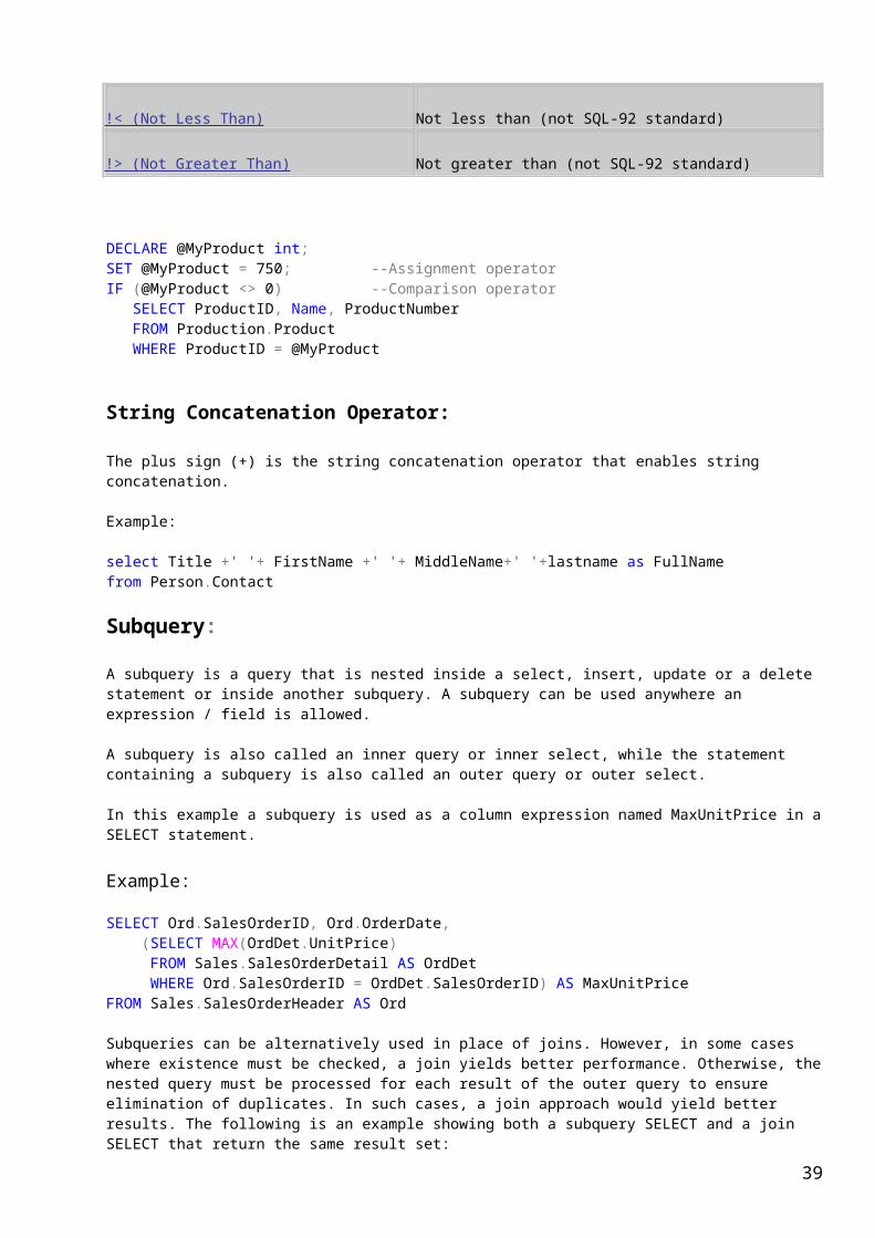
is executed repeatedly, once for each row that might be selected by the outer query.This is the main difference between a correlated subquery and just a plain subquery. A plain subquery is not dependent on the outer query, can be run independently of the outer query, and will return a result set. A correlated subquery, since it is dependent on the outer query will return a syntax errors if it is run by itself.

Steps of execution of correlated subquery:

1. The outer query obtains a record from source and passes it into the inner query.

2. The inner query executes based on the value passed by the outer query.3. The inner query then passes the value from its results back to the outer

query which uses them to finish its processing.

Due to the fact that a correlated sub-query can be executed for every row returned by the outer query, performance can be degraded.

The main advantage of a correlated sub-query is that you can use it to solve problems that cannot be solved with a conventional SQL Server query. Results such as running total sales columns or the highest selling product in each state can easily be accomplished with the use of a correlated sub-query.

Use a correlated subquery with a comparison operator to find out those products where the quantity sold is less than the average quantity for sales of that product.

SELECT ProductID, OrderQtyFROM Sales.SalesOrderDetail s1WHERE s1.OrderQty < (SELECT AVG (s2.OrderQty) FROM Sales.SalesOrderDetail s2 WHERE s2.ProductID = s1.ProductID)

Summary output of above querySELECT ProductID, count(OrderQty)FROM Sales.SalesOrderDetail s1WHERE s1.OrderQty < (SELECT AVG (s2.OrderQty) FROM Sales.SalesOrderDetail s2 WHERE s2.ProductID = s1.ProductID)group by productidorder by ProductID desc

Use a correlated subquery with a comparison operator to find sales where the quantity more than the average quantity for sales of that product.

SELECT ProductID, OrderQtyFROM Sales.SalesOrderDetail s1WHERE s1.OrderQty > (SELECT AVG (s2.OrderQty) FROM Sales.SalesOrderDetail s2 WHERE s2.ProductID = s1.ProductID)

Summary output of above query

SELECT ProductID, count(OrderQty)FROM Sales.SalesOrderDetail s1WHERE s1.OrderQty > (SELECT AVG (s2.OrderQty) FROM Sales.SalesOrderDetail s2 WHERE s2.ProductID = s1.ProductID)group by productid

39

order by ProductID desc

One more example to find all products that have a price greater than the average for products of its subcategory:

SELECT p1.ProductSubcategoryID, p1.NameFROM Production.Product p1WHERE p1.ListPrice > (SELECT AVG (p2.ListPrice) FROM Production.Product p2 WHERE p1.ProductSubcategoryID = p2.ProductSubcategoryID)

Correlated Subqueries in a HAVING Clause:

A correlated subquery can also be used in the HAVING clause of an outer query. The following example finds the product models for which the maximum list price is less than twice the average for the model.

SELECT p1.ProductModelID,count(P1.ListPrice)FROM Production.Product p1GROUP BY p1.ProductModelIDHAVING MAX(p1.ListPrice) < ALL(SELECT 2 * AVG(p2.ListPrice)FROM Production.Product p2WHERE p1.ProductModelID = p2.ProductModelID)

In this case, the subquery is evaluated once for each group defined in the outer query, that is, once for each model of product.

Note:One query for same output in different forms (Join in from clause, join in where clause and correlated subquery)

Join in from clause:

SELECT e.EmployeeIDFROM HumanResources.Employee AS e INNER JOIN Sales.SalesPerson AS s ON e.EmployeeID = s.SalesPersonID

Join in where clause:SELECT e.EmployeeIDFROM HumanResources.Employee AS e, Sales.SalesPerson AS s where e.EmployeeID = s.SalesPersonID

Correlated subquery:

SELECT e.EmployeeIDFROM HumanResources.Employee AS e where e.EmployeeID =(select s.SalesPersonID from Sales.SalesPerson AS s where e.EmployeeID = s.SalesPersonID)

Uasge of List operator ‘IN’ in a correlated Subquery:

The following example uses IN in a correlated, or repeating, subquery. This is a query that depends on the outer query for its values. The query is executed repeatedly, one time for each row that may be selected by the outer query. This query retrieves one instance of the first and last name of each employee for which the bonus in the SalesPerson table is 5000.00 and for which the employee identification numbers match in the Employee and SalesPerson tables.

SELECT DISTINCT c.LastName, c.FirstName FROM Person.Contact c JOIN HumanResources.Employee eON e.ContactID = c.ContactID WHERE 5000.00 IN

40

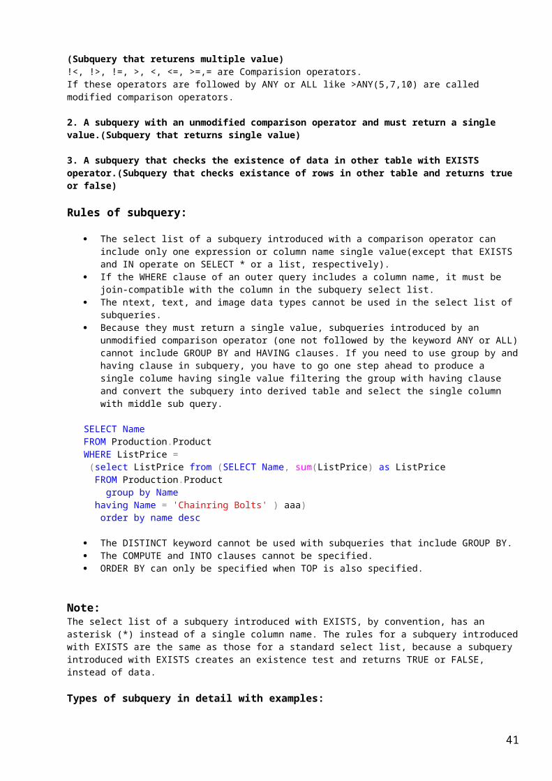
(SELECT BonusFROM Sales.SalesPerson spWHERE e.EmployeeID = sp.SalesPersonID)

Bonus field cannot be used in place of WHERE 5000.00 because this is the field of a table on which correlated subquery is defined and outer query does not identify it.

Look at the example of multiple nested subquery:

SELECT c.LastName, c.FirstName FROM Person.Contact c JOIN HumanResources.Employee eON e.ContactID = c.ContactID WHERE EmployeeID IN

(SELECT SalesPersonID FROM Sales.SalesOrderHeaderWHERE SalesOrderID IN

(SELECT SalesOrderID FROM Sales.SalesOrderDetailWHERE ProductID IN

(SELECT ProductID FROM Production.Product p WHERE ProductNumber in

(select p.ProductNumber from Production.Product p where p.ProductNumber like 'BK%'))))

Inline View and Derived Table:Inline view and derived table are same. A derived table is a select statement inside parenthesis, with an alias, used as a table in a join or union. Derived tables are very common with JOIN clauses because they have a defined name, which is necessary for the join, unlike subqueries. They are an alternative to temporary tables in the same situations as subqueries. Another use for derived tables is in row calculations, particularly when there are excessive aggregate functions and CASE statements. Derived tables exist in memory and can only be referenced by the outer SELECT in which they are created.The inner SELECT produces a derived table and replaces a regular table or view. The key thing to remember when using derived tables is that you must always use an alias

Create two tables in test Database (Emp and Sal)and insert data to run following Query:

Select emp_name,TotSal.AnuualSalaryfrom dbo.Emp ejoin (select s.empId,sum(Sal) AnuualSalary from dbo.sal s

group by s.empId)TotSalon e.empId=TotSal.empId

output

emp_name TotSal.AnuualSalaryABCD1 109000ABCD2 147500ABCD3 91500ABCD4 108000ABCD5 80500ABCD6 70300ABCD7 87388ABCD8 15000ABCD9 15000ABCD10 15000

41

ABCD11 15000

More completed example of derived table

SELECT OG.OrderGroup, COUNT(OG.OrderGroup) AS OrderGroupCount from (SELECT o.CustomerID, SUM(UnitPrice * OrderQty) AS TotalSales, CASE WHEN SUM(UnitPrice * OrderQty) BETWEEN 0 AND 5000 THEN 'Micro' WHEN SUM(UnitPrice * OrderQty) BETWEEN 5001 AND 10000 THEN 'Small' WHEN SUM(UnitPrice * OrderQty) BETWEEN 10001 AND 15000 THEN 'Medium' WHEN SUM(UnitPrice * OrderQty) BETWEEN 15001 AND 20000 THEN 'Large' WHEN SUM(UnitPrice * OrderQty) > 20000 THEN 'Very Large' END AS OrderGroup FROM Sales.SalesOrderDetail AS od INNER JOIN Sales.SalesOrderHeader AS o ON od.SalesOrderId = o.SalesOrderId GROUP BY o.CustomerID ) as ogGROUP BY OG.OrderGroup

Top Aanlysis ("TOP" Clause in SQL Server 2005):The "TOP" clause returns the first n number of rows or percentage of rows thereby limiting the number of resulting rows displayed when we are selecting rows in a table.

Select all records:select * from dbo.Sal

Select heighest 5 salary records:Select top (5)* from dbo.Sal order by sal desc

Select 5 percent of total number of records irrespective of order or salary:Select top (5) percent* from dbo.Sal

The TOP clause also comes with another feature called TIES. If you would Like to include similar criteria together when using TOP clause, then TIES can be used.

For example the following query returns the TOP 5 % of the table.

Select top (5) percent * from dbo.Salorder by empid

Output:EmpID SalDate SalE001 2006-01-01 20000E001 2006-02-01 20000E001 2006-03-04 20000E001 2006-04-04 25000E001 2006-05-05 25000

But we know that there is another row with the same EmpID values.

Now let us include the TIES option in the query. Order by clause is mendatory with TIES

42

Select top (5) percent with ties * from dbo.Salorder by empid desc

EmpID SalDate SalE001 2006-01-01 20000E001 2006-02-01 20000E001 2006-03-04 20000E001 2006-04-04 25000E001 2006-05-05 25000E001 2006-06-05 25000E001 2006-10-07 5000E001 2006-11-07 5000E001 2006-12-08 9000E001 2007-01-08 9000E001 2007-02-08 9000E001 2007-03-11 9000E001 2007-04-11 9000E001 2007-05-12 9000

Select a complete record having the highest salary joining to tables Emp and NewSal (without refrential integrity):

select e.EmpID,Emp_Name,JoinDate,salfrom dbo.emp e join dbo.NewSal son e.empid=s.empidwhere sal = (select min(sal) as third_Sal from dbo.NewSalwhere empid in (select top 3 empid from dbo.NewSalorder by sal desc))

Top clause in DML statements:

In SQL Server 2005, Microsoft enhanced the TOP clause to be used in the DML statements as well. Before 2005, TOP was allowed only in SELECT statements to restrict the output to the number of rows specified by the TOP operator. Now we can apply TOP operator to INSERT, UPDATE or DELETE statements as well.

INSERT INTO dbo.NewEmp SELECT top 5 *FROM dbo.Emp

But in SQL Server 2005, we can use following syntax:

Here paranthesis is must with 5 and fields nameINSERT top (5) INTO dbo.NewEmp (EmpID,Emp_Name,JoinDate)SELECT *FROM dbo.Emp

Or

INSERT top (5) INTO dbo.NewEmp (EmpID,Emp_Name,JoinDate)SELECT EmpID,Emp_Name,JoinDateFROM dbo.Emp

Now we will update first three records.But we cannot use order by clause with update statement.

To update 3 top row having minimum salary with 25000, do the following

UPDATE TOP (3) dbo.Sal SET Sal = 25000where sal in (select min(sal) from dbo.Sal)Above query will update three records in the table. We can also use TOP percent clause. Following is the delete statement which deletes 20 percent records from the table.

43

DELETE TOP (20) PERCENT FROM dbo.newEmp

Or

Delete TOP (3) dbo.Sal where sal in (select min(sal) from dbo.Sal)

Dealing with duplicate records:

There are many ways to get rid of duplicate data in SQL server.Hints:

Distinct Keyword Group by & having clause: having (count) > 1 or having (count) =1 Union operator Use Minimum of Identity column grouping with proposed column Special column “RowGiud” in SQL Server 2005

Distinct Keyword:

First create a table in your Test Database

Create Table myTable(myID int identity(1001,1),name varchar(10), add1 varchar(10),add2 varchar(10))

Insert the following data:

myID name add1 add21 Jacky Room 25 Drig Road2 Jack2 Room 29 Drig Road3 Jacky Room 25 Drig Road4 Rabi Room 2 Nepal5 Rabi Room 2 Nepal6 Rabi Room 2 Nepal7 Ram Room 55 India8 Ram Room 55 India9 Ram Room 55 India10 Kuldeep Room 10 UK11 Kuldeep Room 10 UK

Now use all techniques to select duplicate and unique records and delete duplicate records.

The following query pulls all records as above data.Select * from myTable

Distinct keyword selects non-duplicate records based on the combination of all fields. If a table contains a column with unique values, “Select * from myTable”& “Select distinct * from myTable” will give same output. Because one column contains unique values that makes the records unique.

This query also gives the same output as above.Select distinct * from myTableThis query pulls all rows as above.Select Name,add1,add2 from myTable

This query pulls only unique rows because among selected columns, no column contains unique values.

Select distinct Name,add1,add2 from myTablename add1 add2

44

Jack2 Room 29 Drig RoadJacky Room 25 Drig RoadKuldeep Room 10 UKRabi Room 2 NepalRam Room 55 India

Note: The distinct keyword only selects unique records. But it can neither select duplicate records nor can delete duplicate.

Group by & having clause: having (count) > 1 or having (count) = 1

To select only duplicate records, first we have to decide the combination of fields on which we pull duplicate records.

For example, we are taking all fields except identity column.

Run this query:

SELECT Name,add1,add2, Count(*) as No_Of_RowsFROM myTable GROUP BY Name,add1,add2

It simply summaries the data like this:

name add1 add2 No_Of_RowsJack2 Room 29 Drig Road 1Jacky Room 25 Drig Road 2Kuldeep Room 10 UK 2Rabi Room 2 Nepal 3Ram Room 55 India 3

Now run the following query to select duplicate records:

SELECT Name,add1,add2, Count(*) as No_Of_RowsFROM myTable GROUP BY Name,add1,add2HAVING Count(*) > 1

name add1 add2 No_Of_RowsJacky Room 25 Drig Road 2Kuldeep Room 10 UK 2Rabi Room 2 Nepal 3Ram Room 55 India 3

This query selects only duplicate records excluding purely unique records. Also keep in mind that each set of duplicate records contains one unique record. Now run the following query to select purely unique records:

SELECT Name,add1,add2, Count(*) as No_Of_RowsFROM myTable GROUP BY Name,add1,add2HAVING Count(*) < 2

name add1 add2 No_Of_Rows

Jack2 Room 29 Drig Road 1

Note: This query can select only unique and duplicate records based on the number of duplicate. You cannot delete duplicate records because you will also delete one unique record per group.So never do like this to delete duplicate records:

Delete from aaawhere name in(SELECT Name FROM aaa

45

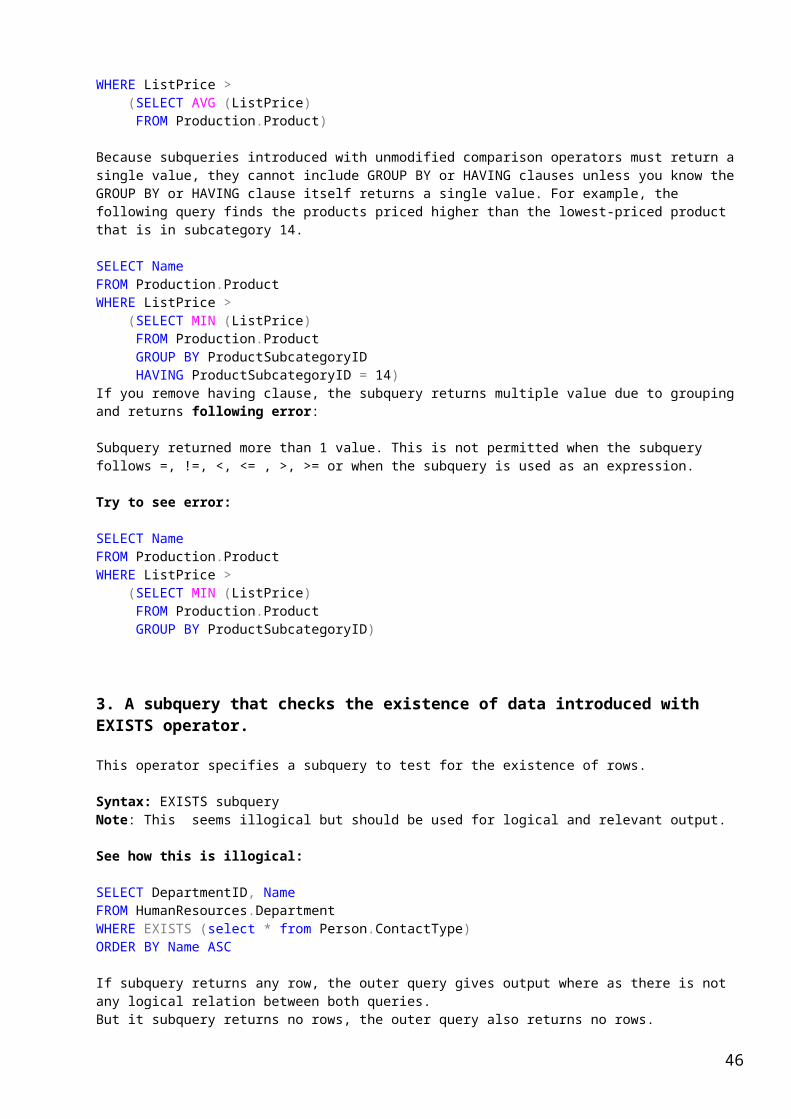
group by nameHAVING Count(*) >1)

Union operator:

Distinct Keyword is used to select unique records from a single source. Union operator is used to select unique records from two or one source. The output of the query with distinct keyword and union operator is same. Both select row based unique records.

Example: for same output

Distinct:select distinct Name,add1,add2 from myTable

Union:select Name,add1,add2 from myTableunionselect Name,add1,add2 from myTable

Use Minimum / Maximum of Identity column grouping with proposed columnIdentity column is long integer. With the help of Identity column, we can select unique / duplicate record and also can delete duplicate record leaving unique record safely.

Select unique records using Identity column:

select * from myTablewhere myID in(select min(myID) from myTablegroup by name)

miID Name Add1 Add21 Jacky Room 25 Drig Road2 Jack2 Room 29 Drig Road4 Rabi Room 2 Nepal7 Ram Room 55 India10 Kuldeep Room 10 UK

Select duplicate records using Identity column:

select * from myTablewhere myID not in(select min(myID) from myTablegroup by name)

miID Name Add1 Add23 Jacky Room 25 Drig Road5 Rabi Room 2 Nepal6 Rabi Room 2 Nepal8 Ram Room 55 India9 Ram Room 55 India11 Kuldeep Room 10 UK

Delete duplicate records using Identity column:

Delete from myTablewhere myID not in(select min(myID) from myTablegroup by name)

Add, drop, and modify column and data types in an existing Table:

Adding a new column:

46

You have a table Tab1 with many fields like Col1, Col2, Col3, and Col4.

Now you require one more column in your table.

The following example adds a column that allows null values and has no values provided through a DEFAULT definition. In the new column, each row will have NULL.

ALTER TABLE Tab1 ADD Col5 VARCHAR (20) NULL

Fress F5 to execute. Column would be included in Tab1.

Dropping an existing column:

Sometimes want to delete data of a particular column. There is no SQL query to delete data from a column. You can delete only a complete row. So for this purpose, you can drop the desired column through following command:

ALTER TABLE Tab1 Drop COLUMN Col5

A column cannot be dropped when it is:

Used in an index.Used in a CHECK, FOREIGN KEY, UNIQUE, or PRIMARY KEY constraint.Associated with a default that is defined with the DEFAULT keyword, or bound to a default object.Bound to a rule.

Changing the data type of a column:

ALTER TABLE Tab1 ALTER COLUMN Col2 DECIMAL (5, 2)

Note: to change column data type, the data must be compatible in old and new data type. For example if a column contains employee name and you want to change it to Date would not be possible. If column is completely Null, then changing to any type is possible.

Changing the column size:

create table ttt(id int, Address varchar (20))

alter table tttalter column address varchar (100)

Note: If data exits in table, the column size can be increased, decreasing is not possible.

Types of SQL Statements(DML, DDL, DCL, TCL and DQL):

Up to now we used DQL(Data Query Language-Select Statements).

DML:

DML is abbreviation of Data Manipulation Language. It is used to store, modify, delete, insert and update data in database.Examples: Delete, UPDATE, INSERT [INTO], Select INTO statements

47

DDL:

DDL is abbreviation of Data Definition Language. It is used to create and modify the structure of database objects in database.Examples: CREATE, ALTER (Modify), DROP statements

DCL:

DCL is abbreviation of Data Control Language. It is used to create roles, permissions, and referential integrity as well it is used to control access to database by securing it.Examples: GRANT, REVOKE statements

TCL:TCL is abbreviation of Transactional Control Language. It is used to manage different transactions occurring within a database.Examples: COMMIT, ROLLBACK statements

DQL:

DQL is abbreviation of Data Query Language. It is used to select information from source (Table, view)

DDL : CREATE, ALTER, DROPDML : INSERT, UPDATE, DELETEDCL : GRANT, REVOKETCL : COMMIT, SAVE POINT, ROLLBACKDQL : SELECT

DML and Implicit TransactionsDB-Library applications and Transact-SQL scripts use the Transact-SQL SET IMPLICIT_TRANSACTIONS ON statement to start implicit transaction mode. Use the SET IMPLICIT_TRANSACTIONS OFF statement to turn implicit transaction mode off. Use the COMMIT TRANSACTION, COMMIT WORK, ROLLBACK TRANSACTION, or ROLLBACK WORK statements to end each transaction.

SET IMPLICIT_TRANSACTIONS {ON | OFF}

When ON, SET IMPLICIT_TRANSACTIONS sets the connection into implicit transaction mode. When OFF, it returns the connection to autocommit transaction mode.When a connection is in implicit transaction mode and the connection is not currently in a transaction, executing any of the following statements starts a transaction:

Suppose you have not executed “SET IMPLICIT_TRANSACTIONS OFF “.Now you execute the following DML (Update statement). It would update the data in table permanently without commiting task (Commit Work).But you cannot do rollback the event (undo).

If you have executed “SET IMPLICIT_TRANSACTIONS OFF “, you have to commit every dml task to update data using “commit wotk”. You can do undo using “Rollback Transaction”.

But to commit and rollback any DML statement, you have to start with Begin transaction.

Example:

--First see the table informationselect * from Production.ProductInventory order by productID

--do normal DML operation

48

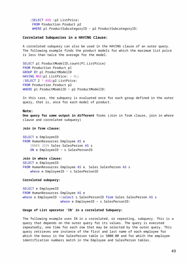
update Production.ProductInventory set modifiedDate=getdate() where productID =4

--Again see the table informationselect * from Production.ProductInventory order by productID

--Now set or execute the following statementset implicit_transactions off

--begin the transactionbegin TRANSACTIONupdate Production.ProductInventory set modifiedDate=getdate() where productID =4--to update permanentlycommit Transaction -- for Undorollback TRANSACTION

set implicit_transactions on

Important Note:

HumanResources.Employee table does not have departmentId field that has to be there.So do the following to relate the Employee table with department table and write query:

Step 1: Add departmentID column in Employee Table

alter table HumanResources.Employeeadd departmentID smallint

Step 2: Add FK constraint

alter table HumanResources.Employeeadd constraint FK foreign key (departmentID) References HumanResources.Department(DepartmentID)

Step 3: Update Employee table (Departmentid) with Departmentid of HumanResources.EmployeeDepartmentHistory table using common field employeeId

update HumanResources.Employee set HumanResources.Employee.departmentid=HumanResources.EmployeeDepartmentHistory.departmentidfrom HumanResources.EmployeeDepartmentHistory inner join HumanResources.Employeeon HumanResources.Employee.employeeid=HumanResources.EmployeeDepartmentHistory.employeeid

Action Queries: Before using action queries, always keep backup of previous version of data

Action queries are sql statements that can directly affect the underlying user tables by deleting, changing or adding data. There are many action queries in sql server which are explained here with examples. All other aspects of query which are already covered with simple query(DQL – Data Query Language would not be explained here. SO repeating the previous part is most for you.

Delete:This statement removes rows from a table or view.

Simple syntax of Delete query:

49

Deletr [from] Table_Name[Where <Condition>]

The DELETE statement may fail if it violates a trigger or tries to remove a row referenced by data in another table with a FOREIGN KEY constraint and the statement is canceled, an error is returned, and no rows are removed.

If you want to delete all the rows in a table, use the DELETE statement without specifying a WHERE clause, or use TRUNCATE TABLE. TRUNCATE TABLE is faster than DELETE and uses fewer system and transaction log resources

So, to delete rows from a table, you can use two SQL Statements:

1. Delete and 2. Truncate

Example:

Using DELETE with no WHERE clause:

DELETE FROM Sales.SalesPersonQuotaHistory

This query deletes all rows because there is no where clause to filter the rows to delete.

Using DELETE with WHERE clause:

The following example deletes all rows from the ProductCostHistory table in which the value in the StandardCost column is more than 1000.00.

DELETE FROM Production.ProductCostHistoryWHERE StandardCost > 1000

Using DELETE based on a subquery:

DELETE FROM Sales.SalesPersonQuotaHistory WHERE SalesPersonID IN (SELECT SalesPersonID FROM Sales.SalesPerson WHERE SalesYTD > 2500000)

Using DELETE based on a Join:

DELETE FROM Sales.SalesPersonQuotaHistory FROM Sales.SalesPersonQuotaHistory AS spqh INNER JOIN Sales.SalesPerson AS sp ON spqh.SalesPersonID = sp.SalesPersonIDWHERE sp.SalesYTD > 2500000.00

You have to mark onething important here. The from clause is repeated to delete data just to join two table and deciding to delete the records. Internal mechanism of the above query is like this:

First,

FROM Sales.SalesPersonQuotaHistory AS spqhINNER JOIN Sales.SalesPerson AS spON spqh.SalesPersonID = sp.SalesPersonID

Part is evaluated and WHERE sp.SalesYTD > 2500000.00 is evluated and at last DELETE FROM Sales.SalesPersonQuotaHistory is executed.

Using DELETE with the TOP clause:

50

DELETE TOP (2.5) PERCENT FROM Production.ProductInventory

This query deletes 2.5 percent of total number of records.

Delete statement deletes data from a table but does not show on screen. If you want to see the deleted output on the screen, use the following command.

DELETE dbo.NewTab OUTPUT DELETED.*where myid > 3

It will show output on the screen for your confirmation of deleted records.

Truncate command:

Truncate command deletes all records from table.

Truncate table aaa

Delete from table_nameWhere <Condition>

Drop table Table_Name

All of the above commands are used to delete data. Drop table command also delete the table, not only its data.

Difference in Delete , Truncate and Drop commands:

1. Truncate is DDL (Data Definition Language) statement.Delete is DML (Data Manipulation Language) statement.

2. Delete can be Rollbacked (Undo).Truncate cannot be Rollbacked.

3. Delete command uses condition to delete targeted rows.Truncate command does not use condition to delete rows. It deletes all rows from a table.

4. Delete command deletes rows one at a time and records an entry in Log file for each deleted row.Truncate command removes all data by dealocating the data pages used to store the table data and records page dealocation information int the Transaction Log file.So Truncate command is faster than Delete command.

Drop is a DDL command which is used to remove user defined database objects like table, view, prosedures and so.

If we drop a table, all dependencies are also deleted.

Suppose you deleted or updated some data that you should not.

For this, you have to use the following command:SET IMPLICIT_TRANSACTIONS ON When ON, SET IMPLICIT_TRANSACTIONS sets the connection into implicit transaction mode. When OFF, it returns the connection to autocommit transaction mode.

When a connection is in implicit transaction mode and the connection is not currently in a transaction, executing any of the following statements starts a transaction:

51

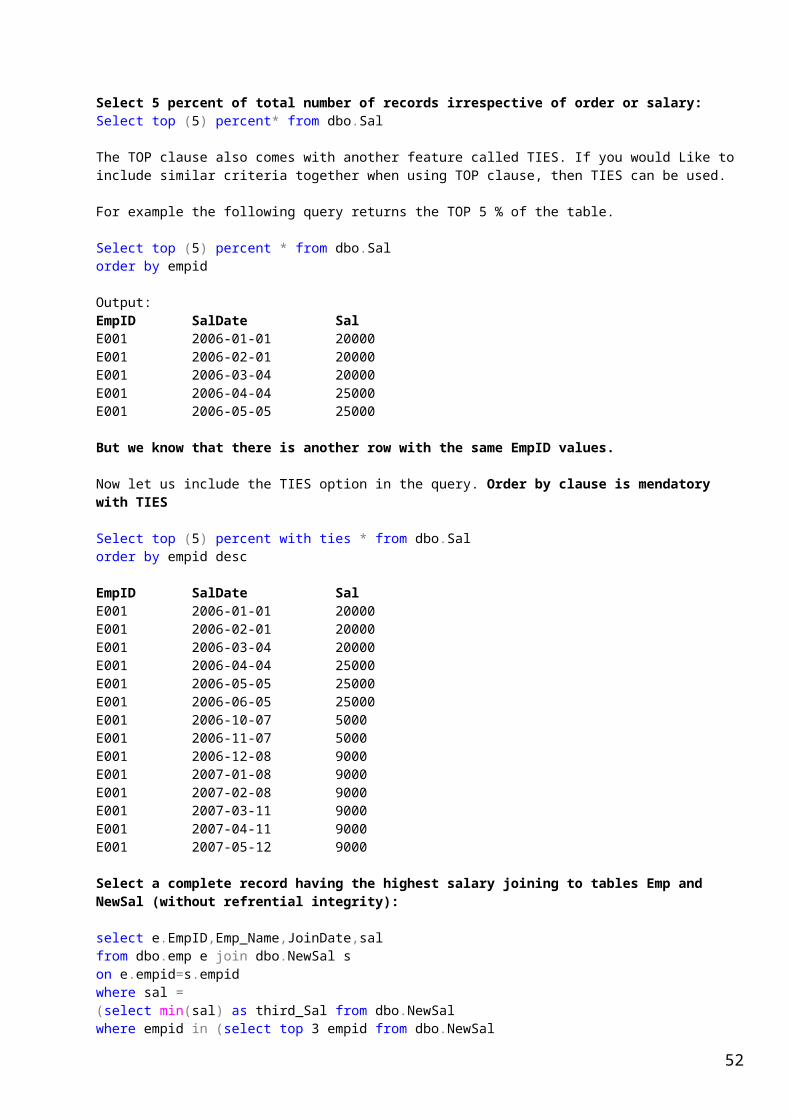
ALTER TABLE FETCH REVOKE

CREATE GRANT SELECT

DELETE INSERT TRUNCATE TABLE

DROP OPEN UPDATE

If the connection is already in an open transaction, the statements do not start a new transaction.

Transactions that are automatically opened as the result of this setting being ON must be explicitly committed or rolled back by the user at the end of the transaction. Otherwise, the transaction and all of the data changes it contains are rolled back when the user disconnects. After a transaction is committed, executing one of the statements above starts a new transaction.

Implicit transaction mode remains in effect until the connection executes a SET IMPLICIT_TRANSACTIONS OFF statement, which returns the connection to autocommit mode. In autocommit mode, all individual statements are committed if they complete successfully.

How can you do UNDO? For being at safe side, do implicit transaction mode ON as:

SET IMPLICIT_TRANSACTIONS ON

select * from AAA

It will select 7 records.

DELETE FROM AAA

It will delete all records.

ROLLBACK

It will do undo.

select * from AAA

Again, it will select 7 records.

DELETE FROM AAA

It will delete all records.Commit

It will save transaction.

After we commited any tractions, we cannot do rollback.

But SET IMPLICIT_TRANSACTIONS ON command works during the session. If we close sql server, it will ask to save the uncommited transactions. If we choose No, tranctions will not be saved.

To set implicit tractions permanently, follow the following steps:

Go to tool of Sql server management studio. Select option Expand the Query Execution Expand the SQL Server Select ANSI Check On “SET IMPLICIT_TRANSACTIONS”

Update52

An update statement can Change existing data in a table or view. If an update to a row violates a constraint or rule, violates the NULL setting for the column, or the new value is an incompatible data type, the statement is canceled, an error is returned, and no records are updated.

When an UPDATE statement encounters an arithmetic error (overflow, divide by zero, or a domain error) during expression evaluation, the update is not performed and an error message is returned.

Syntax to update:

Update TABLE_NAMESET FIELD_NAME = VALUEWHERE <condition>

Example of simple updateThe following examples show how all rows can be affected when a WHERE clause is not used to specify the row or rows to update.

This example updates the values in the Bonus, CommissionPct, and SalesQuota columns for all rows in the SalesPerson table.

UPDATE Sales.SalesPersonSET Bonus = 6000, CommissionPct = .10, SalesQuota = NULL

You can also use computed values in an UPDATE statement. The following example doubles the value in the ListPrice column for all rows in the Product table.

UPDATE Production.ProductSET ListPrice = ListPrice * 2

Using the UPDATE statement with a WHERE clause

UPDATE Production.ProductSET Color = 'Metallic Red'WHERE Name LIKE 'Road-250%' AND Color = 'Red'

Using the UPDATE statement with information from another table

The following example modifies the SalesYTD column in the SalesPerson table to reflect the most recent sales recorded in the SalesOrderHeader table.

UPDATE Sales.SalesPersonSET SalesYTD = SalesYTD + SubTotalFROM Sales.SalesPerson AS spJOIN Sales.SalesOrderHeader AS so ON sp.SalesPersonID = so.SalesPersonID AND so.OrderDate = (SELECT MAX(OrderDate) FROM Sales.SalesOrderHeader WHERE SalesPersonID = sp.SalesPersonID)

The above example assumes that only one sale is recorded for a specified salesperson on a specific date and that updates are current. If more than one sale for a specified salesperson can be recorded on the same day, the above query does not work correctly. The example runs without error, but each SalesYTD value is updated with only one sale, regardless of how many sales actually occurred on that day. This is because a single UPDATE statement never updates the same row two times.

In the situation in which more than one sale for a specified salesperson can occur on the same day, all the sales for each sales person must be aggregated together within the UPDATE statement.

53

For example:

UPDATE Sales.SalesPersonSET SalesYTD = SalesYTD + (SELECT SUM(so.SubTotal) FROM Sales.SalesOrderHeader AS so WHERE so.OrderDate = (SELECT MAX(OrderDate) FROM Sales.SalesOrderHeader AS so2 WHERE so2.SalesPersonID = so.SalesPersonID) AND Sales.SalesPerson.SalesPersonID = so.SalesPersonID GROUP BY so.SalesPersonID)

Using UPDATE with the TOP clause

The following example updates the VacationHours column by 25 percent for 10 random rows in the Employee table.

UPDATE TOP (10) HumanResources.EmployeeSET VacationHours = VacationHours * 1.25

Another example:

UPDATE TOP (3) dbo.Sal SET Sal = 25000where sal in (select min(sal) from dbo.Sal)

Above query will update three records in the table. We can also use TOP percent clause. Following is the delete statement which deletes 20 percent records from the table.

Use Case statement with Update statement:

UPDATE HumanResources.EmployeeSET VacationHours = ( CASE WHEN ((VacationHours - 10.00) > 0) THEN VacationHours - 40 ELSE (VacationHours - 20.00) END )

Using UPDATE with the OUTPUT clause (Do this after you study of Triggers)

The following example updates the VacationHours column in the Employee table by 25 percent for the first 10 rows. The OUTPUT clause returns the value of VacationHours that exists before applying the UPDATE statement in the DELETED.VacationHours column and the updated value in the INSERTED.VacationHours column to the @MyTableVar table variable.

Two SELECT statements follow that return the values in @MyTableVar and the results of the update operation in the Employee table. Note the results in the INSERTED.ModifiedDate column are different from the values in the ModifiedDate column in the Employee table. This is because the AFTER UPDATE trigger that updates the value of ModifiedDate to the current date is defined on the Employee table. However, the columns returned from OUTPUT reflect the data before triggers are fired.

DECLARE @MyTableVar table( EmpID int NOT NULL, OldVacationHours int, NewVacationHours int, ModifiedDate datetime);UPDATE TOP (10) HumanResources.Employee

54

SET VacationHours = VacationHours * 1.25 OUTPUT INSERTED.EmployeeID, DELETED.VacationHours, INSERTED.VacationHours, INSERTED.ModifiedDateINTO @MyTableVar--Display the result set of the table variable.SELECT EmpID, OldVacationHours, NewVacationHours, ModifiedDateFROM @MyTableVar;

--Display the result set of the table.--Note that ModifiedDate reflects the value generated by an--AFTER UPDATE trigger.SELECT TOP (10) EmployeeID, VacationHours, ModifiedDateFROM HumanResources.Employee

Using OUTPUT INTO with from_table_name in an UPDATE statement

The following example updates the ScrapReasonID column in the WorkOrder table for all work orders with a specified ProductID and ScrapReasonID. The OUTPUT INTO clause returns values from the table being updated (WorkOrder) and also from the Product table. The Product table is used in the FROM clause to specify the rows to update. Because the WorkOrder table has an AFTER UPDATE trigger defined on it, the INTO keyword is required.

Note: To see the output of the following query, you have to execute the whole statement as batch. You will hardly do implement such update statements in your daily activity. Because you cannot save the data in Table Varible. This is shown here only to give internal percepton of Update statement.

DECLARE @MyTestVar table ( OldScrapReasonID int NOT NULL, NewScrapReasonID int NOT NULL, WorkOrderID int NOT NULL, ProductID int NOT NULL, ProductName nvarchar(50)NOT NULL);UPDATE Production.WorkOrderSET ScrapReasonID = 4OUTPUT DELETED.ScrapReasonID, INSERTED.ScrapReasonID, INSERTED.WorkOrderID, INSERTED.ProductID, p.Name INTO @MyTestVarFROM Production.WorkOrder AS wo INNER JOIN Production.Product AS p ON wo.ProductID = p.ProductID AND wo.ScrapReasonID= 16 AND p.ProductID = 733;SELECT OldScrapReasonID, NewScrapReasonID, WorkOrderID, ProductID, ProductName FROM @MyTestVar;

Insert:

Insert Statement adds a new row to a table or a view.

We can insert records in a table in many ways:

Insert data through application interface that we don’t discuss here. Insert data through simple insert statement Insert data through view Insert data using the SELECT INTO Bulk insert

55

Import

Simple INSERT statement:

Syntax:

INSERT [INTO] TABLE_NAME [<FIELD_LIST>]VALUES <VALUE_LIST in same sequence of field list>

Example:

INSERT INTO Production.UnitMeasureVALUES ('RB', 'Square Feet_2', GETDATE())

OR

INSERT Production.UnitMeasureVALUES ('RB', 'Square Feet_2', GETDATE())

Note: If we are inserting values in all fields in same sequence of fields, no need to specify the field list in INSERT statement. We have to specify field list in two situations. First, though we are going to insert values for all fields but we don’t know the sequence of fields, then we have to specify all fields in any sequence. Then insert values in same sequence as of fields’ sequence.

Second, if we are not inserting values for nullable fields.

The above query inserts values for all fields in proper sequence. So no need field list in insert statement.

Inserting data that is not in the same order as the table columns

The following example uses column_list to explicitly specify the values that are inserted into each column. The column order in the UnitMeasure table is UnitMeasureCode, Name, ModifiedDate; however, the columns are not listed in that order in column_list.

INSERT INTO Production.UnitMeasure (Name, UnitMeasureCode, ModifiedDate)VALUES ('Square Yards', 'Y2', GETDATE())

Inserting data with fewer values than columns

The following example shows inserting rows into a table with columns that automatically generate a value or have a default value. The INSERT statements insert rows that contain values for some of the columns but not all. In the last INSERT statement, no columns are specified and only the default values are inserted.

No need to insert value for Identity column. Database automatically inserts values in defined sequence.

If default values are assigned for columns at table design time, Database automatically inserts values for such column if we have not supplied any value for the columns. If we supply value for the default column, then default values are overridden.

Do the following coding in your test database:

--It thecks the table in the database and deletes first for creating a new table with the same nameIF OBJECT_ID ('dbo.T1') IS NOT NULL DROP TABLE dbo.T1

56

CREATE TABLE dbo.T1 ( ID int IDENTITY, FName varchar(30), Address varchar(50)CONSTRAINT default_Add DEFAULT ('I-259,Gali No. 8, Jaitpur, N.D. 110044'), Job_Profile varchar(40) NULL)

Way of inserting values with Identity Property and Default values:

INSERT INTO dbo.T1 (FName) VALUES ('Rabi')

INSERT INTO dbo.T1 (FName, Job_Profile) VALUES ('Hari', 'MIS')

INSERT INTO dbo.T1 (FName, Address,Job_Profile) VALUES ('Rajwant','Chirag Delhi','Reporting')

INSERT INTO T1 DEFAULT VALUES

Inserting data into a ‘uniqueidentifier’ column by using NEWID()in SQL Server 2005 and above:

The following example uses the NEWID() function to obtain a GUID for column_2. Unlike for identity columns, the Database Engine does not automatically generate values for columns with the uniqueidentifier data type, as shown by the second INSERT statement.

IF OBJECT_ID ('dbo.T2') IS NOT NULL DROP TABLE dbo.T2

CREATE TABLE dbo.T2 ( ID int IDENTITY (100,1), Unique_Val uniqueidentifier,)

INSERT INTO dbo.T2 (Unique_Val) VALUES (NEWID())

--This statement inserts value for Identity column and null as default value for Unique_Val column INSERT INTO T2 DEFAULT VALUES

SELECT *FROM dbo.T2

Inserting data into a table through a view

IF OBJECT_ID ('dbo.T1') IS NOT NULL DROP TABLE dbo.T1;

CREATE TABLE dbo.T1 ( ID int IDENTITY, FName varchar(30),

Address varchar(50)CONSTRAINT default_Add DEFAULT ('I-259,Gali No. 8, Jaitpur, N.D. 110044'), Job_Profile varchar(40) NULL)

INSERT INTO dbo.T1 (FName)

57

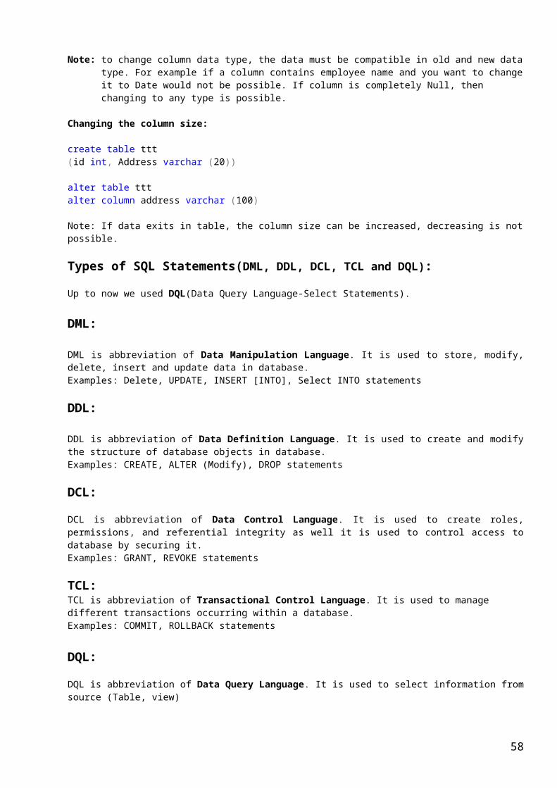
VALUES ('Rabi')

INSERT INTO dbo.T1 (FName, Job_Profile) VALUES ('Hari', 'MIS')

INSERT INTO dbo.T1 (FName, Address,Job_Profile) VALUES ('Rajwant','Chirag Delhi','Reporting')

INSERT INTO T1 DEFAULT VALUES

CREATE VIEW v1 ASSELECT * FROM t1

INSERT INTO v1 (FName, Address,Job_Profile) VALUES ('Kuldeep','Chirag Delhi','Operation')

SELECT * FROM v1

Insert data using the SELECT (Append Data)

First, create the table in your test database

IF OBJECT_ID ('dbo.EmployeeSales') IS NOT NULL DROP table dbo.EmployeeSales

CREATE TABLE dbo.EmployeeSales( DataSource varchar(20) NOT NULL, EmployeeID varchar(11) NOT NULL, LastName varchar(40) NOT NULL, SalesDollars money NOT NULL)

INSERT INTO dbo.EmployeeSales SELECT 'SELECT', e.EmployeeID, c.LastName, sp.SalesYTD FROM HumanResources.Employee AS e INNER JOIN Sales.SalesPerson AS sp ON e.EmployeeID = sp.SalesPersonID INNER JOIN Person.Contact AS c ON e.ContactID = c.ContactID WHERE e.EmployeeID LIKE '2%' ORDER BY e.EmployeeID, c.LastName

select * from dbo.EmployeeSales

Inserting data by using the TOP clause

The following example creates the NewEmployee table and inserts address data for the top 10 employees from the Employee table into it. The SELECT statement is then executed to verify the contents of the NewEmployee table.

IF OBJECT_ID ('HumanResources.NewEmployee') IS NOT NULL DROP TABLE HumanResources.NewEmployee

CREATE TABLE HumanResources.NewEmployee( EmployeeID int NOT NULL, LastName nvarchar(50) NOT NULL, FirstName nvarchar(50) NOT NULL, Phone Phone NULL, AddressLine1 nvarchar(60) NOT NULL, City nvarchar(30) NOT NULL, State nchar(3) NOT NULL, PostalCode nvarchar(15) NOT NULL, CurrentFlag Flag)

58

INSERT TOP (10) INTO HumanResources.NewEmployee SELECT e.EmployeeID, c.LastName, c.FirstName, c.Phone, a.AddressLine1, a.City, sp.StateProvinceCode, a.PostalCode, e.CurrentFlag FROM HumanResources.Employee e INNER JOIN HumanResources.EmployeeAddress AS ea ON e.EmployeeID = ea.EmployeeID INNER JOIN Person.Address AS a ON ea.AddressID = a.AddressID INNER JOIN Person.StateProvince AS sp ON a.StateProvinceID = sp.StateProvinceID INNER JOIN Person.Contact as c ON e.ContactID = c.ContactID

SELECT EmployeeID, LastName, FirstName, Phone, AddressLine1, City, State, PostalCode, CurrentFlagFROM HumanResources.NewEmployee

Using WITH Common Table Expression with an INSERT statement(Do this after studying CTE)

The following example creates the NewEmployee table. A common table expression (EmployeeTemp) defines the rows to be inserted into the NewEmployee table. The INSERT statement references the columns in the common table expression.

IF OBJECT_ID ('HumanResources.NewEmployee') IS NOT NULL DROP TABLE HumanResources.NewEmployee;

CREATE TABLE HumanResources.NewEmployee( EmployeeID int NOT NULL, LastName nvarchar(50) NOT NULL, FirstName nvarchar(50) NOT NULL, Phone Phone NULL, AddressLine1 nvarchar(60) NOT NULL, City nvarchar(30) NOT NULL, State nchar(3) NOT NULL, PostalCode nvarchar(15) NOT NULL, CurrentFlag Flag)

WITH EmployeeTemp (EmpID, LastName, FirstName, Phone, Address, City, StateProvince, PostalCode, CurrentFlag)AS (SELECT e.EmployeeID, c.LastName, c.FirstName, c.Phone, a.AddressLine1, a.City, sp.StateProvinceCode, a.PostalCode, e.CurrentFlag FROM HumanResources.Employee e INNER JOIN HumanResources.EmployeeAddress AS ea ON e.EmployeeID = ea.EmployeeID INNER JOIN Person.Address AS a ON ea.AddressID = a.AddressID INNER JOIN Person.StateProvince AS sp ON a.StateProvinceID = sp.StateProvinceID INNER JOIN Person.Contact as c ON e.ContactID = c.ContactID )INSERT INTO HumanResources.NewEmployee SELECT EmpID, LastName, FirstName, Phone, Address, City, StateProvince, PostalCode, CurrentFlag FROM EmployeeTemp

59

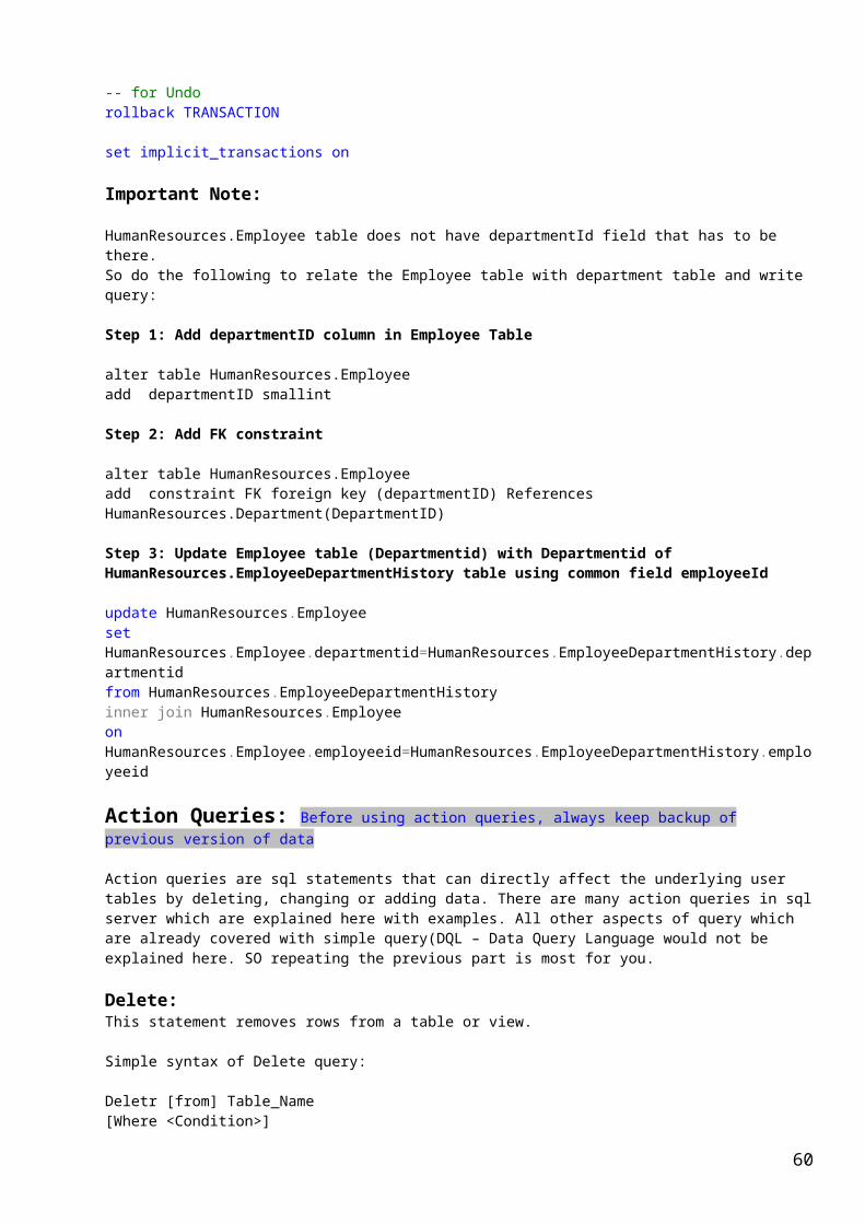
select * from HumanResources.NewEmployee

UNDO in insert statement

set implicit_transactions ON

INSERT INTO Production.UnitMeasureVALUES ('RB', 'Square Feet_2', GETDATE())

commit

select * from Production.UnitMeasure

delete from Production.UnitMeasurewhere name = 'Square Feet_2'

rollback

Bulk Insert / Append

This command loads / inserts or appends data from a data file into a database table or view in a user-specified format.

First, create a table with the same fields as that of file.Then execute the following code to insert tab delimited data in table. Tab is the default delamitor.

Note: File should not have field(heading), only data is required.

BULK INSERT bul FROM 'C:\Documents and Settings\Administrator\Desktop\p.txt'

If fields are delamited by other delimiter, use the following syntax:

For semicolon:

BULK INSERT Bul FROM 'C:\Documents and Settings\Administrator\Desktop\p.txt' WITH ( FIELDTERMINATOR = ';', ROWTERMINATOR = '\n' )

To fix the starting row:

BULK INSERT Bul FROM 'C:\Documents and Settings\Administrator\Desktop\p.txt' WITH ( FIELDTERMINATOR = ';', ROWTERMINATOR = '\n' ,FIRSTROW = 2)

For CSV file:

BULK INSERT bul FROM 'C:\Documents and Settings\Administrator\Desktop\p.csv' WITH ( FIRSTROW = 2, MAXERRORS = 0, FIELDTERMINATOR = ',',

60

ROWTERMINATOR = '\n' )

With maximum bulk insert property

BULK INSERT Bul --Bul is tableFROM 'C:\Documents and Settings\Administrator\Desktop\p.txt' WITH ( FIELDTERMINATOR = ';', ROWTERMINATOR = '\n', FIRSTROW = 3,LASTROW = 5,BATCHSIZE = 2,CHECK_CONSTRAINTS,FIRE_TRIGGERS,KEEPIDENTITY,KEEPNULLS,MAXERRORS = 100,ROWS_PER_BATCH=10,TABLOCK)

In general, following properties are used:

BULK INSERT Bul --Bul is tableFROM 'C:\Documents and Settings\Administrator\Desktop\p.txt' WITH ( FIELDTERMINATOR = ';', ROWTERMINATOR = '\n', CHECK_CONSTRAINTS,FIRE_TRIGGERS,TABLOCK)

Explanation of all property:

BATCHSIZE = batch_size:

Specifies the number of rows in a batch. Each batch is copied to the server as one transaction. If this fails, SQL Server commits or rolls back the transaction for every batch. By default, all data in the specified data file is one batch.

CHECK_CONSTRAINTS:

Specifies that all constraints on the target table or view must be checked during the bulk import operation. Without the CHECK_CONSTRAINTS option, any CHECK constraints are ignored, and after the operation the constraint on the table is marked as not-trusted.

Note: UNIQUE, PRIMARY KEY, FOREIGN KEY, or NOT NULL constraints are always enforced. At some point, you must examine the constraints on the whole table. If the table was non-empty before the bulk import operation, the cost of revalidating the constraint may exceed the cost of applying CHECK constraints to the incremental data.

A situation in which you might want constraints disabled (the default behavior) is if the input data contains rows that violate constraints. With CHECK constraints disabled, you can import the data and then use Transact-SQL statements to remove the invalid data.

61

Note: The MAXERRORS option does not apply to constraint checking.

FIELDTERMINATOR = 'field_terminator':

Specifies the field terminator to be used for char and widechar data files. The default field terminator is \t (tab character).

FIRSTROW = first_row:

Specifies the number of the first row to load. The default is the first row in the specified data file.

FIRE_TRIGGERS:

Specifies that any insert triggers defined on the destination table execute during the bulk load operation. If triggers are defined for INSERT operations on the target table, they are fired for every completed batch.

If FIRE_TRIGGERS is not specified, no insert triggers execute.

KEEPIDENTITY:

Specifies that identity value or values in the imported data file are to be used for the identity column. If KEEPIDENTITY is not specified, the identity values for this column are verified but not imported and SQL Server automatically assigns unique values based on the seed and increment values specified during table creation. If the data file does not contain values for the identity column in the table or view, use a format file to specify that the identity column in the table or view is to be skipped when importing data; SQL Server automatically assigns unique values for the column.

KEEPNULLS:

Specifies that empty columns should retain a null value during the bulk load operation, instead of having any default values for the columns inserted.

KILOBYTES_PER_BATCH = kilobytes_per_batch:

Specifies the approximate number of kilobytes (KB) of data per batch as kilobytes_per_batch. By default, KILOBYTES_PER_BATCH is unknown.

LASTROW = last_row:

Specifies the number of the last row to load. The default is 0, which indicates the last row in the specified data file.

MAXERRORS = max_errors:

Specifies the maximum number of syntax errors allowed in the data before the bulk load operation is canceled. Each row that cannot be imported by the bulk load operation is ignored and counted as one error. If max_errors is not specified, the default is 10.

Note: The MAX_ERRORS option does not apply to constraint checks or to converting money and bigint data types.

ROWS_PER_BATCH = rows_per_batch:

Indicates the approximate number of rows of data in the data file.

By default, all the data in the data file is sent to the server as a single transaction, and the number of rows in the batch is unknown to the query

62

optimizer. If you specify ROWS_PER_BATCH (with a value > 0) the server uses this value to optimize the bulk import operation. The value specified for ROWS_PER_BATCH should approximately the same as the actual number of rows.

ROWTERMINATOR = 'row_terminator':

Specifies the row terminator to be used for char and widechar data files. The default row terminator is \n (newline character).

TABLOCK:

Specifies that a table-level lock is acquired for the duration of the bulk load operation. A table can be loaded concurrently by multiple clients if the table has no indexes and TABLOCK is specified. By default, locking behavior is determined by the table option table lock on bulk load. Holding a lock for the duration of the bulk load operation reduces lock contention on the table, significantly improving performance.

Insert into (Append / Insert)

To append data in a database table from another table, use the following command:

Insert into Employee_HistorySelect * from Employees

Or

Insert into Employee_History (Field1,Field2,Field3)Select Field1,Field2,Field3 from Employees

Note: While inserting data in a table, keep few things in mind that the field list should have compatible data type, size and non Null column should be supplied with value.

To create table based on another table:

Select * into new_Table from old_table

This command will copy the entire data from old table to new table.

To limite the data, we should provide where or having clause.

The following command copies only structure of a table:

Select * into New_Table from Old_tableWhere 1=2

System defined functions (Date, Math, String and Conversion):

Basically functions are of two types:

Built-In functions User-defined functions.

Let’s begin with Built-In functions.

Built-in functions are provided by SQL Server to help you perform a variety of operations. They cannot be modified. You can use built-in functions in Transact-SQL statements to:

Access information from SQL Server system tables without accessing the system tables directly.

Perform common tasks such as SUM, GETDATE, or IDENTITY.

63

Built-in functions return either scalar or table data types. For example, @@ERROR returns 0 if the last Transact-SQL statement executed successfully. If the statement generated an error, @@ERROR returns the error number. And the function SUM(parameter) returns the sum of all the values for the parameter.

Types of Built-in functions: Scalar functions Aggregate Functions Ranking Functions

Scalar Function:Scalar functions operate on a single value and then return a single value. Scalar functions can be used wherever an expression is valid.

Types of Scalar Functions:

Function category Description

Date and Time Functions

Perform operations on a date and time input values and return string, numeric, or date and time values.

String Functions Perform operations on a string (char or varchar) input value and return a string or numeric value.

System Functions Perform operations and return information about values, objects, and settings in an instance of SQL Server.

Metadata Functions

Return information about the database and database objects.

Security Functions

Return information about users and roles.

Mathematical Functions

Perform calculations based on input values provided as parameters to the functions, and return numeric values.

Date and Time Functions:{Note: SQL Server accepts or recognizes Date value in the following format only:

Alphabetic format: ‘April 15, 2009’Numeric Format: ‘4/15/2009’

String Format: ‘20090415’}

The Date time function is used to perform an operation on a date and time value and return a string, numeric, or date and time value.

There are many forms of date time functions. Let’s go one by one with example:

Datepart Abbreviations

year yy, yyyy

quarter qq, q

month mm, m

dayofyear dy, y

day dd, d

week wk, ww

weekday dw, w

hour hh

minute mi, n

64

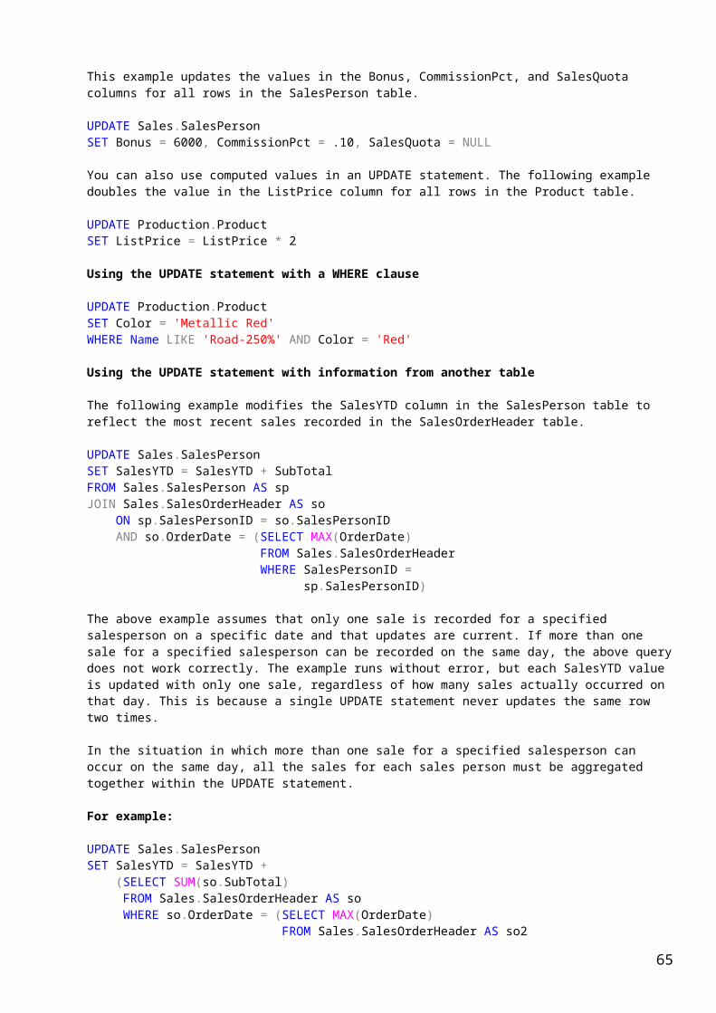
second ss, s

millisecond ms

GateDate(): This function returns current system date and time.

SELECT GETDATE()===========2009-12-22 20:08:51.543

DATEADD:

This function adds a certain period of time to the existing date and time value:

Syntax: DATEADD (datepart, number, date)

SELECT DATEADD(MONTH, 6, GETDATE())AS '6_months_from_now'

2010-06-22 19:36:18.937

Month or mm

SELECT DATEADD(mm, 6, GETDATE())AS '6_months_from_now'

DATEDIFF:

Syntax: DATEDIFF (datepart, startdate, enddate)

This function returns difference between two date values.

SELECT orderDate,getdate(),DATEDIFF(day, OrderDate, GETDATE()) AS NumberOfDaysFROM Sales.SalesOrderHeader

Note: Old date should be before the new date in parameter sequence.

DATENAME:

Syntax: DATENAME (datepart ,date)

The DATENAME function returns the name of the portion of the date and time Value. Just like the DATEPART function, the DATENAME function accepts two parameters: the portion of the date that you want to retrieve and the date. The DATENAME function can be used to retrieve any of the following: name of the year, quarter, and month, day of the year, day, week, weekday, hour, minute, second, or millisecond of the specified date.

See some examples:SELECT Datename(dayofyear, GETDATE()) AS NumberOfDays============365

SELECT Datename(quarter, GETDATE()) AS NumberOfDays============4

SELECT Datename(Month, GETDATE()) AS NumberOfDays============December

SELECT Datename(weekday, GETDATE()) AS NumberOfDays============Tuesday

DATEPART:Syntxa: DATEPART (datepart , date)

65

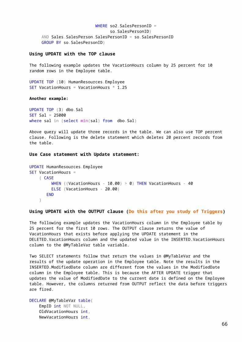
This function returns an integer that represents the specified datepart of the specified date.

SELECT DATEPART(month, GETDATE()) AS 'Month Number'==========12

SELECT DATEPART(Year, '4/15/2006') AS 'Month Number'========2006

DAY, MONTH, and YEAR Functions:

DAY, MONTH and YEAR functions accept a single date value as a parameter and returns respective portions of the date as an integer. The following example shows how various portions of the date and time value can be retrieved using these functions:

SELECT DAY('January 1, 2007') as Day, MONTH('January 1, 2007') as Month, YEAR('January 1, 2007')as Year

Day Month Year==========================================1 1 2007

Customized Date formats in select statement:Note: You will see some string functions while formatting date.

Date Format SQL Statement Sample Output

MM/DD/YY SELECT CONVERT(VARCHAR(10), '12/15/2009', 1) AS [MM/DD/YY] 11/23/98

MM/DD/YYYY SELECT CONVERT(VARCHAR(10), GETDATE(), 101) AS [MM/DD/YYYY] 11/23/1998

YY.MM.DD SELECT CONVERT(VARCHAR(8), GETDATE(), 2) AS [YY.MM.DD] 72.01.01

YYYY.MM.DD SELECT CONVERT(VARCHAR(10), GETDATE(), 102) AS [YYYY.MM.DD] 1972.01.01

DD/MM/YY SELECT CONVERT(VARCHAR(8), GETDATE(), 3) AS [DD/MM/YY] 19/02/72

DD/MM/YYYY SELECT CONVERT(VARCHAR(10), GETDATE(), 103) AS [DD/MM/YYYY] 19/02/1972

DD.MM.YY SELECT CONVERT(VARCHAR(8), GETDATE(), 4) AS [DD.MM.YY] 25.12.05

DD.MM.YYYY SELECT CONVERT(VARCHAR(10), GETDATE(), 104) AS [DD.MM.YYYY] 25.12.2005

DD-MM-YY SELECT CONVERT(VARCHAR(8), GETDATE(), 5) AS [DD-MM-YY] 24-01-98

DD-MM-YYYY SELECT CONVERT(VARCHAR(10), GETDATE(), 105) AS [DD-MM-YYYY] 24-01-1998

HH:MM:SS SELECT CONVERT(VARCHAR(8), GETDATE(), 108) 03:24:53

MM-DD-YY SELECT CONVERT(VARCHAR(8), GETDATE(), 10) AS [MM-DD-YY] 01-01-06

MM-DD-YYYY SELECT CONVERT(VARCHAR(10), GETDATE(), 110) AS [MM-DD-YYYY] 01-01-2006

You can try 1 to 130 integer value for style parameter.

Important String Functions:

Left: This function is used to retrieve the left portion of a string.

select left('ABCDEFG',4) as fourCharFromLeft : ABCD

RIGHT: This function is used to retrieve the right portion of a string.

select Right('ABCDEFG',4) as fourCharFromRight : DEFG LTRIM and RTRIM Functions:

LTRIM function removes the leading blanks. Similarly the RTRIM function removes the trailing spaces. For instance

66

select Ltrim(' ABCDEFG') as LeadingSpaceRemoved : ABCDEFG……………

select Rtrim(' ABCDEFG ') as TrailingSpaceRemoved : ……………………ABCDEFG

To remove space from both sides:

select Ltrim(Rtrim(' ABCDEFG ')) as R : ABCDEFG

SUBSTRING:

SUBSTRING function retrieves a portion of the string starting at the specified Position and number of characters.

The syntax is:

SUBSTRING(string, starting_character_number, number_of_characters_to_return)

Substring is equivalent of MID function in VBA.

SELECT LastName, SUBSTRING(LastName, 1, 1) AS InitialFROM Person.ContactWHERE LastName like 'Barl%'ORDER BY LastName

Output:LastName Initial======= =======Barley BBarlow B

The following example will retrieve four characters from the employee last names, starting at the third character:

SELECT lastName,SUBSTRING(LastName, 3, 4) AS PortionOfLastName FROM Person.Contact

LastName PortionOfLastName======== ==================Achong hongAbel elAbercrombie ercrAcevedo evedAckerman kerm

REVERSE:

The REVERSE function gives you a mirror image of a given string.

SELECT REVERSE('Rabi') AS MirrorImage : ibaR

CHARINDEX:

Transact-SQL supports two functions for finding an occurrence of a particular character (or number of characters) within a string: CHARINDEX and PATINDEX. CHARINDEX finds the starting position of a single character or string within a given column (or variable). In addition, if you suspect that the value you are searching for might occur multiple times within a given string you can specify the character number at which you want to start searching.

The syntax of the function is:

CHARINDEX(search value, string[, starting search location])

67

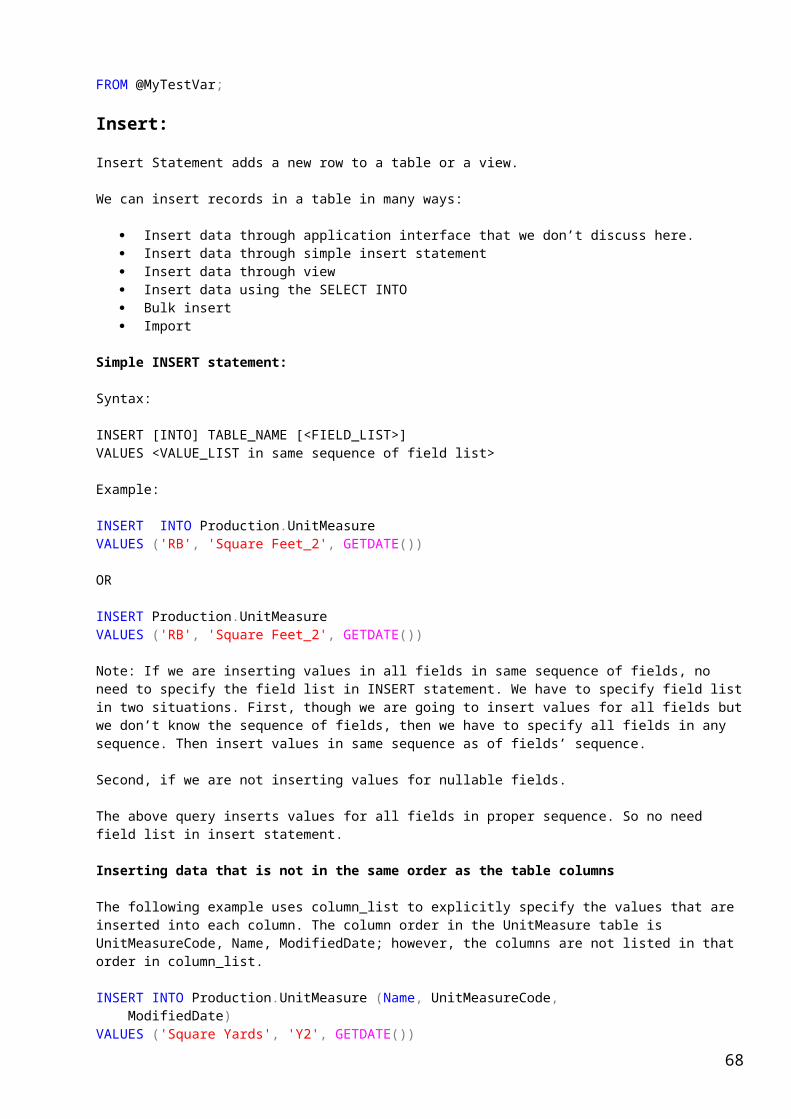
This function is equivalent of Find function in Excel or instr in VBA.

It returns the starting position of the specified expression in a character string.

Example:

select CHARINDEX('L', 'Rabi Lal Puri') as Position: Returns 6

select CHARINDEX('l', 'Rabi Lal Puri',2) as Position: Returns 8

Pull FirstName, middleName and LastName using left, right, Substring and CHARINDEX function:

Retrieve FirstName:select left('Rabi Lal Puri',CHARINDEX(' ', 'Rabi Lal Puri')-1) as FirstName

Retrieve Middle Name:

select substring('Rabi Lal Puri',CHARINDEX(' ', 'Rabi Lal Puri')+1,CHARINDEX(' ','Rabi Lal Puri',CHARINDEX(' ', 'Rabi Lal Puri')+1)-CHARINDEX(' ','Rabi Lal Puri')-1) as MiddleName

Retrieve Last Name:

select Right('Rabi Lal Puri',len('Rabi Lal Puri')-(Charindex(' ','Rabi Lal Puri',Charindex(' ','Rabi Lal Puri')+1)))as Last_name

REPLACE:REPLACE function replaces some characters within a string with another set of characters.

The syntax is:

REPLACE(string expression, value to be replaced, replacing value)

select REPLACE('Rabi Lal Puri', 'Puri', 'Rai')

Output: Rabi Lal RaiREPLICATE:

The REPLICATE function repeats a given string specified number of times.

The syntax is: REPLICATE(string, number of times).

select REPLICATE ('*', 10)+'Rabi'+REPLICATE ('*', 10)

Output: **********Rabi**********

UPPER and LOWER:

UPPER and LOWER functions change the case of the query's output. Both functions accept a string expression as the only argument.

Select Upper('rabi') as UpperCase , Lower('RABI')as LowerCase

UpperCase LowerCase========= =========RABI rabi

ASCII:

ASCII function returns the ASCII code value of the leftmost character of a string.

68

SELECT ASCII('A') AS UpperCase, ASCII('a') AS LowerCase

Output: 65 97

CHAR:

The CHAR function does the opposite of ASCII - it returns an alphanumeric equivalent of an ASCII code.

SELECT CHAR(65) AS UpperCase, CHAR(97) AS LowerCase

Output: A a

Important System Functions:

CASE:

CASE is typically classified as a system function; however, it could also be considered as a statement. Case statement is used for conditional output.

The following query attempts to specify the salary level for each job title within Adventure Works DW database:

SELECT DISTINCT TITLE,SALARYRANGE = CASE

WHEN TITLE LIKE 'Chief%' THEN 'unlimited'WHEN TITLE LIKE '%manager%' THEN '100K to 250K'WHEN TITLE LIKE '%assistant%' THEN '20K to 40K'WHEN TITLE LIKE '%supervisor%' THEN '50K to 65K'WHEN TITLE LIKE '%technician%' THEN '30K to 60K'WHEN TITLE LIKE 'vice president%' THEN '250K to 500K'ELSE 'unknown'

ENDFROM DIMEMPLOYEE

TITLE SALARYRANGE======= ===========Accountant unknownAccounts Manager 100K to 250KChief Executive Officer unlimitedNetwork Manager 100K to 250KPurchasing Assistant 20K to 40KPurchasing Manager 100K to 250KVice President of Sales 250K to 500K

The other variation of CASE, which is sometimes referred to as the searched CASE, evaluates a Boolean expression and returns different values accordingly. For instance, we could use the searched CASE to categorize the top internet customers within Adventure Works DW database as follows:

SELECT FirstName + ', ' + LastName AS FullName, CustomerCategory = CASE

WHEN SUM(SalesAmount) < 12000 THEN 'SILVER' WHEN SUM(SalesAmount) BETWEEN 12000 AND 13250 THEN 'GOLD' WHEN SUM(SalesAmount) BETWEEN 13250 AND 15000 THEN 'PLATINUM' ELSE 'CREAM OF THE CROP'

END, SUM(SalesAMount) AS TotalOrders FROM dimCustomer a INNER JOIN FactInternetSales b ON a.CustomerKey = b.CustomerKey GROUP BY FirstName + ', ' + LastName HAVING SUM(SalesAmount) >=11000

COALESCE:

69

This function returns the first Non_NULL expression among its arguments. If all arguments are NULL, COALESCE returns NULL.

To understand the usage of this function, create the following table in your test database:

CREATE TABLE wages( emp_id Int identity, hourly_wage decimal NULL, salary decimal NULL, commission decimal NULL, num_sales Int NULL)

Now insert the following data:

emp_id hourly_wage salary commission num_sales ======= ============ ====== ========== =========1 10 NULL NULL NULL2 20 NULL NULL NULL3 30 NULL NULL NULL4 40 NULL NULL NULL5 NULL 10000 NULL NULL6 NULL 20000 NULL NULL7 NULL 30000 NULL NULL8 NULL 40000 NULL NULL9 NULL NULL 15000 310 NULL NULL 25000 211 NULL NULL 20000 612 NULL NULL 14000 4

Run the following query to use the COALESCE function:

select emp_id ,hourly_wage,salary,commission,num_sales,COALESCE(hourly_wage * 40 * 52, salary, commission * num_sales) AS 'Total Salary'FROM wages

Output:

emp_id hourly_wage salary commission num_sales Total Salary======= ============ ====== ========== ========= ============1 10 NULL NULL NULL 208002 20 NULL NULL NULL 416003 30 NULL NULL NULL 624004 40 NULL NULL NULL 832005 NULL 10000 NULL NULL 100006 NULL 20000 NULL NULL 200007 NULL 30000 NULL NULL 300008 NULL 40000 NULL NULL 400009 NULL NULL 15000 3 4500010 NULL NULL 25000 2 5000011 NULL NULL 20000 6 12000012 NULL NULL 14000 4 56000

Note:COALESCE (expression1...n) is equivalent to this CASE function:

CASE WHEN (expression1 IS NOT NULL) THEN expression1 WHEN (expressionN IS NOT NULL) THEN expressionN ELSE NULLEND

70

NULLIF:

This function returns a null value if two specified expressions are equivalent.

Syntax:NULLIF ( expression , expression )

Here Expression means a constant, column name, function, subquery, or any combination of arithmetic, bitwise, and string operators.

NULLIF returns the first expression if the two expressions are not equivalent. If the expressions are equivalent, NULLIF returns a null value of the type of the first expression.

Note:ULLIF is equivalent to a searched CASE function in which the two expressions are equal and the resulting expression is NULL.

Examples:

Create a budgets table in your test database to show a department (dept) its current budget (current year) and its previous budget (previous year). For the current year, NULL is used for departments with budgets that have not changed from the previous year, and 0 is used for budgets that have not yet been determined. To find out the average of only those departments that receive a budget and to include the budget value from the previous year (use the previous year value, where the current year is 0), combine the NULLIF and COALESCE functions.

CREATE TABLE budgets( dept tinyint IDENTITY, current_year decimal NULL, previous_year decimal NULL)

Now insert the following data in your table:

Dept current_year previous_year==== ============ =============1 100000 1500002 NULL 3000003 0 1000004 NULL 1500005 300000 250000

Now run the following query to understand the function:

SELECT AVG(NULLIF(COALESCE(current_year,previous_year), 0.00)) AS 'Avg Budget'FROM budgets

Output:======212500.000000

One more example of NULLIF

The NULLIF deterministic function returns a NULL value if the two parameters it accepts are equivalent. NULLIF can be thought of as an opposite of ISNULL; for instance, we could substitute a NULL for number of employees if we find that number of employees for a particular reseller is 10:

Run the following query in AdventureWorksDW Database and see the result.

71

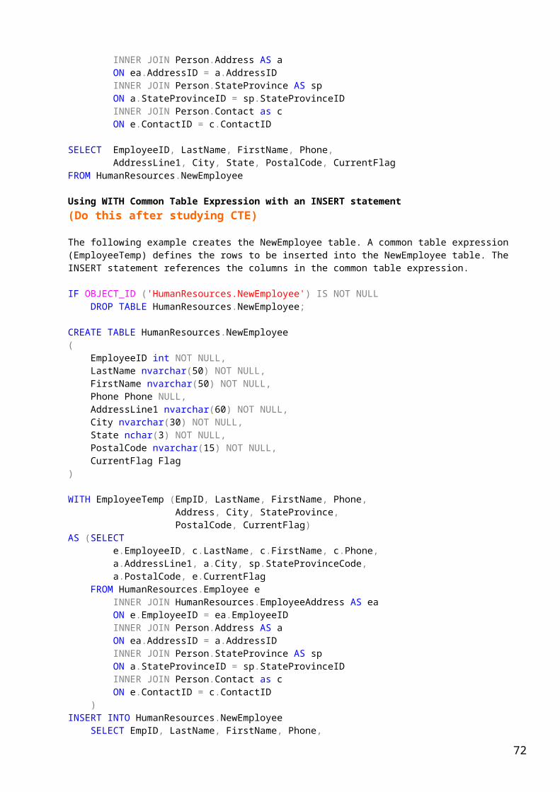
SELECT NumberEmployees, NULLIF(NumberEmployees, 10) AS manipulated_number_of_employees FROM dbo.DimReseller WHERE NumberEmployees IN (10, 11)

ISNULL:

The ISNULL accepts only two parameters. The first parameter will be checked, and if NULL value is found, it will be replaced with the second parameter. Furthermore, ISNULL requires that both parameters have the same data type.

Syntax:ISNULL ( check_expression , replacement_value )

Note:The value of check_expression is returned if it is not NULL; otherwise, replacement_value is returned after it is implicitly converted to the type of check_expression, if the types are different.

The following example finds the average of the weight of all products. It substitutes the value 50 for all NULL entries in the Weight column of the Product table.

SELECT AVG(ISNULL(Weight, 50))FROM Production.Product

One more example:The following example selects the description, discount percentage, minimum quantity, and maximum quantity for all special offers in AdventureWorks. If the maximum quantity for a particular special offer is NULL, the MaxQty shown in the result set is 0.00.

SELECT Description, DiscountPct, MinQty, ISNULL(MaxQty, 0.00) AS 'Max Quantity'FROM Sales.SpecialOffer

CAST and CONVERT Function:

The CAST and CONVERT functions are very similar: Both translate a value from one data type to another explicitly if parameter is compatible. The term compatible means ‘ABCD’ cannot be converted into 1234 and ‘1234’ can be converted into 1234. Although their performance is also similar, their syntax and potential usage is slightly different.

The syntax is as follows:

Syntax for CAST:CAST ( expression AS data_type [ (length ) ])

Syntax for CONVERT:CONVERT ( data_type [ ( length ) ] , expression [ , style ] )

Note: The style parameter is required only for date data type. This is an integer value from 1 to 130 for different style of date.

Example:

Pull HireDate from Employee table without Cast and convert Function.

select HireDate from HumanResources.Employee Result: 1996-07-31 00:00:00.000

select Cast(HireDate as varchar (12)) from HumanResources.Employee

72

Result: Jul 31 1996

The convert function without style parameter gives output with same format as of Cast function.

select Convert(varchar (12), HireDate) from HumanResources.Employee

Result: Jul 31 1996

The convert function with style parameter:

select Convert(varchar (12), HireDate,110) from HumanResources.Employee

Result: 07-31-1996

Note: You can try with 1 to 130 numbers for style parameter for different styles of date value.

Usages of Cast & Convert function with numeric data type:

This example converts ListPrice from Float to Int Data type:

SELECT SUBSTRING(Name, 1, 30) AS ProductName, ListPrice, CAST(ListPrice AS int) as ListPrice_IntFROM Production.ProductWHERE ListPrice > 0

ProductName ListPrice ListPrice_Int======================= ========= =============LL Mountain Seat Assembly 133.34 133ML Mountain Seat Assembly 147.14 147HL Mountain Seat Assembly 196.92 197LL Road Seat Assembly 133.34 133ML Road Seat Assembly 147.14 147HL Road Seat Assembly 196.92 197

SELECT SUBSTRING(Name, 1, 30) AS ProductName, ListPrice, CONVERT(int, ListPrice) as ListPrice_IntFROM Production.ProductWHERE ListPrice>0

Output: Same as of Cast Function

Try the following examples to see the impact of functions

SELECT SalesYTD/CommissionPCT AS 'Computed'FROM Sales.SalesPerson WHERE CommissionPCT != 0;

Output: 379753753.825

SELECT ROUND(SalesYTD/CommissionPCT, 2) AS 'Computed'FROM Sales.SalesPerson WHERE CommissionPCT != 0;

Output: 379753753.83

SELECT CAST(ROUND(SalesYTD/CommissionPCT, 2) AS int) AS 'Computed'FROM Sales.SalesPerson WHERE CommissionPCT != 0;

Output: 379753754

Using CAST to concatenate:

73

SELECT 'The list price is ' + CAST(ListPrice AS varchar(12)) AS ListPriceFROM Production.ProductWHERE ListPrice BETWEEN 350.00 AND 400.00

Output:ListPric==========================The list price is 357.06The list price is 364.09The list price is 364.09The list price is 364.09The list price is 364.09

Using CAST to produce more readable text:

Compare the output of both queries:

SELECT DISTINCT p.Name, s.UnitPriceFROM Sales.SalesOrderDetail s JOIN Production.Product p on s.ProductID = p.ProductIDWHERE Name LIKE 'Long-Sleeve Logo Jersey, M';

Name UnitPrice========================== ========Long-Sleeve Logo Jersey, M 27.4945Long-Sleeve Logo Jersey, M 27.879Long-Sleeve Logo Jersey, M 28.8404Long-Sleeve Logo Jersey, M 28.9942

SELECT DISTINCT CAST(p.Name AS char(10)) AS Name, s.UnitPriceFROM Sales.SalesOrderDetail s JOIN Production.Product p on s.ProductID = p.ProductIDWHERE Name LIKE 'Long-Sleeve Logo Jersey, M';

Name UnitPrice========================== ========Long-Sleev 27.4945Long-Sleev 27.879Long-Sleev 28.8404Using CAST with the LIKE clause:

The following example converts the money column SalesYTD to an int and then to a char(20) column so that it can be used with the LIKE clause.

SELECT p.FirstName, p.LastName, s.SalesYTD, s.SalesPersonIDFROM Person.Contact p JOIN Sales.SalesPerson s ON p.ContactID = s.SalesPersonIDWHERE CAST(CAST(s.SalesYTD AS int) AS char(20)) LIKE '2%';

FirstName LastName SalesYTD SalesPersonID========= ======== ======== =============Carol Elliott 2811012.7151 279Julie Estes 219088.8836 288Janeth Esteves 2241204.0424 289

ISDATE Function:

This function determines whether an input expression is a valid date. And returns 1 if the input expression is a valid date; otherwise, it returns 0.

DECLARE @datestring varchar(8)SET @datestring = '12/21/1998'SELECT ISDATE(@datestring)

74

Result=====1

One more Example:

SELECT ISDATE('february 31, 2009') AS 'february 39, 2009', ISDATE('february 25, 2009') AS 'february 25, 2009', ISDATE('January 1, 2009') AS '1/1/2009'

february 39, 2009 february 25, 2009 1/1/2009================== ================= =========0 1 1

ISNUMERIC Function:

The ISNUMERIC deterministic function determines whether the parameter passed is of a numeric data type. This function returns a BIT value, as in the following example:

SELECT ISNUMERIC('abc') AS 'abc', ISNUMERIC('123.45') AS '123.45'

Output: 0 1

CURRENT_TIMESTAMP Function:The CURRENT_TIMESTAMP function works exactly the same way as GETDATE: It returns current date and time. For example:

SELECT CURRENT_TIMESTAMP

select Getdate()

Same output of both functions: 2010-01-23 15:38:21.403

DATALENGTH Function:

This function is returns same output as of Len function to return the length of a value stored in a column:

Example:

select Len('Rabi Lal Puri') as Name_Lenth, DATALENGTH('Rabi Lal Puri') AS Name_Lenth2

Output:Name_Lenth Name_Lenth2=========== ===========13 13

ERROR_MESSAGE Function:

The ERROR_MESSAGE function returns the text of the error which caused the CATCH block of TRY / CATCH logic to execute. This function can be very useful in determining the statement that caused the error and troubleshooting the code module (stored procedure) that encountered the error. The function does not accept any parameters. For example, the following query returns the error text:

First try this query:

SELECT 1 / 0 as Divison

Output:

75

Msg 8134, Level 16, State 1, Line 1Divide by zero error encountered.

Now Try the following query:

BEGIN TRY

SELECT 1 / 0 as Divison END TRY BEGIN CATCH

SELECT 'the error was: ' + ERROR_MESSAGE() as [Divison by Zero]END CATCH

ERROR_NUMBER Function:

The ERROR_NUMBER function returns the number of the error which caused the CATCH block of TRY / CATCH logic to execute. This function can be very useful in determining the statement that caused the error and troubleshooting the code module (stored procedure) that encountered the error. The function does not accept any parameters. For example, the following query returns the error number:

BEGIN TRY

SELECT 1 / 0 END TRY BEGIN CATCH

SELECT 'the error number was: ' + CAST(ERROR_NUMBER() AS VARCHAR) END CATCH

ERROR_PROCEDURE Function:

The ERROR_PROCEDURE function returns the name of the stored procedure or trigger that encountered the error. This function does not accept any parameters and can be effectively called from CATCH block. For example, the following query creates a stored procedure that intentionally causes divide by zero error. Next the procedure is executed and the name of the erroneous stored procedure is returned:

Create the following procedure:

CREATE PROCEDURE my_test_proc AS SELECT 1 / 0

Execute the procedure:

EXEC my_test_proc

See the output:

Msg 8134, Level 16, State 1, Procedure my_test_proc, Line 2Divide by zero error encountered.

To find where the error occurred, run the procedure between try and catch block and see the error:

BEGIN TRY EXEC my_test_proc END TRY BEGIN CATCH SELECT 'the erroneous procedure was: ' + ERROR_PROCEDURE() END CATCH

Output:

the erroneous procedure was: my_test_proc

76

ERROR_SEVERITY Function:

The ERROR_SEVERITY function returns the severity of the error which caused the CATCH block of TRY / CATCH logic to execute. The function does not accept any parameters. For example, the following query returns the error severity:

BEGIN TRY SELECT 1 / 0 END TRY BEGIN CATCH SELECT 'the error severity was: ' + CAST(ERROR_SEVERITY() AS VARCHAR) END CATCH

Output:the error severity was: 16

Now Scalar functions are over. We have already done Aggregate Functions. Let’s begin SQL Server 2005 Ranking Functions.

Ranking Functions:

Ranking functions return a ranking value for each row in a partition. Depending on the function used, some rows might receive the same value as other rows.

Ranking functions are of 4 types:

ROW_NUMBER Function Rank Function Dense_Rank Function NTILE Function

Create the following table in your test database and insert the following data.

Create Table Person(FirstName varchar(25),Age int,Gender char(1))

FirstName Age Gender======== ==== ======Doris 6 FMary 11 FSherry 11 FSue 29 FLarry 5 MGeorge 6 MSam 17 MTed 23 MRojy 23 F

Now implement the Ranking Functions with the data.

ROW_NUMBER Function:

This function returns a sequential number starting at 1 for each row or grouping within your result set.

Syntax:

ROW_NUMBER ( ) OVER ( [ <partition_by_clause> ] <order_by_clause> )

Where the:

<partition_by_clause>

77

is a column or set of columns used to determine the grouping in which the Row_Number function applies sequential numering. This is an optional clause.

<order_by_clause>:Is a column or a set of columns used to Rank the result set.

First run the query and see the table putput.select * from person

Now run the following query to assign the row number to the output:

Select Row_Number() over(Order by Age) as SN,FirstName, Agefrom Person

SN FirstName Age=== ======== ===1 Larry 52 George 63 Doris 64 Mary 115 Sherry 116 Sam 177 Ted 238 Rojy 239 Sue 29

Row_Number() function with partion clause sequentially numbers group of rows. The rows will be sequentially numbered within each unique partition value. The sequential number will start at 1 for each new partition value in record set.Example:Select Row_Number() over(Partition by gender Order by Age desc) as SN,FirstName, Age, Genderfrom Person

SN FirstName Age Gender=== ======== === ======1 Sue 29 F2 Rojy 23 F3 Mary 11 F4 Sherry 11 F1 Ted 23 M2 Sam 17 M3 George 6 M4 Larry 5 M

The output is partitioned by gender and ordered by Age.

Rank_Function:

Syntax:

RANK ( ) OVER ( [ < partition_by_clause > ] < order_by_clause > )

This function returns the rank of each row within the partition of a result set.Sometimes you want to have the same rank for the same value. For this Rank function is handy.

Example:

Select Rank() over(Order by Age) as SN,FirstName, Age, Genderfrom Person

output:SN FirstName Age Gender

78

=== ======== === ======1 Larry 5 M2 George 6 M2 Doris 6 F4 Mary 11 F4 Sherry 11 F6 Sam 17 M7 Ted 23 M7 Rojy 23 F9 Sue 29 F

Here, equal Age has the same rank.

Ranking with Partition:

Select Rank() over(Partition by gender Order by Age) as SN,FirstName, Age, Genderfrom Person

output:SN FirstName Age Gender=== ======== === ======

1 Doris 6 F2 Mary 11 F2 Sherry 11 F4 Rojy 23 F5 Sue 29 F1 Larry 5 M2 George 6 M3 Sam 17 M4 Ted 23 M

Here you can see that the “F” Gender started ranking at 1 and goes through 5, then the ranking starts over with 1 when the first “M” Gender is encountered.

Dense_Rank Function:

Returns the rank of rows within the partition of a result set, without any gaps in the ranking. The rank of a row is one plus the number of distinct ranks that come before the row in question.

DENSE_RANK ( ) OVER ( [ < partition_by_clause > ] < order_by_clause > )

Select Dense_Rank() over(Order by Age) as SN,FirstName, Age, Genderfrom Person

SN FirstName Age Gender=== ======== === ======1 Doris 6 F2 Mary 11 F2 Sherry 11 F3 Rojy 23 F4 Sue 29 F1 Larry 5 M2 George 6 M3 Sam 17 M4 Ted 23 M

Dense_Rank is same as Rank except it does not leave gap in ranking.

In Rank function the was like 1 2 2 4. With Dense_Rank, the ranking is like 1 2 2 3.

Dense_Rank Function with Partition clause:

79

Select Dense_Rank() over(Partition by gender Order by Age) as SN,FirstName, Age, Genderfrom Person

SN FirstName Age Gender=== ======== === ======1 Doris 6 F2 Mary 11 F2 Sherry 11 F3 Rojy 23 F4 Sue 29 F1 Larry 5 M2 George 6 M3 Sam 17 M4 Ted 23 M

NTILE Function:

Syntax:NTILE (integer_expression)OVER ( [ <partition_by_clause> ] < order_by_clause > )Distributes the rows in an ordered partition into a specified number of groups. The groups are numbered, starting at one. For each row, NTILE returns the number of the group to which the row belongs.

Select NTILE(2) over(Order by Age) as SN,FirstName, Age, Genderfrom Person

SN FirstName Age Gender=== ======== === ======1 Larry 5 M1 George 6 M1 Doris 6 F1 Mary 11 F1 Sherry 11 F2 Sam 17 M2 Ted 23 M2 Rojy 23 F2 Sue 29 F

NTILE Function with Partition clause:

Select NTILE(2) over(Partition by gender Order by Age) as SN,FirstName, Age, Genderfrom Person

SN FirstName Age Gender=== ========= === ======1 Doris 6 F1 Mary 11 F1 Sherry 11 F2 Rojy 23 F2 Sue 29 F1 Larry 5 M1 George 6 M2 Sam 17 M2 Ted 23 M

Some Examples from books:

ROW_NUMBER:

SELECT ROW_NUMBER() OVER(ORDER BY SalesYTD DESC) AS 'Row Number',c.FirstName, c.LastName, s.SalesYTD, a.PostalCode

80

FROM Sales.SalesPerson s JOIN Person.Contact c on s.SalesPersonID = c.ContactIDJOIN Person.Address a ON a.AddressID = c.ContactIDWHERE TerritoryID IS NOT NULL AND SalesYTD <> 0

Can we limit the rows using row number generated by Row_BUMBER function?

Solution: Use CTE

WITH OrderedOrders AS(SELECT SalesOrderID, Convert(varchar (12), OrderDate,110) as OrdDate,ROW_NUMBER() OVER (order by OrderDate)as RowNumberFROM Sales.SalesOrderHeader ) SELECT * FROM OrderedOrders WHERE RowNumber between 50 and 60

SalesOrderId OrdDate RowNumber43708 07-03-2001 5043709 07-03-2001 5143710 07-03-2001 5243711 07-04-2001 5343712 07-04-2001 5443713 07-05-2001 5543714 07-05-2001 5643715 07-05-2001 57NOTE:

To understand the ranking functions, keep two things in mind: Partition clause is used to divide the rows in groups with unique value of

the specified column in partition clause Order by clause is used to generate the sequential number based on the

value (descending or ascending).

System defined Stored Procedures:

To see all tables and views in the current database:For same results:EXEC sp_tables

select * from information_schema.tables

sp_rename

This procedure changes the name of a user-created object in the current database.

Syntax and Example:

EXEC sp_rename Old_Object, New_Object

EXEC sp_rename 'Sales.SalesTerritory', 'SalesTerr'

To check what columns are defined in a data dictionary for a user defined table?EXEC sp_columns 'Sales'

To displays the definition of a user-defined rule, default, unencrypted Transact-SQL stored procedure, user-defined Transact-SQL function, trigger, computed column, CHECK constraint, view, or system object such as a system stored procedure.

EXEC sp_helptext 'sp_helpfile'EXEC sp_helptext View1EXEC sp_helptext 'Order Details Extended' -- for procedure

81

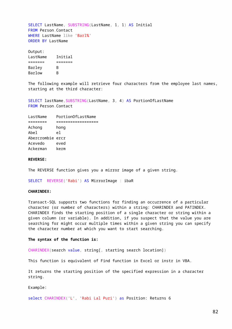
Find out which stored procedures are in a database:

EXEC sp_stored_procedures

If the database db1 was marked suspect during recovery due to insufficient space (error 1105) in file group fg1.

USE master;GOEXEC sp_add_data_file_recover_suspect_db db1, fg1, file2,'C:\Program Files\Microsoft SQL Server\MSSQL.1\MSSQL\Data\db1_file2.mdf', '1MB'

This command adds a data file to a filegroup when recovery cannot complete on a database due to insufficient space on the file group (error 1105). After the file is added, this stored procedure turns off the suspect setting and completes the recovery of the database.

To find all information about a database object (any object listed in the sys.sysobjects compatibility view), a user-defined data type, or a data type.

sp_help

To return a list of all constraint types, their user-defined or system-supplied name, the columns on which they have been defined in a Table:

EXEC sp_helpconstraint 'Production.Product'

To get all information about a specified database or all databases in a server:

sp_helpdb

Returns the physical names and attributes of files associated with the current database. Use this stored procedure to determine the names of files to attach to or detach from the server.

sp_helpfile

Returns the names and attributes of filegroups associated with the current database.

sp_helpfilegroup

To get all information about the indexes on a particular table or a view:

EXEC sp_helpindex 'Sales.Customer'

To know what human languages are supported by SQL Server?

sp_helplanguage

To display server name and other information like the network name of the server, the replication status of the server, the identification number of the server and the collation name.

sp_helpserverTo know the type or types of DML triggers defined on the specified table for the current database. sp_helptrigger cannot be used with DDL triggers. Query the sys.triggers (Transact-SQL) catalog view to for DDL Trigger.

EXEC sp_helptrigger 'Person.Contact'

To get information about locks:

82

sp_lock

OR

select * from sys.dm_tran_locks

To displays statistics about Microsoft SQL Server:

sp_monitor

To cause stored procedures and triggers to be recompiled the next time they are run:Syntax: EXEC sp_recompile ‘Table_Name’

Example:EXEC sp_recompile 'Sales.Customer'

Output Message:

Object 'Sales.Customer' was successfully marked for recompilation.

It means any trigger or procedures based on the customer table will be automatically recompiled if the table gets any changes.

To changes the name of a database:

sp_renamedb 'old_name' , 'new_name'

For Example:

USE masterGOCREATE DATABASE AccountingGOEXEC sp_renamedb 'Accounting', 'Financial'GOSELECT name, database_id, modified_dateFROM sys.databasesWHERE name = 'Financial'

To display the number of rows, disk space reserved, and disk space used by a table, indexed view or displays the disk space reserved and used by the whole database:

EXEC sp_spaceused -- Space used by whole databaseEXEC sp_spaceused 'Purchasing.Vendor' --Space used by an object like table

To get information about current users and processes in an instance of the Microsoft SQL Server Database Engine:

sp_who

Data Integrity:

The data integrity refers to the accuracy, consistency and correctness of data.Enforcing data integrity guarantees the quality of the data in the database. For example, if an employee is entered with an employee_id value of 123, the database should not permit another employee to have an ID with the same value.

Types of data integrity: Entity Integrity Domain Integrity

83

Referential Integrity User-Defined Integrity

Entity Integrity:

Entity integrity defines a row as a unique entity for a particular table. Entity integrity enforces the integrity of the identifier columns or the primary key of a table, through indexes, UNIQUE constraints, PRIMARY KEY constraints, or IDENTITY properties.

Domain Integrity:

A domain is the set of all allowed values in a column.Domain integrity is the validity of entries for a specific column. You can enforce domain integrity to restrict the type by using data types, restrict the format by using CHECK constraints and rules, or restrict the range of possible values by using FOREIGN KEY constraints, CHECK constraints, DEFAULT definitions, NOT NULL definitions, and rules.

Referential Integrity:

Referential integrity preserves the defined relationships between tables when records are entered or deleted. In SQL Server 2005, referential integrity is based on relationships between foreign keys and primary keys or between foreign keys and unique keys. Referential integrity makes sure that key values are consistent across tables. This kind of consistency requires that there are no references to nonexistent values and that if a key value changes, all references to it change consistently throughout the database.

When you enforce referential integrity, SQL Server prevents users from doing the following:

Adding or changing records to a related table if there is no associated record in the primary table.

Changing values in a primary table that causes orphaned records in a related table.

Deleting records from a primary table if there are matching related records.

For example, with the Sales.SalesOrderDetail and Production.Product tables in the AdventureWorks database, referential integrity is based on the relationship between the foreign key (ProductID) in the Sales.SalesOrderDetail table and the primary key (ProductID) in the Production.Product table. This relationship makes sure that a sales order can never reference a product that does not exist in the Production.Product table.

84

User-Defined Integrity:

User-defined integrity lets you define specific business rules that do not fall into one of the other integrity categories. All the integrity categories support user-defined integrity. This includes all column-level and table-level constraints in CREATE TABLE, stored procedures, and triggers.

Constraints:

Constraints define rules regarding the values allowed in columns and are the standard mechanism for enforcing integrity. Using constraints is preferred to using DML Triggers, rules, and defaults.Types of constraints:

PRIMARY KEY Constraints UNIQUE Constraints FOREIGN KEY Constraints CHECK Constraints DEFAULT Definitions Allowing Null Values

PRIMARY KEY Constraints:

A table typically has a column or combination of columns that contain values that uniquely identify each row in the table. This column, or columns, is called the primary key (PK) of the table and enforces the entity integrity of the table. You can create a primary key by defining a PRIMARY KEY constraint when you create or modify a table.

A table can have only one PRIMARY KEY constraint, and a column that participates in the PRIMARY KEY constraint cannot accept null values. Because PRIMARY KEY constraints guarantee unique data, they are frequently defined on an identity column.

When you specify a PRIMARY KEY constraint for a table, the SQL Server 2005 Database Engine enforces data uniqueness by creating a unique index for the primary key columns. This index also permits fast access to data when the primary key is used in queries. Therefore, the primary keys that are chosen must follow the rules for creating unique indexes.

If a PRIMARY KEY constraint is defined on more than one column, values may be duplicated within one column, but each combination of values from all the columns in the PRIMARY KEY constraint definition must be unique.

The following example creates the part_sample table and specifies the part_nmbr field as the primary key.

CREATE TABLE part_sample(part_nmbr int PRIMARY KEY, part_name char(30), part_weight decimal(6,2), part_color char(15) )

How to create a composit PK?

Create table t1(A int not null, B Datetime not null, C varchar(10),Constraint PKC Primary Key(A,C))

85

This definition creates a table t1, unique clustered index with name ‘PKC’. Constraint Keys and Index Keys are (A, C) for both. Constraint name and Index name is same as PKC.

How to create PK constraint in existing table?We have the following table without PK Constraint:

Create table T1(A int not null, B Datetime not null, C varchar(10))

Now alter the table and add PK Constraint as:Syntax:

Alter Table Table_NameAdd Constraint Constraint_Name Constraint_Type (Field)

Example:

Alter table T1Add Constraint PKC Primary Key (A)

Import table from AdventureDB and add PK and FK constraints:

alter table HumanResources.Departmentadd constraint pk primary key (DepartmentID)

How to remove constraint if we don’t want it to be in a table?

Alter table T1Drop constraint PKC

UNIQUE Constraints:

You can use UNIQUE constraints to make sure that no duplicate values are entered in specific columns that do not participate in a primary key. Although both a UNIQUE constraint and a PRIMARY KEY constraint enforce uniqueness, use a UNIQUE constraint instead of a PRIMARY KEY constraint when you want to enforce the uniqueness of a column, or combination of columns, that is not the primary key.

Multiple UNIQUE constraints can be defined on a table, whereas only one PRIMARY KEY constraint can be defined on a table.

Also, unlike PRIMARY KEY constraints, UNIQUE constraints allow for the value NULL. However, as with any value participating in a UNIQUE constraint, only one null value is allowed per column.

A UNIQUE constraint can be referenced by a FOREIGN KEY constraint.

You can create a UNIQUE constraint as part of the table definition when you create a table. If a table already exists, you can add a UNIQUE constraint, provided that the column or combination of columns that make up the UNIQUE constraint contains only unique values. A table can contain multiple UNIQUE constraints.

You can create a UNIQUE constraint as part of the table definition when you create a table. If a table already exists, you can add a UNIQUE constraint, provided that the column or combination of columns that make up the UNIQUE constraint contains only unique values. A table can contain multiple UNIQUE constraints.

When a UNIQUE constraint is added to an existing column or columns in the table, by default, the SQL Server 2005 Database Engine examines the existing data in the

86

columns to make sure all values are unique. If a UNIQUE constraint is added to a column that has duplicated values, the Database Engine returns an error and does not add the constraint.

The Database Engine automatically creates a UNIQUE index to enforce the uniqueness requirement of the UNIQUE constraint. Therefore, if an attempt to insert a duplicate row is made, the Database Engine returns an error message that states the UNIQUE constraint has been violated and does not add the row to the table. Unless a clustered index is explicitly specified, a unique, nonclustered index is created by default to enforce the UNIQUE constraint.

To remove the uniqueness requirement for values entered in the column or combination of columns included in the constraint, delete a UNIQUE constraint. You cannot delete a UNIQUE constraint if the associated column is used as the full-text key of the table.

Create a unique constraint:

Create Table Emp( EmpId smallint not null identity(1000,1), SSN char(9) not null, Fname varchar(20), DOB SmallDatetime, salary money, Constraint PKC_N Primary key (EmpId Asc), --PK Constraint Constraint UC Unique (SSN Asc)) --Unique Constraint

Add unique constraint in an existing table:

Alter table EmpAdd constraint UC Unique constraint (SSN Asc)

FOREIGN KEY Constraints:

A foreign key (FK) is a column or combination of columns that is used to establish and enforce a link between the data in two tables. You can create a foreign key by defining a FOREIGN KEY constraint when you create or modify a table.

In a foreign key reference, a link is created between two tables when the column or columns that hold the primary key value for one table are referenced by the column or columns in another table. This column becomes a foreign key in the second table.

This constraint enforces referential integrity by guaranteeing that changes cannot be made to data in the primary key table if those changes invalidate the link to data in the foreign key table. If an attempt is made to delete the row in a primary key table or to change a primary key value, the action will fail when the deleted or changed primary key value corresponds to a value in the FOREIGN KEY constraint of another table. To successfully change or delete a row in a FOREIGN KEY constraint, you must first either delete the foreign key data in the foreign key table or change the foreign key data in the foreign key table, which links the foreign key to different primary key data.

Number of FOREIGN KEY Constraints in a Table:

SQL Server does not have a predefined limit for the number of FOREIGN KEY constraints a table can contain. However, SQL Server recommends that a table contains no more than 253 FOREIGN KEY constraints.

Example of Creating FOREIGN KEY ConstraintsCREATE TABLE order_part (order_nmbr int,

87

part_nmbr int FOREIGN KEY REFERENCES part_sample(part_nmbr), qty_ordered int)

Note:

We know we cannot update or delete rows in a parent table if it has a child table with matching key value. If we need to do so, we must use cascade Actions. If cascade actions are defined, all rows with matching values are first deleted or changed in the child table before those rows can be deleted or changed in the parent table.

Cascade or Referential actions are of 4 types: No Action Cascade Set Null Set Default

No Action:It is default action. The referential integrity is strictly enforced so that an error is raised if the parent row is deleted or updated if there is a matching value in the FK column in the child table.

Cascade:

If this action is defined, the database engine automatically deletes or updates all rows in the child table with the matching foreign key values which corresponds to the rows affected in the parent table.

Set Null:

If this action is defined, the database engine automatically sets all of the matching foreign key values in the child table to Null.

Set Default:

The database engine automatically sets the entire matching foreign key values in the child table to the default value to the column. The default value has to be defined while creating FK constraint. If default is not defined and the column is NULLable, Null would be assigned as default value. Unlike a primary key constraint, foreign key constraint is not automatically indexed by the database engine, so foreign key column has to be explicitly indexed.

Example of Foreign key constraint(Cascading Referential Integrity Constraints)

Suppose you have a master table Dept with PK (DeptId)Now create a child table EMP as …….. Create Table EMP( EmpId int Not Null Identity (1000,1),

. . .,

. . .,

. . .,

. . .,

. . .,Constraint PK_Emp_Id Primary key (EmpId),Constraint FK_Dept_Id Foreign key (DeptID)References Dept(DeptID)ON Delete CascadeON Update Cascade

)-------------------All Referential Actions-----------------------[ ON DELETE { NO ACTION | CASCADE | SET NULL | SET DEFAULT } ]

88

[ ON UPDATE { NO ACTION | CASCADE | SET NULL | SET DEFAULT } ]

How to define Cascading Referential Integrity Constraints in existing table?

Import table in your test database and do the following:

Alter Table HumanResources.Employee With NOCHECKadd constraint FK Foreign key (DepartmentID) References HumanResources.Department(DepartmentID)ON Delete cascadeON Update cascade

Now Update master table and see the impact on chield table. You will see FK departmentId changed to 1000 which was 1 before update.

update HumanResources.Departmentset DepartmentId=1000 where DepartmentId=1What does the term ‘With NOCHECK’?

When we create a FK constraint in an existing table, by default the SQL Server database engine will validate the data in the foreign key when the constraint will be created. We can bypass the checking ‘With NOCHECK’ option in the alter command. It allows the existing rows to remain intact that do not meet the criteria of KK. There after added or deleted will be validated against the constraint.

CHECK Constraints:

CHECK constraints enforce domain integrity by limiting the values that are accepted by a column. CHECK constraints determine the valid values from a logical expression.

You can create a CHECK constraint with any logical (Boolean) expression that returns TRUE or FALSE based on the logical operators, List operator, Range operator, comparison operators and pattern match (Like). For example, the logical expression is: salary >= 15000 AND salary <= 100000.

You can create a CHECK constraint as part of the table definition when you create a table. If a table already exists, you can add a CHECK constraint

Use the WITH NOCHECK option of the ALTER TABLE statement to apply the new constraint only to newly added data. This option is useful when the existing data already meets the new CHECK constraint, or when a business rule requires the constraint to be enforced only from this point forward.

Note: To modify a CHECK constraint, you must first delete the existing CHECK constraint and then re-create it with the new definition.Check constraint is valideted only the time of insert and update, not for delete.

Example to create Check Constraint:

Create table Emp( -,

-,-,Salary money,Constraint CH_Sal Check (Salary > 0 and Salary <= 500)

)

If your table exits, you can add it altering the table.

Alter Table Emp Add Constraint CH_Salary CHECK (Salary > 0 and Salary <= 500)

89

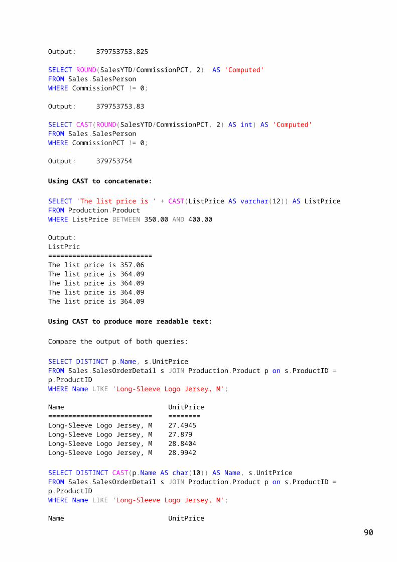
Some examples of Check constraint:

IN:Alter Table Emp Add Constraint CH_City CHECK (City IN (‘Delhi’,’Chandigarh’,’...’,’...’))

LIKE:Alter Table Emp Add Constraint CH_PIN CHECK (PIN LIKE "[0-9][0-9][0-9][0-9][0-9][0-9]")

Between:Alter Table Emp Add Constraint CH_BTN CHECK (TotalAmt Between 1000 And 5000)

The following example disables a constraint that limits the salaries accepted in the data. NOCHECK CONSTRAINT is used with ALTER TABLE to disable the constraint and allow for an insert that would typically violate the constraint. CHECK CONSTRAINT reenables the constraint.

Enabling or Disabling Constraints:

Only FK Constraint and Check Constraint are enabled and disabled.Syntax is same for both constraints.

Disabale FK / Check constraints:

Alter Table TableNameNOCHECK CONSTRAINT CONSTRAINT_NAME

Enabale FK / Check constraints:

Alter Table TableNameCHECK CONSTRAINT CONSTRAINT_NAME

CREATE TABLE CH_Constraint (id INT NOT NULL, FName VARCHAR(10) NOT NULL, salary MONEY NOT NULL CONSTRAINT salary_cap CHECK (salary < 100000))

-- Valid insertsINSERT INTO CH_Constraint VALUES (1,'Rajwant',65000)INSERT INTO CH_Constraint VALUES (2,'Ram',75000)

-- This insert violates the constraint.INSERT INTO CH_Constraint VALUES (3,'Hari',105000)

-- Disable the constraint and try again.ALTER TABLE CH_Constraint NOCHECK CONSTRAINT salary_cap

INSERT INTO CH_Constraint VALUES (3,'Suraj',105000)

-- Re-enable the constraint and try another insert; this will fail.ALTER TABLE CH_Constraint CHECK CONSTRAINT salary_cap

INSERT INTO CH_Constraint VALUES (4,'Rosan',110000)

DEFAULT Definitions:

90

A default definition provides automatic entry of a default value for a column when an insert statement does not specify the value for that column. The default constraint enforces domain integrity assigning a constant value to a column.

The default constraint can be applied with any column except identity property and timestamp column.

The detault constraint is applicable only to insert statement.

Example of default constraint:

Create table Emp( -,

-,-,City varchar(20) NOT NULL Default 'Delhi',

)

OR

Alter Table EMPAdd Constraint Def_CT Default 'Delhi' For City

To modify a DEFAULT definition, you must first drop the existing DEFAULT definition and then re-create it with the new definition.

Limitations of all constraints:

PRIMARY KEY ConstraintsA table can contain only one PRIMARY KEY constraint.

The index generated by a PRIMARY KEY constraint cannot cause the number of indexes on the table to exceed 249 nonclustered indexes and 1 clustered index.

If CLUSTERED or NONCLUSTERED is not specified for a PRIMARY KEY constraint, CLUSTERED is used if there are no clustered indexes specified for UNIQUE constraints.

All columns defined within a PRIMARY KEY constraint must be defined as NOT NULL. If nullability is not specified, all columns participating in a PRIMARY KEY constraint have their nullability set to NOT NULL.

UNIQUE ConstraintsIf CLUSTERED or NONCLUSTERED is not specified for a UNIQUE constraint, NONCLUSTERED is used by default.

Each UNIQUE constraint generates an index. The number of UNIQUE constraints cannot cause the number of indexes on the table to exceed 249 nonclustered indexes and 1 clustered index.

FOREIGN KEY ConstraintsWhen a value other than NULL is entered into the column of a FOREIGN KEY constraint, the value must exist in the referenced column; otherwise, a foreign key violation error message is returned.

FOREIGN KEY constraints are applied to the preceding column, unless source columns are specified.

FOREIGN KEY constraints can reference only tables within the same database on the same server. Cross-database referential integrity must be implemented through triggers.

FOREIGN KEY constraints can reference another column in the same table. This is referred to as a self-reference.

91

The REFERENCES clause of a column-level FOREIGN KEY constraint can list only one reference column. This column must have the same data type as the column on which the constraint is defined.

The REFERENCES clause of a table-level FOREIGN KEY constraint must have the same number of reference columns as the number of columns in the constraint column list. The data type of each reference column must also be the same as the corresponding column in the column list.

CASCADE, SET NULL or SET DEFAULT cannot be specified if a column of type timestamp is part of either the foreign key or the referenced key.

CASCADE, SET NULL, SET DEFAULT and NO ACTION can be combined on tables that have referential relationships with each other. If the Database Engine encounters NO ACTION, it stops and rolls back related CASCADE, SET NULL and SET DEFAULT actions. When a DELETE statement causes a combination of CASCADE, SET NULL, SET DEFAULT and NO ACTION actions, all the CASCADE, SET NULL and SET DEFAULT actions are applied before the Database Engine checks for any NO ACTION.

The Database Engine does not have a predefined limit on either the number of FOREIGN KEY constraints a table can contain that reference other tables, or the number of FOREIGN KEY constraints that are owned by other tables that reference a specific table. FOREIGN KEY constraints are not enforced on temporary tables.

FOREIGN KEY constraints can reference only columns in PRIMARY KEY or UNIQUE constraints in the referenced table or in a UNIQUE INDEX on the referenced table.

If a foreign key is defined on a CLR user-defined type column, the implementation of the type must support binary ordering. For more information, see CLR User-Defined Types.

A column of type varchar(max) can participate in a FOREIGN KEY constraint only if the primary key it references is also defined as type varchar(max).

DEFAULT DefinitionsA column can have only one DEFAULT definition.

A DEFAULT definition can contain constant values, functions or NULL.

Constant expression in a DEFAULT definition cannot refer to another column in the table, or to other tables, views, or stored procedures.

DEFAULT definitions cannot be created on columns with a timestamp data type or columns with an IDENTITY property.

DEFAULT definitions cannot be created for columns with alias data types if the alias data type is bound to a default object.

CHECK ConstraintsA column can have any number of CHECK constraints, and the condition can include multiple logical expressions combined with AND and OR. Multiple CHECK constraints for a column are validated in the order they are created.

The search condition must evaluate to a Boolean expression and cannot reference another table.

A column-level CHECK constraint can reference only the constrained column, and a table-level CHECK constraint can reference only columns in the same table.

CHECK CONSTRAINTS and rules serve the same function of validating the data during INSERT and UPDATE statements.

92

When a rule and one or more CHECK constraints exist for a column or columns, all restrictions are evaluated.

CHECK constraints cannot be defined on text, ntext, or image columns.

Additional Constraint InformationAn index created for a constraint cannot be dropped by using DROP INDEX; the constraint must be dropped by using ALTER TABLE. An index created for and used by a constraint can be rebuilt by using DBCC DBREINDEX.

Constraint names must follow the rules for identifiers, except that the name cannot start with a number sign (#). If constraint_name is not supplied, a system-generated name is assigned to the constraint. The constraint name appears in any error message about constraint violations.When a constraint is violated in an INSERT, UPDATE, or DELETE statement, the statement is ended. However, when SET XACT_ABORT is set to OFF, the transaction, if the statement is part of an explicit transaction, continues to be processed. When SET XACT_ABORT is set to ON, the whole transaction is rolled back. You can also use the ROLLBACK TRANSACTION statement with the transaction definition by checking the @@ERROR system function.

When ALLOW_ROW_LOCKS = ON and ALLOW_PAGE_LOCK = ON, row-, page-, and table-level locks are allowed when you access the index. The Database Engine chooses the appropriate lock and can escalate the lock from a row or page lock to a table lock. For more information, see Lock Escalation (Database Engine). When ALLOW_ROW_LOCKS = OFF and ALLOW_PAGE_LOCK = OFF, only a table-level lock is allowed when you access the index. For more information about configuring the locking granularity for an index, see Customizing Locking for an Index.

If a table has FOREIGN KEY or CHECK CONSTRAINTS and triggers, the constraint conditions are evaluated before the trigger is executed.

Crosstab queries using PIVOT in SQL Server 2005

Create the following table in your Sample table:create table Prd(SalesPerson varchar (20),Product varchar (20),SalesAmount money)

Insert the following data

SalesPerson Product SalesAmount=========== ======= ===========Rabi Pickles 100.00Hari Oranges 50.00Rajwant Pickles 25.00Rabi Pickles 75.00Rabi Oranges 80.00Hari Oranges 250.00Ram Pickles 100.00Rajwant Pickles 150.00Rajwant Oranges 160.00Hari Oranges 350.00Ram Oranges 180.00Hari Pickles 150.00Rajwant Oranges 160.00Hari Oranges 350.00Ram Oranges 180.00Hari Pickles 150.00

93

Now run the following query:

SELECT SalesPerson, [Oranges] AS Oranges, [Pickles] AS PicklesFROM (SELECT SalesPerson, Product, SalesAmount

FROM Prd ) psPIVOT(SUM (SalesAmount)FOR Product IN( [Oranges], [Pickles])) AS pvt

Output:SalesPerson Oranges Pickles=========== ======= ===========Hari 1000.00 300.00Rabi 80.00 175.00Rajwant 320.00 175.00Ram 360.00 100.00

How does this work?To use PIVOT you need to understand the data and how you want the data displayed. First you have the data rows, such as SalesPerson and the columns, such as the Products and then the values to display for each cross section.There are three pieces that need to be understood in order to construct the query.

(1) The SELECT statement

SELECT SalesPerson, [Oranges] AS Oranges, [Pickles] AS Pickles This portion of the query selects the three columns for the final result set (SalesPerson, Oranges, Pickles)

(2) The query that pulls the raw data to be prepared

(SELECT SalesPerson, Product, SalesAmount FROM ProductSales) ps This query pulls all the rows of data that we need to create the cross-tab results. The (ps) after the query is creating a temporary table of the results that can then be used to satisfy the query for step 1.

(3) The PIVOT expression

PIVOT (SUM (SalesAmount) FOR Product IN ( [Oranges], [Pickles]) ) AS pvt This query does the actual summarization and puts the results into a temporary table called pvt

Another key thing to notice in here is the use of the square brackets [ ] around the column names in both the SELECT in part (1) and the IN in part (3). These are key, because the pivot operation is treating the values in these columns as column names and this is how the breaking and grouping is done to display the data.

One more example

To determine the number of purchase orders placed by certain employees through pivot table, use the following query that provides this report, broken down by vendor in PurchaseOrderHeader table:

SELECT VendorID, [164] AS Emp1, [198] AS Emp2, [223] AS Emp3, [231] AS Emp4, [233] AS Emp5FROM (SELECT PurchaseOrderID, EmployeeID, VendorIDFROM Purchasing.PurchaseOrderHeader) pPIVOT(

94

COUNT (PurchaseOrderID)FOR EmployeeID IN( [164], [198], [223], [231], [233] )) AS pvtORDER BY VendorID

Can we create a table with computed field so that we insert value in base column and the computed column gets its value through calculating as defined?

Yes. Let’s see:

CREATE TABLE mytable ( low int, high int, myavg AS (low + high)/2 )

insert into mytable (low,high) values(5,10)insert into mytable (low,high) values(100,50)

select * from mytable

Low High MyAvg==== === ====5 10 7100 50 75

Index:

An index is a physical structure containing pointers to the data. Indexes are created in an existing table to locate rows more quickly and efficiently. It is possible to create an index on one or more columns of a table, and each index is given a name. The users cannot see the indexes, they are just used to speed up queries. Effective indexes are one of the best ways to improve performance in a database application. A table scan happens when there is no index available to help a query. In a table scan SQL Server examines every row in the table to satisfy the query results. Table scans are sometimes unavoidable, but on large tables, scans have a terrific impact on performance.

Or

An index is an database object associated with a table or view that speeds retrieval of rows from the table or view. An index contains keys built from one or more columns in the table or view. These keys are stored in a structure (B-tree) that enables SQL Server to find the row or rows associated with the key values quickly and efficiently.

Note:Indexes are automatically created when PRIMARY KEY and UNIQUE constraints are defined on table columns. For example, when you create a table and identify a particular column to be the primary key, the SQL Server 2005 Database Engine automatically creates a PRIMARY KEY constraint and index on that column.

How Indexes Are Used by the Query Optimizer?

Well-designed indexes can reduce disk I/O operations and consume fewer system resources therefore improving query performance. Indexes can be helpful for a variety of queries that contain SELECT, UPDATE, or DELETE statements. Consider the query SELECT Title, HireDate FROM HumanResources.Employee WHERE EmployeeID = 250 in the AdventureWorks database. When this query is executed, the query optimizer evaluates each available method for retrieving the data and selects the most efficient method. The method may be a table scan, or may be scanning one or more indexes if they exist.

95

When performing a table scan, the query optimizer reads all the rows in the table, and extracts the rows that meet the criteria of the query. A table scan generates many disk I/O operations and can be resource intensive. However, a table scan could be the most efficient method if, for example, the result set of the query is a high percentage of rows from the table.

When the query optimizer uses an index, it searches the index key columns, finds the storage location of the rows needed by the query and extracts the matching rows from that location. Generally, searching the index is much faster than searching the table because unlike a table, an index frequently contains very few columns per row and the rows are in sorted order.

Types of Index:

Clustered Nonclustered Unique Index with included columns Indexed views Full-text

Clustered:

Clustered indexes sort and store the data rows in the table or view based on their key values. These are the columns included in the index definition. There can be only one clustered index per table, because the data rows themselves can be sorted in only one order.

The only time the data rows in a table are stored in sorted order is when the table contains a clustered index. When a table has a clustered index, the table is called a clustered table. If a table has no clustered index, its data rows are stored in an unordered structure called a heap.

Index Architecture:

SQL Server stores data in 8KB pages inside the database files. Once you have created indexes, you will have index pages as well as data pages. The data pages contain the information that users have inserted in the tables. The index pages are used to store a list of all the indexed column (called key values) along with a pointer to the location of the records that contains the value in the inserted table.

Note:

Both clustered and nonclustered indexes can be unique. If the index is not unique, multiple row can share same index value.

A table without a clustered index is called a heap table. For a heap, a row locator is a pointer to the row. For a clustered table, the row locator is the clustered index key.

Clustered index architecture:

In SQL Server, indexes are organized as B-trees. Each page in an index B-tree is called an index node. The top node of the B-tree is called the root node. The bottom level of nodes in the index is called the leaf nodes. Any index levels between the root and the leaf nodes are collectively known as intermediate levels. In a clustered index, the leaf nodes contain the data pages of the underlying table. The root and leaf nodes contain index pages holding index rows. Each index row contains a key value and a pointer to either an intermediate level page in the B-tree, or a data row in the leaf level of the index. The pages in each level of the index are linked in a doubly-linked list.

96

Clustered indexes have one row in sys.partitions, with index_id = 1 for each partition used by the index. By default, a clustered index has a single partition. When a clustered index has multiple partitions, each partition has a B-tree structure that contains the data for that specific partition. For example, if a clustered index has four partitions, there are four B-tree structures; one in each partition.

Depending on the data types in the clustered index, each clustered index structure will have one or more allocation units in which to store and manage the data for a specific partition. At a minimum, each clustered index will have one IN_ROW_DATA allocation unit per partition. The clustered index will also have one LOB_DATA allocation unit per partition if it contains large object (LOB) columns. It will also have one ROW_OVERFLOW_DATA allocation unit per partition if it contains variable length columns that exceed the 8,060 byte row size limit. For more information about allocation units, see Table and Index Organization.

The pages in the data chain and the rows in them are ordered on the value of the clustered index key. All inserts are made at the point where the key value in the inserted row fits in the ordering sequence among existing rows

Previous / Next Pointers:For a clustered index, the root_page column in sys.system_internals_allocation_units points to the top of the clustered index for a specific partition. SQL Server moves down the index to find the row corresponding to a clustered index key. To find a range of keys, SQL Server moves through the index to find the starting key value in the range and then scans through the data pages using the previous or next pointers. To find the first page in the chain of data pages, SQL Server follows the leftmost pointers from the root node of the index.

As we know, clustered index physically rarranges the data that user insert in tables. At the top of the B-Tree structure, you find the root page which contains

97

The root index page contains the pointers to 3 intermediate level index pages

the information about the location of other pages down to the line called intermediate level pages. These intermediate pages contain yet more ley values that point other intermediate pages or data pages. The page at the very bottom of a clustered index is called leaf pages that contain the actual data in order.

Index key is a column of our table on which we create an index. So index key column contains the actual value of a table column. That index key value points to the data row matching the same value in both data column and index key column (the common column).

Nonclustered:

A nonclustered index can be defined on a table or view with a clustered index or on a heap. Each index row in the nonclustered index contains the nonclustered key value and a row locator. This locator points to the data row in the clustered index or heap having the key value. The rows in the index are stored in the order of the index key values, but the data rows are not guaranteed to be in any particular order unless a clustered index is created on the table.You can create multiple nonclustered indexes on a table or indexed view. Generally, nonclustered indexes should be designed to improve the performance of frequently used queries that are not covered by the clustered index.

Nonclustered index Structure:

Nonclustered indexes have the same B-tree structure as clustered indexes, except for the following significant differences:

The data rows of the underlying table are not sorted and stored in order based on their nonclustered keys.

The leaf layer of a nonclustered index is made up of index pages instead of data pages.

Nonclustered indexes can be defined on a table or view with a clustered index or a heap. Each index row in the nonclustered index contains the nonclustered key value and a row locator. This locator points to the data row in the clustered index or heap having the key value.

The row locators in nonclustered index rows are either a pointer to a row or are a clustered index key for a row, as described in the following:

If the table is a heap, which means it does not have a clustered index, the row locator is a pointer to the row. The pointer is built from the file identifier (ID), page number, and number of the row on the page. The whole pointer is known as a Row ID (RID).

If the table has a clustered index, or the index is on an indexed view, the row locator is the clustered index key for the row. If the clustered index is not a unique index, SQL Server 2005 makes any duplicate keys unique by adding an internally generated value called a uniqueifier. This four-byte value is not visible to users. It is only added when required to make the clustered key unique for use in nonclustered indexes. SQL Server retrieves the data row by searching the clustered index using the clustered index key stored in the leaf row of the nonclustered index.

Unique:A unique index ensures that the index key contains no duplicate values and therefore every row in the table or view is in some way unique. Both clustered and nonclustered indexes can be unique.

Index with included columns:A nonclustered index that is extended to include nonkey columns in addition to the key columns.

98

Using Included Columns to Avoid Size Limits:

You can include nonkey columns in a nonclustered index to avoid exceeding the current index size limitations of a maximum of 16 key columns and a maximum index key size of 900 bytes. The Database Engine does not consider nonkey columns when calculating the number of index key columns or index key size.

For example, assume that you want to index the following columns in the Document table in the AdventureWorks sample database:

Title nvarchar(50)

Revision nchar(5)

FileName nvarchar(400)

Because an nvarchar data type requires 2 bytes for each character, an index that contains these three columns would exceed the 900 byte size limitation by 10 bytes (455 * 2). By using the INCLUDE clause of the CREATE INDEX statement, the index key could be defined as (Title, Revision) and FileName defined as a nonkey column. In this way, the index key size would be 110 bytes (55 * 2), and the index would still contain all the required columns. The following statement creates such an index.

Example:

CREATE INDEX IX_Document_Title ON Production.Document (Title, Revision) INCLUDE (FileName)Note:Nonkey columns are defined in the INCLUDE clause of the CREATE INDEX statement.Nonkey columns can only be defined on nonclustered indexes on tables or indexed views.

Indexed views:

If we create an index on a view, the view is called an indexed view.An index on a view materializes (executes), the view and the result set is permanently stored in a unique clustered index in the same way a table with a clustered index is stored. Nonclustered indexes on the view can be added after the clustered index is created.

View:Views are also known as virtual tables because the result set returned by the view has the same general form as a table with columns and rows, and views can be referenced just like tables in SQL statements. The result set of a standard view is not stored permanently in the database. Every time a query references a standard view, SQL Server 2005 substitutes the definition of the view into the query internally until a modified query is formed that only references base tables. It then runs the resulting query as usual.

Features of index:

Indexes are created on one or more columns of any tables.

Indexes accelarate the queries that jion tables and perform filtering, grouping and sorting of data.

Indexes are used to inforce uniqueness of rows (through unique index). Indexes are useful only if majority of data is unique in indexed column. When we modify data of indexed column, the associated indexes are

automatically updated if index or data pages are not split. The clustered index should be created before nonclustered index because the

clustered index changes the order of rows and nonclustered index should be rebuild.

99

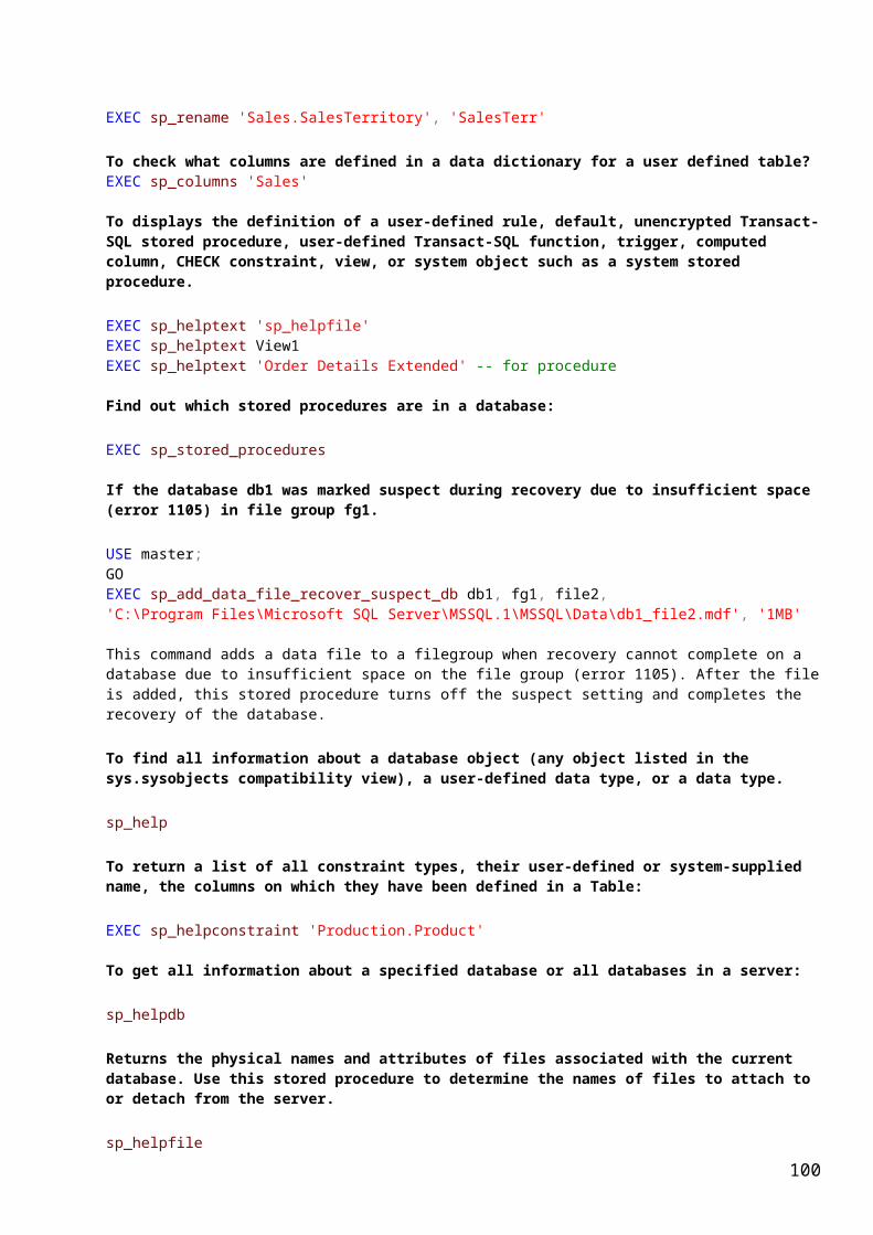
Guideline to create index:

Though we can create index on each column, it does not make any sense. We have to create index only on column which are used for filtering (where clause), join, grouping, PK, FK and the column which needs to be unique if it is not a PK.

Syntax to create index:

Create [UNIQUE][CLUSTERED|NONCLUSTERED] INDEX [Index_Name]ON SCHEMA.TABLE (COLUMN [,COLUMN].....)Include (COLUMN [,COLUMN].....)

Rebuilding Index:

The SQL Server Database Engine automatically maintains indexes whenever insert, update, or delete operations are made to the underlying data. Over time these modifications can cause the information in the index to become scattered in the database (fragmented). Fragmentation exists when indexes have pages in which the logical ordering, based on the key value, does not match the physical ordering inside the data file. Heavily fragmented indexes can degrade query performance and cause your application to respond slowly. To overcome the situation, we have to rebuild the index sometimes.

Syntax:

Alter Index Index_NameON Table_nameREBUILD

If you don’t want index you can disable or drop it.

To disable INDEX:

Alter index Index_NameON Table_NameDISABLE

To drop index:

Drop Index Index_NameOn Table_Name

The drop index statement does not apply to the indexes created by definig PK or Unique Constraints. Only the index created independent of constraints are dropped.

Full-Text index:

A full-text index is a special type of index that is built and maintained by the Microsoft Full-Text Engine for SQL Server (MSFTESQL) service. The process of building a full-text index is quite different from building other types of indexesORFull-text index is an INDEX used by a SEARCH ENGINE which contains every significant word in the documents that the search engine has catalogued.

The full-text index contains in full-text catalog. A full-text catalog cointains zero or more full-text indexes. The full-text catalog must reside on a local hard drive associated with the instances of sql server. A database can contain multiple full-text catalogs with unique name. The full-text indexes can be created on columns that contain char, varchar , nvarchar and binary or XML datatype.

100

Note:What a full-text can do is also possible using query with “like” in where clause. But full-text index is faster than “Like pattern matching”. Moreover pattern matching does not support all data format like binary or XML.

Difference in Full-text index and regular index:

Full-text indexes are stored in the file system and administered through the database. Regular indexes are stored in database

Only one full-text is allowed per table. Multiple regular indexes are allowed in a table.

To remove all full-text catalogs from a database:

In Microsoft SQL Server Management Studio,

Expand the server group. Expand Databases Expand the database that contains the full-text catalogs you want to

remove. Expand Storage. Right-click Full-Text Catalogs and select Delete all. Click OK in the Delete Objects dialog box.

To remove a full-text index from a table:

In Microsoft SQL Server Management Studio,

Right-click the table that has the full-text index that you want to delete. Select Delete Full-Text index from the context menu.

Click OK when prompted to confirm that you want to delete the full-text index.

To enable a table for full-text indexing:

Expand the server group, expand Databases, expand User Databases, and expand the database that contains the table you want to enable for full-text indexing.

Right-click the table that you want to enable for full-text indexing. Select Full-Text index, and then click Enable Full-Text indexing.

Note:To create a full-text index on a table, the table must have a single, unique index, not null column before hand.

Example of createing Full-text index:

The following example creates a full-text index on the umanResources.JobCandidate table.

CREATE UNIQUE INDEX ui_ukJobCand ON HumanResources.JobCandidate(JobCandidateID);CREATE FULLTEXT CATALOG ft AS DEFAULT;CREATE FULLTEXT INDEX ON HumanResources.JobCandidate(Resume) KEY INDEX ui_ukJobCand;

The full-text index uses two t-sql predicates to retrive rows:

FREETEXT / CONTAINS

select * from HumanResources.JobCandidatewhere Contains(Resume,'%Considerable%')

101

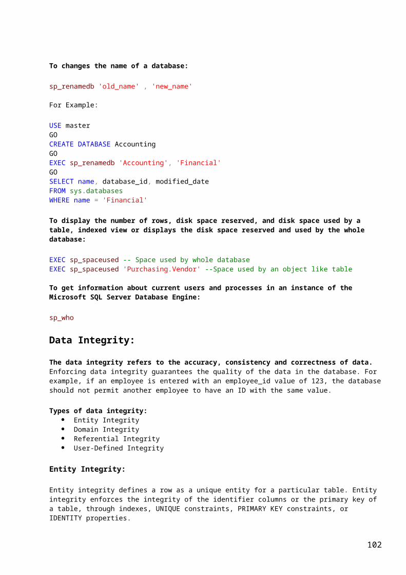
Or

select * from HumanResources.JobCandidatewhere Freetext(Resume,'%Considerable%')

Try using like poerator

select * from HumanResources.JobCandidatewhere Resume like '%Considerable%'

Msg 8116, Level 16, State 1, Line 1Argument data type xml is invalid for argument 1 of like function.

To create an Full-Index in management studio, follow the steps:

Create a Full-Text Catalog Create a Full-Text Index Populate the Index

Create a Full-Text Catalog

Expand the desired database Expand the storage Right click on the full-text catalog Provide catalog name and other information required Click OK

Your fulltext catalog is created.Create a Full-Text Index

Right click on the table name Click on the ‘Define FULL-Text Index’ in context menu Select unique index for Key index (if not available, first create it before

starting Full-Text Index Creation) Check on character-based column on which the full-text index is to be

created Select ‘tract change automatically’ Select full-text catalog name in which you want to group this index OR

check on create new catalog and provide required information finish

Populate the Index

Right click on table name on which the full-text index is created. Click on full-test index Click on “Start Full Population”

Suppose you did all these things on HumanResources.Employee table.

Now try the following queries:

SELECT BusinessEntityID, JobTitleFROM HumanResources.EmployeeWHERE FREETEXT(*, 'Marketing Assistant');

SELECT BusinessEntityID,JobTitleFROM HumanResources.EmployeeWHERE CONTAINS(JobTitle, 'Marketing OR Assistant');

SELECT BusinessEntityID,JobTitleFROM HumanResources.EmployeeWHERE CONTAINS(JobTitle, 'Marketing AND Assistant');

102

Example to create othe indexes:

Creating a simple nonclustered index

IF EXISTS (SELECT name FROM sys.indexes WHERE name = 'IX_ProductVendor_VendorID') DROP INDEX IX_ProductVendor_VendorID ON Purchasing.ProductVendor;

CREATE INDEX IX_ProductVendor_VendorID ON Purchasing.ProductVendor (VendorID);

Creating a simple nonclustered composite index:

IF EXISTS (SELECT name FROM sys.indexes WHERE name = 'IX_SalesPerson_SalesQuota_SalesYTD') DROP INDEX IX_SalesPerson_SalesQuota_SalesYTD ON Sales.SalesPerson ;

CREATE NONCLUSTERED INDEX IX_SalesPerson_SalesQuota_SalesYTDON Sales.SalesPerson (SalesQuota, SalesYTD);

Creating a unique nonclustered index

IF EXISTS (SELECT name from sys.indexes WHERE name = 'AK_UnitMeasure_Name') DROP INDEX AK_UnitMeasure_Name ON Production.UnitMeasure;

CREATE UNIQUE INDEX AK_UnitMeasure_Name ON Production.UnitMeasure(Name);

Using DROP_EXISTING to drop and re-create an index

The following example drops and re-creates an existing index on the ProductID column of the Production.WorkOrder table by using the DROP_EXISTING option. The options FILLFACTOR and PAD_INDEX are also set.

CREATE NONCLUSTERED INDEX IX_WorkOrder_ProductID ON Production.WorkOrder(ProductID) WITH (FILLFACTOR = 80, PAD_INDEX = ON, DROP_EXISTING = ON);

Creating an index on a view

--Set the options to support indexed views.SET NUMERIC_ROUNDABORT OFF;SET ANSI_PADDING, ANSI_WARNINGS, CONCAT_NULL_YIELDS_NULL, ARITHABORT, QUOTED_IDENTIFIER, ANSI_NULLS ON;GO--Create view with schemabinding.IF OBJECT_ID ('Sales.vOrders', 'view') IS NOT NULLDROP VIEW Sales.vOrders ;GOCREATE VIEW Sales.vOrdersWITH SCHEMABINDINGAS SELECT SUM(UnitPrice*OrderQty*(1.00-UnitPriceDiscount)) AS Revenue, OrderDate, ProductID, COUNT_BIG(*) AS COUNT FROM Sales.SalesOrderDetail AS od, Sales.SalesOrderHeader AS o WHERE od.SalesOrderID = o.SalesOrderID GROUP BY OrderDate, ProductID;GO--Create an index on the view.CREATE UNIQUE CLUSTERED INDEX IDX_V1 ON Sales.vOrders (OrderDate, ProductID);

103

Creating an index with included (nonkey) columns

The following example creates a nonclustered index with one key column (PostalCode) and four nonkey columns (AddressLine1, AddressLine2, City, StateProvinceID).

IF EXISTS (SELECT name FROM sys.indexes WHERE name = 'IX_Address_PostalCode') DROP INDEX IX_Address_PostalCode ON Person.Address;

CREATE NONCLUSTERED INDEX IX_Address_PostalCode ON Person.Address (PostalCode) INCLUDE (AddressLine1, AddressLine2, City, StateProvinceID);

Showing the complete table definition:The following example shows the complete table definitions with all constraint definitions for table PurchaseOrderDetail created in the AdventureWorks database.

CREATE TABLE [dbo].[PurchaseOrderDetail]( [PurchaseOrderID] [int] NOT NULL REFERENCES Purchasing.PurchaseOrderHeader(PurchaseOrderID), [LineNumber] [smallint] NOT NULL, [ProductID] [int] NULL REFERENCES Production.Product(ProductID), [UnitPrice] [money] NULL, [OrderQty] [smallint] NULL, [ReceivedQty] [float] NULL, [RejectedQty] [float] NULL, [DueDate] [datetime] NULL, [rowguid] [uniqueidentifier] ROWGUIDCOL NOT NULL CONSTRAINT [DF_PurchaseOrderDetail_rowguid] DEFAULT (newid()), [ModifiedDate] [datetime] NOT NULL CONSTRAINT [DF_PurchaseOrderDetail_ModifiedDate] DEFAULT (getdate()), [LineTotal] AS (([UnitPrice]*[OrderQty])), [StockedQty] AS (([ReceivedQty]-[RejectedQty])),CONSTRAINT [PK_PurchaseOrderDetail_PurchaseOrderID_LineNumber] PRIMARY KEY CLUSTERED ([PurchaseOrderID], [LineNumber]) WITH (IGNORE_DUP_KEY = OFF)) ON [PRIMARY]

View:A view is a virtual table whose contents are defined by a query. Like a real table, a view consists of a set of named columns and rows of data. Unless indexed, a view does not exist as a stored set of data values in a database. The rows and columns of data come from tables referenced in the query defining the view and are produced dynamically when the view is referenced.

A view acts as a filter on the underlying tables referenced in the view. The query that defines the view can be from one or more tables or from other views in the current or other databases.

This illustration shows a view based on two tables.

104

Why do we need a view?

Views can be used as security mechanisms by letting users’ access data through the view, without granting the users permissions to directly access the underlying base tables of the view.

Views can simplify how users work with data. You can define frequently used joins, projections, UNION queries, and SELECT queries as views so that users do not have to specify all the conditions and qualifications every time an additional operation is performed on that data. For example, a complex query that is used for reporting purposes and performs subqueries, outer joins, and aggregation to retrieve data from a group of tables can be created as a view. The view simplifies access to the data because the underlying query does not have to be written or submitted every time the report is generated; the view is queried instead.

Example of view:

CREATE VIEW vBikes ASSELECT DISTINCT p.[Name] FROM Production.Product p JOIN Production.ProductInventory i ON p.ProductID = i.ProductID JOIN Production.ProductSubCategory ps ON p.ProductSubcategoryID = ps.ProductSubCategoryID JOIN Production.ProductCategory pc ON (ps.ProductCategoryID = pc.ProductCategoryID AND pc.Name = 'Bikes') AND i.Quantity > 0

Types of views

Standard Views

Standard views are simple view. See the above for example.

Indexed Views

An indexed view is a view that has been materialized. This means it has been computed and stored. You index a view by creating a unique clustered index on it. Indexed views dramatically improve the performance of some types of queries. Indexed views work best for queries that aggregate many rows. They are not well-suited for underlying data sets that are frequently updated.

105

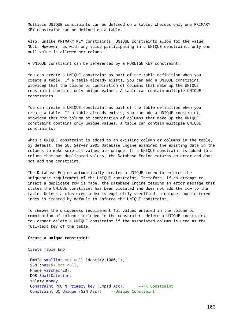
A view must meet the following requirements before you can create a clustered index on it:

The ANSI_NULLS and QUOTED_IDENTIFIER options must have been set to ON when the CREATE VIEW statement was executed. The OBJECTPROPERTY function reports this for views through the ExecIsAnsiNullsOn or ExecIsQuotedIdentOn properties.

The ANSI_NULLS option must have been set to ON for the execution of all CREATE TABLE statements that create tables referenced by the view.

The view must not reference any other views, only base tables.

All base tables referenced by the view must be in the same database as the view and have the same owner as the view.

The view must be created with the SCHEMABINDING option. Schema binding binds the view to the schema of the underlying base tables.

User-defined functions referenced in the view must have been created with the SCHEMABINDING option.

Tables and user-defined functions must be referenced by two-part names in the view. One-part, three-part, and four-part names are not allowed. (schema_Name.Table_Name is correct)

See Page 103 for Example of indexed view

Partitioned Views:

A partitioned view joins horizontally partitioned data from a set of member tables across one or more servers. This makes the data appear as if from one table. A view that joins member tables on the same instance of SQL Server is a local partitioned view.

Note:Imposible to practice in a single server.

SQL and T-SQL:

SQL is an ANSI standard query language which is used by all databases. For example:

Select * from Table_Name

T-SQL (Transact-SQL):

T-SQL (Transact-SQL) is a set of programming extensions from Sybase and Microsoft that add several features to the Structured Query Language (SQL) including transaction control, exception and error handling, row processing, and declared variables. Microsoft's SQL Server and Sybase's SQL server support T-SQL statements.

1 Flow control 2 Local variables 3 Changes to DELETE and UPDATE statements 4 BULK INSERT

Transact-SQL includes:

BEGIN and ENDBREAK and CONTINUE

106

GOTOIF and ELSERETURNWAITFORWHILE

The above mentioned keywords are not used in simple SQL statements.

One T-SQL Example:

IF DATEPART(dw, GETDATE()-3) = 7 OR DATEPART(dw, GETDATE()) = 1BEGIN PRINT 'It is the weekend.' PRINT 'Get some rest!'ENDELSEBEGIN PRINT 'It is a weekday.' PRINT 'Get to work!'END

Output:

It is the weekend.Get some rest!

One more example for T-SQL:

DECLARE @Counter INTSET @Counter = 10WHILE @Counter > 0BEGIN PRINT 'The count is ' + CONVERT(VARCHAR(10), @Counter) SET @Counter = @Counter - 1END

Output:

The count is 10The count is 9The count is 8The count is 7The count is 6The count is 5The count is 4The count is 3The count is 2The count is 1

In Transact-SQL, both the DELETE and UPDATE statements allow a FROM clause to be added, which allows joins to be included.

This example deletes all users who have been flagged with the 'Idle' flag.

It is not allowed in Oracle.

DELETE users FROM users AS u JOIN user_flags AS f ON u.id=f.id WHERE f.name = 'Idle'

Common Table Expression(CTE):CTE specifies a temporary named result set, known as a common table expression (CTE). This is derived from a simple query and defined within the execution scope of a SELECT, INSERT, UPDATE, or DELETE statement. This clause can also be used in

107

a CREATE VIEW statement as part of its defining SELECT statement. A common table expression can include references to itself. This is referred to as a recursive common table expression.

Syntax: WITH CTE_Name(Col1, Col2, Col3, Col4,. . . .) AS ( CTE_query_definition)

Select Col1, Col2, Col3, Col4 from CTE_Name

Example:

WITH DirReps(ManagerID, DirectReports) AS ( SELECT ManagerID, COUNT(*) FROM HumanResources.Employee AS e WHERE ManagerID IS NOT NULL GROUP BY ManagerID)SELECT ManagerID, DirectReports FROM DirReps ORDER BY ManagerID

CTE_query_definition:

It specifies a SELECT statement whose result set populates the common table expression. The SELECT statement for CTE_query_definition must meet the same requirements as for creating a view, except a CTE cannot define another CTE

If more than one CTE_query_definition is defined, the query definitions must be joined by one of these set operators: UNION ALL, UNION, EXCEPT, or INTERSECT

Guidelines for Creating and Using CTEsThe following guidelines apply to nonrecursive CTEs

A CTE must be followed by a SELECT, INSERT, UPDATE, or DELETE statement that references some or all the CTE columns. A CTE can also be specified in a CREATE VIEW statement as part of the defining SELECT statement of the view.

Multiple CTE query definitions can be defined in a nonrecursive CTE. The definitions must be combined by one of these set operators: UNION ALL, UNION, INTERSECT, or EXCEPT.

A CTE can reference itself and previously defined CTEs in the same WITH clause. Forward referencing is not allowed.

Specifying more than one WITH clause in a CTE is not allowed.

For example, if a CTE_query_definition contains a subquery, that subquery cannot contain a nested WITH clause that defines another CTE.

The following clauses cannot be used in the CTE_query_definition:

COMPUTE or COMPUTE BYORDER BY (except when a TOP clause is specified)INTO OPTION clause with query hintsFOR XMLFOR BROWSE

108

When a CTE is used in a statement that is part of a batch, the statement before it must be followed by a semicolon.

Note: Tables on remote servers can be referenced in the CTE.

Examples

A.Creating a simple common table expressionThe following example shows the number of employees reporting directly to each manager at Adventure Works Cycles.

WITH DirReps(ManagerID, DirectReports) AS ( SELECT ManagerID, COUNT(*) FROM HumanResources.Employee AS e WHERE ManagerID IS NOT NULL GROUP BY ManagerID)SELECT ManagerID, DirectReports FROM DirReps ORDER BY ManagerID;

B. Using a common table expression to limit counts and report averagesThe following example shows the average number of employees reporting to managers.

WITH DirReps (Manager, DirectReports) AS ( SELECT ManagerID, COUNT(*) AS DirectReports FROM HumanResources.Employee GROUP BY ManagerID)

SELECT AVG(DirectReports) AS [Average Number of Direct Reports]FROM DirReps WHERE DirectReports>= 2 ;

C. Referencing a common table expression more than one time:

The following example shows the total number of sales orders and the most recent sales order date in the SalesOrderHeader table for each salesperson. In the running statement, the CTE is referenced two times: one time to return the selected columns for the salesperson, and again to retrieve similar details for the salesperson's manager. The data for both the salesperson and the manager are returned in a single row.

WITH Sales_CTE (SalesPersonID, NumberOfOrders, MaxDate)AS( SELECT SalesPersonID, COUNT(*), MAX(OrderDate) FROM Sales.SalesOrderHeader GROUP BY SalesPersonID)SELECT E.EmployeeID, OS.NumberOfOrders, OS.MaxDate, E.ManagerID, OM.NumberOfOrders, OM.MaxDateFROM HumanResources.Employee AS E JOIN Sales_CTE AS OS ON E.EmployeeID = OS.SalesPersonID LEFT OUTER JOIN Sales_CTE AS OM ON E.ManagerID = OM.SalesPersonIDORDER BY E.EmployeeID;

Do it At leasure Time*****************************

109

Guidelines for Defining and Using Recursive CTEs

The recursive CTE definition must contain at least two CTE query definitions:

An anchor member Recursive member

Multiple anchor members and recursive members can be defined; however, all anchor member query definitions must be put before the first recursive member definition.

All CTE query definitions are anchor members unless they reference the CTE itself.

Anchor members must be combined by one of these set operators: UNION ALL, UNION, INTERSECT, or EXCEPT. UNION ALL is the only set operator allowed between the last anchor member and first recursive member, and when combining multiple recursive members.

The number of columns in the anchor and recursive members must be the same.

The data type of a column in the recursive member must be the same as the data type of the corresponding column in the anchor member.

The FROM clause of a recursive member must refer only one time to the CTE expression_name.

The following items are not allowed in the CTE_query_definition of a recursive member:

SELECT DISTINCT GROUP BY HAVING Scalar aggregation TOP LEFT, RIGHT, OUTER JOIN (INNER JOIN is allowed) Subqueries

The following guidelines apply to using a recursive CTE:

An incorrectly composed recursive CTE may cause an infinite loop. For example, if the recursive member query definition returns the same values for both the parent and child columns, an infinite loop is created.

To prevent an infinite loop, you can limit the number of recursion levels allowed for a particular statement by using the MAXRECURSION hint and a value between 0 and 32,767 in the OPTION clause of the INSERT, UPDATE, DELETE, or SELECT statement. This lets you control the execution of the statement until you resolve the code problem that is creating the loop. The server-wide default is 100. When 0 is specified, no limit is applied. Only one MAXRECURSION value can be specified per statement. For more information, see Query Hint (Transact-SQL).

A view that contains a recursive common table expression cannot be used to update data.

Cursors may be defined on queries using CTEs. Only fast forward-only and static (snapshot) cursors are allowed for recursive CTEs.

If another cursor type is specified in a recursive CTE, the cursor type is converted to static.

D. Using a recursive common table expression to display multiple levels of recursionThe following example shows the hierarchical list of managers and the employees who report to them.

110

WITH DirectReports(ManagerID, EmployeeID, EmployeeLevel) AS ( SELECT ManagerID, EmployeeID, 0 AS EmployeeLevel FROM HumanResources.Employee WHERE ManagerID IS NULL UNION ALL SELECT e.ManagerID, e.EmployeeID, EmployeeLevel + 1 FROM HumanResources.Employee e INNER JOIN DirectReports d ON e.ManagerID = d.EmployeeID )SELECT ManagerID, EmployeeID, EmployeeLevel FROM DirectReports ;

E. Using a recursive common table expression to display two levels of recursionThe following example shows managers and the employees reporting to them. The number of levels returned is limited to two.

WITH DirectReports(ManagerID, EmployeeID, EmployeeLevel) AS ( SELECT ManagerID, EmployeeID, 0 AS EmployeeLevel FROM HumanResources.Employee WHERE ManagerID IS NULL UNION ALL SELECT e.ManagerID, e.EmployeeID, EmployeeLevel + 1 FROM HumanResources.Employee e INNER JOIN DirectReports d ON e.ManagerID = d.EmployeeID )SELECT ManagerID, EmployeeID, EmployeeLevel FROM DirectReports WHERE EmployeeLevel <= 2 ;

F. Using a recursive common table expression to display a hierarchical listThe following example builds on Example C by adding the names of the manager and employees, and their respective titles. The hierarchy of managers and employees is additionally emphasized by indenting each level.

WITH DirectReports(Name, Title, EmployeeID, EmployeeLevel, Sort)AS (SELECT CONVERT(varchar(255), c.FirstName + ' ' + c.LastName), e.Title, e.EmployeeID, 1, CONVERT(varchar(255), c.FirstName + ' ' + c.LastName) FROM HumanResources.Employee AS e JOIN Person.Contact AS c ON e.ContactID = c.ContactID WHERE e.ManagerID IS NULL UNION ALL SELECT CONVERT(varchar(255), REPLICATE ('| ' , EmployeeLevel) + c.FirstName + ' ' + c.LastName), e.Title, e.EmployeeID, EmployeeLevel + 1, CONVERT (varchar(255), RTRIM(Sort) + '| ' + FirstName + ' ' + LastName) FROM HumanResources.Employee as e JOIN Person.Contact AS c ON e.ContactID = c.ContactID JOIN DirectReports AS d ON e.ManagerID = d.EmployeeID )SELECT EmployeeID, Name, Title, EmployeeLevelFROM DirectReports ORDER BY Sort;

111

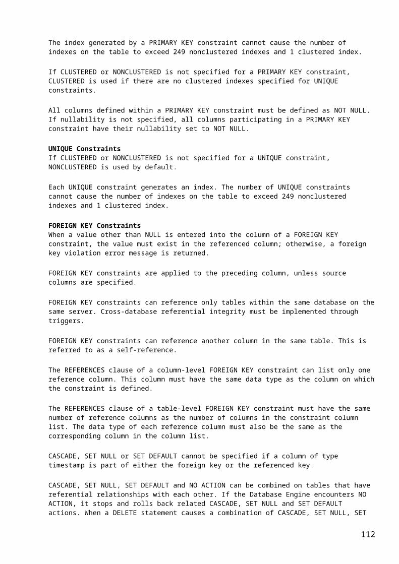
G. Using MAXRECURSION to cancel a statementMAXRECURSION can be used to prevent a poorly formed recursive CTE from entering into an infinite loop. The following example intentionally creates an infinite loop and uses the MAXRECURSION hint to limit the number of recursion levels to two.

--Creates an infinite loopWITH cte (EmployeeID, ManagerID, Title) as( SELECT EmployeeID, ManagerID, Title FROM HumanResources.Employee WHERE ManagerID IS NOT NULL UNION ALL SELECT cte.EmployeeID, cte.ManagerID, cte.Title FROM cte JOIN HumanResources.Employee AS e ON cte.ManagerID = e.EmployeeID)--Uses MAXRECURSION to limit the recursive levels to 2SELECT EmployeeID, ManagerID, TitleFROM cteOPTION (MAXRECURSION 2);

After the coding error is corrected, MAXRECURSION is no longer required. The following example shows the corrected code.

WITH cte (EmployeeID, ManagerID, Title)AS( SELECT EmployeeID, ManagerID, Title FROM HumanResources.Employee WHERE ManagerID IS NOT NULL UNION ALL SELECT e.EmployeeID, e.ManagerID, e.Title FROM HumanResources.Employee AS e JOIN cte ON e.ManagerID = cte.EmployeeID)SELECT EmployeeID, ManagerID, TitleFROM cte;H. Using a common table expression to selectively step through a recursive relationship in a SELECT statementThe following example shows the hierarchy of product assemblies and components that are required to build the bicycle for ProductAssemblyID = 800.

WITH Parts(AssemblyID, ComponentID, PerAssemblyQty, EndDate, ComponentLevel) AS( SELECT b.ProductAssemblyID, b.ComponentID, b.PerAssemblyQty, b.EndDate, 0 AS ComponentLevel FROM Production.BillOfMaterials AS b WHERE b.ProductAssemblyID = 800 AND b.EndDate IS NULL UNION ALL SELECT bom.ProductAssemblyID, bom.ComponentID, p.PerAssemblyQty, bom.EndDate, ComponentLevel + 1 FROM Production.BillOfMaterials AS bom INNER JOIN Parts AS p ON bom.ProductAssemblyID = p.ComponentID AND bom.EndDate IS NULL)SELECT AssemblyID, ComponentID, Name, PerAssemblyQty, EndDate, ComponentLevel FROM Parts AS p INNER JOIN Production.Product AS pr ON p.ComponentID = pr.ProductID

112

ORDER BY ComponentLevel, AssemblyID, ComponentID;

I. Using a recursive CTE in an UPDATE statementThe following example updates the VacationHours value by 25 percent for all employees who report directly or indirectly to ManagerID 12. The common table expression returns a hierarchical list of employees who report directly to ManagerID 12 and employees who report to those employees, and so on. Only the rows returned by the common table expression are modified.

WITH DirectReports(EmployeeID, NewVacationHours, EmployeeLevel)AS(SELECT e.EmployeeID, e.VacationHours, 1 FROM HumanResources.Employee AS e WHERE e.ManagerID = 12 UNION ALL SELECT e.EmployeeID, e.VacationHours, EmployeeLevel + 1 FROM HumanResources.Employee as e JOIN DirectReports AS d ON e.ManagerID = d.EmployeeID)UPDATE HumanResources.EmployeeSET VacationHours = VacationHours * 1.25FROM HumanResources.Employee AS eJOIN DirectReports AS d ON e.EmployeeID = d.EmployeeID;

J. Using multiple anchor and recursive membersThe following example uses multiple anchor and recursive members to return all the ancestors of a specified person. A table is created and values inserted to establish the family genealogy returned by the recursive CTE.

IF OBJECT_ID('Person','U') IS NOT NULL DROP TABLE Person;CREATE TABLE Person(ID int, Name varchar(30), Mother int, Father int);INSERT Person VALUES(1, 'Sue', NULL, NULL);INSERT Person VALUES(2, 'Ed', NULL, NULL);INSERT Person VALUES(3, 'Emma', 1, 2);INSERT Person VALUES(4, 'Jack', 1, 2);INSERT Person VALUES(5, 'Jane', NULL, NULL);INSERT Person VALUES(6, 'Bonnie', 5, 4);INSERT Person VALUES(7, 'Bill', 5, 4);-- Create the recursive CTE to find all of Bonnie's ancestors.WITH Generation (ID) AS(-- First anchor member returns Bonnie's mother. SELECT Mother FROM Person WHERE Name = 'Bonnie'UNION-- Second anchor member returns Bonnie's father. SELECT Father FROM Person WHERE Name = 'Bonnie'UNION ALL-- First recursive member returns male ancestors of the previous generation. SELECT Person.Father FROM Generation, Person WHERE Generation.ID=Person.IDUNION ALL-- Second recursive member returns female ancestors of the previous generation. SELECT Person.Mother FROM Generation, Person WHERE Generation.ID=Person.ID)SELECT Person.ID, Person.Name, Person.Mother, Person.FatherFROM Generation, PersonWHERE Generation.ID = Person.ID;

113

Programming in SQL Server:

Batch:

A batch is one or multiple T-SQL statements that is executed by sql server as a single unit. SQL Server compiles the batch into a single executable unit called an execution plan. Batches are separated by a GO statement, which marks the end of one batch and beginning of another.

In simple words:

Any sql statement or a group of statements terminated by ‘GO’ is a batch.

Batches are of two types: Anonymous batches and Named batches.Anonymous batches:

A batch without any name is called as anonymous batch.

Syntax:

[Begin] ----- SQL Statements----- ----- [End]GO

Example

begindeclare @aa intset @aa=5select @aa*10endgo

Named batches:Again named batches are devided into 3 types:

Stored procedures. Functions. Triggers.

114

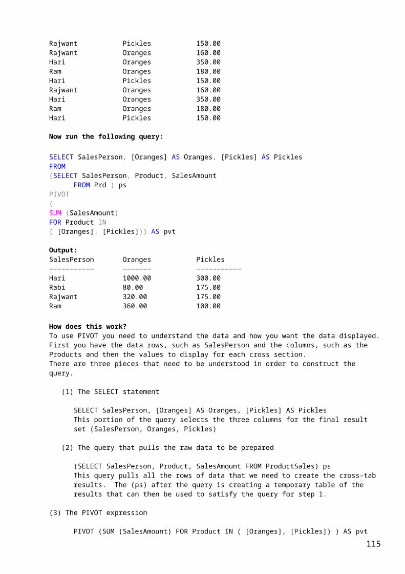
Rules of batches:

If there is a syntax error anywhere in the batch, none of the statements is executed. For example, here is a batch with a typing error in the last statement, and the results:

select count(*) from titles select count(*) from authors slect count(*) from publishers go

Msg 156, Level 15, State 1: Line 3:Incorrect syntax near the keyword 'count'.

Before referencing objects in a database, issue a use statement for that database. For example:

use master go

select count(*) from sysdatabases go

You cannot drop and recreate the same object in a single batch:

Example:

drop procedure ppppcreate procedure pppp asselect * from Salgo

Msg 111, Level 15, State 1, Procedure pppp, Line 3'CREATE/ALTER PROCEDURE' must be the first statement in a query batch.

You cannot combine the following database commands with other statements in a batch:

create procedure create rule create default create trigger

For example:Create a table as follows

create table aa(fname varchar(20),age int)go

Create a procedure and drop the created table aa in the same procedure as :

create procedure pppp asselect * from Saldrop table aago

Here you will not get error because sybtax is correct but it will create the procedure and will not delete the table.

115

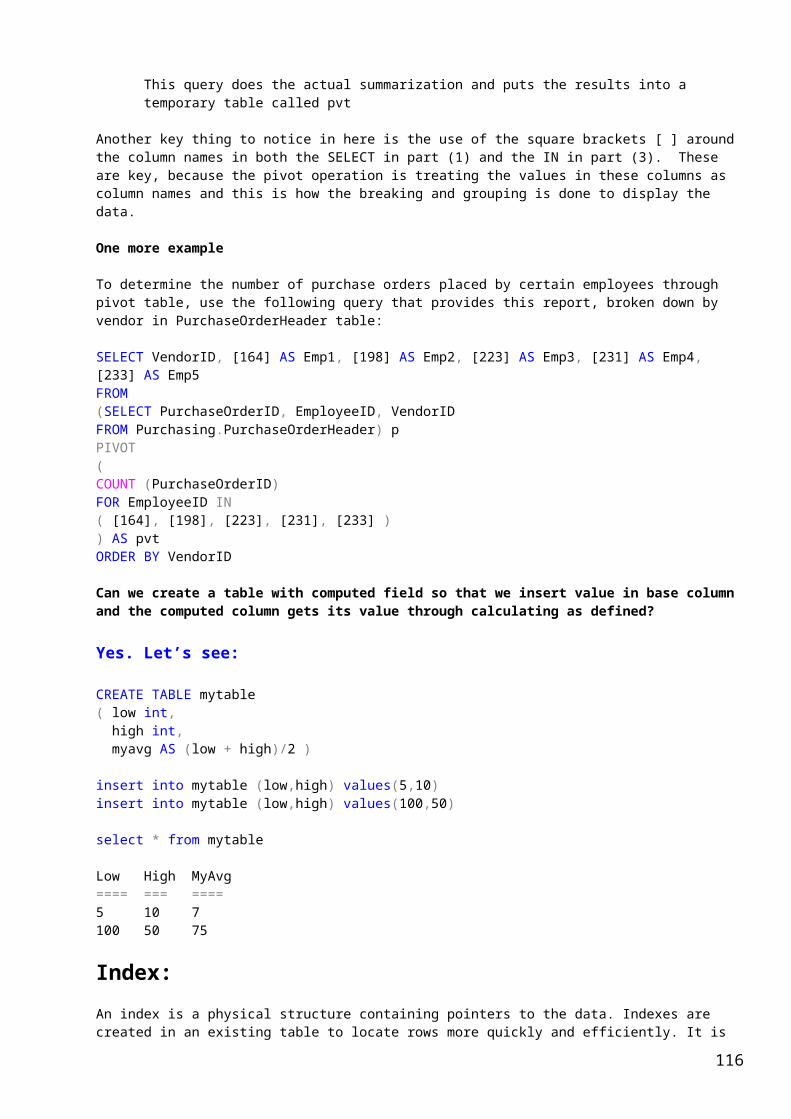
You can combine the following database commands with other Transact-SQL statements in a batch:

create database (except that you cannot create a database and create or access objects in the new database in a single batch)

create table create index create view

for example: create a table and insert data in new table from existing table as:

create table NewSalary(impid varchar(20),SalDate datetime,Sal int)insert into NewSalaryselect * from salgo

It is allowed.

You cannot reference a new column in other sql statements in the same batch that is added altering the table:

Example:this is not allowed.

Alter table tab1add test_id intselect test_id from tab1go

You can create a table and reference it in the same batch. This batch creates a table, inserts a row into it, and then selects everything from it:

create table test (column1 char(10), column2 int) insert test values ("hello", 598) select * from test go

You can combine a drop statement with other statements as long as you do not reference or re-create the dropped object in the same batch. This example combines a drop statement with a select statement:

drop table test select count(*) from titles go

Batches that violate a batch rule also generate error messages. Here are some examples of illegal batches:

create table test (column1 char(10), column2 int) insert test values ("hello", 598) select * from test create procedure testproc as select column1 from test go

Msg 111, Level 15, State 7: Line 6: CREATE PROCEDURE must be the first command in a

116

query batch.

Using control-of-flow language

Use control-of-flow language with interactive statements, in batches, and in stored procedures.

Control-of-flow and related keywords with their functions: if Defines conditional execution. ...else Defines alternate execution when the if condition is false. case Defines conditional expressions using when...then statements instead of if...else. begin Beginning of a statement block. ...end End of a statement block. while Repeat performance of statements while condition is true. break Exit from the end of the next outermost while loop. ...continue Restart while loop. goto label Go to label:, a position in a statement block. return Exit unconditionally. waitfor Set delay for command execution. print Print a user-defined message or local variable on user's screen. Examples of control-of-flow language:

if...elseThe keyword if, with or without its companion else, introduces a condition that determines whether the next statement is executed. The Transact-SQL statement executes if the condition is satisfied, that is, if it returns TRUE.

The else keyword introduces an alternate Transact-SQL statement that executes when the if condition returns FALSE.

The syntax for if and else is:

if boolean_expression statement [else [if boolean_expression]

117

statement ]

A Boolean expression returns TRUE or FALSE. It can include a column name, a constant, any combination of column names and constants connected by arithmetic operators, or a subquery, as long as the subquery returns a single value. If the Boolean expression contains a select statement, the select statement must be enclosed in parentheses, and it must return a single value.

Here is an example of using if alone:

if exists (select * from Person.Contact where FirstName = 'Gustavo') select 'First Name of Contact person is ' + cast(FirstName as varchar (20)) as Contact_Person from Person.Contact

where FirstName = 'Gustavo'

Output:Contact_Person===========================================First Name of Contact person is Gustavo

Here is an example, using both if and else”

if exists (select * from Person.Contact where FirstName = 'Gustavo')

beginPrint 'First Name of Contact person is ' select cast(FirstName as varchar (20)) as Contact_Person from Person.Contact

where FirstName = 'Gustavo'end

elseprint 'Name not available'

Output:

Contact_Person==================GustavoGustavo

Another example that tests for the presence of user-created objects that have ID numbers greater than 50. If user objects exist, the else clause selects their names, types, and ID numbers.

if (select max(id) from sysobjects) < 50 print 'There are no user-created objects in this database.'else select name, type, id from sysobjects where id > 50 and type = 'U'go name type id ------------ ---- --------- ProductProductPhoto U 18099105StoreContact U 30623152Address U 53575229ProductReview U 66099276TransactionHistory U 78623323AddressType U 101575400ProductSubcategory U 130099504AWBuildVersion U 149575571

case expression118

Case expression simplifies many conditional Transact-SQL constructs. Instead of using a series of if statements, case expression allows you to use a series of conditions that return the appropriate values when the conditions are met. case expression is ANSI SQL92 compliant.

With case expression, you can:

Simplify queries and write more efficient code Convert data between the formats used in the database (such as int) and the

format used in an application (such as char) Return the first non-null value in a list of columns Compare two values and return the first value if the values do not match,

or a NULL value if the values do match Write queries that avoid division by 0

Case expression includes the keywords case, when, then, coalesce, and nullif.

Case and division by zeroFirst create the following table in your test Database and insert the following data.

create table Sale(P_Id char(5),P_Name varchar (20),Unit_Price int,Qty int,TotalPrice AS (Unit_Price * Qty),Discount int)

select * from Sale

P_Id P_Name Unit_Price Qty TotalPrice Discount===== ====== ========== === ========== ========1001 AAA 10 2 20 51002 BBB 15 5 75 601003 CCC 2 1 2 01004 DDD 5 1 5 01005 EEE 2 2 4 01006 FFF 1 50 50 1Note: No need to feed data for TotalPrice field because it is table calculated field.

Way to insert value:insert into Sale (P_id,P_Name,Unit_Price,Qty,Discount) values('1006','FFF',1,50,1)

Case and division by zeroCase expression allows you to write queries that avoid division by zero (called exception avoidance). For example, if you attempt to divide the total_sales value column for each sale by the discount column, the query results error msg “Divide by zero occurred”.

Run the following query:select TotalPrice/Discount from Sale

Output:Msg 8134, Level 16, State 1, Line 1Divide by zero error encountered.

So you can use a case expression to avoid this by not allowing the zero to figure in the equation. In this example, when the query comes across the zero, it returns a predefined value, rather than performing the division:

select TotalPrice, Discount, "Discount on per TotalPrice " =

119

case when Discount != 0 then convert(char, TotalPrice / Discount) else 'No Discount' endfrom Sale

TotalPrice Discount Discount on per TotalPrice-------- -------- --------------------------20 5 4 75 60 1 2 0 No Discount5 0 No Discount4 0 No Discount50 1 50

Note:

Unlike other languages, TSQL does not have an ELSE IF key word. The work around is to nest IF...ELSE statements inside other IF...ELSE statements. There are no limits to the number of times an IF...ELSE statement can be nested. There is no END IF statement in SQL Server.

BEGIN...ENDThe BEGIN and END keywords are used to group multiple lines into one Statement Block. An example of when Statement Blocks are required is in the result of an IF ELSE statement. In this example, two PRINT lines are wanted on True result.

if exists (select * from Person.Contact where FirstName = 'Gustavo')

beginPrint 'First Name of Contact person is ' --Statement 1select cast(FirstName as varchar (20)) as Contact_Person from Person.Contact

where FirstName = 'Gustavo' --Statement 2end

elseprint 'Name not available'

Note:

As per the above statement, if first name is not available in the table, if statement is not executed, else statement is executed and the message is printed as 'Name not available'.

GOTO label

GOTO works like a loop. It simply defines a label, and lets the code jump to that label from some other point. Cursors usually make use of a GOTO statement. However, a GOTO can also be used alone. It defines a GOTO Label, do_it_again, by ending it with a colon. When the second IF is executed, GOTO sends control back to the Label until the defined condition is not fulfilled.

For Example:How can I print “Hello Friends” ten times without Loop?

DECLARE @Count intSET @Count = 0

do_it_again: --label for Goto IF @Count < 10

BEGIN PRINT 'Hello Friends' SET @Count = @Count + 1END

120

IF @Count < 10

GOTO do_it_again

This code prints ‘Hello Friends’ 10 times.

Return

The RETURN key word ends the statements execution unconditionally. Any lines following a RETURN are not executed. If a RETURN is placed inside our Label code, only one "Hello Friends" will be printed.

Example:

DECLARE @Count intSET @Count = 0

do_it_again: --label for Goto IF @Count < 10

BEGIN PRINT 'Hello Friends' RETURN --Will not be executed from here to downward SET @Count = @Count + 1END

IF @Count < 10

GOTO do_it_againgo

Waitfor

WAITFOR allows statement execution to be paused for a delayed time amount, or until a specific time of day.

Syntax: Waitfor {Delay|Time SQL Statements}

Delay: It is the specified period of time that must pass before execution of T-SQL Statements.

TIME: Is the specified time when the T-SQL Statements (Batch or procedures) start to run.

Using Waitfor Delay:

beginWaitfor Delay '00:02:00'execute sp_helpdb

end

This will give output after 2 minutes (even if its internal execution plan is already finished, it stores the output in buffer and displays after elapsing the specified period)

Using Waitfor Time:

beginWaitfor Time '13:38:00 PM'execute sp_helpdb

end

This will start to execute at '13:38:00 PM'

121

Note: Waitfor statement is used for sys-admin activity like backup of data at fix time each day.

WHILE

While sets a condition for the repeated execution of SQL Statements or statement blok. The statements are executed repeatedly as long as the specified condition is true. BEGIN and END are also used in the same IF statement way.

DECLARE @Count intSET @Count = 0

WHILE @Count < 100 BEGIN

PRINT 'Hello Friends'SET @Count = @Count + 1

END

BREAK...CONTINUEBREAK and CONTINUE are used to exit, or continue executing WHILE or IF statements. The above statements have been modified to show an example of their use. The statement will only return ten rows now.

DECLARE @Count intSET @Count = 0

WHILE @Count < 100 BEGIN

PRINT 'Hello Friends'SET @Count = @Count + 1IF @Count > 10 BREAKELSE

CONTINUE END

Cursor:Cursor is a database object used by applications to manipulate data in a set on a row-by-row basis, instead of the typical SQL commands that operate on all the rows in the set at one time. The cursor comes with set of rows together with a pointer that identifies a current row. We can access a single row or ‘N’ number of rows with the help of cursor.

Before using cursor, you first must declare the cursor. Once a cursor has been declared, you can open it and fetch from it. You can fetch row by row and make multiple operations on the currently active row in the cursor. When you have finished working with a cursor, you should close cursor and deallocate it to release SQL Server resources.

Syntax to write cursor:

DECLARE cursor_name CURSOR[LOCAL | GLOBAL][FORWARD_ONLY | SCROLL][STATIC | KEYSET | DYNAMIC | FAST_FORWARD][READ_ONLY | SCROLL_LOCKS | OPTIMISTIC][TYPE_WARNING]FOR select_statement[FOR UPDATE [OF column_name [,...n]]]

Explanation of Keywords:

122

cursor_name - The name of the server side cursor, must contain from 1 to 128 characters.

Scope of cursor:

Microsoft SQL Server 2005 supports the GLOBAL and LOCAL keywords on the DECLARE CURSOR statement to define the scope of the cursor name

LOCAL - Specifies that cursor can be available only in the batch, stored procedure, or trigger in which the cursor was created. The LOCAL cursor will be implicitly deallocated when the batch, stored procedure, or trigger terminates.

GLOBAL - Specifies that cursor is global to the connection. The GLOBAL cursor will be implicitly deallocated at disconnect.

Types of cursor:

Cursor’s type determines the cursor’s behaviour.

FORWARD_ONLY - Specifies that cursor can only fetch data sequentially from the first to the last row. FETCH NEXT is the only fetch option supported.

STATIC - Specifies that cursor will use a temporary copy of the data instead of base tables. This cursor does not allow modifications and modifications made to base tables are not reflected in the data returned by fetches made to this cursor.

KEYSET - KEYSET Cursor uses the set of keys that are primary that uniquely identify the cursor's rows. SQL Server uses a table in tempdb to store keyset. The KEYSET cursor helps to updates non key values from being made through this cursor, but when inserts made by other users are not visible. Updates nonkey values made by other users are visible as the owner scrolls around the cursor, but updates key values made by other users are not visible

DYNAMIC - Specifies that cursor reflects all data changes made to the base tables as you scroll around the cursor. FETCH ABSOLUTE option is not supported with DYNAMIC cursor.

FAST_FORWARD - Specifies that cursor will be FORWARD_ONLY and READ_ONLY cursor. The FAST_FORWARD cursors produce the least amount of overhead on SQL Server.

READ ONLY - Specifies that cursor cannot be updated.

SCROLL_LOCKS - Specifies that cursor will lock the rows as they are read into the cursor to ensure that positioned updates or deletes made through the cursor will be succeed.

OPTIMISTIC - Specifies that cursor does not lock rows as they are read into the cursor. So, the positioned updates or deletes made through the cursor will not succeed if the row has been updated outside the cursor since this row was read into the cursor.

TYPE_WARNING - Specifies that if the cursor will be implicitly converted from the requested type to another, a warning message will be sent to the client.

select_statement - The standard select statement, cannot contain COMPUTE, COMPUTE BY, FOR BROWSE, and INTO keywords.

UPDATE [OF column_name [,...n]] - Specifies that all cursor's columns can be updated (if OF column_name [,...n] is not specified), or only the columns listed in the OF column_name [,...n] list allow modifications.

********************

123

Opening a Cursor

Once a cursor has been declared, you must open it to fetch data from it. To open a cursor, you can use the following syntax:

OPEN { { [GLOBAL] cursor_name } | cursor_variable_name} where

GLOBAL - If this argument was not specified and both a global and a local cursor exist with the same name, the local cursor will be opened; otherwise, the global cursor will be opened.

cursor_variable_name - The name of a cursor variable that references a cursor.

After a cursor is opening, you can determine the number of rows that were found by the cursor. To get this number, you can use @@CURSOR_ROWS scalar function.

Fetching a Cursor

Once a cursor has been opened, you can fetch from it row by row and make multiple operations on the currently active row in the cursor. To fetch from a cursor, you can use the following syntax:

FETCH [ [ NEXT | PRIOR | FIRST | LAST | ABSOLUTE {n | @nvar} | RELATIVE {n | @nvar} ] FROM ]{ { [GLOBAL] cursor_name } | @cursor_variable_name}[INTO @variable_name[,...n] ] where

NEXT - The default cursor fetch option. FETCH NEXT returns the next row after the current row.

PRIOR - Returns the prior row before the current row.

FIRST - Returns the first row in the cursor.

LAST - Returns the last row in the cursor.

ABSOLUTE {n \| @nvar} - Returns the nth row in the cursor. If a positive number was specified, the rows are counted from the top of the data set; if 0 was specified, no rows are returned; if a negative number was specified, the number of rows will be counted from the bottom of the data set.

RELATIVE {n \| @nvar} - Returns the nth row in the cursor relative to the current row. If a positive number was specified, returns the nth row beyond the current row; if a negative number was specified, returns the nth row prior the current row; if 0 was specified, returns the current row.

GLOBAL - If this argument was not specified and both a global and a local cursor exist with the same name, the local cursor will be fetched; otherwise, the global cursor will be fetched.

INTO @variable_name[,...n] - Allows data returned from the cursor to be held in temporary variables. The type of variables must match the type of columns in the cursor select list or support implicit conversion. The number of variables must match the number of columns in the cursor select list.

124

Closing a Cursor

When you have finished working with a cursor, you can close it to release any resources and locks that SQL Server may have used while the cursor was open.

To close a cursor, you can use the following syntax:

CLOSE { { [GLOBAL] cursor_name } | cursor_variable_name }

where

GLOBAL - If this argument was not specified with close statement and both a global and a local cursor exist with the same name, the local cursor will be closed; otherwise, the global cursor will be closed.

Note. If you have closed a cursor, but have not deallocated it, you can open it again when needed.

Deallocating a Cursor

When you have finished working with a cursor and want to completely release SQL Server resources that were used by a cursor, you can deallocate a cursor.

To deallocate a cursor, you can use the following syntax:

DEALLOCATE { { [GLOBAL] cursor_name } | @cursor_variable_name} GLOBAL - If this argument was not specifiedwhile deallocating and both a global and a local cursor exist with the same name, the local cursor will be deallocated; otherwise, the global cursor will be deallocated. Note. Deallocating a cursor completely removes all cursor references. So, after a cursor is deallocated, it no longer can be opened.

Cursor Optimization Tips

Try to avoid using SQL Server cursors whenever possible. Using SQL Server cursors can result in some performance degradation in comparison with select statements. Try to use correlated subquery or derived tables if you need to perform row-by-row operations.

Do not forget to close SQL Server cursor when its result set is not needed.

To close SQL Server cursor you can use the CLOSE {cursor_name} command. This command releases the cursor result set and frees any cursor locks held on the rows on which the cursor is positioned.

Do not forget to deallocate SQL Server cursor when the data structures comprising the cursor are not needed.

To deallocate SQL Server cursor, you can use the DEALLOCATE {cursor_name} command. This command removes a cursor reference and releases the data structures comprising the cursor.

Try to reduce the number of records to process in the cursor.

To reduce the cursor result set, use the WHERE clause in the cursor's select statement. It can increase cursor performance and reduce SQL Server overhead.

Try to reduce the number of columns to process in the cursor.

Include in the cursor's select statement only necessary columns. It will reduce the cursor result set. So, the cursor will use fewer resources. This can increase cursor performance and reduce SQL Server overhead.

125

Use READ ONLY cursors, whenever possible, instead of updatable cursors.

Because using cursors can reduce concurrency and lead to unnecessary locking, try to use READ ONLY cursors, if you do not need to update cursor result set.

Try avoid using insensitive, static and keyset cursors, whenever possible.

These types of cursor produce the largest amount of overhead on SQL Server as they cause a temporary table to be created in TEMPDB, which results in some performance degradation.

Use FAST_FORWARD cursors, whenever possible.

The FAST_FORWARD cursors produce the least amount of overhead on SQL Server as they are read-only cursors and can only be scrolled from the first to the last row. Use FAST_FORWARD cursor if you do not need to update cursor result set and the FETCH NEXT will be the only used fetch option.

Use FORWARD_ONLY cursors, if you need updatable cursor and the FETCH NEXT will be the only used fetch option.

If you need read-only cursor and the FETCH NEXT will be the only used fetch option, try to use FAST_FORWARD cursor instead of FORWARD_ONLY cursor. By the way, if one of the FAST_FORWARD or FORWARD_ONLY is specified, the other cannot be specified.

Disadvantage of cursor:

Cursor plays there role quite nicely but although there are some disadvantage of Cursor . Because we know cursor doing roundtrip it will make network line busy and also make time consuming methods. First of all select query gernate output and after that cursor goes one by one so roundtrip happen.Another disadvange of cursor are ther are too costly because they require lot of resources and temporary storage so network is quite busy.

Examples of Cursor:

Simple Cursor:

This example declares a simple cursor for the rows in the Person.Contact table with a last name beginning with B, and uses FETCH NEXT to step through the rows. The FETCH statements return the value for the column specified in the DECLARE CURSOR as a single-row result set.

USE AdventureWorksGODECLARE contact_cursor CURSOR FORSELECT LastName FROM Person.ContactWHERE LastName LIKE 'B%'ORDER BY LastName

OPEN contact_cursor

-- Perform the first fetch.FETCH NEXT FROM contact_cursor

-- Check @@FETCH_STATUS to see if there are any more rows to fetch.WHILE @@FETCH_STATUS = 0BEGIN -- This is executed as long as the previous fetch succeeds. FETCH NEXT FROM contact_cursorEND

126

CLOSE contact_cursorDEALLOCATE contact_cursorGO

Output: Row by row

LastName--------------------------------------------------Bacalzo

LastName--------------------------------------------------Bacon

LastName--------------------------------------------------Bacon

LastName--------------------------------------------------Bailey

LastName--------------------------------------------------Bailey .. .. .. .. .. .. .. ..

Though cursor is processed row by row, we don’t want separate row heading for every row. How to do it? Store the output of cursor in variable and display through print command.

-- Declare the variables to store the values returned by FETCH statement.DECLARE @LastName varchar(50), @FirstName varchar(50), @ctr bigintset @ctr=0DECLARE contact_cursor CURSOR FORSELECT LastName, FirstName FROM Person.ContactWHERE LastName LIKE 'B%'ORDER BY LastName, FirstName

OPEN contact_cursor

-- Perform the first fetch and store the values in variables.-- Note: The variables are in the same order as the columns-- in the SELECT statement.

FETCH NEXT FROM contact_cursorINTO @LastName, @FirstName

-- Check @@FETCH_STATUS to see if there are any more rows to fetch.WHILE @@FETCH_STATUS = 0BEGINset @ctr=@ctr+1 -- Concatenate and display the current values in the variables. print 'Contact Name: '+ cast(@ctr as char(10))+ @FirstName + ' ' + @LastName

-- This is executed as long as the previous fetch succeeds. FETCH NEXT FROM contact_cursor INTO @LastName, @FirstNameEND

CLOSE contact_cursorDEALLOCATE contact_cursorGO

127

Look at the scrolling behavior of cursor:

-- Execute the SELECT statement alone to show the -- full result set that is used by the cursor.SELECT LastName, FirstName FROM Person.ContactORDER BY LastName, FirstName-- Declare the cursor.DECLARE contact_cursor SCROLL CURSOR FORSELECT LastName, FirstName FROM Person.ContactORDER BY LastName, FirstName

OPEN contact_cursor

-- Fetch the last row in the cursor.FETCH LAST FROM contact_cursor

-- Fetch the row immediately prior to the current row in the cursor.FETCH PRIOR FROM contact_cursor

-- Fetch the second row in the cursor.FETCH ABSOLUTE 2 FROM contact_cursor

-- Fetch the row that is three rows after the current row.FETCH RELATIVE 3 FROM contact_cursor

-- Fetch the row that is two rows prior to the current row.FETCH RELATIVE -2 FROM contact_cursor

CLOSE contact_cursorDEALLOCATE contact_cursorGOHow to use cursor for update?

Declare @val intDeclare Cur_PData CursorLocal Scroll DynamicFor

select Value from pData

Open Cur_PData

Fetch next from Cur_PDatainto @val

if @val <450update pData set Value=@val+100

while @@Fetch_Status=0Fetch next from Cur_PData

into @valbegin

if @val < 450update pData set value=@val+100

end

CLOSE Cur_PDataDEALLOCATE Cur_PData

Update with correlated subquery:it is faster than cursor.

update PData

128

set Rate =(select new_P = case

when rate < 300 thenrate+100

elserate

endfrom pdata as pdwhere pdata.branch=pd.branch)

Advance Example:

Here is an example to backup all SQL Server databases where backups are issued in a serial manner:

DECLARE @name VARCHAR(50) -- database name DECLARE @path VARCHAR(256) -- path for backup files DECLARE @fileName VARCHAR(256) -- filename for backup DECLARE @fileDate VARCHAR(20) -- used for file name

SET @path = 'D:\Backup\'

SELECT @fileDate = CONVERT(VARCHAR(20),GETDATE(),112)

DECLARE db_cursor CURSOR FOR SELECT name FROM master.dbo.sysdatabases WHERE name NOT IN ('master','model','msdb','tempdb')

OPEN db_cursor FETCH NEXT FROM db_cursor INTO @name

WHILE @@FETCH_STATUS = 0 BEGIN SET @fileName = @path + @name + '_' + @fileDate + '.BAK' BACKUP DATABASE @name TO DISK = @fileName

FETCH NEXT FROM db_cursor INTO @name END

CLOSE db_cursor DEALLOCATE db_cursor

Cursor ComponentsBased on the example above, cursors include these components:

DECLARE statements - Declare variables used in the code block SET\SELECT statements - Initialize the variables to a specific value DECLARE CURSOR statement - Populate the cursor with values that will be

evaluated o NOTE - There are an equal number of variables in the DECLARE

<cursor_name> CURSOR FOR statement as there are in the SELECT statement.  This could be 1 or many variables and associated columns.

OPEN statement - Open the cursor to begin data processing FETCH NEXT statements - Assign the specific values from the cursor to the

variables o NOTE - This logic is used for the initial population before the WHILE

statement and then again during each loop in the process as a portion of the WHILE statement

WHILE statement - Condition to begin and continue data processing BEGIN...END statement - Start and end of the code block

o NOTE - Based on the data processing multiple BEGIN...END statements can be used

129

Data processing - In this example, this logic is to backup a database to a specific path and file name, but this could be just about any DML or administrative logic

CLOSE statement - Releases the current data and associated locks, but permits the cursor to be re-opened

DEALLOCATE statement - Destroys the cursor

Stored Procedures

A stored procedure is a module that encapsulates code for reuse. It is nothing more than prepared SQL code that you save so you can reuse the code over and over again. So if you think about a query that you write over and over again, instead of having to write that query each time you would save it as a stored procedure and then just call the stored procedure to execute the SQL code that you saved as part of the stored procedure.

In addition to running the same SQL code over and over again you also have the ability to pass parameters to the stored procedure, so depending on what the need is the stored procedure can act accordingly based on the parameter values that were passed.

Benefits of Stored Procedures

Why should you use stored procedures?Precompiled execution.

SQL Server compiles each stored procedure once and then reutilizes the execution plan. This results in tremendous performance boosts when stored procedures are called repeatedly.

Reduced client/server traffic. If network bandwidth is a concern in your environment, you'll be happy to learn that stored procedures can reduce long SQL queries to a single line that is transmitted over the wire. Efficient reuse of code and programming abstraction.

Stored procedures can be used by multiple users and client programs. If you utilize them in a planned manner, you'll find the development cycle takes less time. Enhanced security controls.

You can grant users permission to execute a stored procedure independently of underlying table permissions.

Before you create a stored procedure you need to know what your end result is, whether you are selecting data, inserting data, etc..

You run the following query to display data.SELECT * FROM Person.Address

To create a stored procedure to do this the code would look like this:

130

CREATE PROCEDURE uspGetAddressASSELECT * FROM Person.Address

To call the procedure to return the contents from the table specified, the code would be:

EXEC uspGetAddress--or just simplyuspGetAddress

One thing to note is that you cannot use the keyword "GO" inside the stored procedure body. Once the SQL Server compiler sees "GO" it assumes it is the end of the batch.

How to create a SQL Server stored procedure with parametersJust like you have the ability to use parameters with your SQL code you can also setup your stored procedures to except one or more parameter values.CREATE PROCEDURE uspGetAddress @City nvarchar(30)ASSELECT * FROM Person.AddressWHERE City = @City

How to execute the parameterised stored procedure?

EXEC uspGetAddress @City = 'New York'

Multiple Parameters:

Setting up multiple parameters is very easy to do. You just need to list each parameter and the data type separated by a comma as shown below.

CREATE PROCEDURE uspGetAddress @City nvarchar(30) , @AddressLine1 nvarchar(60) ASSELECT *FROM Person.AddressWHERE City = @City,AND AddressLine1= @AddressLine1

To execute:EXEC uspGetAddress @City = 'Calgary', @AddressLine1='A%'

One More

IF OBJECT_ID ( 'HumanResources.usp_GetEmployees', 'P' ) IS NOT NULL DROP PROCEDURE HumanResources.usp_GetEmployees;GOCREATE PROCEDURE HumanResources.usp_GetEmployees @lastname varchar(40), @firstname varchar(20) AS SELECT LastName, FirstName, JobTitle, Department FROM HumanResources.vEmployeeDepartment WHERE FirstName = @firstname AND LastName = @lastname;

EXECUTE HumanResources.usp_GetEmployees 'Ackerman', 'Pilar';

OREXEC HumanResources.usp_GetEmployees @lastname = 'Ackerman', @firstname = 'Pilar';

Using a simple procedure with wildcard parameters:

131

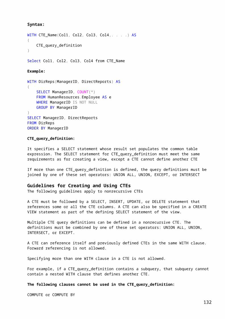
IF OBJECT_ID ( 'HumanResources.usp_GetEmployees2', 'P' ) IS NOT NULL DROP PROCEDURE HumanResources.usp_GetEmployees2;GOCREATE PROCEDURE HumanResources.usp_GetEmployees2 @lastname varchar(40) = 'D%', @firstname varchar(20) = '%'AS SELECT LastName, FirstName, JobTitle, Department FROM HumanResources.vEmployeeDepartment WHERE FirstName LIKE @firstname AND LastName LIKE @lastname;GO

You can Use any of the following command for different output:EXECUTE HumanResources.usp_GetEmployees2;-- OrEXECUTE HumanResources.usp_GetEmployees2 'Wi%';-- OrEXECUTE HumanResources.usp_GetEmployees2 @firstname = '%';-- OrEXECUTE HumanResources.usp_GetEmployees2 '[CK]ars[OE]n';-- OrEXECUTE HumanResources.usp_GetEmployees2 'Hesse', 'Stefen';-- OrEXECUTE HumanResources.usp_GetEmployees2 'H%', 'S%';

Using OUTPUT parameters

This procedures returns a list of products that have prices that do not exceed a specified amount. The example shows using multiple SELECT statements and multiple OUTPUT parameters. OUTPUT parameters enable an external procedure, a batch, or more than one Transact-SQL statement to access a value set during the procedure execution.

IF OBJECT_ID ( 'Production.usp_GetList', 'P' ) IS NOT NULL DROP PROCEDURE Production.usp_GetList;GOCREATE PROCEDURE Production.usp_GetList @product varchar(40) , @maxprice money , @compareprice money OUTPUT , @listprice money OUTAS SELECT p.name AS Product, p.ListPrice AS 'List Price' FROM Production.Product p JOIN Production.ProductSubcategory s ON p.ProductSubcategoryID = s.ProductSubcategoryID WHERE s.name LIKE @product AND p.ListPrice < @maxprice;-- Populate the output variable @listprice.SET @listprice = (SELECT MAX(p.ListPrice) FROM Production.Product p JOIN Production.ProductSubcategory s ON p.ProductSubcategoryID = s.ProductSubcategoryID WHERE s.name LIKE @product AND p.ListPrice < @maxprice);-- Populate the output variable @compareprice.SET @compareprice = @maxprice;

Execute usp_GetList to return a list of Adventure Works products (Bikes) that cost less than $700. The OUTPUT parameters @cost and @compareprices are used with control-of-flow language to return a message in the Messages window.

Note:

132

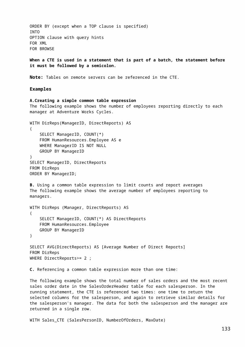
The OUTPUT variable must be defined when the procedure is created and also when the variable is used. The parameter name and variable name do not have to match; however, the data type and parameter positioning must match, unless @listprice = variable is used.

DECLARE @compareprice money, @cost money EXECUTE Production.usp_GetList '%Bikes%', 700, @compareprice OUT, @cost OUTIF @cost <= @compareprice BEGIN PRINT 'These products can be purchased for less than $'+RTRIM(CAST(@compareprice AS varchar(20)))+'.'ENDELSE PRINT 'The prices for all products in this category exceed $'+ RTRIM(CAST(@compareprice AS varchar(20)))+'.'

Using the WITH RECOMPILE option

The queries used by stored procedures are optimized only when they are compiled. As you make changes to the table structure or introduce new indexes which may optimize the data retrieval you should recompile your stored procedures as already compiled stored procedures may lose efficiency. By recompiling stored procedures you can optimize the queries. There are three ways in which you can force SQL Server to recompile your stored procedure: The sp_recompile system stored procedure forces a recompile of a stored procedure the next time it is executed.

IF OBJECT_ID ( 'dbo.usp_product_by_vendor', 'P' ) IS NOT NULL DROP PROCEDURE dbo.usp_product_by_vendor;GOCREATE PROCEDURE dbo.usp_product_by_vendor @name varchar(30) = '%'WITH RECOMPILEAS SELECT v.Name AS 'Vendor name', p.Name AS 'Product name' FROM Purchasing.Vendor v JOIN Purchasing.ProductVendor pv ON v.VendorID = pv.VendorID JOIN Production.Product p ON pv.ProductID = p.ProductID WHERE v.Name LIKE @name

Now Execute it

EXEC dbo.usp_product_by_vendor WITH RECOMPILE

Using ‘WITH ENCRYPTION’ OptionThe WITH ENCRYPTION option prevents the definition of the stored procedure from being returned, as shown by the following examples.

IF OBJECT_ID ( 'HumanResources.usp_encrypt_this', 'P' ) IS NOT NULL DROP PROCEDURE HumanResources.usp_encrypt_this;GOCREATE PROCEDURE HumanResources.usp_encrypt_thisWITH ENCRYPTIONAS SELECT EmployeeID, Title, NationalIDNumber, VacationHours, SickLeaveHours FROM HumanResources.Employee

Execute:

133

EXEC sp_helptext 'HumanResources.usp_encrypt_this'

Output would be:

The text for object 'HumanResources.usp_encrypt_this' is encrypted.

Note:Even DBA cannot see its code.Execute the following query against sys table. The first query shows code of procedure which is not encripted and second query shows null as it is encripted.

SELECT definition FROM sys.sql_modulesWHERE object_id = OBJECT_ID('HumanResources.usp_encrypt_this')

SELECT definition FROM sys.sql_modulesWHERE object_id = OBJECT_ID('HumanResources.usp_GetEmployees2')

To verify that the stored procedure has been created, run the following query:

SELECT definitionFROM sys.sql_modulesWHERE object_id = OBJECT_ID('dbo.usp_proc1')

Using the EXECUTE AS CALLER clause

The following example shows using the EXECUTE AS CALLER clause to specify the security context in which a stored procedure can be executed. In the example, the option CALLER specifies that the procedure can be executed in the context of the user that calls it.

IF OBJECT_ID ( 'Purchasing.usp_vendor_info_all', 'P' ) IS NOT NULL DROP PROCEDURE Purchasing.usp_vendor_info_all;GOCREATE PROCEDURE Purchasing.usp_vendor_info_allWITH EXECUTE AS CALLERAS SELECT v.Name AS Vendor, p.Name AS 'Product name', v.CreditRating AS 'Credit Rating', v.ActiveFlag AS Availability FROM Purchasing.Vendor v INNER JOIN Purchasing.ProductVendor pv ON v.VendorID = pv.VendorID INNER JOIN Production.Product p ON pv.ProductID = p.ProductID ORDER BY v.Name ASC

Error handling in SQL Server:

To handle Error in stored procedure, write the code in TRY block and error handling section in CATCH block.IF OBJECT_ID ( 'dbo.uspTryCatchTest', 'P' ) IS NOT NULL DROP PROCEDURE dbo.uspTryCatchTest;GOCREATE PROCEDURE uspTryCatchTestASBEGIN TRY SELECT 1/0END TRYBEGIN CATCH SELECT ERROR_NUMBER() AS ErrorNumber ,ERROR_SEVERITY() AS ErrorSeverity ,ERROR_STATE() AS ErrorState ,ERROR_PROCEDURE() AS ErrorProcedure ,ERROR_LINE() AS ErrorLine

134

,ERROR_MESSAGE() AS ErrorMessage;END CATCH

Dropping Stored Procedure:

DROP PROCEDURE uspGetAddressDropping multiple stored procedure in a single command

DROP PROCEDURE uspGetAddress, uspInsertAddress, uspDeleteAddress

ORDROP PROC uspGetAddress, uspInsertAddress, uspDeleteAddress

Modifying an Existing Stored ProcedureALTER PROCEDURE uspGetAddress @City nvarchar(30)ASSELECT * FROM Person.AddressWHERE City LIKE @City + '%'

You used to execute passing complete city name. Now pass the initial part of city name.Example:

exec uspGetAddress 'n'

Functions:

SQL Server user-defined functions are routines that accept parameters, perform an action, such as a complex calculation, and return the result of that action as a value. The return value can either be a single scalar value or a result set.

User-defined Function Benefits:

They allow modular programming. You can create the function once, store it in the database, and call it any

number of times in your program. User-defined functions can be modified independently of the program source code.

They allow faster execution. Similar to stored procedures, Transact-SQL user-defined functions reduce

the compilation cost of Transact-SQL code by caching the plans and reusing them for repeated executions. This means the user-defined function does not need to be reparsed and reoptimized with each use resulting in much faster execution times.

They can reduce network traffic.

Components of a User-defined Function:

All user-defined functions have the same two-part structure: a header and a body. The function takes zero or more input parameters and returns either a scalar value or a table.

The header defines:

Function name with optional schema/owner nameInput parameter name and data typeReturn parameter data type and optional name

The body defines the action, or logic, the function is to perform. It contains: One or more Transact-SQL statements that perform the function logic

135

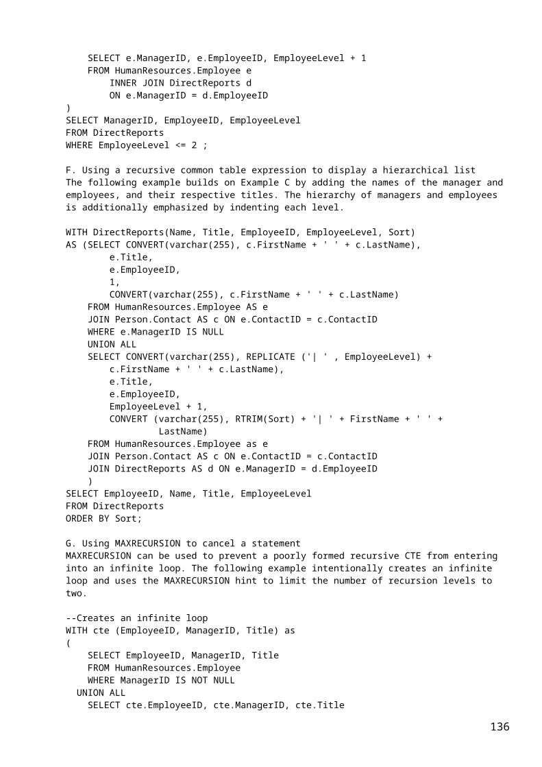
The following example shows a simple Transact-SQL user-defined. The function evaluates a supplied date, and returns a value designating the position of that date in a week.

CREATE FUNCTION dbo.GetWeekDay -- function name(@Date datetime) -- parameter name and data typeRETURNS int -- return value data typeASBEGIN -- begin body definitionRETURN DATEPART (weekday, @Date) -- performs the actionENDGO

The following example shows the function used in a Transact-SQL statement.

SELECT dbo.GetWeekDay(SalDate) AS DayOfWeek from sal

A user-defined function is stored as a database object providing reusable code that can be used in these ways:

In Transact-SQL (T-SQL) statements such as SELECT In applications calling the function In the definition of another user-defined function To parameterize a view or improve the functionality of an indexed view To define a column in a table To define a CHECK constraint on a column To replace a stored procedure

Choosing the Type of Function

When designing a user-defined function, first determine the type of function that is best suited to your needs. Will the function:

Return a scalar (single value) Return a table (multiple rows) Perform a complex calculation Primarily access SQL Server data

Types of functions:

Scalar Functions Table-Valued Functions

Scalar Functions

User defined scalar functions are of two types: Inline user-defined function Multistatement scalar function

Inline user-defined function

Inline user-defined functions are a subset of user-defined functions that return a table data type. Inline functions can be used to achieve the functionality of parameterized views.

Inline user-defined functions follow these rules:

The RETURNS clause contains only the keyword table. You do not have to define the format of a return variable, because it is set by the format of the result set of the SELECT statement in the RETURN clause.

There is no function_body delimited by BEGIN and END. The RETURN clause contains a single SELECT statement in parentheses. The

result set of the SELECT statement forms the table returned by the

136

function. The SELECT statement used in an inline function is subject to the same restrictions as SELECT statements used in views.

The table-valued function accepts only constants or @local_variable arguments

The following example returns store names and cities for a specified region:

USE AdventureWorks;GOCREATE FUNCTION Sales.ufn_CustomerNamesInRegion ( @Region nvarchar(50) )RETURNS tableASRETURN ( SELECT DISTINCT S.Name AS Store, A.City FROM Sales.Store AS S JOIN Sales.CustomerAddress AS CA ON CA.CustomerID = S.CustomerID JOIN Person.Address AS A ON A.AddressID = CA.AddressID JOIN Person.StateProvince SP ON SP.StateProvinceID = A.StateProvinceID WHERE SP.Name = @Region )GO

-- Example of calling the function for a specific region

SELECT *FROM Sales.ufn_CustomerNamesInRegion('Washington')GO

Multistatement scalar function:

User-defined scalar functions return a single data value of the type defined in the RETURNS clause. For an inline scalar function, there is no function body; the scalar value is the result of a single statement. For a multistatement scalar function, the function body, defined in a BEGIN...END block, contains a series of Transact-SQL statements that return the single value. The return type can be any data type except text, ntext, image, cursor, and timestamp.

The following examples creates a multistatement scalar function. The function takes one input value, a ProductID, and returns a single data value, the aggregated quantity of the specified product in inventory.

CREATE FUNCTION dbo.ufnGetStock(@ProductID int)RETURNS int AS -- Returns the stock level for the product.BEGIN DECLARE @ret int; SELECT @ret = SUM(p.Quantity) FROM Production.ProductInventory p WHERE p.ProductID = @ProductID AND p.LocationID = '6'; IF (@ret IS NULL) SET @ret = 0 RETURN @retEND;GO

The following example uses the ufnGetStock function to return the current inventory quantity for products that have an ProductModelID between 75 and 80.

USE AdventureWorks;GO

137

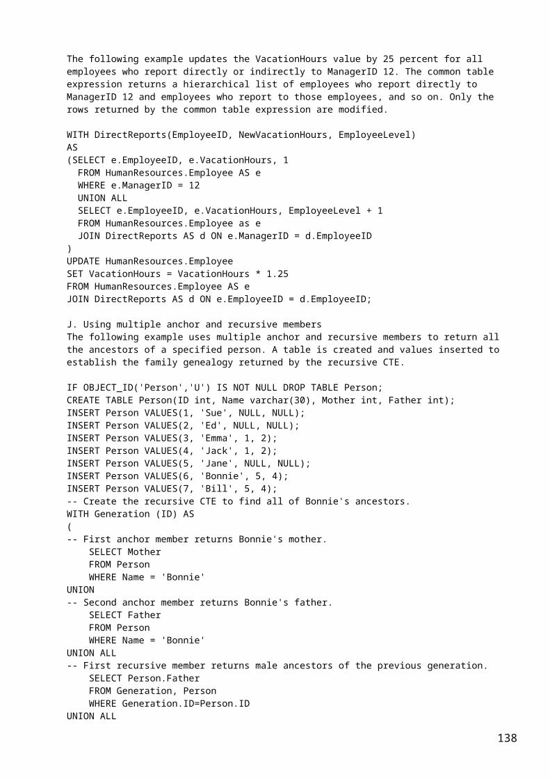
SELECT ProductModelID, Name, dbo.ufnGetStock(ProductID)AS CurrentSupplyFROM Production.ProductWHERE ProductModelID BETWEEN 75 and 80;GO

Table-Valued Functions

For a multistatement table-valued function, the function body, defined in a BEGIN...END block, contains a series of Transact-SQL statements that build and insert rows into the table that will be returned.

Components of a Table-Valued User-defined FunctionIn a table-valued user-defined function:

The RETURNS clause defines a local return variable name for the table returned by the function. The RETURNS clause also defines the format of the table. The scope of the local return variable name is local within the function.

The Transact-SQL statements in the function body build and insert rows into the return variable defined by the RETURNS clause.

When a RETURN statement is executed, the rows inserted into the variable are returned as the tabular output of the function. The RETURN statement cannot have an argument.

No Transact-SQL statements in a table-valued function can return a result set directly to a user. The only information the function can return to the user is the table returned by the function.

The following example creates a table-valued function. The function takes a single input parameter, an EmployeeID and returns a list of all the employees who report to the specified employee directly or indirectly.

USE AdventureWorks;GOCREATE FUNCTION dbo.fn_FindReports (@InEmpID INTEGER)RETURNS @retFindReports TABLE ( EmployeeID int primary key NOT NULL, Name nvarchar(255) NOT NULL, Title nvarchar(50) NOT NULL, EmployeeLevel int NOT NULL, Sort nvarchar (255) NOT NULL)--Returns a result set that lists all the employees who report to the --specific employee directly or indirectly.*/ASBEGIN WITH DirectReports(Name, Title, EmployeeID, EmployeeLevel, Sort) AS (SELECT CONVERT(Varchar(255), c.FirstName + ' ' + c.LastName), e.Title, e.EmployeeID, 1, CONVERT(Varchar(255), c.FirstName + ' ' + c.LastName) FROM HumanResources.Employee AS e JOIN Person.Contact AS c ON e.ContactID = c.ContactID WHERE e.EmployeeID = @InEmpID UNION ALL SELECT CONVERT(Varchar(255), REPLICATE ('| ' , EmployeeLevel) + c.FirstName + ' ' + c.LastName), e.Title, e.EmployeeID, EmployeeLevel + 1, CONVERT (Varchar(255), RTRIM(Sort) + '| ' + FirstName + ' ' + LastName) FROM HumanResources.Employee as e

138

JOIN Person.Contact AS c ON e.ContactID = c.ContactID JOIN DirectReports AS d ON e.ManagerID = d.EmployeeID )-- copy the required columns to the result of the function INSERT @retFindReports SELECT EmployeeID, Name, Title, EmployeeLevel, Sort FROM DirectReports RETURNEND;GO

In the following example, the above function is invoked.

-- Example invocationSELECT EmployeeID, Name, Title, EmployeeLevelFROM dbo.fn_FindReports(109)ORDER BY Sort;

NOTE:

User-defined functions that return a table data type can be powerful alternatives to views. These functions are referred to as table-valued functions. A table-valued user-defined function can be used where table or view expressions are allowed in Transact-SQL queries. While views are limited to a single SELECT statement, user-defined functions can contain additional statements that allow more powerful logic than is possible in views.

A table-valued user-defined function can also replace stored procedures that return a single result set. The table returned by a user-defined function can be referenced in the FROM clause of a Transact-SQL statement, but stored procedures that return result sets cannot.

In the following example, the table-valued function ufnGetContactInformation is invoked in two SELECT statements.

USE AdventureWorks;GOSELECT ContactID, FirstName, LastName, JobTitle, ContactTypeFROM dbo.ufnGetContactInformation(2200);GOSELECT ContactID, FirstName, LastName, JobTitle, ContactTypeFROM dbo.ufnGetContactInformation(5);GO

One more completed example:

The following example creates the ufnGetContactInformation function referenced in the example above and demonstrates the components of the table-valued function. In this function, the local return variable name is @retContactInformation. Statements in the function body insert rows into this variable to build the table result returned by the function.

USE AdventureWorks;GOCREATE FUNCTION dbo.ufnGetContactInformation(@ContactID int)RETURNS @retContactInformation TABLE ( -- Columns returned by the function ContactID int PRIMARY KEY NOT NULL, FirstName nvarchar(50) NULL, LastName nvarchar(50) NULL, JobTitle nvarchar(50) NULL, ContactType nvarchar(50) NULL)

139

AS -- Returns the first name, last name, job title and contact type for the specified contact.BEGIN DECLARE @FirstName nvarchar(50), @LastName nvarchar(50), @JobTitle nvarchar(50), @ContactType nvarchar(50); -- Get common contact information SELECT @ContactID = ContactID, @FirstName = FirstName, @LastName = LastName FROM Person.Contact WHERE ContactID = @ContactID; SELECT @JobTitle = CASE -- Check for employee WHEN EXISTS(SELECT * FROM HumanResources.Employee e WHERE e.ContactID = @ContactID) THEN (SELECT Title FROM HumanResources.Employee WHERE ContactID = @ContactID) -- Check for vendor WHEN EXISTS(SELECT * FROM Purchasing.VendorContact vc INNER JOIN Person.ContactType ct ON vc.ContactTypeID = ct.ContactTypeID WHERE vc.ContactID = @ContactID) THEN (SELECT ct.Name FROM Purchasing.VendorContact vc INNER JOIN Person.ContactType ct ON vc.ContactTypeID = ct.ContactTypeID WHERE vc.ContactID = @ContactID) -- Check for store WHEN EXISTS(SELECT * FROM Sales.StoreContact sc INNER JOIN Person.ContactType ct ON sc.ContactTypeID = ct.ContactTypeID WHERE sc.ContactID = @ContactID) THEN (SELECT ct.Name FROM Sales.StoreContact sc INNER JOIN Person.ContactType ct ON sc.ContactTypeID = ct.ContactTypeID WHERE ContactID = @ContactID) ELSE NULL END; SET @ContactType = CASE -- Check for employee WHEN EXISTS(SELECT * FROM HumanResources.Employee e WHERE e.ContactID = @ContactID) THEN 'Employee' -- Check for vendor WHEN EXISTS(SELECT * FROM Purchasing.VendorContact vc INNER JOIN Person.ContactType ct ON vc.ContactTypeID = ct.ContactTypeID WHERE vc.ContactID = @ContactID) THEN 'Vendor Contact' -- Check for store WHEN EXISTS(SELECT * FROM Sales.StoreContact sc INNER JOIN Person.ContactType ct ON sc.ContactTypeID = ct.ContactTypeID WHERE sc.ContactID = @ContactID) THEN 'Store Contact'

140

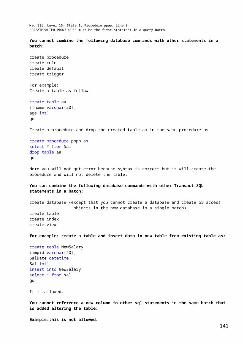
-- Check for individual consumer WHEN EXISTS(SELECT * FROM Sales.Individual i WHERE i.ContactID = @ContactID) THEN 'Consumer' END; -- Return the information to the caller IF @ContactID IS NOT NULL BEGIN INSERT @retContactInformation SELECT @ContactID, @FirstName, @LastName, @JobTitle, @ContactType; END; RETURN;END;GO

In the following example, the table-valued function ufnGetContactInformation is invoked in two SELECT statements by passing the contactId (fount in employee or contact table).SELECT ContactID, FirstName, LastName, JobTitle, ContactTypeFROM dbo.ufnGetContactInformation(1209)

Differences between stored procedure and functions in SQL Server:

A FUNCTION always returns a value using the return statement. A PROCEDURE may return one or more values through parameters or may not return at all.

Functions are normally used for computations where as procedures are normally used for executing business logic.

A Function returns 1 value only. Procedure can return multiple values (max 1024).

A Function can be used in the SQL Queries while a procedure cannot be used in SQL queries that cause a major difference b/w function and procedures.

Stored procedure can run independently. It can be executed using EXECUTE or EXEC command

The function cannot run independently. It has to be the part of the SQL statement.

Procedures can have input,output parameters for it whereas functions can have only input parameters.

The stored procedures can do all the DML operations like insert the new record, update the records and delete the existing records. But the function can do only select operation.

Triggers:

A trigger is a special kind of stored procedure that automatically executes when an event occurs in the database server.

DML triggers execute when a user tries to modify data through a data manipulation language (DML) event. DML events are INSERT, UPDATE, or DELETE statements on a table or view.

DDL triggers execute in response to a variety of data definition language (DDL) events. These are primarily CREATE, ALTER, and DROP statements. DML and DDL triggers can be created in the SQL Server 2005 Database Engine directly from Transact-SQL statements

In a RDBMS, a trigger is a SQL procedure that initiates an action (i.e. fires an action) when an event (INSERT, DELETE or UPDATE) occurs. Since triggers are event-driven specialized procedures, they are stored in and managed by the DBMS. A trigger cannot be called or executed; the DBMS automatically fires the trigger as a result of a data modification to the associated table. Triggers are used to maintain the referential integrity of data by changing the data in a systematic fashion.

141

Each trigger is attached to a single, specified table in the database. A trigger do not accept parameters or arguments (but may store affected-data in temporary tables)

Triggers can be viewed as similar to stored procedures in that both consist of procedural logic that is stored at the database level. Stored procedures, however, are not event-drive and are not attached to a specific table as triggers are. Stored procedures are explicitly executed by invoking a CALL to the procedure while triggers are implicitly executed. In addition, triggers can also execute stored procedures.

A trigger can also contain INSERT, UPDATE and DELETE logic within itself, so when the trigger is fired because of data modification it can also cause another data modification, thereby firing another trigger. A trigger that contains data modification logic within itself is called a nested trigger.

Triggers Compared to Constraints

Constraints and DML triggers each have benefits that make them useful in special situations. The primary benefit of DML triggers is that they can contain complex processing logic that uses Transact-SQL code. Therefore, DML triggers can support all of the functionality of constraints; however, DML triggers are not always the best method for a given feature.

Entity integrity should always be enforced at the lowest level by indexes that are part of PRIMARY KEY and UNIQUE constraints or are created independently of constraints. Domain integrity should be enforced through CHECK constraints, and referential integrity (RI) should be enforced through FOREIGN KEY constraints, assuming their features meet the functional needs of the application.

DML triggers are most useful when the features supported by constraints cannot meet the functional needs of the application.

For example: FOREIGN KEY constraints can validate a column value only with an exact match to a value in another column, unless the REFERENCES clause defines a cascading referential action.

Constraints can communicate about errors only through standardized system error messages. If your application requires, or can benefit from, customized messages and more complex error handling, you must use a trigger.

DML triggers can cascade changes through related tables in the database; however, these changes can be executed more efficiently through cascading referential integrity constraints.

DML triggers can disallow or roll back changes that violate referential integrity, thereby canceling the attempted data modification. Such a trigger might go into effect when you change a foreign key and the new value does not match its primary key. However, FOREIGN KEY constraints are usually used for this purpose.

If constraints exist on the trigger table, they are checked after the INSTEAD OF trigger execution but prior to the AFTER trigger execution. If the constraints are violated, the INSTEAD OF trigger actions are rolled back and the AFTER trigger is not executed.

SQL Server includes two general types of triggers: DML triggers and DDL triggers. DDL triggers are new to SQL Server 2005. These triggers are invoked when a data definition language (DDL) event takes place in the server or database.

DML Triggers:

DML triggers are invoked when a data manipulation language (DML) event takes place in the database. DML events include INSERT, UPDATE, or DELETE statements that modify data in a specified table or view. A DML trigger can query other tables and can include complex Transact-SQL statements. The trigger and the statement that fires it are treated as a single transaction, which can be rolled

142

back from within the trigger. If a severe error is detected (for example, insufficient disk space), the entire transaction automatically rolls back.

DML triggers are useful in these ways: Triggers can evaluate the state of a table before and after a data

modification and take actions based on that difference. Multiple DML triggers of the same type (INSERT, UPDATE, or DELETE) on a

table allow multiple, different actions to take place in response to the same modification statement.

Triggers are useful when the features supported by constraints cannot meet the functionality requirements of a database.

A Froeign key constraint does not allow to delete its parent record from master data but cannot stop to delete itself if it is not master data for other table.

A check constraint can validate a column value only against a logical expression or another column in the same table. But it cannot validate data against the column of another table. These limitations of constraints are fulfilled by triggers.

Types of DML Triggers:

AFTER Triggers INSTEAD OF Triggers CLR Triggers

AFTER Triggers:

AFTER triggers are executed after the action of the INSERT, UPDATE, or DELETE statement is performed. Specifying AFTER is the same as specifying FOR, which is the only option available in earlier versions of Microsoft SQL Server. AFTER triggers can be specified only on tables.

INSTEAD OF Triggers:

INSTEAD OF triggers are executed in place of the usual triggering action. INSTEAD OF triggers can also be defined on views with one or more base tables, where they can extend the types of updates a view can support.

CLR Triggers:

A CLR Trigger can be either an AFTER or INSTEAD OF trigger. A CLR trigger can also be a DDL trigger. Instead of executing a Transact-SQL stored procedure, a CLR trigger executes one or more methods written in managed code that are members of an assembly created in the .NET Framework and uploaded in SQL Server.

Implementing DML Triggers:

Before you create a DML trigger, consider that:

The CREATE TRIGGER statement must be the first statement in the batch. All other statements that follow in that batch are interpreted as part of the definition of the CREATE TRIGGER statement.

Permission to create DML triggers defaults to the table owner, who cannot transfer it to other users.

DML triggers are database objects, and their names must follow the rules for identifiers.

You can create a DML trigger only in the current database, although a DML trigger can reference objects outside of the current database.

A DML trigger cannot be created on a temporary or system table, although DML triggers can reference temporary tables. System tables should not be referenced; use the Information Schema Views instead.

143

INSTEAD OF DELETE and INSTEAD OF UPDATE triggers cannot be defined on a table that has a foreign key defined with a DELETE or UPDATE action.

Although a TRUNCATE TABLE statement is like a DELETE statement without a WHERE clause (it deletes all rows), it does not cause DELETE triggers to fire because the TRUNCATE TABLE statement is not logged.

The WRITETEXT statement does not cause the INSERT or UPDATE triggers to fire.

When you create a DML trigger, specify: The name. The table upon which the trigger is defined. When the trigger is to fire. The data modification statements that activate the trigger. Valid options

are INSERT, UPDATE, or DELETE.

Understanding DDL Triggers vs. DML Triggers

DDL triggers and DML triggers are used for different purposes. DML triggers operate on INSERT, UPDATE, and DELETE statements, and help to enforce business rules and extend data integrity when data is modified in tables or views.

DDL triggers operate on CREATE, ALTER, DROP, and other DDL statements. They are used to perform administrative tasks and enforce business rules that affect databases. They apply to all commands of a single type across a database, or across a server.

Use DDL triggers when you want to do the following: You want to prevent certain changes to your database schema. You want something to occur in the database in response to a change in your

database schema. You want to record changes or events in the database schema. DDL triggers fire only after the DDL statements that trigger them are run.

DDL triggers cannot be used as INSTEAD OF triggers.

Magic Tables:

Whenever a trogger fires in response to the Insert, Delete or update statement, two special tables are created. These are called inserted and deleted tables that are also called the magic tables. They are conceptual tables and structurally similar to the table on which the trigger is defined.

SQL Server 2005 automatically creates and manages these tables. You can use these temporary, memory-resident tables to test the effects of certain data modifications and to set conditions for DML trigger actions.

In DML triggers, the inserted and deleted tables are primarily used to perform the following:

Extend referential integrity between tables. Insert or update data in base tables underlying a view. Test for errors and take action based on the error. Find the difference between the state of a table before and after a data

modification and take actions based on that difference.

The deleted table stores copies of the affected rows during DELETE and UPDATE statements. During the execution of a DELETE or UPDATE statement, rows are deleted from the trigger table and transferred to the deleted table. The deleted table and the trigger table ordinarily have no rows in common.

The inserted table stores copies of the affected rows during INSERT and UPDATE statements. During an insert or update transaction, new rows are added at the

144

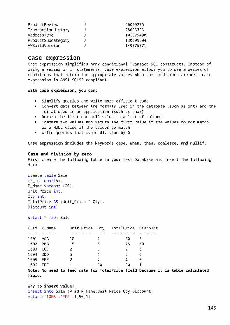
same time to both the inserted table and the trigger table. The rows in the inserted table are copies of the new rows in the trigger table.

An update transaction is similar to a delete operation followed by an insert operation; the old rows are copied to the deleted table first, and then the new rows are copied to the trigger table and to the inserted table.

Multiple DML Triggers:

A table can have multiple AFTER triggers of a given type provided they have different names; each trigger can perform numerous functions. However, each trigger can apply to only one table, although a single trigger can apply to any subset of three user actions (UPDATE, INSERT, and DELETE).

A table can have only one INSTEAD OF trigger of a given type.Trigger Limitations:

CREATE TRIGGER must be the first statement in the batch and can apply to only one table.

A trigger is created only in the current database; however, a trigger can reference objects outside the current database.

If the trigger schema name is specified to qualify the trigger, qualify the table name in the same way.

The same trigger action can be defined for more than one user action (for example, INSERT and UPDATE) in the same CREATE TRIGGER statement.

INSTEAD OF DELETE/UPDATE triggers cannot be defined on a table that has a foreign key with a cascade on DELETE/UPDATE action defined.

Note:

A TRUNCATE TABLE statement is not caught by a DELETE trigger. Although a TRUNCATE TABLE statement is, in effect, a DELETE without a WHERE clause because it removes all rows; it is not logged and therefore cannot execute a trigger. Because permission for the TRUNCATE TABLE belongs to the table owner and is not transferable, only the table owner should be concerned about inadvertently circumventing a DELETE trigger with a TRUNCATE TABLE statement.

The following Transact-SQL statements are not allowed in a DML trigger:

ALTER DATABASE CREATE DATABASEDROP DATABASE

LOAD DATABASE LOAD LOG RECONFIGURE

RESTORE DATABASERESTORE LOG  

DML Trigger syntax:

CREATE TRIGGER [ schema_name . ]trigger_name ON { table | view } { FOR | AFTER | INSTEAD OF } { [ INSERT ] [ , ] [ UPDATE ] [ , ] [ DELETE ] } AS { sql_statement}

DDL Trigger syntax:

CREATE TRIGGER trigger_name ON { ALL SERVER | DATABASE } { FOR | AFTER } { event_type | event_group } AS { sql_statement }

Alter DML Trigger syntax:

145

Alter TRIGGER [ schema_name . ]trigger_name ON { table | view } { FOR | AFTER | INSTEAD OF } { [ INSERT ] [ , ] [ UPDATE ] [ , ] [ DELETE ] } AS { sql_statement}

Alter DDL Trigger syntax:Alter TRIGGER trigger_name ON { ALL SERVER | DATABASE } { FOR | AFTER } { event_type | event_group } AS { sql_statement [ ; ] [ ...n ] | EXTERNAL NAME < method specifier > [ ; ] }

Dropping a DML trigger:

DROP TRIGGER schema_name.trigger_name

Dropping a DDL trigger:

DROP TRIGGER trigger_name ON { DATABASE | ALL SERVER }

Example of a simple DML Trigger:

Create trigger dbo.stopDMLon Dbo.MPRRFor Insert, update, deleteAS

BeginPrint 'DML Operation Not allowed'Rollback transaction

end

After creation this trigger, you cannot do DML Operation on MPRR table.

Try the following command:

delete from MPRR

select * from MPRR

Insert Trigger example:Insert Triggers fire when we attempt to insert a new record. If not restricted, a new record is inserted in both tables (Trigger table and inserted table)In an insert trigger, you can simply abort insert statement if inserting value is not correct with a message.

CREATE TRIGGER TrigInsertRequisition ON Requisition After INSERT AS

BEGIN Declare @VacancyReported int Declare @ActualVacancy int

select @ActualVacancy = BudgetedStrength-CurrentStrength from Position select @VacancyReported = inserted.NoOfVacancy from Inserted

IF (@VacancyReported > @ActualVacancy) Begin

Print 'The actual vacancies are less then reported vacancies hense unable to insert'

146

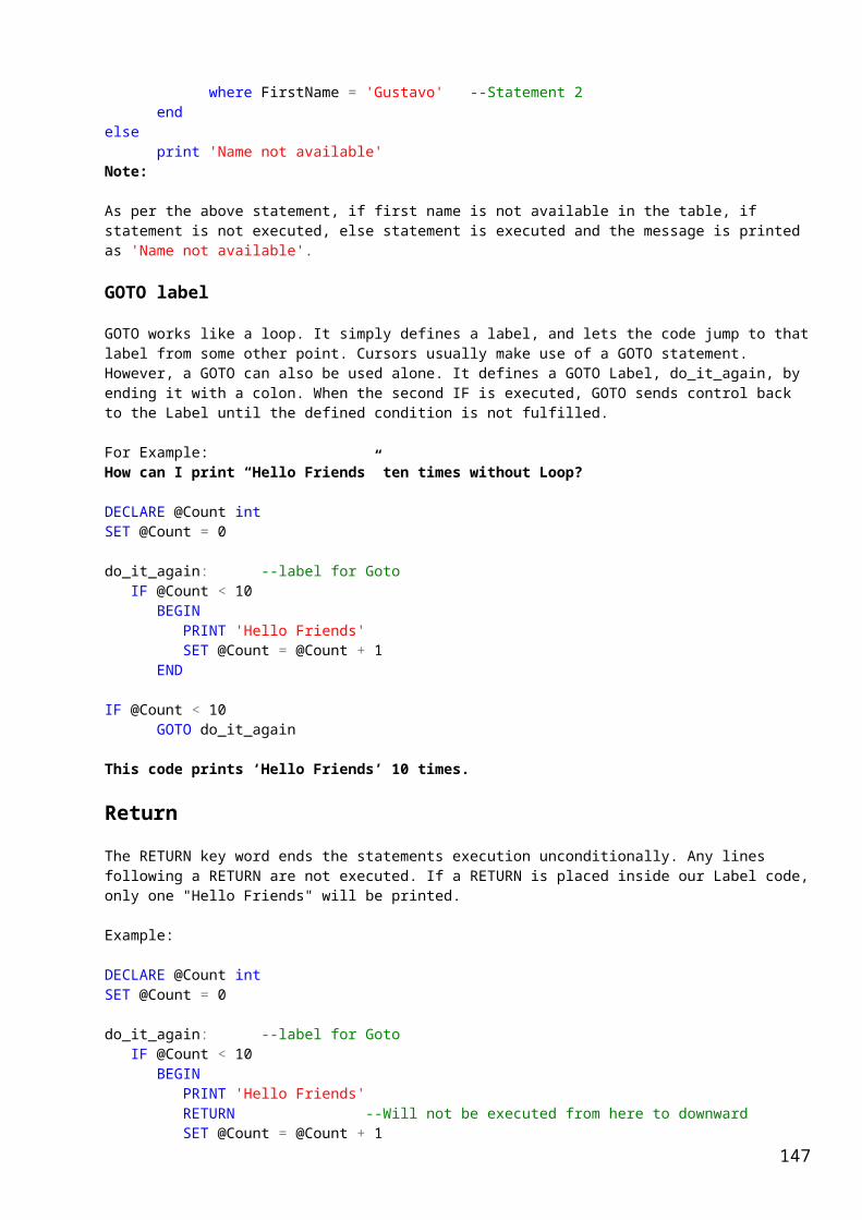
Rollback TransactionEnd

END

One More example:

CREATE TRIGGER mytrigger ON Sales INSTEAD OF INSERT AS BEGIN DECLARE @isnum TINYINT; SELECT @isnum = ISNUMERIC(Sale_Value) FROM inserted; IF (@isnum <1000) INSERT INTO Sales SELECT * FROM inserted; ELSE Print ‘SaleValue must be < 1000’ Rollback Transaction END

Delete trigger:

A delete trigger is used to prevent the illigal deletion. This trigger is fired when as attempt is made to delete a row from the trigger table if allowed. When a delete statement is issued, the specified rows are deleted from the table and are added to the deleted table. So The trigger table and deleted table do not have the common rows unlike insert trigger.

Example:

CREATE TRIGGER TrigDeletePub ON Publisher After Delete AS

BEGIN Declare @RowsDeleted int Declare @RowsLeft int Declare @RowsLeftChar char(10) Declare @MsgChar char(100)

select @RowsDeleted = (select count(*) from Deleted) select @RowsLeft = (select count(*) from from Publisher)

IF @RowsDeleted > @RowsLeftBegin

Select @RowsLeftChar=convert(varchar(10), @RowsLeft)Select @MsgChar='Only' + @RowsLeftChar + 'are left in Publisher'Print @MsgCharRollback Transaction

End END

Update trigger

When an update trigger is fired, it uses tow logical tables (inserted and deleted) to complete the operation. The deleted table contains the origional row and the inserted table contains the row with updated value.

147

Example:

CREATE TRIGGER TrigUpateItem ON Items For Update AS if update(Price)

beginprint 'you are not allowed to update price'Rollback Transaction

end

How to apply the business rules through trigger?

Suppose:

I want to keep my product table’s ‘quentity’ field with current value while I sell any product. For this I should create an insert trigger on orders table.

Example:First create a product table in your test database with following data:

create table product(prodId int,quantity int)

Data:

ProdId Quantity====== ========1 52 103 204 30

Create a table Orders

create table orders(ordId int,prodId int,quantity int)

Now create a trigger

CREATE TRIGGER TrigUpateProduct ON OrdersFor Insert AS

update Pset P.Quantity=(p.quantity-i.quantity)from product p join inserted ion p.prodId=i.prodId

Now insert a record into order as:

insert into Orders values(10,1,3)

select * from product

ProdId Quantity====== ========1 22 103 204 30

148

Instead Of Trigger For View:

********************************

Disable / Enable a DML or DDL trigger:

Syntax:

DISABLE TRIGGER { [ schema . ] trigger_name [ ,...n ] | ALL }ON { object_name | DATABASE | ALL SERVER } [ ; ]

Where:

ALL Indicates that all triggers defined at the scope of the ON clause are disabled.

object_name

Is the name of the table or view on which the DML trigger trigger_name was created to execute.

DATABASE

For a DDL trigger, indicates that trigger_name was created or modified to execute with database scope.

ALL SERVER

For a DDL trigger, indicates that trigger_name was created or modified to execute with server scope.

Note:

Triggers are enabled by default when they are created. Disabling a trigger does not drop it. The trigger still exists as an object in the current database. However, the trigger does not fire when any Transact-SQL statements on which it was programmed are executed. DML and DDL triggers can be re-enabled by using ENABLE TRIGGER. DML triggers defined on tables can be also be disabled or enabled by using ALTER TABLE.

Disabling a DML trigger on a table

The following example disables trigger uAddress that was created on table Address.

DISABLE TRIGGER Person.uAddress ON Person.Address

Disabling a DDL trigger

The following example creates a DDL trigger safety with database scope in your test Database.

CREATE TRIGGER safety ON DATABASE FOR DROP_TABLE, ALTER_TABLE AS PRINT 'You must disable Trigger "safety" to drop or alter tables!' ROLLBACK

Execute this and try to drop a table

149

drop table MPRR

output:

You must disable Trigger "safety" to drop or alter tables!Msg 3609, Level 16, State 2, Line 1The transaction ended in the trigger. The batch has been aborted.

To disable the trigger:

DISABLE TRIGGER safety ON DATABASE

Now try to drop the table as:

drop table MPRR

All Triggers of databse scope would be disabled and you can alter or drop table.

To re-enable trigger:

Enable TRIGGER safety ON DATABASE

If triggers are created on a table or a view:

ENABLE TRIGGER Person.uAddress ON Person.Address

Disabling all triggers that were defined with the same scopeThe following example disables all DDL triggers that were created at the server scope.

DISABLE Trigger ALL ON ALL SERVER

How to create database using T-SQL?

CREATE DATABASE MyTestDBONPRIMARY( NAME = MyTestDB_PrimaryDataFile, FILENAME = 'C:\SQLDatabases\MyTestDB_PrimaryDataFile.mdf' , SIZE = 3 MB , MAXSIZE = 10 MB , FILEGROWTH = 10 %),( NAME = MyTestDB_SecondaryDataFile, FILENAME = 'C:\SQLDatabases\MyTestDB_SecondaryDataFile.ndf' , SIZE = 1 MB , MAXSIZE = 10 MB , FILEGROWTH = 10 %),( NAME = MyTestDB_SecondaryDataFile2, FILENAME = 'C:\SQLDatabases\MyTestDB_SecondaryDataFile2.ndf' , SIZE = 1 MB , MAXSIZE = 10 MB , FILEGROWTH = 10 %)

LOG ON ( NAME = MyTestDB_LogFile, FILENAME = 'C:\SQLDatabases\MyTestDB_LogFile.ldf'

150

, SIZE = 2 MB , MAXSIZE = 15 MB , FILEGROWTH = 3 MB)COLLATE Latin1_General_CI_AS;

SSRS SSIS SSAS Locking and Transactions Query optimization, performance tunning, troubleshooting, use of Profiler, Query Plans, Partitioning DB object management via SQL scripting Logical and physical data modeling (ER tool) Database management basics concepts including Security and

SQL replication Backup and recovery Mirroring

151