Série Scientifique

Scientific Series

Nº 94s-23

HIGH-WAGE WORKERS

AND HIGH-WAGE FIRMS

John M. Abowd, Francis Kramarz,

David N. Margolis

Montréal

Décembre 1994

Ce document est publié dans l'intention de rendre accessible les résultats préliminaires de larecherche effectuée au CIRANO, afin de susciter des échanges et des suggestions. Les idées et lesopinions émises sont sous l'unique responsabilité des auteurs, et ne représentent pas nécessairementles positions du CIRANO ou de ses partenaires.This paper presents preliminary research carried out at CIRANO and aims to encourage

discussion and comment. The observations and viewpoints expressed are the sole responsibility

of the authors. They do not necessarily represent positions of CIRANO or its partners.

CIRANO

Le CIRANO est une corporation privée à but non lucratif constituée en vertu de la Loi

des compagnies du Québec. Le financement de son infrastructure et de ses activités

de recherche provient des cotisations de ses organisations-membres, d'une subvention

d'infrastructure du ministère de l'Industrie, du Commerce, de la Science et de la

Technologie, de même que des subventions et mandats obtenus par ses équipes de

recherche. La Série Scientifique est la réalisation d'une des missions que s'est données

le CIRANO, soit de développer l'analyse scientifique des organisations et des

comportements stratégiques.

CIRANO is a private non-profit organization incorporated under the Québec

Companies Act. Its infrastructure and research activities are funded through fees

paid by member organizations, an infrastructure grant from the Ministère de

l'Industrie, du Commerce, de la Science et de la Technologie, and grants and

research mandates obtained by its research teams. The Scientific Series fulfils one

of the missions of CIRANO: to develop the scientific analysis of organizations and

strategic behaviour.

Les organisations-partenaires / The Partner Organizations

�Ministère de l'Industrie, du Commerce, de la Science et de la Technologie.

�École des Hautes Études Commerciales.

�École Polytechnique.

�Université de Montréal.

�Université Laval.

�McGill University.

�Université du Québec à Montréal.

�Bell Québec.

�La Caisse de dépôt et de placement du Québec.

�Hydro-Québec.

�Banque Laurentienne du Canada.

�Fédération des caisses populaires de Montréal et de l'Ouest-du-Québec.

ISSN 1198-8177

The authors� affiliations are Cornell University, CREST-INSEE Department of Research and%

CIRANO-Université de Montréal, respectively. The authors gratefully acknowledge the financial andcomputing support of INSEE. Abowd and Margolis were also supported by the National ScienceFoundation (SBR 91-11186 and SBR\ 93-21053).We are grateful for the comments of David Card, RonaldEhrenberg, Hank Farber, Robert Gibbons, Guy Laroque, Stefan Lollivier, Bentley MacLeod, OliviaMitchell, Ariel Pakes, Alain Trognon and Martin Wells as well as for comments received during seminarsfar too numerous to mention here. The data used in this paper are confidential but the authors� access is notexclusive. Other researchers interested in using these data should contact the Centre de Recherche enEconomie et Statistique, ENSAE, 15 bd Gabriel Péri, 92244 Malakoff Cédex, France.

High-Wage Workers

and High-Wage Firms

John M. Abowd

Francis Kramarz

David N. Margolis%

Résumé / Abstract

Westudy a longitudinal sample of over one million French workers and over 500,000

employing firms. Real total annual compensation per worker is decomposed into components

related to observable characteristics, worker heterogeneity, firm heterogeneity and residual

variation. Except for the residual, all components may be correlated in an arbitrary fashion.

At the level of the individual, we find that person-effects, especially those not related to

observables like education, are a very important source of wage variation in France.

Firm-effects, while important, are not as important as person-effects. At the level of firms, we

find that enterprises that hire high-wage workers are more productive but not more

profitable. They are also more capital and high-skilled employee intensive. Enterprises that

pay higher wages, controlling for person-effects, are more productive and more profitable.

They are also more capital intensive but are not more high-skilled labor intensive. We also

find that person-effects explain 97% of inter-industry wage differentials.

Nous étudions un échantillon de données longitudinales sur plus de un million detravailleurs français à l�emploi de plus de 500 000 entreprises. La rémunération annuelle totalepar travailleur, en chiffres réels, est divisée en composantes reliées aux caractéristiquesobservables, à l�hétérogénéité des travailleurs, à l�hétérogénéité des entreprises et à la variationrésiduelle. À l�exception du résidu, toutes les composantes peuvent être corrélées de façonarbitraire. Sur le plan des travailleurs, nous trouvons que les effets individuels, notamment leseffets reliés à des caractéristiques observables comme le niveau d�études, sont une source trèsimportante de dispersion des salaires en France. Les effets propres à l�entreprise, même s�ils sontimportants, ne sont pas aussi importants que les effets individuels. Sur le plan des entreprises,nous trouvons que les entreprises qui embauchent des travailleurs à salaire élevé sont plusproductives mais non plus rentables. Elles se caractérisent également comme des entreprises àforte intensité de capital et en travailleurs hautement qualifiés. Les entreprises qui paient dessalaires plus élevés, compte tenu des effets individuels, sont plus productives et plus rentables.Elles ont aussi une plus forte intensité en capital, mais n�utilisent pas proportionnellement plusde travailleurs hautement qualifiés. Nous trouvons enfin que les effets individuels expliquent97 pour cent des différences de salaires entre industries.

1 Introduction

For several decades labor economists have lamented the lack of microeconomicdata relating characteristics of �rms to characteristics of their workers (see, forexample, Rosen (1986) and Willis (1986)) because such data would permit re-searchers to begin to disentangle the e�ects of �rm-level human resource policiesfrom the e�ects of external choices made by individual workers. Why do high-compensation �rms pay more than the apparent going wage? Perhaps such astrategy delivers a gain in productivity or pro�tability that exceeds the incre-mental wage cost, as predicted by e�ciency wage and agency models.1 Perhapshigh-paying �rms select workers with higher external wage rates, thus sortingthe workers into �rms that have di�erential observed compensation programs.2

Although broadly representative linked surveys of �rms and workers are notavailable in the U.S., there have now been numerous studies that attempt torelate �rm performance to the design of the compensation system. In this paperwe present the �rst extensive statistical analysis of the individual and �rm het-erogeneity in compensation determination. We examine variation in personalwage rates holding �rm-e�ects constant and variation in �rm wage rates holdingpersonal e�ects constant. Due to the longitudinal nature of our data, we areable to control for both measured and unmeasured heterogeneity in the workersand their employing �rms.

A high-wage worker is a person with total compensation higher than ex-pected on the basis of observable characteristics like labor force experience,education, region, or sex. A high-wage �rm is an employer with compensationhigher than expected given these same observable characteristics. Until nowall empirical analyses of personal and �rm heterogeneity in compensation out-comes have relied upon data that were inadequate to identify separately theindividual-e�ect necessary to classify a worker as high-wage and the �rm-e�ectrequired to classify a �rm as high-wage. Using a unique longitudinal data seton �rms and workers that is representative of private French employment, weare able to estimate both components of compensation determination, allowingfor unrestricted correlation among them. In the estimated models, we �nd thatindividual-e�ects are statistically more important than �rm-e�ects and that thetwo are not strongly correlated; however, the economic interpretation of thesestatements is complicated by the mobility patterns in the data. Although ourstatistical model allows for the identi�cation of both �rm- and individual-e�ects,we show that for many simple economic models, the structural heterogeneityof the workers and employers is not identical to the statistical heterogeneity

1See Lazear (1979), Shapiro and Stiglitz (1984), Hart and H�olmstrom (1987) and Sapping-

ton (1991) for concise statements of the theories generating these predictions. Tests of thesemodels have been performed by Abowd (1990), Abowd and Kramarz (1993), Gibbons andMurphy (1990, 1992) and Hutchens (1987).

2This view is espoused by Bulow and Summers (1976), Cain (1976), Jovanovic (1979),

and Roy (1951). Some tests of these models include Dickens and Lang (1985), Flinn (1986),Heckman and Sedlacek (1985).

1

measured by our descriptive model.We use the results of our individual-level data analysis to relate �rm-level

outcomes and choices to the structure of the �rm's compensation policy. Specif-ically, we ask whether �rms that hire high-wage workers are more pro�table(no), more productive per worker (yes), more capital intensive (yes), moreprofessional-employment intensive (yes), more skilled labor intensive (no) andmore likely to survive (yes). Second, we ask whether high-wage �rms are morepro�table (yes), more productive per worker (yes), more capital intensive (yes),more professional-employment intensive (no), more skilled labor intensive (no)and more likely to survive (maybe). Finally, we aggregate our results to theindustry level, where we �nd that high-wage workers and high-wage �rms areboth explanations of the inter-industry wage di�erential with high-wage workersbeing much more important empirically.

The paper is organized as follows. Section 2 describes our analysis data set.Section 3 describes our methods for identifying and estimating the large numberof statistical e�ects that characterize worker and �rm compensation heterogene-ity and provides several potential economic interpretations of the descriptivemodel's parameters. Section 4 describes our results. Section 5 concludes. AData Appendix describes our manipulation of the French data in great detail.Finally, a Model Appendix gives details of the theoretical calculations.

2 Data Description and Sampling Plans

Our sample of workers comes from the D�eclarations Annuelles de Salaires (DAS),an annual survey of employer-reported earnings subject to French social securitytaxes. We follow approximately one million individuals over the years from 1976to 1987. The sample is a 1/25th extract of the French work force, excluding gov-ernment employees (but including employees of government-owned businesses).Our compensation measure is the real total annual compensation cost for theemployee. This includes direct salary and all bene�t costs.3 The data sourcereports the number of days worked per year. Part time workers were excluded.The total compensation measure for part year workers was annualized on a baseof 360 days per year. The data included the individual's age, sex, location ofjob, occupation, and an identi�er for the employer. We supplemented thesedata with information on the individual's education, available for ten percentof the sample and imputed for the rest (see the Data Appendix). We followedworkers and employers across years and assigned a worker to the employer forwhich he or she had the largest number of paid days in a given year. We referto the resulting analysis data �le as the \individual data."

Our sample of �rms comes from the annual survey B�en�e�ces Industrielset Commerciaux (BIC), which collects a large amount of income statement,

3Some components of employer compensation costs were estimated by the Revenus divisionat INSEE.

2

balance sheet, employment and ow of funds information in support of theFrench national accounts. We use a probability sample of 20,000 of these �rms,followed from 1978 to 1988, constructed by INSEE to facilitate research on�rms (INSEE, 1989, 1990a-1990c). Our measures of �rm performance includevalue added per employee, operating income as a proportion of total assetsand sales per employee. As measures of factor inputs we calculated total realassets and total year-end employment. We added detailed measures of the�rm's employment structure (professional, skilled and unskilled) from the annualEnquete sur la Structure des Emplois (Survey of employment structure). Werefer to the resulting analysis data �le as the \�rm data."

The worker and �rm samples are linked using an identi�cation number(SIREN) for the employer that corresponds to a business unit{one or moreestablishments engaged in a related economic activity. Thus, our analysis of�rm-e�ects is at the level of an enterprise and not at the level of establishments.We do not use the ownership structure of our �rms. When the enterpriseschange owners but remain in the same business, their SIRENs do not normallychange. Thus, we are able to follow the economic activity of our �rms throughmost �nancial and ownership restructurations. We use the linked individual-�rm data to estimate the relation among various compensation policies and�rm-level economic variables.

3 A Statistical Model for Individual Compensa-

tion

The basic compensation equation for an individual is given by

yit = xit� + �i + J(i;t)it + "it (1)

where yit is the compensation of individual i = 1; :::; N , for time t = Fi; :::; Li, Fiis the �rst year an individual appears in the data, Li is the last year s/he appearsin the sample, and the function J(i; t) gives the identity j of the employing �rmfor individual i at date t. The e�ect xit� is the predicted e�ect of time varying,person-speci�c characteristics xit with � being a vector of parameters to beestimated. The time-invariant individual-e�ect �i is decomposed as

�i = �i + ui� (2)

where ui is a vector of observable time-invariant person-speci�c characteristicsand � is a vector of parameters to be estimated. The �rm-e�ect J(i;t)it isdecomposed as

J(i;t)it = �J(i;t) + 1J(i;t)sJ(i;t)it + 2 J(i;t)T1(sJ(i;t)it � 10) (3)

where �J(i;t), 1J(i;t) and 2J(i;t) are �rm-speci�c parameters to be estimated,sJ(i;t)it is individual i's seniority at date t in �rm J(i; t) and the function T1(z)

3

is the linear spline basis function

T1(z) =

�0 for z < 0z for z � 0

�:4 (4)

Finally, the error term "it is stochastically independent of all other e�ects inequation (1) with E["it] = 0 and Var["it] = �2" . The stochastic structure of xit�,�i and J(i;t)it is unrestricted so that these e�ects may be cross-correlated. Theidenti�cation conditions imposed upon the model areX

i

�i = 0

and Xi;t

J(i;t)it = 0:

3.1 Potential Interpretations of the Descriptive Model

We illustrate the relation between structural heterogeneity in the populations ofworkers (heterogeneous abilities or tastes) and �rms (heterogeneous e�cienciesor technologies) and the statistical heterogeneity in equation (1) using threeeconomic models with very simple population structures. In each case we derivethe conditional expectation of individual compensation given the identity ofthe employing �rm and the individual. We then relate the parameters of thisconditional expectation to our statistical parameterization above.

3.1.1 A matching model with endogenous turnover

Suppose that workers are homogeneous. There are two types of �rms, m andn, and two periods. In type m �rms a worker's marginal product and wagerate are always w�, and employment is always available in a type m �rm. Intype n �rms there is a matching process. Worker i's productivity is w� +"in in both periods with "in drawn from a binomial distribution B(�H;H; 1

2).

The matching outcome, "in, unknown to both the worker and the �rm at thebeginning of the �rst period of employment, is realized at the end of the �rstperiod and becomes public information. Workers are o�ered contracts at thebeginning of the �rst period of the form (w1; w2) and workers may leave �rmn at the end of the �rst period. All �rms make zero pro�ts. The equilibriumcontract for �rms of type n is (w� � H

2; w� + "in). All workers in type n �rms

with a bad matching outcome (�H) quit to type m �rms.

4The use of a linear spline at 10 years of seniority is a speci�cation that we found bettersuited to these data than a quadratic. As will become evident below, three parameters at the�rm level is already quite exible and we did not �nd much to be gained by adding additionpolynomial tems in seniority.

4

To simplify the model, we consider a stationary situation with nine workerswho live for two periods each, three born in period 0, three born in period 1,three born in period 2. Two workers in each generation enter type n �rms, oneworker in each generation enters a type m �rm. Of the two workers who enteredtype n �rms, let one draw a positive matching outcome and the other draw anegative matching outcome. The worker with the negative matching outcomeleaves the type n �rm for a type m �rm when the matching parameter is madepublic.

The structure of the data implied by this theoretical model is shown inappendix Table B1. This corresponds to the following parameter values in ourdescriptive model:

� = w�

where � is the overall mean;

�i = 0; i = 1; :::; 9

where �i is person i person-e�ect;

(�m; m) = (0; 0)

for the type m �rm compensation policy; and

(�n; n) = (�H

2;3H

2)

for the type n �rm compensation policy.

3.1.2 A rent-splitting model with exogenous turnover

Suppose there are four di�erent individuals, two types of �rms, m and n, andtwo time periods. Each of the two �rms earns quasi-rents of qjt, and the quasi-rents are split by negotiation so that the workers receive a share sj of thequasi-rent in �rm j. Suppose that each �rm employs two workers. With proba-bility one, exactly one worker is randomly selected to separate from the periodone employer and be re-employed at the other �rm in the second period. Allinformation about the workers and �rms is known to those parties but not tothe statistician. All workers are included in the data sample and the typicalworker has wages of the form:

yit = xi + sjqjt

where xj is the measure of wage rate heterogeneity, i.e. the worker type, qjtfollows a binomial distribution B(�Q;Q; 1

2), i = 1:::; 4, j = m;n, and t = 1; 2.

Table B2 shows the relation among the theoretical parameters, xi, sj , and Q,and the statistical parameters of equation (1) for each worker and each period.The model cannot be solved exactly. Thus, we use these relations to solve, by

5

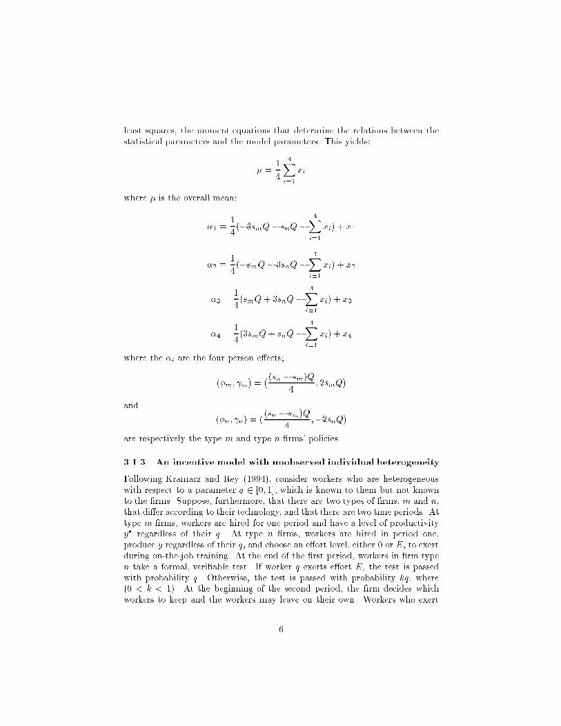
least squares, the moment equations that determine the relations between thestatistical parameters and the model parameters. This yields:

� =1

4

4Xi=1

xi

where � is the overall mean;

�1 =1

4(�3smQ� snQ �

4Xi=1

xi) + x1

�2 =1

4(�smQ� 3snQ �

4Xi=1

xi) + x2

�3 =1

4(smQ+ 3snQ�

4Xi=1

xi) + x3

�4 =1

4(3smQ+ snQ�

4Xi=1

xi) + x4

where the �i are the four person e�ects;

(�m; m) = ((sn � sm)Q

4; 2smQ)

and

(�n; n) = ((sn � sm)Q

4;�2snQ)

are respectively the type m and type n �rms' policies.

3.1.3 An incentive model with unobserved individual heterogeneity

Following Kramarz and Rey (1994), consider workers who are heterogeneouswith respect to a parameter q 2 [0; 1], which is known to them but not knownto the �rms. Suppose, furthermore, that there are two types of �rms, m and n,that di�er according to their technology, and that there are two time periods. Attype m �rms, workers are hired for one period and have a level of productivityy� regardless of their q. At type n �rms, workers are hired in period one,produce y regardless of their q, and choose an e�ort level, either 0 or E, to exertduring on-the-job training. At the end of the �rst period, workers in �rm typen take a formal, veri�able test. If worker q exerts e�ort E, the test is passedwith probability q. Otherwise, the test is passed with probability kq, where(0 < k < 1). At the beginning of the second period, the �rm decides whichworkers to keep and the workers may leave on their own. Workers who exert

6

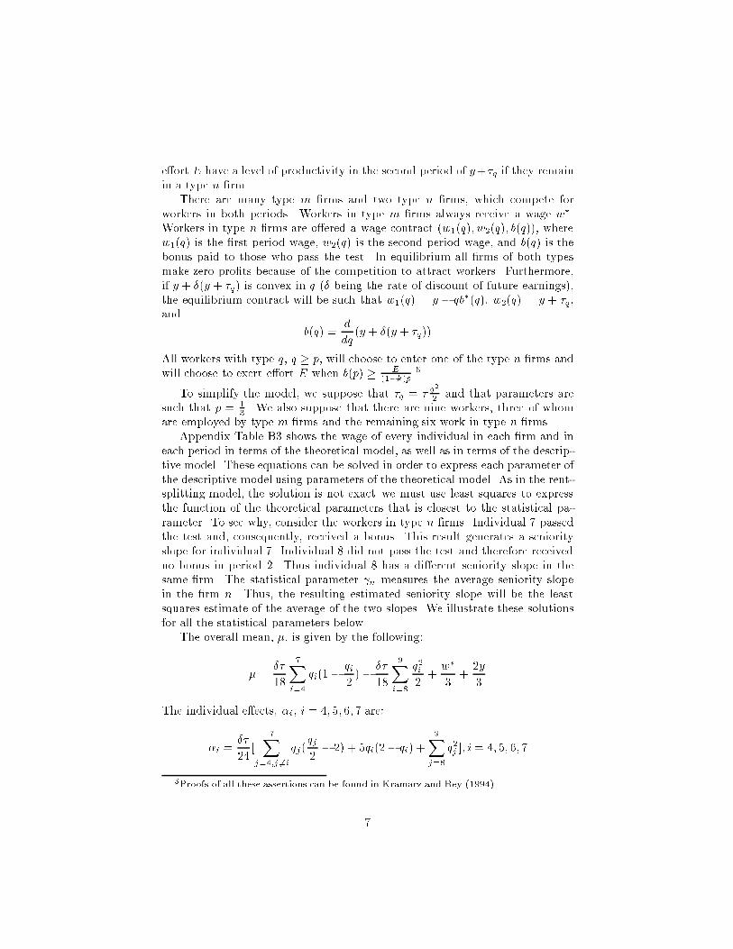
e�ort E have a level of productivity in the second period of y+�q if they remainin a type n �rm.

There are many type m �rms and two type n �rms, which compete forworkers in both periods. Workers in type m �rms always receive a wage w�.Workers in type n �rms are o�ered a wage contract (w1(q); w2(q); b(q)), wherew1(q) is the �rst period wage, w2(q) is the second period wage, and b(q) is thebonus paid to those who pass the test. In equilibrium all �rms of both typesmake zero pro�ts because of the competition to attract workers. Furthermore,if y + �(y + �q) is convex in q (� being the rate of discount of future earnings),the equilibrium contract will be such that w1(q) = y � qb�(q), w2(q) = y + �q,and

b(q) =d

dq(y + �(y + �q))

All workers with type q, q � p, will choose to enter one of the type n �rms andwill choose to exert e�ort E when b(p) � E

(1�k)p .5

To simplify the model, we suppose that �q = �q2

2and that parameters are

such that p = 13. We also suppose that there are nine workers, three of whom

are employed by type m �rms and the remaining six work in type n �rms.Appendix Table B3 shows the wage of every individual in each �rm and in

each period in terms of the theoretical model, as well as in terms of the descrip-tive model. These equations can be solved in order to express each parameter ofthe descriptive model using parameters of the theoretical model. As in the rent-splitting model, the solution is not exact{we must use least squares to expressthe function of the theoretical parameters that is closest to the statistical pa-rameter. To see why, consider the workers in type n �rms. Individual 7 passedthe test and, consequently, received a bonus. This result generates a seniorityslope for individual 7. Individual 8 did not pass the test and therefore receivedno bonus in period 2. Thus individual 8 has a di�erent seniority slope in thesame �rm. The statistical parameter n measures the average seniority slopein the �rm n. Thus, the resulting estimated seniority slope will be the leastsquares estimate of the average of the two slopes. We illustrate these solutionsfor all the statistical parameters below.

The overall mean, �, is given by the following:

� =��

18

7Xi=4

qi(1�qi

2) �

��

18

9Xi=8

q2i2+w�

3+

2y

3

The individual e�ects, �i, i = 4; 5; 6; 7 are:

�i =��

24[

7Xj=4;j 6=i

qj(qj

2� 2) + 5qi(2� qi) +

9Xj=8

q2j ]; i = 4; 5; 6; 7

5Proofs of all these assertions can be found in Kramarz and Rey (1994).

7

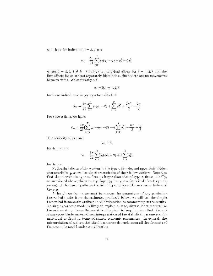
and those for individual i = 8; 9 are:

�i =��

24[7X

j=4

qj(qj � 2) + q2k � 5q2i ]

where k = 8; 9, i 6= k. Finally, the individual e�ects for i = 1; 2; 3 and the�rm e�ects for m are not separately identi�able, since there are no movementsbetween �rms. We arbitrarily set:

�i = 0; i = 1; 2; 3

for these individuals, implying a �rm e�ect of:

�m =��

36[7Xi=4

qi(qi � 2) +9Xi=8

q2i ] +2w�

3�

2y

3

For type n �rms we have:

�n =��

36[

7Xi=4

qi(�5qi � 2)� 59Xi=8

q2i ]�w�

3+y

3:

The seniority slopes are: m = 0

for �rm m and

n =��

12[7Xi=4

qi(3qi + 2) + 39Xi=8

q2i ]

for �rm n.Notice that the �i of the workers in the type n �rm depend upon their hidden

characteristics qi as well as the characteristics of their fellow workers. Note alsothat the intercept in type m �rms is larger than that of type n �rms. Finally,as mentioned above, the seniority slope, n, in type n �rms is the least squaresaverage of the career paths in the �rm, depending on the success or failure ofthe test.

Although we do not attempt to recover the parameters of any particulartheoretical model from the estimates produced below, we will use the simpletheoretical frameworks outlined in this subsection to comment upon the results.No single economic model is likely to explain a large, diverse labor market likethe one we study. Nevertheless, it is important to keep in mind that it is notalways possible to make a direct interpretation of the statistical parameters (forindividual or �rm) in terms of simple economic parameters. In general, theinterpretation of a given statistical parameter depends upon all the elements ofthe economic model under consideration.

8

3.2 Computation and Identi�cation in the Statistical Model

In the context of equation (1), our goal is to estimate the invariant parame-ters � and � consistently in the presence of individual- and �rm-e�ects thatmay be correlated with the person-speci�c characteristics. Next, we want toestimate �i and J(i;t)it in a manner that allows us to use these estimates,when averaged within a �rm j, as potential explanatory variables for di�er-ences in �rm productivity, pro�tability, factor utilization and survival. Thecomputational problem we face is that the least squares design matrix impliedby equations (2) and (3) is enormous and cannot be simpli�ed using any ofthe standard techniques in linear models (as, for example, in Sche�e, 1959).There are over one million individuals and 500,000 �rms (of which 14,000 haveat least 10 individual-year observations) represented in our data. Thus, elim-inating the individual-e�ects from (1) by deviations from person-means leavesa high dimension, non-sparse, non-patterned least squares equation system tosolve for the time-invariant and �rm-speci�c parameters. Similarly, eliminatingthe �rm-e�ects by deviations from �rm-means (conditional on seniority) leavesan equally complex least squares equation system to solve. Finally, adoptingChamberlain's (1984) method of projecting the individual- and �rm-e�ects ontoa set of person and �rm characteristics, while permitting consistent estimationof � and �, complicates our second goal by forcing us to model the �rm-levele�ects of compensation policies directly in (1).

We adopt a variant of Chamberlain's method with a simpli�cation �rst pro-posed by Mundlak (1978). In our projection method we project the �rm-e�ectonto a vector of �rm and person characteristics constructed so as to allow thedesired correlation among the individual-e�ects, observable individual charac-teristics and the �rm-e�ects. This permits consistent estimation of � and leastsquares estimation of �i. The resulting estimates are then used to produceconsistent estimates of the �rm-e�ects and of the �rm-level averages of theindividual-e�ects, which we use in our �rm-level analysis.

It is worth discussing why we rejected two potential computational simpli�cations{sampling individuals and sampling �rms{thus reducing the dimensionality of theperson- and �rm-e�ects to make the problem tractable. The person e�ects aretypically identi�ed by repeated observations on the same individual and the �rme�ects are typically identi�ed by multiple employees in the same �rm. Whenboth types of e�ect are present in the same model, �rm-e�ects are identi�edby the presence in the sample of individuals observed for multiple years andin multiple �rms that employ other members of the sample. Without somemovement of the individuals among the �rms, neither �rm- nor person-e�ectsare separately identi�able. However, a relatively small amount of mobility suf-�ces to identify many �rm- and person-e�ects. The identi�cation of the personand �rm e�ects for individuals with at least two observations occurs wheneverthese individuals work at least once in a �rm that has at some point employeda person who changed employers. When sampling individuals, as the size of the

9

sample increases, the representativeness of the estimated �rm-e�ects improvesbecause in small samples of individuals the identi�ed �rm-e�ects are mostlyfrom large �rms, whereas in larger samples the additional individuals increasethe probability that there will be a mover among the smaller �rms. Further-more, reducing the size of the individual sample would have prevented us fromestimating �rm-speci�c seniority returns because there are fewer and fewer �rmswith adequate sample sizes as the sample of individuals is reduced. On the otherhand, when sampling �rms we can estimate only selected �rm-e�ects using allthe available individual observations, assuming that the �rm-e�ects from thenonsampled �rms are zero. To obtain a representative, reasonably large setof �rm-e�ect estimates, this procedure would have to be repeated many times(approximately 1,000 times to reproduce the �rm-e�ects we have estimated byour preferred method). It is not obvious that this procedure o�ers any compu-tational advantages.

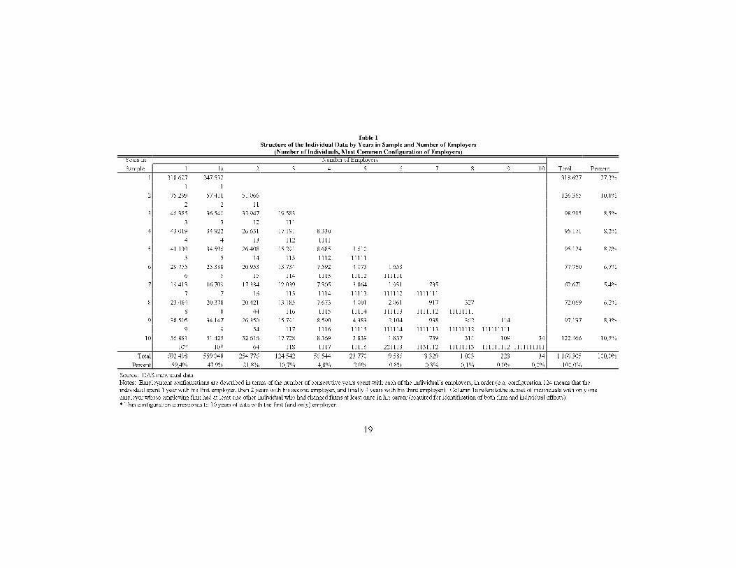
Regardless of the computational approach used, between-employer mobil-ity of the individuals is essential for the identi�cation of our statistical model.Table 1 examines the pattern of inter-employer movements among all sampleindividuals. The rows of Table 1 correspond to the number of years a person isin the sample. The columns, with the exception of column (1a), correspond tothe number of employers the individual had. An individual contributes to onlyone cell (again, excepting column (1a)). Notice that 59.4% of the individuals inthe sample never change employers (column (1)).6 Approximately one-�fth ofthe single employer individuals worked in �rms with no movers while four-�fths(47.9% of the overall sample, column (1a)) worked in �rms that, at one time oranother, employed a person who changed employer. Thus, 88.5% of the sampleindividuals contribute to the estimation of �rm-e�ects. It is also interesting tonotice the pattern of employer spells among the movers (columns (2)-(10)). Thesecond line of each cell shows the most frequent con�guration of employer spellsfor individuals in that cell. In almost every case, short spells precede longerspells, indicating that mobility is greater in the early career (as Topel and Ward(1992) found for American men). It seems clear from Table 1 that the datashould allow us to separate the individual-e�ect from the �rm-e�ect.

3.3 A Projection Method for Estimating Correlated Ef-

fects

Our proposed method allows us to estimate the parameters � consistently inthe presence of both individual- and �rm-e�ects without adopting a step-wiseapproach that imposes orthogonality among the di�erent e�ects. We project

6Notice that the cell (1,1) contains 318,627 individuals who appear in the sample during

a single year. Some of these individuals may represent coding errors in the person identi�er;however, it is not possible to correct these errors.

10

the �rm-e�ect onto the �rm and individual data according to the equation:

�J(i;t) + 1 J(i;t)sJ(i;t)it + 2 J(i;t)T1(sJ(i;t)it � 10) =�fJ(i;t)t

�1 sJ(i;t)it T1(sJ(i;t)it � 10)

� xi

�� + �J(i;t)it (5)

where fJ(i;t)t is a vector of time varying �rm characteristics (�rm size in ourapplication), xi is the vector of person-averages of xit:

xi �1

Ti

LiXt=Fi

xit (6)

Ti � Li � Fi + 1, � is the parameter vector of the linear projection and �J(i;t)itis the stochastic error of the linear projection. Let

zit ��fJ(i;t)t

�1 sJ(i;t)it T1(sJ(i;t)it� 10)

� xi

�(7)

thenyit = xit� + zit� + �i + "it + �J(i;t)it: (8)

Restated as deviations from individual-averages, equation (8) becomes

eyit = exit� + ezit�+ e"it + e�J(i;t)it (9)

where exit � xit � xi (10)

and similarly for ezit; e"it and e�J(i;t)it. Least squares estimation of � and � yields:

" b�b�#! N

��

�

�; �21

" eX0 eX eX0 eZeZ0 eX eZ0 eZ#�1 !

as N !1 (11)

where

eX �

2666666664

ex11:::ex1T1:::exN1

:::ex1TN

3777777775; eZ �

2666666664

ez11:::ez1T1:::ezN1

:::ez1TN

3777777775

and �21 � Varhe"it + e�J(i;t)it j eX; eZi .

Estimates of the individual e�ects �i are recovered in the conventional manneras b�i = yit � xib� � zib� (12)

11

and the limit distribution of b�i isb�i ! N

�i;�xi zi

�Var

" b�b�# �

x0iz0i

�+�21Ti

!as N !1 (13)

We note that although the least squares estimate of the individual e�ect b�i isnot consistent as N ! 1, this is not a problem when we estimate �rm-levelmodels because the �rm-average of b�i can be consistently estimated.

Next consider the estimation of the �rm e�ects �J(i;t) + 1 J(i;t)sJ(i;t)it + 2J(i;t) T1(sJ(i;t)it - 10). De�ne

fjg � f(i; t) j J(i; t) = jg , a set with Nj elements, (14)

byfjg � yfjg � xfjgb� � b�fjg; (15)

yfjg �

24 :::

yns:::

35 ; 8(n; s) 2 fjg ; (16)

and similarly for xfjg and �fjg. Equations (14) and (15) group all of the obser-vations on individuals employed by the same �rm into the vector byfjg, whichis expressed as a deviation from the x� e�ects and the individual e�ects. The�rm-level equation is:

byfjg = Ffjg

24 �j 1j 2j

35+ &fjg (17)

where

Ffjg �

24 :::

1 sns T1(sns � 10):::

35 ; 8(n; s) 2 fjg (18)

and&fjg � "fjg + xfjg

�� � b��+ ��fjg � b�fjg� (19)

Least squares estimation of (17) yields the estimator24 b�jb 1jb 2j

35! N

0@24 �j 1j 2j

35 ;j

1A as Nj !1 (20)

where

j � �22

�F 0fjgFfjg

��1

+�F 0fjgFfjg

��1

F 0fjg�

Xfjg

Varhb�iX0

fjg+Var

hb�fjg

i+ 2X

fjgCov

hb�; b�fjg

i�Ffjg

�F 0fjgFfjg

��1

(21)

12

and �22 = Var [&].To recover the �i and ui� parts of the individual e�ect, estimate the equation

(2) by generalized least squares to obtain b�, which satis�es:

b� ! N

�;

�U 0Diag

�Var

hb�ii��1

U

��1!as N !1 (22)

where

U �

24 u1

:::

uN

35 (23)

and Diag�Var

hb�ii�is a diagonal matrix containing the variances of b�i fromequation (13). The estimator of �i is

b�i = b�i � uib� (24)

and

b�i ! N

�i;

�21Ti

"1�

Ti

�21u0i

�U 0Diag

�Var

hb�ii��1

U

��1

ui

#!, as N !1

(25)Next we estimate the �rm-level average �i; de�ned as �j,

b�j � 1

Nj

X8(i;t)2fjg

b�i (26)

with asymptotic distribution:

b�j ! N��j; �

2�j

�, as Nj !1 (27)

where

�2�j �1

N2j

NjXi=1

�21Ti

"1�

Ti

�21u0i

�U 0Diag

�Var

hb�ii��1

U

��1

ui

#:

Similarly, the �rm-level average education e�ect is given by

ujb� � 1

Nj

X8(i;t)2fjg

uib� (28)

with asymptotic distribution based upon (22).7

7In all our asymptotic results we hold constant the distribution of �rm sizes. Thus asN;Nj !1;we assume that their ratio goes to a non-zero constant.

13

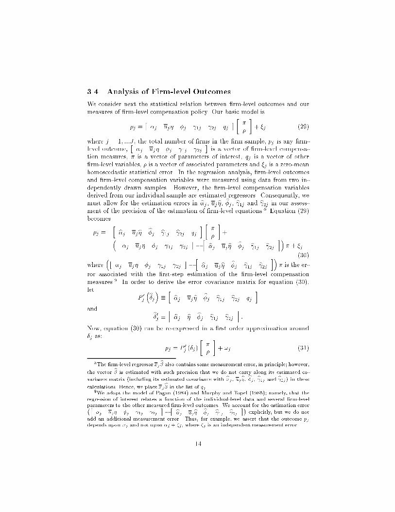
3.4 Analysis of Firm-level Outcomes

We consider next the statistical relation between �rm-level outcomes and ourmeasures of �rm-level compensation policy. Our basic model is

pj =��j uj� �j 1j 2j qj

� � ��

�+ �j (29)

where j = 1; :::J , the total number of �rms in the �rm sample, pj is any �rm-level outcome,

��j uj� �j 1j 2j

�is a vector of �rm-level compensa-

tion measures, � is a vector of parameters of interest, qj is a vector of other�rm-level variables, � is a vector of associated parameters and �j is a zero-meanhomoscedastic statistical error. In the regression analysis, �rm-level outcomesand �rm-level compensation variables were measured using data from two in-dependently drawn samples. However, the �rm-level compensation variablesderived from our individual sample are estimated regressors. Consequently, wemust allow for the estimation errors in b�j; ujb�; b�j; b 1j and b 2j in our assess-ment of the precision of the estimation of �rm-level equations.8 Equation (29)becomes

pj =h b�j ujb� b�j b 1j b 2j qj

i ��

�

�+��

�j uj� �j 1j 2j��h b�j ujb� b�j b 1j b 2j i�� + �j

(30)

where��

�j uj� �j 1j 2j��h b�j ujb� b�j b 1j b 2j i�� is the er-

ror associated with the �rst-step estimation of the �rm-level compensationmeasures.9 In order to derive the error covariance matrix for equation (30),let

P 0j

�b�j� � h b�j ujb� b�j b 1j b 2j qj

iand b�0j � h b�j b� b�j b 1j b 2j i :Now, equation (30) can be re-expressed in a �rst order approximation around�j as:

pj = P 0j (�j)

��

�

�+ !j (31)

8The �rm-level regressor xjb� also contains some measurement error, in principle; however,

the vector b� is estimated with such precision that we do not carry along its estimated co-

variance matrix (including its estimated covariance with b�j; ujb�; b�j; b 1j and b 2j) in these

calculations. Hence, we place xjb� in the list of qj.9We adopt the model of Pagan (1984) and Murphy and Topel (1985); namely, that the

regression of interest relates a function of the individual-level data and several �rm-levelparameters to the other measured �rm-level outcomes. We account for the estimation error��

�j uj� �j 1j 2j

��

� b�j ujb� b�j b 1j b 2j �� explicitly, but we do not

add an additional measurement error. Thus, for example, we assert that the outcome pjdepends upon �j and not upon �j + �j, where �j is an independent measurement error.

14

where

!j � (b�j � �j)0@Pj (�j)

@�j

��

�

�+ �j

The variance of the regression error term for equation (31) consists of the com-

ponent due to the estimation error in bPj plus the component due to �j:

Var [!j ] ���0 �0

� @P 0j

@�0jVar

hb�ji @Pj@�j

��

�

�+ Var [�j] (32)

where the components of Varhb�ji are de�ned in the derivations above. We

estimate equation (31) using generalized least squares based upon the errorvariance in equation (32).

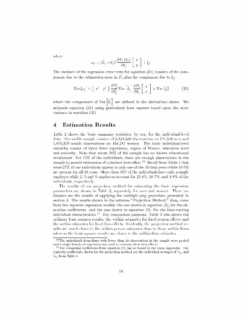
4 Estimation Results

Table 2 shows the basic summary statistics, by sex, for the individual-leveldata. The usable sample consists of 3,434,530 observations on 711,518 men and1,870,578 usable observations on 454,787 women. The basic individual-levelvariables consist of labor force experience, region of France, education leveland seniority. Note that about 30% of the sample has no known educationalattainment. For 74% of the individuals, there are enough observations in thesample to permit estimation of a distinct �rm-e�ect.10 Recall from Table 1 thatsome 27% of our individuals appear in only one of the 10 data years while 10.6%are present for all 10 years. More than 59% of the individuals have only a singleemployer while 2, 3 and 4 employers account for 21.8%, 10.7%, and 4.8% of theindividuals, respectively.

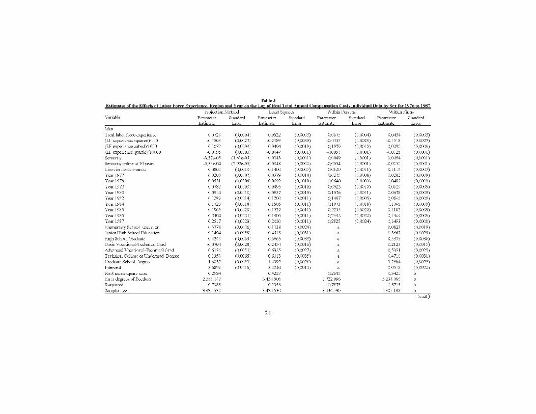
The results of our projection method for estimating the basic regressionparameters are shown in Table 3, separately for men and women. These es-timates are the results of applying the multiple step procedure presented insection 3. The results shown in the columns "Projection Method," thus, comefrom two separate regression models{the one shown in equation (2), for the ed-ucation coe�cients, and the one shown in equation (9), for the time-varyingindividual characteristics.11 For comparison purposes, Table 3 also shows theordinary least squares results, the within estimates for �xed person-e�ects andthe within estimates for �xed �rm-e�ects. Evidently, the projection method re-sults are much closer to the within-person estimates than to those within �rmswhereas the least squares results are closer to the within-�rm estimates.

10The individuals from �rms with fewer than 10 observations in the sample were pooledand a single �rm-level regression was used to estimate their �rm-e�ects.

11The remaining coe�cients from equation (9) can be found in the Data Appendix. Theseniority coe�cients shown for the projection method are the individual averages of b 1j andb 2j from Table 4.

15

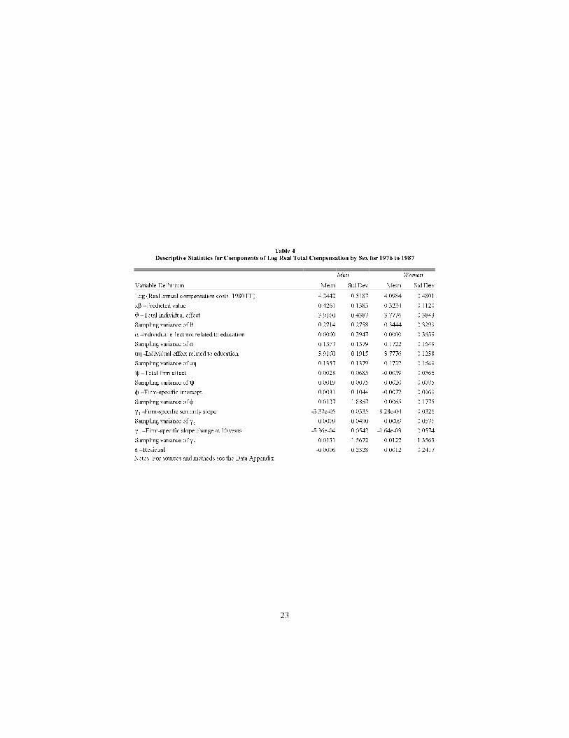
Table 4 contains descriptive statistics for the components of real compensa-tion implied by the estimated parameters from equation (1) separately for eachsex. For both males and females, the standard deviation of the individual-e�ect,and its components �and u�, is much larger than that of the �rm-e�ect, and itscomponents �, 1 and 2. As noted in Table 3, the complete parameterizationin explains 80% of the variation in real salaries for men and 75% for women;thus, the idiosyncratic component of variance is still rather important.

Table 5 shows the intercorrelations of the components of compensation. Allcomponents of compensation except the residual account for 81% of the vari-ance of real total annual compensation costs (combined result for males andfemales). Furthermore, the �i component of the individual-e�ect (the part notexplained by education) is more important than the observable regressors (x�)in explaining compensation costs. The overall �rm e�ect, j, on the otherhand, is only about one-quarter as important as the overall person-e�ect. Theindividual-e�ect and the �rm-e�ect are correlated 0.10 according to our results.The � and � components are correlated 0.08 according to this method. Noticethat although the �rm-speci�c intercept, �, and the �-component of the indi-vidual e�ect are positively correlated, the �rm-speci�c intercept is negativelycorrelated with the seniority slope (-0.56).

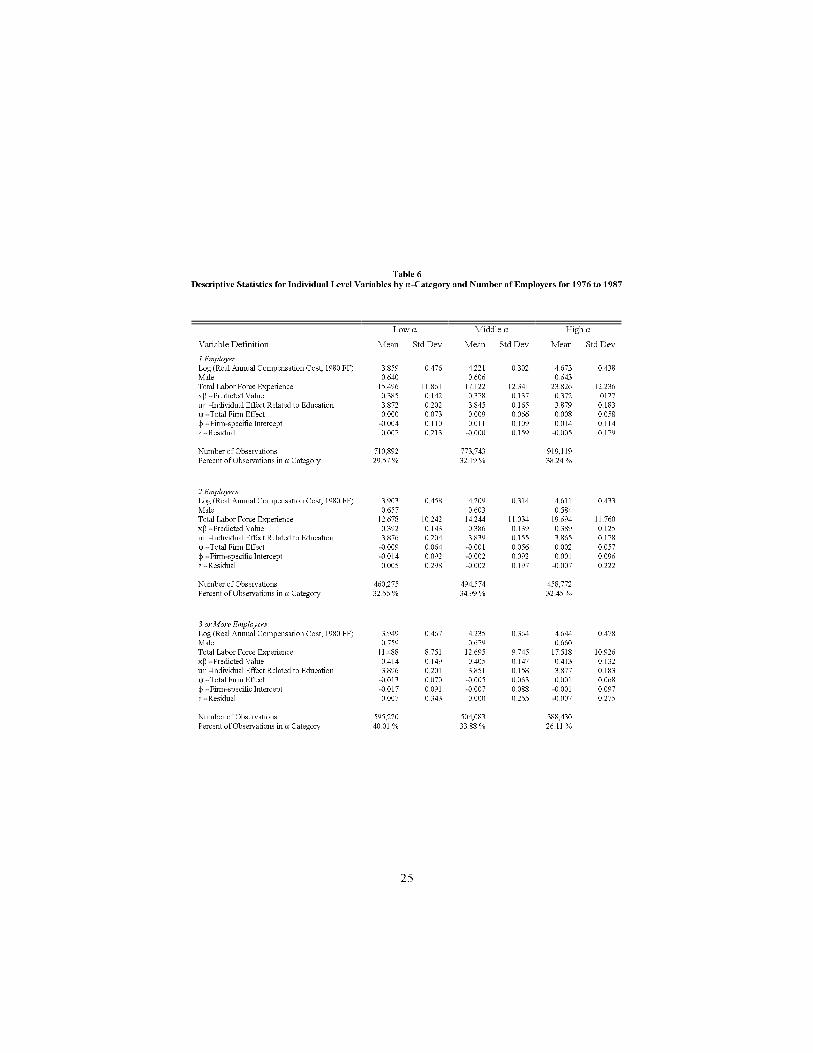
One may get the impression from Table5 that the individual-e�ects and�rm-e�ects are not highly correlated. Table 6 shows that this is not completelycorrect. In this table we begin to address the problem of inter-employer mobilityin our sample. If the mobility in the economy is exogenous; that is, if theprobability of separation from one �rm and accession into another does notdepend upon the individual's wage path, then the association of the parameter�j with the pay practices of �rm j is correct. Otherwise, the movers and stayerssystematically sort according to their values of �, �, and ". In this secondcase, measured values of �rm-e�ects are contaminated by the average values ofindividual-e�ects of the movers relative to the stayers, as can be seen in the twoendogenous mobility models discussed above.

For Table 6, the individuals were divided into three groups according totheir �'s. High-� workers are much more likely to be observed in a singlejob (one employer) whereas low-� workers are relatively more likely to have hadthree or more employers. High-� workers also have more labor-force experience.Although � and � are positively correlated, low-�workers are more likely to havehad multiple employers. In particular the low-� low-� low experience workersare the most likely to have had multiple employers. Table 7 examines themobility of high-� versus low-� workers explicitly. Persons with low estimatedindividual-e�ects are much more likely to move between low-� jobs than arepersons with high individual-e�ects (57% versus 40%). Evidently the cleandistinction between individual heterogeneity and �rm heterogeneity is calledinto question by this pattern. Do we estimate low �'s because the individualhas moved through a sequence of low-� jobs or rather because some employersare more likely to choose low-� workers, who are more mobile for a variety of

16

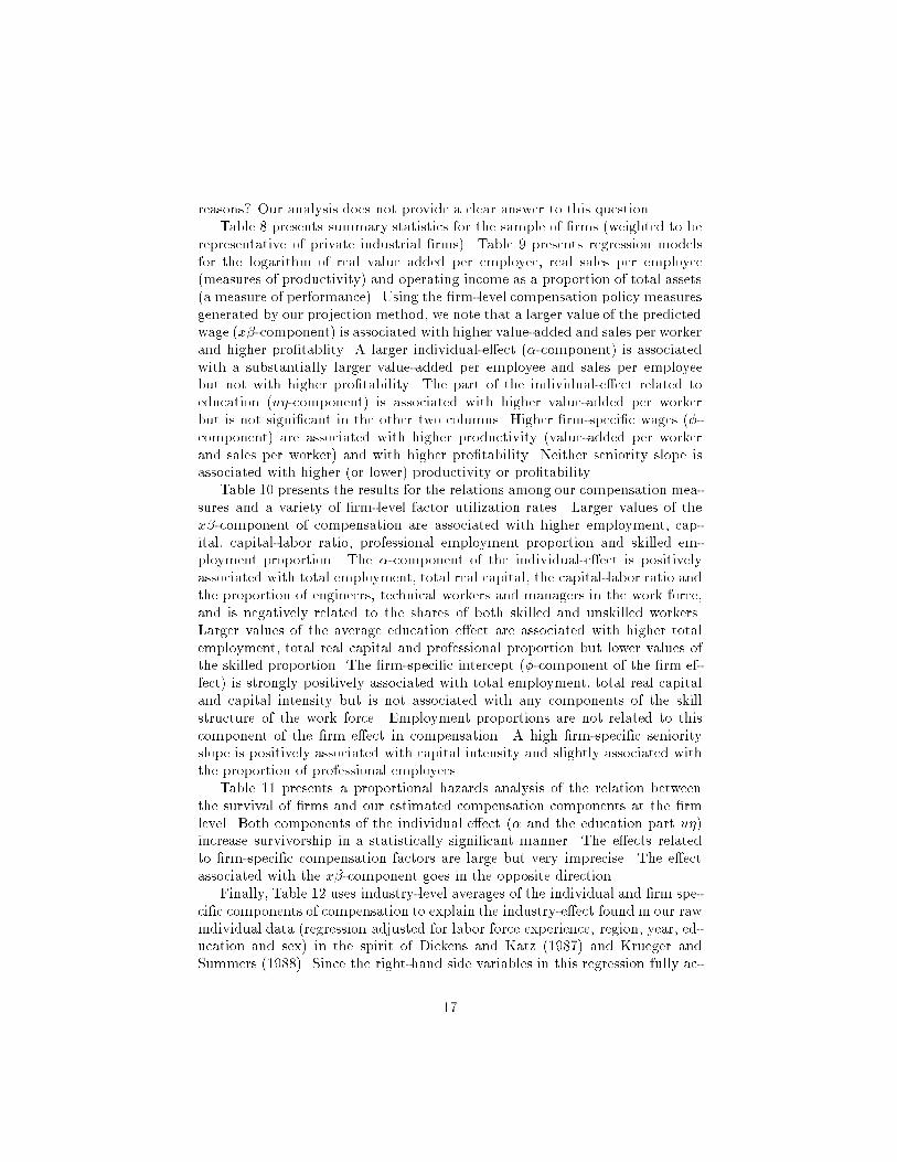
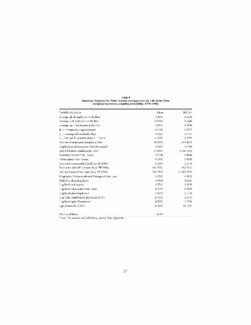
reasons? Our analysis does not provide a clear answer to this question.Table 8 presents summary statistics for the sample of �rms (weighted to be

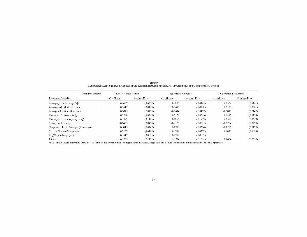
representative of private industrial �rms). Table 9 presents regression modelsfor the logarithm of real value added per employee, real sales per employee(measures of productivity) and operating income as a proportion of total assets(a measure of performance). Using the �rm-level compensation policy measuresgenerated by our projection method, we note that a larger value of the predictedwage (x�-component) is associated with higher value-added and sales per workerand higher pro�tablity. A larger individual-e�ect (�-component) is associatedwith a substantially larger value-added per employee and sales per employeebut not with higher pro�tability. The part of the individual-e�ect related toeducation (u�-component) is associated with higher value-added per workerbut is not signi�cant in the other two columns. Higher �rm-speci�c wages (�-component) are associated with higher productivity (value-added per workerand sales per worker) and with higher pro�tability. Neither seniority slope isassociated with higher (or lower) productivity or pro�tability.

Table 10 presents the results for the relations among our compensation mea-sures and a variety of �rm-level factor utilization rates. Larger values of thex�-component of compensation are associated with higher employment, cap-ital, capital-labor ratio, professional employment proportion and skilled em-ployment proportion. The �-component of the individual-e�ect is positivelyassociated with total employment, total real capital, the capital-labor ratio andthe proportion of engineers, technical workers and managers in the work force,and is negatively related to the shares of both skilled and unskilled workers.Larger values of the average education e�ect are associated with higher totalemployment, total real capital and professional proportion but lower values ofthe skilled proportion. The �rm-speci�c intercept (�-component of the �rm ef-fect) is strongly positively associated with total employment, total real capitaland capital intensity but is not associated with any components of the skillstructure of the work force. Employment proportions are not related to thiscomponent of the �rm e�ect in compensation. A high �rm-speci�c seniorityslope is positively associated with capital intensity and slightly associated withthe proportion of professional employees.

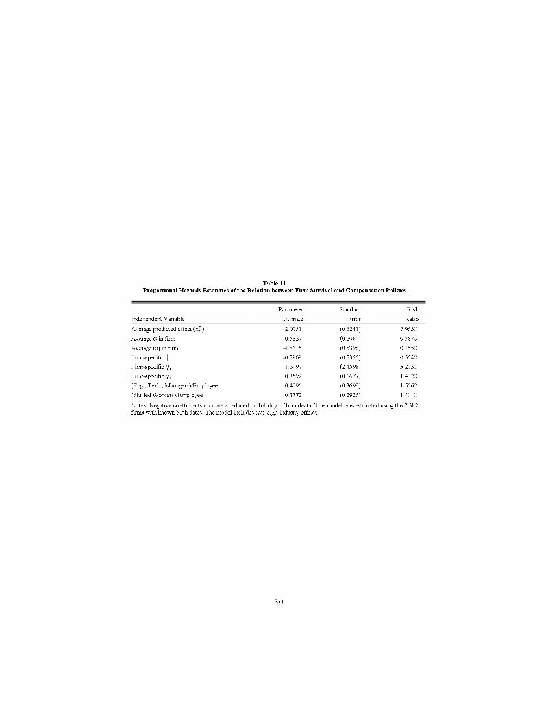
Table 11 presents a proportional hazards analysis of the relation betweenthe survival of �rms and our estimated compensation components at the �rmlevel. Both components of the individual e�ect (� and the education part u�)increase survivorship in a statistically signi�cant manner. The e�ects relatedto �rm-speci�c compensation factors are large but very imprecise. The e�ectassociated with the x�-component goes in the opposite direction.

Finally, Table 12 uses industry-level averages of the individual and �rm spe-ci�c components of compensation to explain the industry-e�ect found in our rawindividual data (regression adjusted for labor force experience, region, year, ed-ucation and sex) in the spirit of Dickens and Katz (1987) and Krueger andSummers (1988). Since the right-hand side variables in this regression fully ac-

17

count for the industry e�ects in a statistical sense (R2 = 0:97), the interestingquestion is the relative importance of individual heterogeneity (�-component ofthe person e�ect) and �rm heterogeneity (both � and -components) as com-ponents of the industry e�ects. The third through sixth columns of Table 12present separate industry-level regressions using �rst � alone (column 3 and 4)and then the three parts of the �rm-e�ect by themselves (columns 5 and 6).It is clear from the fact that � alone explains 92% of the inter-industry wagevariation, whereas the �rm-speci�c components explain only 25%, that individ-ual e�ects, as measured statistically are more important than �rm-components.One should recall, however, that in our example theoretical models structural�rm and individual heterogeneity can in uence both of the statistical measures.

5 Conclusions

In all likelihood, our analysis of the separate e�ects of individual and �rm het-erogeneity on wage rates and on �rm compensation policies has raised morenew questions than it has resolved. We �nd that individual-e�ects are a signi�-cant component of real total annual compensation variation. Firm-e�ects, whilealso important, are not as important as individual-e�ects. Firm-level hetero-geneity and individual-level heterogeneity are not highly correlated; however,mobility patterns suggest that the distinction between an individual-e�ect anda �rm-e�ect is not economically simple. Firms that hire high-wage workersappear to be more productive per worker but not more pro�table. High-wage�rms{those paying higher wages controlling for the individual heterogeneity ofthe employees{are more productive per worker and are more pro�table. Bothsources of wage rate heterogeneity{high-wage workers and high-wage �rms{areassociated with more capital intensive �rms. We also estimated �rm-level het-erogeneity in the returns to seniority. This component of wage variation is decid-edly less important in our sample than the two pure heterogeneity components.We believe that our results provide the statistical basis upon which to beginthe process of testing the relevance of agency, e�ciency wage, search/matching,and endogeneous mobility models as potential explanations for compensationoutcome heterogeneity.

18

19

Table 1

Structure of the Individual Data by Years in Sample and Number of Employers

(Number of Individuals, Most Common Configuration of Employers)

Years in Number of Employers

Sample 1 1a 2 3 4 5 6 7 8 9 10 Total Percent

1 318.627 247.532 318.627 27,3%

1 1

2 75.299 57.411 51.066 126.365 10,8%

2 2 11

3 46.385 36.540 32.947 19.583 98.915 8,5%

3 3 12 111

4 43.019 34.922 26.631 17.191 8.330 95.171 8,2%

4 4 13 112 1111

5 41.130 34.596 26.408 15.291 8.685 3.610 95.124 8,2%

5 5 14 113 1112 11111

6 29.755 25.388 20.953 13.734 7.592 4.073 1.653 77.760 6,7%

6 6 15 114 1113 11112 111111

7 19.413 16.709 17.384 12.039 7.305 3.864 1.931 735 62.671 5,4%

7 7 16 115 1114 11113 111112 1111111

8 23.484 20.378 20.421 13.185 7.673 4.001 2.061 917 327 72.069 6,2%

8 8 44 116 1115 11114 111113 1111112 11111111

9 38.505 34.147 26.350 15.791 8.590 4.383 2.104 938 362 114 97.137 8,3%

9 9 54 117 1116 11115 111114 1111113 11111112 111111111

10 56.881 51.425 32.616 17.728 8.369 3.839 1.837 739 314 109 34 122.466 10,5%

10* 10* 64 118 1117 11116 221113 1131112 11111113 111111112 1111111111

Total 692.498 559.048 254.776 124.542 56.544 23.770 9.586 3.329 1.003 223 34 1.166.305 100,0%

Percent 59,4% 47,9% 21,8% 10,7% 4,8% 2,0% 0,8% 0,3% 0,1% 0,0% 0,0% 100,0%

Source: DAS individual data.

Notes: Employment configurations are described in terms of the number of consecutive years spent with each of the individual�s employers, in order (e.g. configuration 124 means that the

individual spent 1 year with his first employer, then 2 years with his second employer, and finally 4 years with his third employer). Column 1a refers tothe subset of individuals with only one

employer whose employing firm had at least one other individual who had changed firms at least once in his career (required for identification of both firm and individual effects).

* This configuration corresponds to 10 years of data with the first (and only) employer.

20

Table 2

Descriptive Statistics for Basic Individual Level Variables by Sex for 1976 to 1987

Men Women

Variable Definition Mean Std Dev Mean Std Dev

Log (Real Annual Compensation Cost, 1980 FF) 4.3442 0.5187 4.0984 0.4801

Total Labor Force Experience 17.2531 11.8258 15.4301 12.0089

(Total Labor Force Experience) /100 4.3752 4.9197 3.8230 4.94402

(Total Labor Force Experience) /1000 13.1530 19.4305 11.6079 19.68633

(Total Labor Force Experience) /10000 43.3453 77.9542 39.0589 80.32514

Seniority 7.7067 7.5510 6.5437 6.5268

Lives in Ile-de-France (Paris Metropolitan Region) 0.2561 0.2910

No Known Degree 0.3064 0.2190 0.2971 0.2124

Completed Elementary School 0.1556 0.1458 0.1893 0.1739

Completed Junior High School 0.0565 0.0792 0.0869 0.1008

Completed High School (Baccalauréat) 0.0528 0.0804 0.0711 0.0881

Basic Vocational-Technical Degree 0.2652 0.1849 0.1926 0.1545

Advanced Vocational-Technical Degree 0.0701 0.0893 0.0532 0.0802

Technical College or University Diploma 0.0469 0.0754 0.0838 0.1247

Graduate School Diploma 0.0465 0.0964 0.0259 0.0551

Year of data 81.3106 3.7250 81.4730 3.7180

Number of Observations for the Firm in Sample 4402.3800 16164.6200 1605.3100 7797.1300

Observations 3,434,530 1,870,578

Persons 711,518 454,787

Sufficient Data Available to Estimate Firm Effect 0.7425 0.7448

Notes: For sources and methods see the Data Appendix.

21

Table 3

Estimates of the Effects of Labor Force Experience, Region and Year on the Log of Real Total Annual Compensation Costs Individual Data by Sex for 1976 to 1987

Variable

Projection Method Least Squares Within Persons Within Firms

Parameter Standard Parameter Standard Parameter Standard Parameter Standard

Estimate Error Estimate Error Estimate Error Estimate Error

Men

Total labor force experience 0,0729 (0,0004) 0,0522 (0,0003) 0,0675 (0,0004) 0,0434 (0,0003)

(LF experience squared)/100 -0,4509 (0,0027) -0,2189 (0,0030) -0,4435 (0,0029) -0,1518 (0,0027)

(LF experience cubed)/1000 0,1072 (0,0009) 0,0494 (0,0010) 0,1079 (0,0010) 0,0290 (0,0009)

(LF experience quartic)/10000 -0,0095 (0,0001) -0,0047 (0,0001) -0,0097 (0,0001) -0,0025 (0,0001)

Seniority -3,37e-05 (1,81e-05) 0,0143 (0,0001) 0,0049 (0,0001) 0,0094 (0,0001)

Seniority spline at 10 years -5,36e-04 (2,92e-05) -0,0048 (0,0002) -0,0034 (0,0001) -0,0030 (0,0001)

Lives in Ile-de-France 0,0800 (0,0010) 0,1400 (0,0005) 0,0820 (0,0011) 0,1116 (0,0007)

Year 1977 0,0203 (0,0007) 0,0379 (0,0010) 0,0275 (0,0008) 0,0202 (0,0009)

Year 1978 0,0531 (0,0008) 0,0692 (0,0010) 0,0640 (0,0009) 0,0489 (0,0009)

Year 1979 0,0782 (0,0009) 0,0895 (0,0010) 0,0922 (0,0010) 0,0629 (0,0009)

Year 1980 0,0914 (0,0010) 0,0957 (0,0010) 0,1076 (0,0011) 0,0678 (0,0009)

Year 1982 0,1289 (0,0014) 0,1200 (0,0011) 0,1497 (0,0005) 0,0846 (0,0009)

Year 1984 0,1723 (0,0018) 0,1505 (0,0011) 0,1973 (0,0018) 0,1045 (0,0009)

Year 1985 0,1966 (0,0020) 0,1727 (0,0011) 0,2235 (0,0020) 0,1182 (0,0009)

Year 1986 0,2304 (0,0021) 0,1906 (0,0011) 0,2592 (0,0022) 0,1349 (0,0009)

Year 1987 0,2517 (0,0023) 0,2020 (0,0011) 0,2825 (0,0024) 0,1433 (0,0009)

Elementary School Education 0,5778 (0,0036) 0,1138 (0,0020) a 0,0823 (0,0019)

Junior High School Education 0,1494 (0,0058) 0,4515 (0,0031) a 0,3662 (0,0029)

High School Graduate 0,4249 (0,0063) 0,6665 (0,0033) a 0,5375 (0,0030)

Basic Vocational-Technical Grad. -0,0704 (0,0028) 0,2454 (0,0016) a 0,2123 (0,0015)

Advanced Vocational-Technical Grad. 0,6136 (0,0051) 0,6325 (0,0027) a 0,5331 (0,0025)

Technical College or Undergrad. Degree 0,1359 (0,0065) 0,6113 (0,0035) a 0,4716 (0,0031)

Graduate School Degree 1,6032 (0,0051) 1,4392 (0,0028) a 1,2604 (0,0025)

Intercept 3,6899 (0,0016) 3,4244 (0,0014) a 0,0518 (0,0022)

Root mean square error 0,2684 0,4227 0,2685 0,3420 b

Error degrees of freedom 2.585.147 3.434.506 2.722.996 5.234.086 b

R-squared 0,7985 0,3358 0,7875 0,5715 b

Sample size 3.434.530 3.434.530 3.434.530 5.305.108 b

(cont.)

22

Table 3 (continued)

Estimates of the Effects of Labor Force Experience, Region and Year on the Log of Real Total Annual Compensation Costs Individual Data by Sex for 1976 to 1987

Variable

Projection Method Least Squares Within Persons Within Firms

Parameter Standard Parameter Standard Parameter Standard Parameter Standard

Estimate Error Estimate Error Estimate Error Estimate Error

Women

Total labor force experience 0,0334 (0,0005) 0,0299 (0,0004) 0,0268 (0,0006) 0,0210 (0,0004)

100 -0,1796 (0,0037) -0,0938 (0,0038) -0,1501 (0,0042) -0,0230 (0,0035)

1000 0,0396 (0,0013) 0,0144 (0,0013) 0,0326 (0,0015) -0,0072 (0,0012)

10000 -0,0032 (0,0001) -0,0010 (0,0001) -0,0026 (0,0002) 0,0012 (0,0001)

Seniority 8,28e-04 (2,38e-05) 0,0172 (0,0001) 0,0055 (0,0001) 0,0116 (0,0001)

Seniority spline at 10 years -1,64e-03 (4,20e-05) -0,0069 (0,0002) -0,0074 (0,0002) -0,0031 (0,0002)

Lives in Ile-de-France 0,0782 (0,0016) 0,1577 (0,0007) 0,0794 (0,0018) 0,1217 (0,0009)

1977 0,0218 (0,0010) 0,0588 (0,0015) 0,0304 (0,0011) 0,0372 (0,0012)

1978 0,0638 (0,0011) 0,1135 (0,0014) 0,0766 (0,0012) 0,0832 (0,0012)

1979 0,0938 (0,0012) 0,1447 (0,0014) 0,1098 (0,0014) 0,1083 (0,0012)

1980 0,1093 (0,0014) 0,1548 (0,0015) 0,1276 (0,0016) 0,1192 (0,0012)

1982 0,1529 (0,0018) 0,1872 (0,0015) 0,1751 (0,0021) 0,1454 (0,0013)

1984 0,1962 (0,0022) 0,2349 (0,0015) 0,2227 (0,0025) 0,1769 (0,0013)

1985 0,2135 (0,0024) 0,2510 (0,0015) 0,2408 (0,0028) 0,1830 (0,0013)

1986 0,2427 (0,0027) 0,2676 (0,0015) 0,2706 (0,0030) 0,1991 (0,0013)

1987 0,2609 (0,0029) 0,2731 (0,0015) 0,2894 (0,0033) 0,2038 (0,0013)

Elementary School Education 0,2782 (0,0045) 0,0046 (0,0025) a -0,0145 (0,0023)

Junior High School Education 0,3480 (0,0065) 0,3472 (0,0032) a 0,2445 (0,0031)

High School Graduate 0,3348 (0,0078) 0,4813 (0,0040) a 0,3307 (0,0037)

Basic Vocational-Technical Grad. 0,1279 (0,0045) 0,2578 (0,0024) a 0,1739 (0,0023)

Advanced Vocational-Technical Grad. 0,4032 (0,0079) 0,4464 (0,0040) a 0,3208 (0,0039)

Technical College or Undergrad. Degree 0,6014 (0,0057) 0,6078 (0,0029) a 0,4817 (0,0027)

Graduate School Degree 1,2419 (0,0123) 0,9881 (0,0064) a 0,7933 (0,0059)

Intercept 3,5422 (0,0023) 3,3364 (0,0019) a -0,0518 b

Root mean squared error 0,2855 0,4215 0,2833 0,3420 b

Error degrees of freedom 1.340.697 1.870.554 1.415.775 5.234.086 b

R-squared 0,7466 0,2292 0,7364 0,5715 b

Sample size 1.870.578 1.870.578 1.870.578 5.305.108 b

Notes: The projection method includes the variables for eliminating the firm effect (see Data Appendix for complete list) and is estimated by least squares within person. The

estimates from the projection method are the result of a multi-step process described in the text. (a) Not separately calculated. (b) Pooled estimates of firm means, statistics apply

to pooled men-women equation.

23

Table 4

Descriptive Statistics for Components of Log Real Total Compensation by Sex for 1976 to 1987

Men Women

Variable Definition Mean Std Dev Mean Std Dev

Log (Real annual compensation costs, 1980 FF) 4.3442 0.5187 4.0984 0.4801

x$ - Predicted value 0.4261 0.1383 0.3234 0.1120

2 - Total individual effect 3.9160 0.4387 3.7776 0.3843

Sampling variance of 2 0.2714 0.2758 0.3444 0.3299

" -Individual effect not related to education 0.0000 0.3947 0.0000 0.3639

Sampling variance of " 0.1357 0.1379 0.1722 0.1649

u0 -Individual effect related to education 3.9160 0.1915 3.7776 0.1238

Sampling variance of u0 0.1357 0.1379 0.1722 0.1649

R - Total firm effect 0.0028 0.0685 -0.0039 0.0566

Sampling variance of R 0.0019 0.0075 0.0020 0.0075

N - Firm-specific intercept 0.0031 0.1044 -0.0072 0.0969

Sampling variance of N 0.0137 1.8867 0.0065 0.1775

( -Firm-specific seniority slope -3.37e-05 0.0335 8.28e-04 0.03261

Sampling variance of ( 0.0009 0.0490 0.0009 0.05761

( - Firm-specific slope change at 10 years -5.36e-04 0.0542 -1.64e-03 0.05742

Sampling variance of ( 0.0131 1.5672 0.0122 1.35632

g - Residual -0.0006 0.2328 0.0012 0.2417

Notes: For sources and methods see the Data Appendix.

24

Table 5

Summary Statistics for the Decomposition of Variance Using the Projection Method for Individual Data, both Sexes, 1976-1987

Simple Correlation with:

No. Variable Description Mean StD 1 2 3 4 5 6 7 8 9 10 11

1 4.2575 0.5189 1.0000 0.3271 0.8401 0.7331 0.4143 0.2131 0.1303 0.0053 -0.0293 0.0276 0.4336y - log (real total compensation)it

2 0.3899 0.1386 0.3271 1.0000 0.0710 -0.0267 0.2211 0.0325 0.0350 -0.0157 -0.0148 0.0077 -0.0048x $ - predicted effect: experience, region, yearit

3 2 -individual effect 3.8672 0.4255 0.8401 0.0710 1.0000 0.9027 0.4303 0.0974 0.0802 -0.0201 -0.0171 0.0203 -0.0243i

4 " -component of individual effect 0.0000 0.3841 0.7331 -0.0267 0.9027 1.0000 0.0000 0.0853 0.0763 -0.0242 -0.0186 0.0186 -0.0233i

5 3.8672 0.1831 0.4143 0.2211 0.4303 0.0000 1.0000 0.0473 0.0263 0.0041 -0.0006 0.0081 -0.0076u0 - component of individual effecti

6 R - firm effect 0.0004 0.0647 0.2131 0.0325 0.0974 0.0853 0.0473 1.0000 0.4428 0.2089 -0.0909 0.0717 -0.0001J(i,t)

7 N - component of firm effect -0.0005 0.1019 0.1303 0.0350 0.0802 0.0763 0.0263 0.4428 1.0000 -0.7844 -0.5625 0.2562 -0.0001J(i,t)

8 0.0009 0.0935 0.0053 -0.0157 -0.0201 -0.0242 0.0041 0.2089 -0.7844 1.0000 0.5507 -0.2298 0.0000( s +( T (s -10) - component1J(i,t) J(i,t)it 2J(i,t) 1 J(i,t)it

9 ( - slope on seniority 0.0003 0.0332 -0.0293 -0.0148 -0.0171 -0.0186 -0.0006 -0.0909 -0.5625 0.5507 1.0000 -0.2094 0.00001J(i,t)

10 ( - slope on seniority spline at 10 years -0.0009 0.0553 0.0276 0.0077 0.0203 0.0186 0.0081 0.0717 0.2562 -0.2298 -0.2094 1.0000 0.00002J(i,t)

11 g - residual 0.0001 0.2360 0.4336 -0.0048 -0.0243 -0.0233 -0.0076 -0.0001 -0.0001 0.0000 0.0000 0.0000 1.0000it

25

Table 6

Descriptive Statistics for Individual Level Variables by ""-Category and Number of Employers for 1976 to 1987

Low " Middle " High "

Variable Definition Mean Std Dev Mean Std Dev Mean Std Dev

1 Employer

Log (Real Annual Compensation Cost, 1980 FF) 3.859 0.476 4.221 0.302 4.673 0.438

Male 0.640 0.606 0.643

Total Labor Force Experience 15.496 11.861 17.122 12.341 23.826 12.236

x$ - Predicted Value 0.385 0.142 0.378 0.137 0.372 0127

u0 -Individual Effect Related to Education 3.872 0.202 3.845 0.165 3.879 0.183

R - Total Firm Effect 0.000 0.073 0.009 0.066 0.008 0.058

N - Firm-specific Intercept -0.004 0.110 0.011 0.109 0.014 0.114

g - Residual 0.007 0.213 -0.000 0.159 -0.005 0.179

Number of Observations 710,892 773,743 919,119

Percent of Observations in " Category 29.57 % 32.19 % 38.24 %

2 Employers

Log (Real Annual Compensation Cost, 1980 FF) 3.903 0.458 4.209 0.314 4.611 0.433

Male 0.657 0.603 0.584

Total Labor Force Experience 12.678 10.242 14.244 11.034 19.694 11.760

x$ - Predicted Value 0.392 0.143 0.386 0.139 0.389 0.125

u0 -Individual Effect Related to Education 3.876 0.204 3.839 0.155 3.865 0.178

R - Total Firm Effect -0.009 0.064 -0.001 0.056 0.002 0.057

N - Firm-specific Intercept -0.014 0.092 -0.002 0.092 0.001 0.096

g - Residual 0.005 0.298 -0.002 0.197 -0.007 0.222

Number of Observations 460,275 494,574 458,772

Percent of Observations in " Category 32.56 % 34.99 % 32.45 %

3 or More Employers

Log (Real Annual Compensation Cost, 1980 FF) 3.949 0.467 4.235 0.364 4.644 0.478

Male 0.759 0.679 0.660

Total Labor Force Experience 11.488 8.751 12.695 9.745 17.518 10.926

x$ - Predicted Value 0.414 0.149 0.405 0.147 0.413 0.132

u0 -Individual Effect Related to Education 3.896 0.201 3.851 0.158 3.877 0.183

R - Total Firm Effect -0.013 0.070 -0.005 0.063 0.001 0.068

N - Firm-specific Intercept -0.017 0.091 -0.007 0.088 -0.001 0.097

g - Residual 0.007 0.343 0.000 0.255 -0.007 0.275

Number of Observations 595,220 504,083 388,430

Percent of Observations in " Category 40.01 % 33.88 % 26.11 %

26

Table 7

Decomposition of Job Changes by "" , Previous NN and New NN

" Category: Low " Middle " High "

N of New Employer: Low N High N Total Low N High N Total Low N High N Total

N of Previous Employer:

Low N 57.1% 17.2% 74.3% 47.6% 19.5% 67.1% 39.5% 20.8% 60.3%

High N 17.8% 7.8% 25.7% 19.6% 13.3% 32.9% 20.3% 19.4% 39.8%

Total 75.0% 25.0% 100.0% 67.2% 32.8% 100.0% 59.8% 40.2% 100.0%

Notes: Cutoff levels for " were -0.1394 and 0.1196. The cutoff level for N was -0.000497. There were 362,686 transitions of Low " workers, 277,153 transitions of Middle " workers and 205,748

transitions of High " workers.

27

Table 8

Summary Statistics for Firms Annual Averages over the Life of the Firm

(weighted by inverse sampling probability, 1978-1988)

Variable Definition Mean Std Dev

Average x$ of employees at the firm 0.3906 0.2420

Average " of employees at the firm -0.0549 0.6446

Average u0 of employees at the firm 3.8503 0.2836

N - Firm-specific wage premium -0.0196 0.2707

( - Firm-specific seniority slope 0.0027 0.07751

( - Change in seniority slope at 10 years -0.0031 0.17282

Number of employees sampled at firm 34.2950 610.4800

Employment at December 31st (thousands) 0.1097 1.6789

Real total assets (millions FF 1980) 59.4769 3,938.9800

Operating Income/Total Assets 0.1254 0.4544

Value-added/Total Assets 1.0051 1.8889

Real total compensation (millions FF 1980) 1.3260 2.3570

Real value added/Employee (thou. FF 1980) 106.7672 936.5212

Real total assets/Employee (thou. FF 1980) 363.0707 21,067.5500

(Engineers, Professionals and Managers)/Employee 0.2362 0.4072

Skilled workers/Employee 0.5414 0.5255

Log(Real total assets) 1.7711 3.3558

Log(Real value added/Employee) 4.5215 1.1050

Log(Real sales/Employee) 5.5673 2.0139

Log(Total employment at December 31) -3.0262 2.1109

Log(Real capital/Employee) 4.7972 2.2710

Age of firm (N=7,385) 19.5023 23.0331

Number of firms 14,717

Notes: For sources and definitions, see the Data Appendix.

28

Table 9

Generalized Least Squares Estimates of the Relation Between Productivity, Profitability and Compensation Policies

Dependent variable: Log (VAdded/Worker) Log(Sales/Employee) Operating Inc./Capital

Indepenent Variable Coefficient Standard Error Coefficient Standard Error Coefficient Standard Error

Average predicted wage (x$) 0.6057 (0.0310) 0.4833 (0.0494) 0.0569 (0.0161)

Average individual effect (") 0.2617 (0.0118) 0.1623 (0.0188) 0.0102 (0.0061)

Average education effect (u0) 0.0725 (0.0275) -0.0674 (0.0437) -0.0036 (0.0143)

Firm-specific intercept (N) 0.1240 (0.0343) 0.1128 (0.0546) 0.0415 (0.0179)

Firm-specific seniority slope (( ) 0.1492 (0.1195) 0.2852 (0.1902) 0.0571 (0.0623)1

Change in slope (( ) -0.0485 (0.0428) -0.1107 (0.0681) -0.0264 (0.0223)2

(Engineers, Tech., Managers)/Employee 0.6815 (0.0247) 0.8989 (0.0394) -0.1267 (0.0126)

(Skilled Workers)/Employee 0.2167 (0.0190) 0.4979 (0.0302) 0.0094 (0.0099)

Log(Capital/Employee) 0.1017 (0.0025) 0.2290 (0.0039)

Intercept 4.3985 (0.1126) 2.9784 (0.1791) 0.1664 (0.0586)

Note: Models were estimated using 14,717 firms with complete data. All regressions included 2-digit industry effects. All sources are discussed in the Data Appendix.

29

Table 10

Generalized Least Squares Estimates of the Relation Between Factors and Compensation Policies

Dependent Variable

Independent Variable Log(Employees) Log(Real Capital) Log(Capital/Employee) EPM/Employee Skilled W/Employee Unskilled W/Employee

Average predicted effect (x$) 0.2541 1.0205 0.7665 0.1142 0.0628 -0.1770

(0.0724) (0.1036) (0.0638) (0.0117) (0.0150) (0.0142)

Average " in firm 0.2764 0.7454 0.4690 0.1231 -0.0316 -0.0914

(0.0273) (0.0391) (0.0241) (0.0043) (0.0055) (0.0052)

Average u0 in firm 0.3478 0.4076 0.0598 0.3307 -0.0964 -0.2343

(0.0643) (0.0921) (0.0567) (0.0101) (0.0129) (0.0122)

Firm-specific N 0.3748 0.7618 0.3869 0.0057 -0.0052 -0.0005

(0.0802) (0.1148) (0.0707) (0.0131) (0.0167) (0.0158)

Firm-specific ( -0.0262 0.5277 0.5539 0.0835 -0.0303 -0.05321

(0.2798) (0.4005) (0.2467) (0.0456) (0.0582) (0.0553)

Firm-specific ( 0.0011 0.0497 0.0486 -0.0314 0.0140 0.01742

(0.1002) (0.1435) (0.0884) (0.0164) (0.0209) (0.0198)

(Engi., Tech., Managers)/Employee -0.1181 2.0038 2.1219

(0.0568) (0.0812) (0.0500)

(Skilled Workers)/Employee -0.2947 0.0707 0.3654

(0.0445) (0.0637) (0.0392)

Intercept -3.4129 3.0371 6.4499 -0.8485 0.8309 1.0176

(0.2630) (0.3765) (0.2319) (0.0423) (0.0539) (0.0512)

Notes: The models were estimated using the 14,717 firms with complete data. All equations include a set of two-industry effects. Sources and methods are discussed in the Data Appendix. Standard

errors in parentheses.

30

Table 11

Proportional Hazards Estimates of the Relation between Firm Survival and Compensation Policies

Parameter Standard Risk

Independent Variable Estimate Error Ratio

Average predicted effect (x$) 2.0751 (0.6241) 7.9650

Average " in firm -0.5327 (0.2064) 0.5870

Average u0 in firm -1.8615 (0.5398) 0.1550

Firm-specific N -0.5909 (0.5356) 0.5540

Firm-specific ( 1.6497 (2.4598) 5.20501

Firm-specific ( 0.3592 (0.6677) 1.43202

(Eng., Tech., Managers)/Employee 0.4096 (0.3699) 1.5060

(Skilled Workers)/Employee 0.3372 (0.2926) 1.4010

Notes: Negative coefficients indicate a reduced probability of firm death. This model was estimated using the 7,382

firms with known birth dates. The model includes two-digit industry effects.

31

Table 12

Generalized Least Squares Estimates of the Relation between Industry Wage Effects and Industry Averages of Firm-specific Compensation Policies

Independent Variable Coefficient Error Coefficient Error Coefficient Error

Standard Standard Standard

Industry average x$ -0.5123 (0.0116)

Industry average " 0.7505 (0.0025) 0.8324 (0.0017)

Industry average u0 0.3947 (0.0096)

Industry average N 0.3350 (0.0153) -0.6659 (0.0150)

Industry average ( 0.8726 (0.1359) -18.2220 (0.1256)1

Industry average ( 1.8595 (0.1011) 2.9917 (0.0979)2

Intercept 1.7854 (0.0339) 3.1088 (0.0019) 3.0687 (0.0019)

R 0.9664 0.9213 0.24862

Notes: The dependent variable is the 83 industry-effects estimated by least squares controlling for labor force experience (through quartic), region, year, education (eight

categories) and sex (fully interacted). The independent variables are the industry averages for the indicated firm-specific compensation policy. The time period is 1976-

1987.

A Data Appendix

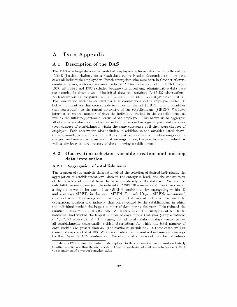
A.1 Description of the DAS

The DAS is a large data set of matched employer-employee information collected by

INSEE (Institut National de la Statistique et des Etudes Economiques). The data

cover all individuals employed in French enterprises who were born in October of even-

numbered years, with civil servants excluded.12

Our extract runs from 1976 through

1987, with 1981 and 1983 excluded because the underlying administrative data were

not sampled in those years. The initial data set contained 7,416,422 observations.

Each observation corresponds to a unique establishment-individual-year combination.

The observation includes an identi�er that corresponds to the employee (called ID

below), an identi�er that corresponds to the establishment (SIRET) and an identi�er

that corresponds to the parent enterprise of the establishment (SIREN). We have

information on the number of days the individual worked in the establishment, as

well as the full-time/part-time status of the employee. This allows us to aggregate

all of the establishments in which an individual worked in a given year, and thus not

treat changes of establishment within the same enterprise as if they were changes of

employer. Each observation also includes, in addition to the variables listed above,

the sex, month, year and place of birth, occupation, total net nominal earnings during

the year and annualized gross nominal earnings during the year for the individual, as

well as the location and industry of the employing establishment.

A.2 Observation selection variable creation and missing

data imputation

A.2.1 Aggregation of establishments

The creation of the analysis data set involved the selection of desired individuals, the

aggregation of establishment-level data to the enterprise level, and the construction

of the variables of interest from the variables already in the data set. We selected

only full-time employees (sample reduced to 5,966,620 observations). We then created

a single observation for each ID-year-SIREN combination by aggregating within ID

and year over SIRETs in the same SIREN. For each ID-year-SIREN, we summed

total net nominal earnings and total days worked over all SIRETs. We used the

occupation, location and industry that corresponded to the establishment in which

the individual worked the largest number of days during the year. This reduced the

number of observations to 5,965,256. We then selected the enterprise at which the

individual had worked the largest number of days during that year (sample reduced

to 5,497,287 observations). The aggregation of total number of days worked across

all establishments occasionally yielded observations for which the total number of

days worked was greater than 360 (the maximum permitted). In these cases, we just

truncated days worked at 360. We then calculated an annualized net nominal earnings

for the ID-year SIREN combination. We eliminated all years of data for individuals

12Meron (1988) shows that individuals employed in the civil service move almost exclusively

to other positions within the civil service. Thus the exclusion of civil servants does not a�ect

the estimation of a worker's market value.

32

who were younger than 15 years old or older than 65 years old at the date of their �rst

appearance in the data set (sample reduced to 5,325,413 observations).

A.2.2 Total compensation costs

The dependent variable in our wage rate analysis is the annualized real total com-

pensation cost of the employee (LFRAISRE). To convert the annualized net nominal

earnings to total compensation costs, we used the tax rules and computer programs

provided by the Division Revenus at INSEE (J.L. Lh�eritier, private communication)

to compute both the employee and employer share of all mandatory payroll taxes (co-

tisations et charges salariales employ�e et employeur) Total annualized compensation

cost is de�ned as the sum of annualized net nominal earnings, employee payroll taxes

and employer payroll taxes. Nominal values were then de ated by a consumer price

index to get real annualized net earnings, and real annualized total compensation cost.

We eliminated 61 observations with zero values for annualized total compensation cost

(remaining sample 5,325,352).

A.2.3 Education and Total Labor Market Experience

Our initial DAS �le did not contain education information. We used supplementary

information available for 10% of the DAS, (EDP, Echantillon D�emographique Per-

manent) to impute the level of education of all individuals in the DAS.13 The EDP

includes information on the highest degree obtained. There were 38 possible responses,

including \no known degree." These responses were grouped into 8 degree-level cat-

egories as shown in table 1. Using these eight categories and data available in the

DAS, we ran separate ordered logits for men and women to estimate coe�cients used

to impute education for the individuals in the DAS who are not part of the EDP. EDP

sample statistics for the men are in table 2, and those for the women are in table 3.

The estimated logit equations are in table 4 for men and table 5 for women.

13Access to the EDP is particularly di�cult to obtain due to privacy regulations.

33

Table 1: Degree CategoriesCategory Degree U.S. Equivalent

1 Sans Aucun Diplome No Terminal Degree

2 CEP Elementary School

DFEO

3 BEPC Junior High School

BE

BEPS

4 BAC (not F, G or H) High School

Brevet superieur

CFES

5 CAP Vocational-Technical School (Basic)

BEP

EFAA

BAA

BPA

FPA 1er

6 BP Vocational-Technical School (Advanced)

BEA

BEC

BEH

BEI

BES

BATA

BAC F

BAC G

BAC H

7 Sant�e Technical College and

BTS Undergraduate University

DUT

DEST

DEUL

DEUS

DEUG

8 2�eme cycle Graduate School and Other

3�eme cycle Post-Secondary Education

Grande �ecole

CAPES

CAPET

34

Table 2: EDP Sample Statistics - Men (Std. Deviations in Parentheses)Variable Degree Category

Name Overall 1 2 3 4 5 6 7 8

DOBi � 1924 0.188 0.254 0.295 0.160 0.136 0.055 0.098 0.063 0.186(0.391) (0.435) (0.456) (0.367) (0.343) (0.228) (0.297) (0.243) (0.389)

1925 � DOBi � 1929 0.056 0.062 0.085 0.042 0.049 0.034 0.048 0.026 0.065(0.230) (0.242) (0.279) (0.200) (0.215) (0.180) (0.214) (0.158) (0.247)

1930 � DOBi � 1934 0.097 0.109 0.120 0.067 0.068 0.081 0.095 0.054 0.101(0.296) (0.311) (0.325) (0.250) (0.252) (0.273) (0.293) (0.226) (0.301)

1935 � DOBi � 1939 0.061 0.056 0.070 0.048 0.048 0.063 0.079 0.047 0.078(0.240) (0.229) (0.255) (0.214) (0.215) (0.244) (0.270) (0.212) (0.268)

1940 � DOBi � 1944 0.094 0.070 0.091 0.075 0.098 0.117 0.133 0.118 0.149(0.292) (0.256) (0.287) (0.264) (0.298) (0.322) (0.340) (0.323) (0.356)

1945 � DOBi � 1949 0.102 0.064 0.097 0.099 0.130 0.130 0.152 0.175 0.164(0.302) (0.244) (0.296) (0.299) (0.336) (0.336) (0.359) (0.380) (0.370)

1950 � DOBi � 1954 0.159 0.095 0.132 0.166 0.245 0.224 0.217 0.288 0.201(0.365) (0.293) (0.339) (0.372) (0.430) (0.417) (0.412) (0.453) (0.401)

1955 � DOBi � 1959 0.101 0.072 0.060 0.182 0.157 0.145 0.110 0.176 0.054(0.302) (0.259) (0.238) (0.386) (0.364) (0.352) (0.313) (0.381) (0.226)

1960 � DOBi � 1976 0.141 0.218 0.050 0.160 0.069 0.151 0.068 0.052 0.003(0.348) (0.413) (0.218) (0.367) (0.253) (0.358) (0.251) (0.224) (0.056)

Works in Ile de France 0.232 0.204 0.226 0.288 0.352 0.187 0.284 0.309 0.457(0.422) (0.403) (0.418) (0.453) (0.478) (0.390) (0.451) (0.462) (0.498)

CSP62 0.263 0.357 0.282 0.188 0.157 0.199 0.145 0.184 0.105(0.440) (0.479) (0.450) (0.391) (0.364) (0.399) (0.352) (0.387) (0.307)

CSP61 0.225 0.231 0.255 0.117 0.071 0.299 0.186 0.096 0.058(0.418) (0.422) (0.436) (0.321) (0.266) (0.458) (0.390) (0.295) (0.233)

CSP50 0.151 0.118 0.166 0.279 0.279 0.108 0.203 0.235 0.203(0.358) (0.322) (0.372) (0.448) (0.448) (0.310) (0.402) (0.424) (0.402)

CSP40 0.112 0.061 0.110 0.173 0.233 0.080 0.258 0.275 0.225(0.315) (0.240) (0.314) (0.379) (0.423) (0.272) (0.438) (0.447) (0.418)

CSP30 0.043 0.020 0.025 0.053 0.147 0.015 0.057 0.080 0.359(0.203) (0.142) (0.157) (0.224) (0.354) (0.121) (0.232) (0.271) (0.480)

Number of Observations 71229 26236 12825 3847 3036 16489 3878 2387 2531

35

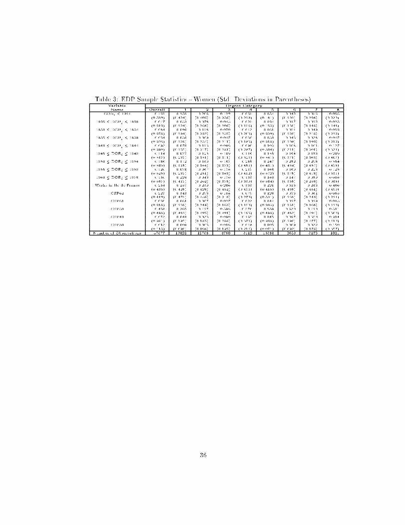
Table 3: EDP Sample Statistics - Women (Std. Deviations in Parentheses)Variable Degree Category

Name Overall 1 2 3 4 5 6 7 8

DOBi � 1924 0.152 0.235 0.206 0.129 0.055 0.034 0.042 0.055 0.056(0.359) (0.424) (0.405) (0.336) (0.229) (0.181) (0.202) (0.228) (0.230)

1925 � DOBi � 1929 0.047 0.053 0.078 0.045 0.025 0.024 0.017 0.022 0.023(0.212) (0.224) (0.268) (0.206) (0.156) (0.153) (0.130) (0.146) (0.148)

1930 � DOBi � 1934 0.084 0.096 0.118 0.070 0.043 0.061 0.054 0.049 0.052(0.278) (0.294) (0.322) (0.255) (0.203) (0.239) (0.226) (0.216) (0.222)

1935 � DOBi � 1939 0.054 0.056 0.069 0.047 0.036 0.050 0.045 0.038 0.047(0.226) (0.229) (0.254) (0.211) (0.185) (0.218) (0.208) (0.190) (0.212)

1940 � DOBi � 1944 0.093 0.070 0.113 0.086 0.090 0.103 0.108 0.101 0.127(0.290) (0.255) (0.317) (0.281) (0.287) (0.304) (0.311) (0.301) (0.334)

1945 � DOBi � 1949 0.114 0.077 0.125 0.109 0.116 0.135 0.164 0.156 0.209(0.317) (0.267) (0.331) (0.311) (0.321) (0.341) (0.371) (0.363) (0.407)

1950 � DOBi � 1954 0.186 0.112 0.180 0.167 0.285 0.247 0.252 0.298 0.354(0.389) (0.315) (0.384) (0.373) (0.451) (0.431) (0.434) (0.457) (0.478)

1955 � DOBi � 1959 0.120 0.078 0.067 0.178 0.217 0.166 0.169 0.223 0.125(0.325) (0.267) (0.251) (0.383) (0.412) (0.372) (0.375) (0.416) (0.331)

1960 � DOBi � 1976 0.150 0.224 0.043 0.170 0.133 0.180 0.147 0.059 0.008(0.357) (0.417) (0.202) (0.375) (0.339) (0.384) (0.355) (0.236) (0.088)

Works in Ile de France 0.254 0.237 0.239 0.286 0.333 0.221 0.316 0.283 0.466(0.435) (0.425) (0.426) (0.452) (0.471) (0.415) (0.465) (0.451) (0.499)

CSP62 0.227 0.343 0.296 0.108 0.079 0.126 0.073 0.061 0.053(0.419) (0.475) (0.456) (0.310) (0.270) (0.331) (0.259) (0.240) (0.224)

CSP61 0.050 0.061 0.067 0.027 0.023 0.044 0.027 0.029 0.015(0.218) (0.239) (0.249) (0.163) (0.150) (0.205) (0.161) (0.168) (0.120)

CSP50 0.458 0.365 0.427 0.596 0.570 0.539 0.630 0.420 0.511(0.498) (0.482) (0.495) (0.491) (0.495) (0.498) (0.483) (0.494) (0.500)

CSP40 0.073 0.040 0.035 0.090 0.165 0.045 0.097 0.350 0.214(0.261) (0.195) (0.185) (0.286) (0.371) (0.208) (0.296) (0.477) (0.410)

CSP30 0.013 0.008 0.005 0.016 0.048 0.005 0.009 0.032 0.150(0.115) (0.090) (0.068) (0.125) (0.214) (0.071) (0.093) (0.176) (0.357)

Number of Observations 57677 19822 12768 4760 3112 10388 2633 3173 1021

36

Table 4: Degree Category Model Coe�cients-MenDegree Variable Coe�cient Std. Err.

1 Intercept 6.254 0.122

1925 � Date of Birth � 1929 -0.496 0.105

1930 � Date of Birth � 1934 -0.493 0.090

1935 � Date of Birth � 1939 -1.234 0.100

1940 � Date of Birth � 1944 -2.031 0.085

1945 � Date of Birth � 1949 -2.818 0.085

1950 � Date of Birth � 1954 -3.388 0.086

1955 � Date of Birth � 1959 -2.289 0.113

1960 � Date of Birth � 1976 1.897 0.360

Unskilled Blue-Collar Worker at Date t in Firm J(i; t) -0.850 0.116

Skilled Blue-Collar Worker at Date t in Firm J(i; t) -0.904 0.132

Unskilled White-Collar Worker at Date t in Firm J(i; t) -2.758 0.111

Skilled White-Collar Worker at Date t in Firm J(i; t) -4.028 0.117

Manager at Date t in Firm J(i; t) -5.892 0.124

Works in Ile de France -0.627 0.048

2 Intercept 5.828 0.125

1925 � Date of Birth � 1929 -0.320 0.106

1930 � Date of Birth � 1934 -0.518 0.091

1935 � Date of Birth � 1939 -1.117 0.102

1940 � Date of Birth � 1944 -1.863 0.087

1945 � Date of Birth � 1949 -2.430 0.087

1950 � Date of Birth � 1954 -3.248 0.089

1955 � Date of Birth � 1959 -2.649 0.119

1960 � Date of Birth � 1976 0.246 0.363

Unskilled Blue-Collar Worker at Date t in Firm J(i; t) -1.311 0.119

Skilled Blue-Collar Worker at Date t in Firm J(i; t) -1.074 0.135

Unskilled White-Collar Worker at Date t in Firm J(i; t) -2.635 0.114

Skilled White-Collar Worker at Date t in Firm J(i; t) -3.740 0.121

Manager at Date t in Firm J(i; t) -5.996 0.132

Works in Ile de France -0.629 0.050

37

Degree Variable Coe�cient Std. Err.

3 Intercept 2.465 0.134

1925 � Date of Birth � 1929 -0.333 0.131

1930 � Date of Birth � 1934 -0.344 0.112

1935 � Date of Birth � 1939 -0.667 0.124

1940 � Date of Birth � 1944 -1.120 0.105

1945 � Date of Birth � 1949 -1.307 0.102

1950 � Date of Birth � 1954 -1.373 0.100

1955 � Date of Birth � 1959 0.074 0.123

1960 � Date of Birth � 1976 2.891 0.364

Unskilled Blue-Collar Worker at Date t in Firm J(i; t) -0.681 0.126

Skilled Blue-Collar Worker at Date t in Firm J(i; t) -0.557 0.144

Unskilled White-Collar Worker at Date t in Firm J(i; t) -0.944 0.118

Skilled White-Collar Worker at Date t in Firm J(i; t) -1.610 0.127

Manager at Date t in Firm J(i; t) -3.400 0.142

Works in Ile de France -0.410 0.057

4 Intercept 0.803 0.142

1925 � Date of Birth � 1929 0.005 0.133

1930 � Date of Birth � 1934 -0.109 0.117

1935 � Date of Birth � 1939 -0.325 0.130

1940 � Date of Birth � 1944 -0.381 0.106

1945 � Date of Birth � 1949 -0.379 0.104

1950 � Date of Birth � 1954 -0.069 0.101

1955 � Date of Birth � 1959 0.830 0.127

1960 � Date of Birth � 1976 2.855 0.369

Unskilled Blue-Collar Worker at Date t in Firm J(i; t) -0.193 0.134

Skilled Blue-Collar Worker at Date t in Firm J(i; t) -0.294 0.156

Unskilled White-Collar Worker at Date t in Firm J(i; t) -0.217 0.125

Skilled White-Collar Worker at Date t in Firm J(i; t) -0.377 0.132

Manager at Date t in Firm J(i; t) -1.311 0.136

Works in Ile de France -0.265 0.057

38

Degree Variable Coe�cient Std. Err.

5 Intercept 3.985 0.125

1925 � Date of Birth � 1929 0.392 0.113

1930 � Date of Birth � 1934 0.734 0.096

1935 � Date of Birth � 1939 0.446 0.105

1940 � Date of Birth � 1944 0.090 0.089

1945 � Date of Birth � 1949 -0.336 0.089

1950 � Date of Birth � 1954 0.700 0.090

1955 � Date of Birth � 1959 0.230 0.116

1960 � Date of Birth � 1976 3.319 0.362

Unskilled Blue-Collar Worker at Date t in Firm J(i; t) -1.306 0.116

Skilled Blue-Collar Worker at Date t in Firm J(i; t) -0.340 0.131

Unskilled White-Collar Worker at Date t in Firm J(i; t) -2.494 0.110

Skilled White-Collar Worker at Date t in Firm J(i; t) -3.011 0.117

Manager at Date t in Firm J(i; t) -5.195 0.131

Works in Ile de France -0.766 0.049

6 Intercept 1.714 0.139

1925 � Date of Birth � 1929 0.266 0.132

1930 � Date of Birth � 1934 0.471 0.111

1935 � Date of Birth � 1939 0.318 0.119

1940 � Date of Birth � 1944 0.000 0.102

1945 � Date of Birth � 1949 -0.216 0.102

1950 � Date of Birth � 1954 -0.363 0.103

1955 � Date of Birth � 1959 0.312 0.130

1960 � Date of Birth � 1976 2.742 0.368

Unskilled Blue-Collar Worker at Date t in Firm J(i; t) -0.849 0.129

Skilled Blue-Collar Worker at Date t in Firm J(i; t) -0.006 0.142

Unskilled White-Collar Worker at Date t in Firm J(i; t) -1.100 0.121

Skilled White-Collar Worker at Date t in Firm J(i; t) -1.030 0.126

Manager at Date t in Firm J(i; t) -3.036 0.141

Works in Ile de France -0.510 0.056

39

Degree Variable Coe�cient Std. Err.

7 Intercept -0.141 0.158

1925 � Date of Birth � 1929 0.102 0.179

1930 � Date of Birth � 1934 0.407 0.145

1935 � Date of Birth � 1939 0.349 0.154

1940 � Date of Birth � 1944 0.519 0.126

1945 � Date of Birth � 1949 0.653 0.123

1950 � Date of Birth � 1954 0.843 0.121

1955 � Date of Birth � 1959 1.704 0.145

1960 � Date of Birth � 1976 3.339 0.379

Unskilled Blue-Collar Worker at Date t in Firm J(i; t) -0.155 0.136

Skilled Blue-Collar Worker at Date t in Firm J(i; t) -0.055 0.157

Unskilled White-Collar Worker at Date t in Firm J(i; t) -0.437 0.129

Skilled White-Collar Worker at Date t in Firm J(i; t) -0.100 0.134

Manager at Date t in Firm J(i; t) -1.648 0.148

Works in Ile de France -0.399 0.062

40

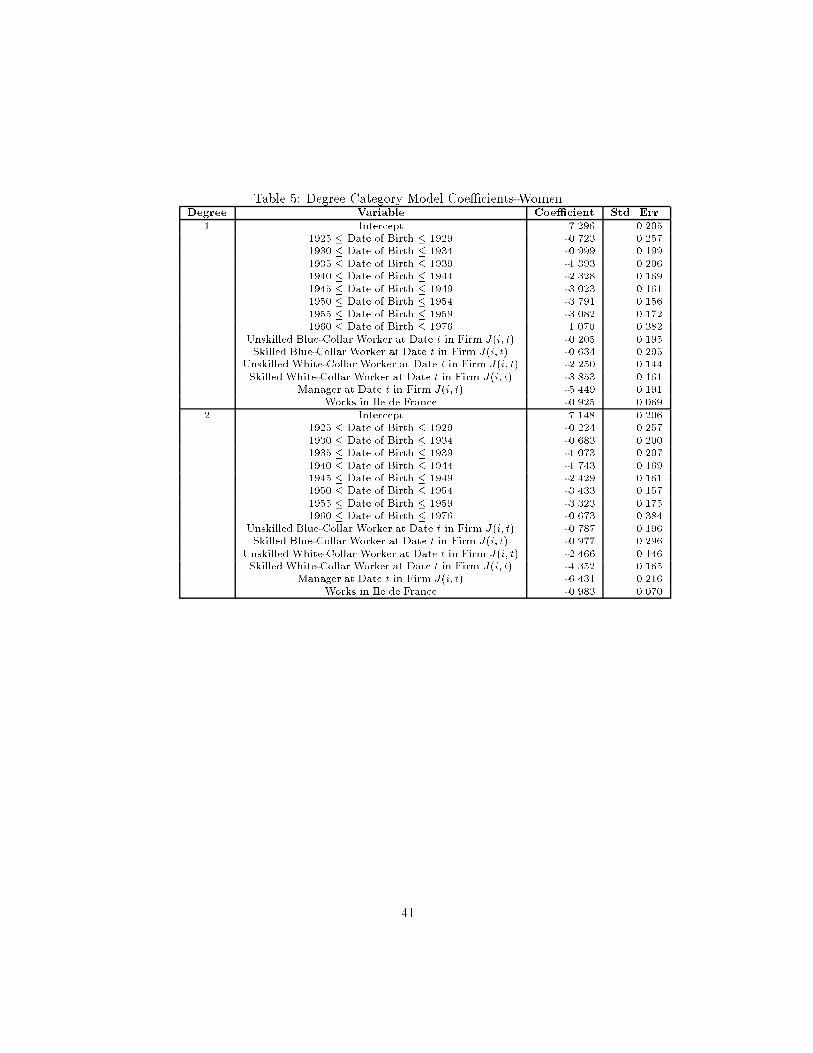
Table 5: Degree Category Model Coe�cients-WomenDegree Variable Coe�cient Std. Err.

1 Intercept 7.296 0.205

1925 � Date of Birth � 1929 -0.723 0.257

1930 � Date of Birth � 1934 -0.999 0.199

1935 � Date of Birth � 1939 -1.393 0.206

1940 � Date of Birth � 1944 -2.328 0.169

1945 � Date of Birth � 1949 -3.023 0.161

1950 � Date of Birth � 1954 -3.791 0.156

1955 � Date of Birth � 1959 -3.082 0.172

1960 � Date of Birth � 1976 1.070 0.382

Unskilled Blue-Collar Worker at Date t in Firm J(i; t) -0.205 0.195

Skilled Blue-Collar Worker at Date t in Firm J(i; t) -0.634 0.295

Unskilled White-Collar Worker at Date t in Firm J(i; t) -2.250 0.144

Skilled White-Collar Worker at Date t in Firm J(i; t) -3.853 0.161

Manager at Date t in Firm J(i; t) -5.449 0.191

Works in Ile de France -0.925 0.069

2 Intercept 7.148 0.206

1925 � Date of Birth � 1929 -0.224 0.257

1930 � Date of Birth � 1934 -0.683 0.200

1935 � Date of Birth � 1939 -1.073 0.207

1940 � Date of Birth � 1944 -1.743 0.169

1945 � Date of Birth � 1949 -2.429 0.161

1950 � Date of Birth � 1954 -3.433 0.157

1955 � Date of Birth � 1959 -3.323 0.175

1960 � Date of Birth � 1976 -0.673 0.384

Unskilled Blue-Collar Worker at Date t in Firm J(i; t) -0.787 0.196

Skilled Blue-Collar Worker at Date t in Firm J(i; t) -0.977 0.296

Unskilled White-Collar Worker at Date t in Firm J(i; t) -2.466 0.146

Skilled White-Collar Worker at Date t in Firm J(i; t) -4.352 0.165

Manager at Date t in Firm J(i; t) -6.431 0.216

Works in Ile de France -0.983 0.070

41

Degree Variable Coe�cient Std. Err.

3 Intercept 4.645 0.211

1925 � Date of Birth � 1929 -0.307 0.265

1930 � Date of Birth � 1934 -0.742 0.207

1935 � Date of Birth � 1939 -1.021 0.217

1940 � Date of Birth � 1944 -1.550 0.177

1945 � Date of Birth � 1949 -2.011 0.167

1950 � Date of Birth � 1954 -2.537 0.162

1955 � Date of Birth � 1959 -1.409 0.176

1960 � Date of Birth � 1976 1.506 0.385

Unskilled Blue-Collar Worker at Date t in Firm J(i; t) -0.778 0.202

Skilled Blue-Collar Worker at Date t in Firm J(i; t) -0.840 0.308

Unskilled White-Collar Worker at Date t in Firm J(i; t) -1.218 0.149

Skilled White-Collar Worker at Date t in Firm J(i; t) -2.379 0.166

Manager at Date t in Firm J(i; t) -3.977 0.209

Works in Ile de France -0.738 0.074

4 Intercept 2.263 0.223

1925 � Date of Birth � 1929 0.023 0.285

1930 � Date of Birth � 1934 -0.314 0.225

1935 � Date of Birth � 1939 -0.383 0.233

1940 � Date of Birth � 1944 -0.542 0.189

1945 � Date of Birth � 1949 -0.894 0.180

1950 � Date of Birth � 1954 -0.694 0.172

1955 � Date of Birth � 1959 0.075 0.187

1960 � Date of Birth � 1976 2.448 0.390

Unskilled Blue-Collar Worker at Date t in Firm J(i; t) -0.248 0.210

Skilled Blue-Collar Worker at Date t in Firm J(i; t) -0.167 0.320

Unskilled White-Collar Worker at Date t in Firm J(i; t) -0.502 0.154

Skilled White-Collar Worker at Date t in Firm J(i; t) -0.880 0.169

Manager at Date t in Firm J(i; t) -1.725 0.193

Works in Ile de France -0.462 0.076

42

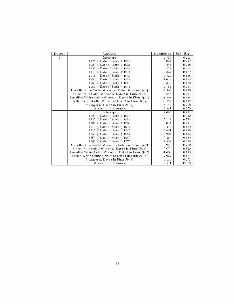
Degree Variable Coe�cient Std. Err.

5 Intercept 4.555 0.211

1925 � Date of Birth � 1929 0.391 0.267

1930 � Date of Birth � 1934 0.441 0.208

1935 � Date of Birth � 1939 0.371 0.214

1940 � Date of Birth � 1944 -0.057 0.177

1945 � Date of Birth � 1949 -0.529 0.168

1950 � Date of Birth � 1954 -1.022 0.163

1955 � Date of Birth � 1959 -0.342 0.178

1960 � Date of Birth � 1976 2.753 0.385

Unskilled Blue-Collar Worker at Date t in Firm J(i; t) -0.898 0.196

Skilled Blue-Collar Worker at Date t in Firm J(i; t) -0.645 0.297

Unskilled White-Collar Worker at Date t in Firm J(i; t) -1.593 0.144

Skilled White-Collar Worker at Date t in Firm J(i; t) -3.272 0.162

Manager at Date t in Firm J(i; t) -5.147 0.218

Works in Ile de France -0.967 0.070

6 Intercept 2.693 0.231

1925 � Date of Birth � 1929 -0.148 0.309

1930 � Date of Birth � 1934 0.111 0.233

1935 � Date of Birth � 1939 0.054 0.241

1940 � Date of Birth � 1944 -0.210 0.199

1945 � Date of Birth � 1949 -0.461 0.189

1950 � Date of Birth � 1954 -0.927 0.184

1955 � Date of Birth � 1959 -0.264 0.199

1960 � Date of Birth � 1976 2.531 0.396

Unskilled Blue-Collar Worker at Date t in Firm J(i; t) -0.969 0.212

Skilled Blue-Collar Worker at Date t in Firm J(i; t) -0.675 0.320

Unskilled White-Collar Worker at Date t in Firm J(i; t) -1.008 0.153

Skilled White-Collar Worker at Date t in Firm J(i; t) -2.062 0.174

Manager at Date t in Firm J(i; t) -4.133 0.272

Works in Ile de France -0.541 0.078

43

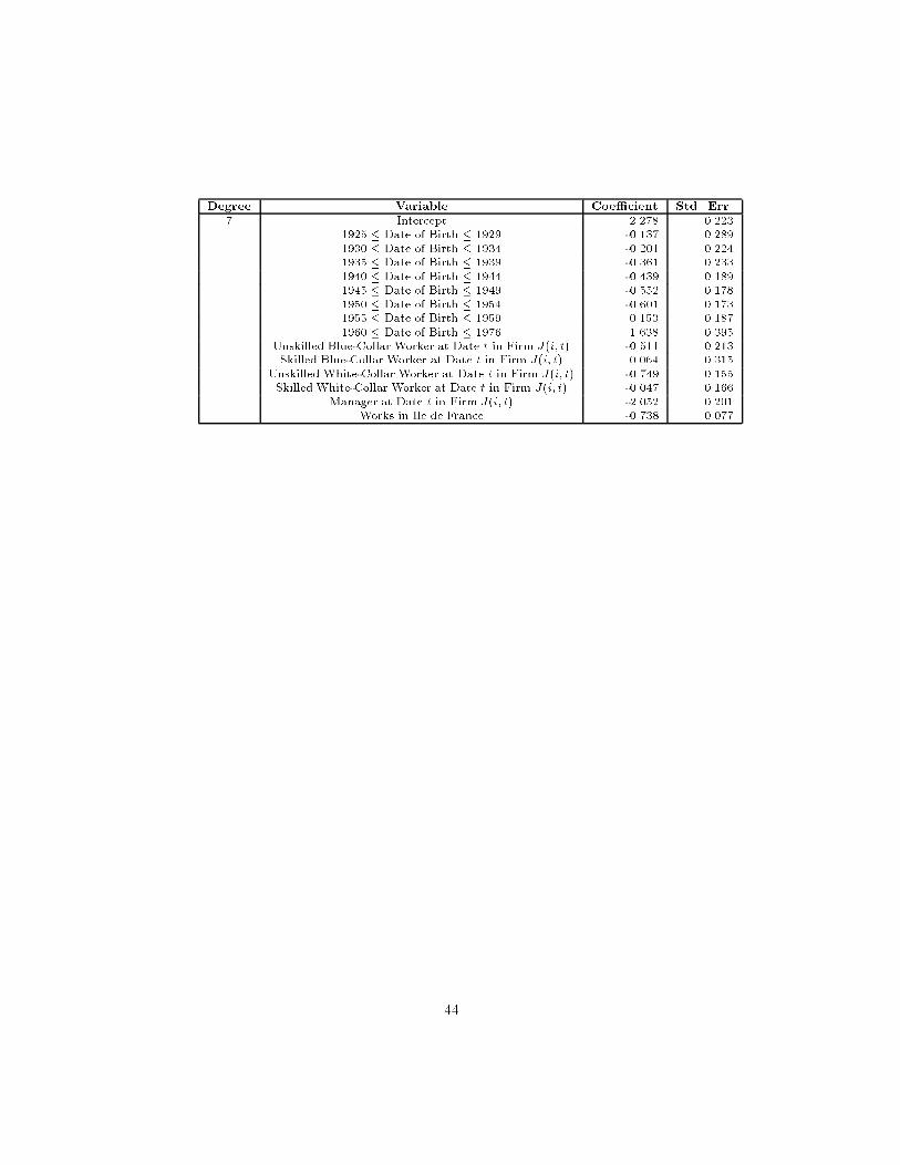
Degree Variable Coe�cient Std. Err.

7 Intercept 2.278 0.223

1925 � Date of Birth � 1929 -0.137 0.289

1930 � Date of Birth � 1934 -0.201 0.224

1935 � Date of Birth � 1939 -0.361 0.233

1940 � Date of Birth � 1944 -0.439 0.189

1945 � Date of Birth � 1949 -0.552 0.178

1950 � Date of Birth � 1954 -0.601 0.173

1955 � Date of Birth � 1959 0.153 0.187

1960 � Date of Birth � 1976 1.638 0.395

Unskilled Blue-Collar Worker at Date t in Firm J(i; t) -0.511 0.213

Skilled Blue-Collar Worker at Date t in Firm J(i; t) 0.064 0.315

Unskilled White-Collar Worker at Date t in Firm J(i; t) -0.749 0.155

Skilled White-Collar Worker at Date t in Firm J(i; t) -0.047 0.166

Manager at Date t in Firm J(i; t) -2.052 0.201

Works in Ile de France -0.738 0.077

44

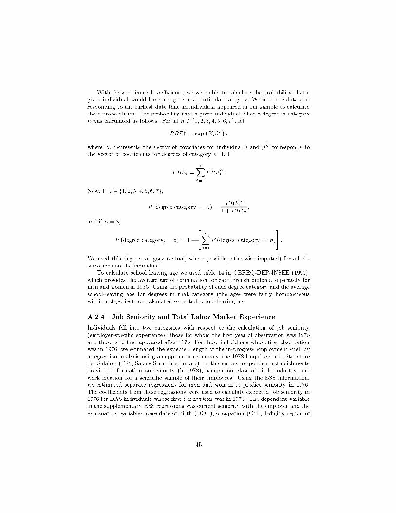
With these estimated coe�cients, we were able to calculate the probability that a

given individual would have a degree in a particular category. We used the data cor-

responding to the earliest date that an individual appeared in our sample to calculate

these probabilities. The probability that a given individual i has a degree in category

n was calculated as follows. For all ~n 2 f1; 2; 3; 4; 5; 6; 7g, let

PRE~ni = exp

�Xi�

~n�;

where Xi represents the vector of covariates for individual i and �~n corresponds to

the vector of coe�cients for degrees of category ~n. Let

PREi =

7X~n=1

PRE~ni :

Now, if n 2 f1; 2; 3; 4; 5; 6; 7g,

P (degree categoryi = n) =PREn

i

1 + PREi

;

and if n = 8,

P (degree categoryi = 8) = 1�

"7X

~n=1

P (degree categoryi = ~n)

#:

We used this degree category (actual, where possible, otherwise imputed) for all ob-

servations on the individual.

To calculate school leaving age we used table 14 in CEREQ-DEP-INSEE (1990),

which provides the average age of termination for each French diploma separately for

men and women in 1986. Using the probability of each degree category and the average

school-leaving age for degrees in that category (the ages were fairly homogeneous

within categories), we calculated expected school-leaving age.

A.2.4 Job Seniority and Total Labor Market Experience

Individuals fell into two categories with respect to the calculation of job seniority

(employer-speci�c experience): those for whom the �rst year of observation was 1976

and those who �rst appeared after 1976. For those individuals whose �rst observation

was in 1976, we estimated the expected length of the in-progress employment spell by

a regression analysis using a supplementary survey, the 1978 Enquete sur la Structure

des Salaires (ESS, Salary Structure Survey). In this survey, respondent establishments

provided information on seniority (in 1978), occupation, date of birth, industry, and

work location for a scienti�c sample of their employees. Using the ESS information,

we estimated separate regressions for men and women to predict seniority in 1976.

The coe�cients from these regressions were used to calculate expected job seniority in

1976 for DAS individuals whose �rst observation was in 1976. The dependent variable

in the supplementary ESS regressions was current seniority with the employer and the

explanatory variables were date of birth (DOB), occupation (CSP, 1-digit), region of

45

employment (metropolitan Paris), and industry (NAP 100, approximately 2-digit).14

Table 6 provides sample statistics for the ESS data. Results of these regressions are

Table 6: ESS Variables and Means (Std. Deviations in Parentheses)Variable Mean-Men Mean-Women

Seniorityi;t;J(i;t) 10.244 7.910

(9.271) (7.796)

DOBi � 1924 0.113 0.095

(0.317) (0.293)

1925 � DOBi � 1929 0.112 0.087

(0.315) (0.281)

1930 � DOBi � 1934 0.124 0.097

(0.330) (0.296)

1935 � DOBi � 1939 0.115 0.088

(0.319) (0.283)

1940 � DOBi � 1944 0.111 0.087

(0.314) (0.282)

1945 � DOBi � 1949 0.153 0.145

(0.360) (0.352)

1950 � DOBi � 1954 0.154 0.188

(0.361) (0.391)

1955 � DOBi � 1959 0.094 0.174

(0.292) (0.379)

Worked in Ile de Francei;t;J(i;t) 0.191 0.233

(0.393) (0.423)

CSP30i;t;J(i;t) 0.106 0.026

(0.308) (0.161)

CSP40i;t;J(i;t) 0.175 0.072

(0.380) (0.258)

CSP50i;t;J(i;t) 0.180 0.492

(0.384) (0.500)

CSP61i;t;J(i;t) 0.283 0.064

(0.450) (0.245)

CSP62i;t;J(i;t) 0.256 0.346

(0.437) (0.476)

14The excluded categories were: 1960�DOBi, CSP62 (1 if i is an Unskilled Blue-Collar

Worker at Date t in �rm J(i; t)), and N89 (1 if �rm J(i; t) is in industry 89, Financial Orga-

nizations). The coe�cients on the industry indicators are not shown below.

46

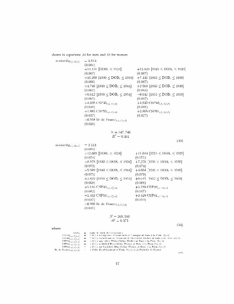
shown in equations 33 for men and 34 for women.

seniorityi;t;J(i;t) = 2:513

(0:081)

+14:151 [DOBi � 1924] +12:820 [1925 � DOBi � 1929]

(0:067) (0:067)

+10:299 [1930 � DOBi � 1934] +7:445 [1935 � DOBi � 1939]

(0:066) (0:067)

+4:748 [1940 � DOBi � 1944] +2:569 [1945 � DOBi � 1949]

(0:067) (0:065)

+0:612 [1950 � DOBi � 1954] �0:642 [1955 � DOBi � 1959]

(0:065) (0:067)

+4:039 CSP30i;t;J(i;t) +4:939 CSP40i;t;J(i;t)(0:038) (0:031)

+1:885 CSP50i;t;J(i;t) +2:898 CSP61i;t;J(i;t)(0:037) (0:027)

�0:958 Ile de Francei;t;J(i;t)(0:026)

N = 547; 746

R2 = 0:461

(33)

seniorityi;t;J(i;t) = 2:114

(0:084)

+12:669 [DOBi � 1924] +11:014 [1925 � DOBi � 1929]

(0:074) (0:075)

+8:979 [1930 � DOBi � 1934] +7:278 [1935 � DOBi � 1939]

(0:073) (0:074)

+5:989 [1940 � DOBi � 1944] +4:604 [1945 � DOBi � 1949]

(0:075) (0:070)

+2:822 [1950 � DOBi � 1954] +0:641 [1955 � DOBi � 1959]

(0:068) (0:068)

+5:116 CSP30i;t;J(i;t) +5:789 CSP40i;t;J(i;t)(0:082) (0:057)

+1:442 CSP50i;t;J(i;t) +2:429 CSP61i;t;J(i;t)(0:037) (0:054)

�0:988 Ile de Francei;t;J(i;t)(0:031)

N = 260; 580

R2 = 0:373

(34)

where

DOBi = Date of Birth of Individual iCSP30i;t;J(i;t) = 1 if i is a Engineer, Professional or Manager at Date t in Firm J(i; t)

CSP40i;t;J(i;t) = 1 if i is Technician or Technical White-Collar Worker at Date t in Firm J(i; t)

CSP50i;t;J(i;t) = 1 if i is any other White-Collar Worker at Date t in Firm J(i; t)

CSP61i;t;J(i;t) = 1 if i is a Skilled Blue-Collar Worker at Date t in Firm J(i; t)

CSP62i;t;J(i;t) = 1 if i is an Unskilled Blue-Collar Worker at Date t in Firm J(i; t)

Ile de Francei;t;J(i;t) = 1 if the Establishment of Firm J(i; t) is in Paris-Ile de France.

(35)

47

We used these results to impute levels of job seniority in 1976 for the left-censored DAS individuals �rst observed in 1976. If the individual was left-censored and the imputed job seniority was negative, we set job seniority priorto 1976 to zero. If the individual was �rst observed after 1976, we assumed thatjob seniority prior to the date of the �rst DAS observation for the individual waszero. If the age at the date of any observation (1976 or otherwise) was less thanthe expected school-leaving age, both total labor force experience and prior jobseniority were set to zero. In all other cases (when the age was greater thanthe expected school-leaving age), we calculated total labor market experienceand job seniority as follows. If the observation was the earliest appearanceof the individual in our data, we set job seniority equal to job seniority upto the date of the �rst observation plus the number of days worked for thatenterprise in the year of the �rst observation, divided by 360 and we set totallabor market experience to the current age less the school-leaving age. If theobservation was not the �rst for the individual but there was an observation inthe previous year for the person15, we added 1 to total labor market experience.If the individual was employed for the majority of the current year by thesame enterprise that employed him or her for the majority of the previous year,i.e. SIRENt = SIRENt�1, we added 1 to the level of seniority at t � 1. IfSIRENt 6= SIRENt�1, we set seniority equal to the number of days workeddivided by 360.

If, on the other hand, there was no observation in the previous year, wedistinguished between t =1982 or t =1984 and other years. When t 6=1982 or1984, total labor market experience was increased by 1 (re ecting experiencegained in the year of the observation). If the current SIREN and the mostrecent previous SIREN were the same, we added the number of days workedover 360 to the most previous level of seniority. This is similar to assuming thatthe worker was temporarily laid o�, but retained his or her seniority in the �rmwhen recalled. Otherwise, we set seniority to the number of days worked over360.

In the case where t =1982 or t =1984, if the preceding observation was 2years earlier (i.e. the missing data only occurred over a period when no data wereavailable for any individual), we increased total labor market experience by 2. IfSIRENt�2 = SIRENt,seniority was increased by 2. If SIRENt�2 6= SIRENt,seniority was increased by 0.5 plus the number of days worked over 36016.

15The structure of our database is such that this condition (observations for individual i

at both t and t � 1) could only fail to be satis�ed under 3 conditions. The �rst is that the

individual was employed in the civil service in the intervening years. The second is that the

individual was unemployed for an entire calendar year. The third is that t =1982 or t =1984,

since we were not given access to the data for these years. We largely discount the �rst

possibility, since full-time civil servants rarely move out of the civil service one they have

entered (Meron (1988)). The other two possibilities are treated explicitly.16We assumed that the probability the individual was reemployed in the missing year was

equal to the probability that the individual was reemployed in the observation year. Thus the

expected increment to job seniority is the share of the year worked in the observation year

48

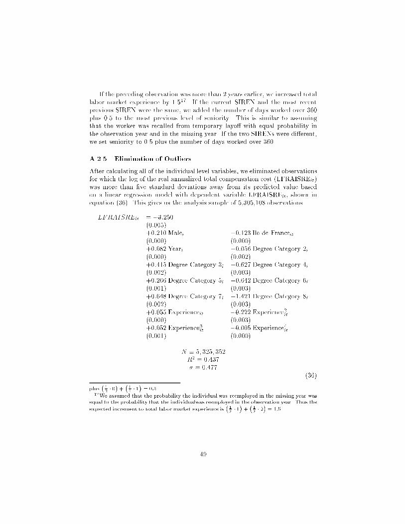
If the preceding observation was more than 2 years earlier, we increased totallabor market experience by 1.517. If the current SIREN and the most recentprevious SIREN were the same, we added the number of days worked over 360plus 0.5 to the most previous level of seniority. This is similar to assumingthat the worker was recalled from temporary layo� with equal probability inthe observation year and in the missing year. If the two SIRENs were di�erent,we set seniority to 0.5 plus the number of days worked over 360.

A.2.5 Elimination of Outliers

After calculating all of the individual level variables, we eliminated observationsfor which the log of the real annualized total compensation cost (LFRAISREit)was more than �ve standard deviations away from its predicted value basedon a linear regression model with dependent variable LFRAISREit, shown inequation (36). This gives us the analysis sample of 5,305,108 observations.

LFRAISREit = �3:250(0:005)+0:210 Malei +0:123 Ile de Franceit(0:000) (0:000)+0:082 Yeart +0:056 Degree Category 2i(0:000) (0:002)+0:415 Degree Category 3i +0:627 Degree Category 4i(0:002) (0:003)+0:266 Degree Category 5i +0:642 Degree Category 6i(0:001) (0:003)+0:648 Degree Category 7i +1:421 Degree Category 8i(0:002) (0:003)+0:055 Experienceit �0:222 Experience2it(0:000) (0:003)+0:052 Experience3it �0:005 Experience4it(0:001) (0:000)

N = 5; 325; 352R2 = 0:437� = 0:477

(36)

plus�12� 0�+�12� 1�= 0:5.

17We assumed that the probability the individual was reemployed in the missing year was

equal to the probability that the individualwas reemployed in the observation year. Thus the

expected increment to total labor market experience is�12� 1�+�12� 2�= 1:5.

49

A.3 Supplementary information on projection method vari-

ables

The derivation of the individual and �rm e�ects took place in three basic steps:an estimation of the \�rst-step equation" derived as equation (6), an extraction

and decomposition of the individual e�ect��i

�into observable (ui�) and un-

observable (�i) components, and a decomposition of the correlated component(~zit�) into the enterprise-speci�c constant e�ect (�j), the enterprise-speci�c co-e�cient on seniority ( 1j) and the enterprise-speci�c coe�cient on the linearspline at seniority of 10 years ( 2j).

A.3.1 The First-Step Regression

Equation (5) represents the projection of the �rm-speci�c variables onto �rmand individual data. In order to estimate the �rst-step equation (9), we require(in addition to the seniority variable derived in section A.2.4 above) some �rmspeci�c variable (denoted fJ(i;t)t in equation (5) and a vector of means of someindividual speci�c variables (denoted �xi in equation (5). We calculated �rm em-ployment directly from the �rms represented in the DAS data. The samplingscheme of the DAS ensures that we have a 1

25sample of the private French work-

ing population. Since we have 10 years worth of data on the French economy,we calculated fJ(i;t)as:

fJ(i;t) =(2:5�Number of DAS Observations for Firm J(i; t))

1000� 8:3:

Although this measure does not vary over time for a particular �rm, it doesvary over time for an individual who changes employers, which is the essenceof our identi�cation of �rm e�ects relative to individual e�ects. The vector xitin equation (5) includes time-varying individual-speci�c variables. The vector�xi in equation (5) contains the individual speci�c means of the two individual-speci�c variables onto which the �rm e�ect was projected: individual i's totallabor market experience and total labor market experience squared at date t.These individual-speci�c means were used in the calculation of the matrix zit.Table 7 presents the variables appearing in the matrix zit.

The �rst step equation (9) requires that the variables all be restated interms of deviations from individual-speci�c means shown below for men with

50

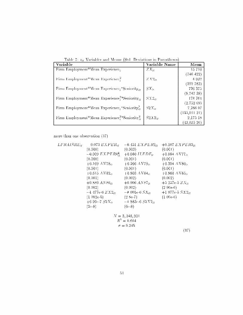
Table 7: zit Variables and Means (Std. Deviations in Parentheses)Variable Variable Name Mean

Firm Employment*Mean Experiencei ZXit 15.710(746.422)

Firm Employment*Mean Experience2i ZX2it 4.032(222.783)

Firm Employment*Mean Experiencei*Seniorityit SXit 726.375(8,747.38)

Firm Employment*Mean Experience2i*Seniorityit SX2it 178.764(2,752.69)

Firm Employment*Mean Experiencei*Seniority2it S2Xit 7,766.07

(135,011.21)Firm Employment*Mean Experience2i*Seniority

2it S2X2it 2,175.18

(43,035.26)

more than one observation (37)

LFRAISREit = 0:073 EXPERit �0:451 EXPER2it +0:107 EXPER3it(0:000) (0:003) (0:001)�0:009 EXPER44it +0:080 ILEDFit +0:084 AN77it(0:000) (0:001) (0:001)+0:169 AN78it +0:266 AN79it +0:394 AN80it(0:001) (0:001) (0:001)+0:615 AN82it +0:803 AN84it +0:860 AN85it(0:001) (0:002) (0:002)+0:880 AN86it +0:906 AN87it +5.237e-5 ZXit

(0:002) (0:002) (2.96e-6)�1.477e-6 ZX2it �8.001e-6 SXit +1.977e-5 SX2it(1.002e-5) (2.8e-7) (1.00e-6)+6.99e-7 S2Xit �1.883e-6 S2X2it(2e-8) (6e-8)

N = 3; 248; 901R2 = 0:604� = 0:245

(37)

51

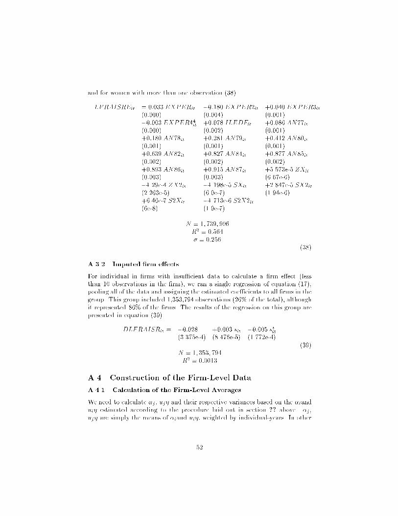
and for women with more than one observation (38).

LFRAISREit = 0:033 EXPERit �0:180 EXPER2it +0:040 EXPER3it(0:000) (0:004) (0:001)�0:003 EXPER44it +0:078 ILEDFit +0:086 AN77it(0:000) (0:002) (0:001)+0:180 AN78it +0:281 AN79it +0:412 AN80it(0:001) (0:001) (0:001)+0:639 AN82it +0:827 AN84it +0:877 AN85it(0:002) (0:002) (0:002)+0:893 AN86it +0:915 AN87it +5.573e-5 ZXit

(0:003) (0:003) (6.67e-6)�1.29e-4 ZX2it �1.198e-5 SXit +2.847e-5 SX2it(2.263e-5) (6.0e-7) (1.94e-6)+6.46e-7 S2Xit �1.713e-6 S2X2it(6e-8) (1.9e-7)

N = 1; 739; 996R2 = 0:564� = 0:256

(38)

A.3.2 Imputed �rm e�ects

For individual in �rms with insu�cient data to calculate a �rm e�ect (lessthan 10 observations in the �rm), we ran a single regression of equation (17),pooling all of the data and assigning the estimated coe�cients to all �rms in thegroup. This group included 1,353,794 observations (26% of the total), althoughit represented 86% of the �rms. The results of the regression on this group arepresented in equation (39).

DLFRAISRit = �0:028 +0:003 sit �0:005 s?it(3.375e-4) (8.476e-5) (1.772e-4)

N = 1; 353; 794R2 = 0:0013

(39)

A.4 Construction of the Firm-Level Data

A.4.1 Calculation of the Firm-Level Averages

We need to calculate �j, uj� and their respective variances based on the �iandui� estimated according to the procedure laid out in section ?? above. �j,uj� are simply the means of �iand ui�, weighted by individual-years. In other

52

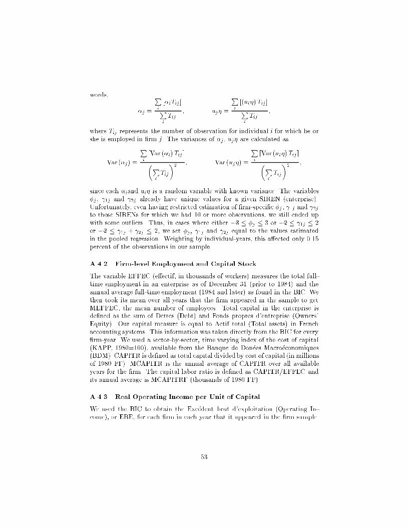
words,

�j =

Pi

[�iTij]Pi

Tij; uj� =

Pi

[(ui�)Tij]Pi

Tij;

where Tij represents the number of observation for individual i for which he orshe is employed in �rm j. The variances of �j, uj� are calculated as

Var (�j) =

Pi

[Var (�i)Tij ]�Pi

Tij

�2; Var (uj�) =

Pi

[Var (ui�)Tij ]�Pi

Tij

�2;

since each �iand ui� is a random variable with known variance. The variables�j, 1j and 2j already have unique values for a given SIREN (enterprise).Unfortunately, even having restricted estimation of �rm-speci�c �j , 1j and 2jto those SIRENs for which we had 10 or more observations, we still ended upwith some outliers. Thus, in cases where either �3 � �j � 3 or �2 � 1j � 2or �2 � 1j + 2j � 2, we set �j, 1j and 2j equal to the values estimatedin the pooled regression. Weighting by individual-years, this a�ected only 0.15percent of the observations in our sample.

A.4.2 Firm-level Employment and Capital Stock

The variable EFFEC (e�ectif, in thousands of workers) measures the total full-time employment in an enterprise as of December 31 (prior to 1984) and theannual average full-time employment (1984 and later) as found in the BIC. Wethen took its mean over all years that the �rm appeared in the sample to getMEFFEC, the mean number of employees. Total capital in the enterprise isde�ned as the sum of Dettes (Debt) and Fonds propres d'entreprise (Owners'Equity). Our capital measure is equal to Actif total (Total assets) in Frenchaccounting systems. This information was taken directly from the BIC for every�rm-year. We used a sector-by-sector, time varying index of the cost of capital(KAPP, 1980=100), available from the Banque de Don�ees Macro�economiques(BDM). CAPITR is de�ned as total capital divided by cost of capital (in millionsof 1980 FF). MCAPITR is the annual average of CAPITR over all availableyears for the �rm. The capital labor ratio is de�ned as CAPITR/EFFEC andits annual average is MCAPITRF (thousands of 1980 FF)

A.4.3 Real Operating Income per Unit of Capital

We used the BIC to obtain the Exc�edent brut d'exploitation (Operating In-come), or EBE, for each �rm in each year that it appeared in the �rm sample.

53

The formula used to calculate the EBE is shown in equation 40.

EBE = ventes de marchandises (merchandise sold)� achat de marchandises (merchandise purchased)� variation de stock de marchandises

(variation in merchandise inventory)+ ventes de biens (goods sold)+ ventes de services (services sold)+ production stock�ee (inventoried production)+ production immobilis�ee (un�nished production)� achats de mati�eres premi�eres (primary materials purchased)� variation de stocks sur mati�eres premi�eres

(variation of primary materials inventories)� autres achats et charges externes

(other purchases and outside charges)+ subventions d'exploitation (incentives for production)� impots, taxes et versements assimil�es

(value added tax and other accrued taxes onor credits for production)

� salaires et traitements (salaries and bene�ts)� charges sociales (payroll taxes)

(40)The EBE was de ated by the prix de valeur ajout�ee (value added price index),also found in the BDM, to yield EBER (thousands of 1980 FF). EBER wasdivided by CAPITR (times 1,000) to yield EBERC, real operating income perunit of capital (1980 FF). Lastly, we took the mean of EBERC over all of the�rm-years to get MEBERC, mean real operating income per unit of capital(1980 FF).

A.4.4 Real Value Added Inclusive of Labor Costs

To calculate the valeur ajout�ee r�eelle brute au cout des facteurs-(real value addedinclusive of labor costs), VABCFR, we divided the frais de personnel (employer'scompensation cost) from the BIC (thousands of FF) by the indice des prix �a laconsommation (consumer price index) from the BDM to yield the employer's realcompensation cost (thousands of 1980 FF). The results was added to EBER, asde�ned above in section A.4.3, to yield the VABCFR, real value added inclusiveof labor costs (thousands of 1980 FF). VABCFR was divided by EFFEC to yieldVABCFRF, real value added inclusive of factor costs per worker (1980 FF). Wetook the mean of VABCFRF over all of the years that the �rm appeared in thesample to get MVABCFRF, mean real value added inclusive of labor costs perworker (1980 FF).

54

A.4.5 Employment structure

The variable MING, proportion of engineers, technicians and managers in thework force (EFFEC), was calculated from the ESE using the PCS occupationclassi�cation (35) for individuals in categories 30 and 40. MOQA, the proportionof skilled workers in the work force, was calculated from the ESE using thePCS occupation classi�cation (35) for individuals in categories 50 and 61. Bothvariables were expressed as a ratio to EFFEC and averaged over all the available�rm-years.

B Model Appendix

Tables B1 to B3 show the �rst- and second-period wage equations for each of therepresentative individuals as a function of the statistical parameters of equation(1) and the parameters speci�ed in each of the theoretical models in section 3.1.

55

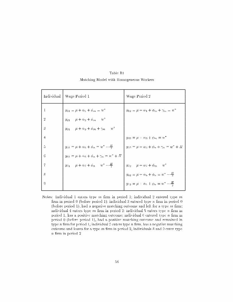
Table B1

Matching Model with Homogeneous Workers

Individual Wage Period 1 Wage Period 2

1 y11 = �+ �1 + �m = w� y12 = �+ �1 + �m + m = w�

2 y21 = �+ �2 + �m = w�

3 y31 = �+ �3 + �m + m = w�

4 y42 = �+ �3 + �m = w�

5 y51 = �+ �5 + �n = w� � H2

y52 = �+ �5 + �n + n = w� +H

6 y61 = �+ �6 + �n + n = w� +H

7 y71 = �+ �7 + �n = w� � H2

y72 = �+ �7 + �m = w�

8 y82 = �+ �8 + �n = w� � H2

9 y92 = �+ �9 + �n = w� � H2

Notes: Individual 1 enters type m �rm in period 1; individual 2 entered type m

�rm in period 0 (before period 1); individual 3 entered type n �rm in period 0(before period 1), had a negative matching outcome and left for a type m �rm;individual 4 enters type m �rm in period 2; individual 5 enters type n �rm inperiod 1, has a positive matching outcome; individual 6 entered type n �rm inperiod 0 (before period 1), had a positive matching outcome and remained intype n �rm for period 1; individual 7 enters type n �rm, has a negative matchingoutcome and leaves for a type m �rm in period 2; individuals 8 and 9 enter typen �rm in period 2.

56

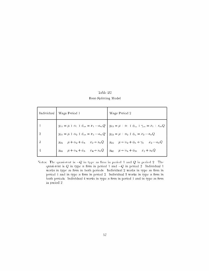
Table B2

Rent-Splitting Model

Individual Wage Period 1 Wage Period 2

1 y11 = �+ �1 + �m = x1 � smQ y12 = �+ �1 + �m + m = x1 + smQ

2 y21 = �+ �2 + �m = x2 � smQ y22 = �+ �2 + �n = x2 � snQ

3 y31 = �+ �3 + �n = x3 + snQ y32 = �+ �3 + �n + n = x3 � snQ

4 y41 = �+ �4 + �n = x4 + snQ y42 = �+ �4 + �m = x2 + snQ

Notes: The quasi-rent is �Q in type m �rm in period 1 and Q in period 2. Thequasi-rent is Q in type n �rm in period 1 and �Q in period 2. Individual 1works in type m �rm in both periods. Individual 2 works in type m �rm inperiod 1 and in type n �rm in period 2. Individual 3 works in type n �rm inboth periods. Individual 4 works in type n �rm in period 1 and in type m �rmin period 2.

57

Table B3

Incentive Model with Heterogeneous Workers

Individual Wage Period 1 Wage Period 2

1 y11 = �+ �1 + �m = w� y12 = �+ �1 + �m + m = w�

2 y21 = �+ �2 + �m = w� y22 = �+ �2 + �m + m = w�

3 y31 = �+ �3 + �m = w� y32 = �+ �3 + �m + m = w�

4 y41 = �+ �4 + �n = y � ��q24 y42 = �+ �4 + �n + n = y + ��2q24 + ��q4

5 y51 = �+ �5 + �n = y � ��q25 y52 = �+ �5 + �n + n = y + ��2q25 + ��q5

6 y61 = �+ �6 + �n = y � ��q26 y62 = �+ �6 + �n + n = y + ��2q26 + ��q6

7 y71 = �+ �7 + �n = y � ��q27 y72 = �+ �7 + �n + n = y + ��2q27 + ��q7

8 y81 = �+ �8 + �n = y � ��q28 y82 = �+ �8 + �n + n = y + ��2q28

9 y91 = �+ �9 + �n = y � ��q29 y92 = �+ �9 + �n + n = y + ��2q29

Notes: Individuals 1, 2, 3 belong to type m �rm with qi, i = 1; 2; 3 between 0 and1/3, individuals 4 to 9 belong to type n �rm with qi, i = 4 to 9 above 1=3.Individuals 4, 5, 6, 7 pass the test and receive the bonus; individuals 8 and 9fail.

58

References

[1] Abowd, John M. (1990) \Does Performance-Based Managerial Compen-sation A�ect Corporate Performance," Industrial and Labor Relations Re-

view, 43:S52-S73, February.

[2] Abowd, John M and Francis Kramarz. (1993) \A Test of Negotiationand Incentive Compensation Models Using Longitudinal French EnterpriseData," In J.C. van Ours, G.A. Pfann, and G. Ridder, editors, Labour De-mand and Equilibrium Wage Formation, (Amsterdam: North-Holland).

[3] Abowd, John M. and Thomas Lemieux. (1993) \The E�ects of Prod-uct Market Competition on Collective Bargaining Agreements: The Caseof Foreign Competition in Canada," Quarterly Journal of Economics,435:983-1014, November.

[4] Brown, James N. and Orley Ashenfelter. (1986) \Testing the E�ciency ofEmployment Contracts," Journal of Political Economy, 94:S55-S78, June.

[5] Bulow, Jeremy and Lawrence Summers. (1976) \A Theory of Dual LaborMarkets with Applications to Industrial Policy, Discrimination and Keyne-sian Unemployment," Journal of Labor Economics, 4:376-414, July.

[6] Cahuc, Pierre and Brigitte Dormont. (1992) \Pro�t Sharing: Does It In-crease Productivity and Employment? A Theoretical Model and EmpiricalEvidence on French Micro Data," Universit�e de Paris I Working Paper,92.45.

[7] Cain, Glenn. (1976) \The Challenge of Segmented Labor Market Theo-ries to Orthodox Theory," Journal of Economic Literature, 14:1215-1257,December.

[8] CEREQ-DEP-INSEE \Bilan Formation - Emploi 1986," INSEE Resultat,75.

[9] Chamberlain, Gary. (1984) \Panel Data," in Z. Griliches and M.D. Intril-ligator, eds., Handbook of Econometrics, (Amsterdam: North Holland).

[10] Dickens, William T. and Lawrence F. Katz. (1987) \Inter-Industry WageDi�erences and Industry Characteristics," In Kevin Lang and Jonathan S.Leonard, eds., Unemployment and the Structure of Labor Markets, (Oxford:Basil Blackwell).

[11] Dickens, WilliamT. and Kevin Lang. (1985) \A Test of Dual Labor MarketTheory," American Economic Review, 75:792-805, September.

[12] Ronald G. Ehrenberg, editor. (1990) Do Compensation Policies Matter?,(Ithaca, NY: ILR Press).

59

[13] Ronald G. Ehrenberg and George T. Milkovich. (1987) \Compensation andFirm Performance," In Steven G. Allen et. al., editor, Human Resources

and the Performance of the Firm, pages 87-122, (Madison, WI: IRRA).

[14] Flinn, Christopher (1986) \Wages and Job Mobility of Young Workers,"Journal of Political Economy.

[15] Gibbons, Robert and Lawrence Katz. (1991) \Layo�s and Lemons," Jour-nal of Labor Economics.

[16] Gibbons, Robert and Lawrence Katz. (1992) \Does Unmeasured AbilityExplain Inter-Industry Wage Di�erentials?" Review of Economic Studies,59:515-535.

[17] Gibbons, Robert and Kevin Murphy. (1990) \Relative Performance Evalu-ation for Chief Executive O�cers," Industrial and Labor Relations Review,43:30S-51S, February.

[18] Gibbons, Robert and K.J. Murphy (1992), \Optimal Incentive Contractsin the Presence of Career Concerns: Theory and Evidence," Journal of

Political Economy 100:468-505.

[19] Groshen, Erica. (1991) \Sources of Intra-Industry Wage Dispersion," Quar-terly Journal of Economics

[20] Hart, Oliver and Bengt Holmstr�om. (1987) \A Theory of Contracts," InTruman F. Bewley, editor, Advances in Economic Theory, Fifth World

Congress, pages 71-155, (Cambridge, Cambridge University Press).

[21] Heckman, James J. and G. Sedlacek (1985) \ " Journal of Political Econ-omy.

[22] Hutchens, Robert. (1987) \A Test of Lazear's Theory of Delayed PaymentContracts," Journal of Labor Economics, 5:S153-S170, October.

[23] INSEE (1989) \Echantillon d'entreprises �etat d'avancement" (Paris: IN-SEE, R�epublique Fran�caise, No. 13/G231).

[24] INSEE (1990a) \Echantillon d'entreprises �chier de r�ef�erence del'�echantillon" (Paris: INSEE, R�epublique Fran�caise, No. 06/G231).

[25] INSEE (1990b) \Echantillon d'entreprises mise �a disposition des donn�eesBIC" (Paris: INSEE, R�epublique Fran�caise, No. 10/G231).

[26] INSEE (1990c) \Echantillon d'entreprises mise �a disposition des donn�eesESE" (Paris: INSEE, R�epublique Fran�caise, No. 64/G231).

[27] Jovanovic, Bojan. (1979) \Job Matching and the Theory of Turnover,"Journal of Political Economy.

60

[28] Kramarz, Francis and Patrick Rey (1994) \The Dynamics of Wages," IN-SEE working paper.

[29] Krueger, Alan B. and Lawrence H. Summers. (1988) \E�ciency Wages andthe Inter-Industry Wage Structure," Econometrica, 56:259-293, March.

[30] Lazear, Edward P. (1979) \Why Is There Mandatory Retirement?" Journal

of Political Economy, 87:1261-1284, December.

[31] Jonathan S. Leonard. (1990) \Executive Pay and Firm Performance," In-dustrial and Labor Relations Review, 43:S13-S29, February.

[32] Stephen Machin, Alan Manning, and Costas Meghir. (1993) \DynamicModels of EmploymentBased on Firm Level Panel Data," In J.C. van Ours,G.A. Pfann, and G. Ridder, editors, Labour Demand and Equilibrium Wage

Formation, (Amsterdam: North-Holland).

[33] MacLeod, W. Bentley and James M. Malcomson. (1989) \Implicit Con-tracts, Incentive Compatibility, and Involuntary Unemployment," Econo-metrica, 57:447-480, March.

[34] MaCurdy, Thomas E. and John Pencavel. (1986) \Testing Between Com-peting Models of Wage and Employment Determination in Unionized Mar-kets," Journal of Political Economy, 94:S3-S39, June.

[35] Meron, Monique (1988) \Les Migrations des salari�es de l'�Etat: plus loin deParis, plus pr�es du soleil," Economie et Statistique, 214, Octobre.

[36] Mundlak, Y. (1978) \On the Pooling of Time Series and Cross SectionData," Econometrica, 46.

[37] Murphy, Kevin M. and Robert H. Topel. (1985) \Least Squares with Esti-mated Regressors" Journal of Business and Economic Statistics.

[38] Nickell, Stephen and Sushil Wadhwani. (1991) \Employment Determina-tion in British Industry: Investigations Using Micro-Data," Review of Eco-

nomic Studies, 58:955-970, October.

[39] Pagan, Adrian (1984) \Econometric Issues in the Analysis of Regressionswith Generated Regressors," International Economic Review, 25:21-47,February.

[40] Rosen, Sherwin (1986) \The Theory of Equalizing Di�erences" in O. Ashen-felter and R. Layard, eds. Handbook of Labor Economics, (Amsterdam:North Holland)

[41] Roy, A. D. (1951) \Some Thoughts on the Distribution of Earnings," OxfordEconomics Papers, 3:135-146, June.

61

[42] Sappington, David. (1991) \Incentives in Principal-Agent Relationships,"Journal of Economic Perspectives 5:45-66.

[43] Sche��e, H. (1959) The Analysis of Variance (New York: Wiley).

[44] Shapiro, Carl and Joseph E. Stiglitz. (1984) \Equilibrium Unemploymentas a Worker Discipline Device," American Economic Review, 74:433-444,June.

[45] Thaler, Richard H. (1989) \Anomalies: Interindustry Wage Di�erentials,"Journal of Economic Perspectives, 3:181-193, Spring.

[46] Topel, Robert and Michael Ward (1992) \Job Mobility and the Careers ofYoung Men," Quarterly Journal of Economics, May.

[47] Willis, Robert (1986) \Wage Determinants: A Survey" in O. Ashenfelterand R. Layard, eds. Handbook of Labor Economics, (Amsterdam: NorthHolland), pp. 525-602.

62