ss-aaea journal of agricultural economics welfare reform’s effect on state … · 2014-01-07 ·...

SS-AAEA Journal of Agricultural Economics

Welfare Reform’s Effect on State Public Welfare Budget Shares

By Andrew D. Compton

_____________________________________________________________________________________________

1

Abstract

This article examines the effect of the Personal Responsibility and Work Opportunity Reconciliation Act of

1996 on state budget shares for public welfare programs between 1991 and 2011. The model is a composite of prior

research. In particular, I utilize a balance wheel model adjusted to model budget shares. This model shares many

similarities with prior political economy model. Welfare Reform ended many traditional welfare programs and

created new ones with more restrictions on recipients. Prior research shows that expenditures have fallen for

traditional programs, but little is concluded about new programs and overall expenditures on public welfare

programs as they relate to the total budget. The findings of this research are largely inconclusive, but more data and

stronger tests could confirm or reject the null hypotheses with more robustness.

Acknowledgements: Special thanks to Dr. Richard Shumway, Dr. Jonathan Yoder, and Gregory

Astill of Washington State University for their feedback and guidance. I would also like to thank Dr.

Chris McIntosh of the University of Idaho for assistance with econometric methods. Finally, I would

like to thank Dr. Ray Batina of Washington State University for guidance when choosing my topic and

for assistance on political economic theory.

In 1996, dramatic changes were made to traditional public welfare programs. The Personal

Responsibility and Work Opportunity Reconciliation Act of 1996 (PRWORA) changed the way

in which the federal government and states are involved in welfare. The primary purposes of

welfare reform were to decrease poverty, increase employment, and encourage families to stay

together while providing more flexibility in how states provide assistance (Sawhill, 1995). The

largest change was the ending of Aid to Families with Dependent Children (AFDC) and the

creation of Temporary Assistance for Needy Families (TANF). Essentially, the act ended open

ended funding and created a system in which the federal government provides block-grants to

states to fund welfare (DHHS). Further, it limited the amount of time one could be on welfare

and placed work requirements on many recipients (DHHS). It also resulted in changes to the

Food Stamp Program, child welfare, benefits to legal immigrants, child nutrition programs, and

reduced the Social Services Block Grant (DHHS) while allowing states to implement programs

as they saw fit.

Many researchers have noted that expenditures on traditional welfare programs have fallen

since PRWORA was implemented. In particular, spending on TANF has fallen as a result of the

many restrictions placed on the receipt of welfare. Unfortunately, much of the research focuses

on traditional programs and only acknowledges that other programs have been implemented at

the state level. Hence, we can say little about the state of welfare beyond the traditional

programs. If there are indeed negative consequences as a result of welfare reform, as many note,

then this raises some ethical dilemmas over fairness and equality. In particular, it raises the

need for further reform to the US welfare system that may include more federal government

involvement to ensure equal treatment across states. If states are indeed implementing their

own programs and moving away from traditional welfare, then it raises concerns about people

receiving different benefits based on their state of birth.

The major goal of this research is to determine whether or not welfare reform in 1996




_____________________________________________________________________________________________

2

resulted in states changing their public welfare budget shares such that welfare received a

smaller proportion of the budget after welfare reform when compared to prior years. I will

simultaneously look for relationships between budget allocations and the makeup of the

population, economic indicators, and other relevant characteristics that may affect welfare. If I

find systematic differences across states, then perhaps potential solutions can be formed to

create a more equal system in which the home state does not affect a person’s ability to get

assistance in a time of need.

Literature Review

Ever since welfare reform was passed, the topic has been of much interest among

researchers. Bentele and Nicoli (2012) investigated whether or not the Personal Responsibility

and Work Opportunity Reconciliation Act of 1996 (PRWORA) led to decreases in state level

spending on social welfare, in particular, Temporary Assistance for Needy Families(TANF). The

main purpose of the study was to examine factors that have contributed to declines in welfare

coverage among states. Bentele and Nicoli based their study on previous work showing that the

number of welfare caseloads has declined since 1996. They utilized common predictors of

welfare participation and coverage. Their hypotheses included increasing coverage as

unemployment increases, higher female employment results in higher coverage or no change at

all, wealthier states will have higher coverage, states with republican governors will have larger

decreases in coverage than states with liberal governors, and that the percent of the state

population that is black will affect coverage. Utilizing a Multilevel Model of Change which

allows examinations of change within and across states, the authors suggest that welfare reform

resulted in lower welfare coverage at the state level. While this is an important result, the

authors acknowledged that there were other programs that may be causing the decrease and

even then, much of the decrease is unaccounted for. Future studies should look at spending on

social services as a whole to examine whether spending has shifted to other parts of the budget

in order to determine if welfare reform had the negative effect indicated.

Prior to Bentele and Nicoli, several studies showed that welfare reform resulted in

decreased coverage. De Jong et al. (2007) examined common policies regarding social welfare

adopted across states and whether or not policy stringency diffused across states. The article is

based on rules regarding welfare put out by the Urban Institute and the PRWORA legislation’s

implications. The primary hypotheses were that after welfare reform, states adopted more

stringent policies regarding welfare and that policy changes diffused across states. De Jong et al

utilized factor analysis which leads to measures of policy types. They used data reduction to

find overall trends. Once they reduced the data, they used OLS regression modeling. Their

longitudinal data comes mainly from the Urban Foundation’s “Welfare Rules Databook” which

list policies for all states. In total, they reduced the data to 15 important policies across 50 states

from 1996-2003 for a total of 8 years. This study from De Jong et al. offers an important

summary of changes in policy across states, which is useful when trying to determine what will

impact change in policy. When examining state budgets, this work provides a basis for




_____________________________________________________________________________________________

3

determining how spending on social welfare may have changed in a given state.

Another study by Danielson and Klerman (2008) implied that welfare reform was

responsible for roughly 10% of the decrease in welfare caseloads while 5% was explained by the

economy which leaves much of the decrease in caseloads unexplained. Their study was based

on inconclusive prior work that indicated that welfare reform may have resulted in a decrease

in caseloads. Their study also utilized the legislation itself which gave more authority to states

and restricts access to welfare, all of which suggested decreases in caseloads and welfare

spending. The primary hypothesis was that welfare reform reduced state welfare caseloads.

Secondary hypotheses were that time limits reduce caseloads, benefits declining with increases

in income reduce caseloads, penalties for noncompliance reduce caseloads, and finally that

alternated assistance programs reduce caseloads. The authors utilized a difference in differences

model of change where changes in caseloads are dependent on policies. One important point

not covered in their study is the side programs which affect overall spending and may cover the

reduction in TANF participation and spending. Essentially, their study fails to explain whether

or not welfare has been reduced overall which should be covered in the future.

Since PRWORA was partially enacted with the intent of reducing poverty, Li and Upadhyay

(2008) analyze whether or not PRWORA actually reduced poverty in the U.S.. Prior work

indicates that welfare reform may have had an impact on poverty among certain groups, but

the evidence is lacking and should be considered carefully. The authors carefully accounted for

determinants of poverty to determine if welfare reform had an effect. The authors provided

some key variables that may be used to explain poverty rates which should be included in any

model of social welfare spending. Using the poverty rate by itself could be problematic due to

its relationship to dependent variables, but by utilizing the variables provided in their study,

that problem is reduced by using exogenous variables. The authors also provide some

indication of the number of people who seek welfare based on poverty, which could affect state

spending on social services. Ultimately, the authors found little evidence that PRWORA

decreased poverty.

While it is commonly acknowledged that TANF spending has decreased as a result of

PRWORA, little work has been done on whether or not overall welfare spending has decreased.

TANF is one among many programs. PRWORA allows states to spend their block grants as they

see fit with their own restrictions on recipients. While previous research suggests that spending

on welfare programs has decreased, little can actually be said about whether welfare has

decreased as a whole instead of one individual program shrinking. In order to account for

changes in state budget size, welfare will be examined as a percentage of the budget instead of

as a nominal or real value.

Economic Theory

The Personal Responsibility and Work Opportunity Reconciliation Act of 1996 (PRWORA)

altered the way in which welfare funds are allocated to states. In particular, the federal

government halted open ended funding for welfare and implemented a block grant system in




_____________________________________________________________________________________________

4

which states receive a fixed amount, which they can choose to do with as they wish. The largest

portion is the switch from Aid to Families with Dependent Children (AFDC) to Temporary

Assistance for Needy Families (TANF). The changes limit welfare receipt to five years over the

course of a person’s life, create incentives to combine work with welfare, require recipients to

participate in work or training at the risk of losing welfare, and allow states to add further

restrictions as they see fit (Martin and Caminada, 2011; Danielson and Klerman, 2009;

Kassabian, Whitesell, and Huber, 2012). Several authors have concluded that poverty has not

been reduced as a result of PRWORA and the switch to TANF has resulted in less funding for

social welfare and fewer applicants for welfare; however, no work has been done on how state

budget allocations have been impacted by PRWORA. If funding for social welfare has fallen as

research has shown, then it is likely that the percentage of the budget that is allocated to public

welfare also decreased, but one must control for changes in the size of the budget and as well as

other relevant variables that impact allocations as well.

The empirical model and variables will be largely based on prior work by Baicker (2001)

who utilizes a political economy model to estimate government expenditures on various

programs. Her model is based on the median voter maximizing their utility by choosing

transfer levels subject to a state government budget constraint. This constraint is specified as tax

revenue being equivalent to expenditures in the form of transfers. Baicker also includes a

constraint specifying changes in intergovernmental transfers. Delaney and Doyle (2011) use a

similar balance wheel model that focuses primarily on education expenditures, but is still based

on a political economy model that maximizes voter utility. I will use a combination of variables

from both models to estimate the effects of welfare reform. Ultimately, state expenditures are

dependent on variables such as unemployment and income which can positively and negatively

impact the median voter and their preferences for who receives welfare. Various demographic

variables that represent the median voter are also considered as well as various shocks such as

changes in the government’s ideology, recessions, and of course, changes in how welfare is

provided at the state level.

The most important variables for consideration in how states allocate their budget are

economic indicators (Bentele and Nicoli, 2012). Thus, consideration will be made for state

unemployment and per capita income. Since welfare spending is primarily dependent on

unemployment, this variable must be taken into consideration. If unemployment increases, then

we would expect to see an increase in demand for public welfare programs such as food stamps

and unemployment insurance. The median voter would also be more supportive of these

programs as the likelihood that they may need welfare could increase. Although per capita

income is a more common measure of income, median income may better reflect the median

voter’s income, particularly with the potential for rising inequality to skew per capita income

disproportionately upward. A lower median income would decrease the median voters ability

to provide for themselves which should increase their support for welfare programs that they

could benefit from.

An important set of independent variables to consider are demographic statistics. As

Baicker notes, the median voter cares about who receives public welfare assistance. In




_____________________________________________________________________________________________

5

particular, they prefer recipients to be similar to themselves so as to ensure that they can receive

welfare should they need it (Baicker, 2001). Further, certain groups will be more likely to need

public welfare. African Americans tend to utilize welfare more than other races, so they have a

significant impact on welfare participation and as a result, one can expect more spending on

social welfare with increasing African American populations (Soss et al, 2001; Wacquant, 2009).

An increasing percentage also increases the likelihood that the median voter is African

American which increases their support for welfare. It would also not be unreasonable to

include the percentage of the population that is Hispanic since they are a large minority of the

population and may not have the same characteristics as other demographics, so they may have

an impact on welfare spending. Another factor to consider is the number of children and elderly

(Baicker 2001).

Since TANF implies that a recipient has children, then it can be anticipated that more

children as a percentage of the population implies more welfare spending. There are also some

programs that provide assistance only to children. The number of children also correlates with

the amount spent on education which affects budget allocations. Further, assuming the median

voter has children or would like children, it can be assumed that they will support more

funding for welfare if it benefits children. On the other hand, more elderly implies that there are

fewer working aged individuals. It also impacts the ideals of the median voter. Another

demographic variable to consider is the percentage of women who work since a working

mother may require more child services and they will be eligible to receive welfare thus

correlating with the amount spent on education and social welfare (Bentele and Nicoli, 2012);

however, inclusion of this variable will depend on locating good data.

Another demographic variable to consider is the dropout rate which is correlated with

poverty and welfare use, so higher dropout rates should result in higher budget allocations to

social welfare programs (Li and Upadhyay, 2009). Unfortunately, dropout rates can be difficult

to attain, but the percentage of the population with a secondary degree and the percentage with

a bachelor’s degree can be used as proxies. Delaney and Doyle (2011) found a relationship

between welfare expenditure and these two variables since higher percentages for both should

decrease welfare use and in turn welfare expenditure; however, a more educated populace may

be more supportive of those experiencing poverty, so the median voter may get utility from

increased public welfare expenditure despite the decrease in their own personal need for public

welfare programs.

Final variables for consideration include political affiliations of the state government, the

size of the total budget, and the voter turnout rate. One should consider the political makeup of

a state since the Republican and Democratic parties differ on how they believe the state budget

should be allocated (Bentele and Nicoli, 2012; Delaney and Doyle, 2011). In particular, the

governor’s party will be considered since the governor has budget authority at the state level

and has the power to veto budgets put forth by the legislature. The size of the total budget will

affect the allocations since some aspects of the budget are fixed and cannot be changed unlike

other aspects. Thus, an increase in the size of the budget could allow for more spending on

public welfare. Finally, voter turnout rates will be considered since it can impact the way




_____________________________________________________________________________________________

6

politicians behave. In particular, if voter turnout rates are low, they may become more

ideological than if rates are high (Delaney and Doyle, 2011). Hence, I would expect lower voter

turnout rates to lead to more drastic changes in welfare programs. Voter turnout rates also

affect the odds that various demographics are represented by the median voter and in turn the

support for public welfare programs.

Previous research has largely concluded that, with a few exceptions, spending on TANF has

decreased since PRWORA went into effect (Hahn, Golden, and Stanczyk, 2012; Bentele and

Nicoli, 2012). Research has also shown that PRWORA decreased caseloads, albeit very little

(Danielson and Klerman, 2008). Combined, these results suggest that welfare reform has

decreased state spending on TANF and traditional welfare programs, but say little about how

budget shares have changed. Another implication is that Republican states should spend less on

social services as a portion of the budget while Democratic states should spend more as a

portion of the state budget based on careful reasoning and prior research showing that this

variable impacts poverty and in turn need for welfare. Finally, based on research and logical

reasoning, demographic, economic, and educational variables should impact budgetary

allocations.

Empirical Model

The empirical model will include each budget category as a dependent variable with all

other variables as the independent variables. The functional form of this model is based on prior

research previously mentioned. In particular, it will closely follow the model used by Delaney

and Doyle (2011) except public welfare expenditures will be specified as a share of the budget.

This model is also very similar to the political economy model built by Baicker (2001). I will

estimate a panel level generalized least squares model (GLS) to account for heteroskedasticity

and autocorrelation if they are present. I expect that both will be present and will estimate a

model using an AR1 autocorrelation structure and then estimate a model with a panel-specific

AR1 autocorrelation structure.

The model is as follows:

Yit = b0t + b1RMIit + b2Uit + b3Age17it + b4Age65it + b5Blackit + b6Hispit + b7Voteit + b8HSit

+ b9Bachit + b10LNRevit + b11Recit + b12RepGovit + b13PRWORAit + eit

With 1 ≤ i ≤ 50 representing each of 50 states and 1991 ≤ t ≤ 2010 representing each of 20

years of data. The dummy variables include the state governor’s party, RepGov, which is

denoted by 1 for years in which a Republican held the Governor’s seat and 0 for years in which

Democrat held the Governor’s seat, a dummy variable for the Personal Responsibility and Work

Opportunity Reconciliation Act of 1996 (PRWORA) where 1 denotes years after 1996 and 0

represents years before 1997, and a dummy variable for recessions, Rec, where 1 denotes

recession years and 0 denotes non-recession years. RMI denotes real median income while U




_____________________________________________________________________________________________

7

represents yearly average unemployment rate. Age17 and Age65 represent the percentage of

the population between the ages of 5 and 17 and the percentage of the population 65 and older

respectively. Black and Hisp represent the percentage of the population that is Black and

Hispanic respectively. Vote represents smoothed voter turnout in the prior year. Smoothing

was achieved by calculating the average slope from two previous years and one coming year

,excluding presidential elections, and then using the slope to calculate the missing third year.

HS and Bach represent the percentage of the population with secondary degrees and bachelor’s

degrees respectively. LNRev represents the natural log of real revenue. It was put in logarithmic

form to make it linear in the parameter as real revenue had a curve in the data when graphed in

relation to public welfare expenditure as a percent of the budget. Finally, e represents a vector

of error terms. Each variable constitutes an it x 1 vector with it totaling to 1000. All real values

are indexed with the consumer price index (CPI) where 1982-84 equals 100.

In order to test the primary hypothesis that PRWORA reduced state level spending on social

welfare programs as the evidence suggests, the model includes a dummy variable for before

and after the act went into place as well as a dependent variable representing the percent of the

budget devoted to human resources which includes social welfare programs. Thus the

coefficient on the dummy variable for PRWORA should be significantly less than 0 to support

the alternative hypothesis and reject the null hypothesis that PRWORA had no effect or a

positive effect on state budget allocations to human resources. We expect that the coefficient on

the Republican dummy variable for the governor’s party should be less than 0 since

Republicans and Democrats have differing views on public welfare programs with Republicans

being less favorable. If the coefficient is significantly less than 0, then it would support the

alternative hypothesis and reject the null hypothesis that the governor’s party has no affect on

budget allocations to human resources.

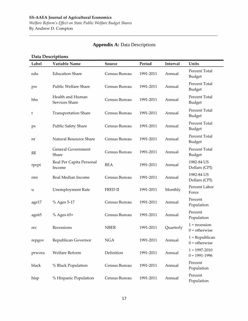
Data

The data for my model is provided by the U.S. Census Bureau, the St. Louis Federal Reserve

Federal Reserve Economic Data (FRED II), National Center for Educational Statistics, National

Bureau of Economic Research, and the National Governor’s Association. For each variable, there

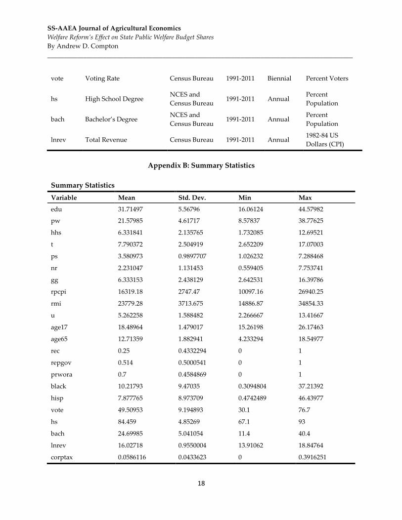
are 20 years of data for each state ranging from 1991 to 2010 for a total of 1000 observations. For

data descriptions and summary statistics, see Appendices A and B. Note that the District of

Columbia is excluded due to its small size, lack of statehood, and the extra influence the federal

government has on its policy.

Annual total and public welfare expenditures for each state provided by the U.S. Census

Bureau will be used to create a budget share proxy (in percent) for public welfare programs.

Total budget expenditures will be indexed with the Consumer Price Index (CPI) provided by

the St. Louis Federal Reserve FRED II with a base year of 1982-84. All expenditure data are for

the fiscal year July 1- June 30. In addition to the expenditure data, total revenue statistics are

provided by the same source and will be treated similarly. Total revenue will be indexed with

the CPI.




_____________________________________________________________________________________________

8

Data on state unemployment rates (in percent of the labor force) are provided by FRED II.

Unemployment rates have been averaged for the year in which expenditures began. Median

income data is provided by the Census Bureau in March of each year. The data is in current

dollars, but is indexed for inflation with the national CPI. Hence, all values are in real 1982-84

dollars.

All demographic data for percent of Blacks, Hispanics, and the age groups are provided by

the U.S. Census Bureau. All data points are intercensal estimates, so they are rebased with each

Census, so there may be some large variation at the end of each decade. The data includes the

percent of the population that is Black, Hispanic, aged 5-17, and aged 65 and over respectively.

Voter turnout rates (in percent) are published by the U.S. Census Bureau after each election.

To account for years during which no election occurs, data will be interpolated. Presidential

elections will not be used for interpolation, but primary elections will be interpolated by using a

moving average to attain values for non-election years. Presidential election years have higher

turnouts than primary elections, so these years would skew the estimation upward.

Data on the percentage of the population with high school equivalent educational

attainment and bachelor’s degree respectively is provided by the National Center for

Educational Statistics (NCES). All data ranges between 0 and 100 percent of the population.

There were two years for which data was unavailable, so the data was smoothed by averaging

between the years before and after the missing value.

Recessions are defined by the National Bureau of Economic Research (NBER), so a dummy

variable for recession years is created with 1 representing recession years and 0 representing

non-recession years. Any year with a quarterly recession is considered to be in a recession.

Information on when states had Republican Governors is provided by the National

Governor’s Association (NGA). Years with Republican Governors are denoted with 1 and non-

Republican Governors are denoted with 0 to create a dummy variable. Independent Governors

are treated as Democratic/non-Republican.

Finally, a dummy variable is created to represent years before and after PRWORA was

enacted. Hence years before 1997 are denoted with 0 and years after 1996 are denoted with 1.

This dummy variable will allow me to test my primary hypothesis that PRWORA resulted in

decreased budget shares for public welfare. Data descriptions and summary statistics are

available in Appendices A and B respectively.

Results

Before running any regressions, I first check for the presence of unit roots in the model.

Since each variable has 1000 observations, a Harris-Tzavalis Test is used to test for the presence

of unit roots (Harris and Tzavalis, 1999). The test yields a test statistic for public welfare’s share

of the budget of -3.9253 with a corresponding p-value less than 0.0001 which means that the

null hypothesis that unit roots are present can be rejected at the 0.05 level; however I will still

estimate a first difference model at the end since the number of years (20) is small for having a

meaningful test. It may also be a more likely model since I am using panel data.




_____________________________________________________________________________________________

9

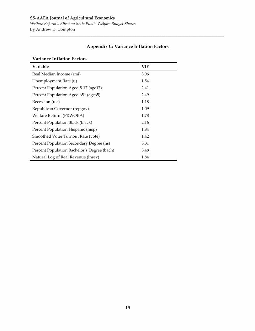
Multicollinearity is the first problem to deal with before running final regressions. To

accomplish this, I check the variance inflation factors (VIFs) for a standard non-panel OLS

regression of Public Welfare on all independent variables. All VIFs (found in Appendix C) are

below 5, so it is reasonable to assume that multicollinearity is not a serious concern.

Before testing for heteroskedasticity and autocorrelation, I first check to see if the panel

model has fixed effects or random effects. To compare the estimates from the random effects

model and fixed effects model, I use a Hausman test with a null hypothesis of non-systematic

differences in coefficients. The chi-squared statistic is 25.40 with a corresponding p-value of

0.0130 which is less than 0.05 so I reject the null hypothesis and estimate a fixed effects model

with systematic differences across models. Thus, further tests will be performed with a fixed

effects model.

Heteroskedasticity is the next problem I check for in the model. For this, I use a modified

Wald Test where the null hypothesis assumes homoskedasticity. The test yields a chi statistic of

2024.27 with a corresponding p-value less than 0.0001. Thus, the null hypothesis is rejected at

the 0.05 level, and I conclude that heteroskedasticity is present in the model. Corrections will be

made for heteroskedasticity depending on whether or not autocorrelation is present in the

model.

Autocorrelation is the final problem I check for in the model before running some final

regressions. To detect the presence of first-order autocorrelation, I use a Wooldridge Test with a

null hypothesis of no first-order autocorrelation. The test yields an F-statistic of F(1, 49) = 80.051

with a corresponding p-value less than 0.0001. Thus, I reject the null hypothesis at the 0.05 level

and conclude that first-order autocorrelation is present in the model. Since both

heteroskedasticity and first-order autocorrelation are present in the model, a GLS regression

will be used to correct the model. Heteroskedasticity will be corrected by transforming the data.

I will estimate the model first with an AR1 autocorrelation structure and then with a panel

specific AR1 autocorrelation structure. If the panel specific AR1 autocorrelation structure

reduces the standard errors, then I will use this structure for the final model.

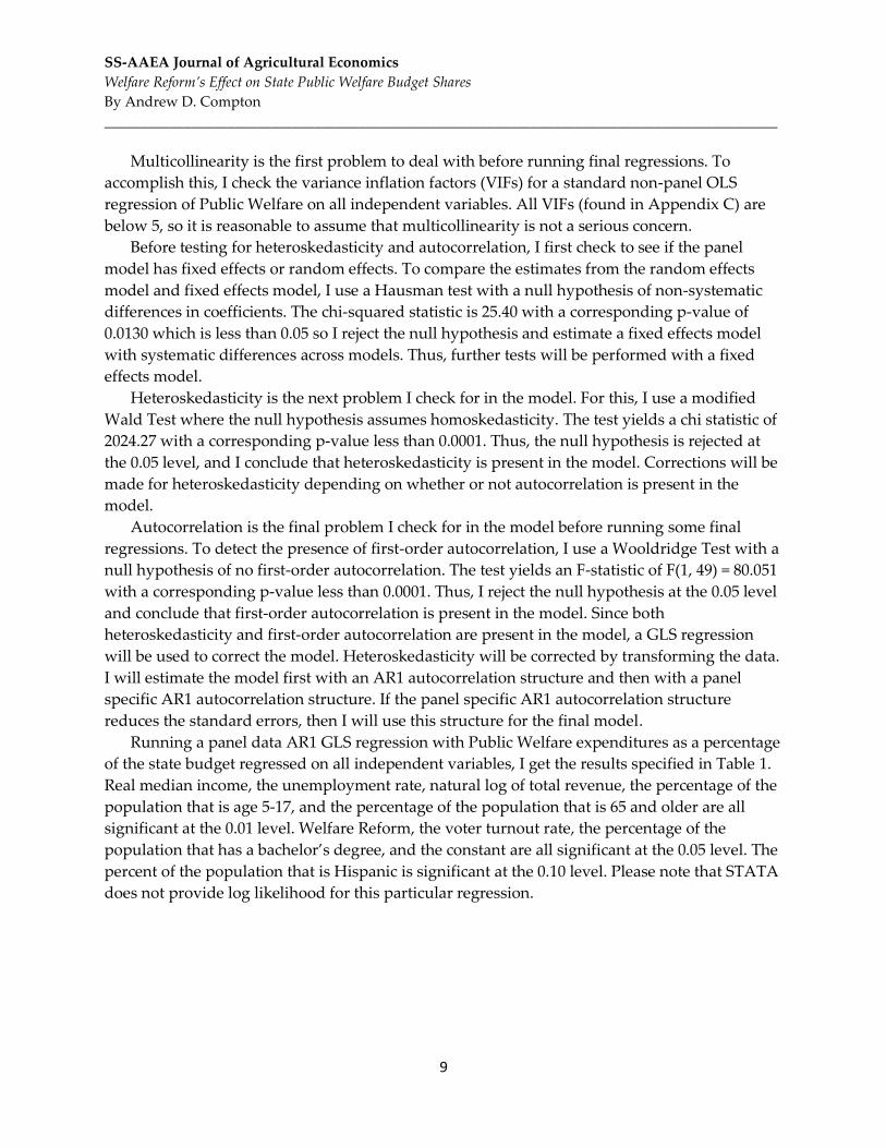
Running a panel data AR1 GLS regression with Public Welfare expenditures as a percentage

of the state budget regressed on all independent variables, I get the results specified in Table 1.

Real median income, the unemployment rate, natural log of total revenue, the percentage of the

population that is age 5-17, and the percentage of the population that is 65 and older are all

significant at the 0.01 level. Welfare Reform, the voter turnout rate, the percentage of the

population that has a bachelor’s degree, and the constant are all significant at the 0.05 level. The

percent of the population that is Hispanic is significant at the 0.10 level. Please note that STATA

does not provide log likelihood for this particular regression.




_____________________________________________________________________________________________

10

Table 1. Panel Data GLS for Public Welfare Expenditure as a Percentage of Budget (PW) AR1 autocorrelation structure

Independent Variable Estimated Coefficient Standard Error p-value

Real Median Income (rmi) -0.00011 0.00003 0.001***

Unemployment Rate (u) 0.19708 0.04846 0.000***

Percent Population Aged 5-17 (age17) -0.42633 0.11389 0.000***

Percent Population Aged 65+ (age65) 0.53988 0.10225 0.000***

Recession (rec) -0.09620 0.10174 0.344

Republican Governor (repgov) -0.14516 0.14174 0.306

Welfare Reform (PRWORA) 0.40715 0.18042 0.024**

Percent Population Black (black) 0.03154 0.01965 0.109

Percent Population Hispanic (hisp) 0.03914 0.02175 0.072*

Smoothed Voter Turnout Rate (vote) 0.01010 0.00456 0.028**

Percent Population Secondary Degree (hs) -0.02069 0.02689 0.442

Percent Population Bachelor’s Degree (bach) 0.06456 0.02619 0.014**

Natural Log of Real Revenue (lnrev) 0.70755 0.17114 0.000***

Constant 11.19479 4.86670 0.021**

Chi Squared 272.18 p-value 0.0000

Number of Observations 1000

Rho 0.7953

***Significant at α=0.010, **Significant at α=0.050, *Significant at α=0.100

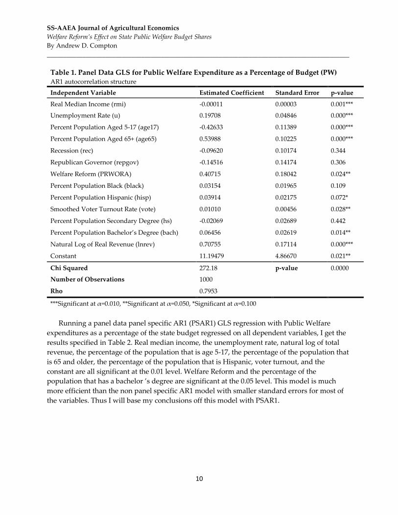
Running a panel data panel specific AR1 (PSAR1) GLS regression with Public Welfare

expenditures as a percentage of the state budget regressed on all dependent variables, I get the

results specified in Table 2. Real median income, the unemployment rate, natural log of total

revenue, the percentage of the population that is age 5-17, the percentage of the population that

is 65 and older, the percentage of the population that is Hispanic, voter turnout, and the

constant are all significant at the 0.01 level. Welfare Reform and the percentage of the

population that has a bachelor ’s degree are significant at the 0.05 level. This model is much

more efficient than the non panel specific AR1 model with smaller standard errors for most of

the variables. Thus I will base my conclusions off this model with PSAR1.




_____________________________________________________________________________________________

11

Table 2. Panel Data GLS for Public Welfare Expenditure as a Percentage of Budget (PW) PSAR1 autocorrelation structure


Real Median Income (rmi) -0.00012 0.00003 0.000***

Unemployment Rate (u) 0.16517 0.04409 0.000***

Percent Population Aged 5-17 (age17) -0.47332 0.09756 0.000***

Percent Population Aged 65+ (age65) 0.53480 0.08947 0.000***

Recession (rec) -0.14931 0.09231 0.106

Republican Governor (repgov) -0.20495 0.12908 0.112

Welfare Reform (PRWORA) 0.38031 0.16209 0.019**

Percent Population Black (black) 0.00142 0.01526 0.926

Percent Population Hispanic (hisp) 0.05733 0.01880 0.002***

Smoothed Voter Turnout Rate (vote) 0.01194 0.00423 0.005***

Percent Population Secondary Degree (hs) -0.02027 0.02484 0.414

Percent Population Bachelor’s Degree (bach) 0.05974 0.02411 0.013**

Natural Log of Real Revenue (lnrev) 0.76517 0.16027 0.000***

Constant 12.36785 4.43349 0.005***




Table 3. Elasticities for GLS with PSAR1 Autocorrelation Structure

Variable Elasticity

Real Median Income -0.1345

Unemployment Rate 0.04028

Percent Population Aged 5-17 -0.4055

Percent Population Aged 65+ 0.3151

Percent Population Hispanic 0.02093

Smoothed Voter Turnout Rate 0.02740

Percent Population Bachelor’s Degree 0.06838

Natural Log of Real Revenue 0.7652

The point elasticities for each variable are calculated in Table 3 above using the average

values. All elasticities are inelastic. A 1percent increase in real median income, unemployment,

voter turnout, and real revenue result in a 0.1345 percent decrease, 0.04028 percent increase,




_____________________________________________________________________________________________

12

0.02740 percent increase, and 0.7652 percent increase in the budget share for public welfare

respectively. Similarly, a 1 percent increase in the percentage of the population aged 5-17, 65+,

percentage of the population Hispanic, and percent of the population with a bachelor’s degree

result in a 0.4055 percent decrease, 0.3151 percent increase, 0.02093 percent increase, and a

0.06838 percent increase in the budget share for public welfare respectively. The elasticity for

the percent of the population that is aged 5-17 is interesting because it suggests that an increase

in the percent of the population that is aged 5-17 results in a large decrease in the budget share

for public welfare. This could be explained by the large number of programs meant to benefit

workers and get them back into the work force or the fact that children cannot vote. Similarly,

the elasticity on the 65+ population is interesting as it suggests that an increase in the elderly

population results in a large increase in the budget share for public welfare. Perhaps this is due

to many elderly having low income, or perhaps it is due to high voter turnout among the

elderly. Finally, in the years after PRWORA was implemented, states devoted 0.3803139 percent

more of their budget to public welfare holding all else constant; however we assume this is 0

since it is not significant at the 0.05 level.

Now, I estimate a GLS model with the data transformed into first difference form in order to

check the robustness of my results should there be a unit root problem present. There is no

evidence of multicollinearity, but tests suggest that there is autocorrelation and

heteroskedasticity. The results of this estimation are provided in Table 4 with the coefficients

on the change model variables being far less significant than in the non-transformed model;

however, since the unit root test is problematic, I do not feel comfortable choosing one model

over another. Especially considering that the change model supports my hypotheses but the

other model rejects them.




_____________________________________________________________________________________________

13

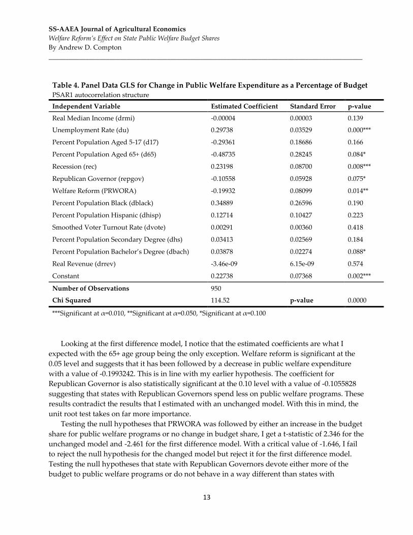
Table 4. Panel Data GLS for Change in Public Welfare Expenditure as a Percentage of Budget PSAR1 autocorrelation structure


Real Median Income (drmi) -0.00004 0.00003 0.139

Unemployment Rate (du) 0.29738 0.03529 0.000***

Percent Population Aged 5-17 (d17) -0.29361 0.18686 0.166

Percent Population Aged 65+ (d65) -0.48735 0.28245 0.084*

Recession (rec) 0.23198 0.08700 0.008***

Republican Governor (repgov) -0.10558 0.05928 0.075*

Welfare Reform (PRWORA) -0.19932 0.08099 0.014**

Percent Population Black (dblack) 0.34889 0.26596 0.190

Percent Population Hispanic (dhisp) 0.12714 0.10427 0.223

Smoothed Voter Turnout Rate (dvote) 0.00291 0.00360 0.418

Percent Population Secondary Degree (dhs) 0.03413 0.02569 0.184

Percent Population Bachelor’s Degree (dbach) 0.03878 0.02274 0.088*

Real Revenue (drrev) -3.46e-09 6.15e-09 0.574

Constant 0.22738 0.07368 0.002***




Looking at the first difference model, I notice that the estimated coefficients are what I

expected with the 65+ age group being the only exception. Welfare reform is significant at the

0.05 level and suggests that it has been followed by a decrease in public welfare expenditure

with a value of -0.1993242. This is in line with my earlier hypothesis. The coefficient for

Republican Governor is also statistically significant at the 0.10 level with a value of -0.1055828

suggesting that states with Republican Governors spend less on public welfare programs. These

results contradict the results that I estimated with an unchanged model. With this in mind, the

unit root test takes on far more importance.

Testing the null hypotheses that PRWORA was followed by either an increase in the budget

share for public welfare programs or no change in budget share, I get a t-statistic of 2.346 for the

unchanged model and -2.461 for the first difference model. With a critical value of -1.646, I fail

to reject the null hypothesis for the changed model but reject it for the first difference model.

Testing the null hypotheses that state with Republican Governors devote either more of the

budget to public welfare programs or do not behave in a way different than states with




_____________________________________________________________________________________________

14

Democrat Governors, I get a t-statistic of -1.588 for the unchanged model and -1.781 for the first

difference model. With a critical value of -1.646, I fail to reject the null hypothesis for the

unchanged model but reject it for the first difference model. This lends increased significance to

the unit root test. Since the sample is small, the unit root test may be biased and could be the

difference between rejecting or accepting my null hypotheses. I am, however, inclined to accept

the first difference model since I would expect panel data to have unit roots. The first difference

model would allow me to conclude that welfare reform and Republican Governors decrease

public welfare expenditure, but more data or stronger tests are needed to reach a conclusion.

Conclusion

The results from the models are inconclusive. While I am able to reject the null hypotheses

in one model, I cannot do so for the other model. With more data, the unit root test would be

stronger and provide a more robust answer to which model to use. While the first difference

model does confirm my hypotheses, I cannot accept the results since they are contradicted by

the other model.

If states are decreasing their expenditures on traditional welfare programs like TANF, they

may very well be transitioning to providing other public welfare services and increasing budget

shares for public welfare programs. Increasingly, states are providing work programs and other

opportunities that help the poor gain employment. They are also increasing spending on

children that is not provided through traditional programs funded by the federal government.

Essentially, states may be spending more on public welfare in ways that they see fit and less on

programs funded by the federal government which has more control over how welfare is

provided even though those programs have given states more control.

The results for the effect of Republican Governors on state budget shares for public welfare

are not significant, but do suggests that the relationships may very well be as I expected. In

further research, perhaps the party affiliation of the legislature should be considered instead

since they do have some control over the budget. The status of the legislature may also better

reflect the overall political climate in each particular state since the legislature has many

members and may better reflect the population’s beliefs assuming that gerrymandering does

not skew representation by a disproportionate amount.

If welfare spending has not changed or has decreased since welfare reform in 1996, then this

would justify looking into whether or not spending is more effective than in the past. I have not

covered the impact of new programs on employment outcomes, but there is ample research on

this topic. Outcomes after welfare reform compared to outcomes prior to welfare reform would

give some indication of whether or not welfare reform has had its intended effect of increasing

employment and decreasing poverty. Unfortunately, it does not appear that expenditures have

had the intended effects meaning that there is still room to increase the efficiency of welfare

expenditures at the current level or increase expenditure. I would encourage a re-evaluation of

the effectiveness of welfare expenditures and reform in the future.

For further research, I would strongly suggest more data and more robust unit root testing




_____________________________________________________________________________________________

15

to determine the actual model. While I modeled state budget shares, it may be better to estimate

per capita budget expenditures for each category and then estimate budget shares. Further, a

seemingly unrelated regression model may account for cross equation correlation among

different budget categories. This may provide better estimates for the variables. To truly

understand its impact, research should shift focus away from traditional programs to analyzing

newer programs that may have been created at the state level following PRWORA. These

programs may give us a better understanding of the ways in which PRWORA affected public

welfare expenditures and budget shares.

References

Baicker, K. 2001. “Government decision-making and the incidence of federal mandates.” Journal of Public

Economic, 82:147-194.

Bentele, K.G. and L.T. Nicoli. 2012. “Ending Access as We Know It: State Welfare Benefit Coverage in the

TANF Era.” Social Service Review 86:223-268.

Danielson, C. and J.A. Klerman. 2008. “Did Welfare Reform Cause the Caseload Decline.” Social Service

Review 82:703-730.

De Jong, G.F., D.R. Graefe, S.K. Irving, and T. St. Pierre. 2006. “Measuring State TANF Policy Variations

and Change After Reform.” Social Science Quarterly 87:755-781.

Delaney, J.A. and W.R. Doyle. 2011. “State Spending on Higher Education: Testing the Balance Wheel

over Time.” Journal of Education Finance 36: 343-368.

Dept. of Health and Human Services. April 1997. “Major Provisions of the Personal Responsibility and

Work Opportunity Act of 1996.” Findlaw.com. Available online at:

<http://corporate.findlaw.com/law-library/major-provisions-of-the-personal-responsibility-and-

work.html>.

Federal Reserve Economic Data. [2013]. CPIAUCSL: Consumer Price Index for All Urban Consumers: All

Items [Data]. Available from http://research.stlouisfed.org/fred2/series/CPIAUCSL/downloaddata

Federal Reserve Economic Data. [2013]. Unemployment Rate [Data]. Availabel from

http://research.stlouisfed.org/

Granger, C.W.J. and P. Newbold. 1974. “Spurious Regressions in Economics.” Journal of Econometrics

2:111-120.

Hahn, H., O. Golden, and A. Stanczyk. 2012. “State Approaches to the TANF Block Grant: Welfare Is Not

What You Think It Is.” The Urban Institute, Working Families Paper 20.

Harris, R.D.F. and E. Tzavalis. 1999. “Inference for unit roots in dynamic panels where the time

dimension is fixed.” Journal of Econometrics 91:201-226.

Hines Jr., J.R. 2006. “Will Social Welfare Expenditures Survive Tax Competition.” Oxford Review of

Economic Policy 22:330-348.

Kassabian, D., A. Whitesell, and E. Huber. 2011. “Welfare Rules Databook: State TANF Policies as of July

2011.” Office of Planning, Research and Evaluation, U.S. Department of Health and Human Services,

Report 2012-57.

Li, H. and M. Upadhyay. 2008. “Has the 1996 Welfare Reform Reduced the U.S. Poverty Rate? An

Emperical Analysis Using Panel Data.” Economics Bulletin 9:1-8.

Martin, M.C. and K. Caminada. 2011. “Welfare Reform in the U.S.: A Policy Overview Analysis.” Poverty

and Public Policy 3:Article 8.




_____________________________________________________________________________________________

16

National Bureau of Economic Research. (2010). US Business Cycle Expansions and Contractions [Text].

Available from http://www.nber.org/cycles.html

National Center for Education Statistics. (2012). Dropouts, Completers, and Graduation Rate Reports [Data

Files]. Available from http://nces.ed.gov/pubsearch/getpubcats.asp?sid=001

National Governor’s Association. (2013). Governors: Listed by State [Text]. Available from

http://www.nga.org/portal/site/nga/menuitem.5dbb9333fc52447ae8ebb856a11010a0

Sawhill, I.V. 1999. “Welfare Reform: An Analysis of the Issue.” The Urban Institute, available from

http://www.urban.org/publications/306620.html

Soss, J., S.F. Schram, T.P. Vartanian, and E. O’Brien. 2001. “Setting the Terms of Relief: Explaining State

Policy Choices in the Devolution Revolution.” American Journal of Political Science 45:378-395.

U.S. Census Bureau. (2001). Population Estimates: 1990s: State Tables [Data]. Available from

http://www.census.gov/popest/data/historical/1990s/state.html

U.S. Census Bureau. (2012). Population Estimates: State Intercensal Estimates(2000-2010) [Data]. Available

from http://www.census.gov/popest/data/intercensal/state/state2010.html

U.S. Census Bureau. (2011). State Government Finances: 1992-2011 [Data]. Available from

http://www.census.gov/govs/state/historical_data.html

U.S. Census Bureau. (2011). State Median Income: Median Household Income by State – Single Year Estimates

[Data]. Available from http://www.census.gov/govs/state/historical_data.html

U.S. Census Bureau. (2012). Voting and Registration [Data Files]. Available from

http://www.census.gov/hhes/www/socdemo/voting/publications/historical/index.html

Wacquant, L. 2009. “Punishing the Poor: The Neoliberal Government of Social Insecurity.”

Durham, NC: Duke University Press.




_____________________________________________________________________________________________

17

Appendix A: Data Descriptions

Data Descriptions

Label Variable Name Source Period Interval Units

edu Education Share Census Bureau 1991-2011 Annual Percent Total

Budget

pw Public Welfare Share Census Bureau 1991-2011 Annual Percent Total

Budget

hhs Health and Human

Services Share Census Bureau 1991-2011 Annual

Percent Total

Budget

t Transportation Share Census Bureau 1991-2011 Annual Percent Total

Budget

ps Public Safety Share Census Bureau 1991-2011 Annual Percent Total

Budget

nr Natural Resource Share Census Bureau 1991-2011 Annual Percent Total

Budget

gg General Government

Share Census Bureau 1991-2011 Annual

Percent Total

Budget

rpcpi Real Per Capita Personal

Income BEA 1991-2011 Annual

1982-84 US

Dollars (CPI)

rmi Real Median Income Census Bureau 1991-2011 Annual 1982-84 US

Dollars (CPI)

u Unemployment Rate FRED II 1991-2011 Monthly Percent Labor

Force

age17 % Ages 5-17 Census Bureau 1991-2011 Annual Percent

Population

age65 % Ages 65+ Census Bureau 1991-2011 Annual Percent

Population

rec Recessions NBER 1991-2011 Quarterly 1 = recession

0 = otherwise

repgov Republican Governor NGA 1991-2011 Annual 1 = Republican

0 = otherwise

prwora Welfare Reform Definition 1991-2011 Annual 1 = 1997-2010

0 = 1991-1996

black % Black Population Census Bureau 1991-2011 Annual Percent

Population

hisp % Hispanic Population Census Bureau 1991-2011 Annual Percent

Population




_____________________________________________________________________________________________

18

vote Voting Rate Census Bureau 1991-2011 Biennial Percent Voters

hs High School Degree NCES and

Census Bureau 1991-2011 Annual

Percent

Population

bach Bachelor’s Degree NCES and

Census Bureau 1991-2011 Annual

Percent

Population

lnrev Total Revenue Census Bureau 1991-2011 Annual 1982-84 US

Dollars (CPI)

Appendix B: Summary Statistics

Summary Statistics

Variable Mean Std. Dev. Min Max

edu 31.71497 5.56796 16.06124 44.57982

pw 21.57985 4.61717 8.57837 38.77625

hhs 6.331841 2.135765 1.732085 12.69521

t 7.790372 2.504919 2.652209 17.07003

ps 3.580973 0.9897707 1.026232 7.288468

nr 2.231047 1.131453 0.559405 7.753741

gg 6.333153 2.438129 2.642531 16.39786

rpcpi 16319.18 2747.47 10097.16 26940.25

rmi 23779.28 3713.675 14886.87 34854.33

u 5.262258 1.588482 2.266667 13.41667

age17 18.48964 1.479017 15.26198 26.17463

age65 12.71359 1.882941 4.233294 18.54977

rec 0.25 0.4332294 0 1

repgov 0.514 0.5000541 0 1

prwora 0.7 0.4584869 0 1

black 10.21793 9.47035 0.3094804 37.21392

hisp 7.877765 8.973709 0.4742489 46.43977

vote 49.50953 9.194893 30.1 76.7

hs 84.459 4.85269 67.1 93

bach 24.69985 5.041054 11.4 40.4

lnrev 16.02718 0.9550004 13.91062 18.84764

corptax 0.0586116 0.0433623 0 0.3916251




_____________________________________________________________________________________________

19

Appendix C: Variance Inflation Factors

Variance Inflation Factors

Variable VIF

Real Median Income (rmi) 3.06

Unemployment Rate (u) 1.54

Percent Population Aged 5-17 (age17) 2.41

Percent Population Aged 65+ (age65) 2.49

Recession (rec) 1.18

Republican Governor (repgov) 1.09

Welfare Reform (PRWORA) 1.78

Percent Population Black (black) 2.16

Percent Population Hispanic (hisp) 1.84

Smoothed Voter Turnout Rate (vote) 1.42

Percent Population Secondary Degree (hs) 3.31

Percent Population Bachelor’s Degree (bach) 3.48

Natural Log of Real Revenue (lnrev) 1.84

ss-aaea journal of agricultural economics welfare reform’s effect on state … · 2014-01-07 ·...

Documents