s.s.b.com ii macro economic issues and policies unit 1 …

S.S.B.COM IIMACRO ECONOMIC ISSUES AND POLICIES

UNIT 1THE QUANTITY THEORY OF MONEY: THE

CLASSICAL AND NEO CLASSICAL VIEW

DEPARTMENT OF BUSINESS ECONOMICS

FACULTY OF COMMERCE, MSU

Dept. of Business Economics, FoC, M.S. University of Baroda 1

Theories of Money and Prices

• Classical Quantity Theory of Money– Different Versions

• Keynes’s Critique and Keynesian Theory of Money & Prices

• Friedman’s Restatement of Quantity Theory


The Quantity Theory of Money


The Quantity Theory of Money• Transactions and the Quantity Equation

• People hold money to buy goods and services.

• The more money they need for such transactions, the more money they hold.

• The link between transactions and money is expressed in the following equation, called the quantity equation:

Money × Velocity = Price × Transactions

or, M × V = P × T.

• Examining each of the four variables in this equation:

• The right-hand side of the quantity equation tells us about transactions.

• T represents the total number of transactions during some period of time, say, a year.

• In other words, T is the number of times in a year that goods or services are exchanged for money.

• P is the price of a typical transaction—the number of rupee notes exchanged.

• The product of the price of a transaction and the number of transactions, PT, equals the number of rupee notes exchanged in a year.


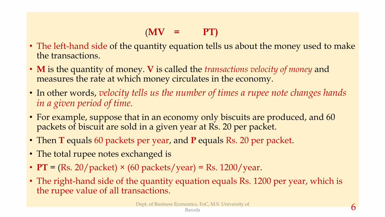
(MV = PT)

• The left-hand side of the quantity equation tells us about the money used to make the transactions.

• M is the quantity of money. V is called the transactions velocity of money and measures the rate at which money circulates in the economy.

• In other words, velocity tells us the number of times a rupee note changes hands in a given period of time.

• For example, suppose that in an economy only biscuits are produced, and 60 packets of biscuit are sold in a given year at Rs. 20 per packet.

• Then T equals 60 packets per year, and P equals Rs. 20 per packet.

• The total rupee notes exchanged is

• PT = (Rs. 20/packet) × (60 packets/year) = Rs. 1200/year.

• The right-hand side of the quantity equation equals Rs. 1200 per year, which is the rupee value of all transactions.


Calculating Velocity

• Suppose further that the quantity of money in the economy is Rs. 600.

• By rearranging the quantity equation, we can compute velocity as

V = PT/M

• = (Rs. 1200/year)/(Rs. 600)

• = 2 times per year.

• That is, for Rs. 1200 of transactions per year to take place with Rs. 600 of

money, each rupee note must change hands 2 times per year.


The Quantity Theory of Money

The theory that increase in the quantity of money leads to the rise in the general

price level was first put forward by Irving Fisher.

Premise: The greater the quantity of money, the higher the level of prices and

vice versa.

Therefore, the theory which linked prices with the quantity of money came to be

known as quantity theory of money.

Stated in its simplest form, the quantity theory of money says that the level of prices

varies directly with quantity of money.

The price level rises proportionately with a given increase in the quantity of money,

other things remaining the same.


• The general price level in a community is influenced by the following factors:

(a) The volume of trade or transactions;

(b) The quantity of money;

(c) Velocity of circulation of money.

• The volume of trade or transactions depends upon the amount of goods and services to

be exchanged.

• This was assumed to be constant as the classical and neoclassical economists subscribing

to the quantity theory of money assumed full employment of all resources in the economy.

• Hence the total (real) volume of trade or transactions would remain the same.

• The quantity of money would be given by the Central monetary authority.

• The velocity of circulation of money, i.e., the number of times a unit of money changes

hands during exchanges in a year, was assumed to be given by institutional factors.Dept. of Business Economics, FoC, M.S. University of

Baroda 9

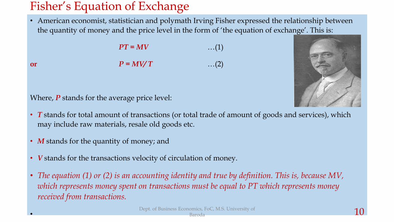
Fisher’s Equation of Exchange• American economist, statistician and polymath Irving Fisher expressed the relationship between

the quantity of money and the price level in the form of ‘the equation of exchange’. This is:

PT = MV …(1)

or P = MV/ T …(2)

Where, P stands for the average price level:

• T stands for total amount of transactions (or total trade of amount of goods and services), which

may include raw materials, resale old goods etc.

• M stands for the quantity of money; and

• V stands for the transactions velocity of circulation of money.

• The equation (1) or (2) is an accounting identity and true by definition. This is, because MV,

which represents money spent on transactions must be equal to PT which represents money

received from transactions.

•Dept. of Business Economics, FoC, M.S. University of

Baroda 10

From Accounting Identity to A Theory of the Price Level• However, the equation of exchange as given in equations (1) and (2) has been converted into a

theory of determination of general level of prices by making the following assumptions.

• 1) The physical volume of transactions (T) is constant.

• 2) The transactions velocity of circulation (V) is also constant in the short run.

• The quantity theorists believed that the volume of transactions (T) and the changes in it were

largely independent of the quantity of money.

• They also believed that changes in velocity of circulation (V) and price level (P) do not cause any

change in volume of transactions except temporarily.

• Thus the Classical proponents of the quantity theory of money believed that the number of

transactions (which ultimately depends on aggregate real output) does not depend on other

variables (M, V and P) in the equation of exchange.

• Thus the assumption of constant V and T converts the equation of exchange (MV =

PT), which is an accounting identity, into a theory of the determination of general price

level. Dept. of Business Economics, FoC, M.S. University of Baroda 11

Prices and the Quantity of Money: Example• The quantity of money is fixed by the Government and the Central Bank of a country, and is

assumed to be autonomous of the real forces which determine the volume of transactions or

national output.

• Now, with the assumptions that M and V remain constant, the price level P depends upon the

quantity of money M; the greater the quantity of M, the higher the level of prices.

• Numerical Example: Suppose the quantity of money is ` 5,00,000 in an economy, the velocity

of circulation of money (V) is 5; and the total output to be transacted (T) is 2,50,000 units. What

will be the average price level (P)?

Now suppose the quantity of money increases to 10,00,000. What will be the new price level other

things remaining the same?

•


The Money-Price Proportionality Relation

The Quantity Theory thus implies that the price level varies in direct proportion to

the quantity of money.

A doubling of the quantity of money (M) will lead to the doubling of the price level.

Further, since changes in the quantity of money are assumed to be

independent or autonomous of the price level, the changes in the

quantity of money become the cause of the changes in the price level.


P = (V/T).M

Quantity Theory of Money: Income Version• The volume of transactions and its average price level referred to in Fisher’s transactions approach

to quantity theory of money are conceptually difficult to measure.

• Therefore, in later approaches the quantity theory was formulated in the income form which

considers real income or GDP (i.e., transactions of final goods only) rather than all transactions.

• Data regarding national income or output is readily available.

• Also, the average price level of output is a more meaningful and useful concept.

• The general price level in a country is measured taking into account only the prices of final goods

and services which constitute national product.

• Note that even in this income version of the quantity theory of money, the function of money is

considered to be a means of exchange as in the transactions approach of Fisher.

• The concept of income velocity of money has been used instead of transactions velocity of circulation.

• By income velocity we mean the average number of times per period a unit of money is used in

making payments involving final goods and services, that is, national product or national income.


The Income Version of the Quantity Theory• The income version of quantity theory of money is written as below:

MV = PY … … (3)

Or, P = MV/Y … … …(4)

Where

• M = Quantity of money

• V = Income velocity of money

• P = Average price level of final goods and services

• Y = Real national income (or aggregate output)

• Like in the transactions approach, in this income version of the quantity theory also, the different

variables are assumed to be independent of each other.

• Further, income velocity of money (V) and real income or aggregate output (Y) are assumed to be

given and constant during a short period. They do not vary in response to the changes in M.Dept. of Business Economics, FoC, M.S. University of Baroda 16

• Real income or output (Y) is assumed to be determined by the real sector forces such as

capital stock, the amount and skills of labour, technology etc.

• These factors are taken to be given in the short run.

• Further, the assumptions of Say’s law and wage-price flexibility ensure full employment

of resources.

Supply of output is inelastic and constant at full-employment level.

• It follows from equations (3) and (4) above that with income velocity (V) and

national output (Y) remaining constant, price level (P) is determined by the

quantity of money (M).


Classical Quantity Theory of Money in the Aggregate Demand-Aggregate Supply Framework

• The quantity of money (M) multiplied by the income velocity of circulation (V), that is, MV gives us aggregate expenditure in the quantity theory of money.

• Now, with a given quantity of money, say M1 and constant velocity of money V , we have a given amount of monetary expenditure (M1V ).

• Given this aggregate expenditure, at a lower (higher) price level more (less) quantities of goods can be purchased and at a higher price level, less quantities of goods can be purchased.

• Therefore, in accordance with classical quantity theory of money aggregate demand, representing M1V slopes downward.

• This is shown by the aggregate demand curve AD1 in Fig. 1 below.


The downward sloping schedule AD1 represents the

aggregate demand corresponding to money supply

M1. If the quantity of money is increased to M2. the

aggregate demand curve, representing new

aggregate monetary expenditure M2V will shift to

the right.

The aggregate supply curve AS is completely

inelastic given the assumptions of perfect wage-

price flexibility and full-employment.

The aggregate demand curve AD1 cuts the

aggregate supply curve AS at point E and

determines price level OP1.

Now, if the quantity of money is increased to M2,

the aggregate demand curve shifts upward to AD2.

With the increase in aggregate demand to AD2,

excess demand (=EB) emerges at the current price

level OP1.

As output cannot be increased, the excess demand

will lead the price level increase to OP2 at which

again aggregate quantity demanded equals the

aggregate supply which remains unchanged at OYF

.

Pri

ce L

evel

Aggregate Demand, Aggregate Supply

O

P2

P1

YF

H

AS

AD1 (M1V)

AD2 (M2V)

E B

Fig. 1: Quantity Theory: Depiction in Aggregate

Demand-Supply FrameworkDept. of Business Economics, FoC, M.S. University of

Baroda 19

Quantity Theory of Money: the Cambridge Cash-balance

Approach• Cambridge economists Marshall and Pigou have stated the equation of exchange in a form

different from Irving Fisher. According to the Cambridge economists, the value of money (i.e., its

purchasing power) is determined by the demand for and supply of money.

• In cash-balance approach to demand for money Cambridge economists laid stress on the store of

value function of money in contrast to the medium of exchange function depicted by Fisher.

• According to cash balance approach, the public likes to hold a proportion of nominal income (k,

say) in the form of money (i.e., cash balances).

• Then cash balance approach can be written as:

• Md = kPY … (1)

• where Y = real national income (i.e., aggregate output), P = the price level

• PY = nominal national income,

• k = the proportion of nominal income that people want to hold in money

• Md = the amount of money which public want to holdDept. of Business Economics, FoC, M.S. University of

Baroda 20

• For equilibrium in the money market, demand for money must equal with the supply of

money, M.

• The supply of money M is exogenously given and is determined by the monetary policies

of the central bank of a country. Thus, for equilibrium in the money market,

M = M d

Or, M = kPY … (2)

k in the equations (1) and (2) is related to velocity of circulation of money V in Fisher’s

transactions approach. Thus, when a greater proportion of nominal income is held in the

form of money (i.e., when k is higher), V falls.

• “The higher the proportion of their real incomes that people decide to keep in

money, the lower will be the velocity of circulation, and vice versa.”

• It follows from above that k = 1/V.


Price Determination

Rearranging equation (2), we have the cash balance equation giving price as the dependent variable,

as

P = (1/k).M/Y …(3)

Like Fisher’s equation, cash balance equation is also an accounting identity because k is defined as:

Quantity of Money / National Income, or, = M/ PY

Now, the Cambridge economists also assumed that k remains constant.

Further, due to their belief that wage-price flexibility would ensure full employment of resources, the

level of real national income was also fixed.

Thus, from equation (3) it follows that with k and Y remaining constant , price level (P) is

determined by the quantity of money (M);

Changes in the quantity of money will cause proportionate changes in the price level.


The Cash balance & the Transactions Approach Compared

There are some similarities between the Cambridge cash-balance approach andFisher’s transactions approach.

• k is reciprocal of V. That is, k = 1/V or V= 1/k

• Thus in equation (2) above, if we replace k by 1/V, we have,

M = (1/V). PY

or MV = PY, which is the income version of Fisher’s quantitytheory of money.

• However, the similarity in form notwithstanding, there are important conceptualdifferences between the two which makes cash-balance approach superior to thetransactions approach. In very brief,

• Fisher’s transactions approach lays stress on the medium of exchange function ofmoney, while the cash balance approach emphasises the store-of-value functionof money.

• Further, the Cambridge explanation of the factors which determine velocity ofcirculation, k in the cash balance approach, is behavioural in nature, unlike themechanistical approach of the transactions version in explaining V.


Criticism of the Quantity Theory by Keynes and his Associates:

1. The theory has been alleged to be a “Useless truism”. With the qualification that velocity

of money (V) and the total output (T) remain the same, the equation of exchange (MV = PT)

is a useless truism.

Fisher’s equation of exchange simply tells us that expenditure made on goods (MV) is equal

to the value of output of goods and services sold (PT).

2. Velocity of money is not stable. Keynesian economists have challenged the QuantityTheory assumption that velocity of money remains stable.

They argue that velocity changes inversely with the change in money supply. Increase inmoney supply, with constant demand for money, leads to the fall in the rate of interestwhich will cause people to hold more money as idle cash balances (under speculativemotive). This means velocity of circulation of money will be reduced.

3. The third criticism is that increase in quantity of money may not always lead to theincrease in aggregate expenditure or aggregate demand.

Note that changes in the quantity of money DO often induce changes in the volume ofaggregate spending. What Keynes and his followers deny is the assertion that there exists adirect, simple, and more or less a proportional relation between variation in money supplyand variation in the level of total spending.Dept. of Business Economics, FoC, M.S. University of

Baroda 24

P4

PF

P0

AD0AD1

AD2

AD3

AD4

YF

Over the horizontal range AE0 on the aggregate supplycurve AS, the economy is in recession, there isunemployment and excess productive capacity. Supplyof output is perfectly elastic over this range.Suppose now that the government seeks to cure thisrecession by increasing spending on infrastructure, andfinances this by printing new money, i.e., byaugmenting money supply.As aggregate demand AD increases to AD1, output canbe expanded to Y1 without any increase in costs andtherefore, prices, by putting into use the excess capacityin the economy. In the short-run, thus, it is output, notprice, that adjusts to an increase in aggregate demand.Over the upwardly sloped range E0E1EF on AS, bothprice and output adjust upwards as aggregate demandincreases, until the full employment output YF isreached.It is only when output reaches full-employment level YF,that further increase in money supply will lead toincrease in the price level in full proportion.

Y2Y1Y0

A E0

EF

Thus, according to Keynes, it is only when the economy is operating at full-employment or potential output level that increase in money supply leads to the proportionate rise in price level.However, full employment cannot be assumed to be a normal state of affairs in a free-market economy.


Criticisms: (contd.)

4. Perhaps the most serious criticism levelled by Keynes against the Quantity

Theory is its envisaged role of money solely as a medium of exchange. That people

may hold money for reasons other than transactions purposes, particularly for

speculative motives, was to be later elegantly formalized in Keynes’s own theory of

the demand for money.

Crowther comments, “The modern tendency in economic thinking, in fact, is to

discard the old notion of the quantity of money as a causative factor in the state of

business and a determinant of the value of money and to regard it as a

consequence”.


Factors Other than Quantity of Money Also Affect the Price Level.

• The quantity theory does not consider other factors than the quantity of money

that cause changes in aggregate demand and influence changes in price level.

• Some of these factors are: increase in government expenditure. with

quantity of money remaining unchanged--- increased investment by optimistic

investors, or increase in demand for exports of a country, all of which cause

aggregate expenditure to increase.

• If the increase in aggregate demand is not matched by sufficient increase in

supply of output, imbalance between demand and supply causes price level to

rise

• Below, we consider just one such instance in economic history when prices rose

exorbitantly in a sustained manner without any change in money supply.


3• Prices may rise due to supply-side

factors, even when the quantity of

money remains the same.

• The stagflation of 1970s is a

remarkable case in point.

• It was caused by the hiking of price of

crude oil by the OPEC countries,

raising cost of production in many

industries and shifting the short-run

aggregate supply curve to the left

(Fig. 3).

• Thus, prices increased steeply even

without increase in the quantity of

money.



"The quantity theory of money thus rests,

ultimately, upon the fundamental

peculiarity which money alone of all

human goods possesses - the fact that it

has no power to satisfy human wants

except a power to purchase things which

do have such power.“

Irving Fisher, Purchasing Power of

Money, 1911: p.32

It is precisely THIScharacterization of moneythat later economists wereto contest and developmore fuller, realistictheories of money.


References:1. Macroeconomics (2003): N. Gregory Mankiw2. Macroeconomics: Theory & Policy (20th Ed.): H. L. Ahuja

s.s.b.com ii macro economic issues and policies unit 1 …

Documents