Published by Scientific technical

Union of Mechanical Engineering “INDUSTRY 4.0”

I n t e r n a t i o n a l j o u r n a l for science, technics andinnovations for the industry

YE

AR

XI

3

Is

su

e

IS

SN

PR

INT

13

13

-02

26

IS

SN

WE

B 1

31

4-5

07

X/

2017

MACHINESTECHNOLOGIESMATERIALS

MACHINES. TECHNOLOGIES. MATERIALS

INTERNATIONAL SCIENTIFIC JOURNAL

PUBLISHER

SCIENTIFIC TECHNICAL UNION OF MECHANICAL ENGINEERING “INDUSTRY 4.0”

108, Rakovski Str., 1000 Sofia, Bulgaria tel. (+359 2) 987 72 90,

tel./fax (+359 2) 986 22 40, office@stumejournals.com www.stumejournals.com

ISSN PRINT 1313-0226, ISSN WEB 1314-507X, YEAR XI, ISSUE 3 / 2017

EDITOR-IN-CHIEF

Prof. D.Sc. DHC Georgi Popov, President of Bulgarian Scientific and Technical Union of Mechanical Engineering

EDITORIAL BOARD

MEMBERS . SCIENTIFIC COMPETENCE Prof. Dimitar Damyanov Automatisation of production

Prof. Dimitar Karaivanov Mechanics of machines Prof. Dimitar Stavrev Technologies and materials

Prof. Dimitar Yonchev National and industrial security Prof. Galina Nikolcheva Machines tools and technologies

Prof. Hristo Shehtov Automatisation of production Prof. Idilija Bachkova Automatisation of production

Prof. Ivan Kralov Mechanics of machines Prof. Ivan Parshorov Technologies and materials

Prof. Ivan Yanchev Machines and technologies Prof. Ivo Malakov Automatisation of production

Prof. Kiril Angelov Industrial Management Prof. Lilo Kunchev Transport Equipment and Technology

Prof. Lubomir Dimitrov Machines and technologies Prof. Miho Mihov Agricultural machinery

Prof. Miroslav Denchev Ergonomics and design Prof. Mladen Velev Economics and Marketing

Prof. Nikolay Diulgerov Technologies and materials Prof. Ognyan Andreev Production management

Prof. Petar Kolev Transport Equipment and Technology Prof. Roman Zahariev Robotics

Prof. Sasho Guergov Robotic systems and technology Prof. Tsanka Dikova Technologies and materials Prof. Vitan Galabov Mechanics of machines

MACHINES. TECHNOLOGIES. MATERIALS

INTERNATIONAL SCIENTIFIC JOURNAL

EDITORIAL BOARD FOREIGN MEMBERS

Prof. Adel Mahmoud IQ Prof. Marian Tolnay SK Prof. Ahmet Ertas TR Prof. Mark Easton AU Prof. Andonaq Londo AL Prof. Mart Tamre EE Prof. Andrei Firsov RU Prof. Maryam Ehteshamzade IR Prof. Andrzej Golabczak PL Prof. Michael Evan Goodsite DK Prof. Anita Jansone LV Prof. Movlazade Vagif Zahid AZ Prof. Aude Billard CH Prof. Natasa Naprstkova CZ Prof. Bojan Dolšak SI Prof. Oana Dodun RO Prof. Christian Marxt LI Prof. Oleg Sharkov RU Prof. Dale Carnegie NZ Prof. Páll Jensson IS Prof. Ernest Nazarian AM Prof. Patrick Anderson NL Prof. Esam Husein KW Prof. Paul Heuschling LU Prof. Ewa Gunnarsson SW Prof. Pavel Kovac RS Prof. Filipe Samuel Silva PT Prof. Per Skjerpe NO Prof. Francisco Martinez Perez CU Prof. Péter Korondi HU Prof. Franz Haas AT Prof. Peter Kostal SK Prof. Genadii Bagliuk UA Prof. Juan Alberto Montano MX Prof. Georg Frey DE Prof. Raul Turmanidze GE Prof. Gregory Gurevich IL Prof. Renato Goulart BR Prof. Haydar Odinaev TJ Prof. Roumen Petrov BE Prof. Hiroyuki Moriyama JP Prof. Rubén Darío Vásquez Salazar CO Prof. Iryna Charniak BY Prof. Safet Isić BA Prof. Ivan Svarc CZ Prof. Sean Leen IE Prof. Ivica Veza HR Prof. ShI Xiaowei CN Prof. Jae-Young Kim KR Prof. Shoirdzan Karimov UZ Prof. Jerzy Jedzejewski PL Prof. Sreten Savićević ME Prof. Jean-Emmanuel Broquin FR Prof. Stefan Dimov UK Prof. Jordi Romeu Garbi ES Prof. Svetlana Gubenko UA Prof. Jukka Tuhkuri FI Prof. Sveto Cvetkovski MK Prof. Kazimieras Juzėnas LT Prof. Tamaz Megrelidze GE Prof. Krasimir Marchev USA Prof. Tashtanbay Sartov KG Prof. Krzysztof Rokosz PL Prof. Teimuraz Kochadze GE Prof. Leon Kukielka PL Prof. Thorsten Schmidt DE Prof. Mahmoud El Gammal EG Prof. Tonci Mikac HR Prof. Manolakos Dimitrios GR Prof. Vasile Cartofeanu MD Prof. Marat Ibatov KZ Prof. Yasar Pancar TR Prof. Marco Bocciolone IT Prof. Yurij Kuznetsov UA

Prof. Wei Hua Ho ZA

ISSN PRINT 1313-0226, ISSN WEB 1314-507X, YEAR XI, ISSUE 3 / 2017

C O N T E N T S

MACHINES ADAPTIVE CONTROL OF NONLINEAR TWO DIMENSIONAL AIRFOIL MODEL Boğaç Bilgiç ....................................................................................................................................................................................................... 97 DISTRIBUTION OF HEAT FLUX IN LOOP THERMOSIPHON BY WORKING FLUID AT HEAT REMOVE FROM IGBT M.Sc. Nemec P. PhD., Prof. RNDr. Malcho M. PhD., M. Sc. Palacka M. ...................................................................................................... 100 AXIAL CONDENSER OPTIMIZATION Radovan Nosek, Stanislav Gavlas, Richard Lenhard, Veroslav Sedlak, Sebastian Teie ................................................................................. 103 TECHNOLOGIES ELECTRON BEAM LITHOGRAPHY METHOD FOR HIGH-RESOLUTION NANOFABRICATION RNDr. Kostic I., Prof. DSc. PhD. Vutova K., Ing. Bencurova A., Ing. Nemec P., Assoc. Prof. PhD. Koleva E. ........................................... 106 A METHOD OF HEAT TREATMENT CONTROL THROUGH EDDY CURRENT TESTING AND DOE Ivanov J.St., MSc. ............................................................................................................................................................................................. 110 STANDARDIZATION AS A TOOL FOR PROCESS IMPROVEMENT Assoc. Prof. Mihova T. PhD, Assoc.Prof. eng. Nikolova-Alexieva V. PhD. .................................................................................................. 114 RESEARCH THE POSSIBILITIES OF THE METHOD FOR DETERMINING THE TOLERANCES IN GEOMETRIC PRECISION OF MACHINING CENTER Assist. Dimitrov D. PhD., M.Sc. Karachorova V. , Assoc.Prof. Nenov G. PhD. ............................................................................................ 118 RESEARCH THE ACCURACY OF THE GROUP APPROACH FOR RAPID DETERMINATION COST OF THE MACHINING PRODUCT Assist. Dimitrov D. PhD., M.Sc. Malchev N., M.Sc. Karachorova V. ............................................................................................................ 121 SELECTING THE OPTIMUM VARIANT OF THE SHEAR DRAWING PROCESS FOR LOW-CARBON STEEL Prof., D. Sc. Tontchev N., Lead. Res., Dr. Semenov V.I., Jun. Res. Raab A.G., Assoc. Prof. Kamburov V. ................................................. 123 VARIOUS WAYS FOR CONTROLLING DIFFERENT TYPES OF DEVICES USING EMG SIGNALS M.Sc. Eng. Rõbak D., Ass. Prof. Penkov I., Ph.D. ........................................................................................................................................... 128 THE CUSTOMS LOGISTICS CONCEPT FOR THE SOUTH CAUCASUS TRANSPORT TECHNOLOGICAL SYSTEMS Prof. Dr. Kochadze T., Dr. Tsetskhladze A., Doctoral candidate Gudadze A. ................................................................................................ 131 AN ENTREPRENEURSHIP IN BULGARIA – POSSIBLE OR NOT FOR YOUNG PEOPLE Chief assist. Prof. Mina Angelova PhD. ........................................................................................................................................................... 134 CALCULATION OF TRANSPORT DEMAND BY APPLYING SOFTWARE PACKAGE PTV Vision VISUM Professor Vaska Atanasova Ph. D, Assistant Beti Angjelevska Ph. D, Professor Nikola Krstanoski, Ph. D, Professor Ile Cvetanovski, Ph. D ...................................................................................................................................................................... 137 MATERALS DRY SLIDING WEAR PROPERTIES OF Al(4%Cu) - SiC COMPOSITES WITHOUT AGE HARDENING A. Kazaz, H. Erdem Çamurlu, M. Ayşe Dere .................................................................................................................................................. 141 MECHANICAL CHARACTERIZATION OF RECYCLED POLYPROPYLENE AND COPOLYMER MACRO FIBERS IN CONCRETE Mehmet Alpaslan Köroğlu ............................................................................................................................................................................... 144

ADAPTIVE CONTROL OF NONLINEAR TWO DIMENSIONAL AIRFOIL MODEL Boğaç Bilgiç

Department of Mechanical Engineering, Engineering Faculty – Istanbul University, Turkeybilgicbogac@gmail.com

Abstract: In this paper, an adaptive control method is improved for airfoil model. By using energy method, the governing equations of the nonlinear 2-D airfoil model are obtained. As known, the system exhibits different behaviors at different speeds. For this purpose, flutter speeds are investigated and phase portraits of pitching are shown at critical speeds. Flutter for airfoils is such an enormous problem which have been considered. An adaptive control method is improved for minimizing the vibration at pre-flutter speed, flutter speed and post-flutter speed regimes. To show that the controller system works, controlled and uncontrolled airfoil model are simulated simultaneously. Results of these simulations are demonstrated graphically at the conclusion part.

Keywords: AIRFOIL, ADAPTIVE CONTROL, FLUTTER.

1. IntroductionNonlinear two-dimensional airfoil model has been used in much

recent research because it is more simple and useful than others [1-4]. Through this model, three dimensional airfoils can be modelled as two dimensional and investigated non-linear phenomenon. Flutter is a dynamic instability phenomena resulting from the interaction between an elastic structure and the flow around the structure, for which the prevention technology is very important in the design of aircraft. In 2008, Zheng and Yang analyze the flutter speed using Hopf bifurcation theory [5]. And then, many active controllers have designed to prevent the flutter [6-8].

In this paper, firstly airfoil is modelled, and investigated the flutter speed. Then, new adaptive controller was represented and its achievements are shown graphically.

2. Modelling of Airfoil

Fig. 1 Sketch of two-degree-of-freedom airfoil.

The sketch of a 2D lifting surface featuring plunging and pitching degrees of freedom, elastically constrained by a linear translational spring and nonlinear torsional spring respectively is shown in Fig.1. Based on the energy method, the governing equations of the lifting surface with differential cubic nonlinear stiffness in pitching direction can be expressed as [5]

𝑚𝑚ℎ + 𝑆𝑆∝��𝛼 + 𝑐𝑐ℎ ℎ + 𝐾𝐾ℎℎ = 𝐿𝐿 (1)

𝑆𝑆∝ℎ + 𝐼𝐼∝��𝛼 + 𝑐𝑐𝛼𝛼 ��𝛼 + 𝐾𝐾𝛼𝛼𝛼𝛼 + 𝑒𝑒𝐾𝐾𝛼𝛼𝛼𝛼3 = 𝑀𝑀 (2)

𝐿𝐿 = − 𝜌𝜌∞𝑈𝑈∞𝑏𝑏3𝑀𝑀∞

�12ℎ + 12(1− 𝑎𝑎)𝑏𝑏 ∝+ 12𝑈𝑈∞ ∝ ⋯… + 𝑀𝑀∞

2 𝑈𝑈∞(1 + 𝑘𝑘) ∝3 � (3)

𝑀𝑀 = 𝜌𝜌∞𝑈𝑈∞𝑏𝑏2

3𝑀𝑀∞�

12(1 − 𝑎𝑎)𝑈𝑈∞ ∝ +12(1− 𝑎𝑎)ℎ + ⋯… (16 − 24𝑎𝑎 + 12𝑎𝑎2)𝑏𝑏 ∝+ ⋯

…𝑀𝑀∞2 𝑈𝑈∞(1 + 𝑘𝑘)(1 − 𝑎𝑎) ∝3

� (4)

Where; 𝑚𝑚 is mass of the wing, 𝑆𝑆∝ = 𝑚𝑚𝑥𝑥∝𝑏𝑏 is the wing mass static moment about the elastic axis, 𝐼𝐼∝ = 𝑚𝑚(𝑟𝑟∝𝑏𝑏)2 is the inertial moment of the wing about the elastic axis, 𝑐𝑐ℎand 𝑐𝑐𝛼𝛼 are the linear plunging and pitching damping coefficients, 𝐾𝐾ℎ and 𝐾𝐾∝ are the plunging and pitching stiness coefficients, 𝑒𝑒 is the non-dimensional

nonlinear stiness coefficient, 𝑏𝑏 is the wing’s semi-chord length, ℎ is the plunging displacement, ∝ is the pitching angle, 𝐿𝐿 and 𝑀𝑀 are the aerodynamic force and moment, 𝑀𝑀∞ is the flight Mach number, 𝜌𝜌∞ is the density of the air, 𝑈𝑈∞ is the air speed, 𝑘𝑘 is the isentropic gas coefficient and 𝑎𝑎 is dimensionless elastic axis position measured from the leading edge.

Equations (3) and (4) are written in equations (1) and (2), and then should be taken the parameters as below,

𝜉𝜉 = ℎ 𝑏𝑏⁄ (5)

𝜏𝜏 = 𝑈𝑈∞𝑡𝑡 𝑏𝑏⁄ (6)

𝜔𝜔ℎ = �𝐾𝐾ℎ 𝑚𝑚⁄ (7)

𝜔𝜔𝛼𝛼 = �𝐾𝐾𝛼𝛼 𝐼𝐼𝛼𝛼⁄ (8)

𝜔𝜔� = 𝜔𝜔ℎ 𝜔𝜔𝛼𝛼⁄ (9)

𝜇𝜇 = 𝑚𝑚 (4𝜌𝜌∞𝑏𝑏2)⁄ (10)

𝑉𝑉 = 𝑈𝑈∞ (𝑏𝑏𝜔𝜔𝛼𝛼 )⁄ (11)

the dimensionless equations of motion of the airfoil corresponding to Equations (12) and (13).

𝜉𝜉 + 𝑥𝑥𝛼𝛼��𝛼 + 2𝜍𝜍ℎ𝜔𝜔�𝑉𝑉 𝜉𝜉

+ �𝜔𝜔�𝑉𝑉�

2𝜉𝜉 = ⋯

…− 1𝜇𝜇𝑀𝑀∞

�𝜉𝜉 + (1 − 𝑎𝑎)��𝛼 + 𝛼𝛼 + 𝑀𝑀∞2

12(1 + 𝑘𝑘)𝛼𝛼3� (12)

𝑥𝑥𝛼𝛼𝑟𝑟𝛼𝛼2𝜉𝜉 + ��𝛼 + 2𝜍𝜍𝛼𝛼

1𝑉𝑉 ��𝛼 +

1𝑉𝑉2 𝛼𝛼 +

𝑒𝑒𝑉𝑉2 𝛼𝛼

3 = ⋯

…− 1𝜇𝜇𝑀𝑀∞𝑟𝑟𝛼𝛼2

⎣⎢⎢⎢⎡ (1 − 𝑎𝑎)𝛼𝛼 + (1 − 𝑎𝑎)𝜉𝜉…

… + �43− 2𝑎𝑎 + 𝑎𝑎2� ��𝛼…

… + 𝑀𝑀∞2

12(1 + 𝑘𝑘)(1 − 𝑎𝑎)𝛼𝛼3⎦

⎥⎥⎥⎤ (13)

Where 𝜍𝜍ℎ = 𝑐𝑐ℎ 2�𝐾𝐾ℎ𝑚𝑚⁄ and 𝜍𝜍𝛼𝛼 = 𝑐𝑐𝛼𝛼 2�𝐾𝐾𝛼𝛼𝐼𝐼𝛼𝛼⁄ . If equations (12) and (13) are arranged,

𝜉𝜉 = −𝑥𝑥𝛼𝛼��𝛼 − �2𝜍𝜍ℎ𝜔𝜔�𝑉𝑉 +

1𝜇𝜇𝑀𝑀∞

� 𝜉𝜉 − �𝜔𝜔�𝑉𝑉�

2𝜉𝜉 …

…− (1−𝛼𝛼)𝜇𝜇𝑀𝑀∞

��𝛼 − 1𝜇𝜇𝑀𝑀∞

𝛼𝛼 − 𝑀𝑀∞ (1+𝑘𝑘)12𝜇𝜇

𝛼𝛼3 (14)

��𝛼 = −𝑥𝑥𝛼𝛼𝑟𝑟𝛼𝛼2𝜉𝜉 + �

43 − 2𝑎𝑎 + 𝑎𝑎2

𝜇𝜇𝑀𝑀∞𝑟𝑟𝛼𝛼2−

2𝜍𝜍𝛼𝛼𝑉𝑉 �𝛼𝛼 + �

1 − 𝑎𝑎𝜇𝜇𝑀𝑀∞𝑟𝑟𝛼𝛼2

−1𝑉𝑉2�𝛼𝛼

…

… + �𝑀𝑀∞ (1+𝑘𝑘)(1−𝑎𝑎)12𝜇𝜇𝑟𝑟𝛼𝛼2

− 𝑒𝑒𝑉𝑉2�𝛼𝛼3 + 1−𝑎𝑎

𝜇𝜇𝑀𝑀∞𝑟𝑟𝛼𝛼2𝜉𝜉 (15)

are obtained.

If equation (15) is written in equation (14) and then equation (14) is written equation (15) and they are arranged,

97

𝜉𝜉 = −

⎝

⎛ 1

�1 − 𝑥𝑥𝛼𝛼2𝑟𝑟𝛼𝛼2�⎠

⎞ ∗ …

…

⎩⎪⎪⎪⎨

⎪⎪⎪⎧ �2𝜍𝜍ℎ

𝜔𝜔�𝑉𝑉

+ 1𝜇𝜇𝑀𝑀∞

+ (1−𝑎𝑎)𝑥𝑥∝𝜇𝜇𝑀𝑀∞𝑟𝑟𝛼𝛼2

� 𝜉𝜉 + ⋯

… ��𝜔𝜔�𝑉𝑉�

2� 𝜉𝜉 + ⋯

… �(1−𝑎𝑎)𝜇𝜇𝑀𝑀∞

+�4

3−2𝑎𝑎+𝑎𝑎2�𝑥𝑥∝𝜇𝜇𝑀𝑀∞𝑟𝑟𝛼𝛼2

− 2𝜍𝜍𝛼𝛼𝑥𝑥∝𝑉𝑉

� ��𝛼 + ⋯

… � 1𝜇𝜇𝑀𝑀∞

+ (1−𝑎𝑎)𝑥𝑥∝𝜇𝜇𝑀𝑀∞𝑟𝑟𝛼𝛼2

− 𝑥𝑥∝𝑉𝑉2� 𝛼𝛼 + ⋯

… �𝑀𝑀∞ (1+𝑘𝑘)12𝜇𝜇

+ 𝑀𝑀∞ (1+𝑘𝑘)(1−𝑎𝑎)𝑥𝑥∝12𝜇𝜇𝑟𝑟𝛼𝛼2

− 𝑒𝑒𝑥𝑥∝𝑉𝑉2 � 𝛼𝛼3

⎭⎪⎪⎪⎬

⎪⎪⎪⎫

(16)

��𝛼 =

⎝

⎛ 1

�1 − 𝑥𝑥𝛼𝛼2𝑟𝑟𝛼𝛼2�⎠

⎞ ∗ …

…

⎩⎪⎪⎪⎨

⎪⎪⎪⎧ �1−𝑎𝑎+𝑥𝑥∝

𝜇𝜇𝑀𝑀∞𝑟𝑟𝛼𝛼2+ 2𝜍𝜍ℎ𝜔𝜔�𝑥𝑥∝

𝑟𝑟𝛼𝛼2𝑉𝑉� 𝜉𝜉 + ⋯

… �𝜔𝜔�2𝑥𝑥∝

𝑟𝑟𝛼𝛼2𝑉𝑉2 � 𝜉𝜉 + ⋯

… �43−2𝑎𝑎+𝑎𝑎2+(1−𝑎𝑎)𝑥𝑥∝

𝜇𝜇𝑀𝑀∞𝑟𝑟𝛼𝛼2− 2𝜍𝜍𝛼𝛼

𝑉𝑉� ��𝛼 + ⋯

… �1−𝑎𝑎+𝑥𝑥∝𝜇𝜇𝑀𝑀∞𝑟𝑟𝛼𝛼2

− 1𝑉𝑉2� 𝛼𝛼 + ⋯

… �𝑀𝑀∞ (1+𝑘𝑘)(1−𝑎𝑎+𝑥𝑥∝)12𝜇𝜇 𝑟𝑟𝛼𝛼2

− 𝑒𝑒𝑉𝑉2� 𝛼𝛼3

⎭⎪⎪⎪⎬

⎪⎪⎪⎫

(17)

are acquired.

Let 𝑥𝑥1 = 𝜉𝜉 , 𝑥𝑥2 = 𝛼𝛼 , 𝑥𝑥3 = 𝜉𝜉 and 𝑥𝑥4 = ��𝛼, equations (16) and (17) can be written as the lower order differential form

��𝑥1 = 𝑥𝑥3 (18)

��𝑥2 = 𝑥𝑥4 (19)

��𝑥3 = −� 1

�1−𝑥𝑥𝛼𝛼2

𝑟𝑟𝛼𝛼2�� ∗ …

…

⎩⎪⎪⎪⎨

⎪⎪⎪⎧ �2𝜍𝜍ℎ

𝜔𝜔�𝑉𝑉

+ 1𝜇𝜇𝑀𝑀∞

+ (1−𝑎𝑎)𝑥𝑥∝𝜇𝜇𝑀𝑀∞𝑟𝑟𝛼𝛼2

� 𝑥𝑥3 + ⋯

… ��𝜔𝜔�𝑉𝑉�

2� 𝑥𝑥1 + ⋯

… �(1−𝑎𝑎)𝜇𝜇𝑀𝑀∞

+�4

3−2𝑎𝑎+𝑎𝑎2�𝑥𝑥∝𝜇𝜇𝑀𝑀∞𝑟𝑟𝛼𝛼2

− 2𝜍𝜍𝛼𝛼𝑥𝑥∝𝑉𝑉

� 𝑥𝑥4 + ⋯

… � 1𝜇𝜇𝑀𝑀∞

+ (1−𝑎𝑎)𝑥𝑥∝𝜇𝜇𝑀𝑀∞𝑟𝑟𝛼𝛼2

− 𝑥𝑥∝𝑉𝑉2� 𝑥𝑥2 + ⋯

… �𝑀𝑀∞ (1+𝑘𝑘)12𝜇𝜇

+ 𝑀𝑀∞ (1+𝑘𝑘)(1−𝑎𝑎)𝑥𝑥∝12𝜇𝜇𝑟𝑟𝛼𝛼2

− 𝑒𝑒𝑥𝑥∝𝑉𝑉2 � 𝑥𝑥2

3⎭⎪⎪⎪⎬

⎪⎪⎪⎫

(20)

��𝑥4 = � 1

�1−𝑥𝑥𝛼𝛼2

𝑟𝑟𝛼𝛼2�� ∗ …

…

⎩⎪⎪⎪⎨

⎪⎪⎪⎧ �1−𝑎𝑎+𝑥𝑥∝

𝜇𝜇𝑀𝑀∞𝑟𝑟𝛼𝛼2+ 2𝜍𝜍ℎ𝜔𝜔�𝑥𝑥∝

𝑟𝑟𝛼𝛼2𝑉𝑉� 𝑥𝑥3 + ⋯

… �𝜔𝜔�2𝑥𝑥∝

𝑟𝑟𝛼𝛼2𝑉𝑉2 � 𝑥𝑥1 + ⋯

… �43−2𝑎𝑎+𝑎𝑎2+(1−𝑎𝑎)𝑥𝑥∝

𝜇𝜇𝑀𝑀∞𝑟𝑟𝛼𝛼2− 2𝜍𝜍𝛼𝛼

𝑉𝑉� 𝑥𝑥4 + ⋯

… �1−𝑎𝑎+𝑥𝑥∝𝜇𝜇𝑀𝑀∞𝑟𝑟𝛼𝛼2

− 1𝑉𝑉2� 𝑥𝑥2 + ⋯

… �𝑀𝑀∞ (1+𝑘𝑘)(1−𝑎𝑎+𝑥𝑥∝)12𝜇𝜇𝑟𝑟𝛼𝛼2

− 𝑒𝑒𝑉𝑉2� 𝑥𝑥2

3⎭⎪⎪⎪⎬

⎪⎪⎪⎫

(21)

The parameters used in this work are chosen as 𝜇𝜇 = 50 , 𝜔𝜔� = 1, 𝑥𝑥∝ = 0.25, 𝑟𝑟𝛼𝛼2 = 0.5, 𝛼𝛼 = 0.5, 𝜍𝜍ℎ = 𝜍𝜍𝛼𝛼 = 0.1, 𝑒𝑒 = 20, 𝑀𝑀∞ = 6,

𝑎𝑎 = 0.5 and 𝑘𝑘 = 1.4 . Initial conditions are 𝑋𝑋(0) = [0 0.001 0 0].

From figure 2, we can see that there are complicated responses of the airfoil model, such as convergence (see Figure 2(a)), limit cycle oscillation (Figure 2(b)), divergence (Figure 2(c)) and even chaos (Figure 2(d)). In particular, divergent and chaotic motions of the airfoil will give the aircraft a serious flight safety problem. To prevent the flutter, next, the adaptive control algorithm method will be applied to design an active controller.

Fig. 2 Response plots at different V. (a) V=8.132; (b) V=10.388; (c) V=10.572; (d) V=17.934 [6]

98

3. Design of Adaptive Controller System can be described

��𝒙 = 𝒇𝒇(𝒙𝒙) + 𝒈𝒈(𝒙𝒙)𝑢𝑢 (22)

where

𝒈𝒈(𝒙𝒙) = [0 0 1 0]𝑇𝑇 (23)

Adaptive control is the control method used by a controller which must adapt to a controlled system with parameters which vary, or are initially uncertain.

The behavior of the airfoil varies greatly according to the speed. Because of this, adapting control rule is created. PID controller and only P controller in different conditions can be used. Errors 𝑒𝑒𝜉𝜉 = 𝑒𝑒1 = 𝑥𝑥1𝑟𝑟𝑒𝑒𝑟𝑟 − 𝑥𝑥1 = 𝜉𝜉𝑟𝑟𝑒𝑒𝑟𝑟 − 𝜉𝜉 and 𝑒𝑒��𝜉 = 𝑒𝑒3 = 𝑥𝑥3𝑟𝑟𝑒𝑒𝑟𝑟 − 𝑥𝑥3 =𝜉𝜉��𝑟𝑒𝑒𝑟𝑟 − 𝜉𝜉 determine which controller can be used.

𝑢𝑢 = � 𝑢𝑢𝑝𝑝 𝑖𝑖𝑟𝑟 |𝑒𝑒1| < 𝑒𝑒1𝑐𝑐 𝑎𝑎𝑎𝑎𝑎𝑎 |𝑒𝑒3| > 𝑒𝑒3𝑐𝑐𝑢𝑢𝑝𝑝𝑖𝑖𝑎𝑎 𝑜𝑜𝑡𝑡ℎ𝑒𝑒𝑟𝑟𝑒𝑒𝑖𝑖𝑒𝑒𝑒𝑒

� (24)

Where, 𝑒𝑒1𝑐𝑐 and 𝑒𝑒3𝑐𝑐 are critical error values.

𝑢𝑢𝑝𝑝𝑖𝑖𝑎𝑎 (𝜏𝜏) = 𝐾𝐾𝑝𝑝𝑒𝑒1(𝜏𝜏) + 𝐾𝐾𝑖𝑖 ∫ 𝑒𝑒1(𝑒𝑒)𝑎𝑎𝑒𝑒 + 𝐾𝐾𝑎𝑎��𝑒1(𝜏𝜏)𝜏𝜏0 (25)

𝑢𝑢𝑝𝑝(𝜏𝜏) = 𝐾𝐾𝑝𝑝𝑒𝑒1(𝜏𝜏) (26)

where 𝐾𝐾𝑝𝑝 , 𝐾𝐾𝑖𝑖 , and 𝐾𝐾𝑎𝑎 all non-negative, denote the coefficients for the proportional, integral, and derivative terms, respectively.

Uncontrolled Controlled

Fig. 3 Achievement of controller at V=10.388

Uncontrolled Controlled

Fig. 4 Achievement of controller at V=10.572

Uncontrolled Controlled

Fig. 5 Achievement of controller at V=17.934

4. Conclusion In this work, an adaptive controller for non-linear two

dimensional airfoil model is proposed. Nonlinear characteristics of flutter with different flow speed are analyzed. The simulated results show that the design controller can effectively suppress airfoil flutter, which provides a valuable reference to solve the active control problem of airfoil flutter.

References 1) Ashley H. and Zartarian G., Piston theory – a new aero-

dynamic tool for aeroelastician, Journal of the Aeronautical Science, 1956, 23(12), 1109-1118.

2) Lee B.H.K., A study of transonic flutter of a two-dimensional airfoil using U-g and p-k methods, National Aeronautical Establishment Scientific and Technical Publications, 1984.

3) Feixin C., Jike L., and Yanmao C., Flutter analysis on an airfoil with nonlinear damping using equivalent linearization, Chinese Journal of Aeronautics, 2014, 27(1), 59-64.

4) Zheng G., Nonlinear aeroelastic analysis of a two-dimensional wing with control surface in supersonic flow, Acta Mech Sin, 2010, 26, 401-407.

5) Zheng G. and Yang Y., Chaotic motions and limit cycle flutter of two-dimensional wing in supersonic flow, Acta Mechanica Solida Sinica, 2008, 21(5), 441-448.

6) Wang Y., Zhang Q., and Zhu L., Active control of hypersonic airfoil flutter via adaptive fuzzy sliding mode method, Journal of Vibration and Control, 2013, 21(1), 134-142.

7) Bueno D. D., Góes L. C. S. and Gonçalves P. J. P., Control of limit cycle oscillation in a three degrees of freedom airfoil section using fuzzy Takagi-Sugeno modeling, Hindawi Publishing Corporation Shock and Vibration, 2014, Article ID 597827.

8) Qian D.,and Dong-li W., Flutter control of a two dimensional airfoil using wash-out filter technique, Chinese Journal of Aeronautics, 2005, Vol. 18, No. 2.

9) Yağız N., Non-linear Control Theory, Unprinted lecture notes, 2005.

0 200 400 600 800 1000 1200 1400 1600 1800 2000-1.5

-1

-0.5

0

0.5

1

1.5x 10

-3

τ

α

0 200 400 600 800 1000 1200 1400 1600 1800 2000-2

0

2

4

6

8

10x 10

-4

τ

α

0 200 400 600 800 1000 1200 1400 1600 1800 2000-6

-4

-2

0

2

4

6x 10

-4

τ

ξ

0 200 400 600 800 1000 1200 1400 1600 1800 2000-2.5

-2

-1.5

-1

-0.5

0

0.5

1

1.5x 10

-5

τ

ξ

0 200 400 600 800 1000 1200 1400 1600 1800 2000-3

-2

-1

0

1

2

3x 10

-3

τ

α

0 200 400 600 800 1000 1200 1400 1600 1800 2000-2

0

2

4

6

8

10x 10

-4

τ

α

0 200 400 600 800 1000 1200 1400 1600 1800 2000-1.5

-1

-0.5

0

0.5

1

1.5

2x 10

-3

τ

ξ

0 200 400 600 800 1000 1200 1400 1600 1800 2000-2

-1.5

-1

-0.5

0

0.5

1

1.5x 10

-5

ξ

τ

0 200 400 600 800 1000 1200 1400 1600 1800 2000-0.2

-0.15

-0.1

-0.05

0

0.05

0.1

0.15

τ

α

0 200 400 600 800 1000 1200 1400 1600 1800 2000-2

0

2

4

6

8

10x 10

-4

τ

α

0 200 400 600 800 1000 1200 1400 1600 1800 2000-0.2

-0.15

-0.1

-0.05

0

0.05

0.1

0.15

0.2

ξ

τ0 200 400 600 800 1000 1200 1400 1600 1800 2000

-3

-2.5

-2

-1.5

-1

-0.5

0

0.5

1

1.5

2x 10

-6

ξ

τ

99

DISTRIBUTION OF HEAT FLUX IN LOOP THERMOSIPHON BY WORKING FLUID AT HEAT REMOVE FROM IGBT

M.Sc. Nemec P. PhD.1, Prof. RNDr. Malcho M. PhD.1, M. Sc. Palacka M.1

Faculty of Mechanical Engineering – University of Zilina, the Slovak Republic 1

patrik.nemec@fstroj.uniza.sk

Abstract: Due to the increasing power requirements of the electronic components, which in many cases leads directly to increasing production of heat flux is the topic of the electronic cooling still current. In order to maintain their quality and lifetime as long as possible is the heat dissipation of electronic components solves by sophisticated technology such as a heat pipe technology. The paper deals with the cooling of power electronic component by loop thermosiphon. The loop thermosiphon is one from many proposal of heat pipe devices. Object of the paper is design and construction of the device to provide heat removal from the electronic component, thermal visualization of loop thermosiphon during operation, evaluation its cooling efficiency and research results interpretation. Paper describes function principle of loop thermosiphon, testing of the loop thermosiphon function and measurement of cooling efficiency in dependence on input electric power of the electronic component. The findings from measurement of loop thermosiphon cooling efficiency are compared with natural convective alumina cooler on the end of paper. The main object of the work is thermal visualization of heat flux transport by working fluid in loop thermosiphon from evaporator to condenser evolution. The result of the thermal visualization loop thermosiphon give us how the hydrodynamic and thermal processes which take place inside affect overall heat transport at start-up and during loop thermosiphon operation and distribution dynamics of the working fluid in dependence heat load.

Keywords: HEAT TRANSFER, LOOP THERMOSIPHON, ELECTRONIC COOLING, THERMAL IMAGING

1. Introduction Given the rapid progress in the electronics industry, the thermal

management of electronic components becomes an important and serious issue. Miniaturization of devices and increase their performance leads to increased heat flow. Natural and forced cooling for heat sink are often deficient and thus is limited to low and medium heat flux. One possibility for heat dissipation for high heat flux is using thermosiphon loop. A closed loop thermosiphon is an energy-transfer device capable of transferring heat from a heat source to a separate heat sink over a relatively long distance, without the use of active control instrumentation and any mechanically moving parts such as pumps. These devices are thus particularly suitable for cooling electronic components. The closed loop thermosiphon may be visualized as a long hollow pipe, bent and the ends joined to form a continuous loop, filled with working fluid and orientated in a vertical plane. If the one side of the loop is heated and the other side cooled, the average density of the fluid in the heated side is less than in the cooled side. An essentially hydrostatic pressure difference, as a result of the thermally induced temperature gradient between the hot and the cold sides, rives the fluid flows around the loop. The ‘buoyancy’ force, as it is often termed, driving the fluid is in turn counteracted by an opposing frictional force that tends to retard the flow [1]. A thermosiphon loop can transfer heat from the interior of a microelectronic system to a central location where space limitations are less stringent. The advantages that a thermosiphon system enjoys over a conventional refrigeration system include: (1) absence of moving parts leading to a more reliable system operation, (2) increased choices for selecting a working fluid compatible with microelectronics chips since it does not have to go through a refrigeration cycle, (3) reducing the decomposition rate of the working fluid as the higher temperatures at the compressor discharge in a vapor compression refrigeration system are not encountered, (4) clean operation as no oil is circulated through the system. In comparison to pool boiling systems employing vapor space condensation, a thermosiphon loop offers more flexibility in terms of providing a centralized condenser with different feed lines to individual evaporator stations. Further, with the addition of a liquid circulating pump in a thermosiphon loop, higher heat transfer coefficients associated with flow boiling systems could be realized [2].

2. Loop thermosiphon construction The main part of the loop thermosiphon construction are

evaporator, condenser and transport pipeline. In the figure is shown model of the loop thermosiphon used in experiment. Evaporator is located in the lower of the device. It composes from aluminum of

dimensions 115x80x30 mm (HxWxD), inside there is a system of four vertical holes of diameter 5 mm, hole pitch 15 mm. On the sides of the evaporator are holes of diameter 10 mm, for the inlet and outlet of the working substance. On the evaporator is mounted semiconductor device and connected to a laboratory power supply voltage and current, whose actions it generates heat. To increase the heat transfer between semiconductor devices and evaporator is used heat conductive paste. Between the evaporator and semiconductor device is located the thermometer for temperature control of semiconductor devices as the prevention of thermal failure [3].

The condenser section is located at the top of the device. For this application was used heat exchanger, which composes from copper pipe with the ribs from sheet of steel. Dimensions of the heat exchanger: length 740 mm, width 140 mm, height 30 mm, 3 mm rib pitch. Pipe has a length 1.5 m, diameter 10 mm and wall thickness of the pipe is 1 mm. The volume of the pipe is calculated to 301.6 ml [4].

Fig. 1. Loop thermosiphon model

Transport pipeline is composed from copper pipes, copper and brass fittings and thoroughfares, which are connected to evaporator and condenser with the soft solders and soldering technology. Diameter of a copper pipe is 10 mm, wall thickness 1 mm. The total length of the transfer pipe, including fittings and thoroughfares is 1 m. Pipeline volume is 50.3 ml [5].

As a working fluid used in loop thermosiphon was chosen acetone due its good combination of thermophysical properties (table. 1) and low value of the boiling [6].

100

Table 1: Thermophysical properties of Acetone Properties Acetone

Chemical Formula CH3 CO CH3 Molecular Weight 58.08

Liquid Specific Heat 125.45 J/mol·K Liquid Thermal Conductivity 0.181 W/m.K

Density at 20 °C 790 kg/m3

Dielectric Constant 25 °C 21.45 Latent Heat of Vaporization (at

normal boiling point) 520 J/kg

Vapor Density at 20°C 0.64 kg/m3 Vapor Pressure at 20 °C 181.7 mmHg

Viscosity at 20 °C 0.32 cP Surface Tension at 20 °C 23.7 mN/m

Auto ignition Temperature 560 °C Boiling Point (760 mm) 56.1 °C

Melting Point (freezing point) -93.9 °C

3. Experiment The experiment consist of thermal field visualization of the loop

thermosiphon by infrared camera, temperature measurement in significant points of the evaporator and condenser part to compare with thermal imaging and comparison cooling efficiency of the loop thermosiphon with alumina air cooler depending on the input heat load.

Thermal field visualization of the loop thermosiphon

The experiment deal about distribution of heat flux by working fluid in loop thermosiphon and evolution of free convection from loop thermosiphon condenser to the surrounding. This experiment was realized with loop thermosiphon described in the part loop thermosiphon construction. The condenser part of LT was created, so that heat loaded to the evaporator was dissipate to the surrounding by natural convection. The volume of the working fluid in LT is 50 % of overall LHP volume. In the figures 3 to 8 are shown thermal images of the loop thermosiphon loaded by heat of 150 W. On the figures is seen heat flux distribution by working fluid at the time [7].

Fig. 2. Surface temperature develop at time 2 min from heating start

Fig. 3. Surface temperature develop at time 3 min from heating start

Fig. 4. Surface temperature develop at time 4 min from heating start

Fig. 5. Surface temperature develop at time 6 min from heating start

Fig. 6. Surface temperature develop at time 12 min from heating start

Fig. 7. Surface temperature develop at time 32 min from heating start

101

On the first four thermal images is seen startup of loop heat pipe, where is the heat flux gradually transferred by working fluid from evaporator to the condenser part. On the last two thermal images is seen fully operated loop heat pipe with no temperature changes at time. There is seen different temperature between vapor line (on the right) and condenser line (on the left), too. The vapor line is hotter than the condensation line. It means that the vapors of the working fluid transfer all heat flux from evaporator (on the bottom) to the condenser (on the top). The vapor of the working fluid heat sink to the surrounding, condense to liquid and working fluid is return back to the evaporator.

Temperature measurement of the loop thermosiphon

During loop thermosiphon operation was measured temperature in significant points of the evaporator and condenser part to compare with thermal imaging. In the figure 8 is shown experimental measurement with position of each devices. The loop thermsiphon is situated on the figure background, in front the figure is IR camera, on the table are situated laboratory electric power source to electric load of the electric component mounted on the loop thermosiphon evaporator and computer with software to imaging thermal images scanned by IR camera. The result of the loop thermosiphon temperature measurement are shown in the figure 9.

Fig. 8. Thermal visualization experiment

Fig. 9 Results of the loop thermosiphon temperature measurement

There is seen that approximately in range from 15 to 55 minute from heating start have all temperature stable development and that

the temperature differences between evaporator and condenser are after longer time still approximately 15 °C which mean that heat from evaporator is removed constantly. Results temperature measurement of the loop thermosiphon confirm the results thermal field visualization of the lop thermosiphon.

Cooling efficiency of the loop thermosiphon

On the end experiment was performed measurement cooling efficiency of the loop thermosiphon and compared with cooling efficiency of the alumina air cooler. In the figure 10 are shown results of both measurement, where is seen that heat remove from electronic component by loop thermosiphon is more effective than by air cooler, when temperature of the electronic element even at heat load 300 W not exceed 80 °C.

Fig. 10 Temperature development depending on the heat load

4. Conclusion The paper deal with the cooling of power electronic component

by loop thermosiphon. There was designed and constructed loop thermosiphon to heat removal from electronic element, performed some experimental measurement during its operating and comparison cooling efficiency with air cooler. The experiments have three conclusions. Firstly thermal field visualization shown that our design of loop thermosiphon operating correctly. Secondly the effect of the heat remove from electronic element by loop thermosiphon is quick, approximately 15 minutes form heat load start. Thirdly heat removal by the loop thermosiphon is more efficient than air cooler, when was find that the temperature of the electronic element even at heat load 300 W not exceed 80 °C.

Acknowledgment This work has been financially supported by the projects

APVV-15- 0778 Limits of Radiative and Convective Cooling through the Phase Changes of Working Fluid in Loop Thermosyphon (50 %) and KEGA 042ŽU-4/2016 Cooling on the basis of physical and chemical processes (50 %).

References [1] J. C. Ruppersberg, R. T. Dobson: J. of Energy in Southern

Africa, Vol. 18, 2007, No. 3, pp. 32-40. [2] J. Hartenstine, R. Boner III, J. Montgomery, T. Semenic:,

In: ASME InterPAC 07, Vancouver, 2007, pp. 1-8. [3] P. Nemec, M. Malcho, M. Smitka, J. Matušov:

Communications, Vol. 14, 2012, No. 4a, pp. 53-57. [4] L. J. Orman, AIP Conf. Proc., Vol. 1608, 2014, pp. 169-

172. [5] R. Lenhard, K. Kaduchová, Š. Papučík, J. Jandačka, EPJ

Web of Conf., Vol. 67, 2014, art. no. 02067. [6] R. Nosek, M. Holubčík, S. Papučík, The scientific world

journal, vol. 2014, 2014, art. no. 487549. [7] T. Kruczek, Energy, Vol. 91, 2015.

102

AXIAL CONDENSER OPTIMIZATION

Radovan Nosek1, Stanislav Gavlas1, Richard Lenhard1, Veroslav Sedlak2, Sebastian Teie2

Department of Power Engineering, Faculty of Mechanical Engineering, University of Zilina1

Goodtech Recovery Technology AS, Norway 2

radovan.nosek@fstroj.uniza.sk

Abstract: Construction of condenser plays important role for efficient operation of energy systems. In this system a heat pipe is utilized for heat transfer. The condensation part of the heat pipe is situated on top of the heating zone. The condenser is placed in the heating zone and is used for efficient heat transfer from one medium to another. The thermal oil is used as cooling medium in the condenser. This paper analyzes the effect of different operation condition of thermal oil to thermal performance. From the collected results it is obvious that the larger mass flow and higher temperature cause better thermal performance and lower pressure drop.

Keywords: CONDENSER, HEAT PIPE, EFFICIENCY

1. Introduction The energy captured by the waste heat recovery unit is used for

a variety of heat processes such as heating of oil, water, water/glycol for processing oil and gas, and gas regeneration. Waste heat can also be used for heating of living quarters and other heating purposes. There are many different commercial recovery units for the transferring of energy and heat pipe is very good thermal conductor.

Heat pipe has the ability to transfer heat hundred times more than copper and can be used, for example, in energy conservation, such as heat recovery in hot exhaust gas system, and for use in domestic and industrial applications. Solar heating is also another example for the application of heat pipes [1 and 2]. For example, heat pipe solar collector is widely used now days [3 and 4].

Optimization of condenser plays important role in efficient operation of the system. In order to improve the performance of condenser it is required to elaborate thermal analysis for different mass flows and temperatures. In this article different power of condenser in regard to various mass flows and the temperatures on the heat pipe of condenser are investigated.

2. Numerical simulations Numerical simulation offers objective and quantitative data

enabling a far more exact analysis of the task. All the important parameters for simulation (boundary conditions of the simulated model, i.e. initial oil temperature, temperature of the heat pipe, initial mass flow, etc.) has to be supplied in order to solve a task.

The heat power and pressure drop of condenser are calculated in this section. The investigated system consists of the condenser (see Fig. 1). Condenser is placed on the heating zone of heat pipe and is used for efficient heat transfer from one medium to another. The water is used as a working fluid in the heat pipe and in the condenser is used thermal oil as cooling medium, which is pumped through the connection (see Fig. 1).

Fig. 1 Heat pipe condenser.

The main objective of this research was to identify the pressure build-up in the condenser made from carbon steel (dP), the outlet temperature of the thermal oil (Tout) and the output effect (quantity kW added to the thermal oil). These tasks were done for the different temperature on the heat pipe 100-200-320 °C (the temperature is constant over the whole surface), with flow 10, 20, 30 and 40 g/s of thermal oil (Paratherm NF), with fixed inlet temperature on 80°C.

Physical model

A thermal analysis is done for axial condenser with the connections 180´offset. The condensation part of the heat pipe is attached to the top part of the evaporation area. The model of condenser was created based on the supplied drawings and subsequently was modified to be able to use simulations in finite volume. Numerical model consists of cooling fins, jacket and oil (see Fig.2). Figure 3 shows detailed construction of the condenser.

Fig. 2 Condenser jacket (up) and Finned tube (down).

Fig. 3 Axial condenser.

103

In the table below are shown boundary conditions that were set at the inlet of condenser. Initial conditions: The system was for all cases set to 80°C at the beginning of the simulation.

Table 1: Boundary conditions

Name Type Setting of parameters

Mass flow (kg/s) Temperature (°C)

IN Mass-flow-inlet 0.01-0.02-0.03-0.04 80

OUT Pressure-outlet - -

Surface of the heat

pipe Wall 0 100 - 320

3. Analysis of Results The results of numerical calculations for the axial condenser

made from carbon steel and aluminium are presented in this section. The purpose was to analyse the pressure build-up in the axial condenser and thermal power of the condenser for different temperature on the heat pipe. The calculations performed for condenser made of carbon/stainless steel (316L) are presented in the following section.

Axial condenser made from carbon steel

This thermal analysis was done in order to evaluate the effects of different factors in numerical simulations of the axial condenser. The influence of mass flow and surface temperature are highlighted in the following cases:

Case 1:

- Numerical simulations for mass flow of thermal oil 0.01 kg/s

- Temperature on the heat pipe was set as follow: 100°C - 200°C - 320°C.

Results of case 1:

In the Table 2 are presented results of five different simulations for following parameters:

• Output temperature of the thermal oil (Tout) • Heat power of the condenser (Q) • differential pressure over the condenser (dP)

Table 2: Case 1

Mass flow Tin 0.01 kg/s 80 °C

Parameter T - Heat Pipe Tout Q dP

Units °C °C W Pa

1 100 98 405 51

2 200 184 2516 27

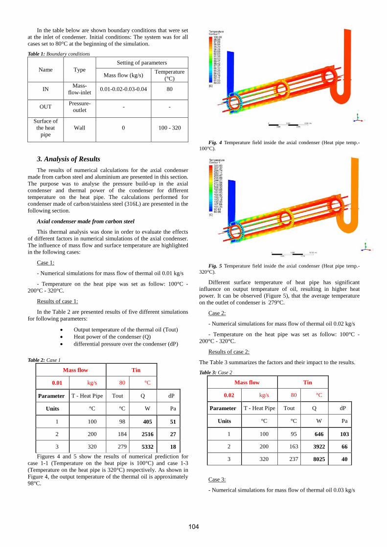
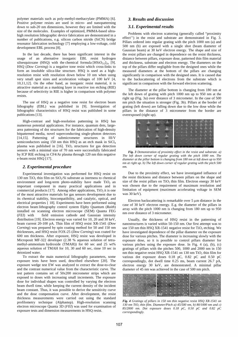
3 320 279 5332 18 Figures 4 and 5 show the results of numerical prediction for

case 1-1 (Temperature on the heat pipe is 100°C) and case 1-3 (Temperature on the heat pipe is 320°C) respectively. As shown in Figure 4, the output temperature of the thermal oil is approximately 98°C.

Fig. 4 Temperature field inside the axial condenser (Heat pipe temp.-100°C).

Fig. 5 Temperature field inside the axial condenser (Heat pipe temp.-320°C).

Different surface temperature of heat pipe has significant influence on output temperature of oil, resulting in higher heat power. It can be observed (Figure 5), that the average temperature on the outlet of condenser is 279°C.

Case 2:

- Numerical simulations for mass flow of thermal oil 0.02 kg/s

- Temperature on the heat pipe was set as follow: 100°C - 200°C - 320°C.

Results of case 2:

The Table 3 summarizes the factors and their impact to the results.

Table 3: Case 2

Mass flow Tin 0.02 kg/s 80 °C

Parameter T - Heat Pipe Tout Q dP

Units °C °C W Pa

1 100 95 646 103

2 200 163 3922 66

3 320 237 8025 40

Case 3:

- Numerical simulations for mass flow of thermal oil 0.03 kg/s

104

- Temperature on the heat pipe was set as follow: 100°C - 200°C - 320°C.

Results of case 3:

The Table 4 summarizes the factors and their impact to the results.

Table 4: Case 3

Mass flow Tin 0.03 kg/s 80 °C

Parameter T - Heat Pipe Tout Q dP

Units °C °C W Pa

1 100 92 791 158

2 200 149 4755 114

3 320 209 9594 81

Case 4:

- Numerical simulations for mass flow of thermal oil 0.04 kg/s

- Temperature on the heat pipe was set as follow: 100°C - 200°C - 320°C.

Results of case 4:

The Table 5 summarizes the factors and their impact to the results.

Table 5: Case 4

Mass flow Tin 0.04 kg/s 80 °C

Parameter T - Heat Pipe Tout Q dP

Units °C °C W Pa

1 100 90 888 90

2 200 138 5308 138

3 320 189 10635 189

Increasing the surface temperature on the heat pipe leads to the following result: the outlet temperature of the oil increases and consequently the heat power is higher and pressure drop is lower.

Summary - Axial condenser made from carbon steel

Figures 6 and 7 show dependence of the thermal power and the pressure difference of condenser for different flow.

Fig. 6 Thermal power of condenser for different Mass flow (MF).

Fig. 7 Differential pressure over the condenser for different Mass flow

(MF).

In Figure 6 is shown the impact of mass flow on thermal power. The power is higher by increasing flow to the condenser as well as the temperature on the heat pipe. The pressure drop decreases when surface temperature increases (Fig.7).

4. Conclusions The aim of this article was to evaluate the effect of different

factors to the parameters of the axial condenser. The influence of different mass flows and the temperatures on the heat pipe of condenser were investigated and following conclusions have been reached.

- The highest thermal power was observed in the case 4 (mass flow 0.04 kg/s and temperature on the heat pipe 320°C).

- The lowest differential pressure over the condenser was noticed in the case 1 (mass flow 0.01 kg/s and temperature on the heat pipe 320°C)

The thermal powers of the axial condenser reached a maximum value at the temperature 320 °C. By decreasing the temperature on the heat pipe the power of condenser was reduced. When the flow of thermal oil is rising, the condenser has better heat performance. This effect can be very well observed, when the temperature on the heat pipe is 320 °C and the flow rate is 0.04 kg/s.

In the pressure drop Fig. 7 can be observed that combination of high mass flow and high temperature causes low pressure drop. In regards to both thermal power and differential pressure, higher temperature and mass flow is better.

Acknowledgement This work is supported by the financial assistance of the

company Goodtech Recovery Technology AS.

This article is supported by the financial assistance of the project KEGA No. 042ŽU-4/2016 ”Chladenie na základe fyzikálnych a chemických procesov”.

References [1] LENHARD, R., MALCHO, M.: Numerical Simulation

Device for the Transport of Geothermal Heat with Forced Circulation of Media. Mathematical and Computer Modelling, vol. 57, No. 1-2, 111-125, 2013, ISSN 0895-7177.

[2] NEMEC P., CAJA A., MALCHO M.: Mathematical Model for Heat Transfer Limitations of Heat Pipe, Mathematical and Computer Modelling, 57, 1-2, 2013, 126-136.

[3] PILAT, P., PATSCH, M., MALCHO, M: Solar Heat Utilization for Adsorption Cooling Device, vol. 25, Article No. 01074, Conference on Experimental Fluid Mechanics, EFM 2011, Jicin, 2012.

[4] SCHMALHOFER, J., FAGHRI, A.: Heat Mass Transfer, 36, 201-212, 1993.

105

ELECTRON BEAM LITHOGRAPHY METHOD FOR HIGH-RESOLUTION NANOFABRICATION

RNDr. Kostic I.1, Prof. DSc. PhD. Vutova K.2, Ing. Bencurova A.1, Ing. Nemec P.1, Assoc. Prof. PhD. Koleva E.2

Institute of Informatics - Slovak Academy of Sciences, Bratislava, Slovakia 1 Institute of electronics - Bulgarian Academy of Sciences, Sofia, Bulgaria 2

ivan.kostic@savba.sk, katia@van-computers.com

Abstract: Electron beam lithography (EBL) is one of the few “top-down” methods and EBL is becoming increasingly widespread in R&D and small volume production due to its flexibility and mask-less nature, very high (sub-10 nm) resolution and accuracy and in many cases EBL is the only possible alternative. In this paper, obtained experimental and simulation results for EBL nano-patterning using the high-resolution electron beam resist Hydrogen Silsesquioxane (HSQ) are presented and discussed. The influence of EBL process parameters such as exposure dose, resist thickness and development process conditions on the obtained developed images is studied. The applied simulation tool for the resists’ characteristics evaluation is suitable for a precise control of obtained image dimensions in the resist applied as a masking layer for nano-patterning. This investigation and simulation of the characteristics of the studied e-beam resist aim to improve the resolution of the nano-dimensioned electron beam lithography and results for nano-lithography applications are also presented.

Keywords: ELECTRON BEAM LITHOGRAPHY, ELECTRON RESIST, EXPOSURE PROCESS, DEVELOPMENT PROCESS, EXPOSURE DOSE, RESIST PROFILES, RESOLUTION, MONTE CARLO SIMULATION, PROXIMITY EFFECT

1. Introduction There are two main nanofabrication approaches: (i) bottom-up

approach – the structures and devices are created from small to large, i.e. assembled from their subcomponents (atoms, molecules or even cells) in an additive fashion; and (ii) top-down approach – the fabrication goes from large to small using sculpting or etching to carve nanostructures and devices from a larger piece of material in a subtractive fashion.

The polymer based electron beam lithography (EBL) is one of the most widely applied techniques for the production of nanostructures in R&D, for prototyping, production of photomask and imprint mold. Application range is wide, i.e. the development of sensors, nanophotonic devices, high frequency electronics, spintronics, molecular electronics, Bit-patterned media, quantum dots, nanowires, nanomechanical devices, etc.

Various limitations of EBL resolution - spot size, electron scattering, secondary-electron range, resist development, and mechanical stability of the resist are subject of research in the attempt to push further the boundaries of EBL down into the nanometer range.

EBL allows the direct writing of nanostructures with dimensions below 100 nm and in special cases even with sub-10 nm dimensions. Achieving sub-100 nm structures using EBL is a very sensitive process determined by various factors, starting with the choice of polymer resist material and ending with the development process.

Resist materials are crucial elements in EBL and their performance determines the final results of the structures patterning. Our aim in this paper is to characterize electron sensitive material – a high-resolution negative electron beam resist Hydrogen Silsesquioxane (HSQ). Experimental and simulation results obtained for EBL nano-patterning using this resist are presented and discussed.

1.1. Electron beam lithography method

Electron beam lithography is based on physico-chemical changes in the resist thin layer [1]. The commonly used resists are polymers dissolved in a liquid solvent with small molecule additives to enhance the lithographic performance of the material.

During the electron beam exposure, the result of inelastic collisions of electrons with the resist is the ionization (secondary electron generation), where an incoming electron provides enough energy to cause an electron to be removed from an atom. In polymers, these lead to many different chemical reactions, which are classified as either chain-scission or crosslinking reactions.

In case of chain-scission, a polymer chain is broken up into much smaller pieces. This reduces the molecular weight of the resist, which makes it more soluble in an organic solvent (developer). The exposed area is dissolved away, leaving unexposed areas of the resist to form the designed pattern. In this case, polymer is used as a positive resist. If crosslinking polymers form three-dimensional structures during an electron beam exposure, then the exposed areas are insoluble in a solvent. In such case polymers are used as a negative resist. Typical positive and negative resist profiles are shown in Fig. 1 [2].

Fig. 1 Resist profile of 600 nm thin positive resist CSAR62 on silicon

substrate (a), and 600 nm thin negative resist SU-8 on silicon substrate (b).

The lithography process consists of the following technological steps: surface preparation (cleaning, dehydration, adhesion promoter application), resist coating (spin coating, spray coating, pre-bake (soft bake), exposure, post-exposure bake (PEB), development, post-bake (hard bake), processing the resist as a masking film, resist stripping, post process cleaning (ashing) [3].

General scheme of the resist based electron beam lithography process is shown in Fig. 2. The electron energy can be varied from 1 keV up to 100 keV, however, for high-resolution patterning is convenient 30, 50 and 100 keV, depending on the equipment complexity.

Fig. 2 General scheme of the lithography process [2].

The resolution of electron beam lithography is set by various factors such as beam size, resist material, exposure dose, development process and also the writing strategy [4].

1.2. Materials sensitive to electron irradiation The resolution of electron optical systems can approach 0.1 nm,

so the ultimate resolution of electron beam lithography is set by the resolution of the resist and by the subsequent fabrication process [5], therefore superior resists are crucial for the application of e-beam lithography. Commonly used electron beam resists are

106

polymer materials such as poly-methyl-methacrylate (PMMA) [6]. Positive polymer resists are used in micro- and nanopatterning down to sub-20 nm dimensions, however they are limited with the size of the molecules. Examples of optimized, PMMA-based ultra-high resolution lithographic device fabrication are demonstrated in a number of publications, e.g. silicon carbon nitride (SiCN) bridge resonator fabrication technology [7] employing a low-voltage, cold development EBL process [8].

In the last decade, there has been significant interest in the usage of an alternative inorganic EBL resist hydrogen silsesquioxane (HSQ) with the chemical formula [HSiO3/2]2n [9]. HSQ (Dow Corning) is a negative tone resist which cross-links to form an insoluble silica-like structure. HSQ is used as a high-resolution resist with resolution down below 10 nm when using very small spot sizes and acceleration voltages of 100 keV [4, 10,11,12]. On the other hand, as inorganic resist material, it is attractive material as a masking layer in reactive ion etching (RIE) because of selectivity in RIE is higher in comparison with polymer resists.

The use of HSQ as a negative tone resist for electron beam lithography (EBL) was published in [9]. Investigation of lithographic characteristics of HSQ resist was published in some publications [13].

High-contrast and high-resolution patterning in HSQ has numerous potential applications. For instance, quantum dots, large-area patterning of dot structures for the fabrication of high-density bitpatterned media, novel superconducting single-photon detectors [14,15]. Patterning of submicrometer structures in III/V semiconductors using 150 nm thin HSQ as an etch mask in SiCl4 plasma was published in [16]. TiO2 structures for gas detection sensors with a minimal size of 70 nm were successfully fabricated by ICP RIE etching in CF4/Ar plasma through 120 nm thin negative e-beam resist HSQ [17].

2. Experimental procedure Experimental investigation was performed for HSQ resist on

130 nm TiO2 thin film on SiO2/Si substrate as inertness to chemical environment and long-term photo-stability have made TiO2 an important component in many practical applications and in commercial products [17]. Among other applications, TiO2 it is one of the most attractive materials for gas sensors development due to its chemical stability, biocompatibility, and catalytic, optical, and electrical properties [ 18]. Experiments have been performed using electron beam lithography control system Elphy Quantum (Raith) installed on scanning electron microscope (SEM) Quanta FEG (FEI) with field emission cathode and Gaussian intensity distribution [19]. Electron energy was varied for 10, 20 and 30 keV, beam current 20-100 pA. Thin film of HSQ resist XR-1541 (Dow Corning) was prepared by spin coating method for 50 and 150 nm thicknesses, and HSQ resist FOX-25 (Dow Corning) was coated for 600 nm thickness. After exposure, HSQ resist was developed in Microposit MF-322 developer (2.38 % aqueous solution of tetra-methyl-ammonium hydroxide (TMAH)) for 60 sec and 25 wt% aqueous solution of TMAH for 10, 30 and 60 sec, rinse 10 sec in deionized water.

To extract the main numerical lithography parameters, some exposure tests have been used, described elsewhere [20]. The exposure wedge test EW was analyzed to extract the dose-to-clear and the contrast numerical value from the characteristic curve. The test pattern contains set of 50x200 micrometer strips which are exposed to doses with increasing small increments. The exposure dose for individual shapes was controlled by varying the electron beam dwell time, while keeping the current density of the incident beam constant. Thus, it was possible to derive the sensitivity curve and the dose compensation curve. After development, the resist thickness measurements were carried out using the standard profilometry technique (Alphastep). High-resolution scanning electron microscope Quanta 3D (FEI) was used for examination of exposure tests and dimension measurements in HSQ resist.

3. Results and discussion

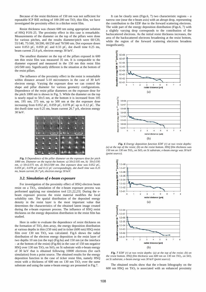
3.1. Experimental results Problems with electron scattering (generally called “proximity

effect’’) in the resist and substrate are demonstrated in Fig. 3. Pillars ordered into regular grating with the pitch 1000 nm (a) and 500 nm (b) are exposed with a single shot (beam diameter of Gaussian beam) at 30 keV electron energy. The shape and size of the resist pillars are changed in dependence on the resist thickness, distance between pillars, exposure dose, patterned thin film material and thickness, substrate and electron energy. The diameters on the top of the pillars differ negligible from the designed ones while the measured diameters at the bottom of the pillars are changing significantly in comparison with the designed ones. It is caused due to the backscattering of electrons from the substrate which is significant in comparison with the forward electron scattering.

The diameter at the pillar bottom is changing from 180 nm at the left down of grating with pitch 1000 nm up to 950 nm at the right up (Fig. 3a) over distance of 3 micrometer. In the case of 500 nm pitch the situation is stronger (Fig. 3b). Pillars at the border of grating (left down) are falling down due to the low dose while the pillars in the distance of 3 micrometer from the border are overexposed (right up).

Fig. 3 Demonstration of proximity effect in the resist and substrate. a)

The left down corner of regular grating with the pitch 1000 nm. The diameter at the pillar bottom is changing from 180 nm at left down up to 950 nm at right up. b) The left down corner of regular grating with the pitch 500 nm.

Due to the proximity effect, we have investigated influence of the resist thickness and distance between pillars on the shape and size of the resist pillars on TiO2 thin film. Electron energy 30 keV was chosen due to the requirement of maximum resolution and limitation of equipment (maximum accelerating voltage in SEM was 30 keV).

Electron backscattering is remarkable over 5 µm distance in the case of 30 keV electron energy. E.g. the diameter of the pillars in array with the pitch 1000 nm is changing from 180 nm up to 950 nm over distance of 3 micrometer.

Usually, the thickness of HSQ resist in the patterning of nanostructures is varied within 50-150 nm. Our first attempt was to use 150 nm thin HSQ XR-1541 negative resist for TiO2 etching. We have investigated dependence of the pillar diameter on the exposure dose for various pitches. The diameter is increasing slowly with the exposure dose, so it is possible to control pillars diameter for various pitches using the exposure dose. In Fig. 4 (a), (b), (c) gratings of pillars with the pitches 500, 1000 and 2000 nm in 150 nm thin negative resist HSQ XR-1541 on 130 nm TiO2 thin film for various dot exposure doses 0.18 pC, 0.82 pC and 0.50 pC correspondingly, dot dwell time 0.25 ms, beam current 26.7 pA, electron energy 30 keV, are demonstrated. A minimal pillar diameter of 45 nm was achieved in the case of 500 nm pitch.

Fig. 4 Gratings of pillars in 150 nm thin negative resist HSQ XR-1541 on 130 nm TiO2 thin film. Diameter/Pitch a) 45/500 nm, b) 80/1000 nm and c) 85/2000 nm. Dot exposure doses 0.18 pC, 0.50 pC and 0.82 pC correspondingly.

107

Because of the resist thickness of 150 nm was not sufficient for repeatable ICP RIE etching of 100-200 nm TiO2 thin film, we have investigated the proximity effect in a thicker resist film.

Resist thickness was chosen 600 nm using appropriate solution of HSQ FOX-25. The proximity effect in this case is remarkable. Measurements of the diameter on the top of the pillars were done for various pitches, and the results diameter/pitch were 60/120, 55/140, 75/160, 50/200, 60/250 and 70/500 nm. Dot exposure doses were 0.053 pC, 0.059 pC and 0.33 pC, dot dwell time 0.25 ms, beam current 25.6 pA, electron energy 30 keV.

The smallest diameter on the top of the pillars exposed in 600 nm thin resist film was measured 35 nm. It is comparable to the diameter exposed and measured in the 150 nm thin resist film (45/500 nm). Significantly different is the situation at the bottom of the resist pillars.

The influence of the proximity effect in the resist is remarkable within distance around 5-10 micrometers in the case of 30 keV electron energy. Varying the exposure dose we can control the shape and pillar diameter for various geometry configurations. Dependence of the resist pillar diameters on the exposure dose for the pitch 1000 nm is shown in Fig. 5. While the diameter on the top is nearly equal to 50±5 nm, at the bottom it is increased from 105 nm, 195 nm, 375 nm, up to 500 nm at the dot exposure dose increasing from 0.052 pC, 0.059 pC, 0.078 pC up to 0.12 pC. The dot dwell time was 0.25 ms, beam current 26.7 pA, electron energy 30 keV.

Fig. 5 Dependence of the pillar diameter on the exposure dose for pitch

1000 nm. Diameter on the top/at the bottom: a) 50±5/105 nm, b) 50±5/195 nm, c) 50±5/375 nm, d) 50±5/500 nm. Dot exposure dose was 0.052 pC, 0.059 pC, 0.078 pC and 0.12 pC correspondingly, dot dwell time was 0.25 ms, beam current 26.7 pA, electron energy 30 keV.

3.2. Simulation of e-beam exposure For investigation of the proximity effect of HSQ electron beam

resist on a TiO2, simulation of the e-beam exposure process was performed applying our simulation tool [21,22,23]. During the e-beam exposure process the resist material modifies the local solubility rate. The spatial distribution of the deposited energy density in the resist layer is the most important value that determines the characteristics of the obtained latent image created during the e-beam exposure process. The influence of HSQ resist thickness on the energy deposition distribution in the resist film has studied.

Here in order to evaluate the dependence of resist thickness on the formation of TiO2 dots array, the energy deposition distribution at various depths in thin (150 nm) and in ticker (600 nm) HSQ resist film over 130 nm TiO2 was calculated. Fig.6 shows the radial distribution of the electron energy deposition in the resist layer of two depths 10 nm (on the top) (Fig.6a) and 150 nm (at the interface – at the bottom of the resist) (Fig.6b) in the case of 150 nm negative HSQ over 130 nm TiO2 on SiO2 on Si substrate with e-beam energy of 30 keV that is obtained following 10000 electrons (for each simulation) from a point source. The obtained results for the energy deposition function in the case of ticker resist film, namely HSQ resist with a thickness of 600 nm on 130 nm TiO2 over the same substrate and using the same e-beam energy are presented in Fig.7.

It can be clearly seen (Figs.6, 7) two characteristic regions – a narrow one (near the e-beam axis) with an abrupt drop, representing the contribution to the EDF due to the forward scattering electrons. The wide part of the energy deposition distribution (Figs.6, 7) with a slightly varying drop corresponds to the contribution of the backscattered electrons. As the initial resist thickness increases, the area of the backscattered electrons broadening at the resist bottom, while the region of the forward scattering electrons broadens insignificantly.

(a)

(b)

Fig. 6 Energy deposition function EDF (r) at two resist depths: (a) at the top of the resist; (b) on the resist bottom. HSQ film thickness was 150 nm on 130 nm TiO2, on SiO2 on Si substrate, e-beam energy was 30 keV (point source).

(a)

(b)

Fig. 7 EDF (r) at two resist depths: (a) at the top of the resist; (b) on the resist bottom. HSQ film thickness was 600 nm on 130 nm TiO2, on SiO2 on Si substrate, e-beam energy was 30 keV (point source).

The obtained results show that the e-beam lithography on the 600 nm HSQ on TiO2 is associated with an enhanced proximity

108

effect in comparison with that on the 150 nm HSQ on TiO2 and especially at the bottom of the resist (Fig.7b). The ticker HSQ resist film causes an additional backscattering of penetrating electrons and, hence, an additional proximity effect in comparison with the thinner resist layer. This effect is greater in the ticker HSQ resist film and especially at the bottom of the resist as it is also demonstrated in the experimental results (Figs.4, 5). Therefore, the HSQ resist film is used must be thin as possible for fine TiO2 dots array formation.

4. Conclusions Experimental and simulation results for EBL nano-patterning

using the high-resolution electron beam resist Hydrogen Silsesquioxane (HSQ) on TiO2 thin film at 30 keV electron energy were presented and discussed. Dependence of pillar diameters on the exposure dose for 600 nm thin HSQ resist was studied. The influence of the HSQ resist thickness and the distance between the pillars on the shape and size of the HSQ resist pillars on TiO2 thin film was studied. A minimal diameter of 50/105 nm on the pillar top/at the pillar bottom in the case of 600 nm thin HSQ resist was achieved. A minimal pillar diameter was 45 nm in the case of 150 nm thin HSQ resist on TiO2 thin film.

Using our Monte Carlo simulation tool we calculated energy deposition distributions in the samples of 150-nm-thick and 600-nm-thick HSQ resist layers on 130 nm TiO2 in order to evaluate the proximity effect on the resist thickness for the formation of fine dot arrays using e-beam energy of 30 keV. It is necessary to use the thinner resist film for patterning of dots array in TiO2 films.

Acknowledgements This work was supported by the Bulgarian National Fund for Scientific Research under contract DNTS/Slovakia 01/1/2016 (project NTS/Slovakia 01/25-13), the project APVV SK-BG-2013/0030, and by the Ministry of Education of the Slovak Republic and the Slovak Academy of Sciences under the Contract VEGA 1/0828/16. SEM facilities at the Institute of Electrical Engineering SAS are gratefully acknowledged. The joint research project SAS-BAS 2015-2017 is acknowledged.

References [1] McCord M.A., M.J. Rooks. Handbook of Microlithography,

Micromachining and Microfabrication. 1st ed., edited by P. Rai-Choudhury (IEE, London). I (Chap. 2), 1997, pp. 139–249.

[2] Saburo N., U. Takumi, and I. Toshio. Microlithography Fundamentals in Semiconductor Devices and Fabrication Technology. New York: Marcel Dekker, 1998.

[3] Kostic, I., K. Vutova, E. Koleva, R. Andok, A. Bencurova, A. Konecnikova, G. Mladenov. Study on polymers with implementation in electron beam lithography. Polymer Science: Research advances, practical applications and educational aspects. Spain: Formatex Research Center, polymer Science Book Serie No. 1, 2016, pp. 488-497.

[4] Grigorescu A. E., M. C. van der Krogt and C. W. Hagen. Limiting factors for electron beam lithography when using ultra-thin hydrogen silsesquioxane layers. J. Micro/Nano- lithogr. MEMS, MOEMS, 6, 2007, p. 043006.

[5] Broers A.N., A.C.F. Hoole, J.M. Ryan. Electron beam lithography—Resolution limits. Microelectronic Engineering, 32, 1996, p. 131.

[6] Hatzakis M. Electron resists for microcircuit and mask production. J. Electrochem. Soc., 116, 1969, pp. 1033-37.

[7] Fischer L.M., L.M.N. Wilding, M. Gel, S. Evoy. Low-stress silicon carbonitride for the machining of high-frequency nanomechanical resonators. Journal of Vacuum Science and Technology B, 25, 2007, p. 33.

[8] Mohammad M.A., C. Guthy, S. Evoy, S.K. Dew, M. Stepanova. Nanomachining and Clamping Point Optimization of Silicon Carbon Nitride Resonators using Low Voltage

Electron Beam Lithography and Cold Development. Journal of Vacuum Science and Technology B, 28, 2010, p. C6P36.

[9] David B. Cordes, P. D. Lickiss, F. Rataboul. Recent Developments in the Chemistry of Cubic Polyhedral Oligosilsesquioxanes. Chem. Rev., 110 (3), 2010, pp. 2081–2173.

[10] Grigorescu A.E., C.W. Hagen. Resists for sub-20-nm electron beam lithography with a focus on HSQ: state of the art. Nanotechnology, 20, 2009, p. 292001.

[11] Yamazaki K., H. Namatsu. 5 nm-order electron-beam lithography for nanodevice fabrication. Japan. J. Appl. Phys., 43, 2004, p. 3767.

[12] Maile B. E.,W. Henschel, H.Kurz, B. Rienks, R. Polman and P. Kaars. Sub-10nm linewidth and overlay performance achieved with a fine-tuned EBPG-5000TFE electron beam lithography system. Japan. J. Appl. Phys., 39, 2000, p. 6836.

[13] Kostic I., A. Bencurova, A. Konecnikova, P. Nemec, A. Ritomsky, E. Koleva, K. Vutova, G. Mladenov. Study of electron beam resists: negative tone HSQ and positive tone SML300. Elektrotechnika I elektronika E+E, 49 (5-6), 2014, pp. 279-283.

[14] Yang J. K. W., E. Dauler, A. Ferri, A. Pearlman, A. Verevkin, G. Gol’tsman, B. Voronov, R. Sobolewski, W. E. Keicher, and K. K. Berggren. Fabrication development for nanowire GHz-counting-rate single-photon detectors. IEEE Trans. Appl. Supercond., 15, 2005, p. 626.

[15] Rosfjord K. M., J. K. W. Yang, E. A. Dauler, A. J. Kerman, V. Anant, B. M. Voronov, G. N. Gol’tsman, and K. K. Berggren. Nanowire single photon detector with an integrated optical cavity and anti-reflection coating. Opt. Express, 14, 2006, p. 527.

[16] Kostic I., R. Andok, A. Bencurova, N. Glezos, S. Hascik, A. Konecnikova, P. Nemec, A. Ritomsky, J. Skriniarova. Investigation of e-beam resists for structure patterning in the nanophotonic device fabrication. Proceedings of ADEPT : 2nd Intern. Conf. on Advances in Electronic and Photonic Technologies. Eds. Pudiš, D. et al., University of Žilina, Taranska Lomnica, Slovakia, June 1.-4. 2014, pp. 241-246.

[17] Kamat P. V. TiO2 nanostructures: recent physical chemistry advances. J. Phys. Chem. C, 116, 2012, pp. 11849–51.

[18] Hotovy I., I. Kostic, P. Nemec, M. Predonacy, V. Rehacek. Patterning of titanium oxide nanostructures by electron-beam lithography combined with plasma etching. .Journal of Micromechanics and Microengineering, 25 (7), 2015, p. 074006.

[19] https://www.raith.com [20] Andok R., L. Matay, I. Kostic, A. Bencurova, P. Nemec, A.

Konecnikova, A. Ritomsky. Estimation of exposure parameters of chosen e-beam resists using variable shaped e-beam pattern generator. Proc. ASDAM 2012, 9th Int. Conf. on Advanced Semiconductor Devices and Microsystems, Smolenice Nov 11-15. Piscataway: IEEE, 2012, pp. 287-290.

[21] Vutova, K., G. Mladenov, I. Raptis, A. Olziersky. Process simulation at electron beam lithography on different substrates. Journal of Materials Processing Technology, 184 (1-3), 2007, pp. 305-311.

[22] Vutova K., G. Mladenov. Chapter 17. Computer simulation of Processes at Electron and Ion Beam Lithography, Part 1: Exposure modeling at electron and ion beam lithography, in: M. Wang, ed., Book Lithography, INTEH, 2010, pp. 319-350.

[23] Mladenov G., E. Koleva, K. Vutova. Electron lithography of submicron and nano structures. Chapter in a special review book “Practical Aspects and Applications of Electron Beam Irradiation”, еds.: M.Nemtanu, M.Brasoveanu, publ. Research Signpost/ Transworld Research Network, 2011, pp. 135-166.

109

A METHOD OF HEAT TREATMENT CONTROL THROUGH EDDY CURRENT TESTING AND DOE

МЕТОД ЗА КОНТРОЛ НА ТЕРМИЧНАТА ОБРАБОТКА ЧРЕЗ ИЗСЛЕДВАНЕ С ВИХРОВИ ТОКОВЕ И ПЛАНИАРАН ЕКСПЕРИМЕНТ

Ivanov J.St., MSc

“M+S Hydraulic”AD, Kazanlak, Bulgaria jeanivanov@yahoo.de

Abstract: A designed experiment was conducted, which was aimed at studying two technological factors of 20CrMo5 steel low-temperature tempering, namely temperature and duration. The quality indices which were measured are Vickers hardness /HV50/ and the eddy current characteristic /Z/. The experiment identified and analyzed the adequacy of regression models of the two quality indices. A method is presented for a joint analysis of the two regression models with the purpose of using the results in heat treatment control. The study confirmed the joint effect of the two technological factors, the temperature and time of low-temperature tempering, as well as the sensitivity of the eddy currents study to their variation.

KEY WORDS: DESIGNED EXPERIMENT, TECHNOLOGICAL FACTORS, VICKERS HARDNESS, EDDY CURRENTS, REGRESSION MODEL

1. Introduction The final stage of every thermochemical treatment which

consists of carburizing and quenching is low-temperature tempering (LTT). It is conducted at temperatures between 100 и 250°С and helps reduce the risk of cracks and inner stress [1]. In most cases control is focused on the properties of the quenched diffusion layer. Its microstructure is studied, as well as existing layer defects, such as a high content of residual austenite or the presence of carbides; the hardness is measured through different methods; and the effective layer depth is determined /with the characteristic hardness of 550 HV1/.

The investigation of carburized steel core is limited to hardness measurements, and metallographic tests are done to locate the presence of non-quenched phases – ferrite [15]. The properties of the base steel core are not connected with carbon diffusion. They are largely determined by the metallurgical production of steel and they are very important for the reliable long-lasting performance of parts. Within the same grade, the different melts may have alloying elements and a microstructure, which may result in significant differences in the properties after quenching – hardenability, hardness penetration, grain size, etc. Sometimes the hardenability test performed in the metallurgical plant gives a fair idea about the expected properties. However, when the final quenching is preceded by a normalization, first quenching and high-temperature tempering or pearlite-ferrite structure annealing, then the hardenability test data only has reference value, which is mainly due to the grain refinement and the changes that have occurred in the phase contents and the phase dispersity. Furthermore, the core hardness strongly affects the HV- hardness variation pattern when the effective depth is being measured. Due to the computer-controlled gas carburizing, in determining the thermochemical processing modes, it is necessary to introduce corrections connected with the alloying content, the so-called alloying factor- f. Depending on the type of steel and when the process uses uncontrolled combinations of parts of the same steel grade, but different melts, producers, etc., it is possible to end up with a batch of parts with various core properties after the thermochemical treatment, and very similar surface properties, i.e. properties of the diffusion layer. For example, the characteristic hardness values of 20 CrMo5 steels are within 58-60 HRC. The hardness values of the core, however, can vary within 10 units HRC. Apparently, the metallurgical properties of steel alone can, even with a stable process of thermochemical treatment, significantly affect the operational qualities. Here is the other distinguishing feature of core properties. The core obtains its final properties after a thermal treatment while only rarely do surface layers go without additional mechanical processing or shot peening /strengthening/. There are also parts with zones where the presence of carburized and quenched layer is not desirable, because of developing flaws and

surface tensile stress. Usually, such zones, for instance, ones with threads, are either protected from carburizing, or before the final quenching they have the carburized layer removed from them.

The control plans of the different parts after thermochemical treatment, only very rarely, include hardness, microstructure and the granulometric composition of the core. All requirements mostly concern the surface quality indices. Naturally, in order to determine the core properties, it is necessary to break a part or a witness of the heat treatment which was made from the same steel. Even then, with a random approach and a lack of batch organization, or when steel of different melts is used, it will not be possible for the quality control check results to spread to all parts of the same batch. If consistency is applied to each melt of steel until it is all used, it will certainly lead to a reduction in the core properties dispersion[5]. An even better approach would be if all orders and deliveries could be for steels of the necessary grades with a very narrow hardenability range. This would mainly lead to a stabilization of the operational qualities, which in itself is a prerequisite of good quality.

However, there remains the question of how to study the core properties and how to evaluate their effect on the performance of parts after thermochemical processing. The steels designated for carburizing are rarely used after quenching and annealing alone. That is the reason why data of their post-annealing properties, except for high-temperature annealing, is usually non-existent. The introduction of non-destructive methods of control, e.g. through eddy currents, together with other ones for the determination of various mechanical properties allows for an easy and plausible study of big groups of parts [6, 7, 8, 9]. The determination of statistical dependences is a major task, which can be done through designed experiments and regression analyses [11, 12]. The sensitivity of the eddy current study to the variation of the LTT technological factors – temperature and duration – has been repeatedly established [13, 14], but mostly for carburized surfaces. Rarely, if ever, is there data of variations in carburized and quenched steels with zones of removed carburization, i.e. on the surface of the base steel. Design and technical documentations, as well as specialized technical literature often feature levels of the technological factors: temperature and duration of low-temperature tempering, without taking into consideration the specific nature of parts and the depth of developing structural changes. Recommended temperatures are in the range of 160-180°С, minimum 1,5 h [10]. The same author published data of mechanical properties in the 100-200°С range and put emphasis on the major effect which the LTT mode has on the yield strength. Other authors have described studies of the mechanical properties after tempering at 180°С for 4 h [2]. With tempering at over 150°С, mostly at 180°С the studies registered a 1-5 HRC [4] reduction in the hardness on the surface of carburized parts.

110

The analyzed studies were prompted by the obvious production need for gradual and consistent increase in quality, and by cases of premature destruction of parts put through thermochemical processing, which included gas carburizing, quenching and LTT. A series of observations suggested several possible reasons:

1. Inadequate LTT. 2. Possible development of hydrogen embrittlement [3]. 3. High tensile stress on the surface caused by design,

technological and structural factors. As we all know, these are interconnected, and LTT in air brings about structural changes, and also a reduction in stresses and hydrogen evacuation. Both diffusion processes, i.e. those of hydrogen and carbon, and all such processes, are affected both by temperature and time. Surely, time durations of less than 2 h can hardly lead to a completion in the occurring changes?

2. Object of research Samples of 20CrMo5 steel, WN 1.7264 have been made for

tensile strength testing and hardness measurements.

Steel is the main material for hydraulic motors shafts with a conical outgoing part, and it has the following chemical composition, Table 1.

Таble 1. Chemical composition of 20CrMo5 steel

%С %Si %Mn %P %S %Cr %Mo Min. 0.18 0.15 0.90 1.10 0.20 Max. 0.23 0.35 1.20 0.035 0.035 1.40 0.30

Table 2 presents data of tensile strength and hardness at different temperatures of LTT.

Таble 2. Hardness and tensile strength of 20CrMo5 after quenching and LTT ( Technical Card Gruppo Lucefin ) .

HB 353 353 319 HRC 38 38 34 Rm [N/mm2] 1180 1180 1050 Т temp. [°С] 100 200 300

The shafts end in a thread, which is the zone of concentration of all kinds of flaws of carburized and quenched layers. That is why a technological solution is found in the carburized layer removal before the final quenching.

3.Objectives of research The studies represent a stage in the search of the optimal mode

of LTT - temperature and time.

Eddy current testing could be used to determine zones of 100% acceptance control of LTT of conical threaded shafts with a maximum, medium and minimum hardness of the core in the range of 170 - 250°С and duration of 1 - 7 h. The eddy current testing results shall be used to introduce statistical control in the thermochemical processing.

4. Methodology of research

A complete factor experiment has been conducted with the following levels of technological factors [11]:

- Quenching temperature: 830 °С and 870 °С; - Тempering temperature-Tan.: 170 °С, 210 °С and 250°С; - Tempering time-TAUan : 1, 4 and 7 h.

Vickers hardness has been measured - HV50, BDS EN ISO 6507-1 [16], as well as the eddy current characteristic – Z [7]. Mean values were used after a normality test /normal distribution test/. The data was processed by means of regression analysis [12]. The eddy currents variation was analysed as a quality index [13]. The resulting regression models were presented graphically and

analysed for their adequacy. The joint examination of the contour diagrams of the two models in the field of variation of the technological factors, tempering temperature and time, offers an opportunity to calibrate the eddy current tests with relation to the desired hardness.

5.Test results

This paper presents the experimental findings of samples, quenched at 870°С. The mean values of hardness, HV50, and the eddy current characteristic Z are presented in Table 3, with coded levels of the technological factors. Тable 3. Results of measuring hardness and the eddy current characteristic.

Test № Tan. TAUan HV50 Z 1 -1 -1 440 3.40 2 -1 0 442 4.60 3 -1 1 423 4 4 0 -1 434 3.80 5 0 0 436 4.60 6 0 1 436 5 7 1 -1 397 3.40 8 1 0 412 5.50 9 1 1 413 5.60

5.1. Regression model for hardness HV50 The following regression model has been established - REG-HV50:

(1) y = 439.645-13.871x1-14.627x1x1+7.950x1x2-5.930x2x2 where:

x1 <--> Tan x2 <--> TAUan y <--> HV50.

The regression equation takes into account the significant primary effect of the tempering temperature on hardness, as well as the weaker effect of the tempering time factor, which follows in importance the effect of the joint influence of the two factors.

5.2. Regression model for the eddy current characteristic The eddy current testing resulted in the following model: REG-Z:

(2) y = 4.900+0.417x1+0.667x2-0.700x2x2+0.400x1x2 where:

x1 <--> Tan x2 <--> TAUan y <--> Z . The eddy current characteristic is affected by both technological

factors, the prevailing one being the tempering time. This regression model REG-Z also takes into account the joint influence of the two technological factors.

The statistical analysis of the regression models proves that they are adequate - Таble 4.

Таble 4. Adequacy indices of models REG-HV50 and REG-Z.

REG-HV50 REG- Z R-sq= 0,9848 0,9515 Radj-sq= 0,9697 0,903 R-sq(pred)= 0,9254 0,7642 F 64,99 19,61 P 0,00068 0,00683

The contour diagrams and 3D surface graphs for the two models are presented in Fig. 1; 2; 3; 4. The maximum values in the technological factors variation field are also given.

111

REG-HV50 REG- Z

Maximum value: 444 HV50

x1 = -0,58 x2 = -0,39

Мinimum value: 397 HV50 x1 = 1 x2 = -1

Maximum value: 5,72 x1 = 0,99 x2 = 0,76

Мinimum value: 3,52 x1 = -1 x2 = -1

Fig.1. Constant values contours for model REG-HV50.

Fig.2. Constant values contours for model REG- Z.

-1.00

-0.50

0.00

0.50

1.00-1.00

-0.500.00

0.50

1.00

400

410

420

430

440

-1.00

-0.50

0.000.50

1.00

-1.00-0.50

0.000.50

1.00

4.00

4.50

5.00

5.50

Fig.3. 3D surface graph for

model REG-HV50. Fig.4. 3D surface graph for

model REG- Z.

The joint presentation of the two models through constant values contours is shown in Fig.5.

Fig.5. Constant values contours for the eddy current characteristic in

the hardness variation field HV50.

Three characteristic zones can be distinguished in the hardness variation field:

- Maximum hardness zone - HV50 >440; - Minimum hardness zone - HV50 <412; - Zone of very smooth variation of hardness - HV50 436-

438.

Fig.6. Values of the eddy current characteristic Z in the zone of maximum hardness above 440 HV50.

With the introduced limits of hardness, these zones are illustrated graphically in Fig. 6; 7; 8. Fig 6 shows the variation of the eddy current characteristic in the zone of maximum hardness. The zone is limited with tempering temperatures of up to around 204°С and time of up to around 5 h.

The zone of smooth variation of hardness is located close to tempering temperatures of around 180 - 218 °С and tempering time above 4,5 h. The zone is homogeneous as regards the expected hardness after LTT.

Fig.7. Values of the eddy current characteristic Z in the zone of smooth

variation of hardness 436-438 HV50.

The minimum hardness values are located close to the maximum studied temperature, 250°С, and the minimum tempering time, Fig.8. The eddy currents characteristic has almost the same variation range as the one with the maximum hardness, but the values are valid for technological temperatures above 240 °С.

Fig.8. Values of the eddy current characteristic Z in the zone of

minimum hardness below 412 HV50.

Technologically, with tempering temperatures: 180 +/-5 °С, 210 +/-10 °С and 245 +/- 5 °С and tempering times of 1 tо 7 h, the following graphs can be shown: Fig.9; 10 and 11. These present the respective sections of the area illustrated in the diagram in Fig.5.

Fig.9. Hardness and the Eddy current characteristic in the technological zone of factors Тan=180 +/-5 °С.

Fig.10. Hardness and the Eddy current characteristic in the technological zone of factors Тan=200 +/-10 °С.

112

Fig.11. Hardness and the Eddy current characteristic in the

technological zone of factors Тan=245 +/-5 °С.

Each one of the presented diagrams could be viewed as a map of the respective final technological stage. The technological time control is beyond doubt. Achieving uniformity can be difficult because of the influence of the quantities of parts loaded for tempering, the specifics of furnaces, the vertical arrangement of parts and their proximity to the furnace door. That is why even when temperature adjustments are accurate and smooth, this does not guarantee one and the same effect on the properties of different parts.

6. Discussion The simultaneous analysis of outcomes for the two quality

indices HV50 and Z can be complemented with data of yield strength, tensile strength, and a number of other mechanical and even performance qualities. The enrichment of data with new results from 20CrMo5 steel samples, from different melts, with different hardenability, can be valuable information data base for a justified choice of a technological mode of low-temperature tempering. The two regression models have a different structure and take into account different effects of technological factors. The established statistical dependences can be used for establishing functional correlations. The analysis of the eddy current characteristic as a quality index, which is a controlled, non-destructive value is supported by its integral nature. This is determined by the essence of the eddy current testing, connected with the currents penetrating deep in the part, in accordance with the chosen operating frequency. Thus, besides the surface properties, there are also structural modifications, connected with the diffusion processes of low-temperature tempering; changes are registered in the state of stress and the electro-magnetic characteristics of the newly formed carbide phase.

The presented sequence of a designed experiment and regression models, which connect some quality indices with the starting levels of the technological factors, can be summarized not only as a method of research, but also as a method of non-destructive control of the outcome of technological activity. The stages in this method are as follows:

1. Planning and conducting the experiment. 2. Regression analysis of the findings on quality indices,

including the eddy current testing. 3. Regressions adequacy test. 4. Joint analysis of two or more regression models in their

information-technological and control aspect 5. Choice of a cost-effective technological mode of low-

temperature tempering and drawing up a control plan.

For the sake of brevity the method can be called „R+RZ”, as it represents a joint examination of a quality index regression and an eddy current characteristic regression. The method in the present case is applicable to the control of parts which have their carburized layer removed in certain sections after they have been put through carburization, quenching and LTT.

7. Conclusion Studying the effects of LTT on a particular steel grade or parts,

especially in mass production, is becoming increasingly important. The traditionally tested microstructure, hardness and other mechanical properties do not allow for the introduction of statistical methods of control. The eddy current testing is especially sensitive to the final stage in every carburizing and quenching process, i.e. LTT. Its speed can make it possible to cover a complete group of parts, to classify them according to their electro-magnetic properties and the separation of parts which need deeper studying. The method presented here represents a feasible approach to calibrating eddy current testing. By means of regression analyses it is possible to study the effects of the technological factors on quality indices. There is evidence which confirms the joint influence of two technological factors, temperature and time of tempering, on the quality indices of heat treatment, and on the quality of the steel, respectively.

8. Literature 1. Technologie der Wärmebehandlung von Stahl, VEB

Deutscher Verlag für Grundstoffindustrie, Leipzig, 1987. 2. Thermochemical processing of metals and alloys, Reference

book, Moscow, Меtallurgy, 1981, p.28 3. Sreng H., J. Grosch, C. Razim, Wasserstoffaufnahme und –

abgabe beim Einsatzhaerten und Anlassen, HTM 42, 1987, 5 4. Liedtke D., R.Jönsson, Wärmebehandlung, Expert Verlag,

1998, Renningen-Malmsheim 5. www.josef-rees.de, Einsatzhärten, die Kernhärte 6. Tsvetkov D., P. Коstadinov, B. Vasilev , St. Staykov, St.

Guninski, Electromagnetic defectometrix, “Technology“ 1981 7. BDS EN ISO 15549 General Principles 8.Yashan Andre, Über die Wirbelstromprüfung und

magnetische Streuflussprüfung mittels GMR- Sensoren, Dissertation, Saarbrücken, 2008

9. Popov Аl., Eddy current testing, Training tool, Sofia, 2015 10.Minkevich А.I. Thermochemical processing of steel,

Маshgiz,1950, Моscow р.71, 129 11. Vuchkov I. Planning the experiment, HTМU, European

quality, Sofia, 2008 12. QstatLab, Quality control statistical methods software 13. Ivanov J., Eddy-current structuroscopy, technological fact-

ors and quality indices in thermochemical treatment, XXV National conference with international participation “DEFECTOSCOPY 14” year XVII, issue 5(115), June 2010, р.594-601

14. Ivanov J., Аspects of carburized parts of steel grades 18CrNiMo7-6 and 30CrNiMo8 - hardness HRC and eddy currents, XXIX National conference with international participation “DEFECTOSCOPY 14”, year XXII, issue 1(150), June 2014, р.318-321

15. Sauter J., I. Schmidt, M. Schulz, Einflußgrößen auf die Leistungsfähigkeit einsatzgehärteter Zahnräder, HTM, 45 1990, 2.

16. BDS EN ISO 6507-1 Metallic materials-Vickers hardness test- Part1: Test method

113

1. SEIRI

SEPARATESeparate the

necessary items from the

unnecessary

2. SEITON

ORGANIZEOrganize

necessary items in its optimal

position in the storage area and

label it.

3. SEISO

CLEAN

Clean thoroughly the relevant work

items and the surrounding environment

4. SEIKETSU

STANDARDIZEStandardize work

procedures in order to assure correct

material deliveries and withdrawals (pulls). Define

inventory levels –Min/Max

5. SHITSUKE

SUSTAINDisciplined

application of the previous steps to maintain a well

organized Supermarket

STANDARDIZATION AS A TOOL FOR PROCESS IMPROVEMENT Assoc. Prof. Mihova T. PhD 1, Assoc.Prof. eng. Nikolova-Alexieva V. PhD 2,

Faculty of Mechanical Engineering - Technical University-Plovdiv branch, Bulgaria 1

Faculty of Economics – University of Food Technology-Plovdiv, Bulgaria 2

expert2009@abv.bg 1 valentina_nikolova@abv.bg 2

Abstract: In this article the authors examine the nature of standardized work and its place in TPS (Toyota production system). Standardized work is one of the most powerful but least used lean tools. By documenting the current best practice, standardized work forms the baseline for kaizen or continuous improvement. As the standard is improved, the new standard becomes the baseline for further improvements, and so on. Improving standardized work is a never-ending process. Establishing standardized work relies on collecting and recording data on a few forms. These forms are used by engineers and front-line supervisors to design the process and by operators to make improvements in their own jobs. In this workshop, you'll learn how to use these forms and why it will be difficult to make your lean implementations "stick" without standardized work. The benefits of standardized work include documentation of the current process for all shifts, reductions in variability, easier training of new operators, reductions in injuries and strain, and a baseline for improvement activities. The main emphasis placed on identifying the three elements of standardized work, monitoring of any process to detect potential improvements and milestones in process improvement. Based on research conducted in Bulgarian industrial enterprises are given the attitudes of managers to use this tool to improve processes.

Keywords: STANDARD, OPERATING ELEMENT, PERFORMANCE, STANDARD STOCK, TACT TIME, FORMS

1. Introduction If an organization wants to succeed and be competitive, must be

customer oriented, must flexibly respond to all the needs and requirements as well as the rapid and unexpected changes in the market. Basically put, the organization must provide its customers with high quality products. Quality has thus become one of the key means of competitive struggle. One of the ways to ensure the quality of products respectively services is to introduce quality management system standards of ISO 9000. As part of this international standard is also continuous improvement. Today we can say that if the organization does not improve, as nonexistent. Quality Management System uses a number of tools and methods to improve their operations. In this article we will discuss the selected tool and standardization. The benefits of standardized work include documentation of the current process for all shifts, reductions in variability, easier training of new operators, reductions in injuries and strain, and a baseline for improvement activities. Standardizing the work adds discipline to the culture, an element that is frequently neglected but essential for lean to take root. Standardized work is also a learning tool that supports audits, promotes problem solving, and involves team members in developing poka-yokes.

2. Methodology Standardization is characterized as the sum of inter-conditional

actions and measures that lead to a rational unification of recurring solutions.

Standardization is the way in which businesses can reduce their costs (whether financial or time). It is the way an organization which aims to ensure clear, visualized and safe working environment. With proper implementation of standards prevents defects in production and at the same time constitute procedures to prevent the occurrence of other errors that could have an impact on production. It is therefore desirable to standardize all processes carried out in the manufacturing sector.

Standardization is a key element of lean manufacturing. The standardization process is considered the basis for continuous improvement (Kaizen). Improving standardized work is a never ending process. Every improvement and change in the manufacturing process is completed the development of standards. Without standards, there is improvement and management. The standards define best practices for the implementation of the work. The aim is to do the job right the first time without error, without negative effects on humans and the surroundings [2]. If business organizations improve the standard, the new standard becomes the basis for further improvements etc.

The standards are used to [3]: the reduction of variation and error correction, improved safety, facilitate communication, visibility problems, assistance in training and education,

increasing labor discipline, facilitating the response to the challenges, clarification of the working procedures.

The intention of the standard is to carry out actions without mistakes, the first time around, efficiently and without waste. In the standards are a precisely described how it is necessary to perform the job, ie it describes the each step sequence.

The standard must have the following characteristics [1]: maximum brevity - only contains the necessary instructions to the operator process, simplicity and visualization, the worker immediately easily found and understood the necessary instructions, the possibility of rapid changes in process parameters, clarity which ensures that every worker has all relevant activities in the process as well, the ability to monitor the implementation of standards and their impact on the process parameters.

There are two types of standards [2]: 1. Management standards - that are necessary for the

management of staff and administrative purposes - come here, for example administrative regulations

2. Operating standards - which looks at how employees carry out their work.

Operating standards are structured, visual process standards in the workplace with the definition of potential process risks and predefined solutions for the worker. Standards in the company have a role to minimize the three main areas of weaknesses including: overloading, exertion (MURI), imbalances, deviations (MURA), losses and wastage (MUDA).

Within the framework of these areas are using different methods and tools. The basic methods using standardization include [1]: 5S, Standardisation of processes and Visual management.

The next section describes 5S method, the fourth step is to just standardization (see fig.1). That method has recently been applied often enough in Bulgarian organizations. To the above, we have reached based on years of experience in the analysis of individual organizations that are performed by the students' final papers and on the basis of a survey we conducted in resolving the research task.

Fig.1. The 5S method

114

5S method comes from Japan, where it was used to support Lean tools. The 5S method is based on the assumption that the organization, order, cleanliness, standardization and discipline in the workplace are essential conditions for the production of high quality products and services. It is characterized by little or no waste and high productivity. 5S methodology stands on several basic principles [1]: the cleaner a workplace is the sooner problems can be identified, a cleaner workplace is more safe, a frequent and well organized environment is more predictable, standardization and workplace organization enables faster responses, communication on the state of manufacturing is easier.

The 5S method is the application of the 5 steps following each other [1]:

1. Seiri (Sort): department of unnecessary things in the workplace and their removal.

• Separate necessary items from unnecessary • Separate old/obsolete items from items that are still you

recognize and they are still good and we will keep them • Separate what you need from what you do not need • Remove from the workplace everything not needed on a

regular basis. Leave only the bare essentials. • Identify all items at the workplace - when were they last

used, when will they be used next. • Red Tag items if not used or unknown. • Reduce the “clutter” • Get rid of unnecessary items - conduct a “5S Workshop”

Red Tagging is a visible way to identify items that are not

needed or are in the wrong place in the workplace. Red tagging procedure consists of 9 steps: Step 1: Launch a 5S Workshop; Step 2: Identify red tag targets; Step 3: Set red tag criteria; Step 4: Write red tags; Step 5: Attach red tags; Step 6: Evaluate red tagged items; Step 7: Document the results; Step 8:Assign a highly visible holding area for the red tagged items; Step 9: Decide on disposition. What have to look for? • Types of items to be Red Tagged:

defective/excess/obsolete inventory broken/worn tools or fixtures outdated posters/signs/memos any items not needed for current production

• Red Tag items and decide what to do with unnecessary items:

Describe a part number – if you know it “Out of Order” – fixable or not “Good Condition” – but we do not need it “We do not know what this is and who can use it”

• Look for Waste - Waste is any tool, part, component, fixture, furniture, cabinet and item that does not add value to the product from the customer’s point of view.

Once the company identified which items is going to keep (non-obsolete parts and components) it have to classify them by frequency of use:

Used every hour - keep them close to the Operator Used several times a day- keep them at the work station Used once a week - keep them in the area Used once a moth - keep them in central storage; -ask how many of these items do we really need Used few times a year - keep them in central storage;

- ask a question again – do we really need them

2. Seiton (Straighten): the arrangement of all the things that remain in the workplace after the first step in a transparent manner,

• Straighten, organize means removing from the workplace

all items that are not needed for current production or activities

• Organize each item in its optimal position in the storage area and label it.

• Identify a place for each item using racks, bins, cabinets and designated floor locations marked out with painted lines

• Create and identify a place all items and tools needed and use at a worksite.

• Clearly identify designated storage locations. Create “Shadow Boards”

• Organize all needed things so that anyone can find and use them easily

• Ensuring place for everything that needed in a workplace • To have place for everything and everything in its place • To minimize or eliminate time looking and searching for

tools, materials, drawings, jigs, fixtures, etc … • To make things easy to see and understand • To establish order • Use color coding How to Organize area ? • Decide on appropriate locations:

Locate items according to their frequency of use Store them in a sequence they are used Store tools and jigs according to function or products

they are used for Minimize distance to get them Minimize time to search for them

• Identify and label locations – so everybody knows what goes where: Location indicators – description and address labels Shadow Boards Color code locations

Storage Color Standards are as follows: GREEN -Good raw

or purchased parts and material; ORANGE-Work in Process; RED-Non-Conforming product and Scrap; BLUE - Overproduction or material to take away; BLACK- Tool racks or carts; WHITE-Limit lines for product location; YELLOW- Limit lines for aisles or passageway.

3. Seiso (Shine): maintaining a clean working environment,

• Clean thoroughly the relevant work items and the surrounding environment. Allow time for cleaning and painting.

• Cleaning also means inspection. As you clean, look over all tools and machinery for any defects. Report/repair

115

findings as appropriate. Visually inspect and control work area.

• Develop a measurement system for housekeeping. • Post the results of the housekeeping audit. Spent time to

monitor housekeeping on regular basis. • Return items and tools to their designated storage areas

when not in use. How to Implement “Clean”? Cleanliness is keeping everything swept and clean – removal of

dirt, grime and dust from workplace. Steps to implement Cleanliness:

• Determine cleaning area targets – what are we going to clean

• Assign responsibilities – who is going to clean what • Determine cleaning method • Prepare cleaning tools • Start cleaning • After the Cleaning is done:

Have the Team walk through the area Inspect – identify what is acceptable and what is not Define Standards

4. Seiketsu (Standardize): implementation of standards and the

continuous implementation of the previous steps

• Standardization is creating a consistent way that tasks and procedures are done.

• There are three steps to implement Standardization: decide who is responsible for what task

(accountability) combine Standardization duties into daily work

activities (prevention) check on how well it is being maintained (audit)

• Standardization is having a specific process that everybody understands and follows.

• Involve everyone in establishing procedures related to housekeeping.

• Develop standards for the workplace organization and cleanliness.

Implementing Standardization means:

Standardize work procedures in order to assure correct tools and material deliveries and withdrawals

Define inventory levels – Min/Max Start-up procedures are followed Use audit and check lists Develop Safety procedures Parts and materials in well marked designated areas - very

visual Clean-up areas daily, follow procedure Process to ensure S1, S2 and S3 are done Document all team agreements and procedures How to Standardize new Order in the Workplace? • Assign Responsibilities • Make everything Visual:

Anyone should be able to distinguish between normal and abnormal at a glance

Make it difficult to put things in the wrong place Make it impossible to put things in a wrong place

• When you are Standardizing ask yourself these questions:

Why do tools get put together incorrectly? – how can we prevent this?

Why do floors get dirty? – how can we prevent this? • Implement Daily 5-minute Clean up process

5. Shitsuke (Sustain): building self-discipline.

• Each employee is responsible for sustaining 5S his or her work area - make a habit of maintaining established procedures, develop new habits.

• Discipline in a workplace - everybody follows specified standards and procedures. Without discipline the area will return to it’s old unorganized ways.

• Follow your team’s agreements all day. • Everybody has to participate. • Disciplined application of the previous steps to maintain a

well organized workplace. • Management must support and the Group must work as a

team. How to Sustain? • Some companies use word Discipline for the 5th S – this

carries a negative connotation of reprimands and warnings • SHITSUKE – means making a habit of properly

maintaining correct procedures: Keep educating people about importance of 5S Teach by example Implement instant corrective action process – if the

tools have been put back incorrectly, we immediately take action.

Praise or award good behaviour • Discipline cannot be implemented by a set of techniques,

nor it cannot be measured. • However you can create conditions or a structure to

promote Discipline with respect to 5S.

The introduction of the 5S method must always start the first step. As a first step defines items that are needed at the workplace, and to be removed from the workplace. In a second step defines the exact location of the items that were left in the workplace. In the third step they include actions that keep everything tidy and clean. One of the key objectives is to keep all cleaning equipment in such a state that they are always ready to use. The aim of the fourth step is to create a standardized arrangement of the workplace. The last step is focused on the constant use of 5S method and seeks to take root in the concept of working culture.

After applying the 5S method workplace is organized and standardized. Examples of applications of 5S are found in figure 2. Recently, the method was extended to other S - safety. The basic objective of this step is to achieve zero accidents in the workplace comply with all principles of safety.

Workplace Organization is a starting point of Shop Floor Management and Continuous Improvement process[2]. Organization and orderliness are a foundation for achieving zero defects, cost reductions and safety improvements. Fact - an average factory has 30% of floor space designated for manufacturing, 70% for storage and warehousing. An organized and clean operation will produce fewer defects and problems. A clean operation will have higher productivity. A neat and clean operation will meet deadlines better. A cleaner work area will increase employees’ morale.

116

No organization Lean ideal

Good or bad?? Unclear No standard or basis for comparison

Inventory exampleType W Type X Type Y Type Z

Min = 1Max = 4

Min = 1Max = 3

Min = 1Max = 3

Min = 1Max = 2

Normal vs. Abnormal clear Standard basis for comparison

Max.

Min.

Inventory

Why does Lean Transformation (see fig.2) start with 5S?

Because 5S provides an on-going self-regulated system that focuses on a discipline in the workplace. 5S create, improve, and maintain a clean, well organized, and safe work environment. The cleaner, more organized, and more self-regulated, the better the quality, productivity, and safety. 5S reduce downtime dues to searching for tools, parts and materials and identify problems more quickly.

Fig.2. Lean Transformation of the company

5S develop control through Visual Management (see fig.3), establish clean, organized and inviting place to work [1].

Fig. 3. “5S“ enables Visual Control Workplace Organization is an essential component of Just-in-

Time processing: produce only what is needed; only in the amount that is needed; only when is needed; without Workplace Organization discipline the company will not be able to implement Lean Transformation successfully; in an organized workplace 7 types of Waste are minimized or eliminated.

Summarized JIT works to reduce most of the groups of "surplus" (identified through the creation of VSM). So specify those goals can be achieved only if used well-established methodology. JIT methodology is based on several instruments here we mention some of them. One of the main tools in the JIT is the creation of a suitable processing scheme (Layout).

5S is a first sign of effective Leadership. The Senior Management Team has to: • Involve everyone in establishing procedures related to

housekeeping • Develop a measurement system for housekeeping • Post the results of the housekeeping audit • Spent time to monitor housekeeping on regular basis • Teach housekeeping awareness by example • Discipline in a workplace - everybody follows specified

standards and procedures • Reward those who participate and discipline those who do not 5S – Workplace Organization program is simple, but challenging. Making the program work requires a commitment from Team Leaders and Managers to use it and teach it. For the change to occur the Senior Management Team of an organization must be committed to the program. Senior managers lead the organization to change by teaching the 5S techniques and using the principles themselves on daily basis as an example. The results that the company derive from the 5S program are highly visible and profitable. Ensure that the standards are understood. The company success with cleanliness relies on personal commitment.

3. Results of the survey The study was conducted in 72 large companies in Bulgaria on knowledge of the Standardization and implementation of 5S and Lean principles, attitudes about the use and effects of adopting some of Lean techniques and instruments. The methods we used are questionnaires and interviews with managers of enterprises. The survey was conducted between April – December 2016.

What are the concrete results concerning the examination of Lean practices?

84% of participants indicated in questionnaires that are highly aware of the essence, principles and tools of Lean methodology. The main sources of information mentioned by them are seminars, conferences and various forms of training. 9% of them know to a lesser extent managerial approach, 3% said they did not know and 4 % did not respond.

In response to the second question related to attitudes about using some of the Lean principles and tools, 58 % think they are not adequately prepared. The reasons most often found answers: "Not applicable to us," "We do not have the necessary financial resources" "I will meet resistance from the workers," "Too radical change will be," "I do not think it is necessary at this stage."

And 30 % are reflected in polls that have implemented some of Lean tools. Interesting is the fact that they are 12% multinational companies, 10 % joint ventures and 8% national companies.

From interviews with them about the results of Lean practices and Standardization, we can systematize the following benefits:

1. After the implementation of Just in Time and 5S in 25 enterprises is reported: a significant reduction in unnecessary movements and

balance of work which leads to increased productivity with 56%.

terminated a large number (87%) of cross back and forth movements of raw materials and blanks;

reduced volume of work (70%) in progress blocking valuable financial resources;

clarity of material flow in production (100%). and they improved significantly:

communication and coordination between the units "Planning" - "Logistics" - "Production";

places for stocking of raw materials; operator efficiency (100%) - largely in order and vision of

stocks overcome chronic chaos and scratching materials; machine downtime (67%) due to organizational problems

with the materials; a system layout for all instruments; the working environment is visualized (100%) remove unnecessary items (100%).

4. Conclusion

The aim of the present paper was to highlight standardization as a tool useful in improving the organization. The benefits of standardized work include documentation of the current process for all shifts, reductions in variability, easier training of new operators, reductions in injuries and strain, and a baseline for improvement activities. Standardizing the work adds discipline to the culture, an element that is frequently neglected but essential for lean to take root. Standardized work is also a learning tool that supports audits, promotes problem solving, and involves team members in mistake-proofing team. Requirements for enhancing the competitiveness of Bulgarian enterprises make it necessary to increase the efficiency of their operations. In this connection it is necessary to use the opportunities offered by Lean methodology and Standardization.

5. References

[1]. Imai M., GEMBA KAIZEN Management and quality improvement in the workplace. Brno: Computer Press; 2005. 314 s. [2].Principles and tools in the Lean methodology, teaching materials of "Lean Bulgaria" Ltd, 2016 [3]. Lean thinking, http://lean.bg/wcm/lean-thinking

117

RESEARCH THE POSSIBILITIES OF THE METHOD FOR DETERMINING THE TOLERANCES IN GEOMETRIC PRECISION OF MACHINING CENTER

ИЗСЛЕДВАНЕ НА ВЪЗМОЖНОСТИТЕ НА МЕТОД ЗА ОПРЕДЕЛЯНЕ НА ОТКЛОНЕНИЯ В ГЕОМЕТРИЧНАТА ТОЧНОСТ НА ОБРАБОТВАЩ ЦЕНТЪР

Assist. Dimitrov D. PhD.1, M.Sc. Karachorova V.1 , Assoc.Prof. Nenov G. PhD1

Faculty of Mechanical and Manufacturing Engineering – University of Ruse, the Republic Bulgaria

ddimitrov@uni-ruse.com

Abstract: Presented is a method for determining the tolerances in geometric precision of machining centers in working conditions. The method is based on the implementation of coordinate measurements with contact measuring head. The measurements are performed on special prismatic detail - caliber attachable with relatively low grade precision guidance on the machine table. In the publication are presented experimental studies and the results obtained. The conclusion is that the developed method, the mathematical model and caliber are suitable for the determination of some basic elements of geometric precision of machining centers in working conditions. At the same time provides a satisfying user accuracy, cost and performance.

Keywords CNC MACHINES, GEOMETRIC ACCURACY, SELF-DIAGNOSIS

1. Introduction

There are a number of methods and practical solutions to control the geometric precision of machines and in particular machining centers (OC) and milling machines. Among these are those that are based on the measurement of specific suitable caliber. For this purpose, the machine should work in measurement mode, often with the help of a 3D touch trigger probe (TTP) [1,2,3,6]. In the publication [8] was presented a mathematical model to determine deviations from the perpendicularity between the linear axes of OC through self-diagnostic with TTP. This post was submitted conducted an experimental study to determine the capabilities of the method.

Exhibition To reduce the mutual influence of various deviations from the

geometric accuracy of the machine is developed algorithm comprising the sequence of operation of the system and specific control measures. The algorithm is illustrated by the block scheme of Fig.1. In this algorithm are made necessary parametric control programs. The experiments were made on machines with a control FANUC 6MB. This allows control programs to use so-called. MACRO. In accordance with the developed algorithm and control program, control of geometric accuracy is conducted in the following sequence:

1. Loading in the spindle of the tool holder with fixing him TTP.

2. Pre- set (approximately) position of caliber [4,8] in the working area of the machine.

Through panel of the

machine in the manual control of the carriage are positioned stylus of TIG until it make contact with those peak of caliber which is designated for origin of the coordinate system. The process is managed and controlled by the operator. Moment of touch is located a visual and aural using sound and light signal (if any) to interface to TTP or diagnostic system for CNC.

This preparatory part is intended to be performed "manual" because of the ambiguity of the location of the caliber. Thus preparatory part

of the control program is simplified and avoiding any lengthy displacements in automatic mode with a working feed at search of contact.

3. After activation button "Start cycle" from the control panel of the machine is automatically set temporary coordinate system and continue with the main part of the control of geometric precision in automatic mode.

The control program includes the following main blocks: Read and check the admissibility of input data that are loaded

in the relevant variables by groups of addresses (I, J, K) (U, V, W) (X, Y, Z).

Fig.2. Fig.2. Block diagram for the control algorithm of geometric

precision of machining center by measurements of prismatic caliber with TTP.

Fig.1. Preset position of the caliber

118

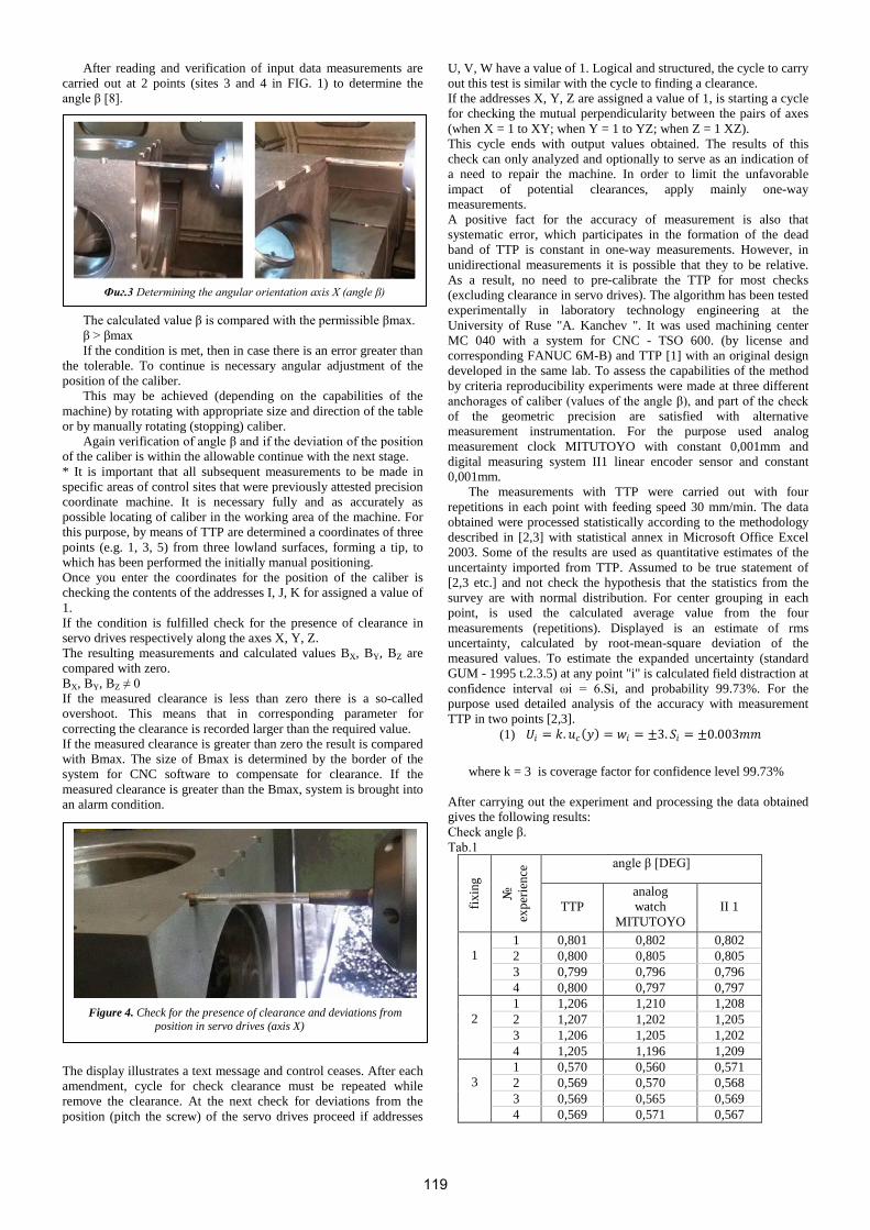
After reading and verification of input data measurements are carried out at 2 points (sites 3 and 4 in FIG. 1) to determine the angle β [8].

The calculated value β is compared with the permissible βmax. β > βmax If the condition is met, then in case there is an error greater than

the tolerable. To continue is necessary angular adjustment of the position of the caliber.

This may be achieved (depending on the capabilities of the machine) by rotating with appropriate size and direction of the table or by manually rotating (stopping) caliber.

Again verification of angle β and if the deviation of the position of the caliber is within the allowable continue with the next stage. * It is important that all subsequent measurements to be made in specific areas of control sites that were previously attested precision coordinate machine. It is necessary fully and as accurately as possible locating of caliber in the working area of the machine. For this purpose, by means of TTP are determined a coordinates of three points (e.g. 1, 3, 5) from three lowland surfaces, forming a tip, to which has been performed the initially manual positioning. Once you enter the coordinates for the position of the caliber is checking the contents of the addresses I, J, K for assigned a value of 1. If the condition is fulfilled check for the presence of clearance in servo drives respectively along the axes X, Y, Z. The resulting measurements and calculated values BX, BY, BZ are compared with zero. BX, BY, BZ ≠ 0 If the measured clearance is less than zero there is a so-called overshoot. This means that in corresponding parameter for correcting the clearance is recorded larger than the required value. If the measured clearance is greater than zero the result is compared with Bmax. The size of Bmax is determined by the border of the system for CNC software to compensate for clearance. If the measured clearance is greater than the Bmax, system is brought into an alarm condition.

The display illustrates a text message and control ceases. After each amendment, cycle for check clearance must be repeated while remove the clearance. At the next check for deviations from the position (pitch the screw) of the servo drives proceed if addresses

U, V, W have a value of 1. Logical and structured, the cycle to carry out this test is similar with the cycle to finding a clearance. If the addresses X, Y, Z are assigned a value of 1, is starting a cycle for checking the mutual perpendicularity between the pairs of axes (when X = 1 to XY; when Y = 1 to YZ; when Z = 1 XZ). This cycle ends with output values obtained. The results of this check can only analyzed and optionally to serve as an indication of a need to repair the machine. In order to limit the unfavorable impact of potential clearances, apply mainly one-way measurements. A positive fact for the accuracy of measurement is also that systematic error, which participates in the formation of the dead band of TTP is constant in one-way measurements. However, in unidirectional measurements it is possible that they to be relative. As a result, no need to pre-calibrate the TTP for most checks (excluding clearance in servo drives). The algorithm has been tested experimentally in laboratory technology engineering at the University of Ruse "A. Kanchev ". It was used machining center MC 040 with a system for CNC - TSO 600. (by license and corresponding FANUC 6M-B) and TTP [1] with an original design developed in the same lab. To assess the capabilities of the method by criteria reproducibility experiments were made at three different anchorages of caliber (values of the angle β), and part of the check of the geometric precision are satisfied with alternative measurement instrumentation. For the purpose used analog measurement clock MITUTOYO with constant 0,001mm and digital measuring system II1 linear encoder sensor and constant 0,001mm.

The measurements with TTP were carried out with four repetitions in each point with feeding speed 30 mm/min. The data obtained were processed statistically according to the methodology described in [2,3] with statistical annex in Microsoft Office Excel 2003. Some of the results are used as quantitative estimates of the uncertainty imported from TTP. Assumed to be true statement of [2,3 etc.] and not check the hypothesis that the statistics from the survey are with normal distribution. For center grouping in each point, is used the calculated average value from the four measurements (repetitions). Displayed is an estimate of rms uncertainty, calculated by root-mean-square deviation of the measured values. To estimate the expanded uncertainty (standard GUM - 1995 t.2.3.5) at any point "i" is calculated field distraction at confidence interval ωi = 6.Si, and probability 99.73%. For the purpose used detailed analysis of the accuracy with measurement TTP in two points [2,3].

(1) 𝑈𝑈𝑖𝑖 = 𝑘𝑘.𝑢𝑢𝑐𝑐(𝑦𝑦) = 𝑤𝑤𝑖𝑖 = ±3. 𝑆𝑆𝑖𝑖 = ±0.003𝑚𝑚𝑚𝑚

where k = 3 is coverage factor for confidence level 99.73%

After carrying out the experiment and processing the data obtained gives the following results: Check angle β. Тab.1

fixin

g

№

expe

rienc

e angle β [DEG]

TTP

analog watch

MITUTOYO

II 1

1

1 0,801 0,802 0,802 2 0,800 0,805 0,805 3 0,799 0,796 0,796 4 0,800 0,797 0,797

2

1 1,206 1,210 1,208 2 1,207 1,202 1,205 3 1,206 1,205 1,202 4 1,205 1,196 1,209

3

1 0,570 0,560 0,571 2 0,569 0,570 0,568 3 0,569 0,565 0,569 4 0,569 0,571 0,567

Фиг.3 Determining the angular orientation axis X (angle β)

Figure 4. Check for the presence of clearance and deviations from

position in servo drives (axis X)

119

Received experimental data is examined to detect big errors. Used is a variation of a criterion Dickson. It is convenient and

powerful enough for this purpose. (2) 𝐾𝐾𝐾𝐾 = (𝑌𝑌𝑛𝑛 − 𝑌𝑌𝑛𝑛−1)(𝑌𝑌𝑛𝑛 − 𝑌𝑌1) < 𝑍𝑍𝑞𝑞 ,

where KD is estimated coefficient at criterion of Dickson; Y1, .... , Yn-1, Yn - variation order data; Yn - inspected member of the variation order; Zq - critical value of criteria according to the respective number

of items in the order (in this case 4). KD=0.5<Zq=0.76

To confirm the first result (second examination) is used and the criterion of Romanovsky, which is convenient for data of up to 20 items:

(3) 𝐾𝐾𝐾𝐾 = �𝑌𝑌�−𝑌𝑌𝑖𝑖𝑆𝑆� = 𝛽𝛽 ≤ 𝛽𝛽𝛼𝛼 ,𝑛𝑛 ,

where KR = β calculated coefficient based on the criterion of Romanowski;

Y -Estimated average value (calculated average of the variation order);

Yi - Checked value; S - estimate standard deviation; βα,n - Critical value. The result: KR=1.25 < βα,n = 1.72 And with both criteria was found that among the checked values

of the selected variational lines are not available, which should be excluded as big errors. Therefore it must be assumed that this also applies to all other lines of experiments having less estimate standard deviation.

Experimental verification is made and for any deviation from perpendicularity of the axis Y toward X axis (angle α1) on the same machine.

Calculations used the average that is obtained from 4 repetitions of measurements at each control point.

In calculating the deviation is used dependence [8]: 𝛼𝛼1 = 𝛽𝛽1 + 𝛾𝛾1 ± 𝛿𝛿1, β1 is the angular deviation in the location of the caliber (in this

case β1 = 0) γ1 is measured deviation from perpendicularity of the control

surfaces (sites 2 and 4) of caliber in its appraisal. (In this case γ1 = 0,127⁰) δ1 = 0,135⁰) is obtained by TTP control. Therefore, in this case: α1 = 0,008⁰ The result can be used by the user to assess the geometric

accuracy of the machine on this indicator. Data can be use in some decisions, representing the development proposed by [2,3,5,6,7].

3. Conclusion Based on the results obtained can be formulated as follows: - The experimental survey confirmed the ability of the

developed theoretical model to control of deviations in the geometrical precision of OC;

- The developed algorithm and control programs provide necessary detail and flexibility of controls for user;

- The implementation of control through this approach provides sufficient accuracy of measurement and is easy to apply in terms of small businesses.

4.Literatura [1] Dimitrov, D. 3D touch probe. International Conference

AMTECH-07, Gabrovo, 2007, p.223-226 [2] Karachorova V. Dimitrov D. Opportunities for automatic

self-test of machining centers. SC RU and SU - 2011, Ruse Volume 5, Series 2, Mechanics and engineering technology,, Ruse, 2011, p. 78 ÷ 82

[3] Karachorova V. Research accuracy in coordinate measurements of machining centers SC RU and US - 2012, Ruse, mechanics and engineering technologies, Rousse, 2012, RU "Angel Kanchev" Rousse, 2012, p.99-103

[4] Nenov D D. Dimitrov, V. Karachorova. Working caliber to verify the geometric precision machining centers. Conference - RU & US'13 in Bulgaria, mechanics and engineering technologies RU "Angel Kanchev", 2013, Rousse, 2013, p.48-51

[5] Hadjiiski P. W. Kaldashev O. Karakostopulo, Measurement errors by identifying and compensating them with postprocessor at four and five axis processing magazine. Mechanical Engineering and Machine, 2013, tom19, str.23-27, ISSN1312-8612

[6] Dimitrov, D., Karachorova, V., Szecsi, T., System for Controlling the Accuracy and Reliability of Machining Operations on Machining Centres.// Procedia Engineering, 2013, No 63, p. 108-114, ISSN 18777058

[7] Georgiev V, I. Chetrokov, S. Lilov, S.Salapateva. Information technologies and control of technological processes, Journal of the Technical University at Plovdiv "Fundamental Sciences and Applications" Vol.13 (6) 2006 Anniversary Scientific Conference ' 2006, p.111-118.

[8] Dimitrov D, V. Karachorova, G. Nenov Mathematical model for determining of the non perpendicularity of linear axes of machining center using a prismatic caliber, SCIENTIFIC PROCEEDINGS of the scientific technical union of mechanical engenering, 2016, number 23/209, p. 78-81, ISSN 1310-3946.

120

RESEARCH THE ACCURACY OF THE GROUP APPROACH FOR RAPID DETERMINATION COST OF THE MACHINING PRODUCT

ИЗСЛЕДВАНЕ ТОЧНОСТТА НА ГРУПОВ ПОДХОД ЗА ЕКСПРЕСНО ОПРЕДЕЛЯНЕ НА СЕБЕСТОЙНОСТТА НА МАШИНОСТРОИТЕЛНО ИЗДЕЛИЕ

Assist. Dimitrov D. PhD.1, M.Sc. Malchev N.2, M.Sc. Karachorova V.1

Faculty of Mechanical and Manufacturing Engineering – University of Ruse “Angel Kanchev”, the Republic Bulgaria 1

SPARKY GROUP - Ruse Company, Inc., the Republic Bulgaria 2

ddimitrov@uni-ruse.com

Abstract:In the publication are presented studies to determine the accuracy of the group approach in calculating the cost of technological engineering products. For this purpose, the cost price of a specific item is calculated by applying the developed approach and the group is compared with the actual cost. The results obtained show that the use of group approach enables a comparatively fast and sufficiently precise calculation of the technological cost of machine products.

Keywords MECHANICAL ENGINEERING, TECHNOLOGY COST, OFFER

1. Introduction

There are different methods to calculate project cost of the technology of machine products. Each of them has advantages and disadvantages. With approximate methods the results are obtained quickly, but the accuracy is low. The detailed methods can achieve high accuracy, but their productivity is low. Both indicators are highly dependent on subjective factors. At the same time in the development of offer is very important to achieve a high accuracy in calculations in the shortest possible time. It turns out that for some types of production may be appropriate application of the so-called. group approach. The essence of this approach is discussed in [2,4]. Through this publication, the results were obtained in the experimental verification and testing system for calculating cost accounting.[1,3,4]

2. Exhibition System cost accounting The system was developed in accordance with the

characteristics of products, production program, organization of production and technological equipment of the company SPARKY AD - Ruse.

To implement the approach was made following: 1. Classification and grouping of products. 2. Selection of real or elaboration of imaginary (virtual)

complex article for each group. 3. Develop a group process for complex product. 4. Calculation of the technological cost of the complex product. 5. Automated calculate the cost of a particular product using a

model. 6. Comparing the results with cost obtained by individually

detailed non-automated calculation. In carrying out the various stages used software utility. For

“Disassembly "(fragmentation) of any representative of its component parts used graphics software for 3D modeling SolidWorks. Automated calculations at this stage is perfectly suited WordExel. For testing of the system used several products from the production company. By systematization, classification and grouping elementary details, surfaces and processes, the products are distributed and grouped into groups with conditional designations A, B, C, etc. Individual parts belonging to one group are denoted by two letters (the first name of the group, while the second is symbol P for part) and a number representing the serial number of the product. For example for group A the parts are indications AP1, AP2, AI3, etc. Similarly parts of group B are BP1,

BP2, BP3, etc. In calculating cost CC are reported only the cost of electricity and labor. Labour costs include wage costs and depreciation of used machines. The calculation is performed by three representatives of the company. They are conventionally indicated with X, Y and Z and are not randomly selected.

In case X is the leader of the technology department. He has many years of production experience and good knowledge of design and technological features of each of the selected products.

The employee Y is a technologist in the technology department. He has worked three years in office and partially known structural and technological features of some of the selected products.

The employee Z has experience about 1 year. Due to the minimum practical experience he can rely principally on its theoretical training in education.

The experiment was made in the following sequence. Initially, each officer calculated CC cost of products using the

system. The next stage is the cost CM be calculated as approved and

known to all methods. To assess the effectiveness of the system used two indicators: Accuracy - The results of both calculations were compared by

calculating the relative error. For the "real" accepted value obtained by the traditional method of leader X.

Productivity - For each estimated cost is recorded time T (working hours) that has been spent on the activity by the employee using the system Tc and using traditional methods Tm. It estimates the absolute and relative difference in productivity.

The values obtained are presented in Table 1. In completing the table used computational respective

dependencies. To calculate the relative error for each employee:

𝐾𝐾𝐶𝐶(x, y, z) =|𝐶𝐶𝐶𝐶(𝑥𝑥,𝑦𝑦, 𝑧𝑧) − 𝐶𝐶𝑀𝑀|

𝐶𝐶𝑀𝑀(𝑥𝑥)

The absolute difference between spending time using classical

methods (TM) and system (Tc) of each employee (X, Y, Z) is calculated with the relationship:

∆Т(𝑥𝑥,𝑦𝑦, 𝑧𝑧) = |𝑇𝑇𝑀𝑀(𝑥𝑥 ,𝑦𝑦 ,𝑧𝑧) − 𝑇𝑇𝐶𝐶(𝑥𝑥 ,𝑦𝑦 ,𝑧𝑧)|

Climate productivity at relatively comparing the times of each

employee in both methods is obtained dependence:

Кт, 𝑖𝑖 =Км, 𝑖𝑖Кс, 𝑖𝑖

121

Depending “i” is X, Y or Z.

3.Conclusion Analysis of the table gives rise to the following conclusions:

1. The relative error for leader X is dashing R = 0.094. 2. The maximum relative error in the operation of X is below 10% and occurs only in one case. 3. The maximum error for the entire experiment in the work of Z. It was obtained once and is under 16%. 4. The total expenditure of time (all parts) for leader X using system is 4.25 hours, and without system is 56 hours. Therefore, consumption of time is reduced an average of 12.5 times. 5. The total expenditure of time (all parts) for employee Y at using the system is 32.5 hours, but without system is 161.5 hours. Therefore, the cost of time is reduced by an average of 4.1 times.

4.Literatura [1] Dimitrov D, etc. Malchev. Unification of processes in wide range of production of large thin-walled parts. Q: SC Ruse University and the Union of Scientists in Bulgaria - Rousse branch 2015, Rousse, 2015, p. 179-183 [2] Zamfirov I., D. Dimitrov, St. Koleva. Group and Standard Process - textbook, Rousse, 2013, Publishing Center of the University of Ruse, p. 132, ISBN 978-954-712-580-3 [3] Malchev N. Exploring the possibilities of developing a quick offer in wide range of production. Q: Nauchna conference Ruse University and the Union of Scientists in Bulgaria - Rousse branch 2015, Rousse, 2015, p. 175-178 [4] D. Dimitrov, N. Malchev. Group approach for express offer the determination of cost price of mechanical engineering product in small scientific proceedings, SCIENTIFIC PROCEEDINGS of the scientific technical union of mechanical engenering, 2016, number 23/209, p. 75-77, ISSN 1310-3946.

Tabl.1

АP1 АP2 АP3 АP4 АP5 АP6 АP7

Сс, [lv.]

X 359,69 450,66 582,15 596,38 672,11 796,27 571,97

Y 368,75 462,32 595,26 618,13 661,78 786,28 575,44

Z 379,2 498,18 638,75 537,26 601,23 847,43 605,12 См, [lv.] X 327,66 455,29 579,67 606,32 646,74 785,34 553,48

Кс

X 0,098 0,010 0,004 0,016 0,039 0,014 0,033

Y 0,125 0,015 0,027 0,019 0,023 0,001 0,040

Z 0,157 0,094 0,102 0,114 0,070 0,079 0,093

Тс, [h]

X 0,75 0,75 0,50 0,50 0,50 0,75 0,50

Y 5,50 5,50 5,00 4,50 4,50 4,00 3,50

Z 9,50 8,50 8,00 7,00 7,50 7,50 6,50

Тм, [h]

X 9,50 8,00 7,00 7,50 7,50 8,50 8,00

Y 22,50 24,00 24,50 20,50 22,50 26,50 21,00

Z 37,50 38,00 35,00 31,00 30,00 36,00 29,00

ΔТ, [h]

X 15,75 17,25 17,50 15,50 17,00 18,25 16,00

Y 17,00 18,50 19,50 16,00 18,00 22,50 17,50

Z 28,00 29,50 27,00 24,00 22,50 28,50 22,50

Кт

X 11,7 9,7 13 14 14 10,3 15

Y 3,1 3,4 3,9 3,6 4,0 5,6 5,0

Z 2,9 3,5 3,4 3,4 3,0 3,8 3,5

122

SELECTING THE OPTIMUM VARIANT OF THE SHEAR DRAWING PROCESS FOR LOW-CARBON STEEL

ВЫБОР ОПТИМАЛЬНОГО ВАРИАНТА ПРОЦЕССА ВОЛОЧЕНИЯ СО СДВИГОМ

НИЗКОУГЛЕРОДИСТОЙ СТАЛИ

Prof., D. Sc. Tontchev N.1, Lead. Res., Dr. Semenov V.I.2,3, Jun. Res. Raab A.G.2, Assoc. Prof. Kamburov V.4

1«Todor Kableshtov» Higher School of Transport, Sofia, Bulgaria

2Ufa State Aviation Technical University, Ufa, Russia 3Institute of Oil and Gas Technologies and Novel Materials, Ufa, Russia

4 Technical University of Sofia, Bulgaria

Abstract. With the help of computer simulation in the DEFORM-3D software, there was performed a virtual full factorial experiment of the process of shear drawing. In the course of the experiment, the effect of independent parameters (drawing speed, die rotation rate, die angle and friction factor) on the strain intensity was evaluated. As a result of the experiment, a regression equation was derived and the most significant individual factors and their combinations, influencing the response parameters, were determined. Also, comparative results were presented for the processes of regular drawing and shear drawing. It was demonstrated that the process of shear drawing has a higher efficiency from the point of view of strain intensity. KEY WORDS. SIMULATION, SHEAR DRAWING, VIRTUAL FULL FACTORIAL EXPERIMENT, PLANNING MATRIX, STRAIN INTENSITY.

1. Introduction At present, there is interest in studies in the area of

enhancement of metals' strength due to structure refinement down to the submicrocrystalline (SMC) size through severe plastic deformation (SPD) processing [1]. Among the SPD techniques are equal-channel angular pressing (ECAP) [2, 3] and its advanced variation – ECAP-Conform [4], which was designed for the fabrication of long-length billets with a bulk SMC structure and enables creating prerequisites for the practical implementation of SPD processing.

The technical process based on structure refinement through SPD processing and implemented with the use of an ECAP-Conform facility is an efficient method to increase the strength of metals and alloys. However, it has several drawbacks:

1) muti-cycle processing is required to produce high levels of accumulated strain in the processed material;

2) long-length rods with a square section are produced; 3) additional post-deformation treatment, e.g. drawing, is

required to produce rods with a round section. To eliminate the above-mentioned drawbacks, the method of

shear drawing was proposed. Deformation accompanied by a change in the mechanical properties of a metal is effected due to drawing and rotation of an eccentric drawing die, which provides additional shear deformation [5].

It is difficult to describe the behavior and prediction of the process of shear drawing due to the lack of sufficient full-scale experiments, since work at a physical experiment is rather time-consuming and costly in terms of capital investments.

In research and practical activity, a prominent place is held by numerical methods for the study of complex processes, inculding simulation with the use of cutting-edge software products. The efficiency of the use of simulation methods and solution of engineering tasks grows substantially, if at the stage preceding the design of actual technological processes, conditions are created for the evaluation of the most important parameters.

Application of mathematical methods is one of the most rational approaches to the solution of tasks related to the efficiency of evaluation of non-conventional metal forming processes. In this connection, it is reasonable to perform numerical simulation with the use of planning of a virtual full-factorial experiment (FFE) [6].

The advantage of a FFE is the ability to describe a process with full observation of the physical experiment's alogorythm, taking into account the set assumptions. FFE is the most easily implementable method among the numerous methods of physical experiment. The aim of applying FFE is to produce a linear

mathematical model of a process, which will help to define further strategy in performing a real experiment.

Thus, the aim of simulation is to perform a virtual process of shear drawing with the use of FFE, and to reveal the most efficient conditions for producing long-length SMC semi-products.

2. Experimental procedure In order to obtain the fullest information about the studied

dependencies, the authors used FFE when performing the simulation. Experiment planning is a procedure of selecting the number and conditions of tests that are necessary and sufficient for producing the mathematical model of a process [7]. Here, it is important to consider the following: tendency for the minimization of the number of tests; simultaneous variation of all variables defining the process; selection of a clear strategy that enables making grounded decisions after each series of experiments. Prior to planning a full-scale experiment, it is necessary to collect additional information about the studied object, using the skills and knowledge obtained earlier in previous investigations or described in literature [8].

The experiment planning was performed for the method of processing of long-length rods with a round section from low-carbon steel. The facility for shear drawing consists of two eccentric drawing dies, one of which rotates [5]. Its schematic illustration is presented in fig.1.

Fig. 1. Drawing dies for shear drawing.

The object of study is low-carbon steel with a carbon content

of 0.1 %. The rheological properties of the steel were entered when developing the numerical model [9].

123

To perform the numercial simulation, the standard application software package (ASP) DEFORM-3D was used.

With a view to perform modeling and factorial experiment in the DEFORM-3D ASP, three-dimensional models of dies with different angles of the working part were designed in advance in the KOMPAS-3D software.

Accepted assumptions 1) The billet material in the initial state is isotropic and

has no initial stresses and strain; 2) The temperature of the deformation environment is

accepted as 20ºС; 3) The tool is absolutely rigid, and the tool's geometry is taken

into account automatically; 4) The initial billet's material is accepted as ductile; 5) For the simulation, 100 steps are selected, taking into account

the full passage of a billet in the dies and the generation of a stable result; 6) The billet is divided into 43553 trapezoidal elements.

At the stage of the simulation task preparation, the most significant factors influencing strain intensity in the process of shear drawing at room temperature are the die angle, the drawing speed, the rate of the die's rotation around its axis and the tribological parameters of the billet's contact with the tool. In this connection, it was decided to perform a virtual FFE using a two-level model with four unknown variable factors with subsequent formalization of the obtained results in the form of regression equation and optimization of the selected factors.

Thus, as independent variables in the process of shear drawing, characterizing the execution of the process and its efficiency, from the point of view of strain intensity we selected the wire drawing speed V (Х1), the die rotation rate ω (Х2), the die angle α (Х3) and the friction factor fтр. (Х4). The parameter of response (or dependent variable) determined the material's strain intensity (Y).

The factors were varied at two levels. The variation intervals of variable factors and their values in full scale are presented in table 1.

Table 1 . Levels of factors

Factors X1 (V, m/min.) X2 (ω, min-1) X3 (α, grad.) X4 (fтр.) Basic level (Xi) 20 350 15 0.50 Variation interval (∆Xi) 10 50 5 0.25 Upper level (xi = 1) 30 600 20 1 Lower level (xi = – 1) 10 100 10 0

The number of tests N was determined from the number of

factors k in accordance with the expression:

1622 4 === kN (1) It is necessary to determine such values of V, ω, α, fтр.,

under which the strain intensity ε in the range of 1 to 3 (1 ≤ ε ≤ 3) will be provided.

3. Experiment results and discussion

The mathematical model after running tests of full factorial

experiment has the following form:

y=b0+b1x1+b2x2+…+b12x1x2+b13x1x3+…+b123x1x2x3+b124x1x2x4+ …+b1234x1x2x3x4, (2)

where bi is regression coefficients. To calculate the coefficients of this model, we constructed

an expanding matrix of planning and test results (table 2).

Table 2 . Expanded matrix of the plan 24 and test results

Test No. х0 х1 х2 х3 х4 х1х2 х1х3 х1х4 х2х3 х2х4 х3х4 х1х2х3 х1х2х4 х1х3х4 х2х3х4 х1х2х3х4 у

1 + + + + + + + + + + + + + + + + 0.30 2 + - + + + - - - + + + - - - + - 0.70 3 + + - + + - + + - - + - - + - - 0.90 4 + - - + + + - - - - + + + - - + 0.50 5 + + + - + + - + - + - - + - - - 0.50 6 + - + - + - + - - + - + - + - + 0.90 7 + + - - + - - + + - - + - - + + 0.60 8 + - - - + + + - + - - - + + + - 0.70 9 + + + + - + + - + - - + - - - - 0.40

10 + - + + - - - + + - - - + + - + 1.50 11 + + - + - - + - - + - - + - + + 1.10 12 + - - + - + - + - + - + - + + - 1.20 13 + + + - - + - - - - + - - + + + 0.70 14 + - + - - - + + - - + + + - + - 0.90 15 + + - - - - - - + + + + + + - - 1.30 16 + - - - - + + + + + + - - - - + 1.00

The regression coefficients were calculated according to

the formula:

N

yxN

ii∑== 1i

ib , (3)

where i = 0, 1, 2, …, 16.

From the calculations, the following general form of the

linear regression equation was obtained:

y=0.825X0+0.0125X1+0.2X2–0.1125X3–0.075X4–0.1625X1X2–0.05X1X3+0.175X1X4– 0.0125X2X3+0.05X2X4–0.0375X3X4+0.05X1X2X3– 0.0875X1X2X4 +0.0X1X3X4+ 0.0625X2X3X4+0.0X1X2X3X4 (4)

124

As a result of implementation of the two-level four-factor model of FFE and identification of the statistical significance of each of the 16 coefficients [10], regression equation (4) assumed the following form:

y=0.825X0+0.2X2–0.1125X3–0.075X4+0.1025X1X2+0.175X1X4–0.0875X1X2X4+ 0.0625X2X3X4 (5)

Here, the hypothesis of the adequacy of mathematical

model (5) in terms of the F-test [6] at a 5% significance level is not discarded.

It can be seen from equation (5) that the strain value is most significantly influenced by the die rotation angle, the die angle and the friction factor, as well as the combined interaction of the drawing speed and the die rotation rate; drawing speed and friction factor; drawing speed, die rotation rate and friction factor; die rotation rate, die angle and friction factor. A combined interaction of the rest of the factors has an insignificant influence on the strain intensity value. It is established that strain intensity increases with increasing die rotation rate and decreasing die angle and friction factor. Also, the response parameter grows as the drawing speed and the die rotation rate are simultaneously increased. A combined increase in the drawing speed and friction factor has a more significant effect on strain intensity. What can be predicted to a lesser degree is the effect on strain intensity of simultaneously three independent variables from the variables considered in this setting: the drawing speed, the die rotation rate and the friction factor, as well as the die rotation rate, the die angle and the friction factor. Also, their cumulative effect is multidirectional. Therefore, complex interactions should be analyzed separately and and in connection with the specific operation conditions of the multi-component system.

It can be seen from equation (5) that the drawing speed on its own has a small effect on strain intensity, but in combination with the die rotation rate, the die angle and the contact conditions in the plastic tribocoupling it can efficiently increase strain intensity.

Thus, it follows that the maximum strain intensity value can be attained under the optimum combination of the drawing rate with other independent parameters considered in this study.

For a more illustrative analysis of the obtained mathematical model, a diagram was built showing the effect of different factors on strain intensity (fig. 2).

It is visible from fig. 2 that the increase in strain intensity grows with increasing die rotation rate. The combination of

deformation speed with the die rotation rate has a substantial effect on the response parameter.

Fig. 2. Effect of significant factors and their interactions:

for the negative values – the response parameter grows as a factor decreases; for the positive values – the response

parameter grows as a factor increases From this it follows that the efficiency of the shear drawing

process depends on the synchronization of these two parameters which need to be considered in combination when designing the technnological process. It can also be seen from fig. 2 that the die angle and the friction factor, as individual parameters, are supposed to decrease for the strain intensity to increase. At the same time, from the analysis of pair and triple interaction effects (Х1Х4, Х1Х2Х4, Х2Х3Х4) it can be seen that the friction factor and the die angle, in combination with the drawing speed and the die rotation rate, have a significant and ambiguous effect on strain intensity, which should also be taken into account when designing the technological process of shear drawing.

Of practical interest is the solution of the optimization task for determining the actual values of independent parameters considered within the virtual experiment of numerical simulation, ensuring the maximum value of strain intensity in the process of shear drawing. This task was solved using the metod of «the steepest ascent» [6].

The steps in the variation of factors were calculated in full scale. With this aim, at first the products of the coefficients and the corresponding variation intervals of these factors were determined, i. e. bi∆Xi, then steps were assigned proportionately to these products. The realization sequence of the steepest ascent stages is shown in table 3.

Table 3 Steepest ascent

Factors Х1 (drawing

speed, m/min)

X2 (die rotation rate,

min-1) X3 (die angle,

deg.) X4 (friction

factor) y (strain intensity)

bi bi∆Xi Step Step after rounding

0.0125 5* 10 10

0.20 10.00

20 50

- 0.1125 - 0.5625 - 1.125 - 2.0

- 0.075 - 0.019 - 0.038 - 0.05

Basic level (Xi) 20 350 15 0.50 Thought test Implemented test Thought test

15 15 15

100 150 200

20 18 16

0.45 0.40 0.35

0.90

Thought test Implemented test Thought test

15 15 15

250 300 350

14 12 10

0.30 0.25 0.20

0.70

Thought test Implemented test Thought test

15 15 15

400 300 500

20 18 16

0.15 0.10 0.12

1.20 1.60

Thought test Implemented test Thought test

15 15 15

550 600 600

14 12 10

0.15 0.10 005

0.70

125

* the value of bi∆Xi for Х1 (drawing speed) is set a priori due to the need to synchronize this factor with the other significant independent parameters admitted to consideration. Here, the step is selected randomly for technological reasons

Some of the thought tests were implemented within the computer model (table 4). The experiment planning using the steepest ascent method demonstrated that in the considered conditions the strain intensity will be the largest under a high die rotation rate (ω ≈ 500 min-1), a small die angle (α ≈ 16o) and a decreasing friction factor (fтр. → min). Here, the axial drawing rate (V), due to its small effect on strain intensity as an individual parameter, was accepted as constant and equal to 15 m/min.

In the framework of the task set for the study, we obtained optimized numerical values of the variable parameters, corresponding to the required value of strain intensity (ε ≥ 1.155).

Simulation of the shear drawing process in the DEFORM-3D environment was performed with the following parameters:

Table 4. The source of data for computer models

Friction factor (according to Siebel) 0.12

Die angle, deg. 16 Drawing speed, m/min 15 Die rotation rate, min-1 500

Given below are the results of numerical simulation

according to the optimized values obtained in the process of the virtual FFE.

Analysis of the billet's strained stated after shear drawing shows that the largest value of ε is attained on the billet's surface (fig. 3b), since this is where the greatest metal deformation takes place, associated with the geometry of the dies and the rotation of one of the dies.

Fig. 3 Pattern of strain intensity distribution in the process of shear drawing: а – in the longitudinal section on the axis; b – in the

longitudinal section on the surface. To estimate the values of strain intensity per one

processing cycle, analysis of the processes of shear drawing and regular drawing was performed.

From the distribution of strain intensities (fig. 4) it can be

seen that per one cycle of shear drawing larger values are obtained than per one cycle of regular drawing.

Fig. 4 Pattern of strain intensity distribution in the transverse section: а – shear drawing; b – regular drawing.

Fig. 5 Distribution of normal forces on the deforming tool. а – shear drawing; b – regular drawing.

Study of the normal forces on the tool demonstrates that as

the die rotates, the forces acting on the tool decrease almost by 2 times, which expands the nomenclature of steels for the

production of the tool and thus may facilitate cheapening of the process (fig. 5).

126

4. Conclusions 1. The virtual FFE using the steepest ascent method in

the process of numerical simulation has enabled identifying the optimum numerical values of independent parameters which ensure the maximum strain intensity value at room temperature. To obtain ε ≈ 1.6, it is necessary to provide a die rotation rate of ω ≈ 500 min-1, a die angle of α ≈ 16 о and a friction factor of fтр. ≈ 0.12 under a rotation speed of V = 15 m/min.

2. Comparative analysis of the processes of shear drawing and regular drawing for steel 10 at room temperature enables reducing the drawing forces almost by 2 times, increasing the maximum values of accumulated strain intensity from 0.5 to 1.6 and, in addition, reducing normal forces on the tool by 1.8 times.

References

[1] R.Z. Valiev, I.V. Alexandrov. Bulk Nanostructured Metallic Materials: Processing, Structure and Properties.– Мoscow: Akademkniga, 2007. – 398 p. (in Russian).

[2] V.M. Segal, V.I. Reznikov, V.I. Kopylov, et al. Processes of Plastic Structure Formation. Minsk: Nauka i Tekhnika, 1994. 232 p. (in Russian).

[3] Segal V.M. Engineering and commercialization of equal channel angular extrusion // Mater. Sci. Eng. A. – 2004; V. 386. P. 269 – 276.

[4] G.I. Raab, R.Z. Valiev, Equal-channel angular pressing of long-length billets. Tsvetnaya Metallurgiya-2000 –No. 5, p.50-53 (in Russian).

[5] Invention patent of the Russian Federation No. 2347633 Method for production of ultrafine-grained semi-finished products by drawing with shear. Publication date 27.02.2009 Authors: G.I. Raab, A.G. Raab. Patent owner: Ufa State Aviation Technical University, patent in force.

[6] F.S. Novik, Ya.B. Arsov: Optimization of Metal Technology Processes by Methods of Experiment Planning, Mashinostroenie, Sofia: Tekhnika, 1980, 304 p. (in Russian).

[7]7Yu.P. Adler, Experiment Preplanning. Мoscow: Znanie. 1978. 72 p. (in Russian).

[8] Yu.P. Adler, Introduction to Experiment Planning. Мoscow: Metallurgiya. 1969. 158 p. (in Russian).

[9] V.G. Sorokin, A.V. Volosnikova, S.A. Vyatkin, et al., Guide to Steels and Alloys. Мoscow: Mashinostroenie. 1989. 640 p. (in Russian).

[10] L.A. Slavutskiy, Fundamentals of Data Registration and Experiment Planning: study guide. Cheboksary: Chuvash State University, 2006. 200 p. (in Russian).

127

VARIOUS WAYS FOR CONTROLLING DIFFERENT TYPES OF DEVICES USING EMG SIGNALS

M.Sc. Eng. Rõbak D.1, Ass. Prof. Penkov I., Ph.D2.

Department of Electrical Power Engineering and Mechatronics – Tallinn University of Technology, Estonia1 Department of Mechanical and Industrial Engineering – Tallinn University of Technology, Estonia2

dmitrirybak@gmail.com, igor.penkov@ttu.ee

Abstract: This study opens up new opportunities for developers and end users to realize an excellent facility of electromyography technology interfacing with different mechatronic devices. The article provides a brief review of the various ways for controlling different types of devices by using human-machine interface with help of electromyography (EMG) technology. How to register EMG signals from human muscular activity and evaluate the electrical potentials with the help of hardware and control the artificial limbs.

Keywords: EMG SIGNALS, ARTIFICIAL LIMBS, MOTION, ENERGY SAVING

1. Introduction The advent of the new technology has opened opportunities to

the computer user interfaces to consider alternative ways to communicate with machines and computer devices and allow users to create an immersive experience in environment virtual reality. This study provides a brief review of the various ways for controlling different types of devices by using human-machine interface with help of electromyography technology.

All the developed devices can be divided into two categories: medical or industrial. The purpose of this research is to find and develop a conceptual solution and combine it in one device. Many people are physically disabled by losing a leg or an arm as a result of an accident or injury. To solve this problem and improve the quality of life of disabled people, optimal ergonomic artificial limbs are being invented. Also, this technology can be used for other purposes, such as for creating different types of controlled equipment and intelligent systems. The user interface for these devices is as a rule derived from graphical interfaces for computers using reduced versions of the hardware devices. At the same time it can be used for controlling teleported machinery in hazardous or extreme conditions that humans must avoid. Over the last years, a number of innovation and development in the field of human computer interfaces have been developed such as the light pens, the drawing tablets, different types of smart phones. All of these devices and interfaces require human assistance in hardware device that translates human movement to a binary numbers that the electronic computer can analyze and process using the software algorithms [22].

This study opens up new opportunities for developers and end users to realize an excellent facility of electromyography technology interfacing with different mechatronic devices. With the help of the EMG technology we can register and evaluate the electrical potentials produced by skeletal muscle cells when these cells electrically or neurologically activated. The EMG signals received are produced by skeletal muscles and can be processed depending on their potential. Since the received impulses have different amplitudes, it is possible to register detailed necessary impulses and evaluate them with a controller, which controls the servomotors [23]. Though electromyography has been used for a long time for commercial prosthetic hands, all of the solutions have limited capabilities. EMG signals recorded from the muscles of the limb were used for extracting kinematic variables (i.e., joint angles) in order to control an anthropomorphic robot in real time. The novelty of the method proposed here can be centered around two main issues that are discussed in [8, 10, 12, 13, 18]. First, the dimensionality reduction is quite significant, since it does not only reveal some interesting aspects regarding the 3-D movements studied, but it also aided the matching between the EMG signals and motion since signal correlations were extracted, and the number of variables was drastically reduced. The latter led to the fact that a simple linear model with hidden states proved quite successful in

the mapping [4, 8, 15, 17]. Concerning EMG signals to arm motion, the 3-D arm motion is somehow constrained by the use of only two independent variables that describe arm motion does not hinder the applicability of the method [11, 16, 19, 20]. This is based on the suggestion of motor synergies, which allows those decoded to be represented back in the high-dimensional space, where four human joint angles are actuated, concluding to motion of the human arm in the 3-D Cartesian space with limited though workspace. The second important issue presented here is that, to the best of knowledge, this is the first time a continuous profile of the 3-D arm motion is extracted using only EMG signals. Most previous works extract only discrete information about motion, while there are some works that estimate continuous arm motion; however, they are constrained to movements or very smooth motions [2, 5].

2. Existing solutions There are many developers and company's solutions using the

EMG technology to control artificial limbs. With quickly development in the world of computer science and EMG technologies are anticipated to be used and integrated with the intelligent mechatronic and robotic systems. Signal amplification and filtering is the basic in processing and application systems. In nowadays many scientist and researchers searching for better amplification and filtering circuit design that is able to meticulously capture surface EMG signals and for the current applications is still a challenging [22].

In the electromyography technologies the characteristic of the amplifiers and filters determine the quality of EMG signals and plays the significant role. Thalmic Labs company offer new solution, device which can control PC interface using the EMG technology. The solution consist of the high input impedance amplifier connected to electrodes which attached to the human skin, an anti aliasing filter, microcontroller which digitize and process the EMG signals, Bluetooth communication module send the processing results to the other processing unit [23]. This device is attached to the human wrist on the adjustable bracelet, which is able to accommodate to all users and can be hidden under clothes. The surface electrodes are attached on the skin surface to get the electrical potential generated by muscle cells when these cells neurologically activated. Simple controller also can be used within a multimodal interface. When device detected electrical potentials produced by skeletal muscle cells (EMG signals), the controller sends a processing results wirelessly to the processing unit, such as smart phone or PC. In practical applications, EMG signals amplification and filtering plays the significant role, during the process the device have to receive best quality of EMG signals as possible and decrease the noise component from the signal. Applying this device with multimodal interfaces, system can also deliver high- resolution information and display using a GUI and communicate with other devices. This device can be used and

128

integrated with the intelligent mechatronic and robotic systems. A standard machine learning method (namely, a Support Vector Machine) is used to build a point-to-point map between muscle activity and hand position/orientation/grasping force. The map relies on gravity compensation and rather low movement speed, which enforces a many-to-one relationship between the EMG signals and the position. It was noted that the performance of the system is considerably higher when a task-oriented training modality is used. Furthermore, the human-friendly control architecture used in combination with the robot enables the operator to be within the workspace of the robot and interact with it. This feature makes the system suitable for a variety of applications in which physical interaction between humans and robots occurs [1, 23].

Fig. 1. (Top) The demonstration of MYO device

(https://www.thalmic.com/en/myo/) [3].

Fig. 2. The demonstration of OttoBock wrist

(http://www.ottobock.com/) [14].

In our days different types of assistive prostheses and wheelchairs are controlled using EMG technology. Many companies today offer solutions in the field of commercial prosthetic. The most advantageous solution by the Otto Bock company has offered a new prosthetic system that assures fast and secure data transmission, using an intelligent Axon-Bus system. The Axon-Bus itself is a new Otto Bock development in the field of exoprosthetics, derived from safety-related bus systems in the aviation and automobile industries – a true innovation in terms of the process and the results. The research focused on small size artificial limbs and filtering circuit design for processing surface EMG signals from electrical activity produced by skeletal muscles for command and controls the artificial limb movement. The control described has a high level of accuracy, such that a small object can be repeatedly grasped, carried around, and released. Muscle activity is gathered using nine surface electromyography electrodes. No

precise placement of the electrodes is required, and no model of the human arm/hand is employed, making the system essentially subject-independent. EMG signals are weak and with the untended noises, EMG signals have to be gently processed until using for any health care solutions. The advantage is that it constitutes a self-contained data transmission system with perfectly harmonized components. The individual components "communicate" with each other perfectly, eliminating losses in terms of data transmission, speed and functionality [9, 14, 20].

3. Ways for improvement Many companies and researchers are developing practical

applications using muscle activity contraction, especially in field of interfaces for people with limited capabilities. The main challenge for the design researchers and developers of hardware and software controlling using EMG signals are high speed of operation, sufficient gap force, mechanical strength, low power consumption, less weight and good computation of software algorithms capability with compatible to control hardware. As revealed by an overview of other developers and company solutions, using the EMG technology to control artificial limbs for people with probability limitations or disability, focus in my further research will be to find and develop a conceptual solution and combine the categories involved into one device. Derived from the limited capabilities of other developer’s solutions, the subjects for further research are:

• Low capacity batteries • Weight and mobility • Slow motion speed • Possibility of sensation

There is need in advanced algorithms to be developed to attract useful neural information. Problem, which is still largely open using the EMG technology to control artificial limbs and to have an opportunity of sensation. The advent of the new technology area of human machine interface considered as priority well is based on EMG technologies. The aim of the future research work to create an integrated system that can use signals coming from the artificial sensors of the robotic manipulator to the human and stimulate the nervous system, using a hybrid controller. Weight and mobility of low capacity batteries is another subject to further research. One of the innovative aspects is the combined use of electromyography to relay information for controlling artificial limbs and to have an opportunity of sensation. There is a great need in all of these devices and interfaces which can required human assistance in hardware device of a reliable and robust control for the myoelectric hardware so that it can be implemented in real-time. EMG is a relatively new technology there is substantial unused potential and it is very beneficial to study the EMG technology for controlling multi function prostheses.

Conclusions The new EMG technologies will bring a solutions to a medical

problems caused by the existing ergonomically incorrect designed devices. As the world population is growing, prostheses for aging population will become a very important field. Innovation and development in the world of prosthesis is a very wide field where the EMG technology has a significant role.

The purpose of this research is to give an attempt to the motivation of the new researchers to the contribution in the field of EMG technology. Some ways for enhancement of the devices can be energy saving, decreasing of mass and size parameters and improvement of feedback registration.

129

Acknowledgments

This research work has been supported by Estonian Archimedes Foundation (project „Doctoral School of Energy and Geotechnology III“).

References

1. B. Lim, S. Ra, and F. Park, “Movement primitives, principal component analysis, and the efficient generation of natural motions” Proc. IEEE Int. Conf. Robot. Autom. pp. 4630–4635, 2005.

2. P. K. Artemiadis and K. J. Kyriakopoulos, “EMG-Based Control of a Robot Arm Using Low-Dimensional Embeddings.” Robotics, IEEE Transactions on 26.2, pp. 393-398, 2010.

3. https://www.thalmic.com/about/Nov. 2016. 4. P. K. Artemiadis and K. J. Kyriakopoulos. An emg-based

robot control scheme robust to time-varying EMG signal features. IEEE Transactions on Information Technology in Biomedicine, 14(3), pp. 582-588, 2010.

5. Y. Koike and M. Kawato, “Estimation of dynamic joint torques and trajectory formation from surface electromyography signals using a neural network model,” Biol. Cybern., vol. 73, pp. 291–300, 1995.

6. O. Fukuda, T. Tsuji, M. Kaneko, and A. Otsuka, “A human-assisting manipulator teleoperated by EMG signals and arm motions,” IEEE Trans. Robotics and Automation, vol 19, no. 2, pp. 210-222, 2003.

7. C. Castellini and P. van der Smagt. Surface EMG in advanced hand prosthetics. Biological Cybernetics, 100(1), pp. 35-47, 2008.

8. P. K. Artemiadis and K. J. Kyriakopoulos. A switching regime model for the emg-based control of a robot arm. IEEE Transactions on Systems, Man, and Cyberneticspart B: Cybernetics, 41(1), pp. 53-63, 2011.

9. E. Cavallaro, J. Rosen, J. C. Perry, S. Burns, and B. Hannaford, ”Hillbased model as a myoprocessor for a neural controlled powered exoskeleton arm - parameters optimization,” Proceedings of the IEEE International Conference on Robotics and Automation, Barcelona, Spain, April 2005.

10. A. Chatterjee, P. Chaubey, J. Martin, and N. Thakor, "Testing a prosthetic haptic feedback simulator with an interactive force matching task," J Prosthet Orthot, vol. 20, pp. 27-34, 2008.

11. C. Castellini, E. Gruppioni, A. Davalli, and G. Sandini. Fine detection of grasp force and posture by amputees via surface electromyography. Journal of Physiology (Paris), 103(3-5), pp. 255-262, 2009.

12. C. E. Stepp and Y. Matsuoka, "Relative to direct haptic

feedback, remote vibrotactile feedback improves but slows object manipulation," in 32nd Annual International Conference of the IEEE Engineering in Medicine and Biology Society, Buenos Aires, Argentina, pp. 2089 - 92, 2010.

13. R. T. Verrillo, "Vibration Sensation in Humans," Music Perception, vol. 9, pp. 281-302, Spring 1992.

14. http://www.livingwithmichelangelo.com, Nov. 2016. 15. A. V. Hill, “The heat of shortening and the dynamic constants

of muscle,”in Proc. R. Soc. Lond. Biol., pp. 136–195, 1938. 16. E.Cavallaro, J. Rosen, J. C. Perry, S.Burns, and B. Hannaford,

“Hill-based model as a myoprocessor for a neural controlled powered exoskeleton armparameters optimization,” in Proc. IEEE Int. Conf. Robot. Autom., pp. 4514–4519, 2005.

17. F. E. Zajac, “Muscle and tendon: Properties, models, scaling, and application to biomechanics and motor control,” in Proc. Crit. Rev. Biomed. Eng., vol. 17, Boca Raton, FL: CRC, pp. 359–411, 1989.

18. R. J. Triolo and G. D. Moskowitz, “The theoretical development of a multichannel time-series myoprocessor for simultaneous limb function detection and muscle force estimation,” IEEE Trans. Biomed. Eng., vol. 36, pp. 1004–1017, 1989.

19. A. d’Avella, A. Portone, L. Fernandez, and F. Lacquaniti, “Control of fast-reaching movements by muscle synergy combinations,” J. Neurosci., vol. 25, no. 30, pp. 7791–7810, 2006.

20. C. E. Stepp, B. T. Dellon, and Y. Matsuoka, "Contextual effects on robotic experiments of sensory feedback for object manipulation," in 3rd IEEE RAS & EMBS International conference on Biomedical Robotics and Biomechatronics, Tokyo, pp. 58-63, 2010.

21. J. Zhao, Z. Xie, L. Jiang, H. Cai, H. Liu, and G. Hirzinger, ”Levenberg-Marquardt based neural network control for a five-fingered prosthetic hand,” Proceedings of the IEEE International Conference on Robotics and Automation, Barcelona, Spain, 2005.

22. J. Vogel, C. Castellini and P. van der Smagt, “EMG-Based Teleoperation and Manipulation with the DLR LWR-III,” IEEE/RSJ International Conference on Intelligent Robots and Systems, San Francisco, CA, USA, 2011.

23. Jingpeng Wang School of Engineering and Advanced Technology Massey, New Zealand, Liqiong Tang School of Engineering and Advanced, John E Bronlund School of Engineering and Advanced Technology ,“Surface EMG Signal Amplification and Filtering” IEEE/RSJ International Journal of Computer Applications (0975 – 8887).

130

THE CUSTOMS LOGISTICS CONCEPT FOR THE SOUTH CAUCASUS TRANSPORT TECHNOLOGICAL SYSTEMS

КОНЦЕПЦИЯ ТАМОЖЕННОЙ ЛОГИСТИКИ ТРАНСПОРТНО-ТЕХНОЛОГИЧЕСКИХ СИСТЕМ

ЮЖНОГО КАВКАЗА

Prof. Dr. Kochadze T., Dr. Tsetskhladze A., Doctoral candidate Gudadze A. Akaki Tsereteli state University - Kutaisi, Georgia

E-mail: Temko1954@mail.ru , alex.tsts75@gmail.com , predatori.ag@gmail.com Abstract: South Caucasus with its geopolitical position and diversity of natural resources is a unique region in the world. A concrete expression of this fact is the EU's “TRACECA” project, which binds the Central Asia, Caspian and Black Sea basin states to one another. This line the Eurasian freight logistics corridor runs through the South Caucasus, which guarantees the economic growth and stability in countries of the region. Strengthening the transit capacity of the South Caucasus countries and improving overall competitiveness of transport corridor will be contributed by the development and formation of a new concept of a single transport and logistics system - the regional customs logistics.

In order to allow fast, safe and efficient movement of commodity flows through the South Caucasus transport corridor, the regional customs logistics should create a single standard of customs processing of freight. This can be accomplished within the “ASYCUDA World” program by creating the appropriate module. KEY WORDS: GEOPOLITICAL POZITION; EURASIAN TRANSPORT CORIDOR; CUSTOMS LOGISTIC

1. Introduction

Enhancement of global trade and economic relations mostly depends on the development of the new trade routes. In the modern era, special attention is being accorded to the idea of developing transnational trade routes, since quantity of cargo is growing and trade and economic relations are characterized by the enhanced intensity. In these conditions, development and implementation of a

new silk road project became more relevant, a special portion of which is dedicated to strengthening the importance of the South Caucasus transportation corridor.

Caucasus, with its geopolitical position and diversity of natural resources is a uinique region of the world. This is why it plays an important role in the development and expansion of economic relations with the countries of Central and Esatern Europe (Pic. 1).

Pic.1. Prospects for the development of transnational trade routes in the Caucasus region.

Trade and economic relations in the Caucasus region have a long history. Since the time of the Bronze Age, it had linked the Eastern world with the population living on the territory of Europe. And the most important one among them – the Silk Road, which is mentioned in historical sources as a Transcontinental Caravan Track, had linked China with the Black Sea and Mediterranean coasts. It should be noted that the “Silk Road” has helped to bring the Eastern and Western regions closer together, including

strengthening the political, economic and cultural ties between them [1].

In recent years, the Caucasian factor has significantly strengthened on the world scene, and the Caucasus has been brought to the center of the Transnational companies’ attention, and Georgia, Azerbaijan and Armenia, which seek to form a single Eurasian space, have appeared in front of us as a sort of the centers of the area linking Europe with Asia.

131

Since the 1990s, many initiatives aiming to ensure the renewal of the historic Silk Road have been emerged. It should be noted that this term is usually used in its sufficiently broad sense, and it implies almost all projects, which link the Eastern and Western parts of the Eurasian continent. A concrete expression of the interest in the Caucasus region is the European Union’s well-known TRACECA project, which involves 14 countries, and is aimed at developing transport system and trade between the countries of Europe and Central Asia, bypassing the routes through Iran and Russia [2].

On 7 September, 2013, Chinese President Xi Jinping, during his visit to Kazakhstan, stated for the time about the Silk Road Economic Belt concept, which envisages linking the Central and Western regions of China with Central Asia, the Middle east and European countries, by land-based transportation.

The Silk Road Economic Belt concept may play the most important role in the development of the Eurasian continent in this century. China is already a global actor with vast economic resources and the daily growing influence. The Chinese project of Silk Road development is supported by many countries, which actually want to become the beneficiaries of this project.

One of the alternative routes of a New Silk Road passes through the South Caucasus (there are northern and southern routes of this road, which begin from Vani and pass, accordingly, through Russia and Iran,). This transit corridor envisages transportation of Chinese cargo by rail transport, passing through Central Asia, to the Caspian Sea ports in Kazakhstan and Turkmenistan. Passing through the Caspian Sea ports, cargo will be delivered to the port of Baku, and then it will be transported to Turkey through the Baku-Tbilisi-Kars Railway, from which, it can be further transported to the European countries. This route will also provide delivery of European and Turkish goods to the markets of central Asia and China [2].

The Baku-Tbilisi-Kars project is a new transport corridor, which will link railroads of Azerbaijan, Georgia and Armenia.

This project will lead to establishing the railway corridor passing through Turkey, from the Caspian Sea to Europe, which will completely eliminate the need for the maritime transport. Also, the Baku-Tbilisi-Kars project envisages establishing the corridor, which will link Russia with Turkey. This route will be used for transport of both goods and passengers, and it is considered as the alternative cargo transportation road instead of transit roads from Iran. A new railway line will increase the volume of freight turnover, especially the volume of containerized freight, although due to fact that the railway line is new, it will take some time to attract significant volumes of freight [3].

In addition to the East-West direction, the Caucasus region is also actively engaged in offering transit services for Russia and Iran. The north-south transport corridor links Central Asia and India with Iran, Armenia, Georgia, Russia and Europe. After crossing the territory of Armenia from south to north (Meghri-Kapan-Goris-Erevan-Ashtarak-Gyumti-Bavra), the corridor is connected to the south road of Georgia, which passes through the ports of Poti and Batumi and goes to Russia, Ukraine and the European Union’s countries [4].

In recent years, the opening of Larsi customs-crossing point on the Russian-Georgian border, and accession of Armenia to the Eurasian Union contributed to an increase in freight turnover. In these conditions, implementation of the North-South project would be economically beneficial to the countries of the South Caucasus region.

Implementation of this project will also contribute to fact that Iranian goods, after passing through Armenia, will be delivered to the domestic market of Georgia, and then passing through the Black Sea ports, they will be delivered to the European Union’s countries, as well as to Ukraine and Russian Federation. In addition, the project envisages smooth flowing of goods and passengers, improving market access, reducing logistics-related costs that would create favorable conditions for nearby settlements [4].

1. Preconditions and means for resolving the problem

Expansion of the rods passing through the mentioned Caucasian countries demanded by the global economy that is conditioned by large raw hydrocarbon deposits in the Caspian basin.

In spite of the mentioned projects and the seeming existing international support, the role of the Silk Road is not very big that, in turn, is conditioned by a number of impeding factors.

When using this route, there are also some more significant obstacles, among which the most essential is the number of those countries, which are crossed by this route, as well as differences in legislations between countries, poor logistics infrastructure, individual customs procedures and high rail tariffs. States are already working to offer the trucking companies the general tariffs and harmonized customs procedures, to ensure that the use of these routes should be associated with less time and financial cost.

Strengthening the transit function of the South Caucasus region, which will foster the speedy, safe and efficient movement of transnational cargo traffic is associated with improving the transit infrastructure and boosting overall competitiveness of the Europe-Caucasus-Asia transport corridor, as well as with a new concept of a single transport-logistical system for the countries of the South Caucasus region – the development and formation of the customs logistics concept.

Customs logistics is a new trend in logistics, which brings together two state-economic fields, which are crucial to the State and its European integration course, particularly – this is a kind of the symbiosis of logistical and customs activities. Logistics defines the directions of the Caucasus’s European integration and the world’s transport-logistical systems, the customs activities are aimed at ensuring economic security of the countries of the Caucasus region under conditions of the world’s economic globalization.

Customs logistics, according to its objective essence, has a function of the effective customs treatment of international trade flows. Logistical function of customs activities occupies an important place among the information-analytical, checking-crossing and financial-economic fields.

In a regional space of the customs-logistical system, it is necessary to ensure coordination and cooperation in in the interrelated fields such as foreign trade, customs and transport-logistical activities [5].

Customs logistics should provide the organization of logistics functions of the customs treatment process of goods, and development of such a uniform customs policy and legislative framework, which will facilitate and establish uniform standards of customs treatment of goods for the countries of the region that, in turn, will contribute to harmonization of material (commodity), information and financial flows with customs activities, and to acceleration of the goods traffic process in response to the customs regime existing at the border border. 3. Conclusion

In order to allow fast, safe and efficient movement of commodity flows in the South Caucasus transport corridor, customs logistics should address the following issues:

1. To make unified standards of cargo customs within the framework of customs logistics;

2. In order to enhance confidence, to formulate the licensing standards for the enterprises in the mentioned countries;

3. To create the regional transport-logistics centers with the different-type terminals for storage and processing of goods, which will provide the procedures of receiving, storing, sorting and transporting of transit goods.

A unified standard of cargo customs implies implementation of the same customs procedures for the particular types of goods, as well as creation of a single program module, which will reflect information about the type of a given commodity,

132

as well as on accompanying documents, vehicles and identification. By means of a program module, this information will be available to the customs structures in other countries, and when crossing the border, it will no longer need for additional control of documents and making out an accounting document (except in cases of physical control of vehicles and elucidating controversial circumstances), since basic data will be forwarded by using software-based tool. This can be implemented with a program ASYCUDAWorld, by creating the appropriate module.

Unified standard for licensing of enterprises implies the formulation of the intergovernmental agreement on production of nondurable goods subject to phyto-veterinary checks, which will have a high grade of confidence, and when goods are crossing the countries of the region, it will no longer need for additional phyto-veterinary checks of nondurable goods produced by the licensed enterprises that will ultimately mean less time on the customs clearance of goods and will have a [positive impact on the volume of traffic (the more countries will participate in the agreement, the better will be the result).

The well-developed system of the logistics centers allows for reducing the supply chain, optimizing commodity flows, and for improving supply elasticity. Actually, the logistics centers are created for solving the problems with delivery of goods from the supplier to the customer within the shortest possible time and at small financial cost.

One of the most important tasks of the transport-logistics centers consists in processing of transit cargo. In addition, the transport-logistics centers are to develop, organize and implement the cargo traffic rational schemes on the country’s territory and in

other countries of the region, on the basis of organizing the unified technological and information processes [6].

In order to transform the road passing through the South Caucasus into a main route, it is essential that all countries situated along this route must develop their transport infrastructure and harmonize trade policy with customs legislation. Besides, the countries involved in the project must ensure the formation of well-organized bureaucratic apparatus and the attractive logistics system, in order to make movement on this route speedy, safe and comfortable, and these factors must become its additional competitive advantage in comparison with other alternative routes. Based on this, success of this project requires the common efforts of the involved States.

4.. References

1. Developmental characteristics of Georgia as the transport corridor. Solomon Pavliashvili. 2014–http://www.for.ge/view.php?for_id=29994&cat=1

2. Waiting for a Silk Road. Giorgi Narmania, 2016 –http://forbes.ge/news/1099/abreSumis-gzis-molodinSi

3. The Baku-TbiLisi-Kars project– http://railway.ge/?action=page&lang=geo&p_id=289&web=0

4. Georgia in the role of the transport-logistics “heart” of the South Caucasus region. Giorgi Kartveli. 2016 – http://dlmn.info/ge/sakartvelo-samxret-kavkasiis-satransporto-logistikuri-gulis-rolshi/

o The publication is made under support of Shota Rustaveli

National Science Foundation.

133

AN ENTREPRENEURSHIP IN BULGARIA – POSSIBLE OR NOT FOR YOUNG PEOPLE

Chief assist. Prof. Mina Angelova PhD.

University of Plovdiv Paisii Hilendarski, Bulgaria mina.marinova@abv.bg

Abstract: All European countries including Bulgaria need to promote the entrepreneur spirit through young people, to encourage the creation of new business and to stabilize the institutional and culture environment for innovations. The encouragement and advancement of present and future entrepreneurs (mostly young people) is a basic mechanism to revive the Bulgarian economy and ground the post crisis development. Using a survey is made an investigation through young people with bachelor degree in economics and their readiness for entrepreneurship. Findings from this study indicate that there are many challenges and problems that are an obstacle to start business in Bulgaria but many young people have motivation for entrepreneurship.

Keywords: ENTREPRENEURSHIP, HUMAN RESOURCES, PRODUCTIVITY, INNOVATIONS, MANAGEMENT

1. Introduction All European countries including Bulgaria need to promote the

entrepreneur spirit through young people, to encourage the creation of new business and to stabilize the institutional and culture environment for innovations and increase the number of small and medium sized enterprises (SMEs). As a whole the competiveness of Bulgarian SMEs is still built basically by routine innovations and the profile of the innovative enterprises is low technological. The development of entrepreneur spirit in the contemporary community is a leading theme that meets a great science, media and public support.

The new generation young people born in the end of 80s and 90s demand, expect and act, have an indefinite information access, easily use the new technologies. They are enterprising and do not afraid of the risk and fail because they are deeply convinced that this is not the end but just an experience in the way of development and success. After the Bulgarian participation in the EU the opportunities for companies to get off the ground become more and more accessible and it’s encouraged exactly the Bulgarians’ entrepreneur spirit. The way from the business idea for a starting company to the realization of a successful service or a product depend on many factors including the well elaborated business plan, the gain admission to capital, the opportunities for an office rental, the obtaining of suppliers infrastructure for the most necessary services, administrative obstacles and tax concessions, observing the base of good examples, etc.

The object of this report is young people with bachelor degree in economics and their willingness to start own business.

The subject is the opportunities which create conditions for entrepreneurship and perspectives for the development of young people in Bulgaria.

The researcher’s thesis in this report is that the adequate use and implementation of good practices and mechanisms for entrepreneurship by young people is a condition for a successful realization and future development and as a result providing a competiveness of the Bulgarian economy.

In the EU to cope with the crisis also repose hopes on the phenomenon “entrepreneurship”. The politics for stimulating growth, employment and competiveness are clue to the success of the strategy Europe 2020 as well as the national development program Bulgaria 2020. The strategy basic goal is overcoming crisis conditions, creating more and qualitative working places and improving the life standard. It strengthens European’s position to have the ability to provide intelligent, sustainable and uniting growth finding the way for new working places but all of this depends on the overcoming of the most urgent challenge – the coming out of the present crisis. In a long perspective the elaboration of different national plans for social and economic development, the raising education and science quality, the life-long

learning and others have a basic significance for entrepreneurship stimulation.

2. For the entrepreneurship in Bulgaria The concepts entrepreneur spirit and entrepreneur ecosystem in

Bulgaria are mentioned a lot but barely in the last few years can be observed the standing out of pronounces examples and good practices. The entrepreneurship is described as an ability and willingness for development, organization and management of a business taking all the risks for gathering profits. The most frequent occurrence for entrepreneurship is the beginning of a new business but that is one of the myths that it is connected only towards to creation of new business or developing an existing one. The entrepreneurship is mostly a way of thinking and behavior connected with identifying opportunities, creating a team, finding resources, taking risks, positive thinking and building something for the future. The entrepreneur spirit can be characterized with innovations and taking risks and it’s an essential part of the ability of a nation to succeed in the eternal changing and strongly competitive market.

The entrepreneur’s problems are fully elaborated in two national strategies for encouragement the development of SMEs, The national strategic reference frame of Bulgaria, The national strategy for life-long learning, The national program for reforms 2011—2015, The national program for development Bulgaria 2020, etc. In every program are foreseen number of changes, directions and measures which force the development of entrepreneur’s activity mainly toward young people, women, minority groups and others. Also are observed the problems and treats that are an obstacle for reaching the specified aim as well is marked the way for action toward positive changes.

The entrepreneur activity and the new starting companies according to data of the National statistical institute for 2014 are 1.7% more than in 2013 and is indicated an investment growth for the same year. The entrepreneur’s profile has developed according a data from the research „Entrepreneurship and private business in Bulgaria” in 2011 the entrepreneurs are separated by the age as follows: till 30 years old ― 5%; from 31 to 40 ― 25%; from 41 to 50 ― 33%; from 51 to 60 ― 28%; more than 60 years old ― 9%. Through the period 1997 - 2011 is observed a sustainable tendency for advance in age (the percentage of entrepreneurs at the age till 30 falls down from 13% to 5%; in the interval 31–40 г. ― from 35% to 25%; in the interval 41–50 years old has a presence of relative sustainability (35-35%); in the interval 51–60 the contingent rise from 14% to 28%; and over 60 – from 3% to 9 %). The young people till 40 years old who realize an entrepreneur’s activity extremely falls. In this research has made a self - evaluation by the entrepreneurs according to their material state (table 1). The results draw a conclusion that more than 50% of the inquired people are well provided in material way and rarely are deprived of important

134

things. This can be observed as a strong precondition and a motive for starting business.

Table 1: Self - evaluation of entrepreneurs for their material attitude

How you can evaluate your material condition? 1997 2004 2011

in % by answers

I do not deprive of anything important in my everyday life

34 34 36

It’s rarely necessary to deprive by important things 39 38 38

Very often I have to deprive by important things 22 23 22

I constantly deprive - even by the elementary things in life

5 5 4

TOTAL 100 100 100

Reference: Entrepreneurship and private business in Bulgaria (2011)

The turnover index in services for the last three months of 2015 according data by NSI show growth of 7,3% in accordance with the same period in the previous year. 2,6 % is the enhancement of turnover in hotel and restaurant business that can be observed raising in turnover index for the internal market in industry by the preliminary data of NSI for January 2016. The enhancement in turnover and self - evaluation of entrepreneurs for their material condition is a positive tendency that shows the willingness of young people for entrepreneur activity.

The appearance of financial instruments for starting technological companies promises to become an accelerator for the entrepreneur ecosystem in Bulgaria. In the last years founded a lot companies that produce for the global market. But this is just the beginning and following the words of Brad Feld (a successful investor in technological companies in the USA) in one of his books to build well - functioning entrepreneur ecosystems every day must have a vision about what must be done for the next 20 years.

The predominant opinion that in the middle of 2010 the business climate in the country becomes better and the activation of economy give hope that Bulgaria starts to go out of crisis. In the press and official sources more often appear hopeful statistic data and macroeconomic analysis. The basic reason for that is the ongoing reconstruction of Western Europe that influence Bulgarian exportation to those countries.

3. Investigation of the entrepreneurs’ activity 3.1. Methodical conditions The unclear regulations and restrictions over business are on

principle one of the basic enemies of the entrepreneurship. In Bulgaria an obstacle for developing of this environment is the lack of personnel as well as the lack of entrepreneur thought. It’s necessary the creation of positive examples for entrepreneur’s image improvement in the country together with building the idea in young people for the opportunities that entrepreneurship provides.

The current economic and financial crisis mostly come to the fore the key meaning of entrepreneur activity that is expected to be an engine of the economy revival and society as a whole including their post crisis development. The global economic history gives a lot examples how people’s willingness to create and manage own companies taking a definite risk is a basic force of economics’ revival after depressions and crisis. The current crisis puts the entrepreneur culture, sense and behavior of the humanity using such challenges but in a new more complicated and specific context.

The investigation of perspectives for entrepreneurship is implemented by students with bachelor degree in economics. The elaboration of methodical conditions is based upon the process method, i.e. gathering in unity the key conditions and processes that determine a tendency for entrepreneur activity but also a diagnostic analysis of their condition. For investigation the motivation for entrepreneurship of young people is appropriate to be used diagnostic analysis for the current condition in the society. In

historical way the retrospective analysis is appropriate to establish deposition in actions and problem fields for additional support of the conclusions of the current research. After the practical survey, driven conclusions and well-grounded recommendations for their consequent decision in future will be made a prognosis analysis.

In the research is used a survey with own questioner forced to investigate key components determined young people’s motivation for entrepreneurship. The survey includes a target population of young economists that reply to the requirements for representativeness and authenticity. It’s used the expert evaluation method made by the researcher based upon the questionnaire and its results and statistical methods for information cultivation.

3.2. An empiric survey The investigations in the field of entrepreneurship give

opportunity for gathering a correct idea of the problems in front Bulgarian entrepreneurs. The negative influence of crisis can be generalized in the next fields:

- Despite the myth for easy and fast business crediting it is still obvious a conservative politic of the bank sector that is connected with a hard admission to credits and raising the interest of current credits. A lot Bulgarian entrepreneurs are incapable to fulfill their obligations because banks do not provide advantageous credits.

- The market contraction in consequence of crisis. In crisis conditions the entrepreneurs fight for survival and take all the client’s orders even in some cases to sell at a loss. This is forced toward generating incomes that will be used for salaries, paying credits, etc. and aiming to save the created good reputation.

- The existence of environmental instability and unclear perspectives for positive economic development.

- The lack of qualified personnel because the fact that a lot competent people look for realization in other countries (i.e. brain drain that is an obstacle for the business and economy of Bulgaria).

Together with the counted problems in front of the entrepreneurs exists number of obstacles for entrepreneur activity especially when the object is young people:

- A lack of experience and practice of young people who are unprepared for practical actions;

- A lack of specialize courses for entrepreneurship in the university;

- A lack of distinctness about the opportunities and ways for starting business and are observed problems and weaknesses in business plan elaboration;

- Difficulties in taking credits because the bank credit products demand a history of the company and a positive financial result;

- A lack of courage and positive examples in the society for achieving success by young entrepreneurs that falls down the motivation level;

- A difficulty in finding a support by the university and the lack of a center for entrepreneurship and innovations.

The research results indicate that more than 50% of the people have a motivation and willingness to start business as well they have a clear idea and vision about the future but meet number of difficulties in realization of their business ideas. The basic challenges in front young entrepreneurs are connected with the necessity of crediting (67%), the current economic crisis and its consequences (71%) and also the young people feel unsecure according the lack of experience and practice (65%).

In parallel with these challenges they find the advantages in creating an own company because they link their youth in the presence of courage, a lot opportunities and flexibility toward fast

135

changing global market, creative ideas and expectations for high income in their realization. The participations at the age till 40 years old (88%) want to be separate in taking decisions and they do not imagine to be employee in a company with fixed working schedule. They force to be self-employed and all their efforts and the fruits of their hard working to give their own leverage.

The investigated future entrepreneurs look for mainly young employees because they estimate the strong motivation level, creativeness and abilities of their coevals who do not possess an experience and practice (this is the basic obstacle for employment in most companies) but are charged with energy, knowledge and desire to prove themselves.

On the next figures is introduced the distribution of answers on basic questions in the research.

Fig 1 A Motivation for entrepreneurship Fig. 2 Expected problems

Fig 3 Age distribution Fig. 4 Expected month income

Fig 5 Entrepreneur’s priorities

Reference: Data from the research and own calculations using SPSS.19

4. Conclusion The economic crisis in Bulgaria affects almost all economic

operators and sectors in the country because the market compression had a negative influence over the business and entrepreneurship activity. Together with this the crisis creates also many opportunities which can be used by people with entrepreneur potential but it’s necessary the country to create conditions for raising the entrepreneur’s activity and to support for enterprises that create additional value in economy. The ratification and assistance of current and future entrepreneurs (mostly young people) is a basic mechanism for reviving the Bulgarian economy and put the foundation for after crisis development. The underestimation of innovations and the necessary competencies in entrepreneurs and managers obviously will slow down the Bulgaria’s going out of crisis. Even more, it will be missed the opportunity for laying a stable foundation of the successful and sustainable competitive post crisis development especially because the fact that is not observed the identification of new post crisis entrepreneurs. It’s deeply noticed the lack of a strategy and support for the intelligent future entrepreneurs through the students with a high potential by the economic and technic universities in Bulgaria. Precisely they can be the development engine uniting technical and business skills, abilities for taking risks, avoiding mistakes and drawing lessons from the current crisis.

REFERENCES 1. SU “Sv. Kliment Ohridski”, Stopanski fajkultet, Razvitie

na predpriemachestvoto i chastnia biznes v Bulgaria, 2011g

2. DAVIDKOV, C. Trudyt na predpriemacha, GSU Stopanski fakultet, t.7/2008g, UI Sv. Kliment Ohridski (99p)

3. TODOROV, K. Bulgarskoto predpriemachestvo po vreme na krizata i kato dvigatel na sledkrizisnoto razvitie, godishnik na UNSS, 2011g

4. KAMENOV, D., Za znachenieto na investiciite v choveshkia capital, IK Trud I pravo, S., 2004

5. STEFANOV, N., KEREMEDCHIEV D., Upravlenie na choveshkia factor v organizaciata, Personal-GRH-M.Popova, S. 2004

6. GYUROVA, V., Provokaciata ucheben process, Sofia, Askoni, 1997

7. DRAKAR, P., Inovacii i predpriemachestvo, izd. Klasika I stil, S. 2002.

136

CALCULATION OF TRANSPORT DEMAND BY APPLYING SOFTWARE PACKAGE PTV Vision VISUM

Professor Vaska Atanasova Ph. D, Assistant Beti Angjelevska Ph. D, Professor Nikola Krstanoski, Ph. D, Professor Ile Cvetanovski, Ph. D

Faculty of Technical Sciences - Bitola Department for Transport and Traffic Engineering

Ivo Lola Ribar bb, 7000 Bitola, Macedonia e-mail: vaska.atanasova@tfb.uklo.edu.mk; vaskaata@gmail.com

Abstract: The contemporary lifestyle leads to rapid increase of number of motorized traffic participants thus, there is a need of traffic planning. The task of any modern traffic planning is creating such road network that will be reviewed, safe, with appropriate capacity, economical in terms of exploitation costs and cost for building, also designed to be compatible with structure of the city. In the field of traffic engineering exist a wide range of software packages for different purposes, with different performance and quality. One of them is world leading software package for traffic analyzes and forecast of transport demand, PTV Vision VISUM. In this paper will be represented the steps of the methodology for calculation of transport demand, starting from setting the background, drawing the traffic network until the forecast using an appropriate software package PTV Vision – VISUM in which the base is standard four step transport demand model. KEYWORDS: METHODOLOGY, SOFTWARE PACKAGE PTV VISION - VISUM, TRANSPORT DEMAND

1. Introduction

The forecast has always been a big challenge for scientist who conduct research in the field of future prediction and for others. The forecast is a prediction of some scientific phenomena that are of great importance to human society.

In modern society, technology development occupies a larger swing. Today on market there are modern software packages and computer tools, based on advanced technology and a long experience. The application of modern software tools became inevitable part in solving a lot of concrete problems, allowing greater efficiency and accuracy in the process of finding appropriate solutions.

First in the paper, will be represented the background on which will be worked in the software, than follow defining on the traffic network. Third step from the methodology, which is most important step for calculation on transport demand, is creating a demand model. In the end will be described the procedures for calculation on transport demand. In the paper will be represented a lot of figures, in order to achieve a clearly vision of the work in the software.

2. Working background in the software

The process of calculation on transport demand using a software

package PTV Vision VISUM begins by setting a background in the software. As recommended backgrounds for use in this software are backgrounds made in TIF format, as example Modal MAP (saved in AutoCAD), or CIVIL 3D (also saved in AutoCAD), also can in Corel draw or similar, or figure for a city made using Google Earth.

3. Defining on traffic network 3.1. Setting nodes and drawing links

The second step in calculation on transport demand is drawing of traffic network on the city in the software.

Traffic network can be defined as set of nodes and links on which conducted traffic – transport activity. Nodes are objects which define the position of stops and intersections in the network. Links connect nodes and thus describe the rail and road infrastructure. A link has a particular direction, so that the opposite link represents a separate network object. Links start and end at nodes.

For setting nodes was necessary to be active the tool “Nodes” and command “Insert mode”.

To insert link we selected started (from) and end (to) node. By connecting two nodes are getting link. Drawing link was possible if are active the tool “Links” and command “Insert mode”. For links are entering data for distance, capacity, number of lines, percent of heavy vehicles and travel speed Vo Prt =30, 40 and 50 km/h in

depends of rang of the street, for both direction of movement. For links we mark what type of transport systems are allowed in chosen direction of movement.

After drawing the links, and nodes connecting is defined all traffic network of the city. (Figure 1and Figure 2).

Figure 1. Traffic network of the city

Figure 2. Graphic display of roads network with different

speed

4. Zoning of the city

Zoning is the process of determining and drawing the zones of a

city. Zones are origin and destination of trips within the transport network. They are objects which describe areas with a particular land use and their location within the network (e.g. residential areas, commercial areas, shopping centres, schools).

137

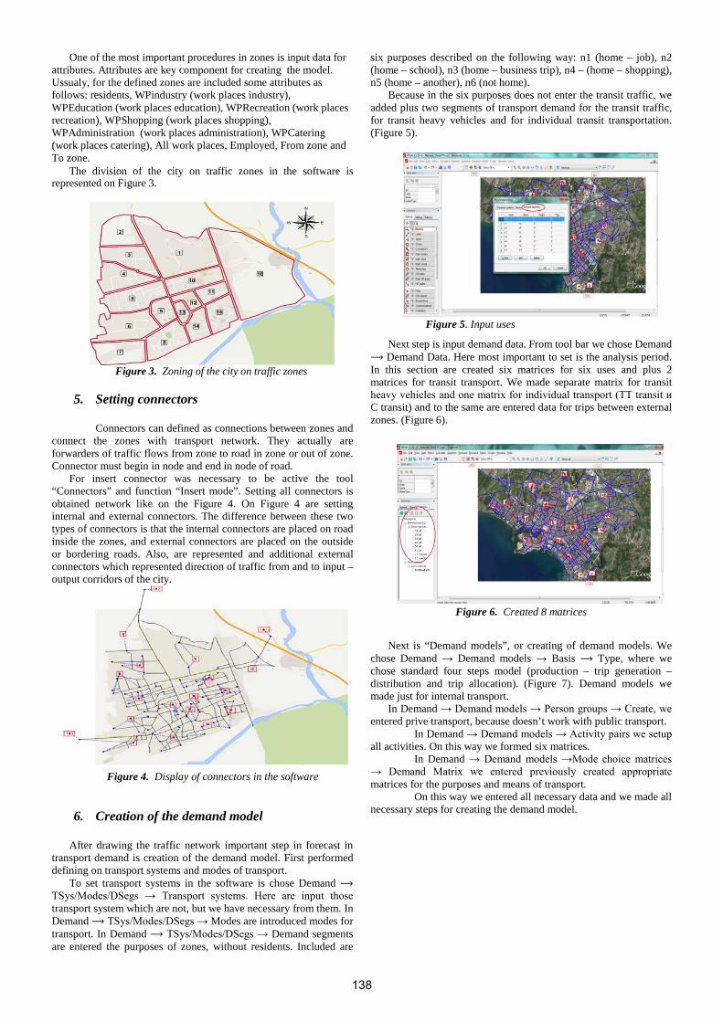
One of the most important procedures in zones is input data for attributes. Attributes are key component for creating the model. Ussualy, for the defined zones are included some attributes as follows: residents, WPindustry (work places industry), WPEducation (work places education), WPRecreation (work places recreation), WPShopping (work places shopping), WPAdministration (work places administration), WPCatering (work places catering), All work places, Employed, From zone and To zone.

The division of the city on traffic zones in the software is represented on Figure 3.

Figure 3. Zoning of the city on traffic zones

5. Setting connectors

Connectors can defined as connections between zones and

connect the zones with transport network. They actually are forwarders of traffic flows from zone to road in zone or out of zone. Connector must begin in node and end in node of road.

For insert connector was necessary to be active the tool “Connectors” and function “Insert mode”. Setting all connectors is obtained network like on the Figure 4. On Figure 4 are setting internal and external connectors. The difference between these two types of connectors is that the internal connectors are placed on road inside the zones, and external connectors are placed on the outside or bordering roads. Also, are represented and additional external connectors which represented direction of traffic from and to input – output corridors of the city.

Figure 4. Display of connectors in the software

6. Creation of the demand model

After drawing the traffic network important step in forecast in

transport demand is creation of the demand model. First performed defining on transport systems and modes of transport.

To set transport systems in the software is chose Demand ⟶ TSys/Modes/DSegs → Transport systems. Here are input those transport system which are not, but we have necessary from them. In Demand ⟶ TSys/Modes/DSegs → Modes are introduced modes for transport. In Demand ⟶ TSys/Modes/DSegs → Demand segments are entered the purposes of zones, without residents. Included are

six purposes described on the following way: n1 (home – job), n2 (home – school), n3 (home – business trip), n4 – (home – shopping), n5 (home – another), n6 (not home).

Because in the six purposes does not enter the transit traffic, we added plus two segments of transport demand for the transit traffic, for transit heavy vehicles and for individual transit transportation. (Figure 5).

Figure 5. Input uses

Next step is input demand data. From tool bar we chose Demand ⟶ Demand Data. Here most important to set is the analysis period. In this section are created six matrices for six uses and plus 2 matrices for transit transport. We made separate matrix for transit heavy vehicles and one matrix for individual transport (TT transit и C transit) and to the same are entered data for trips between external zones. (Figure 6).

Figure 6. Created 8 matrices

Next is “Demand models”, or creating of demand models. We

chose Demand → Demand models → Basis ⟶ Type, where we chose standard four steps model (production – trip generation – distribution and trip allocation). (Figure 7). Demand models we made just for internal transport.

In Demand → Demand models → Person groups → Create, we entered prive transport, because doesn’t work with public transport.

In Demand → Demand models → Activity pairs we setup all activities. On this way we formed six matrices.

In Demand → Demand models →Mode choice matrices → Demand Matrix we entered previously created appropriate matrices for the purposes and means of transport.

On this way we entered all necessary data and we made all necessary steps for creating the demand model.

138

Figure 7. Standard four step model

7. Procedures for calculation on transport

demand

Procedures for calculation on transport demand are most important part for the model. Here are made trip generation, trip distribution and trip assignment. In the concrete example we does not inspected modal split, because we don’t have data for public transport.

Procedures for calculation began with choosing the commands Calculate ⟶ Procedures → Operations. Here we made trip distribution and generation for all purposes. Trip generation we made on this way: Calculate ⟶ Procedures → Operations → Create group. On this way we made six groups for all six groups of activities. Click on any of the groups in “Demand model” we chose “Trip generation” and we clicked “Ok”. On this way we entered trip generations for which are entered appropriate factors for attraction and production for each activity for which we have factors, in depends of the purposes.

Figure 8 represented entered factors for production and attraction.

Figure 8. Trip generation and entered factors

In the same way as we made trip generation we made and trip

distribution. But, before we created Skim matrix, which is matrix of resistance of trips. This matrix we created choosing the following commands: Calculate ⟶ Procedures ⟶ Operations ⟶ Create → Matrices ⟶ Calculate ⟶ PrT skim matrix →Ok. We defined their parameters and demand segments and calculated using the tool “Execute” in Procedures ⟶ Operations so that preclude generation and production, with unselected in Active. (Figure 9).

Figure 9. Display on Skim matrix

Further we created distribution, in the same way as the trip

generation. How much we have generation, we have so and distribution. Also, in distribution are included appropriate factor for distribution.

Figure 10 represented the way of creating the distribution.

Figure 10. Creating distribution

In this section left to enter the assignment (PrT

Assignment) on private transport. This is made choosing the next commands: Calculate ⟶ Procedures ⟶ Operations ⟶ Create → Assignment ⟶ PrT Assignment ⟶ Ок.

Photo 11 represented the way of entered the assignment on private transport.

Figure 11. Assignment on private transport

In Calculate ⟶ Procedures ⟶ Operations → Selection DSeg.,

we selected all demand segments, and in “Procedure” we choose “Equilibrium assignment”.

In Calculate ⟶ Procedures ⟶ Operations → Parameters → OD demand share per iteration step we take itaration in tre steps, in the first step we write 34, at 2 – 33, at 3 – 33 and we activated Ок. (Figure 12).

139

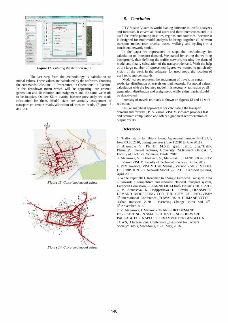
Figure 12. Entering the iteration steps

The last step from the methodology is calculation on modal values. These values are calculated by the software, choosing the commands Calculate ⟶ Procedures ⟶ Operations ⟶ Execute. In the dropdown menu which will be appearing, are entered generation and distribution and assignment and the same we made to be inactive. Outlaw Skim matrix, because previously we made calculation for them. Modal sizes are actually assignment of transport on certain roads, allocation of trips on roads, (Figure 13 and 14).

Figure 13. Calculated modal values

Figure 14. Calculated modal values

8. Conclution

PTV Vision Visum is world leading software in traffic analyzes and forecasts. It covers all road users and their interactions and it is used for traffic planning in cities, regions and countries. Because it is designed for multimodal analysis he brings together all relevant transport modes (car, trucks, buses, walking and cycling) in a consistent network model.

In the paper we represented in steps the methodology for calculation on transport demand. We started by setting the working background, than defining the traffic network, creating the demand model and finally calculation of the transport demand. With the help of the large number of represented figures we wanted to get clearly vision of the work in the software, for used steps, the location of used tools and commands.

Modal values represent the assignment of travels on certain roads, i.e. distribution on travels on road network. For modal values calculation with the fourstep model, it is necesarry activation of all generation, distribution and assignment, while Skim matrix should be deactivated.

Intensity of travels on roads is shown on figures 13 and 14 with red color.

Unlike analytical approaches for calculating the transport demand and forecast , PTV Vision VISUM software provides fast and accurate computation and offers a graphical representation of output results.

References

1. Traffic study for Bitola town, Agreement number 08-1124/1, from 03.06.2010, during one year (June 1 2010 to June 2011). 2. Atanasova V., Ph. D., M.S.E., grad. traffic. Eng."Traffic Planning", internal lectures, University "St.Kliment Ohridski ", Faculty of Technical Sciences, Bitola, 2010. 3. Atanasova, V., Detelbach, S., Markovik, l., HANDBOOK PTV

Vision VISUM, Faculty of Technical Sciences, Bitola, 2012 4. PTV America, VISUM User Manual, Version 7.50. 2. MODEL DESCRlPTlON. 2.1. Network Model. 2-3. 2.1.1. Transport systems, April 2001. 5. White Paper 2011, Roadmap to a Single European Transport Area – Towards a competitive and resource efficient transport system, European Comission, - COM/2011/0144 final/ Brussels, 28.03.2011. 6. V. Atanasova, K. Hadjipetkova, D. Ilievski ,,TRANSPORT DEMAND MODELLING FOR THE CITY OF RADOVISH“ 5th International Conference ,,TOWARDS A HUMANE CITY“ – Urban transport 2030 - Mastering Change Novi Sad, 5th - 6th November 2015 7. V. Atanasova, L.Markovik TRANSPORT DEMAND FORECASTING IN SMALL CITIES USING SOFTWARE PACKAGE FOR A SPECIFIC EXAMPLE FOR GEVGELIJA TOWN, I International Conference ,,Transport for Today’s Society” Bitola, Macedonia, 19-21 May, 2016

140

DRY SLIDING WEAR PROPERTIES OF Al(4%Cu) - SiC COMPOSITES WITHOUT AGE HARDENING

A. Kazaz1, H. Erdem Çamurlu2, M. Ayşe Dere2

Akdeniz University, Faculty of Engineering, Civil Engineering Department, 07058 Antalya, Turkey 1

Akdeniz University, Faculty of Engineering, Mechanical Engineering Department, 07058 Antalya, Turkey 2

erdemcamurlu@gmail.com

Abstract: Dry sliding wear behaviour of unreinforced Al4%Cu and Al4%Cu - SiC composites was investigated. Composites containing 10-50 vol. % SiC were obtained via hot press by using Al, Cu and SiC starting powders. Wear tests were conducted by an oscillating tribometer having a 6 mm diameter alumina ball. 2 N load was employed and sliding span was 5 mm with a total test distance of 6 m. Wear tracks were examined by an optical microscope, track cross sectional areas were determined by a profilometer and wear rates were calculated. It was seen that the wear track formed on the unreinforced sample was much larger and deeper than the ones on the composite samples. Wear mechanism was suggested to be initially adhesive and then adhesive and abrasive. The wear rate of unreinforced sample was about 11x10-3 mm3/N.m. Wear rate was seen to decrease abruptly with the addition of SiC particles into the matrix alloy. When 10 vol. % SiC was used, wear rate decreased to 1.5x10-3 mm3/N.m. The lowest wear rate was achieved in the sample containing 30 vol. % SiC, 0.5x10-3 mm3/N.m.

Keywords: Dry sliding wear, SiC reinforced aluminum matrix composite, Powder metallurgy

1. Introduction The incorporation of hard ceramic particles such as SiC, B4C,

TiB2, Al2O3 has been utilized in order to enhance hardness and wear resistance of light alloys such as aluminum, etc. [1-6]. The properties such as hardness, toughness and wear resistance of the formed material, which is technologically termed as ceramic particle reinforced metal matrix composite, can be altered by varying the particulate size or content and the properties of the matrix alloy.

Particulate reinforced light metal matrix composite materials are especially suitable where weight of the part is important, due to their lightweight. These materials can be used in applications like aircraft structural and wear parts as well as in automotive industry, such as pistons, brake components, etc., with the aim of weight reduction [7]. Sliding wear resistance is important for tribological applications requiring high performance [6].

Wear resistance of aluminum matrix composites which were produced by various techniques such as stir casting, extrusion, etc. and reinforced with hard ceramic particles, have been investigated [4-7]. The common outcome of these studies, regardless of the employed production method is that, the incorporation of the hard ceramic particles enhances wear resistance, as compared to unreinforced alloy and that wear resistance generally increases with the increase in the amount of the reinforcement particles [4-6]. In these studies, in order to determine the sliding wear characteristics, a pin on disc testing apparatus is commonly utilized [4-6,8] with various loads and for various distances of wear tests. In the study of Rao et al. [4], SiC reinforced Al MMCs were produced by stir casting. It was reported that the wear resistance of the composites depends to a large extent on the matrix alloy, where AA2024 was found to possess the best wear resistance. In the study of Alpas et al. [6], SiC reinforced Al MMCs were obtained as produced commercially. Shirazi et al. obtained the SiC-Al6061 composites through hot extrusion at 500 oC [5]. It was seen that when SiC particles of 25-50 nm size were used, low amounts such as 1-3 wt.% of SiC was sufficient to enhance hardness and wear resistance of the Al MMCs [5].

Aluminum alloys reinforced with hard ceramic particles have the potential to be used in applications where wear resistance is required. Therefore, estimation of their sliding wear properties is of technological interest. SiC particle reinforced Al (4%Cu) metal matrix composites were produced via hot pressing method [9] and their sliding wear characteristics were determined in the present study.

2. Experimental Procedure Composite samples, which were subjected to wear tests, were

produced by hot pressing of mixed elemental aluminum (Merck), elemental copper (Alfa Aesar) and SiC (Alfa Aesar) powders at 550 oC for 30 min. The SiC amounts were adjusted so that the composites contained 10 – 50 vol.% SiC, with 10 vol.% increments.

Hardness values of the composites were determined by using a Brinell hardness tester (HB10). Wear tests of the composites were conducted with an oscillating (reciprocally sliding) tribometer (Tribotechnic) according to DIN 50324 Standard (Testing Of Friction And Wear Model Test For Sliding Friction Of Solids (Ball-On-Disc System)). A 6 mm diameter alumina ball was used for wearing the composites under 2 N load. The span length was 5 mm and 6 m of total test distance was employed for each specimen. The test was stopped after 2 m and 1 m intervals and the profile of the wear track was determined by using a profilometer (rugosimeter, (Taylor Hobson, Surtronik 25)). The area of the wear track cross section was multiplied by the span length (5 mm) in order to calculate the wear track volume. Wear rate (mm3/N.m) was calculated via dividing the wear track volume by the applied load (2 N) and test distance.

3. Results and Discussion Wear tracks formed on the unreinforced alloy and on the SiC

particle containing composites are presented in Fig. 1. These tracks were formed as a result of the repeated sliding contact of alumina ball, which was used as the counter body. Detached flakes of wear debris were seen around the wear tracks of all the specimens, especially at the ends of the tracks. It can be seen that when no reinforcement SiC particles were used the wear track was quite large, about 960 microns. Wear track width was seen to decrease with the increase in the amount of SiC particles in the Al4%Cu matrix. There was an abrupt decrease when 10 vol. % SiC was added into the matrix. In the composite containing 50 vol. % SiC, wear track width was about 330 microns.

In the wear track of the unreinforced Al4%Cu matrix alloy (Fig. 1a), continuous grooves were seen to form along the sliding direction. Unreinforced matrix had the lowest hardness and highest ductility, among the studied samples [9]. There are patches of smeared particles inside the wear track of this sample. Due to the repeated stress under the alumina ball, work hardening occurs on the aluminum surface and this results in the detachment of the debris. The ductile wear debris, torn and detached from the surface of the sample, may have stuck or attached back into the wear track

141

and formed patches of smeared debris inside the track. It is expected that initially adhesive wear mechanism is dominant and later abrasive wear mechanism takes place. Initial sticking of the aluminum matrix and alumina ball results in the initial adhesive wear. The aluminum particles attached on the surface of the alumina ball is expected to cause abrasive wear on the work hardened aluminum surface. This takes place by the tearing of the aluminum along the sliding direction.

The continuous wear grooves on the wear tracks of the composite samples (Fig. 1b-d) were seen to become thinner with the increase in the amount of SiC particles. In addition, patches of smeared ductile particles were not present and inside of the wear tracks were smoother.

Fig. 1 Optical micrographs of the wear tracks on the (a) unreinforced Al4%Cu matrix alloy, (b) 10, (c) 30, (d) 50 vol. % SiC containing composites.

Wear track width alone is not sufficient to quantify the wear amount or rate, since for that, depth of the wear track is also necessary. Therefore, wear track profiles were determined by using a profilometer. Wear track profiles of unreinforced sample and of composite containing 40% SiC are presented in Fig. 2. It can be seen that the inner surface of the wear track of unreinforced sample is not smooth, but contains grooves. The presence of the re-attached soft wear debris on the inner surface of the wear track renders the wear track surface irregular and rough. The maximum depth of this wear track was about 40 microns, with a width of about 1 mm. The width of the track is consistent with the measurements made on optical micrographs (Fig.1a). Cross sectional area of the wear track was about 20000 square microns. Volumes of the wear tracks were calculated via multiplying the cross sectional area by the length of the wear track (5 mm).

The wear track width of the composite containing 40 % SiC was about 0.4 mm and the maximum depth was about 6 microns. Cross sectional area of the wear track was about 1600 square microns. It can be seen that the presence of SiC particles in aluminum matrix reduces wear and increases wear resistance.

Fig. 2 Wear track profile formed on (a) unreinforced sample and on (b) 40 % SiC containing composite. (note the change in the scales)

(a)

(b)

(c)

(d)

(a)

(b)

142

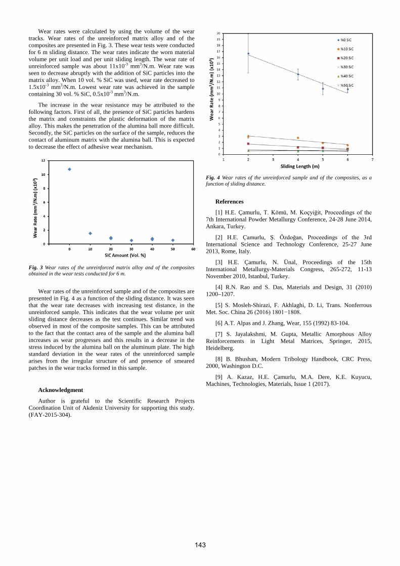
Wear rates were calculated by using the volume of the wear tracks. Wear rates of the unreinforced matrix alloy and of the composites are presented in Fig. 3. These wear tests were conducted for 6 m sliding distance. The wear rates indicate the worn material volume per unit load and per unit sliding length. The wear rate of unreinforced sample was about 11x10-3 mm3/N.m. Wear rate was seen to decrease abruptly with the addition of SiC particles into the matrix alloy. When 10 vol. % SiC was used, wear rate decreased to 1.5x10-3 mm3/N.m. Lowest wear rate was achieved in the sample containing 30 vol. % SiC, 0.5x10-3 mm3/N.m.

The increase in the wear resistance may be attributed to the following factors. First of all, the presence of SiC particles hardens the matrix and constraints the plastic deformation of the matrix alloy. This makes the penetration of the alumina ball more difficult. Secondly, the SiC particles on the surface of the sample, reduces the contact of aluminum matrix with the alumina ball. This is expected to decrease the effect of adhesive wear mechanism.

Fig. 3 Wear rates of the unreinforced matrix alloy and of the composites obtained in the wear tests conducted for 6 m.

Wear rates of the unreinforced sample and of the composites are presented in Fig. 4 as a function of the sliding distance. It was seen that the wear rate decreases with increasing test distance, in the unreinforced sample. This indicates that the wear volume per unit sliding distance decreases as the test continues. Similar trend was observed in most of the composite samples. This can be attributed to the fact that the contact area of the sample and the alumina ball increases as wear progresses and this results in a decrease in the stress induced by the alumina ball on the aluminum plate. The high standard deviation in the wear rates of the unreinforced sample arises from the irregular structure of and presence of smeared patches in the wear tracks formed in this sample.

Acknowledgment

Author is grateful to the Scientific Research Projects Coordination Unit of Akdeniz University for supporting this study. (FAY-2015-304).

Fig. 4 Wear rates of the unreinforced sample and of the composites, as a function of sliding distance.

References

[1] H.E. Çamurlu, T. Kömü, M. Koçyiğit, Proceedings of the 7th International Powder Metallurgy Conference, 24-28 June 2014, Ankara, Turkey.

[2] H.E. Çamurlu, Ş. Özdoğan, Proceedings of the 3rd International Science and Technology Conference, 25-27 June 2013, Rome, Italy.

[3] H.E. Çamurlu, N. Ünal, Proceedings of the 15th International Metallurgy-Materials Congress, 265-272, 11-13 November 2010, Istanbul, Turkey.

[4] R.N. Rao and S. Das, Materials and Design, 31 (2010) 1200–1207.

[5] S. Mosleh-Shirazi, F. Akhlaghi, D. Li, Trans. Nonferrous Met. Soc. China 26 (2016) 1801−1808.

[6] A.T. Alpas and J. Zhang, Wear, 155 (1992) 83-104.

[7] S. Jayalakshmi, M. Gupta, Metallic Amorphous Alloy Reinforcements in Light Metal Matrices, Springer, 2015, Heidelberg.

[8] B. Bhushan, Modern Tribology Handbook, CRC Press, 2000, Washington D.C.

[9] A. Kazaz, H.E. Çamurlu, M.A. Dere, K.E. Kuyucu, Machines, Technologies, Materials, Issue 1 (2017).

143

MECHANICAL CHARACTERIZATION OF RECYCLED POLYPROPYLENE AND COPOLYMER MACRO FIBERS IN CONCRETE

Mehmet Alpaslan KÖROĞLU

1Necmettin Erbakan University, Engineering & Architectural Faculty, Konya, TURKEY makoroglu@konya.edu.tr

Abstract: Waste materials have been an increasing problem every year. Disposal of waste materials has presented very serious problems to the human community in the world. Currently, some research has been studied to the recycle of different wastes in concrete. Recent study is focusing on the usage of a unique blend of recycled polypropylene and copolymer macro fibers (RPCMF) designed specifically for concrete mixture. The different weight of RPCMF is mixed in concrete to in order to investigate the effect on mechanical properties. By adding RPCMF obtained a satisfactory improvement on cracking control, compressive strength, flexural strength and also tensile strength, Moreover, compressive, flexural and tensile strength was positively affected by the addition of RPCMF for some mixtures. More percentage of weight fractions added gives high result in tensile strength. However, the workability of the concrete reinforced with RPCMF was negatively affected.

Keywords: Recycled Polypropylene, Copolymer Macro fiber, concrete, compressive strength, flexural strength

1. Introduction Polypropylene (PP) fibers have been widely used to reinforce

concrete as an alternative to steel fibers. The reinforcing effect of the PP fiber is directly proportional to its tensile strength and Young modulus. Polypropylene fibers have been widely used in concrete, plaster, mortar, and shotcrete applications nowadays. The additions of these fibers to concrete considerably improve the structural characteristics of concrete such as flexural strength, impact strength, tensile strength, ductility and toughness [1].

Polypropylene fibers are manufactured in different size and shape, and with various properties which are hair-like or made of plastic with the chemical structure containing a long chain of individual molecules.

PP fibers are manufactured with three different geometrics. Monofilaments, film and extruded tape are the typical PP geometries which the last two forms are used widely for concrete reinforcement [2]. The PP has a high melting point (165°C), alkali resistance and low cost of raw material but has a low tensile strength [2]. And also, since it is hydrophobic material, water absorption of pp is zero that leads preventing adhesion to the concrete [3]. However, PP has some weakness points such as: sensitivity to oxygen and sunlight, poor fire resistance, low modulus of elasticity and poor bond with the matrix [2].

The objective of the current research is to study the mechanical properties of concrete reinforced individually with weight percentage of with 0.125, 0.25, 0.5 % of RPCMF to evaluate their strength.

2. Materials and Method Recycled polypropylene and copolymer macro fibers (RPCMF)

is a unique blend of recycled polypropylene and copolymer macro fibers produced for concrete applications that consists of 100% recycled polypropylene fibrillated (network) fibers and a high-performance twisted-bundle macro-monofilament fiber. The specific gravity of RPCMF is 0,9 and has the tensile strength of 570 MPa. 58 mm length RPCMF is used in this study (Figure 1).

Fig. 1 Recycled polypropylene and copolymer macro fibers

Following materials utilized in the present research:

Ordinary Portland cement according to TS EN 197-1, CEM I 32.5 R cement was used for every concrete mixture. Raw materials used in this research include cement, fine aggregate (natural river sand), coarse aggregate and fibers. Natural river sand with a maximum size of 5 mm, specific gravity of 1.52, SSD water absorption of 1.37%, and SSD density of 2512 kg/m3 was used in this study. Course aggregate with a max a maximum aggregate size of 15 mm was used. Specific weight of course aggregate is found as 2690 kg/m3 and SSD water absorption of 0.6 %. Both natural river sand and course aggregates were batched in a dry condition.

For preparation of all the samples, a water–cement ratio (w/c) of 0.55 (by weight) was used. Table 1 represents the details of the mixture proportions.

Table 1. Concrete mix design

Fine Aggregate

Course Aggregate Cement Water

Weight Percent

Sample (gr) (gr) (gr) (gr) (%)

Reference 18090 22110 9900 5400 0

0,125% 18090 22110 9900 5400 0,125

0,25% 18090 22110 9900 5400 0,25

0,5% 18090 22110 9900 5400 0,5

All standard steel moulds for cubes, cylinders and prisms specimens has been prepared by oiling the inner surface of the formwork before casting in order to remove the mould after the concrete hardened.

Concrete mixing process was performed to ensure that steel fibers were distributed uniformly in the concrete mix. In the first stage, all ingredients (cement, fine aggregate, water and course aggregate) were mixed well then after steel fibers are added gradually.

2.2. Slump Test

In order to obtain workability of fresh concrete mixture slump test is applied to all mixtures (Figure 2). Slump height for the control specimen which is plain concrete is 90 mm. Slump height was decreased since the addition of fiber into concrete mixture. From 0.125% until 0.5%, the slump height was decreasing. Slump height is calculated to be 70 mm for 0.125% of fiber weight, 45 mm for 0.25% of fiber weight and 20 mm for 0.5% of fiber weight. It is indicates that the slump of the mixture was decreased when the RPCMF content increased.

144

Fig. 2 Slump test

The compressive strength test for the cubes was applied at the ages of 28 days. A total of 18 concrete cubes with the dimensions of 150×150×150mm were prepared. 3 specimens were prepared for each percentage weight fraction of RPCMF (0.0%, 0.125 %, 0.25%, 0.5 %). ASTM C 109 is use to determine compressive strength for the concrete that is used in this study (Figure 3.).

Fig. 3. Compressive strength test

A total of 3 prismatic specimens with the overall dimensions of 150×150×400 mm were tested for each percentage weight fraction of RPCMF (0.0%, 0.125 %, 0.25%, 0.5 %). The 3 point flexure test was carried out at the age of 28 days with the standard of ASTM D790 (Figure 4.).

Fig 4 Beam specimen after 3 point flexure test

The results of split tensile strength test were based on cylinders with various weight fraction of tire fiber for 28th days. In the course of split tensile strength test, specimens were tested by applying an increasing load throughout the vertical diameter until split failure occurs. Failure of the specimens comes of along its vertical diameter, owing to tension developed in the transverse direction.

3. Results The concrete properties with different weight fraction of

RPCMF are summarized in Table 2.

Table 2. Concrete properties with different weight fraction of RPCMF

Weight of

Fiber %

Slump (mm)

Unit Weight

(kg/m3)

Compressive Strength (MPa)

Flexural Strength (MPa)

Tensile Strength (MPa)

0 90 2210 25,05 2,99 2,36

0,125 70 2232 27,96 3,11 2,57

0,25 45 2239 30,68 4,29 2,64

0,5 20 2255 30,93 4,38 2,79

From Table 2. above, the highest average compressive strength is is at 0.25% which is 30.68 MPa of fiber weight whereas the lowest strength is at 0% which is 28.05 MPa. Although stress for 0.5% fiber weight sample is lower than 0.125% fiber weight sample, the strain is more. Figure 5. shows that increasing fiber content also increase ductility of the concrete under compression force. Increasing fiber content not only develop ductility of concrete but also compression strength.

Fig 5. Stress-strain diagram for RPCMF concrete

Result of tensile strength of the control cylinder is found to be 2.36 MPa and decrease until 2.57 MPa at 0.125% and increase again at 0.25% which is 2.64 MPa. It is seen from Table 2., the highest flexural strength is at 0.5% of fibre content which is 4.38 MPa and the lowest strength is at 0% of fibre volume which is 2.99 MPa.

4. Conclusions This research has proved that the performance of RPCMF

reinforced concrete is much better compare to conventional plain concrete. The conclusions from this research based on the experimental results are:

• The test result shows that as the fiber weight of fraction increase the workability tend to decrease significantly. Moreover, it can be realized that, the slump test decreases when the weight of fiber increases.

• RPCMF reinforced concrete may be used in order to increase the mechanical properties of concrete. High percentage of weight fraction gives high flexural strength of the concrete.

• The concrete with RPCMF absorb more energy before and after fail. The RPCMF in concrete grips the concrete particles when load is applied on it until failure.

• The crack opening width can be controlled by using RPCMF in concrete.

• Split tensile test and 3 point flexural test indicate that concrete reinforced with RPCMF has much greater toughness compared to plain concrete. The cylinder does not split during tensile test since the presence of RPCMF in concrete. Moreover, concrete prism also does not break into two because of the RPCMF reinforced in concrete.

References [1] Mohammadi, Yaghoub et al., “Properties of steel fibrous

concrete containing mixed fibers in fresh and hardened state”, Construction and Building Materials, (2008), 22 956–965. [3]

[2] Bentur, A. and S. Mindess, Fibre reinforced cementitious composites. 2005, England: Taylor & Francis e-Library.

[3] Commitee, A., State-of-the-Art Report on Fiber Reinforced Concrete (ACI 544.1R-96). 2001: American Concrete Institute.

145