sta 4210 supplementary notes and r programs
TRANSCRIPT

STA 4210 – Supplementary Notes and R Programs
Larry Winner
Department of Statistics
University Of Florida

Introduction/Review
Mathematical Operations – Summation Operators
Consider sequences of numbers and numeric constants.
1
1
1
1 1 1
Sum of a sequence of Variables: ...
Sum of a sequence of Constants: ...
Sum of a sequence of Sums of Variables:
Sum of a sequence of (Commonly) Li
n
i n
i
n
i
n n n
i i i i
i i i
Y Y Y
k k k nk
X Z X Z
1 1
1 1 1
nearly Transformed Variables:
Sum of a sequence of (Individually) Linearly Transformed Variables:
Sum of a sequence of Sums of Multiples of Variable
n n
i i
i i
n n n
i i i i i i
i i i
a bX na b X
a b X a b X
1 1 1
s: n n n
i i i i i i i i
i i i
a X b Z a X b Z
Example – Opening Weekend Box-Office Gross for Harry Potter Films
Date Movie Gross($M) Theaters PerTheater($K) Euros/Dollar Gross (€M)
11/16/2001 Sorcerer's Stone 90.29 3672 24.59 1.1336 102.36
11/15/2002 Chamber of Secrets 88.36 3682 24.00 0.9956 87.97
6/4/2004 Prisoner of Azkaban 93.69 3855 24.30 0.8135 76.21
11/18/2005 Goblet of Fire 102.69 3858 26.62 0.8496 87.24
7/13/2007 Order of the Phoenix 77.11 4285 18.00 0.7263 56.00
7/17/2009 Half-Blood Prince 77.84 4325 18.00 0.7085 55.15
11/19/2010 Deathly Hallows: Part I 125.02 4125 30.31 0.7353 91.93
7/15/2011 Deathly Hallows: Part II 169.19 4375 38.67 0.7042 119.14
Total 824.18 32,177.00 676.00
1
1
Total Gross ($Millions): 90.29 88.36 ... 169.19 824.18
Total Gross (Millions of Euros): 1.1336(90.29) 0.9956(88.36) ... 0.7042(169.19) 676.00
n
i
i
n
i i
i
Y
a Y
Question: What is the average gross per theater for all movies? Is it the same as the average of individual
movies per theater?
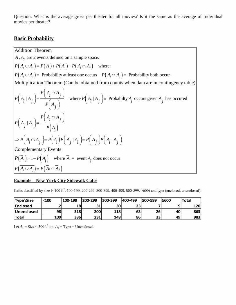
Basic Probability
Example – New York City Sidewalk Cafes Cafes classified by size (<100 ft
2, 100-199, 200-299, 300-399, 400-499, 500-599, ≥600) and type (enclosed, unenclosed).
Type\Size <100 100-199 200-299 300-399 400-499 500-599 ≥600 Total
Enclosed 2 18 31 30 23 7 9 120
Unenclosed 98 318 200 118 63 26 40 863
Total 100 336 231 148 86 33 49 983
Let A1 ≡ Size < 300ft2 and A2 ≡ Type = Unenclosed.
, are 2 events defined on a sample space.
where:
Probability at least one occurs Probability both occur
Addition Theorem
Multiplication Theorem (Can be obta
i j
i j i j i j
i j i j
A
P A P A P A P A
P A P A
A
A A
A A
| where | Probabilty occurs given has occured
|
|
ined from counts when data are in contingency table)
P A Ai j
P A A P A A A Ai j i j i j
P Aj
P A Ai j
P A Aj i
P Ai
P A A P A P Ai j i j
|
1 where event does not occur
Complementary Events
i i
i ji j
A P A P A Ai j i j
A P A A Ai i
P A P A A
P
A

1
2
1 2 1 2
1 2 1 2 1 2
1 2
1 2
2
100 336 231 6670.6785
983 983
8630.8779
983
98 318 200 6160.6267
983 983
667 863 616 9140.9298 0.6785 0.8779 0.6267
983 983
616 0.6267| 0.7138
863 0.87
P A
P A
P A A P A A
P A A P A P A P A A
P A AP A A
P A
1 2
2 1
1
1
2
1 2 1 2
79
616 0.6267| 0.9235
667 0.6785
148 86 33 49 3160.3215 1 0.6785
983 983
1200.1221 1 0.8779
983
30 23 7 9 690.0702
983 983
P A AP A A
P A
P A
P A
P A A P A A
Univariate Random Variables
1Discrete (RV takes on masses of probability at specific points ,..., ):
1,..., often written where is specific point
Continuous (RV take
Probability (Density) Functions
k
s s s
Y Y Y
f Y P Y Y s k f y y Y
Y
s on density of probability over ranges of points on continuum)
density at (confusing notation, often written where is specific point and is RV)
Expected Value (Long Run Average Outcome,
f Y Y f y y Y
1
22 2
Continuous:
, constants
aka Mean)
Discrete:
Variance (Average Squared Distance from Expected Value)
k
Y s s Y
s
Y Y
Y
Y Y f Y Y Yf Y dY yf y dy
a c E a cY a c Y a c E a a E cY c Y c
Y E Y Y E Y
E E
E E
E
2
22 2 2 2 2
2 2 2 2 2 2 2 2 2 2 2
Equivalently (Computationally easier):
, constants 0
Y
Y Y
Y Y
Y E Y Y E Y
a c a cY c Y c a cY c Y c
E

Example – Total Goals per Game in National Women’s Soccer League Games (2013)
Goals (y) Frequency Probability=p(y) y*p(y) (y^2)*p(y)
0 4 0.0455 0.0000 0.0000
1 16 0.1818 0.1818 0.1818
2 26 0.2955 0.5909 1.1818
3 20 0.2273 0.6818 2.0455
4 9 0.1023 0.4091 1.6364
5 6 0.0682 0.3409 1.7045
6 5 0.0568 0.3409 2.0455
7 2 0.0227 0.1591 1.1136
Total 88 1 2.7045 9.9091
0
0.05
0.1
0.15
0.2
0.25
0.3
0.35
0 1 2 3 4 5 6 7
P
r
o
b
a
b
i
l
i
t
y
Goals
Probability Distribution
Note: Using more common notation, where y represents a specific outcome (number of goals) and p(y) represents the probability of a
game having y goals
7
0
722 2 2 2 2 2 2
0
2
Expected Value (Mean): ( ) 0(.0455) ... 7(.0227) 2.7045
Variance: ( ) 9.9091 2.7045 2.5945
Standard Deviation: 2.5945 1.6108
Y
y
Y
y
Y
E Y yp y
Y E Y E Y y p y
Y Y

Bivariate Random Variables
Example – Goals by Half Y=Home Club Z=Away Club – Irish Premier League (2012)
H\A Freq 0 1 2 3 4 5 Total(Home)
0 105 67 20 8 0 0 200
1 75 41 18 1 0 0 135
2 26 17 1 0 1 0 45
3 6 3 3 0 0 0 12
4 1 1 0 0 0 0 2
5 2 0 0 0 0 0 2
Total(Away) 215 129 42 9 1 0 396
H\A Prob 0 1 2 3 4 5 Total(Home)
0 0.26515 0.16919 0.05051 0.02020 0.00000 0.00000 0.50505
1 0.18939 0.10354 0.04545 0.00253 0.00000 0.00000 0.34091
2 0.06566 0.04293 0.00253 0.00000 0.00253 0.00000 0.11364
3 0.01515 0.00758 0.00758 0.00000 0.00000 0.00000 0.03030
4 0.00253 0.00253 0.00000 0.00000 0.00000 0.00000 0.00505
5 0.00505 0.00000 0.00000 0.00000 0.00000 0.00000 0.00505
Total(Away) 0.54293 0.32576 0.10606 0.02273 0.00253 0.00000 1.00000
Random Variables (Outcomes observed on same unit) , ( possibilities for , for ) :
, 1,...
Joint Probability Function - Discrete Case (Generalizes to Densities in Continuous Case)
s t s t
Y Z k Y m Z
g Y Z P Y Y Z Z s
1
, ; 1,..., Probability and
Often written as , for specific outcomes ,
, Probabi
Marginal Probability Function - Discrete Case (Generalizes to Densities in Continuous Case):
s t
m
s s t
t
k t m Y Y Z Z
g y z y z
f Y g Y Z
1
lity , Probability Often denoted ( ), ( )
Continuous: Replace summations with integrals
Conditional Probability Function - Discrete Case (Generalizes to Densities in Conti
k
s t s t t
s
Y Y h Z g Y Z Z Z f y h z
,| 0; 1,..., Probability given Often denoted |
,| 0; 1,..., Probability given Often denoted h |
nuous Case) :
s t
s t t s t
t
s t
t s s t s
s
g Y Zf Y Z h Z s k Y Y Z Z f y z
h Z
g Y Zh Z Y f Y t m Z Z Y Y z y
f Y
Home Team
Distribution: f(y)
Away Team Distribution: g(z)

To obtain the conditional distribution of Away goals given a particular number of Home Goals, take the cell probabilities and divide
by the total row probability. Similarly, for the conditional distribution of Home goals given Away goals, divide cell by column total.
Conditional Distribution of Home goals given Away Goals=0 ≡ f(y|z=0):
0.26515 0.18939 0.065660 | 0 0.48837 1| 0 0.34884 2 | 0 0.12093
0.54293 0.54293 0.54293
0.01515 0.00253 0.005053 | 0 0.02791 4 | 0 0.00465 5 | 0 0.00930
0.54293 0.54293 0.54293
Note: 0.48837
f y z f y z f y z
f y z f y z f y z
0.34884 0.12093 0.02791 0.00465 0.00930 1
Covariance, Correlation, and Independence
2 2 2
2 2 2
Average Home Goals per Half: 0(0.50505) ... 5(.00505) 0.70455
Average Away Goals per Half: 0(0.54293) ... 5(.00000) 0.61616
0 (0.50505) ... 5 (.00505) 1.27525
0 (0.54293) ... 5 (.00000) 0.9
Y
Z
E Y
E Z
2 2
2 2
9495
0(0)(0.26515) 0(1)(0.16919) ... 5(5)(0.00000) 0.39647
1.27525 0.70455 0.77887 0.77887 0.88254
0.99495 0.61616 0.61529 0.61529 0.78441
, 0.39647 0.70455(0.61616) 0.0
Y Y
Z Z
YZ Y Z
E YZ
Y Z E YZ
3765
0.037650.05439
0.88254(0.78441)
YZYZ
Y Z
1 1
,
Equivalently (for computing): ,
Note: Discrete: , (Replace summati
Covariance - Average of Product of Distances from Means
YZ Y Z
YZ Y Z
k m
s t s t
s t
Y Z E Y E Y Z E Z E Y Z
Y Z E YZ E Y E Z E YZ
E YZ Y Z g Y Z
1 1 2 2 1 1 2 2 1 2 1 2
1 2 1 2 1 2 1 2
ons with integrals in continuous case)
, , , are constants , ,
, , , ,
Correlation: Covariance scaled to lie between -1 and +1 f
YZ
YZ YZ
a c a c a c Y a c Z c c c c Y Z
c Y c Z c c c c Y Z a Y a Z Y Z
Standardized Random Variables (Scaled to have mean=0, variance=1) '
,, ', ' 1 , 1
, , 0 , are uncorrelated (not necessarily
or measure of association strength
Y
Y
YZ
Y E Y YY
Y
Y ZY Z Y Z Y Z
Y Z
Y Z Y Z Y Z
independent)
, are independent if and only if , 1,..., ; 1,...,
If , are jointly normally distributed and , 0 then , are independent
Independent Random Variables
s t s tY Z g Y Z f Y h Z s k t m
Y Z Y Z Y Z

To see that Home and Away Goals are NOT independent (besides simply observing the correlation is not zero), you can check
whether the joint probabilities in the cells of the joint distribution are all equal to the product of their row and column totals (product
of the marginal probabilities).
For the case where both Home and Away goals are 0:
( 0, 0) 0.26515 ( 0) 0.50505 0 0.54293
0.26515 0.50505(0.54293) 0.27421
g y z f y h z
Linear Functions of Random Variables
Total Goals, Difference (Home – Away), and Average Goals by Half Y1 = Home Y2 = Away:
1
2 2 2 2
1 2 1 2 12
1 1 2 1 2
2 1 2 1 2
1 23 1 2
1 2
0.70455 0.61616 0.77887 0.61529 0.03765
Total Goals: 1, 1
Difference in Goals: 1, 1
1 1Average Goals: ,
2 2 2
1 1 1(0.70
Y Z Y Z YZ
U
U Y Y a a
U Y Y a a
Y YU a a
1
2
2
2 2 2 2 2
1 2 12
1 2
2 2 2 2 2
1 2 12
455) 1(0.61616) 1.32071
1 1 2(1)(1) 1(0.77887) 1(0.61529) 2( 0.03765) 1.31886
1 ( 1) 1(0.70455) 1(0.61616) 0.08838
1 ( 1) 2(1)( 1) 1(0.77887) 1(0.61529) 2( 0.03765
U
U
U
3
3
1 2
2 2
2 2 2
1 2 12
) 1.469461
1 1 1 1(0.70455) (0.61616) 0.66035
2 2 2 2
1 1 1 1 1 1 12 (0.77887) (0.61529) ( 0.03765) 0.32972
2 2 2 2 4 4 2
U
U
1
2 2
1 1 1
12 2 2 2
1 1 1 1 1 1
1 1 2 2 1
constants random variables
,
2
2
n
i i i i
i
i i i i i j ij
n n n
i i i i i i
i i i
n n n n n n
i i i j ij i i i j ij
i i j i i j i
U a Y a Y
E Y Y Y Y
E U E a Y a E Y a
U a Y a a a a a
n E a Y a Y a E
1 2 2 1 1 2 2
2 2 2 2 2 2 2 2 2
1 1 2 2 1 1 2 2 1 2 1 2 1 1 2 2 1 2 122 , 2
Y a E Y a a
a Y a Y a Y a Y a a Y Y a a a a

Linear Functions of INDEPENDENT Random Variables
Note: These do not apply for the soccer data, but are used repeatedly to obtain properties of estimators in linear
models.
Central Limit Theorem
When random samples of size n are selected from any population with mean m and finite variance s
2, the
sampling distribution of the sample mean will be approximately normally distributed for large n:
Z-table (and software packages) can be used to approximate probabilities of ranges of values for sample means,
as well as percentiles of their sampling distribution
2 2 2 2
1
1 1
1 2
2 2 2 2 2 2 2 2
1 1 2 1 1 2 1 2 1 2
2 2 2 2 2 2 2 2
2 1 2 2 1 2 1 2 1 2
1
,..., independent
Special Cases , independent :
(1) (1)
(1) ( 1)
,..., independent
n n
n i i i i
i i
n
Y Y U a Y a
Y Y
U Y Y U Y Y
U Y Y U Y Y
Y Y
2 2
1 1 1
1 2
2 2 2 2
1 2 1 2 1 2 1 2 1 2
,
Special Case , independent :
, , (1)(1) (1)( 1)
n n n
i i i i i i i
i i i
a Y c Y a c
Y Y
U U Y Y Y Y
2
1
1
1~ ,
approximately, for large
n
i ni
i
i
Y
Y Y Nn n n
n

Probability Distributions Widely Used in Linear Models
Normal (Gaussian) Distribution
• Bell-shaped distribution with tendency for individuals to clump around the group median/mean
• Used to model many biological phenomena
• Many estimators have approximate normal sampling distributions (see Central Limit Theorem)
• Notation: Y~N(,2) where is mean and
2 is variance
Probabilities can be obtained from software packages (e.g. EXCEL, R, SPSS, SAS, STATA). Tables can be
used to obtain probabilities once values have been standardized to have mean 0, and standard deviation 1.
2 2~ , ~ 0, 1YY Y Z Z
Y
YY N Z N
2
2
1 1 ( )exp , , 0
22
yf y y
0
0.005
0.01
0.015
0.02
0.025
0.03
0.035
0.04
0.045
0 20 40 60 80 100 120 140 160 180 200
f(y)
y
Normal Densities
N(100,400)
N(100,100)
N(100,900)
N(75,400)
N(125,400)
EXCEL Commands for Probabilities and Quantiles (Default are lower tail areas):
Lower tail (cumulative) probabilities: =norm.dist(y,mu,sigma,True)
Upper tail probabilities: =1 - norm.dist(y,mu,sigma,True)
pth
quantile: =norm.inv(p,mu,sigma) 0<p<1

Second Decimal Place of Z
F(z) 0.00 0.01 0.02 0.03 0.04 0.05 0.06 0.07 0.08 0.09
0.0 0.5000 0.5040 0.5080 0.5120 0.5160 0.5199 0.5239 0.5279 0.5319 0.5359
0.1 0.5398 0.5438 0.5478 0.5517 0.5557 0.5596 0.5636 0.5675 0.5714 0.5753
0.2 0.5793 0.5832 0.5871 0.5910 0.5948 0.5987 0.6026 0.6064 0.6103 0.6141
0.3 0.6179 0.6217 0.6255 0.6293 0.6331 0.6368 0.6406 0.6443 0.6480 0.6517
0.4 0.6554 0.6591 0.6628 0.6664 0.6700 0.6736 0.6772 0.6808 0.6844 0.6879
0.5 0.6915 0.6950 0.6985 0.7019 0.7054 0.7088 0.7123 0.7157 0.7190 0.7224
0.6 0.7257 0.7291 0.7324 0.7357 0.7389 0.7422 0.7454 0.7486 0.7517 0.7549
0.7 0.7580 0.7611 0.7642 0.7673 0.7704 0.7734 0.7764 0.7794 0.7823 0.7852
0.8 0.7881 0.7910 0.7939 0.7967 0.7995 0.8023 0.8051 0.8078 0.8106 0.8133
0.9 0.8159 0.8186 0.8212 0.8238 0.8264 0.8289 0.8315 0.8340 0.8365 0.8389
1.0 0.8413 0.8438 0.8461 0.8485 0.8508 0.8531 0.8554 0.8577 0.8599 0.8621
1.1 0.8643 0.8665 0.8686 0.8708 0.8729 0.8749 0.8770 0.8790 0.8810 0.8830
1.2 0.8849 0.8869 0.8888 0.8907 0.8925 0.8944 0.8962 0.8980 0.8997 0.9015
1.3 0.9032 0.9049 0.9066 0.9082 0.9099 0.9115 0.9131 0.9147 0.9162 0.9177
1.4 0.9192 0.9207 0.9222 0.9236 0.9251 0.9265 0.9279 0.9292 0.9306 0.9319
1.5 0.9332 0.9345 0.9357 0.9370 0.9382 0.9394 0.9406 0.9418 0.9429 0.9441
1.6 0.9452 0.9463 0.9474 0.9484 0.9495 0.9505 0.9515 0.9525 0.9535 0.9545
1.7 0.9554 0.9564 0.9573 0.9582 0.9591 0.9599 0.9608 0.9616 0.9625 0.9633
1.8 0.9641 0.9649 0.9656 0.9664 0.9671 0.9678 0.9686 0.9693 0.9699 0.9706
1.9 0.9713 0.9719 0.9726 0.9732 0.9738 0.9744 0.9750 0.9756 0.9761 0.9767
2.0 0.9772 0.9778 0.9783 0.9788 0.9793 0.9798 0.9803 0.9808 0.9812 0.9817
2.1 0.9821 0.9826 0.9830 0.9834 0.9838 0.9842 0.9846 0.9850 0.9854 0.9857
2.2 0.9861 0.9864 0.9868 0.9871 0.9875 0.9878 0.9881 0.9884 0.9887 0.9890
2.3 0.9893 0.9896 0.9898 0.9901 0.9904 0.9906 0.9909 0.9911 0.9913 0.9916
2.4 0.9918 0.9920 0.9922 0.9925 0.9927 0.9929 0.9931 0.9932 0.9934 0.9936
2.5 0.9938 0.9940 0.9941 0.9943 0.9945 0.9946 0.9948 0.9949 0.9951 0.9952
2.6 0.9953 0.9955 0.9956 0.9957 0.9959 0.9960 0.9961 0.9962 0.9963 0.9964
2.7 0.9965 0.9966 0.9967 0.9968 0.9969 0.9970 0.9971 0.9972 0.9973 0.9974
2.8 0.9974 0.9975 0.9976 0.9977 0.9977 0.9978 0.9979 0.9979 0.9980 0.9981
2.9 0.9981 0.9982 0.9982 0.9983 0.9984 0.9984 0.9985 0.9985 0.9986 0.9986
3.0 0.9987 0.9987 0.9987 0.9988 0.9988 0.9989 0.9989 0.9989 0.9990 0.9990
Integer
and first
decimal
place
Table gives F(z) = P(Z ≤ z) for a wide range of z-values
(0 to 3.09 by 0.01)
Notes:
P(Z ≥ z) = 1-F(z)
P(Z ≤ -z) = 1-F(z)
P(Z ≥ -z) = F(z)

R Program to Obtain Probabilities, Percentiles, Density Functions, and Random Sampling
# Obtain P(Y<=80|N(mu=100,sigma=20))
# pnorm gives lower tail probabilities (cdf) for a normal distribution
pnorm(80,mean=100,sd=20)
# Obtain P(Y>=80|N(mu=100,sigma=20))
# lower=FALSE option gives upper tail probabilities
pnorm(80,mean=100,sd=20,lower=FALSE)
# Obtain the 10th percentile of a Normal Density with mu=100, sigma=20
qnorm(0.10, mean=100, sd=20)
# Obtain a plot of a Normal Density with mu=100, sigma=20
# dnorm gives the density function for a normal distribution at point(s) y
# type="l" in plot function joins the points on the density function with a line
# The polygon command fills in the area below y=80 in green
y <- seq(40,160,0.01)
fy <- dnorm(y,mean=100,sd=20)
# Output graph to a .png file in the following directory/file)
png("E:\\blue_drive\\Rmisc\\graphs\\norm_dist1.png")
plot(y,fy,type="l",
main=expression(paste("Normal(",mu,"=100,",sigma,"=20)")))
polygon(c(y[y<=80],80),c(fy[y<=80],fy[y==40]),col="green")
dev.off() # Close the .png file
# Obtain a random sample of 1000 items from N(mu=100,sigma=20)
# rnorm gives a random sample of size given by the first argument
# Obtain sample mean, median, variance, standard deviation
set.seed(54321) # Set the seed for random number generator for reproducing data
y.samp <- rnorm(1000,mean=100,sd=20)
mean(y.samp)
median(y.samp)
var(y.samp)
sd(y.samp)
# Plot a histogram of the sample values (Default bin size)
hist(y.samp, main = expression(paste("Sampled values, ", mu, "=100, ", sigma,
"=20")))
# Allow for more bins
# Output graph to a .png file in the following directory/file)
png("E:\\blue_drive\\Rmisc\\graphs\\norm_dist2.png")
hist(y.samp, breaks=23,
main = expression(paste("Sampled values, ", mu, "=100, ", sigma,
"=20")))
# Add normal density (scaled up by (n=1000 x binwidth=5), since a freq histogram)
# Makes use of y and fy defined above
lines(y,1000*5*fy)
dev.off() # Close the .png file

Numeric Output from R Program
Note that the first 3 values are easily computed using the z-table. The last 4 values would take lots of
calculations based on a sample of 1000 observations.
2 2~ 100, 20 400
80 10080 1 1 1 1 .8413 .1587
20
80 1 1 .8413
10 -Percentile: From z-table: 1.28 1 1.28 1 .8997 .1003 .10
.10 1.28 1.28 1.2
Y N
YP Y P Z P Z
P Y P Z P Z
th P Z P Z
YP Z P Z P Y
8 1.28(20) 100 74.4P Y
Cell Result
A1 0.158655
A2 0.841345
A3 74.36897
>
> pnorm(80,mean=100,sd=20)
[1] 0.1586553
>
> pnorm(80,mean=100,sd=20,lower=FALSE)
[1] 0.8413447
>
> qnorm(0.10, mean=100, sd=20)
[1] 74.36897
> mean(y.samp)
[1] 98.80391
> median(y.samp)
[1] 98.95658
> var(y.samp)
[1] 407.2772
> sd(y.samp)
[1] 20.18111
EXCEL Output:
Cell A1: =NORM.DIST(80,100,20,TRUE)
Cell A2: =1-NORM.DIST(80,100,20,TRUE)
Cell A3: =NORM.INV(0.1,100,20)

Graphics Output from R Program
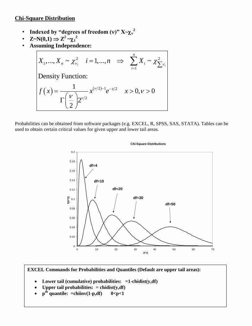
Chi-Square Distribution
• Indexed by “degrees of freedom ()” X~2
• Z~N(0,1) Z2 ~1
2
• Assuming Independence:
Probabilities can be obtained from software packages (e.g. EXCEL, R, SPSS, SAS, STATA). Tables can be
used to obtain certain critical values for given upper and lower tail areas.
2 2
1
1
2 1 2
2
,..., ~ 1,..., ~
Density Function:
10, 0
22
i i
n
n i
i
x
X X i n X
f x x e x
0
0.02
0.04
0.06
0.08
0.1
0.12
0.14
0.16
0.18
0.2
0 10 20 30 40 50 60 70
f(X
^2
)
X^2
Chi-Square Distributions
df=4
df=10
df=20
df=30
df=50
EXCEL Commands for Probabilities and Quantiles (Default are upper tail areas):
Lower tail (cumulative) probabilities: =1-chidist(y,df)
Upper tail probabilities: = chidist(y,df)
pth
quantile: =chiinv(1-p,df) 0<p<1

Critical Values for Chi-Square Distributions (Mean=, Variance=2)
df\F(x) 0.005 0.01 0.025 0.05 0.1 0.9 0.95 0.975 0.99 0.995
1 0.000 0.000 0.001 0.004 0.016 2.706 3.841 5.024 6.635 7.879
2 0.010 0.020 0.051 0.103 0.211 4.605 5.991 7.378 9.210 10.597
3 0.072 0.115 0.216 0.352 0.584 6.251 7.815 9.348 11.345 12.838
4 0.207 0.297 0.484 0.711 1.064 7.779 9.488 11.143 13.277 14.860
5 0.412 0.554 0.831 1.145 1.610 9.236 11.070 12.833 15.086 16.750
6 0.676 0.872 1.237 1.635 2.204 10.645 12.592 14.449 16.812 18.548
7 0.989 1.239 1.690 2.167 2.833 12.017 14.067 16.013 18.475 20.278
8 1.344 1.646 2.180 2.733 3.490 13.362 15.507 17.535 20.090 21.955
9 1.735 2.088 2.700 3.325 4.168 14.684 16.919 19.023 21.666 23.589
10 2.156 2.558 3.247 3.940 4.865 15.987 18.307 20.483 23.209 25.188
11 2.603 3.053 3.816 4.575 5.578 17.275 19.675 21.920 24.725 26.757
12 3.074 3.571 4.404 5.226 6.304 18.549 21.026 23.337 26.217 28.300
13 3.565 4.107 5.009 5.892 7.042 19.812 22.362 24.736 27.688 29.819
14 4.075 4.660 5.629 6.571 7.790 21.064 23.685 26.119 29.141 31.319
15 4.601 5.229 6.262 7.261 8.547 22.307 24.996 27.488 30.578 32.801
16 5.142 5.812 6.908 7.962 9.312 23.542 26.296 28.845 32.000 34.267
17 5.697 6.408 7.564 8.672 10.085 24.769 27.587 30.191 33.409 35.718
18 6.265 7.015 8.231 9.390 10.865 25.989 28.869 31.526 34.805 37.156
19 6.844 7.633 8.907 10.117 11.651 27.204 30.144 32.852 36.191 38.582
20 7.434 8.260 9.591 10.851 12.443 28.412 31.410 34.170 37.566 39.997
21 8.034 8.897 10.283 11.591 13.240 29.615 32.671 35.479 38.932 41.401
22 8.643 9.542 10.982 12.338 14.041 30.813 33.924 36.781 40.289 42.796
23 9.260 10.196 11.689 13.091 14.848 32.007 35.172 38.076 41.638 44.181
24 9.886 10.856 12.401 13.848 15.659 33.196 36.415 39.364 42.980 45.559
25 10.520 11.524 13.120 14.611 16.473 34.382 37.652 40.646 44.314 46.928
26 11.160 12.198 13.844 15.379 17.292 35.563 38.885 41.923 45.642 48.290
27 11.808 12.879 14.573 16.151 18.114 36.741 40.113 43.195 46.963 49.645
28 12.461 13.565 15.308 16.928 18.939 37.916 41.337 44.461 48.278 50.993
29 13.121 14.256 16.047 17.708 19.768 39.087 42.557 45.722 49.588 52.336
30 13.787 14.953 16.791 18.493 20.599 40.256 43.773 46.979 50.892 53.672
40 20.707 22.164 24.433 26.509 29.051 51.805 55.758 59.342 63.691 66.766
50 27.991 29.707 32.357 34.764 37.689 63.167 67.505 71.420 76.154 79.490
60 35.534 37.485 40.482 43.188 46.459 74.397 79.082 83.298 88.379 91.952
70 43.275 45.442 48.758 51.739 55.329 85.527 90.531 95.023 100.425 104.215
80 51.172 53.540 57.153 60.391 64.278 96.578 101.879 106.629 112.329 116.321
90 59.196 61.754 65.647 69.126 73.291 107.565 113.145 118.136 124.116 128.299
100 67.328 70.065 74.222 77.929 82.358 118.498 124.342 129.561 135.807 140.169

R Program to Obtain Probabilities, Percentiles, Density Functions, and Random Sampling
# Obtain P(Y<=5|X2(df=10))
# pchisq gives lower tail probabilities (cdf) for a chi-square distribution
pchisq(5,df=10)
# Obtain P(Y>=5|X2(df=10))
# lower=FALSE option gives upper tail probabilities
pchisq(5,df=10,lower=FALSE)
# Obtain the 95th percentile of a Chi-square Density with df=10
qchisq(0.95,df=10)
# Obtain a plot of a Chi-square Density with df=10
# dchisq gives the density function for a chi-square distribution at point(s) y
# type="l" in plot function joins the points on the density function with a line
# The polygon command fills in the area below y<5 in green
y <- seq(0,30,0.01)
fy <- dchisq(y,df=10)
# Output graph to a .png file in the following directory/file)
png("E:\\blue_drive\\Rmisc\\graphs\\chisq_dist1.png")
plot(y,fy,type="l",
main=expression(paste(chi^2,"(df=10)")))
polygon(c(y[y<=5],5),c(fy[y<=5],fy[y==0]),col="blue")
dev.off() # Close the .png file
# Obtain a random sample of 1000 items from Chi-square(df=10)
# rchisq gives a random sample of size given by the first argument
# Obtain sample mean, median, variance, standard deviation
set.seed(54321) # Set the seed for random number generator for reproducing data
y.samp <- rchisq(1000,df=10)
mean(y.samp)
median(y.samp)
var(y.samp)
sd(y.samp)
# Plot a histogram of the sample values (Default bin size)
hist(y.samp, main = expression(paste("Sampled values, ", chi^2, "(df=10)")))
# Allow for more bins
# Output graph to a .png file in the following directory/file)
png("E:\\blue_drive\\Rmisc\\graphs\\chisq_dist2.png")
hist(y.samp[y.samp<=30], breaks=29,
main = expression(paste("Sampled values, ", chi^2, "(df=10)")))
# Add chi-square density (scaled up by (n=1000 x binwidth=1), since a freq histogram)
# Makes use of y and fy defined above
lines(y,1000*1*fy)
dev.off() # Close the .png file

Numeric Output from R Program
Note that for the chi-square distribution, the mean is the degrees of freedom () and the variance is 2. The
sample mean and variance are close to 10 and 20. As the sample size gets larger, they will tend to get closer.
Also notice that the median is lower than the mean (right-skewed distribution).
Confirm that the 95th
-percentile is consistent with the table value.
Cell Result
A1 0.108822
A2 0.891178
A3 18.30704
>
> pchisq(5,df=10)
[1] 0.108822
>
> pchisq(5,df=10,lower=FALSE)
[1] 0.891178
>
> qchisq(0.95,df=10)
[1] 18.30704
> mean(y.samp)
[1] 9.834778
> median(y.samp)
[1] 9.060967
> var(y.samp)
[1] 21.78964
> sd(y.samp)
[1] 4.667937
EXCEL Output:
Cell A1: =1-CHIDIST(5,10)
Cell A2: =CHIDIST(5,10)
Cell A3: =CHIINV(0.05,10)

Graphics Output from R Program

Student’s t-Distribution
• Indexed by “degrees of freedom )” X~t
• Z~N(0,1), X~n2
• Assuming Independence of Z and X:
Probabilities can be obtained from software packages (e.g. EXCEL, R, SPSS, SAS, STATA). Tables can be
used to obtain certain critical values for given upper tail areas (distribution is symmetric around 0, as N(0,1) is.
~Z
T tX
0
0.05
0.1
0.15
0.2
0.25
0.3
0.35
0.4
0.45
-3 -2 -1 0 1 2 3
De
nsi
ty
t (z)
t(3), t(11), t(24), Z Distributions
f(t_3)
f(t_11)
f(t_24)
Z~N(0,1)
EXCEL Commands for Probabilities and Quantiles (Default are lower tail areas):
Lower tail (cumulative) probabilities: =t.dist(y,df,TRUE)
Upper tail probabilities: =1- t.dist(y,df,TRUE)
pth
quantile: =t.inv(p,df) 0<p<1

Critical Values for Student’s t-Distributions (Mean=0, Variance = )
df\F(t) 0.9 0.95 0.975 0.99 0.995
1 3.078 6.314 12.706 31.821 63.657
2 1.886 2.920 4.303 6.965 9.925
3 1.638 2.353 3.182 4.541 5.841
4 1.533 2.132 2.776 3.747 4.604
5 1.476 2.015 2.571 3.365 4.032
6 1.440 1.943 2.447 3.143 3.707
7 1.415 1.895 2.365 2.998 3.499
8 1.397 1.860 2.306 2.896 3.355
9 1.383 1.833 2.262 2.821 3.250
10 1.372 1.812 2.228 2.764 3.169
11 1.363 1.796 2.201 2.718 3.106
12 1.356 1.782 2.179 2.681 3.055
13 1.350 1.771 2.160 2.650 3.012
14 1.345 1.761 2.145 2.624 2.977
15 1.341 1.753 2.131 2.602 2.947
16 1.337 1.746 2.120 2.583 2.921
17 1.333 1.740 2.110 2.567 2.898
18 1.330 1.734 2.101 2.552 2.878
19 1.328 1.729 2.093 2.539 2.861
20 1.325 1.725 2.086 2.528 2.845
21 1.323 1.721 2.080 2.518 2.831
22 1.321 1.717 2.074 2.508 2.819
23 1.319 1.714 2.069 2.500 2.807
24 1.318 1.711 2.064 2.492 2.797
25 1.316 1.708 2.060 2.485 2.787
26 1.315 1.706 2.056 2.479 2.779
27 1.314 1.703 2.052 2.473 2.771
28 1.313 1.701 2.048 2.467 2.763
29 1.311 1.699 2.045 2.462 2.756
30 1.310 1.697 2.042 2.457 2.750
40 1.303 1.684 2.021 2.423 2.704
50 1.299 1.676 2.009 2.403 2.678
60 1.296 1.671 2.000 2.390 2.660
70 1.294 1.667 1.994 2.381 2.648
80 1.292 1.664 1.990 2.374 2.639
90 1.291 1.662 1.987 2.368 2.632
100 1.290 1.660 1.984 2.364 2.626
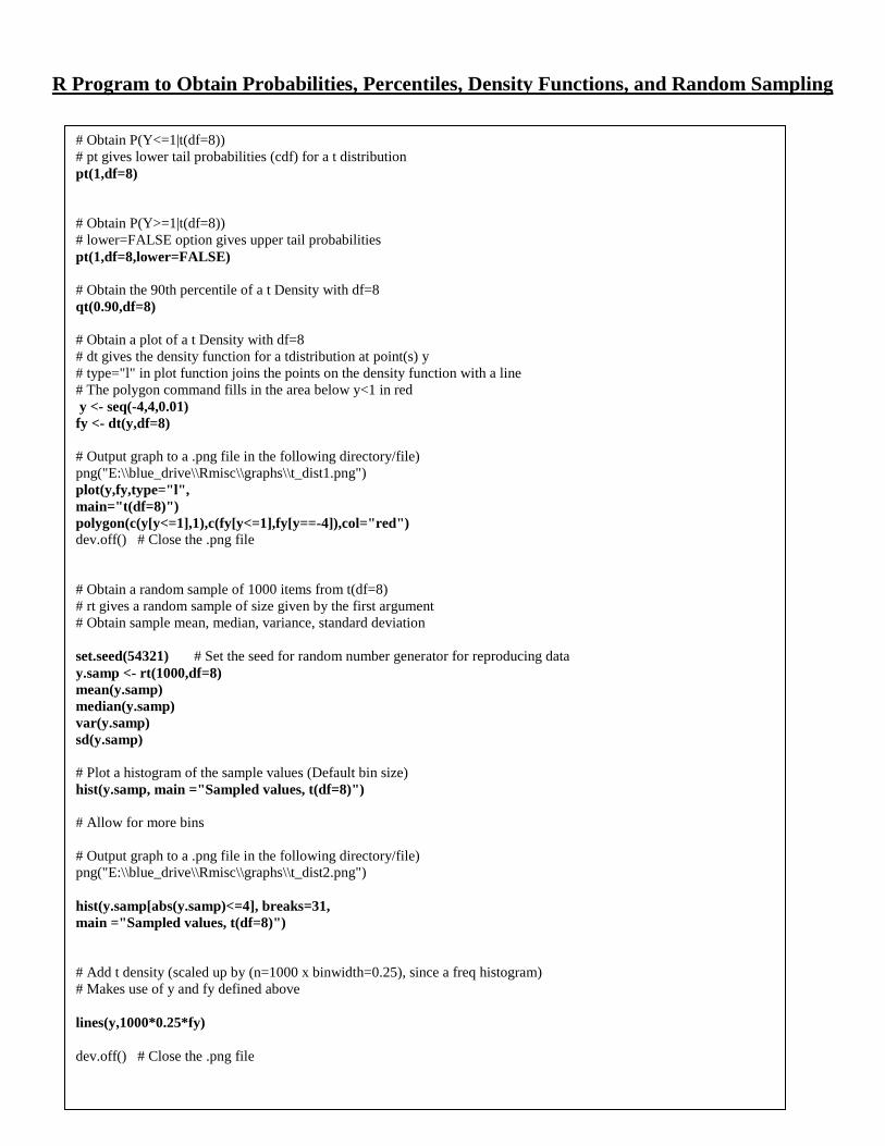
R Program to Obtain Probabilities, Percentiles, Density Functions, and Random Sampling
# Obtain P(Y<=1|t(df=8))
# pt gives lower tail probabilities (cdf) for a t distribution
pt(1,df=8)
# Obtain P(Y>=1|t(df=8))
# lower=FALSE option gives upper tail probabilities
pt(1,df=8,lower=FALSE)
# Obtain the 90th percentile of a t Density with df=8
qt(0.90,df=8)
# Obtain a plot of a t Density with df=8
# dt gives the density function for a tdistribution at point(s) y
# type="l" in plot function joins the points on the density function with a line
# The polygon command fills in the area below y<1 in red
y <- seq(-4,4,0.01)
fy <- dt(y,df=8)
# Output graph to a .png file in the following directory/file)
png("E:\\blue_drive\\Rmisc\\graphs\\t_dist1.png")
plot(y,fy,type="l",
main="t(df=8)")
polygon(c(y[y<=1],1),c(fy[y<=1],fy[y==-4]),col="red")
dev.off() # Close the .png file
# Obtain a random sample of 1000 items from t(df=8)
# rt gives a random sample of size given by the first argument
# Obtain sample mean, median, variance, standard deviation
set.seed(54321) # Set the seed for random number generator for reproducing data
y.samp <- rt(1000,df=8)
mean(y.samp)
median(y.samp)
var(y.samp)
sd(y.samp)
# Plot a histogram of the sample values (Default bin size)
hist(y.samp, main ="Sampled values, t(df=8)")
# Allow for more bins
# Output graph to a .png file in the following directory/file)
png("E:\\blue_drive\\Rmisc\\graphs\\t_dist2.png")
hist(y.samp[abs(y.samp)<=4], breaks=31,
main ="Sampled values, t(df=8)")
# Add t density (scaled up by (n=1000 x binwidth=0.25), since a freq histogram)
# Makes use of y and fy defined above
lines(y,1000*0.25*fy)
dev.off() # Close the .png file
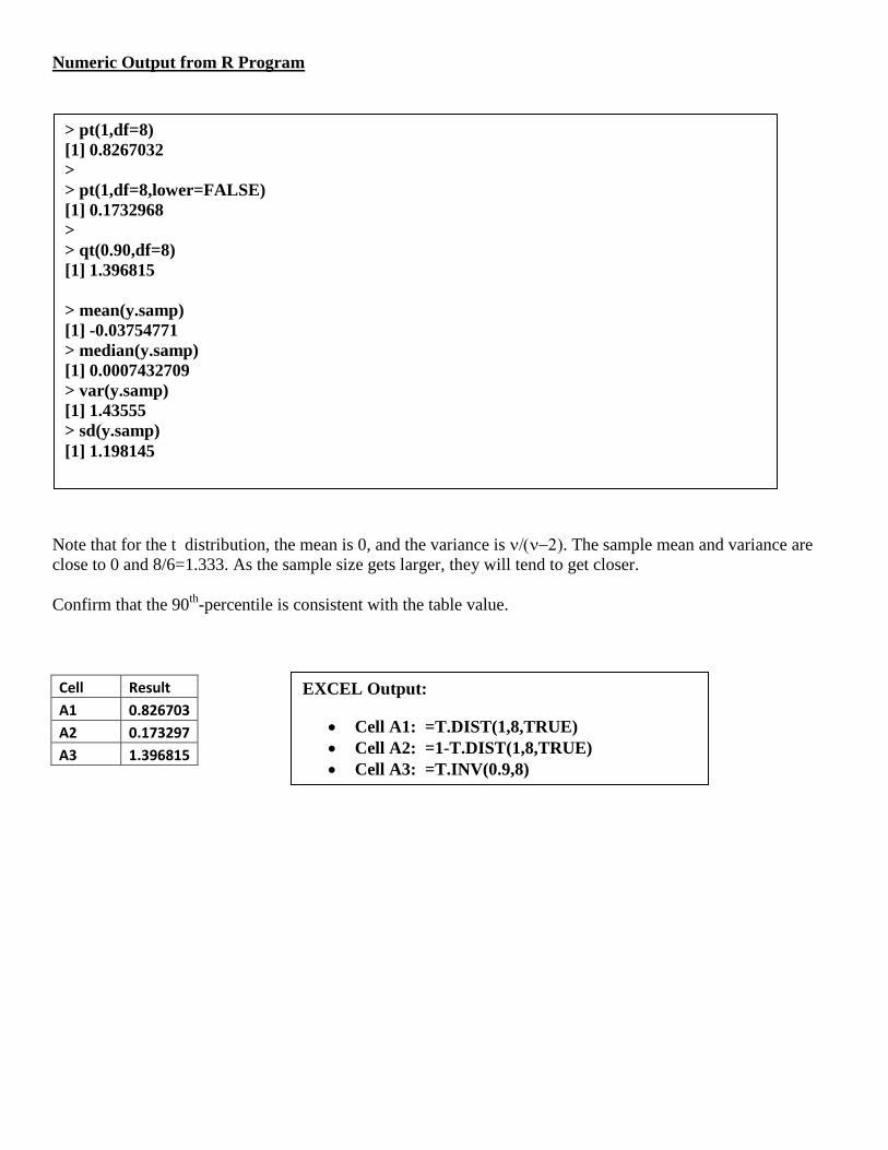
Numeric Output from R Program
Note that for the t distribution, the mean is 0, and the variance is . The sample mean and variance are
close to 0 and 8/6=1.333. As the sample size gets larger, they will tend to get closer.
Confirm that the 90th
-percentile is consistent with the table value.
Cell Result
A1 0.826703
A2 0.173297
A3 1.396815
> pt(1,df=8)
[1] 0.8267032
>
> pt(1,df=8,lower=FALSE)
[1] 0.1732968
>
> qt(0.90,df=8)
[1] 1.396815
> mean(y.samp)
[1] -0.03754771
> median(y.samp)
[1] 0.0007432709
> var(y.samp)
[1] 1.43555
> sd(y.samp)
[1] 1.198145
EXCEL Output:
Cell A1: =T.DIST(1,8,TRUE)
Cell A2: =1-T.DIST(1,8,TRUE)
Cell A3: =T.INV(0.9,8)

Graphics Output from R Program

F-Distribution
• Indexed by 2 “degrees of freedom (1,2)” W~F1,2
• X1 ~2, X2 ~
2
• Assuming Independence of X1 and X2:
Probabilities can be obtained from software packages (e.g. EXCEL, R, SPSS, SAS, STATA). Tables can be
used to obtain certain critical values for given upper tail areas. Lower tails are obtained by taking the reciprocal
of the upper tail with the degrees of freedom reversed.
1 11 2
2 2
~ ,X
W FX
-0.1
0
0.1
0.2
0.3
0.4
0.5
0.6
0.7
0.8
0.9
0 1 2 3 4 5 6 7 8 9 10
De
nsi
ty F
un
cti
on
of
F
F
F-Distributions
f(5,5)
f(5,10)
f(10,20)
EXCEL Commands for Probabilities and Quantiles (Default are upper tail areas):
Lower tail (cumulative) probabilities: =1-fdist(y,df1,df2)
Upper tail probabilities: = fdist(y,df1,df2)
pth
quantile: =finv(1-p,df1,df2) 0<p<1

Critical Values for F-distributions P(F ≤ Table Value) = 0.95
df2\df1 1 2 3 4 5 6 7 8 9 10
1 161.45 199.50 215.71 224.58 230.16 233.99 236.77 238.88 240.54 241.88
2 18.51 19.00 19.16 19.25 19.30 19.33 19.35 19.37 19.38 19.40
3 10.13 9.55 9.28 9.12 9.01 8.94 8.89 8.85 8.81 8.79
4 7.71 6.94 6.59 6.39 6.26 6.16 6.09 6.04 6.00 5.96
5 6.61 5.79 5.41 5.19 5.05 4.95 4.88 4.82 4.77 4.74
6 5.99 5.14 4.76 4.53 4.39 4.28 4.21 4.15 4.10 4.06
7 5.59 4.74 4.35 4.12 3.97 3.87 3.79 3.73 3.68 3.64
8 5.32 4.46 4.07 3.84 3.69 3.58 3.50 3.44 3.39 3.35
9 5.12 4.26 3.86 3.63 3.48 3.37 3.29 3.23 3.18 3.14
10 4.96 4.10 3.71 3.48 3.33 3.22 3.14 3.07 3.02 2.98
11 4.84 3.98 3.59 3.36 3.20 3.09 3.01 2.95 2.90 2.85
12 4.75 3.89 3.49 3.26 3.11 3.00 2.91 2.85 2.80 2.75
13 4.67 3.81 3.41 3.18 3.03 2.92 2.83 2.77 2.71 2.67
14 4.60 3.74 3.34 3.11 2.96 2.85 2.76 2.70 2.65 2.60
15 4.54 3.68 3.29 3.06 2.90 2.79 2.71 2.64 2.59 2.54
16 4.49 3.63 3.24 3.01 2.85 2.74 2.66 2.59 2.54 2.49
17 4.45 3.59 3.20 2.96 2.81 2.70 2.61 2.55 2.49 2.45
18 4.41 3.55 3.16 2.93 2.77 2.66 2.58 2.51 2.46 2.41
19 4.38 3.52 3.13 2.90 2.74 2.63 2.54 2.48 2.42 2.38
20 4.35 3.49 3.10 2.87 2.71 2.60 2.51 2.45 2.39 2.35
21 4.32 3.47 3.07 2.84 2.68 2.57 2.49 2.42 2.37 2.32
22 4.30 3.44 3.05 2.82 2.66 2.55 2.46 2.40 2.34 2.30
23 4.28 3.42 3.03 2.80 2.64 2.53 2.44 2.37 2.32 2.27
24 4.26 3.40 3.01 2.78 2.62 2.51 2.42 2.36 2.30 2.25
25 4.24 3.39 2.99 2.76 2.60 2.49 2.40 2.34 2.28 2.24
26 4.23 3.37 2.98 2.74 2.59 2.47 2.39 2.32 2.27 2.22
27 4.21 3.35 2.96 2.73 2.57 2.46 2.37 2.31 2.25 2.20
28 4.20 3.34 2.95 2.71 2.56 2.45 2.36 2.29 2.24 2.19
29 4.18 3.33 2.93 2.70 2.55 2.43 2.35 2.28 2.22 2.18
30 4.17 3.32 2.92 2.69 2.53 2.42 2.33 2.27 2.21 2.16
40 4.08 3.23 2.84 2.61 2.45 2.34 2.25 2.18 2.12 2.08
50 4.03 3.18 2.79 2.56 2.40 2.29 2.20 2.13 2.07 2.03
60 4.00 3.15 2.76 2.53 2.37 2.25 2.17 2.10 2.04 1.99
70 3.98 3.13 2.74 2.50 2.35 2.23 2.14 2.07 2.02 1.97
80 3.96 3.11 2.72 2.49 2.33 2.21 2.13 2.06 2.00 1.95
90 3.95 3.10 2.71 2.47 2.32 2.20 2.11 2.04 1.99 1.94
100 3.94 3.09 2.70 2.46 2.31 2.19 2.10 2.03 1.97 1.93

R Program to Obtain Probabilities, Percentiles, Density Functions, and Random Sampling
# Obtain P(Y<=2.5|F(df1=10,df2=8))
# pf gives lower tail probabilities (cdf) for a F distribution
pf(2.5,df1=10,df2=8)
# Obtain P(Y>=2.5|F(df1=10,df2=8)))
# lower=FALSE option gives upper tail probabilities
pf(2.5,df1=10,df2=8,lower=FALSE)
# Obtain the 5th and 95th percentiles of a F Density with df1=10,df2=8
qf(0.05,df1=10,df2=8)
qf(0.95,df1=10,df2=8)
# Obtain a plot of a F Density with df1=10, df2=8
# df gives the density function for a F distribution at point(s) y
# type="l" in plot function joins the points on the density function with a line
# The polygon command fills in the area below y<2.5 in purple
y <- seq(0,10,0.01)
fy <- df(y,df1=10,df2=8)
# Output graph to a .png file in the following directory/file)
png("E:\\blue_drive\\Rmisc\\graphs\\f_dist1.png")
plot(y,fy,type="l",
main="F(df1=10,df2=8)")
polygon(c(y[y<=2.5],2.5),c(fy[y<=2.5],fy[y==0]),col="purple")
dev.off() # Close the .png file
# Obtain a random sample of 1000 items from F(df1=10,df2=8)
# rf gives a random sample of size given by the first argument
# Obtain sample mean, median, variance, standard deviation
set.seed(54321) # Set the seed for random number generator for reproducing data
y.samp <- rf(1000,df1=10,df2=8)
mean(y.samp)
median(y.samp)
var(y.samp)
sd(y.samp)
# Plot a histogram of the sample values (Default bin size)
hist(y.samp, main ="Sampled values, F(df1=10,df2=8)")
# Allow for more bins
# Output graph to a .png file in the following directory/file)
png("E:\\blue_drive\\Rmisc\\graphs\\f_dist2.png")
hist(y.samp[y.samp<=10], breaks=19, ylim=c(0,400),
main ="Sampled values, F(df1=10,df2=8)")
# Add chi-square density (scaled up by (n=1000 x binwidth=0.5), since a freq histogram)
# Makes use of y and fy defined above
lines(y,1000*0.5*fy)
dev.off() # Close the .png file

Numeric Output from R Program
Note that for the F distribution, the mean and variance formulas are given below.
2
2 1 222 22
2 1 2 2
2 2Mean: 2 Variance: 4
2 2 4
For this case, the mean is 8/6 = 1.333 and the variance is 2048/1440 = 1.422. Again the sample mean and
variance would tend to be closer to the theoretical values as the sample size increases.
Confirm the 5th
and 95th
percentiles based on the F-table. Again note that the lower percentile can be obtained
by taking the reciprocal of the upper percentile with the degrees of freedom reversed.
Cell Result
A1 0.896406
A2 0.103594
A3 0.325557
A4 3.347163
> pf(2.5,df1=10,df2=8)
[1] 0.8964058
>
> pf(2.5,df1=10,df2=8,lower=FALSE)
[1] 0.1035942
>
> qf(0.05,df1=10,df2=8)
[1] 0.325557
> qf(0.95,df1=10,df2=8)
[1] 3.347163
> mean(y.samp)
[1] 1.369505
> median(y.samp)
[1] 1.059021
> var(y.samp)
[1] 1.50341
> sd(y.samp)
[1] 1.226136
EXCEL Output:
Cell A1: =1-FDIST(2.5,10,8)
Cell A2: =FDIST(2.5,10,8)
Cell A3: =FINV(0.95,10,8)
Cell A4: =FINV(0.05,10,8)

Graphics Output from R Program

Statistical Estimation: Properties
Note: If an estimator is unbiased (easy to show) and its variance goes to zero as its sample size gets
infinitely large (easy to show), it is consistent. It is tougher to show that it is Minimum Variance, but
general results have been obtained in many standard cases.
Statistical Estimation: Methods
^
1
^
^
Parameter: Estimator: function of ,...,
1) Unbiased:
2) Consistent: lim 0 for any > 0
3) Sufficient if conditional joint probability of sam
Properties of Estimators:
n
n
Y Y
E
P
^
* *^ ^ ^2 2
ple, given does not depend on
4) Minimum Variance: for all
1
1
1
~ ; Probability function for that depends on parameter
Random Sample (independent) ,..., with joint probability function:
,..., ;
When viewe
Maximum Likelihood (ML) Estimators:
n
n
n
i
Y f Y Y
Y Y
g Y Y f Y
1
d as function of , given the observed data (sample):
Likelihood function: ; Goal: maximize with respect to .
Under general conditions, ML estimators are consistent and suffic
n
i
L f Y L
2
1
ient
where is a known function of the parameter and are random variables, usually with =0
Sum of Squares: Goal: minimiz
Least Squares (LS) Estimators
i i i
i i i
n
i i
i
Y f
f E
Q Y f
e with respect to .
In many settings, LSestimators are unbiased and consistent.
Q

One-Sample Confidence Interval for
• Simple Random Sample (SRS) from a population with mean is obtained.
• Sample mean, sample standard deviation are obtained
• Degrees of freedom are df= n-1, and confidence level (1-) are selected
• Level (1-) confidence interval of form:
Procedure is theoretically derived based on normally distributed data, but has been found to work well
regardless for moderate to large n
Example: Mercury Levels Albacore Fish in the Eastern Mediterranean
Sample: n = 34 albacore fish caught in the Eastern Mediterranean Sea. Response is Mercury level (mg/kg).
Goal: Treating this as a random sample of all albacore in the area, obtain 95% Confidence Interval for the
population mean mercury level.
Fish 1 2 3 4 5 6 7 8 9 10 11 12
Mercury 1.007 1.447 0.763 2.01 1.346 1.243 1.586 0.821 1.735 1.396 1.109 0.993
Fish 13 14 15 16 17 18 19 20 21 22 23 24
Mercury 2.007 1.373 2.242 1.647 1.35 0.948 1.501 1.907 1.952 0.996 1.433 0.866
Fish 25 26 27 28 29 30 31 32 33 34 Mean StdDev
Mercury 1.049 1.665 2.139 0.534 1.027 1.678 1.214 0.905 1.525 0.763 1.358147 0.440703
If all possible random samples of size 34 had been obtained, and this calculation had been made for each
sample, then 95% of all sample Confidence Intervals would contain the true unknown population mean level .
Thus we can be 95% confident that is between 1.2043 and 1.5119. Note that 90% and 99% Confidence
Intervals based on this same sample are as follow (confirm them, and why the lengths differ):
90% Confidence Interval for (1.2302 , 1.4861) 90% Confidence Interval for (1.1516 , 1.5647)
2
21 11 / 2; 11
n n
i i
i i
Y Y Y
Y ss
Y t n s Yn n
s Yn
1 0.95 0.05 34
1 / 2; 1 1 0.05 / 2;34 1 0.975;33 2.0345
0.44071.3581 0.4407 0.0756
34
1 / 2; 1 1.3581 2.0345(0.0756)
1.3581 0.1538 1.2043 ,1.5119
n
t n t t
sY s s Y
n
Y t n s Y

1-Sample t-test (2-tailed alternative)
• 2-sided Test: H0: = 0 Ha: 0
• Decision Rule :
– Conclude > 0 if Test Statistic (t*) > t(1-/2;n-1)
– Conclude < 0 if Test Statistic (t*) <- t(1-/2;n-1)
– Do not conclude Conclude 0 otherwise
• P-value: 2P(t(n-1) |t*|)
• Test Statistic:
1-tailed alternative tests
0 0 0
0
0 0 0
0
Upper Tailed : :
Decision Rule: Reject if * 1 ; 1
-value: 1 *
Lower Tailed : :
Decision Rule: Reject if * 1 ; 1
-value: 1 *
A
A
H H
H t t n
P P t n t
H H
H t t n
P P t n t
Note: Tests for are generally used when trying to show whether a mean differs from, is above or below some
pre-specified value; or when the data are paired differences (such as before/after treatment measures).
Example: The European Union has permissible limit of 1 mg/kg of Mercury in fish. Is > 1?
0 0 0
00
: 1 : 1
1.3581 1: * 4.7836 0.95;33 1.6924 Reject , Conclude 1
0.0756
-value: (33) 4.7836 .00002
AH H
YTS t t H
s Y
P P t
0*
Y st s Y
ns Y

Comparing 2 Means - Independent Samples
• Observed individuals/items from the 2 groups are samples from distinct populations
(identified by () and (
))
• Measurements across groups are independent
• Summary statistics obtained from the 2 groups
Sampling Distribution of Y Z
• Underlying distributions normal sampling distribution is normal, and resulting t-distribution
with estimated std. dev.
• Mean, variance, standard error (Std. Dev. of estimator)
11
1 1
2 2
2
111
1 1
1
Group 1: Mean: Std. Dev.: Sample Size:
Group 2: Mean: Std. Dev.: Sample Size:
similar calculations for 1
In many settings, we replace ,...,
nn
ii ii
Y s n
Z s n
Y YYY s Z
n n
Y Y
1 1 2 211 1 1 21 2
1 2
with ,..., and ,..., with ,...,n n n nY Y Z Z Y Y
Y Y Z Y
1 2
2 2 2 22 2 1 2 1 2
1 2 1 2
1 22 2
1 2 1 2
2 2
1 1 2 22
1 2 1 2
~ with df = 2
1 11 1where:
2
Y Z
Y Z Y Z
E Y Z
Y Zn n n n
Y Zt n n
s Y Z
n s n ss Y Z s s
n n n n

Inference for - Normal Populations – Equal variances
• Interpretation (at the significance level):
– If interval contains 0, do not reject H0:
– If interval is strictly positive, conclude that
– If interval is strictly negative, conclude that
Example – Children’s Participation in Meal Preparation and Caloric Intake
Experiment had 2 conditions: Child participated in Cooking Meal, and Parent only cooking meal. Response
measured: Total Energy Intake (kcals). Total of 47 participants: 25 in Child cooks (Y), 22 in Parent cooks (Z).
1 1 2 2
2 2 2 2
1 1 2 22
1 2
Child Cooks: 431.4 105.7 25 Parent Cooks: 346.8 99.5 22
431.4 346.8 84.6 1 .05 / 2;25 22 2 .975;45 2.0141
1 1 25 1 105.7 22 1 99.5 47604510578.78 10
2 25 22 2 45
Y s n Z s n
Y Z t t
n s n ss s
n n
1 2
1 2
0 1 2 1 2
2.8532
1 1 1 1102.8532 102.8532 0.2923 30.0667
25 22
95% CI for : .975;45 84.6 2.0141(30.0667) 84.6 60.6 24.0 ,145.2
Testing: : 0 vs : 0
84.6: *
30
A
s Y Z sn n
Y Z t s Y Z
H H
Y ZTS t
s Y Z
2.8137 .975;45 2.0141 2 (45) 2.8137 2(.0036) .0072
.0667t P P t
1 2
1 100% Confidence Interval:
1 / 2; 2Y Z t n n s Y Z
0 1 2 1 2
1 2
: 0 : 0
Test Stat : *
Reject Reg : * 1 / 2; 2
AH H
Y Zt
s Y Z
t t n n

Sampling Distribution of s2
(Normal Data)
• Population variance (
) is a fixed (unknown) parameter based on the population of
measurements
• Sample variance (s2) varies from sample to sample (just as sample mean does)
• When Y~N(), the distribution of (a multiple of) s
2 is Chi-Square with n-1 degrees of
freedom. Unlike inference on means, the normality assumption is very important.
• (n-1)s2/
with df=n-1
(1-a)100% Confidence Interval for (or )
• Step 1: Obtain a random sample of n items from the population, compute s2
• Step 2: Obtain 2L and 2
U from table of critical values for chi-square distribution with n-
1 df
• Step 3: Compute the confidence interval for 2 based on the formula below and take
square roots of bounds for 2 to obtain confidence interval for
Example: Mercury Levels in Albacore Fish from Eastern Mediterranean (Continued)
2 2 2 2 2
2 2 2
2 22
2 2
1 0.95 0.05 / 2 0.025 1 / 2 0.975
34 1 / 2; 1 .975;33 50.73 .025;33 19.05
0.4407 0.4407 0.1942 1 33(0.1942) 6.4092
( 1) ( 1) 6.4092(1 )100% CI for : ,
50.7
U L
U L
n n
s s n s
n s n s
6.4092, 0.1263 , 0.3364
3 19.05
(1 )100% CI for : 0.1263 , 0.3364 0.3364 , 0.5800
2 22
2 2
2 2 2 2
( 1) ( 1)(1 )100% CI for : ,
where: 1 / 2; 1 / 2; 1
U L
U L
n s n s
n n

Statistical Test for 2
• Null and alternative hypotheses
– 1-sided (upper tail): H0: 0
2 Ha:
2 > 0
2
– 1-sided (lower tail): H0: 2 0
2 Ha:
2 < 0
2
– 2-sided: H0: 2 = 0
2 Ha:
2 0
2
• Test Statistic
• Decision Rule based on chi-square distribution w/ df=n-1:
– 1-sided (upper tail): Reject H0 if obs2 > U
2 = 2
(1-;n-1)
– 1-sided (lower tail): Reject H0 if obs2 < L
2 = 2
(;n-1)
– 2-sided: Reject H0 if obs2 < L
2 = 2
(/2;n-1)(Conclude 2 < 0
2)
or if obs2 > U
2 = 2
(1-/2;n-1) (Conclude 2
> 02 )
There are not too many practical cases where there is a null value to test, except in cases where firms may need
to demonstrate that variation in purity of a chemical or compound is below some nominal level, or that variation
in measurements of manufactured parts is below some nominal level.
Note that most decisions can be obtained based on the confidence interval for the population variance (or
standard deviation).
22
2
0
( 1)obs
n s

Inferences Regarding 2 Population Variances
• Goal: Compare variances between 2 populations
• Parameter: (Ratio is 1 when variances are equal)
• Estimator: (Ratio of sample variances)
• Distribution of (multiple) of estimator (Normal Data):
Test Comparing Two Population Variances
(1-)100% Confidence Interval for 12/2
2
• Obtain ratio of sample variances s12/s2
2 = (s1/s2)
2
• Choose , and obtain:
– FL = F(/2, n1-1, n2-1) = 1/ F(1-/2, n2-1, n1-1)
– FU = F(1-/2, n1-1, n2-1)
• Compute Confidence Interval:
Conclude population variances unequal if interval does not contain 1
2
1
2
2
2
1
2
2
s
s
2 2 2 2
1 1 1 21 1 2 22 2 2 2
2 2 1 2
~ with df 1 and df 1s s s
F n ns
2 2 2 2
0 1 2 1 2
2
11 22
2
2 2 2 2
0 1 2 1 2
2
1
2
2
1-Sided Test: : :
Test Statistic: Rejection Region: 1 ; 1, 1 value: ( )
2-Sided Test: : :
Test Statistic:
Rejection Region:
a
obs obs obs
a
obs
ob
H H
sF F F n n P P F F
s
H H
sF
s
F
2 2
1 2 1 2
2 2
1 2 2 1 1 2
1 / 2; 1, 1 ( )
or / 2; 1, 1 =1/ 1 / 2; 1, 1 ( )
value: 2min( ( ), ( ))
s
obs
obs obs
F n n
F F n n F n n
P P F F P F F
2 2
1 1
2 2
2 2
,L U
s sF F
s s

Example – Children’s Participation in Meal Preparation and Caloric Intake (Continued)
2 2 2 2
0 1 2 1 2
2 2
1
2 2
2
2 2
1 2 1 2
2-Sided Test: : :
105.7Test Statistic: 1.13
99.5
Rejection Region: 1 / 2; 1, 1 1 .025;25 1,22 1 .975;24,21 2.3675 ( )
or .025;24,21 =1/ .975;21,
a
obs
obs
obs
H H
sF
s
F F n n F F
F F F
2 2
1 2
2
1
2
2
2 2
1 1
2 2
2 2
24 0.4327 ( )
value: 2min( ( ), ( )) 2min .3912,.6088 0.7824
95% Confidence Interval for
.025;24,21 1/ .975;21,24 0.4327
.975;24,21 2.3675
, 1.13(0.4
obs obs
L
U
L U
P P F F P F F
F F F
F F
s sF F
s s
327) ,1.13(2.3675) 0.49 , 2.68
What do you conclude?
Data Sources:
New York City Street Café’s:
https://nycopendata.socrata.com/Business/Sidewalk-Cafes/6k68-kc8u
Women’s Professional Soccer:
http://www.nwslsoccer.com/
Irish Premier League Soccer:
www.soccerpunter.com/
Mercury Levels in Albacore:
S. Mol, O. Ozden, S. Karakulak (2012). "Levels of Selected Metals in Albacore (Thunnus alalunga, Bonaterre, 1788) from the Eastern
Mediterranean, Journal of Aquatic Food Product Technology, Vol. 21, #2, pp. 111-117.
Children/Parent Cooking Effects on Food Intake:
K. van der Horst, A. Ferrage, A. Rytz (2014). “Involving Children in Meal Preparation: Effects on Food Intake,” Appetite, Vol. 79, pp.
18-24.

Chapter 1 – Linear Regression with 1 Predictor
Statistical Model
Y X i ni i i 0 1 1, ,
where:
Yi is the (random) response for the ith
case
0 1, are parameters
X i is a known constant, the value of the predictor variable for the ith
case
i is a random error term, such that: E i j i ji i i j{ } { } { , } , 0 02 2
The last point states that the random errors are independent (uncorrelated), with mean 0, and variance 2 . This
also implies that:
E Y X Y Y Yi i i i j{ } { } { , } 0 1
2 2 0
Thus, 0 represents the mean response when X 0 (assuming that is reasonable level of X ), and is referred to
as the Y-intercept. Also, 1 represent the change in the mean response as X increases by 1 unit, and is called
the slope.
Least Squares Estimation of Model Parameters
In practice, the parameters 0 and 1 are unknown and must be estimated. One widely used criterion is to
minimize the error sum of squares:
Y X Y X
Q Y X
i i i i i i
ii
n
i
n
i i
0 1 0 1
2
1 10 1
2
( )
( ( ))
This is done by calculus, by taking the partial derivatives of Q with respect to 0 and 1 and setting each
equation to 0. The values of 0 and 1 that set these equations to 0 are the least squares estimates and are
labelled b0 and b1 .
First, take the partial derivatives of Q with respect to 0 and 1 :
QY X
QY X X
i
n
i i
i
n
i i i
0 10 1
0 10 1
2 1 1
2 2
( ( ))( ) ( )
( ( ))( ) ( )

Next, set these 2 equations to 0, replacing 0 and 1 with b0 and b1 since these are the values that minimize
the error sum of squares:
2 0 1
2 0 2
0 11
0 11 1
0 11
01
11
2
1
( ) ( )
( ) ( )
Y b b X Y nb b X a
Y b b X X X Y b X b X a
i ii
n
ii
n
ii
n
i i ii
n
i i ii
n
i
n
ii
n
These two equations are referred to as the normal equations (although, note that we have said nothing YET,
about normally distributed data).
Solving these two equations yields:
b
X X Y Y
X X
X X
X X
Y k Y
b Y b Xn
Xk Y l Y
i ii
n
ii
n
i
ii
ni
n
i i ii
n
ii
n
i i ii
n
1
1
2
1
2
1
1 1
0 11 1
1
( )( )
( )
( )
( )
where k i and li are constants, and Yi is a random variable with mean and variance given above:
2 2
1 1
( )1 1
( ) ( )
i ii i in n
i i
i i
X X X X Xk l Xk
n nX X X X
The fitted regression line, also known as the prediction equation is:
Y b b X^
0 1
The fitted values for the individual observations are obtained by plugging in the corresponding level of the
predictor variable ( X i ) into the fitted equation. The residuals are the vertical distances between the observed
values (Yi ) and their fitted values (Y i
^
), and are denoted as ei .
Y b b X e Y Yi i i i i
^ ^
0 1

Properties of the fitted regression line
eii
n
1
0 The residuals sum to 0
X ei ii
n
1
0 The sum of the weighted (by X ) residuals is 0
Y ei ii
n ^
1
0 The sum of the weighted (by Y^
) residuals is 0
The regression line goes through the point ( X Y, )
These can be derived via their definitions and the normal equations:
^ ^
0 1 0 1
1 1 1 1 1 1
^ ^2
0 1 0 1
1 1 1 1 1 1 1
0 (1 )
0 (2 )
n n n n n n
i ii i i i i
i i i i i i
n n n n n n n
i ii i i i i i i i i i i
i i i i i i i
Y b b X nb b X Y Y Y e a
X Y X b b X b X b X X Y X Y Y X e a
Estimation of the Error Variance
Note that for a random variable, its variance is the expected value of the squared deviation from the mean. That
is, for a random variable W , with mean W its variance is:
2 2{ } {( ) }W E W W
For the simple linear regression model, the errors have mean 0, and variance 2 . This means that for the actual
observed values Yi , their mean and variance are as follows:
22 2
0 1 0 1{ } { }i i i i iE Y X Y E Y X
First, we replace the unknown mean 0 1 X i with its fitted value Y b b Xi i
^
0 1 , then we take the “average”
squared distance from the observed values to their fitted values. We divide the sum of squared errors by n-2 to
obtain an unbiased estimate of 2 (recall how you computed a sample variance when sampling from a single
population).
s
Y Y
n
e
n
i i
i
n
ii
n
2
2
1
2
1
2 2
( )^
Common notation is to label the numerator as the error sum of squares (SSE).
SSE Y Y ei i
i
n
ii
n
( )^
2
1
2
1

Also, the estimated variance is referred to as the error (or residual) mean square (MSE).
MSE sSSE
n
2
2
To obtain an estimate of the standard deviation (which is in the units of the data), we take the square root of the
error mean square. s MSE .
A shortcut formula for the error sum of squares, which can cause problems due to round-off errors is:
SSE Y Y b X X Y Yii
n
i ii
n
( ) ( )( )2
11
1
Some notation makes life easier when writing out elements of the regression model:
2
2
12 2 2
1 1 1
1 1
1 1 1
2
2
12 2 2
1 1 1
( )
( )( )
( )
n
in n ni
XX i i i
i i i
n n
i in n ni i
XY i i i i i i
i i i
n
in n ni
YY i i i
i i i
X
SS X X X X n Xn
X Y
SS X X Y Y X Y X Y nXYn
Y
SS Y Y Y Y n Yn
Note that we will be able to obtain most all of the simple linear regression analysis from these quantities, the
sample means, and the sample size.
2
2
1 0 1 1
( )
2
XY XYYY YY XY
XX XX
SS SS SSEb b Y b X SSE SS SS b SS s MSE
SS SS n
Normal Error Regression Model (Assumes STA 4322)
If we add further that the random errors follow a normal distribution, then the response variable also has a
normal distribution, with mean and variance given above. The notation, we will use for the errors, and the data
is:
i i iN Y N X~ ( , ) ~ ( , )0 2
0 1
2
The density function for the ith
observation is:
fY X
i
i i
1
2
1
2
0 1
2
exp

The likelihood function, is the product of the individual density functions (due to the independence assumption
on the random errors).
L Y X
Y X
i
n
i i
n i ii
n
( , , )( )
exp ( )
( )exp ( )
/
/
0 1
2
2 1 21
2 0 1
2
2 2 2 0 1
2
1
1
2
1
2
1
2
1
2
The values of 0 1
2, , that maximize the likelihood function are referred to as maximum likelihood
estimators. The MLE’s are denoted as: 0 1 2, ,^ ^ ^
. Note that the natural logarithm of the likelihood is
maximized by the same values of 0 1
2, , that maximize the likelihood function, and it’s easier to work with
the log likelihood function.
log log( ) log( ) ( )e i ii
n
Ln n
Y X
2
22
1
2
2
2 0 1
2
1
Taking partial derivatives with respect to 0 1
2, , yields:
0 1 0 12 21 10 1
2
0 12 2 2 21
log 1 log 12 ( )( 1) (4) 2 ( )( ) (5)
2 2
log 1( ) (6)
2 2( )
n n
i i i i i
i i
n
i i
i
L LY X Y X X
L nY X
Setting these three equations to 0, and placing “hats” on parameters denoting the maximum likelihood
estimators, we get the following three equations:
^ ^ ^ ^
2
0 1 0 1
1 1 1 1 1
^ ^2
0 14 2^ ^1
(4 ) (5 )
1( ) (6 )
n n n n n
i i i i i i
i i i i i
n
i i
i
Y n X a X Y X X a
nY X a
From equations 4a and 5a, we see that the maximum likelihood estimators are the same as the least squares
estimators (these are the normal equations). However, from equation 6a, we obtain the maximum likelihood
estimator for the error variance as:
^
^ ^ ^
( ) ( )2 0 1
2
1
2
1
Y X
n
Y Y
n
i ii
n
i i
i
n
This estimator is biased downward. We will use the unbiased estimator s MSE2 throughout this course to
estimate the error variance.

Example – U.S. State Non-Fuel Mineral Production vs Land Area (2011).
Non-Fuel mineral production ($10M) and land area (1000m2) for the 50 United States in 2011.
Source: http://minerals.er.usgs.gov/minerals/pubs/commodity/statistical_summary/index.html#myb
(retrieved 6/23/2014).
The following EXCEL spreadsheet gives the data in a form that is easier to read. The original data are in an
EXCEL file in Columns A-C and Rows 1-51 (variable names in row 1, numeric data in rows 2-51). Note that
Column A contains the state postal abbreviation, B contains Area, and C contains mineral production.
state Area Mineral state Area Mineral state Area Mineral state Area Mineral state Area Mineral
AL 50.74 96.0 HI 6.42 10.1 MA 7.84 22.5 NM 121.36 125.0 SD 75.89 31.2
AK 567.40 381.0 ID 82.75 132.0 MI 58.11 241.0 NY 47.21 134.0 TN 41.22 87.8
AZ 113.64 839.0 IL 55.58 107.0 MN 79.61 449.0 NC 48.71 84.3 TX 261.80 303.0
AR 52.07 78.9 IN 35.87 76.2 MS 46.91 19.5 ND 68.98 12.5 UT 82.14 430.0
CA 155.96 321.0 IA 55.87 65.3 MO 68.89 220.0 OH 40.95 96.2 VT 9.25 11.8
CO 103.72 193.0 KS 81.82 112.0 MT 145.55 144.0 OK 68.67 60.8 VA 39.59 119.0
CT 4.85 15.6 KY 39.73 79.1 NE 76.87 23.8 OR 96.00 30.5 WA 66.54 74.2
DE 1.95 1.1 LA 43.56 46.5 NV 109.83 1000.0 PA 44.82 160.0 WV 24.23 32.4
FL 53.93 343.0 ME 30.86 11.8 NH 8.97 10.0 RI 1.05 4.2 WI 54.31 68.3
GA 57.91 145.0 MD 9.77 29.3 NJ 7.42 27.5 SC 30.11 48.3 WY 97.11 214.0
Which variable is more likely to “cause” the other variable?
AREA → MINERAL or MINERAL → AREA
While we will use R for statistical analyses this semester that would be way too time consuming (if even
possible) in EXCEL, EXCEL does have some nice built-in functions to make calculations on ranges of cells.
=COUNT(range) - Computes the number of values in the range
=SUM(range) - Computes the sum for the values in the range
=AVERAGE(range) - Computes the sample mean for the values in the range
=VAR(range) - Computes the sample mean for the values in the range
=STDEV(range) - Computes the sample mean for the values in the range
=SUMSQ(range) - Computes the sum of squares for the values in the range
=DEVSQ(range) - Computes the sum of squared deviations from the mean
=SUMPRODUCT(range1,range2) - Computes the sum of products of each pair of elements of 2
ranges of equal length
=COVAR(range1,range2) - Computes the covariance of two ranges of equal length, using n as the
denominator, not n-1. In later versions, =COVARIANCE.S(range1,range2) is available, using n-1.
Making use of these, we can “brute-force” obtain the estimated regression equation and estimated error
variance. First, obtain the means and sums of squares and cross-products needed to obtain the regression
equation.

1 1
2
1
2 22
1 1 1
1
: COUNT B2:B51 : SUM B2:B51 : SUM C2:C51
: AVERAGE B2:B51 : AVERAGE C2:C51 : SUMSQ B2:B51
: SUMSQ C2:C51 : DEVSQ B2:B51 : DEVSQ C2:C51
: SUMPRODUCT B2:B51,C2
n n
i i
i i
n
i
i
n n n
i i i
i i i
n
i i
i
n X Y
X Y X
Y X X Y Y
X Y
1
1:C51 : COVAR B2:B51,C2:C51
n
i i
i
X X Y Yn
n 50.00 sum(Y^2) 2975248.32
X-bar 70.69 sum(XY) 856554.66
Y-bar 147.35 SS_XX 357703.85
sum(X) 3534.29 SS_YY 1889585.31
sum(Y) 7367.71 COV(X,Y) 6715.24
sum(X^2) 607528.11 SS_XY 335762.03
2
1
2
2
12
1
2
2 2
1
( ) 357703.85
3534.29607528.1 _________________________________________
50
607528.1 50(70.69) _________________________________________
( )
n
XX i
i
n
ini
i
i
n
i
i
XY i
SS X X
X
Xn
X n X
SS X X
1 1
1 1
1
1
1( ) ( )( ) 50 6715.24 335762
(3534.29)(7367.71)856554.66 ______________________________________
50
856554.66 50(7
n n
i i i
i i
n n
i ini i
i i
i
n
i i
i
Y Y n X X Y Yn
X Y
X Yn
X Y nXY
2
1
2
212
1
2
2
1
0.69)(147.35) _________________________________________
( ) 1889585.31
(7367.71)2975248.32 _________________________________________
50
2975248.32 50
n
YY i
i
n
ini
i
i
n
i
i
SS Y Y
Y
Yn
Y n Y
2(147.35) _________________________________________
Next compute the estimated regression coefficients, fitted equation, and estimated error variance and standard
deviation.
Note that when using formulas
with “multiple steps” you will find
there are “small” rounding errors.

1 0 1
^ ^
1
3357620.9387 147.35 0.9387(70.69) 80.9933
357703.85
80.99 0.94 or using symbols better related to data: 80.99 0.94
For State 1 (Alabama): Area = 50.74 and Mineral =
XY
XX
SSb b Y b X
SS
Y X M A
X
1
^ ^
1 10 1 1 1 1
2^
2
1 1
2 2
2
96.0
80.99 0.94(50.74) 80.99 47.70 128.69 96.0 128.69 32.69
( ) (335762)1889585.31 1889585.31 315166.08 1574419.23
357703.85
n n
ii i
i i
XYYY
XX
Y
Y b b X e Y Y
SSE Y Y e
SSSS
SS
s
32800.40 32800.40 181.112
SSEMSE s
n
A plot of the data and the fitted equation are given below, obtained from EXCEL.
As land area increases by 1 unit (1000 mile2), mineral value increases on average by 0.94 units ($10M). The
intercept has no physical meaning, as no states have an area of 0.
Note that while there is a tendency for larger states to have higher mineral production, there are many states that
the line does not fit well for. This issue among others will be considered in later chapters, and a model with both
variables log transformed is fit below.
0.0
200.0
400.0
600.0
800.0
1000.0
1200.0
0.00 100.00 200.00 300.00 400.00 500.00 600.00
Min
era
l
Area
Mineral Production versus Area
Mineral
Linear (Mineral)

EXCEL (Using Built-in Data Analysis Package)
Regression Coefficients (and standard errors/t-tests/CI’s, which will be covered in Chapter 2)
CoefficientsStandard Error t Stat P-value Lower 95%Upper 95%
Intercept 81.004 33.379 2.427 0.0190 13.891 148.118
Area 0.939 0.303 3.100 0.0032 0.330 1.548 Data Cells, Fitted Values and Residuals (Copied and Pasted to fit better on page)
state Area Mineral Fitted Residual state Area Mineral Fitted Residual
AL 50.74 96.0 128.6356 -32.6356 MT 145.55 144.0 217.628 -73.628
AK 567.40 381.0 613.5996 -232.6 NE 76.87 23.8 153.1609 -129.361
AZ 113.64 839.0 187.6688 651.3312 NV 109.83 1000.0 184.0935 815.9065
AR 52.07 78.9 129.8784 -50.9784 NH 8.97 10.0 89.4222 -79.4522
CA 155.96 321.0 227.3967 93.60334 NJ 7.42 27.5 87.96634 -60.4663
CO 103.72 193.0 178.3602 14.63984 NM 121.36 125.0 194.9162 -69.9162
CT 4.85 15.6 85.5521 -69.9521 NY 47.21 134.0 125.3222 8.677841
DE 1.95 1.1 82.83844 -81.7184 NC 48.71 84.3 126.7273 -42.4273
FL 53.93 343.0 131.6234 211.3766 ND 68.98 12.5 145.7493 -133.249
GA 57.91 145.0 135.3583 9.641697 OH 40.95 96.2 119.4405 -23.2405
HI 6.42 10.1 87.03331 -76.9333 OK 68.67 60.8 145.4592 -84.6592
ID 82.75 132.0 158.6755 -26.6755 OR 96.00 30.5 171.1128 -140.613
IL 55.58 107.0 133.1787 -26.1787 PA 44.82 160.0 123.0722 36.92781
IN 35.87 76.2 114.6712 -38.4712 RI 1.05 4.2 81.9852 -77.7652
IA 55.87 65.3 133.4463 -68.1463 SC 30.11 48.3 109.2664 -60.9664
KS 81.82 112.0 157.8007 -45.8007 SD 75.89 31.2 152.2345 -121.034
KY 39.73 79.1 118.2954 -39.1954 TN 41.22 87.8 119.693 -31.893
LA 43.56 46.5 121.8942 -75.3942 TX 261.80 303.0 326.7425 -23.7425
ME 30.86 11.8 109.9732 -98.1732 UT 82.14 430.0 158.1095 271.8905
MD 9.77 29.3 90.17876 -60.8788 VT 9.25 11.8 89.6869 -77.8869
MA 7.84 22.5 88.36339 -65.8634 VA 39.59 119.0 118.1696 0.830425
MI 58.11 241.0 135.5498 105.4502 WA 66.54 74.2 143.4664 -69.2664
MN 79.61 449.0 155.731 293.269 WV 24.23 32.4 103.748 -71.348
MS 46.91 19.5 125.034 -105.534 WI 54.31 68.3 131.9829 -63.6829
MO 68.89 220.0 145.6648 74.33522 WY 97.11 214.0 172.1528 41.84719
R Program for Regression Analysis and Plot
png("F:\\blue_drive\\Rmisc\\graphs\\mineral1.png") mineral1 <- read.table("http://www.stat.ufl.edu/~winner/sta4210/mydata/mineral1.txt", header=T) attach(mineral1) min.reg1 <- lm(Mineral ~ Area) summary(min.reg1) plot(Area,Mineral,xlab="Area",ylab="Mineral",main="Mineral Production vs Area") abline(min.reg1) dev.off()

R Regression Output:
R Graphics Output:
Call: lm(formula = Mineral ~ Area) Residuals: Min 1Q Median 3Q Max -232.60 -76.54 -55.72 6.72 815.90 Coefficients: Estimate Std. Error t value Pr(>|t|) (Intercept) 81.0023 33.3793 2.427 0.01904 * Area 0.9387 0.3028 3.100 0.00324 ** --- Signif. codes: 0 ‘***’ 0.001 ‘**’ 0.01 ‘*’ 0.05 ‘.’ 0.1 ‘ ’ 1 Residual standard error: 181.1 on 48 degrees of freedom Multiple R-squared: 0.1668, Adjusted R-squared: 0.1494 F-statistic: 9.609 on 1 and 48 DF, p-value: 0.003236

Analysis when each variable has been transformed by taking natural logarithms:
8
9
10
11
12
13
14
15
16
17
7 8 9 10 11 12 13 14 15
ln(V
alu
e)
ln(Area)
US States 2011 Mineral Production - ln(Value) vs ln(Area)
Note that the linear relation appears to fit much better when both of these highly skewed variables are log
transformed.
Coefficients Standard
Error t Stat P-value Lower 95%
Upper 95%
Intercept 2.888 1.221 2.366 0.0221 0.434 5.342
lnAREA 0.911 0.105 8.708 0.0000 0.701 1.121
As ln(AREA) increases 1 unit, ln(VALUE) increases by 0.911 units.
Note: When both variables are log transformed the physical meaning of the slope represents percent changes in
variables in their original units. In this case, we would say that a 1 percent increase in area is associated with
a 0.911 percent change in mineral production value.
Example – LSD Concentration and Math Scores
A pharmacodynamic study was conducted at Yale in the 1960’s to determine the relationship between LSD
concentration and math scores in a group of volunteers. The independent (predictor) variable was the mean
tissue concentration of LSD in a group of 5 volunteers, and the dependent (response) variable was the mean
math score among the volunteers. There were n=7 observations, collected at different time points throughout the
experiment.
Source: Wagner, J.G., Agahajanian, G.K., and Bing, O.H. (1968), “Correlation of Performance Test Scores
with Tissue Concentration of Lysergic Acid Diethylamide in Human Subjects,” Clinical Pharmacology and
Therapeutics, 9:635-638.

The following EXCEL spreadsheet gives the data and all pertinent calculations in spreadsheet form.
Time (i) Score (Y ) Conc (X ) Y-Ybar X-Xbar (Y-Ybar)**2 (X-Xbar)**2(X-Xbar)(Y-
Ybar)Yhat e e**2
1 78.93 1.17 28.84286 -3.162857 831.910408 10.0036653 -91.2258367 78.5828 0.3472 0.1205
2 58.2 2.97 8.112857 -1.362857 65.818451 1.85737959 -11.0566653 62.36576 -4.1658 17.354
3 67.47 3.26 17.38286 -1.072857 302.163722 1.15102245 -18.6493225 59.75301 7.717 59.552
4 37.47 4.69 -12.61714 0.357143 159.192294 0.12755102 -4.50612245 46.86948 -9.3995 88.35
5 45.65 5.83 -4.437143 1.497143 19.6882367 2.24143673 -6.64303674 36.59868 9.0513 81.926
6 32.92 6 -17.16714 1.667143 294.710794 2.77936531 -28.6200796 35.06708 -2.1471 4.6099
7 29.97 6.41 -20.11714 2.077143 404.699437 4.31452245 -41.7861796 31.37319 -1.4032 1.969
Sum 350.61 30.33 0 0 2078.18334 22.4749429 -202.487243 350.61 1.00E-14 253.88
Mean 50.0871429 4.3328571
b1 -9.009466
b0 89.123874
MSE 50.776266
The fitted equation is: XY 01.912.89^
and the estimated error variance is 78.502 MSEs , with
corresponding standard deviation 13.7s .
As tissue concentration of LSD increases by 1 unit, math scores tend to drop on average by 9.01 points.
0
10
20
30
40
50
60
70
80
90
0 1 2 3 4 5 6 7
Ma
th S
co
re (Y
)
LSD Concentration (X)
Math Score vs LSD Concentration

Chapter 2 – Inferences in Regression Analysis
Rules Concerning Linear Functions of Random Variables
Let nYY ,,1 be n random variables. Consider the function
n
i
iiYa1
where the coefficients naa ,,1 are
constants. Then, we have:
2
1 1 1 1 1
{ } { , }n n n n n
i i i i i i i j i j
i i i i j
E a Y a E Y a Y a a Y Y
When nYY ,,1 are independent (as in the model in Chapter 1), the variance of the linear combination simplifies
to:
}{2
1
2
1
2
i
n
i
i
n
i
ii YaYa
When nYY ,,1 are independent, the covariance of two linear functions
n
i
iiYa1
and
n
i
iiYc1
can be written as:
n
i
iii
n
i
ii
n
i
ii YcaYcYa1
2
11
}{,,
We will use these rules to obtain the distribution of the estimators XbbYbb 10
^
10 ,,
Example: Bollywood Movie Budgets (X) and Box Office Grosses (Y)
Data: A sample of n = 55 Bollywood films released in 2013-2014. Data in crore, not certain of units.
http://www.bollymoviereviewz.com/2013/04/bollywood-box-office-collection-2013.html
0
50
100
150
200
250
300
0.00 50.00 100.00 150.00 200.00
Bo
x O
ffic
Co
llect
ion
Budget
Box Office Collection vs Budget
X-bar Y-Bar SS_XX SS_YY SS_XY
39.04 46.88 72165.43 183601.1 90278.06

Inferences Concerning 1
Recall that the least squares estimate of the slope parameter, 1b , is a linear function of the observed responses
nYY ,,1 :
11
2 2 21 1
1 1 1
( )( )( ) ( ) ( )
( ) ( ) ( )
n
i i n ni i i iXY
i i i in n ni iXX XX
i i i
i i i
X X Y YX X X X X XSS
b Y k Y kSS SS
X X X X X X
Note that E Y Xi i{ } 0 1 , so that the expected value of 1b is:
1 0 1 0 1
1 1 1 1
( ) 1{ } { } ( ) ( ) ( )
n n n ni
i i i i i i
i i i iXX XX
X XE b k E Y X X X X X X
SS SS
Note that ( )X Xii
n
01
(why?), so that the first term in the brackets is 0, and that we can subtract
11
0X X Xii
n
( )
from the last term to get:
2
1 1 1 1 1 1
1 1 1
1 1 1{ } ( ) ( ) ( )
n n n
i i i i XX
i i iXX XX XX
E b X X X X X X X X SSSS SS SS
Thus, b1 is an unbiased estimator of the parameter 1 .
Example: Bollywood Movie Data: 1
90278.061.2510
72165.43
XY
XX
SSb
SS
To obtain the variance of b1 , recall that 2 2{ }Yi . Thus:
22
22 2 2 2 2 21
1 2 21 1
( )( )
{ } { }
n
in ni i XX
i i
i i XX XXXX XX
X XX X SS
b k YSS SSSS SS
Note that the variance of b1 decreases when we have larger sample sizes (as long as the added X levels are
not placed at the sample mean X ). Since 2 is unknown in practice, and must be estimated from the data, we
obtain the estimated variance of the estimator b1 by replacing the unknown 2 with its unbiased estimate
s MSE2 :
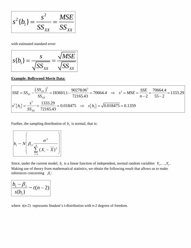
22
1{ }XX XX
s MSEs b
SS SS
with estimated standard error:
1{ }XX XX
s MSEs b
SS SS
Example: Bollywood Movie Data:
2 22
22
1 1
90278.06 70664.4183601.1 70664.4 1333.29
72165.43 2 55 2
1333.290.018475 0.018475 0.1359
72165.43
XY
YY
XX
XX
SS SSESSE SS s MSE
SS n
ss b s b
SS
Further, the sampling distribution of b1 is normal, that is:
b N
X Xii
n1 1
2
2
1
~ ,
( )
Since, under the current model, b1 is a linear function of independent, normal random variables nYY ,,1 .
Making use of theory from mathematical statistics, we obtain the following result that allows us to make
inferences concerning 1 :
)2(~}{ 1
11
ntbs
b
where t(n-2) represents Student’s t-distribution with n-2 degrees of freedom.
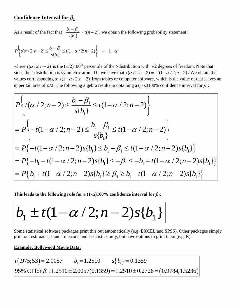
Confidence Interval for 1
As a result of the fact that )2(~}{ 1
11
ntbs
b , we obtain the following probability statement:
1 1
1
( / 2; 2) (1 / 2; 2) 1{ }
bP t n t n
s b
where )2;2/( nt is the (/2)100th
percentile of the t-distribution with n-2 degrees of freedom. Note that
since the t-distribution is symmetric around 0, we have that )2;2/1()2;2/( ntnt . We obtain the
values corresponding to )2;2/1( nt from tables or computer software, which is the value of that leaves an
upper tail area of /2. The following algebra results in obtaining a (1-)100% confidence interval for 1:
1 1
1
1 1
1
1 1 1 1
1 1 1 1 1
1 1
( / 2; 2) (1 / 2; 2){ }
(1 / 2; 2) (1 / 2; 2){ }
(1 / 2; 2) { } (1 / 2; 2) { }
(1 / 2; 2) { } (1 / 2; 2) { }
(1 / 2; 2) {
bP t n t n
s b
bP t n t n
s b
P t n s b b t n s b
P b t n s b b t n s b
P b t n s b
1 1 1} (1 / 2; 2) { }b t n s b
This leads to the following rule for a (1-)100% confidence interval for 1:
}{)2;2/1( 11 bsntb
Some statistical software packages print this out automatically (e.g. EXCEL and SPSS). Other packages simply
print out estimates, standard errors, and t-statistics only, but have options to print them (e.g. R).
Example: Bollywood Movie Data:
1 1
1
.975;53 2.0057 1.2510 0.1359
95% CI for :1.2510 2.0057(0.1359) 1.2510 0.2726 0.9784,1.5236
t b s b
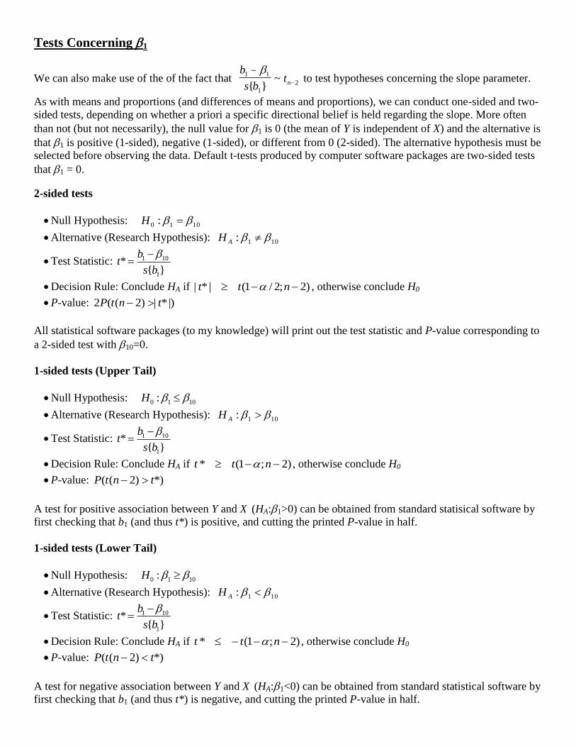
Tests Concerning 1
We can also make use of the of the fact that b
s btn
1 1
1
2
{ }~ to test hypotheses concerning the slope parameter.
As with means and proportions (and differences of means and proportions), we can conduct one-sided and two-
sided tests, depending on whether a priori a specific directional belief is held regarding the slope. More often
than not (but not necessarily), the null value for 1 is 0 (the mean of Y is independent of X) and the alternative is
that 1 is positive (1-sided), negative (1-sided), or different from 0 (2-sided). The alternative hypothesis must be
selected before observing the data. Default t-tests produced by computer software packages are two-sided tests
that 1 = 0.
2-sided tests
Null Hypothesis: 1010 : H
Alternative (Research Hypothesis): 101: AH
Test Statistic: 1 10
1
*{ }
bt
s b
Decision Rule: Conclude HA if )2;2/1(|*| ntt , otherwise conclude H0
P-value: |)*|)2((2 tntP
All statistical software packages (to my knowledge) will print out the test statistic and P-value corresponding to
a 2-sided test with 10=0.
1-sided tests (Upper Tail)
Null Hypothesis: 0 1 10:H
Alternative (Research Hypothesis): 101: AH
Test Statistic: 1 10
1
*{ }
bt
s b
Decision Rule: Conclude HA if )2;1(* ntt , otherwise conclude H0
P-value: *))2(( tntP
A test for positive association between Y and X (HA:1>0) can be obtained from standard statisical software by
first checking that b1 (and thus t*) is positive, and cutting the printed P-value in half.
1-sided tests (Lower Tail)
Null Hypothesis: 0 1 10:H
Alternative (Research Hypothesis): 101: AH
Test Statistic: 1 10
1
*{ }
bt
s b
Decision Rule: Conclude HA if )2;1(* ntt , otherwise conclude H0
P-value: *))2(( tntP
A test for negative association between Y and X (HA:1<0) can be obtained from standard statistical software by
first checking that b1 (and thus t*) is negative, and cutting the printed P-value in half.

Example: Bollywood Movie Data:
Question 1: Is there any association between Box Office Collection and Budget?
Question 2: Does increasing Budget by 1 unit lead to an increase in average Box Office Collection by > 1 unit?
1 1 2 2
0 1 1 0 1 1
*
1
*
2
Q1: : 0 : 0 Q2: : 0 : 0
1.2510 0TS1: 9.2035 .975;53 2.0057 Decision?
0.1359
value: 2 53 | 9.2035 | 0
1.2510 1TS2: 1.8469 .95;53 1.6741 Decision?
0.1359
value: 53 1.8
A AH H H H
t t
P P t
t t
P P t
469 .0352
Inferences Concerning 0
Recall that the least squares estimate of the intercept parameter, 0b , is a linear function of the observed
responses nYY ,,1 :
0 1
1 1
( )1n ni
i i i
i iXX
X X Xb Y b X Y l Y
n SS
Recalling that ii XYE 10}{ :
0 0 1 0 1
1 1 1
2
0 1 0 1 0
1 1
( ) ( ) ( )1 1 1{ } ( )
( )1(1 0) ( (1))
n n ni i i
i i
i i iXX XX XX
n ni
i
i i XX
X X X X X X X X XE b X X
n SS n SS n SS
X XX X X X
n SS
Thus, b0 is an unbiased estimator or the parameter 0.
Example: Bollywood Movie Data: 0 1 46.88 1.2510(39.04) 1.9549b Y b X
Below, we obtain the variance of the estimator of b0.

2 22
2 2 2
0 221 1
2 2
2 2 2
221 1
( ) ( ) 2 ( )1 1{ }
2 1( ) ( )
n ni i i
i iXX XXXX
n n
i i
i iXX XXXX
X X X X X X X X Xb
n SS n nSSSS
n X X XX X X X
n nSS n SSSS
Note that the variance will decrease as the sample size increases, as long as X values are not all placed at the
mean (which would not allow the regression to be fit). Further, the sampling distribution is normal under the
assumptions of the model. The estimated standard error of b0 replaces 2 with its unbiased estimate s
2=MSE and
taking the square root of the variance.
2 2
0
1 1{ }
XX XX
X Xs b s MSE
n SS n SS
Example: Bollywood Movie Data:
2
2
0
1333.29 55 39.04 72165.43
1 39.041333.29 52.40 7.24
55 72165.43
XXMSE s n X SS
s b
Note that )2(~}{ 0
00
ntbs
b , allowing for inferences concerning the intercept parameter 0 when it is
meaningful, namely when X=0 is within the range of observed data.
Confidence Interval for 0
Example: Bollywood Movie Data:
Although no movies have a budget of X=0, a 95% CI for 0 would be computed as follows:
}{)2;2/1( 00 bsntb
1.9549 2.0057(7.2385) 1.9549 14.5185 ( 16.47,12.56)

It is also useful to obtain the covariance of b0 and b1, as they are only independent under very rare
circumstances:
2 2
0 1
1 1 1 1
2 2 2 22
21 1
( ) ( )1{ , } , { }
( ) ( ) 0
n n n ni i
i i i i i i i
i i i i XX XX
n n
i i
i iXX XX XXXX
X X X X Xb b l Y k Y l k Y
n SS SS
X X XX X X X
nSS SS SSSS
In practice, X is usually positive, so that the intercept and slope estimators are usually negatively correlated.
We will use the result shortly.
Considerations on Making Inferences Concerning 0 and 1
Normality of Error Terms
If the data are approximately normal, simulation results have shown that using the t-distribution will provide
approximately correct significance levels and confidence coefficients for tests and confidence intervals,
respectively. Even if the distribution of the errors (and thus Y) is far from normal, in large samples the sampling
distributions of b0 and b1 have sampling distributions that are approximately normal as results of central limit
theorems. This is sometimes referred to as asymptotic normality.
Interpretations of Confidence Coefficients and Error Probabilities
Since X levels are treated as fixed constants, these refer to the case where we repeated the experiment many
times at the current set of X levels in this data set. In this sense, it’s easier to interpret these terms in controlled
experiments where the experimenter has set the levels of X (such as time and temperature in a laboratory type
setting) as opposed to observational studies, where nature determines the X levels, and we may not be able to
reproduce the same conditions repeatedly. This will be covered later.
Spacing of X Levels
The variances of b0 and b1 (for given n and 2) decrease as the X levels are more spread out, since their
variances are inversely related to 2
1
( )n
XX i
i
SS X X
. However, there are reasons to choose a diverse range of
X levels for assessing model fit. This is covered in Chapter 4.

Power of Tests
The power of a statistical test refers to the probability that we reject the null hypothesis. Note that when the null
hypothesis is true, the power is simply the probability of a Type I error (). When the null hypothesis is false,
the power is the probability that we correctly reject the null hypothesis, which is 1 minus the probability of a
Type II error (=1-), where denotes the power of the test and is the probability of a Type II error (failing to
reject the null hypothesis when the alternative hypothesis is true). The following procedure can be used to
obtain the power of the test concerning the slope parameter with a 2-sided alternative.
1) Write out null and alternative hypotheses: 1011010 :: AHH
2) Obtain the non-centrality measure, the standardized distance between the true value of 1 and the value
under the null hypothesis (10): }{ 1
101
b
3) Choose the probability of a Type I error (=0.05 or =0.01)
4) Determine the degrees of freedom for error: df = n-2
5) Using R, we can obtain the power as: Power = 1-pf(qf(1-,1,n-2),1,n-2,)
Note that the power increases as the non-centrality measure increases for a given degrees of freedom, and as the
degrees of freedom increases for a given non-centrality measure.
Confidence Interval for E{Yh}=0+1Xh
When we wish to estimate the mean at a hypothetical X value (within the range of observed X values), we can
use the fitted equation at that value of X=Xh as a point estimate, but we have to include the uncertainty in the
regression estimators to construct a confidence interval for the mean.
Parameter: hh XYE 10}{
Estimator: hh XbbY 10
^
We can obtain the variance of the estimator (as a function of X=Xh) as follows:
^
2 2 2 2 2
0 1 0 1 0 1
2 22 22 2 2
{ } { } 2 { , }
( )1 12
h h h h
hh h
XX XX XX XX
Y b b X b X b X b b
X XX XX X
n SS SS SS n SS

Estimated standard error of estimator:
n
i
i
hh
XX
XX
nMSEYs
1
2
2^
)(
)(1}{
Example: Bollywood Movie Data:
Suppose we are interested in mean Box Office Collection of all possible movies with budgets of Xh = 20
^
0 1
2
2^
20 1.9549 1.2510 1.9549 1.2510(20) 23.07
1333.29 55 20 39.04 72165.43
20 39.0411333.29 1333.29(0.02321) 30.94 5.56
55 72165.43
hh
h XX
h
X b b Y
MSE s n X X SS
s Y
)2(~
}{
}{^
^
nt
Ys
YEY
h
hh which can be used to construct confidence intervals for the mean response at specific X
levels, and tests concerning the mean (tests are rarely conducted).
(1-)100% Confidence Interval for E{Yh}:
}{)2;2/1(^^
hh YsntY
Example: Bollywood Movie Data:
23.07 2.0057(5.56) 23.07 11.15 (11.92,34.22)
Predicting a Future Observation When X is Known
If ,, 10 were known, we’d know that the distribution of responses when X=Xh is normal with mean
hX10 and standard deviation . Thus, making use of the normal distribution (and equivalently, the
empirical rule) we know that if we took a sample item from this distribution, it is very likely that the value will
fall within 2 standard deviations of the mean. That is, we would know that the probability that the sampled item
lies within the range 0 1 0 1( 2 , 2 )h hX X is approximately 0.95.

In practice, we don’t know the mean hX10 or the standard deviation . However, we have just
constructed a (1-)100% Confidence Interval for E{Yh}, and we have an estimate of (s). Intuitively, we can
approximately use the logic of the previous paragraph (with the estimate of ) across the range of believable
values for the mean. Then our prediction interval spans the lower tail of the normal curve centered at the lower
bound for the mean to the upper tail of the normal curve centered at the upper bound for the mean.
The prediction error for the new observation is the difference between the observed value and its predicted
value: hh YY^
. Since the data are assumed to be independent, the new (future) value is independent of its
predicted value, since it wasn’t used in the regression analysis. The variance of the prediction error can be
obtained as follows:
n
i
i
h
n
i
i
hhhhh
XX
XX
n
XX
XX
nYYYYpred
1
2
2
2
1
2
2
22^
22^
22
)(
)(11
)(
)(1}{}{}{}{
and an unbiased estimator is:
n
i
i
h
XX
XX
nMSEpreds
1
2
2
2
)(
)(11}{
Example: Bollywood Movie Data:
Suppose interested in predicting Box Office Collection of a single new movie with a budget of Xh = 20
^
0 1
2
2
20 1.9549 1.2510 1.9549 1.2510(20) 23.07
1333.29 55 20 39.04 72165.43
20 39.0411333.29 1 1333.29(1.02321) 1364.24 36.94
55 72165.43
hh
h XX
X b b Y
MSE s n X X SS
s pred

(1-)100% Prediction Interval for New Observation When X=Xh
n
i
i
hh
XX
XX
nMSEntY
1
2
2^
)(
)(11)2;2/(
Example: Bollywood Movie Data:
23.07 2.0057(36.94) 23.07 74.08 ( 51.01,97.15) (0,97.15)
Note: Unlike a Confidence Interval for a mean, which has a standard error that gets smaller, as the sample size
increases, the Prediction Interval for a single observation cannot be smaller than s, the residual standard
deviation. When that is large, prediction intervals will be wide, and often of little use.
It is a simple extension to obtain a prediction for the mean of m new observations when X=Xh. The sample mean
of m observations is m
2 and we get the following variance for the error in the prediction mean.
n
i
i
h
XX
XX
nmMSEpredmeans
1
2
2
2
)(
)(11}{
(1-)100% Prediction Interval for the Mean of m New Observations When X=Xh
n
i
i
hh
XX
XX
nmMSEntY
1
2
2^
)(
)(11)2;2/(
(1-)100% Confidence Band for the Entire Regression Line (Working-Hotelling Method)
)2,2;1(2}{^^
nFWYWsY hh

Example: Bollywood Movie Data:
2 0.95;2,55 2 2(3.1716) 2.5186W F
Selected values of Xh , estimates, standard errors, and half-widths for confidence band:
X_h Y-hat SE{Y-hat} W*SE{Yh}
5 4.30 6.82 17.18
20 23.06 5.38 13.55
40 48.08 5.07 12.78
60 73.10 6.76 17.02
80 98.12 9.42 23.73
100 123.14 12.45 31.35
-40.00
-20.00
0.00
20.00
40.00
60.00
80.00
100.00
120.00
140.00
160.00
180.00
0 20 40 60 80 100 120
Bo
x O
ffic
e C
olle
ctio
n
Budget
Working-Hotelling 95% Confidence Bands
Y-WSE
Y-hat
Y+WSE

Analysis of Variance Approach to Regression
0
50
100
150
200
250
300
0 20 40 60 80 100 120 140 160
Bo
x O
ffic
e C
olle
ctio
n
Budget
Observed Data, Fitted Line, Overall Mean
Y
Y-hat
Ybar
Consider the total deviations of the observed responses from the mean: YYi . When these terms are all
squared and summed up, this is referred to as the total sum of squares (SSTO).
n
i
i YYSSTO1
2)(
In the plot, these are the vertical distance of the points to the purple line just below 50. The more spread out the
observed data are, the larger SSTO will be.
Now consider the deviation of the observed responses from their fitted values based on the regression model:
iiiii eXbbYYY )( 10
^
. When these terms are squared and summed up, this is referred to as the error
sum of squares (SSE). We’ve already encountered this quantity and used it to estimate the error variance.
n
i
ii YYSSE1
2^
)(
When the observed responses fall close to the regression line, SSE will be small. When the data are not near the
line, SSE will be large.
Finally, there is a third quantity, representing the deviations of the predicted values from the mean. Then these
deviations are squared and summed up, this is referred to as the regression sum of squares (SSR).
n
i
i YYSSR1
2^
)(
The error and regression sums of squares sum to the total sum of squares: SSESSRSSTO which can be
seen as follows:

^ ^ ^ ^
^ ^ ^ ^ ^ ^2 2 2 2
^ ^ ^ ^2 2 2
1 1
^ ^ ^2 2
1 1
( ) ( )
( ) [( ) ( )] ( ) ( ) 2( )( )
( ) ( ) ( ) 2( )( )
( ) ( ) 2 (
i i i ii i i
i i i i i ii i i i
n n
i i i ii i i
i i
n n
i ii i
i i
Y Y Y Y Y Y Y Y Y Y
Y Y Y Y Y Y Y Y Y Y Y Y Y Y
SSTO Y Y Y Y Y Y Y Y Y Y
Y Y Y Y Y Y
^ ^ ^
2 2
0 1
1 1 1 1
^ ^ ^ ^2 2 2 2
0 1
1 1 1 1 1 1 1
^ ^2 2
1 1
)( ) ( ) ( ) 2 ( )
( ) ( ) 2 ( ) ( ) 2(0)
( ) ( )
n n n n
i i i ii i i
i i i i
n n n n n n n
i i i ii i i i i i
i i i i i i i
n n
i ii
i i
Y Y Y Y Y Y e b b X Y
Y Y Y Y b e b e X Y e Y Y Y Y
Y Y Y Y SSE SS
R
The last term was 0 since 0iii Xee ,
Each sum of squares has associated with degrees of freedom. The total degrees of freedom is dfT = n-1. The
error degrees of freedom is dfE = n-2. The regression degrees of freedom is dfR = 1. Note that the error and
regression degrees of freedom sum to the total degrees of freedom: )2(11 nn .
Mean squares are the sums of squares divided by their degrees of freedom:
21
n
SSEMSE
SSRMSR
Note that MSE was our estimate of the error variance, and that we don’t compute a total mean square. It can be
shown that the expected values of the mean squares are:
n
i
i XXMSREMSEE1
22
1
22 )(}{}{
Note that these expected mean squares are the same if and only if 1=0.
The Analysis of Variance is reported in tabular form:
Source df SS MS F
Regression 1 SSR MSR=SSR/1 F=MSR/MSE
Error n-2 SSE MSE=SSE/(n-2)
C Total n-1 SSTO
Example: Bollywood Movie Data:
2
1
22 2^
1
2 2^
1
Total: 183601.1 55 1 54
90278.6Error (Residual): 183601.1 70664.4 55 2 53
72165.43
9027Regression:
n
i YY TO
i
nXY
ii YY E
i XX
nXY
i
i XX
SSTO Y Y SS df
SSSSE Y Y SS df
SS
SSSSR Y Y
SS
28.6
112936.7 172165.43
Rdf

ANOVA Table:
ANOVA
df SS MS F
Regression 1 112936.7 112936.7 84.70529
Residual 53 70664.39 1333.29
Total 54 183601.1
F Test of 1 = 0 versus 1 0
As a result of Cochran’s Theorem (stated on page 76 of text book), we have a test of whether the dependent
variable Y is linearly related to the predictor variable X. This is a very specific case of the t-test described
previously. Its full utility will be seen when we consider multiple predictors. The test proceeds as follows:
Null hypothesis: 0: 10 H
Alternative (Research) Hypothesis: 0: 1 AH
Test Statistic: MSE
MSRFTS *:
Rejection Region: )2,1;1(*: nFFRR
P-value: *})2,1({ FnFP
Critical values of the F-distribution (indexed by numerator and denominator degrees’ of freedom) are given in
Table B.4, pages 1340-1345, and on class website, and can be obtained simply in EXCEL or R (see
Introduction). P-values must be obtained in EXCEL or R.
Note that this is a very specific version of the t-test regarding the slope parameter, specifically a 2-sided test of
whether the slope is 0. Mathematically, the tests are identical:
2
22
1
1
2
2
( )( )( )( )
( )( )0 1*{ }
( )
* *
i ii i XY
XY XX
ii XX
i
X X Y YX X Y Y SS SS SSX XX X SSb MSR
ts b MSE MSE MSE MSE MSE
X X
MSRt F
MSE
Further, the critical values are equivalent: )2,1;1())2;2/1(( 2 nFnt ,
check this from the two tables. Thus, the tests are equivalent.

Example: Bollywood Movie Data:
0 1 1: 0 : 0
112936.7Test Statistic: * 84.71 0.95;1,55 2 4.023
1333.29
value: (1,53) 84.71 .0000
AH H
MSRF F
MSE
P P F
Confirm the t-statistic, when squared, gives the F-statistic, and that the critical t-value for the 2-sided t-test is
the same as the critical F-value.
General Linear Test Approach
This is a very general method of testing hypotheses concerning regression models. We first consider the the
simple linear regression model, and testing whether Y is linearly associated with X. We wish to test 0: 10 H
vs 0: 1 AH .
Full Model
This is the model specified under the alternative hypothesis, also referred to as the unrestricted model. Under
simple linear regression with normal errors, we have:
iii XY 10
Using least squares (and maximum likelihood) to estimate the model parameters and the fitted values
( ii XbbY 10
^
), we obtain the error sum of squares for the full model:
SSEYYXbbYFSSE iiii
2^
2
10 )())(()(
Reduced Model
This the model specified by the null hypothesis, also referred to as the restricted model. Under simple linear
regression with normal errors, we have:
iiii XY 00 0
Using least squares (and maximum likelihood) to estimate the model parameter, we obtain Y as the estimate of
0, and have Yb 0 as the fitted value for each observation. We then obtain the following error sum of squares
under the reduced model:
SSTOYYbYRSSE ii
22
0 )()()(

Test Statistic
The error sum of squares for the full model will always be less than or equal to the error sum of squares for
reduced model, by definition of least squares. The test statistic will be:
F
FR
df
FSSE
dfdf
FSSERSSE
F)(
)()(
*
where FR dfdf , are the error degrees of freedom for the full and reduced
models. We will use this method throughout course.
For the simple linear regression model, we obtain the following quantities:
1)(2)( ndfSSTORSSEndfSSEFSSE RF
thus the F-Statistic for the General Linear Test can be written:
MSE
MSR
n
SSE
SSR
n
SSE
nn
SSESSTO
df
FSSE
dfdf
FSSERSSE
F
F
FR
2
1
2
)2()1(
)(
)()(
*
Thus, for this particular null hypothesis, the general linear test “generalizes” to the F-test.
Example: Bollywood Movie Data:
Suppose we wish to test whether on average, Box office collection is equal to the movie’s budget.
2
0 0 1
1
: 0, 1 ( ) 78593.4 55
( ) 70664.4 55 2 53
( ) ( ) 78593.4 70664.4
3964.555 53* 2.973 0.95;2,53 3.172 -value 0.0597( ) 70664.4 1333.3
53
n
i i R
i
F
R F
F
E Y X H SSE R Y X df n
SSE F df
SSE R SSE F
df dfF F P
SSE F
df
Descriptive Measures of Association
Along with the slope, Y-intercept, and error variance; several other measures are often reported.
Coefficient of Determination (r2)
The coefficient of determination measures the proportion of the variation in Y that is “explained” by the
regression on X. It is computed as the regression sum of squares divided by the total (corrected) sum of squares.
Values near 0 imply that the regression model has done little to “explain” variation in Y, while values near 1
imply that the model has “explained” a large portion of the variation in Y. If all the data fall exactly on the fitted
line, r2=1. The coefficient of determination will lie beween 0 and 1.

101 22 rSSTO
SSE
SSTO
SSRr
Coefficient of Correlation (r)
The coefficient of correlation is a measure of the strength of the linear association between Y and X. It will
always be the same sign as the slope estimate (b1), but it has several advantages:
In some applications, we cannot identify a clear dependent and independent variable, we just wish to
determine how two variables vary together in a population (peoples heights and weights, closing stock
prices of two firms, etc). Unlike the slope estimate, the coefficient of correlation does not depend on which
variable is labeled as Y, and which is labeled as X.
The slope estimate depends on the units of X and Y, while the correlation coefficient does not.
The slope estimate has no bound on its range of potential values. The correlation coefficient is bounded by –
1 and +1, with higher values (in absolute value) implying stronger linear association (it is not useful in
measuring nonlinear association which may exist, however).
11))((
))(()sgn( 1
2
1
rb
s
s
YYXX
YYXXrbr
y
x
ii
ii
where sgn(b1) is the sign (positive or negative) of b1, and yx ss , are the sample standard deviations of X and Y,
respectively.
Example: Bollywood Movie Data:
2 112936.70.6151
183601.1
90278.06.7843
72165.43(183601.1)
XY
XX YY
SSRr
SSTO
SSr
SS SS
Approximately 61.5% of the variation in box-office collection is “explained” by the film’s budget.

Tests Concerning the Population Correlation
Example: Bollywood Movie Data:
0 12 12
* 12
2
12
*
0
: 0 vs : 0 :
2 .7843 55 2Test Statistic: 9.204
1 .61511
Reject if 1 2 ; 2 .975,55 2 2.0057
AH H
r nt
r
H t t n t
(1-)100% Confidence Inteval for
1 2 1212
1 2 1 2
112 12
2 2
1 1
0 12
,Parameter:
Point (maximum likelihood) Estimator (aka Pearson product-moment correlation coefficient):
1 1
Testing :
n
i i
i XY
n nXX YY
i i
i i
Y Y
Y Y
X X Y YSS
r rSS SS
X X Y Y
H
12
* 12
2
12
*
0
*
12 0
*
12 0
0 vs : 0 :
2Test Statistic:
1
Reject if 1 2 ; 2
For 1-sided tests:
: 0 : Reject if 1 ; 2
: 0 : Reject if 1 ; 2
This test is mathematicall
A
A
A
H
r nt
r
H t t n
H H t t n
H H t t n
0 1y equivalent to t-test for : 0H
12 12
12
12
12
12
Problem: When 0, sampling distribution of is messy
11Fisher's z transformation: ' ln
2 1
11 1For large (typically at least 25): ' ~ , ln
3 2 1
Compute a
approx
r
rz
r
n z Nn
2
12 2
n approximate 1 100% CI for and transform back for :
11 100% CI for : ' 1 2
3
1After computing CI for , use identity
1
z zn
e
e

Example: Bollywood Movie Data:
12
12
2 2(0.7846)
12, 2 2(0.7
11 1 1 0.7843Fisher's z transformation: ' ln ln 1.0564
2 1 2 1 0.7843
11 100% CI for : ' 1 2
3
11.0564 1.96 1.0564 0.2718 (0.7846,1.3282)
55 2
1 1
1
LB
LBLB
rz
r
z zn
e e
e e
2 2(1.3282)
12, 2846) 2(1.3282)
1 10.6554 0.8688
1 1 1
95% CI for (0.6554,0.8688)
UB
UBUB
e e
e e
Issues in Applying Regression Analysis
When using regression to predict the future, the assumption is that the conditions are the same in future as
they are now. Clearly any future predictions of economic variables such as tourism made prior to September
11, 2001 would not be valid.
Often when we predict in the future, we must also predict X, as well as Y, especially when we aren’t
controlling the levels of X. Prediction intervals using methods described previously will be too narrow (that
is, they will overstate confidence levels).
Inferences should be made only within the range of X values used in the regression analysis. We have no
means of knowing whether a linear association continues outside the range observed. That is, we should not
extrapolate outside the range of X levels observed in experiment.
Even if we determine that X and Y are associated based on the t-test and/or F-test, we cannot conclude that
changes in X cause changes in Y. Finding an association is only one step in demonstrating a causal
relationship.
When multiple tests and/or confidence intervals are being made, we must adjust our confidence levels. This
is covered in Chapter 4.
When Xi is a random variable, and not being controlled, all methods described thus far hold, as long as the
Xi are independent, and their probability distribution does not depend on 2
10 ,, .