Systems & Control Letters 60 (2011) 832–839

Contents lists available at SciVerse ScienceDirect

Systems & Control Letters

journal homepage: www.elsevier.com/locate/sysconle

Stability analysis for time-varying systems via quadratic constraints✩

Liu Liu ∗, YuFeng LuSchool of Mathematical Sciences, Dalian University of Technology, Dalian 116024, China

a r t i c l e i n f o

Article history:Received 27 December 2010Accepted 13 June 2011Available online 16 August 2011

Keywords:StabilityQuadratic constraintCompletely finiteNest algebraConnected uncertainty setGap metricTime-varying system

a b s t r a c t

In this paper, we introduce the concept of ‘‘quadratic constraint’’ (QC) to deal with various stabilityproblems for infinite dimensional linear discrete time-varying (LTV) systems. First, we derive a necessaryand sufficient condition for the close-loop stability based on quadratic constraints (QCs). An equivalentcondition of this stability criterion presents the relationship between the stabilization of each finitedimensional truncation system and that of the whole system. Moreover, applying this stability criterionand the complete finiteness of the nest algebra, we show that the plant is stabilizable if and only if it has asingle strong representation. Finally, we use QCs to give a necessary and sufficient condition for the robuststabilization of connected uncertainty set defined by gap metric.

© 2011 Elsevier B.V. All rights reserved.

1. Introduction

The integral quadratic constrains (IQCs) technique was origi-nally developed in a robust control framework and has become oneof the powerfulmethods for system analysis. A large variety of con-trol results were recently unified and generalized using the notionof IQC. In the 1970’s, Yakubovich used IQCs to solve the stabilityproblems in H∞ control. Later on, Safonov interpreted the stabil-ity results in terms of separation of the graphs of the two systemsin the closed-loop, which is an energy-related interpretation. Dur-ing the last decade, a variety of methods about robust control havebeen developed, many of which can be reformulated within theframework of IQCs (see [1–4]).

The stability of standard feedback configuration with the plantL and the compensator C has been studied in various frameworks.The common point of reference is that the feedback stabilityis equivalent to that the direct sum of signal spaces can bedecomposed as the algebraic direct sum of the graph of L and theinverse graph of C (see [5,6]). In 1980 Zames and El Sakkary definedthe gap metric on possibly unstable but stabilizable systems basedon the graphs of the systems [7]. Later on, the stability criterion interms of the gap metric was originally established by El-Sakkaryin [8]. After that, the gapmetric became a powerful tool for solving

✩ This research is supported by NSFC, Item Number: 10971020.∗ Corresponding author. Tel.: +86 0411 84708352; fax: +86 0411 84708352.

E-mail addresses: beth.liu@yahoo.com.cn (L. Liu), lyfdlut1@yahoo.com.cn(Y. Lu).

0167-6911/$ – see front matter© 2011 Elsevier B.V. All rights reserved.doi:10.1016/j.sysconle.2011.06.007

feedback stability and robust stabilizing problems (see [9–12]). In1997,Megresky andRantzer presented a classical stability theoremfor systems described by IQCs in [1]. Using the KYP lemma, the IQCsrelated to the stability can be transferred to LMIs. This criterion hasreceived much attention in connection to the robust H∞ controlproblem, but the IQCs theory only offers sufficient conditions forstability. Recently, a necessary and sufficient condition for robuststability of a class of special interconnected systems was derivedin [2].

Many methods have been used to recognize and discuss theclosed-loop stability of causal LTV systems in the framework ofnest algebras, such as graph theory, coprime factorization theoryand gap metric theory [5]. Here we bring out the definition of QCsto discuss the stability. To the best of our knowledge, there are nocorresponding results in the literature for closed-loop stability inthe framework of nest algebra.

The purpose of this paper is to characterize various stabilityproblems for discrete time LTV systems in terms of QCs, anduse the new results about nest algebra to get a necessary andsufficient condition for the stabilization. The approach taken hereis the input–output approach, where the systems are thoughtof as linear (possibly unbounded) operators. We prove that thestability of closed-loop system is equivalent to that the orthogonalcomplements of the two graphs for the plant and compensatorsatisfy a corresponding pair of complementary QCs. The QCsrelated to the stability can also be transferred to LMIs, which canbe calculated by the YALMIP tool-box in Matlab. In [5], Feintuchpointed out that the plant is stabilizable if and only if it has a doublecoprime factorization. Indeed, the algebra of stable LTV systemsconsidered here is a maximal nest algebra. We use the QC stability

L. Liu, Y. Lu / Systems & Control Letters 60 (2011) 832–839 833

criterion and the complete finiteness of the nest algebra to showthat the plant is stabilizable if and only if it has a single coprimefactorization. We also use the QCs theory to solve a type of robuststability problem, in which the uncertainty set is a connected setdefined by gap metric.

This paper is organized as follows. In Section 2, we give somenotations, definitions and auxiliary propositions. In Section 3, wegive some necessary and sufficient conditions for the closed-loopstability. Sections 4 and 5 are devoted to give a simulation andapplications for the stability criterion. In Section 6, we provethat the plant is stabilizable if and only if it has a single strongrepresentation. In the last section, we consider the robust stabilitybased on QCs.

2. Preliminaries

Let ℓ2= {(x0, x1, . . .) :

∑∞

i=0 |xi|2 < ∞, xi ∈ C} be the input–output space. The inner product and the norm on ℓ2 are definedrespectively, by

⟨x, y⟩ =

∞−i=0

xiyi, ‖x‖2= ⟨x, x⟩

12 .

ℓ2 is a complex separate Hilbert space, and let ℓ2e = {(x0, x1, . . .) :

xi ∈ C} be the extended space of ℓ2.Let ℓ2

⊕ℓ2=

xy

: x, y ∈ ℓ2

be a Hilbert spacewith the inner

product defined by[x1y1

],

[x2y2

]= ⟨x1, x2⟩ℓ2 + ⟨y1, y2⟩ℓ2 ,[

xiyi

]∈ ℓ2

⊕ ℓ2, i = 1, 2.

Let B(H) denote the space of bounded linear operators onHilbert space H and T ∈ B(H). The adjoint of T , denoted as T ∗, isdefined by ⟨T ∗x, y⟩ = ⟨x, Ty⟩, ∀x, y ∈ H . T is self-adjoint if T = T ∗.A self-adjoint operator T is positive, denoted T ≥ 0, if ⟨Tx, x⟩ ≥ 0for all x ∈ H . It is strictly positive (T > 0) if there exists ε > 0such that ⟨Tx, x⟩ ≥ ε‖x‖2 for all x ∈ H . Similarly, T ≤ 0 and T < 0can be defined. The operator norm of T is ‖T‖ = supx∈H,‖x‖≤1 ‖Tx‖.

The truncation projection Pn on ℓ2 and ℓ2e will be defined by

Pn(x0, x1, . . . , xn, . . .) = (x0, x1, . . . , xn, 0, . . .), n ≥ 0.

Denote P−1 = 0 and P∞ = I .{Pn : −1 ≤ n ≤ ∞} is used to define the physical definition of

causality. A linear transformation L on ℓ2e is causal if PnLPn = PnL

for all −1 ≤ n ≤ ∞. A linear system on ℓ2e is a causal linear

transformation on ℓ2e , which is continuous with respect to the

resolution topology. A linear system L is stable if its restriction toℓ2 is a bounded operator (see [5]).

Let L be the algebra of linear systems with respect to thestandard addition and multiplication. It is easy to check that anyelement in L is a lower triangular matrix with respect to standardbasis. The set of stable ones, denoted by S, is a weakly closedalgebra containing the identity, referred to in the operator theoryliterature as a nest algebra. Denote

M2(S) =

[S11 S12S21 S22

]: Sij ∈ S, i, j = 1, 2.

.

Anest is a chainN of closed subspaces of aHilbertH containing{0} and H which is closed under intersection and closed span. Thenest algebra determined by N is

T (N ) = {T ∈ B(H) : TN ⊆ N, ∀N ∈ N }.

Indeed, S is the nest algebra determined by the nest {I−Pn : −1 ≤

n ≤ ∞}.

Definition 2.1 ([5]). Suppose T is a linear operator defined onD(T ) ⊆ H , where D(T ) = {x ∈ H : Tx ∈ H}. The graph of T ,denoted G(T ), is the set

xTx

: x ∈ D(T )

⊆ H ⊕ H . The inverse

graph of T is G−1(T ) =

TI

D(T ). T is a closed if G(T ) is a closed

subspace of H ⊕ H .

Theorem 5.3.4 in [5] tells us that any L ∈ L is a closed operator.In order to character the stability, we need the definitions of

strong representations for linear systems.

Definition 2.2 ([5]). (a).MN

is a strong right representation of

L ∈ L if

1. M,N ∈ S and there exist X, Y ∈ S such that [Y X]

MN

= I,

2. G(L) = RanMN

.

MN

is normalized if it is an isometry.

(b). [−N M] is a strong left representation of L ∈ L if

1. N, M ∈ S and there exist X, Y ∈ S such that [−N M]

XY

= I,

2. G(L) = Ker[−N M].

[−N M] is normalized if it is a co-isometry.

If L has a strong representation, it must have a normalizedstrong representation (Ch6, [5]).

Theorem 2.1 ([5]). Suppose M,N ∈ S. ThenMN

is a strong right

representation for L ∈ L if and only if

1. there exist X, Y ∈ S such that [Y X]MN

= I ,

2. M is invertible in L.

The proof of Theorem 2.1 implies thatMN

is a strong right

representation of L if and only if NM−1 is a right coprimefactorization of L. Similarly, [−N M] is a strong left representationof L if and only if M−1N is a left coprime factorization of L.

Lemma 2.1 ([5]). Suppose A, B, X, Y ∈ S such that XA + YB = I ,then there exists Q ∈ S such that A + QB is invertible in L.

Definition 2.3 ([5]). Let M1 and M2 be closed subspaces of H ,and PM1 , PM2 denote the corresponding orthogonal projections,respectively. The directed gap from M1 to M2 is

−→δ (M1, M2)

= ‖PM⊥2PM1‖, and the gap between M1 and M2 is δ(M1, M2) =

max{−→δ (M1, M2),

−→δ (M2, M1)}.

Theorem 2.2. If δ(M1, M2) < 1, then δ(M1, M2) =−→δ (M1, M2)

=−→δ (M2, M1).

For closed operators L1, L2, δ(L1, L2) denotes the gap betweenG(L1)and G(L2).

In this paper,we consider stability of the feedback configurationwith the plant L and the compensator C . L and C are two linearsystems, and the close loop equation is[e1e2

]=

[I CL I

] [u1u2

].

The closed loop system {L, C} is well-posed if each entry of theoperator matrix from external input e =

e1e2

to internal input

u =

u1u2

is causal, and it is stable if[

I CL I

]−1

=

[(I − CL)−1 C(I − LC)−1

−L(I − CL)−1 (I − LC)−1

]∈ M2(S).

834 L. Liu, Y. Lu / Systems & Control Letters 60 (2011) 832–839

A linear system L is stabilizable if there exists C ∈ L suchthat the closed-loop {L, C} is stable. The following theorem is theclassical Youla Parametrization Theorem.

Theorem 2.3 ([5]). A linear system L ∈ L is stabilizable if and only ifL has a strong right and a strong left representation. If this is the casethe representations can be chosen so that we have the double Bezoutidentity[

Y −X−N M

] [M XN Y

]=

[M XN Y

] [Y −X

−N M

].

A causal linear system C stabilizes L if and only if it has a strong

right representationY + NQX + MQ

and a strong left representation [−(X−

QM) Y − QN] for some Q ∈ S.

3. Stability of closed-loop system

In this section, we introduce QCs to character the stability ofthe closed-loop system {L, C}. Feintuch presented many familiarnecessary and sufficient conditions for the closed-loop stability ofinfinite-dimensional LTV discrete time systems in [5] and we listall in the following.

Theorem 3.1 ([5]). Suppose L and C ∈ L are stabilizable with strongrepresentations

MN

, [−N M] for L and

VU

, [−U V ] for C. The

following statements are equivalent:

a. {L, C} is stable.b. G(L) + G−1(C) = ℓ2

⊕ ℓ2.

c.

V −U−N M

is invertible on ℓ2

⊕ ℓ2.

d.M UN V

is invertible on ℓ2

⊕ ℓ2.

e. MV − NU is invertible in S.f. VM − UN is invertible in S.g. δ(G−1(C)⊥, G(L)) =

PG(L)⊥PG−1(C)⊥

< 1.h. The parallel projection onto G−1(C)⊥ along G(L), denoted by

PG−1(C)⊥ |G(L), is invertible.

Remark 3.1. In fact, {L, C} is stable if and only ifI CL I

is a one

to one and onto operator from D(L) ⊕ D(C) to ℓ2× ℓ2. This is

equivalent to G(L) ∩ G−1(C) = {0} and G(L) + G−1(C) = ℓ2× ℓ2.

But in our background, we have the fact that ‘‘If T ∈ S is onto,then T is invertible in S’’. Based on this result, Feintuch proved thatG(L) + G−1(C) = ℓ2

× ℓ2 is equivalent to the closed-loop stability.Likewise, in general, {L, C} is stable if and only if

δ(G−1(C)⊥, G(L))= max

PG(L)⊥PG−1(C)⊥

,PG(L)PG−1(C)

< 1.

Here, we just need the condition that the directed gap ‖PG(L)⊥

PG−1(C)⊥‖ < 1.Moreover, we have thatPG(L)PG−1(C)

≤PG(L)⊥PG−1(C)⊥

(3.1)

holds for any L, C ∈ L.

Many versions of integral quadratic constraints are availablefor the particular application in time invariant systems. Now, weintroduce the definitions of quadratic constraint about the signalsand the signal set to deal with the stability of the time-varyingsystems.

Definition 3.1. Two signals x, y ∈ ℓ2 satisfy the quadratic con-straint determined by Φ = Φ∗

∈ B(ℓ2× ℓ2) if

Φ

xy

,xy

≥ 0.

LetW ⊆ ℓ2×ℓ2 be a signal set.W is said to satisfy the quadratic

constraint determined by Φ = Φ∗∈ B(ℓ2

× ℓ2), denoted byW ∈ QC(Φ), if

⟨Φw, w⟩ ≥ 0, w ∈ W .

Likewise, W satisfies the strict quadratic constrain determined byΦ , denoted by W ∈ SQC(Φ) if there exists ε > 0 such that

⟨Φw, w⟩ ≥ ε‖w‖2, w ∈ W .

On system analysis, we use the quadratic constraints aboutG(L)⊥ and G(C)⊥ to describe the stability of closed-loop {L, C}.

The following proposition shows that QCs in systems can bedescribed in the form of operator inequalities corresponding withstrong representations.

Proposition 3.1. LetMN

be a strong right representation of L and

−N Mbe a strong left representation of L. Then the following

statements hold:

a. G(L) ∈ QC(Φ) if and only if [M∗ N∗]Φ

MN

≥ 0.

b. G(L)⊥ ∈ QC(Φ) if and only if−N M

Φ

−N∗

M∗

≥ 0.

c. G−1(L) ∈ QC(Φ) if and only if [N∗ M∗]Φ

NM

≥ 0.

d. G−1(L)⊥ ∈ QC(Φ) if and only if [M − N]Φ

M∗

−N∗

≥ 0.

Similarly, the strict quadratic constraints are equivalent to thestrict operator equalities.

Proof. Only (b) in the strict quadratic constraintwill be shown andthe others are analogous.

b. Since G(L) = Ker−N M

=

Ran

−N∗

M∗

⊥

, we have

G(L)⊥ = Ran−N∗

M∗

. Since

−N M

is right invertible, hence

−N∗

M∗

is left invertible. Therefore,

G(L)⊥ = Ran[−N∗

M∗

],

and there exist K1 > 0 and K2 > 0 such that

K1‖x‖ ≤

[−N∗

M∗

]x ≤ K2‖x‖, x ∈ ℓ2.

Suppose G(L)⊥ ∈ SQC(Φ), this means thatΦ

−N∗

M∗

x,

−N∗

M∗

x

≥ ε1

−N∗

M∗

x2

holds for some ε1 > 0. ThenΦ

−N∗

M∗

x,

−N∗

M∗

x

≥ K12ε‖x‖2, x ∈ ℓ2.

Turn to the other direction. Assume that−N M

Φ

−N∗

M∗

> 0 is known. Hence there exists ε2 > 0 such that

Φ

[−N∗

M∗

]x,

[−N∗

M∗

]x

≥ ε2‖x‖2

≥ε2

K 22

[−N∗

M∗

]x2

, x ∈ ℓ2.

That is G(L)⊥ ∈ SQC(Φ). �

L. Liu, Y. Lu / Systems & Control Letters 60 (2011) 832–839 835

Remark 3.2. From the proof of Proposition 3.1, we obtain the fact

that G(L)⊥ = Ran−N∗

M∗

and G−1(C)⊥ = Ran

V∗

−U∗

. The directed

gap metric can be written asPG(L)⊥PG−1(C)⊥

= ‖UM∗+ V N∗

‖, (3.2)PG(L)PG−1(C)

= ‖UM∗+ VN∗

‖, (3.3)

whereMN

and

−N M

are the normalized strong right and left

representation of L respectively, andUV

,−U V

be the same

for C .

In the rest of this section, wewill show that the interconnectionsystem {L, C} is stable if and only if G(L)⊥ and G−1(C)⊥ satisfy acorresponding pair of complementary QCs.

Theorem 3.2. If linear systems L and C have strong left representa-tions, then the closed-loop system {L, C} is stable if and only if thereexists a Φ = Φ∗

∈ B(ℓ2× ℓ2) such that G(L)⊥ ∈ SQC(Φ) and

G−1(C)⊥ ∈ QC(−Φ).

Proof. ‘‘⇐’’ Suppose G−1(C)⊥ ∈ QC(−Φ) and G(L)⊥ ∈ SQC(Φ).We have ⟨Φv, v⟩ ≤ 0 for all v ∈ G−1(C)⊥, and there exists ϵ > 0such that ⟨Φw, w⟩ ≥ ϵ‖w‖

2 for all w ∈ G(L)⊥. It follows that

ϵ‖w‖2

≤ ⟨Φw, w⟩ − ⟨Φv, v⟩

= −⟨Φ(w + v), w + v⟩ + 2Re⟨Φ(w + v), w⟩

≤ ‖Φ‖ · ‖w + v‖2+ 2‖Φ‖ · ‖w + v‖ · ‖w‖

≤ ‖Φ‖ · ‖w + v‖2+

2‖Φ‖2· ‖w + v‖

2

ϵ+

ϵ

2‖w‖

2.

Thus

‖w + v‖2

≥ η‖w‖2, w ∈ G(L)⊥, v ∈ G−1(C)⊥, (3.4)

where η =ϵ2

2ϵ‖Φ‖+4‖Φ‖2. Since ‖Φ‖ ≥ ϵ, it is easy to see that

0 < η < 16 .

Let−N M

be normalized strong left representation for L,

and−U V

be the same for C . For all x ∈ ℓ2 with ‖x‖ = 1,

from Remark 3.2, we have−N∗

M∗

x ∈ G(L)⊥ and −

V∗

−U∗

(UM∗

+

V N∗)x ∈ G−1(C)⊥. Note (3.4), we get

η ≤

[−N∗

M∗

]x −

[V ∗

−U∗

](UM∗

+ V N∗)x2

=

I −

[V ∗

−U∗

] V −U

[−N∗

M∗

]x2

=

[−N∗

M∗

]x2

−

[V ∗

−U∗

] V −U

[−N∗

M∗

]x2

= 1 − ‖(UM∗+ V N∗)x‖2.

Since the arbitrary of x, we have ‖UM∗+ V N∗

‖ ≤ 1 − η < 1,that is

PG(L)⊥PG−1(C)⊥

< 1. From Theorem 2.1, we obtain that theclosed-loop {L, C} is stable. ‘‘⇒’’ If {L, C} is stable, by Theorem 3.1,there exists

S11 S12S21 S22

∈ B(ℓ2

× ℓ2) such that[V −U

−N M

] [S11 S12S21 S22

]= I.

This implies that−N M

[S12S22

][S∗

12 S∗

22]

[−N∗

M∗

]= I, (3.5)

andV −U

[S12S22

][S∗

12 S∗

22]

[V ∗

−U∗

]= 0. (3.6)

From Proposition 3.1, (3.5) and (3.6) are equivalent to G(L)⊥ ∈

SQC(Φ) and G−1(C)⊥ ∈ QC(−Φ) respectively, where Φ =S12S22

[S∗

12 S∗

22]. The proof is completed. �

The following theorem is the dual form of Theorem 3.2.

Theorem 3.3. If linear systems L and C have strong left representa-tions, then the closed-loop system {L, C} is stable if and only if thereexists a Φ = Φ∗

∈ B(ℓ2× ℓ2) such that G(L)⊥ ∈ QC(Φ) and

G−1(C)⊥ ∈ SQC(−Φ).

Theorems 3.2 and 3.3 mean that the closed-loop system {L, C}

is stable if and only if G(L)⊥ and G−1(C)⊥ satisfy the coupled QCs.Using Proposition 3.1, the conditions can bewritten in terms of theseparation of the strong representations for the two systems in thefeedback configuration, which are two operator inequalities. Fromanother view, the stability of {L, C} is related to the existence ofsolution for two coupled operator inequalities, which we presentin the following theorem.

Theorem 3.4. If L and C have strong left representations−N M

and

−U V

, respectively, then the closed-loop system {L, C} is

stable if and only if the inequalities−N M

Φ

[−N∗

M∗

]> 0

V −U

Φ

[V ∗

−U∗

]≤ 0

have a self-adjoint solution Φ ∈ B(ℓ2× ℓ2).

Corollary 3.1. Assume L ∈ S and C ∈ S. If there exists ∆ ∈ B(H)such that

L∆ + ∆∗L∗ > 0, C∆∗+ ∆C∗

≤ 0,

then {L, C} is stable.

Proof. Since L ∈ S and C ∈ S, thus [−L I] and [−C I] arestrong left representations for L and C respectively. Set Φ =

0 −∆

−∆∗ 0

, then the proof will be completed by applying

Theorem 3.4. �

Wewill give a new stability criterion based on LMIs, which canbe realized by a computer.

Note that Pnℓ2= {(x0, x1, . . . , xn, 0, . . .) : xi ∈ C} is isomor-

phic to Cn. In the following theorem, we use Pn to denote both thetruncation on ℓ2 and the identity matrix in Cn×n without distin-guishing between them.

Theorem 3.5. If L and C have strong left representations, thenthe closed-loop system {L, C} is stable if and only if the followingconditions hold:

For any n ≥ 0, the LMIs

[−PnL Pn]Φn

[−(PnL)∗

Pn

]− PnL(PnL)∗ − Pn ≥ 0 (3.7)

and

[Pn − PnC]Φn

[Pn

−(PnC)∗

]≤ 0 (3.8)

have a self-adjoint solution Φn ∈ C2n×2n such that supn≥0 ‖Φn‖

< +∞.

836 L. Liu, Y. Lu / Systems & Control Letters 60 (2011) 832–839

Proof. ‘‘⇐’’ Let−N M

be strong left representations for L.

Since PnL = PnM−1PnN , we have

Ran[−(PnL)∗

Pn

]= Ran

[−(PnN)∗

(PnM)∗

](PnM−1)∗ = Ran

[−N∗

M∗

]Pn.

So (3.7) is equivalent toΦn

[−N∗

M∗

]Pnx,

[−N∗

M∗

]Pnx

≥

[−N∗

M∗

]Pnx

2

, x ∈ ℓ2. (3.9)

Similarly, let−U V

be strong left representations for C . (3.8) is

equivalent toΦn

[V ∗

−U∗

]Pny,

[V ∗

−U∗

]Pny

≤ 0, y ∈ ℓ2. (3.10)

As the proof of Theorem 3.2, (3.9) and (3.10) imply that[−N∗

M∗

]Pnx +

[V ∗

−U∗

]Pny

2

≥ ηn

[−N∗

M∗

]Pnx

2

,

x ∈ ℓ2, y ∈ ℓ2, (3.11)

where ηn =1

2‖Φn‖+4‖Φn‖2. Since 1 ≤ ‖Φn‖ ≤ supn≥0 ‖Φn‖, we get

12 supn≥0 ‖Φn‖+4 supn≥0 ‖Φn‖2

≤ ηn ≤16 for all n ≥ 0. Thus[

−N∗

M∗

]Pnx +

[V ∗

−U∗

]Pny

2

≥ r[

−N∗

M∗

]Pnx

2

, x ∈ ℓ2, y ∈ ℓ2,

where 0 < r =1

2 supn≥0 ‖Φn‖+4 supn≥0 ‖Φn‖2< 1. Therefore

−N∗

M∗

x +

V∗

−U∗

y2

≥ r

−N∗

M∗

x2

, x ∈ ℓ2, y ∈ ℓ2, valid forPn converging to I in the strong operator topology. Following theproof of Theorem 3.2, we obtain that the closed-loop system {L, C}

is stable.‘‘⇒’’ Suppose {L, C} is stable, from Theorem 3.4, there exist a

self-adjoint operator Φ ∈ B(ℓ2× ℓ2) and β > 0 such that

−N M

Φ

[−N∗

M∗

]≥ β

−N M

[−N∗

M∗

](3.12)

andV −U

Φ

[V ∗

−U∗

]≤ 0. (3.13)

The operator Φ can be decomposed in the formΦ11 Φ12Φ21 Φ22

, where

Φij ∈ B(ℓ2), i, j = 1, 2. Set

Φn =1β

[PnΦ11Pn PnΦ12PnPnΦ21Pn PnΦ22Pn

]∈ C2n×2n,

where PnΦijPn denotes the n × nmatrix which is the truncation ofΦij restricted on Cn. Hence supn≥0 ‖Φn‖ ≤

1β‖Φ‖ < +∞. Since

the causality, (3.12) and (3.13) imply that

1βPn

−N M

Φn

[−N∗

M∗

]Pn ≥ Pn

−N M

[−N∗

M∗

]Pn, (3.14)

and

PnV −U

Φn

[V ∗

−U∗

]Pn ≤ 0. (3.15)

From the fact that Ran−(PnL)∗

Pn

= Ran

−N∗

M∗

Pn and Ran

Pn

−(PnC)∗

= Ran

V∗

−U∗

Pn, we have that (3.14) and (3.15) are equivalent to

(3.7) and (3.8) respectively. �

Remark 3.3. Theorem 3.5 clearly describes the relationship be-tween the stabilization of L and that of the truncation system PnL.If there exists a truncation system Pn0L is not stabilizable, then lin-ear system L can not be stabilized. However, we can not obtain thestabilization of L even if PnL is stabilizable for all n. For instance,

L =

01 0

2 0. . .

. . .

is not stabilizable (see Example 6.2.2 in [5]).

But for any n ≥ 0, PnL is stabilizable.

4. Simulation

In this section, we present an example to demonstratethe effectiveness and applicability of the proposed method inTheorem 3.5.

Consider the plant L =

11 21 2 31 2 0 4...

.

.

....

.

.

.. . .

.

Let

C1 =

01 0

2 0. . .

. . .

and C2 =

−1

−2−3

. . .

.

The LMIs in Theorem 3.5 can be solved by using Matlab (withYALMIP toolbox [13]), then the stability can be obtained from thesolvability of LMIs. Design a linear objectiveminimization problemunder LMI constraints and the output is the solution of LMIs whichhas the minimal norm.

First consider the closed-loop system {L, C1}.n = 2,

Φ2 =

0.5762 −0.2128 −1.1143 −1.4938−0.2128 0.0471 1.0607 −1.5317−1.1143 1.0607 0.6640 0.6960−1.4938 −1.5317 0.6960 0.24660

with ‖Φ2‖ = 2.3453.

n = 3,

Φ3 =

−4.2411 1.0626 −2.7031 −4.7968 −2.5468 −10.33941.0626 2.2791 −0.9749 6.6110 −3.9828 −7.2479

−2.7031 −0.9749 4.9864 2.2223 6.4529 −4.0297−4.7968 6.6110 2.2223 1.1147 0.0437 6.7933−2.5468 −3.9828 6.4529 0.0437 −4.7326 2.2831−10.3394 −7.2479 −4.0297 6.7933 2.2831 0.8395

with ‖Φ3‖ = 15.5868.

The best objective values:

n = 6, ‖Φ6‖ = 1.0957e + 005,n = 7, ‖Φ7‖ = 4.5837e + 006,n = 8, ‖Φ8‖ = 2.5608e + 008.

For n = 9, the LMI constraints were found INFEASIBLE. That is, forn = 9, the LMIs (3.7) and (3.8) are unsolved. Thus {L, C1} is notstable.

Note the simulation above, although the LMIs have solutionswhen n ≤ 8, the normofwhich increases substantially as the valueof n increases.

L. Liu, Y. Lu / Systems & Control Letters 60 (2011) 832–839 837

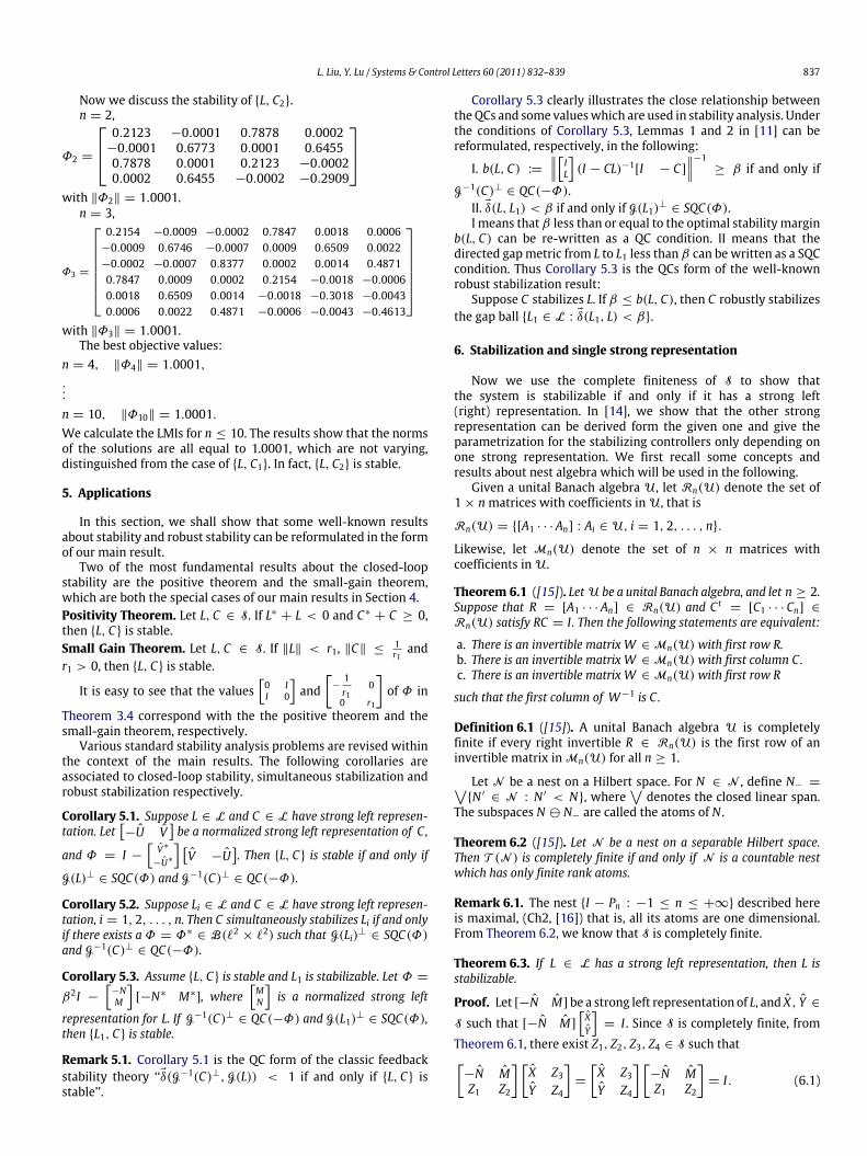
Now we discuss the stability of {L, C2}.n = 2,

Φ2 =

0.2123 −0.0001 0.7878 0.0002−0.0001 0.6773 0.0001 0.64550.7878 0.0001 0.2123 −0.00020.0002 0.6455 −0.0002 −0.2909

with ‖Φ2‖ = 1.0001.

n = 3,

Φ3 =

0.2154 −0.0009 −0.0002 0.7847 0.0018 0.0006−0.0009 0.6746 −0.0007 0.0009 0.6509 0.0022−0.0002 −0.0007 0.8377 0.0002 0.0014 0.48710.7847 0.0009 0.0002 0.2154 −0.0018 −0.00060.0018 0.6509 0.0014 −0.0018 −0.3018 −0.00430.0006 0.0022 0.4871 −0.0006 −0.0043 −0.4613

with ‖Φ3‖ = 1.0001.

The best objective values:n = 4, ‖Φ4‖ = 1.0001,...

n = 10, ‖Φ10‖ = 1.0001.We calculate the LMIs for n ≤ 10. The results show that the normsof the solutions are all equal to 1.0001, which are not varying,distinguished from the case of {L, C1}. In fact, {L, C2} is stable.

5. Applications

In this section, we shall show that some well-known resultsabout stability and robust stability can be reformulated in the formof our main result.

Two of the most fundamental results about the closed-loopstability are the positive theorem and the small-gain theorem,which are both the special cases of our main results in Section 4.Positivity Theorem. Let L, C ∈ S. If L∗

+ L < 0 and C∗+ C ≥ 0,

then {L, C} is stable.Small Gain Theorem. Let L, C ∈ S. If ‖L‖ < r1, ‖C‖ ≤

1r1

andr1 > 0, then {L, C} is stable.

It is easy to see that the values0 II 0

and

[−

1r1

0

0 r1

]of Φ in

Theorem 3.4 correspond with the the positive theorem and thesmall-gain theorem, respectively.

Various standard stability analysis problems are revised withinthe context of the main results. The following corollaries areassociated to closed-loop stability, simultaneous stabilization androbust stabilization respectively.

Corollary 5.1. Suppose L ∈ L and C ∈ L have strong left represen-tation. Let

−U V

be a normalized strong left representation of C,

and Φ = I −

V∗

−U∗

V −U

. Then {L, C} is stable if and only if

G(L)⊥ ∈ SQC(Φ) and G−1(C)⊥ ∈ QC(−Φ).

Corollary 5.2. Suppose Li ∈ L and C ∈ L have strong left represen-tation, i = 1, 2, . . . , n. Then C simultaneously stabilizes Li if and onlyif there exists a Φ = Φ∗

∈ B(ℓ2× ℓ2) such that G(Li)⊥ ∈ SQC(Φ)

and G−1(C)⊥ ∈ QC(−Φ).

Corollary 5.3. Assume {L, C} is stable and L1 is stabilizable. Let Φ =

β2I −

−NM

[−N∗ M∗

], whereMN

is a normalized strong left

representation for L. If G−1(C)⊥ ∈ QC(−Φ) and G(L1)⊥ ∈ SQC(Φ),then {L1, C} is stable.

Remark 5.1. Corollary 5.1 is the QC form of the classic feedbackstability theory ‘‘δ(G−1(C)⊥, G(L)) < 1 if and only if {L, C} isstable’’.

Corollary 5.3 clearly illustrates the close relationship betweentheQCs and some valueswhich are used in stability analysis. Underthe conditions of Corollary 5.3, Lemmas 1 and 2 in [11] can bereformulated, respectively, in the following:

I. b(L, C) :=

IL

(I − CL)−1

[I − C]

−1≥ β if and only if

G−1(C)⊥ ∈ QC(−Φ).II. δ(L, L1) < β if and only if G(L1)⊥ ∈ SQC(Φ).I means that β less than or equal to the optimal stability margin

b(L, C) can be re-written as a QC condition. II means that thedirected gapmetric from L to L1 less than β can be written as a SQCcondition. Thus Corollary 5.3 is the QCs form of the well-knownrobust stabilization result:

Suppose C stabilizes L. If β ≤ b(L, C), then C robustly stabilizesthe gap ball {L1 ∈ L : δ(L1, L) < β}.

6. Stabilization and single strong representation

Now we use the complete finiteness of S to show thatthe system is stabilizable if and only if it has a strong left(right) representation. In [14], we show that the other strongrepresentation can be derived form the given one and give theparametrization for the stabilizing controllers only depending onone strong representation. We first recall some concepts andresults about nest algebra which will be used in the following.

Given a unital Banach algebra U, let Rn(U) denote the set of1 × nmatrices with coefficients in U, that is

Rn(U) = {[A1 · · · An] : Ai ∈ U, i = 1, 2, . . . , n}.

Likewise, let Mn(U) denote the set of n × n matrices withcoefficients in U.

Theorem 6.1 ([15]). Let U be a unital Banach algebra, and let n ≥ 2.Suppose that R = [A1 · · · An] ∈ Rn(U) and C t

= [C1 · · · Cn] ∈

Rn(U) satisfy RC = I . Then the following statements are equivalent:

a. There is an invertible matrix W ∈ Mn(U) with first row R.b. There is an invertible matrix W ∈ Mn(U) with first column C.c. There is an invertible matrix W ∈ Mn(U) with first row R

such that the first column of W−1 is C.

Definition 6.1 ([15]). A unital Banach algebra U is completelyfinite if every right invertible R ∈ Rn(U) is the first row of aninvertible matrix in Mn(U) for all n ≥ 1.

Let N be a nest on a Hilbert space. For N ∈ N , define N− ={N ′

∈ N : N ′ < N}, where

denotes the closed linear span.The subspaces N ⊖ N− are called the atoms of N .

Theorem 6.2 ([15]). Let N be a nest on a separable Hilbert space.Then T (N ) is completely finite if and only if N is a countable nestwhich has only finite rank atoms.

Remark 6.1. The nest {I − Pn : −1 ≤ n ≤ +∞} described hereis maximal, (Ch2, [16]) that is, all its atoms are one dimensional.From Theorem 6.2, we know that S is completely finite.

Theorem 6.3. If L ∈ L has a strong left representation, then L isstabilizable.

Proof. Let [−N M] be a strong left representation of L, and X, Y ∈

S such that [−N M]

XY

= I . Since S is completely finite, from

Theorem 6.1, there exist Z1, Z2, Z3, Z4 ∈ S such that[−N MZ1 Z2

] [X Z3Y Z4

]=

[X Z3Y Z4

] [−N MZ1 Z2

]= I. (6.1)

838 L. Liu, Y. Lu / Systems & Control Letters 60 (2011) 832–839

Observe that Z3Z1 − X N = I , applying Lemma 2.1, there existsQ ∈ S such that Z1 − QN is invertible in L. It is easy to check that[Z1 − QN Z2 + QM]

Z3Z4

= I , thus [Z2 + QM Z1 − QN] is a

strong left representation for a plant C ∈ L. From (6.1), we alsohave

−N M

Z3Z4

= 0. Thus

Z1 − QN Z2 + QM

[Z3Z4

] Z∗

3 Z∗

4

[(Z1 − QN)∗

(Z2 + QM)∗

]> 0 (6.2)

and−N M

[Z3Z4

][Z∗

3 Z∗

4 ]

[−N∗

M∗

]≤ 0. (6.3)

From Theorem 3.4, we obtain that C = (Z1 − QN)−1(−Z2 − QM)stabilizes L, and L is stabilizable. �

Corollary 6.1. Let L ∈ L, then the following statements are equiva-lent:

a. L is stabilizable.b. L has a strong left representation.c. L has a strong right representation.d. L has a strong left representation and a strong right representation.

Proof. It is clear that (b) ⇒ (a) ⇒ (d) ⇒ (c), we just need toverify (c) ⇒ (b). Suppose that

MN

is a strong right representation

of L, and X, Y ∈ S satisfy [Y X]

MN

= I . Since S is completely

finite, there exist Z1, Z2, Z3, Z4 ∈ S such that[Y XZ1 Z2

] [M Z3N Z4

]=

[M Z3N Z4

] [Y XZ1 Z2

]= I. (6.4)

Note that (6.4), [Z1 Z2]MN

= 0 implies that Ran

MN

⊆

Ker[Z1 Z2]. Conversely, ∀xy

∈ Ker[Z1 Z2], we have[

xy

]=

[MN

][Y X] +

[Z3Z4

][Z1 Z2]

[xy

]=

[MN

](Yx + Xy) ∈ Ran

[MN

].

Thus Ker[Z1 Z2] = RanMN

= G(L). And since [Z1 Z2]

Z3Z4

= I ,

we get [Z1 Z2] is a strong left representation of L. �

Remark 6.2. It is easy to see thatZ3Z4

in (6.1) is a strong right

representation of L, valid for the idea in the proof of Corollary 6.1.In fact, (6.1) and (6.4) are the Double Bezout identities used in theYoular Parametrization Theorem.

7. Robust stabilization

In [4], an IQC robustness analysis result is presented forfeedback interconnections of linear time-invariant systems. Thisis achieved by exploring the use of ν−gap metric as a measure ofdistance. In this section, we investigate the robust stability aboutlinear time-varying systems, in which the uncertainty set is aconnected set defined by gap metric.

Definition 7.1. Let Θ be a subset of L. Θ is connected in thetopology inducedby the gapmetric if for anyη ∈ (0, 1) and La, Lb ∈

Θ, there exist L0, L1, . . . , LN ∈ Θ such that L0 = La, LN = Lb andδ(Lk, Lk+1) ≤ η, k = 0, 1, . . . ,N .

Before proceeding to the establishment of the result about therobust stability, we give a specific instance of connected set.

Example 7.1. The ball with radius r > 0 and center L0 ∈ S:

Θ1 = {L ∈ S : ‖L − L0‖ < r}

is a connected set.

It is easy to verify that for any L ∈ Θ1, we can choose a path toconnect L and L0:

Lλ = (1 − λ)L0 + λL, 0 ≤ λ ≤ 1.

In the following theorem, we present a necessary and sufficientcondition for robust stability about connected uncertainty setbased on QCs.

Theorem 7.1. Let C ∈ L and Θ be a connected uncertainty set.Suppose that there exists a L0 ∈ Θ such that {L0, C} is stable andthe plants in Θ are all stabilizable. Then C robustly stabilizes Θ if andonly if there exists aΨ = Ψ ∗

∈ B(ℓ2×ℓ2) such that G(L) ∈ SQC(Ψ )

for all L ∈ Θ, and G−1(C) ∈ QC(−Ψ ).

Proof. ‘‘⇐’’ Similar to the proof of Theorem 3.2. Since G−1(C) ∈

QC(−Ψ ) and G(L) ∈ SQC(Ψ ) for all L ∈ Θ, we have

‖w + v‖2

≥ µ‖w‖2, w ∈ G−1(C), (7.1)

where µ =ϵ2

2ϵ‖Ψ ‖+4‖Ψ ‖2and 0 < µ < 1. This implies thatPG(L)PG−1(C)

≤ 1 − µ, L ∈ Θ. (7.2)

In the rest of the proof, we verify thatPG(L)⊥PG−1(C)⊥

< 1 for allL ∈ Θ by induction.

For any L ∈ Θ, there exist L1, . . . , LN ∈ Θ such that LN = L andδ(Lk, Lk+1) ≤

µ

2 , k = 0, 1, . . . ,N − 1. By the hypothesis {L0, C}

is stable. Suppose that {Lk, C} is stable, then this is equivalent toPG(Lk)⊥PG−1(C)⊥

< 1. From (3.2) and Theorem 2.2, we have thatPG(Lk)⊥PG−1(C)⊥

≤ 1 − µ.

Suppose thatMkNk

, [−Nk Mk] are normalized strong represen-

tations for Lk, and−U V

is a normalized strong left represen-

tations for C . Since

M∗k N∗

k−Nk Mk

is unital, we have[

MkNk

][M∗

k N∗

k ] +

[−N∗

kM∗

k

][−Nk Mk] = I.

It follows thatPG(Lk+1)⊥PG−1(C)⊥

=

[−V U]

[−N∗

k+1M∗

k+1

]=

[−V U]

[MkNk

][M∗

k N∗

k ]

+

[−N∗

kM∗

k

][−Nk Mk]

[−N∗

k+1M∗

k+1

]≤

[−V U]

[MkNk

] ·

[M∗

k N∗

k ]

[−N∗

k+1M∗

k+1

]+

[−V U]

[−N∗

kM∗

k

] ·

[−Nk Mk]

[−N∗

k+1M∗

k+1

]≤

[M∗

k N∗

k ]

[−N∗

k+1M∗

k+1

] +

[−V U]

[−N∗

kM∗

k

]≤ δ(Lk, Lk+1) +

PG(Lk)⊥PG−1(C)⊥

≤

µ

2+ 1 − µ

< 1.

L. Liu, Y. Lu / Systems & Control Letters 60 (2011) 832–839 839

Thus {Lk+1, C} is stable. By induction, we obtain that {L, C} is stablefor all L in Θ. ‘‘⇒’’ By the hypothesis, {L, C} is stable for any L ∈ Θ.From Theorem 3.1, we have that VM− UN is invertible in S, whereMN

is a strong right representation for L. It follows that

[M∗ N∗]

[V ∗

−U∗

][V − U]

[MN

]> 0. (7.3)

Let Ψ =

V∗

−U∗

[V − U]. From Proposition 3.1, (7.3) is equivalent

to G(L) ∈ SQC(Ψ ), and [V − U]

UV

= 0 leads to G−1(C) ∈

QC(−Ψ ). The proof is completed. �

References

[1] A. Megretski, A. Rantzer, System analysis via integral quadratic constraints,IEEE Trans. Automat. Control. 42 (1997) 819–830.

[2] C.Y. Cao, U. Jonsson, H. Fujioka, Characterization of robust stability of a classof interconnected systems, in: American Control Conference, July 11–13 2007,pp. 784–789.

[3] M. Jun, M.G. Safonov, IQC robustness for time-delay systems, In. J. RobustNonlinear Control 11 (2001) 1455–1468.

[4] U. Jonsson,M. Cantoni, C.Y. Cao, On structured robustness analysis for feedbackinterconnections of unstable systems, in: 47th IEEE Conf. Decision & Control,2008, pp. 351–356.

[5] A. Feintuch, Robust Control Theory in Hilbert Space, Springer-Verlag, 1998.[6] T.T. Georgiou, M.C. Smith, Graphs, causality and stabilizability: Linear shift-

invariant systems on L2[0, +∞), Math. Control, Signals Syst. 6 (1993)199–235.

[7] G. Zames, A. El-Sakkary, Unstable systems and feedback: the gap metric, in:Proc. 18th Allerton Conf., 1980, pp. 380–385.

[8] A. E1-Sakkary, The gapmetric: robustness of stabilization of feedback systems,IEEE Trans. Automat. Control. 30 (1985) 240–247.

[9] A. Feintuch, The gapmetric for time-varying systems, Systems Control Lett. 16(1991) 277–279.

[10] A. Feintuch, The time-varying gap and coprime factor perturbations,Mathematics of Control, Signals Syst. 8 (1995) 352–374.

[11] M. Cantoni, A characterisation of the gap metric for approximation problems,in: 45th IEEE Conf. Decision & Control, 2006, pp. 5359–5364.

[12] C. Foias, T. Georgiou, M. Smith, Robust stability of feedback systems: Ageometric approach using the gapmetric, SIAMY. Control Optim. 31 (6) (1993)1518–1537.

[13] J. Löfberg, YALMIP: a toolbox for modeling and optimization in MATLAB, in:Proceedings of the CACSD Conference, Taipei, Taiwan, 2004.

[14] Y.L. Lu, T.G , On stabilization for discrete linear time-varying systems, preprint.[15] K.R. Davidson, Y.Q. Ji, Topological stable rank of nest algebras, in: Proceedings

of the London Mathematical Society, vol. 98, 2009, pp. 652–678.[16] K.R. Davidson, Nest algebras, in: Pitman ResearchNotes inMathematics Series,

vol. 191, Longman Scientific and Technical Pub. Co, London, New York, 1988.