Stability Analysis Methodology forEpidemiological Models

Paola Lizarralde-Bejarano

Supervisor: Marıa Eugenia PuertaCo-supervisor: Sair Arboleda-Sanchez

EAFIT UniversityMedellın, Colombia

November 30, 2016

1 Preliminar

2 Stability

3 Bibliography

Objective

Figure: Aedes aegypti. Image taken fromhttps://goo.gl/tneEZY

Determine the mustrelevant components ofthe mathematical modelsbased on OrdinaryDifferential Equations(ODS) in order tounderstand thetransmission of ainfectious disease.

Epidemiological models

Figure: McKendrick (1876 - 1943) and Kermack (1898 - 1970).

Image taken from https://goo.gl/GNOcAF

Figure: Flow chart for the SIR model3

dS

dt= −βSI

dI

dt= βSI − γI

dR

dt= γI

Figure: SIR Model

Epidemiological models

Figure: McKendrick (1876 - 1943) and Kermack (1898 - 1970).

Image taken from https://goo.gl/GNOcAF

Figure: Flow chart for the SIR model3

dS

dt= −βSI

dI

dt= βSI − γI

dR

dt= γI

Figure: SIR Model

Epidemiological models

Figure: McKendrick (1876 - 1943) and Kermack (1898 - 1970).

Image taken from https://goo.gl/GNOcAF

Figure: Flow chart for the SIR model3

dS

dt= −βSI

dI

dt= βSI − γI

dR

dt= γI

Figure: SIR Model

Epidemiological models

Figure: McKendrick (1876 - 1943) and Kermack (1898 - 1970).

Image taken from https://goo.gl/GNOcAF

Figure: Flow chart for the SIR model3

dS

dt= −βSI

dI

dt= βSI − γI

dR

dt= γI

Figure: SIR Model

Threshold theorem (basic reproductive number, R0)

R0 for SIR model

R0 =βS0

γ

Figure: Basic reproductive number for some infectiousdisease. Image taken from https://goo.gl/vDc70u

Threshold theorem (basic reproductive number, R0)

R0 for SIR model

R0 =βS0

γ

Figure: Basic reproductive number for some infectiousdisease. Image taken from https://goo.gl/vDc70u

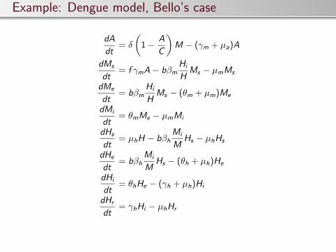
Example: Dengue model, Bello’s case

dA

dt= δ

(1− A

C

)M − (γm + µa)A

dMs

dt= f γmA− bβm

Hi

HMs − µmMs

dMe

dt= bβm

Hi

HMs − (θm + µm)Me

dMi

dt= θmMe − µmMi

dHs

dt= µhH − bβh

Mi

MHs − µhHs

dHe

dt= bβh

Mi

MHs − (θh + µh)He

dHi

dt= θhHe − (γh + µh)Hi

dHr

dt= γhHi − µhHr

Example: Dengue model, Bello’s case

R0 =b2βmβhθhθm

(θm + µm)(γh + µh)(θh + µh)µmM· f γmµm

δMC

(δM + C (γm + µa))

=b2βmβhθhθm

(θm + µm)(γh + µh)(θh + µh)µm· M

∗s

M

The Basic Reproductive Number (R0) of the epidemic occurred inBello in 2010 was between 1.5 and 2.7.

Example: Dengue model, Bello’s case

R0 =b2βmβhθhθm

(θm + µm)(γh + µh)(θh + µh)µmM· f γmµm

δMC

(δM + C (γm + µa))

=b2βmβhθhθm

(θm + µm)(γh + µh)(θh + µh)µm· M

∗s

M

The Basic Reproductive Number (R0) of the epidemic occurred inBello in 2010 was between 1.5 and 2.7.

Epidemiological data

The parameters used in the model, their biological descriptions,and their ranges of values.

Param. Meaning V. / day V. / week

b Biting rate [0, 1] [0, 4]

δ Per capita oviposition rate [8, 24] [55, 165]

γm Transition rate from the aquatic phase to the adult phase [0.125, 0.2] [0.875, 1.4]

µa Mortality rate in the aquatic phase [0.001, 0.5] [0.007, 0.3]

µm Mortality rate in the adult phase [0.008, 0.03] [0.06, 0.20]

f Fraction of female mosquitoes hatched from all eggs [0.42, 0.55] [0.42, 0.55]

C Carrying capacity of the environment [6400, 95000] [6400, 95000]

µh Birth and death rate of the human population 0.00006 0.0004

βh Transmission probability from mosquito to human [0, 1] [0, 1]

βm Transmission probability from mosquito to human [0, 1] [0, 1]

θm Transition rate from exposed to infectious mosquitoes [0.08, 0.13] [0.58, 0.88]

θh Transition rate from exposed to infectious humans [0.1, 0.25] [0.7, 1.75]

γh Recovery rate [0.07, 0.25] [0.5, 1.75]

Initial conditions

The initial conditions used in the model, their descriptions, andtheir ranges of values.

Initial condition Meaning Range

A(0) Initial condition for the aquatic phase [5755, 17265]

Ms(0) Initial condition for susceptible mosquitoes [0, 1200000]

Me(0) Initial condition for exposed mosquitoes [0, 100]

Mi (0) Initial condition for infectious mosquitoes [0, 100]

Hs(0) Initial condition for susceptible humans [244402, 321734]

He(0) Initial condition for exposed humans [18, 72]

Hi (0) Initial condition for infectious humans [6, 24]

Hr (0) Initial condition for recovered humans [81405, 158809]

The model fitted to the real biological data

Param. Value

δ 65

γm 1.4

µa 0.1156

b 4

µm 0.12

θm 0.58

f 0.5

θh 0.7

C 10000

γh 1

βm 0.6

βh 0.15

µh 0.0004

A(0) 9000

Ms(0) 1199976

Me(0) 18

Mi (0) 6

Hs(0) 321710

He(0) 18

Hi (0) 6

Hr (0) 81501

Stability analysis

Figure: Henri Poincare (April 29, 1854 - July 17, 1912). Image taken

from https://goo.gl/0I0qLJ

Figure: Aleksandr Lyapunov (June 6, 1857 - November 3, 1918).

Image taken from https://goo.gl/dLNfwW

DefinitionA point x∗ is called anequilibrium point ofx = f(x), if f(x∗) = 0.

Stability analysis

Figure: Henri Poincare (April 29, 1854 - July 17, 1912). Image taken

from https://goo.gl/0I0qLJ

Figure: Aleksandr Lyapunov (June 6, 1857 - November 3, 1918).

Image taken from https://goo.gl/dLNfwW

DefinitionA point x∗ is called anequilibrium point ofx = f(x), if f(x∗) = 0.

Definitions: stable, unstable and asymptotically stable

1

x∗

ε

x0

δ

Figure: The black line shows the definition of stable point. The greenline shows the definition of unstable point. The red line represents adefinition of asymptotically stable point.

Definitions: stable, unstable and asymptotically stable

DefinitionThe equilibrium point x∗ is

stable if, for each ε > 0, there is a δ = δ(ε) > 0 such that,

||x0 − x∗|| < δ ⇒ ||ϕ(t, x0)− x∗|| < ε, ∀t ≥ 0

unstable, if not stable

asymptotically stable, if it is stable, and δ can be chosen suchthat

||x0 − x∗|| < δ ⇒ limt→∞

||ϕ(t, x0)− x∗|| = 0

Stability diagram

Stability Analysis

x = f(x)x∗ equilibrium point

Use the Jacobian Matrix Df(x∗)to classify x∗ in:

Non-hyperbolic point (NH)

Hyperbolic point (H)

Based on the eigenvalues λ of Df(x∗)

Indirect Method of Lyapunov(Linearization)

Hyper

bolic poi

nts

Direct Method of Lyapunov

NH and H points

Indirect method of Lyapunov

The following results were taken from (Hale and Kocak, 2012).

TheoremLet f be a C 1 function. If all eigenvalues of the Jacobian matrixDf(x∗) have negative real parts, then the equilibrium point x∗ ofx = f(x) is asymptotically stable.

TheoremLet f be a C 1 function. If at least one of the eigenvalues of theJacobian matrix Df(x∗) has positive real part, then the equilibriumpoint x∗ of x = f(x) is unstable.

Indirect method of Lyapunov

The following results were taken from (Hale and Kocak, 2012).

TheoremLet f be a C 1 function. If all eigenvalues of the Jacobian matrixDf(x∗) have negative real parts, then the equilibrium point x∗ ofx = f(x) is asymptotically stable.

TheoremLet f be a C 1 function. If at least one of the eigenvalues of theJacobian matrix Df(x∗) has positive real part, then the equilibriumpoint x∗ of x = f(x) is unstable.

Indirect method of Lyapunov

Theorem(Grobman (1959) - Hartman(1960)) If x∗ is a hyperbolicequilibrium point of nonlinear system x = f(x), then there is aneighborhood of x∗ in which f is topologically equivalent to thelinear vector field x = Df(x∗)x.

Direct method of Lyapunov

The following result was taken from (Khalil, 1996).

TheoremLet x∗ = 0 be an equilibrium point of x = f(x). Let V : D → R bea continuously differentiable function on a neighborhood D ofx∗ = 0, such that

V (0) = 0 and V (x) > 0 in D − {0}

V (x) ≤ 0 in D

then, x∗ = 0 is stable. Moreover, if

V (x) < 0 in D − {0}

then x∗ = 0 is asymptotically stable.

Exponentially stable

DefinitionThe equilibrium point x∗ = 0 of x = f(x) is said to beexponentially stable if

‖x(t)‖ ≤ k‖x(0)‖e−λt , ∀t ≥ 0

k ≥ 1, λ > 0, for all ‖x(0)‖ < c .

DefinitionWhen all eigenvalues λ’s of a matrix A satisfy Re(λ) < 0, A iscalled a Hurwitz matrix.

TheoremThe equilibrium point x∗ = 0 of x = f(x) is exponentially stable ifand only if the linearization of f(x) at the origin is a Hurwitzmatrix.

Exponentially stable

DefinitionThe equilibrium point x∗ = 0 of x = f(x) is said to beexponentially stable if

‖x(t)‖ ≤ k‖x(0)‖e−λt , ∀t ≥ 0

k ≥ 1, λ > 0, for all ‖x(0)‖ < c .

DefinitionWhen all eigenvalues λ’s of a matrix A satisfy Re(λ) < 0, A iscalled a Hurwitz matrix.

TheoremThe equilibrium point x∗ = 0 of x = f(x) is exponentially stable ifand only if the linearization of f(x) at the origin is a Hurwitzmatrix.

Exponentially stable

DefinitionThe equilibrium point x∗ = 0 of x = f(x) is said to beexponentially stable if

‖x(t)‖ ≤ k‖x(0)‖e−λt , ∀t ≥ 0

k ≥ 1, λ > 0, for all ‖x(0)‖ < c .

DefinitionWhen all eigenvalues λ’s of a matrix A satisfy Re(λ) < 0, A iscalled a Hurwitz matrix.

TheoremThe equilibrium point x∗ = 0 of x = f(x) is exponentially stable ifand only if the linearization of f(x) at the origin is a Hurwitzmatrix.

How to find a Lyapunov function?

Polynomial System

Lyapunov’s polynomial

x = f(x)

function exists in abounded region

Exponentially stablenonlinear system

is

then

Open ResearchProblem

else

For a deeper discussion of when a Lyapunov’s polynomial functionexists in a bounded region we refer the reader to (Peet, 2009).

Counterexample

The system (1) does not admit a polynomial Lyapunov function ofany degree.

x = −x + xy

y = −y(1)

See (Ahmadi et al., 2011) for details of this result.

How to find a Lyapunov function?

Definition of Lyapunov function

V (x) ≥ 0

V =n∑

i=1

∂V

∂xixi = 〈∂V

∂xi, xi 〉

V ≤ 0

Relaxation of constraints

V (x) is a Sum of Squares (SOS)

−V (x) is a Sum of Squares (SOS)

Can we apply this results to epidemiological models?

Epidemiological Models

• Disease free point

• Endemic equilibrium point

R0 depends on theparameters and the initialconditions of the model

SIR Model

dS

dt= −βSI

dI

dt= βSI − γI

dR

dt= γI

Can we apply this results to epidemiological models?

Epidemiological Models

• Disease free point

• Endemic equilibrium point

R0 depends on theparameters and the initialconditions of the model

SIR Model

dS

dt= −βSI

dI

dt= βSI − γI

dR

dt= γI

Can we apply this results to epidemiological models?

dA

dt= δ

(1− A

C

)M − (γm + µa)A

dMs

dt= f γmA− bβm

Hi

HMs − µmMs

dMe

dt= bβm

Hi

HMs − (θm + µm)Me

dMi

dt= θmMe − µmMi

dHs

dt= µhH − bβh

Mi

MHs − µhHs

dHe

dt= bβh

Mi

MHs − (θh + µh)He

dHi

dt= θhHe − (γh + µh)Hi

dHr

dt= γhHi − µhHr

Bibliography

Khalil, H. K. (1996). Nonlinear systems. Prentice Hall.

Hale, J. K., Kocak, H. (2012). Dynamics and Bifurcations.Springer Verlag.

Peet, M. M. (2009). Exponentially Stable Nonlinear Systems havePolynomial Lyapunov Functions on Bounded Regions. IEEETransactions on Automatic Control, 54(5), pp. 979-987.

Ahmadi, A. A., Krstic, M., Parrilo, P. A. (2011). A globallyasymptotically stable polynomial vector field with no polynomialLyapunov function. In Proceedings of the 50th IEEE Conferenceon Decision and Control.