stability analysis of an earth embankment subjected...

UNIVERSITÀ DEGLI STUDI DI PADOVA

Dipartimento di Ingegneria Civile, Edile e Ambientale – ICEA

TESI DI LAUREA MAGISTRALE IN

INGEGNERIA PER L’AMBIENTE E IL TERRITORIO

STABILITY ANALYSIS OF AN EARTH EMBANKMENT SUBJECTED TO RAINFALL

INFILTRATION

(ANALISI DI STABILITÀ DI UN RILEVATO IN TERRA SOGGETTO AD INFILTRAZIONE DI

ACQUE DI PIOGGIA)

Relatore: Ing. Fabio Gabrieli Laureando: Daniele Bertoldo

Anno Accademico 2012/2013

Table of Contents

Chapter 1

Introduction ................................................................................................................................ 1

1.1. General ..................................................................................................................... 1

1.2. Objective and scopes ............................................................................................... 2

1.3. Outline of the thesis .................................................................................................. 3

1.4. Background .............................................................................................................. 4

Chapter 2

Theory for Infiltration Analysis .................................................................................................... 6

2.1. Introduction ............................................................................................................... 6

2.2. Conceptual infiltration models ................................................................................... 6

2.3. Analytical and numerical solutions ............................................................................ 9

2.3.1. Hydraulic Characteristics ..................................................................................... 11

2.3.1.1. Volumetric Water Content – Soil Water Characteristic Curve (SWCC) .............. 12

2.3.1.2. Hydraulic Permeability ...................................................................................... 13

Chapter 3

Theory for Saturated-Unsaturated Soil Consolidation ............................................................... 15

3.1. Introduction ............................................................................................................. 15

3.2. General ................................................................................................................... 15

3.3. Formulation of the Theory of Consolidation for an Unsaturated Soil ....................... 15

3.3.1. Stress State Variables ......................................................................................... 15

3.3.2. Constitutive Relationships ................................................................................... 16

3.3.2.1. Soil structure constitutive relationship ............................................................... 16

3.3.2.2. Water phase constitutive relationship ................................................................ 18

3.3.2.3. Relationships between the coefficients of volume change and elasticity parameters .................................................................................................................... 20

3.3.3. Flow Laws ........................................................................................................... 21

3.3.3.1. Flow of water..................................................................................................... 21

3.3.3.2. Flow of air ......................................................................................................... 22

3.3.4. Basic Equation of Physics ................................................................................... 23

3.3.4.1. Equilibrium equations ........................................................................................ 23

3.3.4.2. Water continuity equation .................................................................................. 23

3.3.5. Summary of the Formulation Theory for the Consolidation or Swelling Process in an Unsaturated Soil ........................................................................................................... 24

3.4. Numerical implementation of the volume–mass versus stress constitutive relations 25

3.4.1. Soil structure constitutive relation ........................................................................ 25

3.4.2. Water phase constitutive relation ......................................................................... 26

3.4.3. Computed material parameters ............................................................................ 27

3.4.4. Uncoupled and coupled solutions of soils behavior subjected to water flow ......... 28

3.4.4.1. Coupled Solutions ............................................................................................. 29

3.4.4.2. Uncoupled Solutions .......................................................................................... 29

Chapter 4

Theory of Slope Stability ........................................................................................................... 31

4.1. Introduction ............................................................................................................. 31

4.2. Basic concepts applied to slope stability .................................................................. 31

4.2.1. Saturated soil stresses ......................................................................................... 31

4.2.2. Saturated shear strength ..................................................................................... 31

4.2.3. Unsaturated soil stresses ..................................................................................... 32

4.2.4. Shear strength for unsaturated soils .................................................................... 34

4.2.5. Shear strength on “p’-q” diagram ......................................................................... 36

4.3. Slope stability considerations for embankment design ............................................ 38

4.4. Slope Stability Analyses .......................................................................................... 39

4.4.1. Infinite slope stability analysis method ................................................................. 39

4.4.1.1. Infinite slopes in dry cohesionless soils ............................................................. 40

4.4.1.2. Infinite slope in pure cohesive soil ..................................................................... 41

4.4.1.3. Infinite slope in cohesive frictional soil ............................................................... 41

4.4.1.4. Infinite slopes in cohesive frictional soils with parallel seepage .......................... 43

4.4.2. Finite slope stability analysis method ................................................................... 44

4.4.2.1. The Ordinary Method of Slices .......................................................................... 44

4.4.2.2. Other Methods ................................................................................................... 46

4.4.2.3. Considerations about the Methods of Slices ...................................................... 48

4.4.2.4. Finite Element Stress-Based Method ................................................................. 48

4.4.2.5. Influence of Soil Stratigraphy and Pore-Water Pressure .................................... 50

4.5. Undrained Instability and Static Liquefaction ........................................................... 51

Chapter 5

Rainfall Infiltration Analysis ....................................................................................................... 55

5.1. Introduction ............................................................................................................. 55

5.2. Relevant Theory ...................................................................................................... 55

5.3. Numerical Study of Slope Infiltration ........................................................................ 56

5.3.1. Results ................................................................................................................ 59

5.3.1.1. Steady-State Conditions .................................................................................... 59

5.3.1.2. Transient Conditions .......................................................................................... 60

5.3.2. Conclusions ........................................................................................................ 65

Chapter 6

Embankment Infiltration-Stress-Deformation Analysis .............................................................. 67

6.1. Introduction ............................................................................................................. 67

6.2. Numerical study ...................................................................................................... 70

6.2.1. Results ................................................................................................................ 72

6.2.2. Conclusions ........................................................................................................ 84

Chapter 7

Slope Stability Analysis ............................................................................................................ 86

7.1. Introduction ............................................................................................................. 86

7.2. Results ................................................................................................................... 88

7.2.1. Homogenous Soil Case ....................................................................................... 88

7.2.2. Non-homogenous Soil Case................................................................................ 98

7.3. Conclusions .......................................................................................................... 105

Chapter 8

Parametric Study .................................................................................................................... 107

8.1. Introduction ........................................................................................................... 107

8.2. Results and Discussion......................................................................................... 109

8.2.1. Slope Angle and Rainfall Intensity ..................................................................... 109

8.2.2. Threshold Rainfall Intensity ............................................................................... 111

8.2.3. Antecedent Rainfall ........................................................................................... 113

Chapter 9

Conclusions ............................................................................................................................ 119

References ............................................................................................................................. 122

1

Chapter 1

Introduction

1.1. General

Over the last several decades the world population has growth in both developing as well as the developed countries. As a result, to meet the continuously increasing demands of the public needs for transportation facilities and flooding defense, there has been a steady rise in the construction of new facilities such as roadways, railways, earth dam and levees. Some of these facilities are not only necessary to prevent traffic congestion or hydraulic protection of the landscape, but also to alleviate economic losses associated with the lack of them. However their failure may lead to loss of human life beside heavy economical losses. In many situations these facilities have to be built on or with compacted embankments. These last usually are classified as poor structures, in the sense that their cost must be reduced as much as possible, due to their huge extension. Traditional technologies – poor technologies – are still being used, relying on local experience and rules of thumb, which are still considered to be sufficient to guarantee sufficient margin of safety against failure and adequate working performance during embankment lifetime. However, since huge amounts of soil are required to build embankments for transportation facilities and flooding defense, and since the choice for optimal characteristics of the material is definitely limited by the requirement of the locally available soil, then the development of supplementary numerical tools and knowledge, able to analyze the behavior of these structures, may:

− help in the design − help in the interpretation of in situ control measurement − be advantageous to infer the suitability of the soils available in situ, especially in

developing countries where the need to bring huge amounts of soil from far borrow areas can be unfeasible.

The focus of embankment design is conventionally based on understanding the displacements of foundation ground rather than embankment itself. In addition, the variation of pore-water pressure with time during the construction of embankments is taken into account in the design when the foundation material at the construction site is cohesive in nature. As concern the stability of the slopes of the fill embankments the failures may happen due to human-induced factors, such as the artificial loading of the slope or the cutting away of the toe, improper soil compaction, groundwater pressure, slope toe erosion (due to the erosive action of the water river, as example). However in several situations, the instability of embankments is simply due to rainfall. The embankment stability analyses are usually performed using conventional limit equilibrium method assuming the embankment is in a state of saturated condition. This assumption is believed to provide a conservative design approach in the assessment of the stability of slopes constructed with compacted soils. However, this approach for the design of embankments may not always be satisfactory since these structures typically remain unsaturated throughout most of their working life. Therefore it should be more appropriate to design them using the mechanics of unsaturated soils, even if it is seldom considered, also in developed countries. It is worth noting that usually the stress levels of interest in this kind of geotechnical structures are rather low, due to normally limited height of the embankments and absence of relevant surcharge loading. On the contrary these are exposed to significant environmental loads, as the

2

aforementioned rainfalls, which induce an increasing number of wetting-drying cycles over time and a continuously variable water content in the soil, especially in the most shallow layers interacting with the atmosphere. Instability of unsaturated soil slopes during wet periods has been observed in many countries, for both natural and man-made slopes, and there is evidence to demonstrate that infiltration of rainfall into unsaturated slopes forms a wetted zone, which more likely triggers shallow slip failures (Cho SE, Lee SR. (2002)). This is true for both the granular soils and cohesive finer soils. These last, particularly, show shrinking/swelling cycles, according to the drying/wetting cycles, which open fissures and reduce the density; actually the soil is weakened and cannot resist anymore resulting in slip-plane failures. Rainfall infiltration commonly causes the loss of the strength contribution due to matric suction and the subsequent increase in positive pore-water pressures. The strength contribution due to matric suction is an important feature of the unsaturated soils which allow the slopes to be safe even at much steep angles when unsaturated conditions are maintained, but to fail when the suction is lost due to water infiltration. All the above considerations suggest that stability analysis of embankments should be carried out also considering infiltration conditions beside the conventional most critical stages. The usual conventional most critical stages arise always from an excess of the pore water pressure but they don’t provide for the rainfall situation. These critical stages are:

− at the end of construction: in this case the pore water pressure excess depends by the applied overburden pressures.

− during steady state seepage, in case of embankment dams: here the pore water pressure excess results from natural groundwater condition.

− during rapid drawdown of the level in the reservoir, always in the case of embankment dams: here the pore water pressure excess results from natural groundwater condition.

Therefore, an overall reasonable embankment stability analysis should include also the influence of rainfall infiltration. This can be assured only when the distribution of matric suction within the embankments are taken into account together with the unsaturated soil mechanics. However the following considerations have to be taken in mind:

a) the measurement of pore-water pressures in embankments is expensive, time consuming (as it is ruled by seasonal variation of climate), and generally not feasible along the whole embankment.

b) laboratory investigations on unsaturated soil samples retrieved from the compacted structure on-site are not allowed usually, as the authorities, who manage the structure, discourage sampling after construction to preserve structural integrity; and the representativeness of samples compacted in the laboratory against of the soil compacted in situ has not yet been verified in detail.

In this framework the development of numerical tools able to reproduce the soils behavior in saturated-unsaturated conditions can be perceived as a great opportunity. The results from the numerical analyses can revert into new knowledge of the real phenomena observed on field, and also into new preliminary specifications that can be suggested for new constructions.

1.2. Objective and scopes

In the present thesis, an attempt was made to study how the rainfall infiltration influences the stresses and the behavior of a soil embankment according to different hydraulic permeability

3

values and rainfall intensities. In particular the analyses performed can be distinguished in four main types:

• an infiltration analysis: to study how infiltration into an embankment varied with respect to rainfall intensity and respect to the lateral and/or top sides of the bank, considering both steady and transient conditions.

• an infiltration-stress-deformation analysis: to study, using the incremental strain-stress relationship for saturated/unsaturated soils, the stresses and deformations induced by rainfall infiltration into the embankment.

• a slope stability analysis: two different approaches to develop the limit equilibrium method are tested to evaluate that which better catches the effect of rainfall infiltration on slopes embankment. It was also investigated the case of non-homogeneous embankment having slope-parallel layers with different strengths and permeability in order to find the right specifications to follow in this kind of analyses when rainfall infiltration is considered.

• a parametric study: to study how the rainfall intensity, the hydraulic permeability, the initial degree of saturation in the soil and the geometry affect the variation of the factor of safety (FS) of the slope embankment.

Finite element analyses were undertaken using the Geo-Slope software (SEEP/W, SIGMA/W and SLOPE/W) considering infiltration of water due to different rainfall events as the unique load on the embankment. One of the most powerful features of GeoStudio is the smooth integration that exists between all the individual programs. Several conclusions of engineering practice interest are derived in the present thesis.

1.3. Outline of the thesis

This thesis is organized into nine chapters. Chapter 1, "Introduction", presents a general preamble to introduce the topic and the need for this research study, the objectives and scope of the research study, the outline of the thesis and a background about the arguments dealt. Chapter 2, “Theory for Infiltration Analysis”, presents the different models developed to describe the infiltration and the seepage of water into the soil. Conceptual models, analytical and numerical solutions are introduced. Hydraulic characteristics necessary to solve the equation governing the water flow are also presented and explained. Chapter 3, “Theory for Saturated-Unsaturated Soil Consolidation”, presents the physical relationships required to describe the three-dimensional behavior of partially saturated soils, and the development of coupled equations for the simulation of the volume change problems. The finite element formulation of the coupled equations is derived for a plane strain problem with the assumption that a continuous air phase is maintained at atmospheric pressure. Peculiarities related to coupled and uncoupled analysis are presented. Chapter 4, “Theory of Slope Stability”, presents the soil stresses and the shear strength formulations for both the saturated and unsaturated soils, the slope stability analysis methods for both infinite and finite slopes, and a last section dealing with the undrained instability and the static liquefaction phenomena. Chapter 5, “Rainfall Infiltration Analysis”, presents a numerical study on the process of rainfall infiltration into a designed embankment. Various rainfall intensities are considered and the

4

infiltration fluxes are calculated along the three different sides of the bank for both steady-state and transient condition. Chapter 6, “Embankment Infiltration-Stress-Deformation Analysis”, presents the stress paths and the time evolution of suction and deviatoric stress obtained, with a numerical study, for two different hydraulic conductivity soil types subjected to a steady rainfall. Results and considerations are discussed. Chapter 7, “Slope Stability Analysis”, presents the numerical results of slope stability analyses on the same embankment subjected to a steady rainfall considered in the Chapter 5 and 6. It includes two main parts. The first part contains the results obtained considering two homogeneous soil embankments with different hydraulic conductivity. The second part consider a non-homogeneous soil embankment and investigates which specifications should be followed in such stability analysis to catch properly the effect of rainfall. Chapter 8, “Parametric Study”, presents the results of three parametric studies performed, always with a numerical software, to asses which factors have more influence on the slope stability (safety factor). The factors investigated are: rainfall intensity, hydraulic permeability, initial degree of saturation and slope angle. Chapter 9, “Conclusions”, reports the main conclusions of the thesis work.

1.4. Background

The movement of water into soil due to rainfall or irrigation activity is known as infiltration. The infiltration of water into soil is governed by the relationship between the rate of water application (or rainfall intensity) and the soil infiltration capacity. If the rate of water application exceeds the soil infiltration capacity, ponding or runoff occurs over the soil surface. It has been found that infiltration rate is relatively high in the early stages of an event and, then, it decreases with time to reach a steady value if the rain lasts for a sufficient long time. This steady value was predicted to be equal to the saturated coefficient of permeability (��) by many authors, however it has been observed through on field experiments that actually it is a percentage of �� and it is variable according to the soil type and the ground surface geometry (Li et al., 2005; Rahardjo et al., 2005). Studies by several investigators demonstrate that shallow slip failures parallel to the slope surface are possible due to rainfall infiltration (Blatz et al. (2004), Rahardjo et al. (2001)). Rainfall-induced slope failures commonly occur in the unsaturated zone above groundwater table in many steep residual soil slopes. During a rainy season, desiccated soils with higher permeabilities will increase rain infiltration into slopes causing an increase in pore-water pressures in the zone above the groundwater table. In addition, the groundwater table may rise to result in a further increase in pore-water pressures. As a result, the shear strength of the soil will decrease and factor of safety of the slope can decrease to below a critical value, triggering slope failure. In case of natural slopes, this characteristic failure behavior allows analyzing instability of saturated-unsaturated soil slopes assuming them as infinite slopes. The method used in traditional infinite slope analysis must be modified to take into account the variation of the pore water pressure profile that results from the infiltration process (Duncan and Wright, (1995)). For an infinite slope with seepage parallel to the slope surface, the safety factor for the slip surface at depth H is:

�� sin � cos � � tan �tan � � �� tan �� tan �

5

where FS is the safety factor, � is the effective cohesion, � is the effective friction angle, � is the slope angle, �� is the saturated unit weight of the soil and � is the ratio between the distance from the groundwater table to the slip surface and H. Here the slip surface is assumed to be below the groundwater table in the saturated zone. However, sometimes it was observed that soil suction has not to be reduced to zero to trigger a failure; in this case, based on the extended Mohr–Coulomb failure criterion (Fredlund et al., 1978), the safety factor of an unsaturated uniform soil slope can be expressed as:

�� tan �� tan �′�� sin � cos �

where � is the total unit weight of the soil, �� is the pore air pressure, �� is the pore water pressure, �� is the matric suction, �� is the total normal stress, �� is the net normal stress on the slip surface and �� is an angle indicating the rate of increase in shear strength related to matric suction. In case of artificial compacted embankments the above described concept is not always justified because the finite height may prevent the development of an actual infinite slope failure mode. Moreover, it is not always easy to determine earlier if a rainfall produced saturated or unsaturated conditions in the surficial layer. Therefore, besides the infinite slope-stability analysis method, other methods are employed to calculate the safety factor. These are the two-dimensional methods of slices for slope stability. The inputs required are the geometry and soil profiles of the slope, the shear strength parameters (the extended Mohr–Coulomb failure criterion is usually adopted), the soil densities, and the pore water pressure distribution throughout the slope. The pore water pressure distributions used as input data in the limit equilibrium slope stability analysis can be classified into three types:

i. calculated pore water pressure distribution from numerical seepage analyses, ii. assumed pore water pressure distribution based on the wetting front concept, and iii. actual field-measured pore water pressures.

Therefore the water flow behavior associated with rainfall infiltration is required to assess the embankment stability. This is possible using the coefficient of permeability function for unsaturated soils as an input parameter in the slope stability analysis. The coefficient of permeability function is the relationship which describes the variation of coefficient of permeability with respect to matric suction values. This relationship can be predicted using the Soil–Water Characteristic Curve (SWCC) and the coefficient of permeability under saturated condition (��).

6

Chapter 2

Theory for Infiltration Analysis

2.1. Introduction

Infiltration plays a significant role in the instability of slopes under rainfall conditions. The effect of seepage on natural slope stability is typically addressed in most analyses by calculating the factor of safety or critical depth for an infinite slope subject to seepage parallel to the slope surface. This type of analysis assumes that saturated steady-state flow is taking place over a given depth (see section 4.4.1.4 in Chapter 4). In order to simplify the analysis as a worst-infiltration scenario, it is often assumed that the phreatic surface (groundwater level) rises up to coincide with the slope surface, and that the slope is completely saturated. For such saturated slopes, additional infiltration is not possible, and additional simulated rainfall will have no further effect on slope stability. However, in many situations where shallow failures are concerned, it has been noted that there is not much evidence of a rise in the water table sufficient to trigger the observed failures. Instead, the failures have been attributed to the advancement of the wetting front into slopes until it reaches a depth where it triggers the failure. In these cases, for slopes that are initially unsaturated, the rainfall will yield a different effect. Firstly the pore water pressure pattern, that develops in the soil, will occur as a transient process as the infiltrating water moves downwards into the soil. Secondly, the shear strength of the soil will depend on soil suction, and hence on the pore water pressure profile, and will vary in time. In order to describe the advancement of wetting front and the flow of water into the porous soil medium, both conceptual infiltration models and solutions of the Richards (1931) equation (analytical and numerical) have been proposed.

2.2. Conceptual infiltration models

Infiltration models based on a wetting front concept have been proposed as response to the limitations of complex numerical solutions to solve the Richards (1931) equation, which rigorously computes infiltration and soil moisture profiles in saturated–unsaturated soil systems. Among the many conceptual infiltration models it must be remembered the followings: Green and Ampt, (1911); Lumb, (1962); Mein and Larson, (1973); Sun et al., (1998). All them have been proposed with the intent to bypass:

− the natural spatial variability occurring in the field, − the uncertain initial and boundary conditions, and − the complexity of the numerical solution for practical applications.

The amount of rainfall that can infiltrate the ground at a given time ranges from zero to the infiltration capacity, which is a function of the initial moisture content and rainfall intensity. Infiltration capacity is the maximum rate at which a given soil can absorb water; it varies with time and decreases approaching a minimum value (approximately equal to the saturated hydraulic conductivity) as infiltration continues.

Green and Ampt, (1911) first derived the first physically based equation describing the infiltration capacity of a soil. The Green–Ampt infiltration model was initially proposed to describe infiltration through partially saturated soil underlying ponded water (fig. 1). It is based

7

on Darcy’s law. Above the wetting front, the soil is assumed to be completely saturated, while the soil below the wetting front remains at the initial water content. It is assumed that the coefficient of permeability in the wetted zone, ��, does not change with time, and that there is a constant suction head !" at the wetting front.

Fig. 1: Illustration of Green–Ampt infiltration mod el

At any time T, the infiltration capacity # , by applying Darcy’s law, can be stated as follows:

#$�%� � �� &'&x � �� &�) � !"�&x

where: �� = coefficient of permeability in the wetted zone ' = total hydraulic head ) = elevation above a reference plane !" = matric suction head x = arbitrary direction

Hence in the z direction, the infiltration capacity at the wetting front is given as:

#*�%� � �� +1 � !"-" . � �� +-" � !"-" . � /F/%

where: !" = constant suction head at the wetting front -" = depth of the wetting front.

The value of hydraulic conductivity above the wetting front, ��, depends on the soil type and on the degree of saturation, and it can be measured in the field. The suction head at the wetting front !" is a function of soil water content, and can be determined from experimental

measurements.

8

Integration on time of the above equation for the infiltration capacity yields the following expression for the cumulative infiltration F:

F � -� ∆23 � ��% � ∆23!" ln 5!" � -�!" 6

where: ∆23 = the moisture deficit, expressed as the difference between the volumetric water contents before and after wetting.

Therefore, the time necessary to saturate the soil to the depth -� can be written as:

%� � ∆23�� +-� � !" ln 5!" � -�!" 6. To consider the conditions in which rainfall intensity is initially less than the infiltration capacity of the soil, Mein and Larson (1973) modified the Green–Ampt model, and developed a simple two-stage model for predicting infiltration before and after surface ponding. Lumb (1962) introduced the wetting front concept in relation to the investigation of slope failures in Hong Kong. Under prolonged and heavy rainfall, the depth, -", of the wetting front is defined

as:

-" � �� 789�" � �:;

where �� is the saturated coefficient of permeability, �" is the final degree of saturation, �: is

the initial degree of saturation, 8 is the porosity of the soil and t is time. Lumb’s wetting front equation implies that ground surface flux (<) is equal to ��. In the case when rainfall is less intense than ��, the advance of the wetting front will be slower than that given by the above equation. Sun et al. (1998) proposed a generalized wetting band equation based on Lumb’s (1962) equation. In fig. 2 is shown a typical variation of soil suction with depth in an unsaturated soil. For a given ground surface flux <:, less than ��, under steady-state conditions, the pore water pressure is u:. If the ground surface flux is increased to <>, a new infiltration zone with pore water pressure u> will be formed that gradually progresses downwards with time. The depth of the wetting front can be calculated using the equation:

-" � �<> � <:�7�?> � ?:�

where ?: is the initial volumetric water content, which corresponds to u:; and ?> is the final volumetric water content, which corresponds to u>. The comparison between the predicted advance of the wetting front obtained from this equation and that from numerical seepage analysis of saturated - unsaturated soils, indicates reasonably accuracy of the formula for intense rainfall events which produce transition zones (wetting fronts) relatively sharp.

9

Fig. 2: Transient infiltration in an unsaturated soil (from Sun et al., 1998)

2.3. Analytical and numerical solutions

Serious limitations impose restrictions on the use of the conceptual infiltration models, because they usually do not consider:

a) sloping ground conditions, b) down-slope flows, c) non-homogeneous spatial distribution of initial moisture content d) variation of rainfall intensity, and e) the dependence of soil permeability on moisture content.

In addition, there will not always be a distinct difference between the infiltration zone and the zone in which the negative pore water pressures have been maintained, as it is actually considered by the conceptual models. To obtain a more rigorous distribution of pore water pressure in a slope under complex boundary conditions, the equation for the flow of water through an unsaturated–saturated soil system must be solved. This equation is based on the Darcy’s law and the mass conservation for water phase into soil, and it was derived by Richards (1931). Analysis of Richards’ equation yields approximations that describe the development of near-surface groundwater pressures in response to rainfall over varying periods of time. The unsteady and variably saturated Darcian flow of groundwater in response to rainfall infiltration in a sloping surface can be described by the Richards’ equation with a local rectangular Cartesian coordinate system (fig. 3) as follow:

&!&7 /?�/! � &&@ A�B�!� C&!&@ � sin DEF � &&) A�B�!� C&!&)EF � &&- A�*�!� C&!&- � cos DEF where:

10

! = is the ground water pressure (it is used the common symbol of suction, instead of the usual '�, because the water pressure in the infiltration analyses is usually negative, meaning suction is present into soil) ?� = the volumetric water content D = the slope angle 7 = time �B�!� = hydraulic conductivities in lateral direction (x and y), function of soil properties

and groundwater pressure head �*�!� = hydraulic conductivities in slope-normal direction (z), function of soil properties and groundwater pressure head

The coordinate x points down the ground surface; y points tangent to the topographic contour that passes through the origin; z points into the slope, normal to the x–y plane.

Fig. 3: Definition of the local, rectangular, Carte sian coordinate system used to analyze Richards equ ation. The origin lies on the ground surface, x is tangent to the local surface slope, y is tangent to the lo cal topographic contour, and z is normal to the x-y pla ne. The slope angle a is measured with respect to

horizontal (from Iverson, R. M. (2000)).

The solution of the above second-order partial differential equation is complicated, because the soil-water characteristic curve (the relationship ! � ?�) and the unsaturated permeability function (the relationship ! � �B,*) are strongly non-linear. Analytical solutions, if available, have the advantages of explicitness and simplicity over numerical simulations. Several analytical and quasi-analytical solutions to unsaturated flow problems have been developed. As example Iverson (2000) developed a mathematical model that uses a reduced form of Richards’s equation in vertical direction to evaluate effects of rainfall infiltration on landslide occurrence, timing and depth, in diverse situations. The model was considered for the case of shallow soil and rainfall time shorter than the time necessary for the transmission of lateral water pressure. The soils was assumed initially wet (� H ��). It was assumed the rainfall can infiltrate totally into the soil if the rainfall intensity is less than or equal to the saturated permeability. When the rainfall intensity is greater than the saturated permeability, then the infiltration rate is equal to the saturated permeability and the surplus rainfall runs off the slope as surface flow. This assumption is also adopted in some conceptual models for infiltration

11

capacity prediction, such as the Green–Ampt model. However such assumption may not be reasonable as field measurements (Li et al., 2005; Rahardjo et al., 2005) have shown that this is not the case. The on-field studies made by Li et al. (2005) showed that runoff may begin before the near-surface soils became fully saturated. Rahardjo et al. (2005) applied an artificial rainfall, 13x10-6 m/s in intensity, to an initially unsaturated soil slope with �� of 5,18x10-6 m/s and found that the infiltration capacity of the slope converged, after long time, to 2x10-6 m/s (≈ 0,4 ��). Also the results obtained with a numerical study in this thesis (see chapter 5 ’Rainfall Infiltration Analysis’) showed that the initial infiltration rate can be larger than �� but after it gradually decreased to a steady-state value that is less than ��. Therefore, if Iverson’s solution is used, unrealistically high pressure heads can be obtained due to the overestimation of infiltration rate. Furthermore the Iverson’s hydrological modelling of hillslope is generally valid, together with the infinite slope stability analysis, for the case of shallow landslides with a small depth compared to its length. In case of earth embankment, with a finite height, often the failure way may not be like infinite slope type, and the previous hydrological model cannot be applied anymore. Moreover the rise of the water table from the base of the embankment produces water soil distributions which are not comparable with the Iverson’s analytical solution hypotheses. Hence analytical solutions for the infiltration problem can be obtained only by making some assumptions which often does not reflect what is the actual conditions, and they can work well only under some specific initial and boundary conditions. In this framework the usage of numerical solutions can take great advantages and practical simplifications. Many computer programs have been developed for numerical modelling of seepage and infiltration in both saturated and unsaturated soils. In this thesis the potentialities of the SEEP/W finite element program has been exploited. Numerical solutions of Richard’s equation allow to consider whatever geometric soil configuration and whatever type of initial and boundary conditions (means initial moisture distributions and applied rainfall intensities). Furthermore, it is not considered a marked difference between the infiltration zone and the zone where the negative pore water pressures are maintained, because the wetting front concept is not applied in the numerical solutions, and so more realistic pore-water pressure profiles can be deduced. So, the helps coming from the finite element software seems to be unavoidable to study the soil embankment behavior under rainfall infiltration.

2.3.1. Hydraulic Characteristics

The water flow through unsaturated–saturated soils is strongly influenced by the unsaturated zone; the computer model SEEP/W, used in this thesis, performs analysis of both transient and steady-state water flow through unsaturated–saturated soils, and it simulates moisture flux throughout the entire flow domain. The derivation of the equation governing the water flow through unsaturated–saturated soils is attributed to Richards (1931). The governing equation arises from a consideration of mass conservation in an unsaturated–saturated medium in conjunction with an equation of motion, the Darcy’s law. For a two-dimensional domain it is as follow:

&&@ C�I�?�� &'�&@ E � &&) C�J�?�� &'�&) E � � &�?��&7

Darcy’s law has been shown to be valid for the water flow through unsaturated soils as well as for flow through saturated soils.

12

The main difference is that, unlike saturated soils, the permeability of an unsaturated soil is not constant but it depends on the pore volume occupied by water (the volumetric moisture content). So to implement Richards’ equation, the permeability have to be defined in relation to the volumetric water content ?�, which can be seen as the product of the porosity (8�and the degree of saturation (��: ?� � 8� . Therefore, in order to solve the above equation, two soil parameters must be determined: the volumetric water content ?�, and the permeability coefficients �I,J�?��.

2.3.1.1. Volumetric Water Content – Soil Water Characteristic Curve (SWCC)

In a saturated soil, all the voids are filled with water and the volumetric water content of the soil is equal to the porosity of the soil according to:

?� � 8�

where: 8 = porosity � = relative degree of saturation

In an unsaturated soil, the volume of water stored within the voids will vary depending on the matric suction within the pore-water, where the matric suction is defined as the differences between the air (��) and water pressure (��) as follows: (�� ). There is no fixed water content in time and space and so a function is required to describe how the water contents change with different pressures (suction values) in the soil. The volumetric water content function describes the capability of the soil to store water under changes in matric pressures. A such typical function is shown in fig. 4, and it is commonly called as soil water characteristic curve (SWCC).

Fig. 4: Volumetric Water Content function (or soil w ater characteristic curve - SWCC)

The three main features that characterize the volumetric water content function are the air-entry value, (AEV), the slope of the function for both the positive and negative pore-water pressure ranges (designated as Mw), and the residual water content, (?K).

13

The air-entry value (AEV) corresponds to the value of negative pore-water pressure when the largest voids begin to drain freely. It is a function of:

− the maximum pore size in the soil

− the pore-size distribution within the soil.

For higher pore size the air-entry value (AEV) moves to zero pressure values. A wider pore-size distribution implies the presence of some pores smaller than those of a uniform sand. Consequently, a more negative pore-water pressure must be applied before drainage begins because the SWCC is shifted to the left (the AEV assumes a more negative value). The slope of the function, Mw, is equivalent to the coefficient of compressibility for one-dimensional consolidation, Mv, in the positive pore-water pressure region. While in the negative pore-water pressure range, Mw varies over a range of values from the AEV to the pressure at the residual water content, and it represents the rate at which the soil stores or loses water as the pressure changes within the pore-water. Another key feature of the volumetric water content function is the residual volumetric water content, which represents the volumetric water content of a soil where a further increase in negative pore-water pressure does not produce significant changes in water content.

It is not especially difficult to obtain a direct measurement of a volumetric water content function in a laboratory (using the apparatus known as ‘Richard’s pressure plate cell’), but it does require time and it requires finding a geotechnical laboratory that performs the service. Then it may be advantageous, in terms of time and money, to get an estimation of the volumetric water content function using either a closed-form solution that requires only some curve-fitting parameters, or to use a predictive method that uses a measured grain-size distribution curve. The software SEEP/W has three methods available to develop a volumetric water content function. One estimate the function using a predictive method based on the grain-size distribution curve knowledge (‘Modified Kovacs’ estimation method). The other two are closed form equations based on known curve fit parameters:

− Fredlund and Xing (1994) method

− Van Genuchten (1980) method

In addition to these methods GeoStudio provide a list of 20 fully defined water content functions. In the following of the thesis all the analysis has been developed using, as volumetric water content function, one of the GeoStudio’s library which was calculated based on the Fredlund and Xing (1994) prediction method.

2.3.1.2. Hydraulic Permeability

The ability of a soil to conduct water is reflected by the hydraulic conductivity function. In a saturated soil, all the pore spaces between the solid particles are filled with water and the permeability is at its maximum value (saturated coefficient of permeability, ��). Once the air-entry value is exceeded, air enters the largest pores; air-filled pores become non-conductive to flow and they increase the tortuosity of the flow path; as a result, the ability of the soil to transport water (the hydraulic conductivity) decreases. As pore-water pressures become increasingly more negative, more pores become air-filled and the hydraulic conductivity decreases further. Therefore the hydraulic permeability for unsaturated soils are dependent on the volumetric water content, which is in turn related to the water pressure or matric suction. In other words, the ability of the unsaturated soil to transport water varies with soil suction.

14

The coefficient of permeability is related to the negative pore-water pressure in a nonlinear fashion. Actually measuring the hydraulic conductivity function is a time-consuming and expensive procedure, but the function can be readily developed using one of several predictive methods that utilize a measured or predicted volumetric water content function and the saturated hydraulic conductivity (��). The software SEEP/W has three separate methods built into the model that can be used to predict unsaturated hydraulic conductivity by volumetric water content function:

− Fredlund et al. (1994) method

− Green and Corey (1971) method

− Van Genuchten (1980) method

All these three estimation methods generally predict the shape of the function once it is specified the saturated hydraulic conductivity value (��), which is easily to obtain. In the following of the thesis, all the hydraulic conductivity functions, used to define the hydraulic properties of the soils, has been estimated using Fredlund et al. (1994) method.

15

Chapter 3

Theory for Saturated-Unsaturated Soil Consolidation

3.1. Introduction

There is a wide variety of practical problems where it is important to include both the unsaturated and the saturated consolidation in an analysis. A common situation is the placement of fill on the ground surface where the water table is at some depth. The transient conditions of the water table due to the applied load make it necessary to include both the saturated and the unsaturated consolidation. Another situation, where a form of consolidation in saturated-unsaturated conditions can be known, is that of the shrinking and swelling of soils occurring near the surface due to environmental changes. The soil changes volume in response to an applied loading arising from a change in negative pore-water pressure (or suction). The process is similar to consolidation. An unsaturated–saturated analysis is consequently required to correctly model such volume-change behavior.

3.2. General

Unsaturated soils can generally be divided into two groups with respect to volume change; namely, expansive soils and collapsible soils. Volume change is a result of a change in matric suction for both groups of soils. Expansive soils increase in volume when wetted while collapsible soils decrease in volume when wetted. The theory of unsaturated soil behavior is required for the study of either expansive soils or collapsible soils. In this chapter is presented a review of stress state variables, constitutive relationships, and flow laws for unsaturated soils. Soil properties required in the constitutive relationships are pointed out. Relationships between the coefficients of volume change and elasticity parameters are presented. The implementation of the constitutive equations into two finite element codes is illustrated.

3.3. Formulation of the Theory of Consolidation for an Unsaturated Soil

The behavior of unsaturated soils can be explained using the general theory of unsaturated soils, through the use of stress state variables, the constitutive relationships for soil structure and water phase, and the flow laws for the fluids.

3.3.1. Stress State Variables

The single stress state variable controlling the behavior of a saturated soil is the well accepted and experimentally verified Terzaghi’s effective stress (Terzaghi, 1936), denoted as �′, and expressed as:

� � � � ��

where: � = total normal stress, and

16

�� = pore-water pressure.

There have been several attempts to extend the effective stress equation for unsaturated soils. As example, Bishop (1959) defined the stress state in the form of an equation which include the pore-air pressure and a soil property:

� � �� L�� where: �� = pore-air pressure, and L = a parameter related to the degree of saturation of soils (called Bishop's parameter).

However several researchers pointed out some questions about this expression. Jennings and Burland (1962) suggested that Bishop's equation did not provide an adequate relationship between volume change and effective stress for most soils, particularly those below a critical degree of saturation. Moreover it was found that it can be used more accurately for shear strength behavior than for volume change (Bishop and Blight, 1963). Therefore the research was addressed to find more than one stress state variable to describe the behavior of unsaturated soils. Fredlund and Morgenstern (1977) proposed that the constitutive behavior of unsaturated soils be described using two independent stress state variables; namely, net normal stress, (� � ��), and matric suction, (�� ). The validity of these independent stress variables have now become well accepted and forms the basis for the formulations of shear strength and volume change problems for unsaturated soils (Fredlund and Rahardjo, 1993).

3.3.2. Constitutive Relationships

Volume change constitutive relationships relate the stress state variables to the deformation variables of a continuum through the use of elasticity parameters. In general, two constitutive relationships are presented to describe the volume change associated with an unsaturated soil; one relationship for the soil structure (in terms of volumetric strain) and another for the water phase (in terms of degree of saturation or water content).

3.3.2.1. Soil structure constitutive relationship

The soil structure constitutive relationship can be presented in various forms such as elasticity form and compressibility form. In elasticity form, the relations associated with the normal strains in the x-, y-, and z-directions are as follows (Fredlund and Morgenstern, 1976):

MI � ��I � ��N � ON 9�J � �* � 2��; � ��

MJ � 9�J � ��;N � ON ��I � �* � 2��

M* � ��* � ��N � ON 9�I � �J � 2��; � ��

17

where: N = elasticity parameter for the soil structure with respect to a change in the net normal stress, (� � ��), � = elasticity parameter for the soil structure with respect to a change in matric suction, (�� ) O = Poisson’s coefficient, and �I , �J, �* = total normal stress in the x-, y-, and z-directions.

The constitutive equations associated with the shear deformations are:

IJ � QRST ,J* � QSUT , *I � QURT

where: VIJ = shear stress on the x-plane in the y-direction (i.e., VIJ = VJI), VJ* = shear stress on the y-plane in the z-direction (i.e., VJ* = V*J), V*I = shear stress on the z-plane in the x-direction (i.e., V*I = VI*), and

G = shear modulus.

The constitutive equations can also be applied to situations where the stress versus strain relationships are non-linear applying an incremental procedure using small increments of stress and strain. Then, the non-linear stress versus strain curve is assumed to be linear within each stress and strain increment, while the elasticity parameters, E and H, may vary in magnitude from one increment to another. The soil structure constitutive relations associated with the normal strains can be written in an incremental form as follows:

/MI � /��I � ��N � ON /9�J � �* � 2��; � /��

/MJ � /9�J � ��;N � ON /��I � �* � 2�� /��

/M* � /��* � ��N � ON /9�I � �J � 2��; � /��

A change in the volumetric strain of the soil for each increment, /MW, can be obtained by summing the changes in normal strains in the x-, y-, and z-directions:

/MW � /MI � /MJ � /M*

where: /MW = change in volumetric strain for each stress increment.

Substituting the three equations of /MI , /MJ and /M* into that of /MW gives the volumetric strain

for a particular loading increment of the general three dimensional loading conditions:

18

/MW � 3 C1 � 2ON E /��YZ�� 3� /�� where: �YZ�� = mean total normal stress [9�I � �J � �*; 3⁄ ].

Fredlund and Rahardjo (1993) presented the constitutive relationship for soil structure in a compressibility form for the general, three-dimensional loading conditions:

/MW � �>�/��YZ�� \�/��

where:

�>� � 3 ]>^\_` a, coefficient of volume change with respect to a change in net normal

stress, �\� � bc , coefficient of volume change with respect to a change in matric suction.

The unloading constitutive relationship for soil structure is presented graphically in the form of constitutive surface in fig. 5.

Fig. 5: Constitutive surfaces for soil structure of an unsa turated soil.

3.3.2.2. Water phase constitutive relationship

The water phase constitutive relationship, in an elasticity form, based on a linear combination of the stress state variables, can be written as Fredlund and Rahardjo (1993):

/d�d: � 3N� /��YZ�� 1�� /�� where: N� = water volumetric parameter associated with a change in the net normal stress, and

19

�� = water volumetric parameter associated with a change in matric suction.

Using a compressibility form, the constitutive relationship for water phase can be written as follows:

/d�d: � �>�/��YZ�� \�/�� where: �>� � b̀e , coefficient of volume change with respect to a change in net normal stress,

and �\� � >ce , coefficient of volume change with respect to a change in matric suction.

The constitutive relationship for water phase is presented graphically in the form of constitutive surface in fig. 6.

Fig. 6: Constitutive surfaces for water phase of an unsaturated soil.

From equation for volumetric strain of soil structure in a compressibility form:

/MW � �>�/��YZ�� \�/��

the mean net normal stress can be expressed as a function of volumetric strain and matric suction, as follows:

/��YZ�� 1�>� /MW � �\��>� /�� where: >Yfg � `b�>^\_� , and

YhgYfg � ` c⁄�>^\_� .

20

Using this expression of mean net normal stress, the constitutive relationship for water phase, in compressibility form, can be written as:

/d�d: � ��>/MW � ��\/�� where:

��> � YfeYfg , or in the elasticity form, `�>^\_�`e

��\ � �\� � YfeYhgYfg , or in the elasticity form, >ce � b`�>^\_�`ec

This equation is similar in form to the constitutive equation for the water phase presented by

Dakshanamurthy et al. (1984):

?� � d�d: � �MW � C1i � 3�� E �� MW � j��

where: � � `�>^\_�c

j � 1 i⁄ � 3 � �⁄ i is the modulus relating a change in volumetric water content to a change in matric suction �� ; so it is the same of ��.

This equation separates the change in volumetric water content into two components. One component is due to the volumetric strain of the soil, and the other component is due to change in matric suction. At full saturation of the soil, the change in volumetric water content is equal to the change in volumetric strain. Mathematically, the fully saturated condition is satisfied by setting � = 1 and j = 0.

3.3.2.3. Relationships between the coefficients of volume change and elasticity parameters

Soil properties required for consolidation/swelling analysis of an unsaturated soil are:

1) Poisson's ratio, O 2) Elasticity parameter for the soil structure with respect to net normal stress, E 3) Elasticity parameter for the soil structure with respect to matric suction, H 4) Elasticity parameter for the water phase with respect to net normal stress, Ew 5) Elasticity parameter for the water phase with respect to matric suction, Hw

It is important to note that five fundamental elasticity parameters are required in the constitutive equations (E, H, Ew, Hw, and μ). However, there are only four coefficients of volume change obtained from the two constitutive surfaces (�>�,�\�,�>�, and �\�). Poisson's ratio must be measured or assumed in order to convert the coefficients of volume change to the fundamental elasticity parameters.

21

The coefficients of volume change can be obtained from the constitutive surfaces (fig. 5 and fig. 6). The coefficients �>�, �\� can be obtained by differentiating the constitutive surface for the soil structure, while the coefficients �>�, �\� can be obtained by differentiating the constitutive surface for the water phase (Table 1).

Table 1: definition of the coefficients of volume change

Soil structure Water phase

�>� � /MW/��YZ�� >� � / d� d:⁄/��YZ�� \� � /MW/�� \� � / d� d:⁄/��

The constitutive surfaces can be obtained directly through a laboratory program or estimated from other soil properties. Then, the coefficients of volume change can be used to calculate the elasticity parameters as explained in the above sections.

3.3.3. Flow Laws

In unsaturated soils, two phases are classified as fluids that can flow: water phase and air phase. Flow laws are required to relate the flow rate with the driving potential using appropriate coefficients.

3.3.3.1. Flow of water

The driving potential for the flow of water is hydraulic head (or total head). The hydraulic head consists of the gravitational head and the pressure head:

'� � �� )

where: '� = hydraulic head, kele = pressure head,

�� = water pressure, �= the unit weight of water, and

y = the elevation or gravitational head.

The flow of water in a soil system is commonly described using Darcy's law (1856). Although Darcy’s law was originally developed for saturated soils, it has been demonstrated that it can also be applied to the flow of water through unsaturated soils (Richards 1931). Darcy stated that the rate of water flow through a soil mass was proportional to the hydraulic head (pressure head plus elevation head) gradient:

22

m�3 � ��3 &&@3 C�� )E

where: m�3 = Darcy's flux in i-direction, ��3 = coefficient of permeability with respect to water phase (hydraulic conductivity) in i-directions,

nnIo ]kele � )a = hydraulic head gradient in the i-direction.

The coefficient of permeability is a measure of space available for water to flow through the soil. It depends upon the properties of the fluid and the properties of the porous medium. For a given unsaturated soil it is a function of degree of saturation and void ratio, and it can be written as a function of matric suction. The coefficient of permeability function can be directly measured, indirectly computed or estimated by combining the soil-water characteristic curve (SWCC) and the saturated coefficient of permeability (��). In the following of this thesis, both the soil-water characteristic curve (SWCC) and the coefficient of permeability functions will be estimated through the equations formulated by Fredlund and Xing (1994), explained in Chapter 5.

3.3.3.2. Flow of air

The driving potential for the flow of air in the continuous air phase is a concentration or pressure gradient. Since the elevation gradient has a negligible effect, the pressure gradient is most commonly considered as the only driving potential for the air phase (Fredlund and Rahardjo, 1993). Flow of air through an unsaturated soil is commonly described using a modified form of Fick's law:

p� � �q�∗ &��&)

where: p� = mass rate of air flowing across a unit area of the soil, q�∗ � q�&st��1 � ��8u/&��, coefficient of transmission, q�= transmission constant for air flow through a soil, t� = air density related to the absolute air pressure, � = degree of saturation n = porosity of the soil, and &�� &)⁄ = pore-air pressure head gradient in the y-direction.

Similar to the coefficient of permeability with respect to water phase, the coefficient of permeability for the air phase is a function of the fluid (air) and soil volume-mass properties. However, unlike water, air properties can no longer be considered as constants. Density and viscosity of air are functions of the absolute air pressure.

23

Bear (1972) and Barden and Pavlakis (1971) showed that the coefficient of permeability of air remains significantly greater (from five to seven orders of magnitude) than that to water phase for almost all water contents. Also Rahardjo and Fredlund (1995), whose performed an experimental verification for the theory of consolidation for unsaturated soils, found that the excess pore-air pressure dissipated rapidly when the air-phase was continuous. Therefore air-flow is not a relevant process and, assuming air phase is continuous and atmospheric, the Fick's law for air flow will be no longer considered.

3.3.4. Basic Equation of Physics

A rigorous formulation to describe the behavior of an unsaturated soil requires the coupling of the following system of equations:

i. static equilibrium of the soil medium; ii. the water phase continuity equation; and iii. the air phase continuity equation.

As said above the flow air process will not be considered, so only static equilibrium equations and water phase continuity equation are presented here below.

3.3.4.1. Equilibrium equations

The equations of overall static equilibrium for an unsaturated soil can be written as follows:

&9�3w � x3w��;&@w � y3 � 0

where: �3w = components of the net total stress tensor, x3w = Kronecker's delta �� = pore-air pressure y3 = components of the body force vector.

3.3.4.2. Water continuity equation

The water continuity equation for an unsaturated soil can be written as follows

&�t�8��&7 � { ∙ �t�m�� 0

where: 8 = porosity � = degree of saturation t� = water density

{� }}$ ~ � }}� � � }}� � , the divergence operator, and

24

m� � m�I~ � m�J� � m�* � , Darcy's flux.

Water is commonly considered incompressible in geotechnical engineering practice (it means the water density is a constant) and the above equation can be written as follows:

&�8��&7 � { ∙ �m�� 0

or

&�?��&7 � { ∙ �m�� 0

where: ?� � 8� , volumetric water content

This equation is also commonly written in this form (Fredlund and Rahardjo, (1993); Richards, (1931)):

&&@ C�I�?�� &'�&@ E � &&) C�J�?�� &'�&) E � &&- C�*�?�� &'�&- E � � &�?��&7

where:

x, y, z are three Cartesian coordinates, �I,J,*�?�� is the unsaturated hydraulic conductivity in the x, y, z directions, and '� is the total head of water.

The soil-water characteristic curve (SWCC), which is the relationship between soil suction �� and the volumetric water content (?�), and the unsaturated permeability function �I,J,*�?�� define the properties of unsaturated soils.

3.3.5. Summary of the Formulation Theory for the Consolidation or Swelling Process in an Unsaturated Soil

The consolidation or swelling theory has been presented for an unsaturated soil. Consolidation or swelling behavior can be described through the coupling of two physical processes: seepage and stress deformation. General three-dimensional coupled equations were derived for a continuous air phase and a water phase. The system of three-dimensional coupled equations includes three equilibrium equations corresponding to three directions of the Cartesian coordinate system, one continuity equation for the water phase and one continuity equation for the air phase. This system of equations can be solved for five dependent variables: three displacements corresponding to three directions of the Cartesian coordinate system, pore-water pressure and pore-air pressure. However since three-dimensional case is seldom considered in geotechnical analyses then the two-dimensional plain conditions will be considered herein. Moreover, the most practical problems involve a continuous atmospheric air phase, and therefore the continuity equation for air phase can be ignored. Therefore the dependent variables for consolidation or swelling problem in two-dimensions are the displacement u in the x-direction, displacement v in the y-

25

direction and pore-water pressure, u�. Corresponding to three dependent variables are three governing equations: two are equilibrium (i.e., stress-deformation) equations and the third equation is the seepage equation. Coupled solutions can be obtained by solving the seepage equation and the stress-deformation simultaneously. An uncoupled solution can be obtained by solving the seepage equation separately from the stress-deformation equation. All the soil properties associated with unsaturated soils are dependent on the stress state variables of the soil (net normal stress and matric suction). The elasticity parameters are calculated from the volume change coefficients, which are obtained by differentiating the constitutive surfaces.

3.4. Numerical implementation of the volume–mass ve rsus stress constitutive relations

The constitutive equations for soil structure and water phase, explained in the above sections, were implemented into two existing finite element codes, namely SEEP/W and SIGMA/W, for the analysis of the coupled consolidation/swelling in unsaturated soils. The first code, SEEP/W, was developed for seepage analysis, and SIGMA/W was developed for stress-deformation analysis. The following additional simplifying assumptions were made when developing the numerical solution:

1. a two dimensional space domain is considered 2. the pore air pressure is atmospheric and remains unchanged during an analysis

The first assumption limits the resolution of the governing equations to the 2-D plain case. The second assumption simplifies the mathematical formulation by nullifying the necessity of modelling the flow of air through the soil medium. This is supported by experimental results (Rahardjo and Fredlund (1995)) showing an essentially instantaneous dissipation of the excess pore-air pressure for the unsaturated soils tested.

3.4.1. Soil structure constitutive relation

To incorporate constitutive equation for soil structure into the stress analysis, the strain–stress relationship was rewritten in an incremental form:

( )( )( )

( )( ) ( )

( )

∆

−−∆

−−∆

−−∆

+−−+

−=

∆−∆−∆−∆

xy

waz

way

wax

xy

az

ay

ax

H

uuH

uuH

uu

Eu

u

u

γ

ε

ε

ε

µµµµ

µ

τσσσ

12

2101

001

0001

211

1

where: ∆ is used to denote increments N = elasticity parameter for the soil structure with respect to a change in the net normal stress, (� � ��), and

26

� = elasticity parameter for the soil structure with respect to a change in matric suction, (�� ) O = Poisson’s coefficient

Alternatively, this incremental stress-strain relationship can be written as:

�∆�� squ�∆M� � squ��c�� ∆�� where: squ = drained constitutive matrix

0111

HHHmT

H =

If it can be further assumed that air pressure remains atmospheric at all times, the above equation becomes:

�∆�� squ�∆M� � squ��c��

On the other hand, for a soil element which is fully saturated, the total stress on the soil structure is given by:

�∆�� squ�∆M� � ��∆��

where:

�� is the unit isotropic tensor, ⟨1110⟩. Comparing these last two equations, it can be seen that, when the soil is fully saturated (S = 100%):

squ��c� � �� For a linearly elastic material, this condition is satisfied when:

� � N�1 � 2O�

providing, therefore, a limiting value for the H modulus.

3.4.2. Water phase constitutive relation

The constitutive relationship for the water phase can be written in the following incremental form:

∆?� � �∆MW � j∆�� where: � � `�>^\_�c

27

j � 1 i⁄ � 3 � �⁄

i is the modulus relating a change in volumetric water content to a change in matric suction �� .

Since a soil-water characteristic curve (SWCC) is a graph showing the change of volumetric water content corresponding a change in matrix suction, �� , the parameter R can be obtained from the inverse of the slope of the soil-water characteristic curve (SWCC). Substituting the above ‘water phase constitutive relationship’ into the continuity equation for water flowing in a soil element provides an independent partial differential equation, that for the 2-D case can be written as follow:

&&@ C�I�?�� &'�&@ E � &&) C�J�?�� &'�&) E � � 5� &MW&7 � j &�� &7 6

&&@ C�I�?�� &'�&@ E � &&) C�J�?�� &'�&) E � � C� &MW&7 � j &��&7 E

At full saturation of the soil, the change in volumetric water content,∆?�, is equal to the change in volumetric strain, ∆MW. This condition is satisfied by setting j equal to zero, and � equal to one.

3.4.3. Computed material parameters

In SIGMA/W 2007, H and R are compute from the specified E-modulus and Poisson’s ratio O. E and H are related by the equation:

� � N�1 � 2O�

Currently SIGMA/W adopts this relationship for both saturated and unsaturated conditions, and so it computes H once an E value is specified. However this is fundamentally correct only for saturated conditions. For unsaturated conditions the relationship is much more complex as shown in a paper by Vu and Fredlund (2006). Vu and Fredlund (2006) presented a highly rigorous formulation for modeling the volume changes that may occur in swelling soils due to changes in suction; in their publication many of the material properties associated with the formulation are three-dimensional constitutive surfaces such as illustrated in fig. 7.

28

Fig. 7: elasticity parameter functions for Regina c lay (Vu and Fredlund (2006)).

Even if the actual geotechnical softwares dealing unsaturated soil mechanic have not as yet reached the level of rigor proposed by Vu and Fredlund, Krahn (2012) found that reasonable heave predictions can be made with the current SIGMA/W formulation as compared with results obtained by Vu and Fredlund more rigorous formulation. So the current SIGMA/W implementation is adequate for practical field problems.

3.4.4. Uncoupled and coupled solutions of soils behavior subjected to water flow

In unsaturated soils the transient flow of water changes the stress state in the soils. Consequently, soil structure deforms in response to the changes in stress state and comes to a new equilibrium state. The associated deformations alter the space available for the flow of water, resulting in new hydraulic properties for the soil. These changes make the transient process of water flow highly non-linear. The interdependence between water flow and deformation process can be demonstrated through the coupling of the basic equations of physics: equilibrium equation and water continuity equation.

29

Solutions to these consolidating/swelling soil equations can be obtained either by using a coupled approach or an uncoupled approach. A rigorous solution of the volume change in soils requires that both the equilibrium equation and continuity equation be considered simultaneously (coupled approach). However, sometimes valid approximate solutions can be obtained by considering the two processes independently (uncoupled approach), avoiding problems of numerical instabilities and saving computation time.

3.4.4.1. Coupled Solutions

In the coupled approach the water phase continuity (seepage) equation and the equilibrium (stress-deformation) equations are solved simultaneously, and the dynamic interdependence between the seepage and deformation problems is fully considered. There are three dependent variables: the displacements (u and v) and the pore-water pressure (��). Boundary conditions of both the water continuity equation (i.e., pore-water pressure and water flux) and equilibrium equations (i.e., displacements and loads) must be defined. Soil properties (elasticity parameters) are calculated as function of both net stresses and matric suction. The results of the analysis are displacements and pore-water pressure with time. From their values induced stresses and water fluxes can be obtained at any time during the transient process.

3.4.4.2. Uncoupled Solutions

In the uncoupled approach, the water phase continuity (seepage) equation is solved separately from the equilibrium (stress-deformation) equations. The interdependence of the equations is made in an iterative manner: the flow portion of the formulation is solved for a given time period, then the resultant pore-water pressure changes are used as input in a deformation analysis. In turn, volume changes and induced stresses from the deformation analysis are used in the computation of the soil properties for the next time period in the seepage analysis. At each given time period, the elasticity parameters are calculated at the initial conditions of current period, and assumed to remain unchanged over the current time increment. For seepage analyses, the dependent variable is always pore-water pressure (or hydraulic head). Net normal stress is assumed to be unchanged in the seepage analysis; therefore, the elasticity parameters for water phase, Ew and Hw (or only Hw=R if the Dakshanamurthy et al. (1984) formulation constitutive relation is used), and the coefficient of permeability, ��, are functions of only matric suction, rather than both matric suction and net normal stress. Boundary conditions for seepage can be either pore-water pressure (or hydraulic head) type or water flux type. Since with the uncoupled approach the seepage analysis can be analyzed without accounting for changes in net normal stress for the whole time interval considered, then in this case the seepage equation has the following form:

∂∂x CK$�θ�� ∂h�∂x E � ∂∂y CK��θ�� ∂h�∂y E � � 5m\� ∂�u� � u��∂t 6

where: m\� = coefficient of water volume change with respect to a change in matric suction �u� � u��

30

Again, because soil volume change and induced stresses are assumed to be negligible in the seepage analysis, then the soil water characteristic curve (SWCC) can be used to represent the whole water phase constitutive surface. For the stress-deformation analysis, dependent variables are horizontal displacement, u, and vertical displacement, v. In addition to Poisson's ratio, only two elasticity parameters, E and H, for soil structure need to be described as functions of matric suction at unchanged initial net normal stress. The elasticity parameters for water phase, Ew and Hw, and coefficient of permeability, ��, are no longer needed for stress deformation analysis. Boundary conditions for the stress-deformation analyses can be either of the displacement type or load type. Results of the stress-deformation analysis provide the displacements and induced stresses due to applied boundary conditions and changes in pore-water pressure. Solutions using the uncoupled approach depend on the magnitude of chosen time intervals (steps) for seepage analysis. Short time intervals allow the stress state in the soils and the soil properties to be described more accurately with time and result in more accurate pore-water pressures and displacements.

31

Chapter 4

Theory of Slope Stability

4.1. Introduction

Slopes either occur naturally or are engineered by humans. Slope stability problems have always been throughout the history due to the action of men or nature that have broken the delicate balance of natural soil slopes. Furthermore, in the last decades the increasing demand for engineered cut and fill slopes on construction projects has increased the problems of slope stability that has to be faced. Therefore analytical methods for slope stability analyses, investigative tools, and stabilization methods have evolved in geotechnical engineering followed closely by the developments in soil mechanics.

4.2. Basic concepts applied to slope stability

4.2.1. Saturated soil stresses

The discovery of the principle of the effective stress by Terzaghi in 1920s marks the beginning of modern soil mechanics. This concept is very relevant to problems associated with slope stability. Consider three principal stresses, �>, �\, and �b at any point in a saturated soil mass and let �� be the pore water pressure at that point. Changes in the total principal stresses caused by a change in the pore water pressure �� (also called the neutral stress) have practically no influence on the volume change or on the stress condition for failure. Compression, distortion, and a change of shearing resistance result exclusively from changes in the effective stresses, �>, �\, and �b, which are defined as:

�> � �> � ��, �\ � �\ � ��, and �b � �b � ��

Therefore, changes in �� lead to changes in effective stresses. It is the effective stress that controls the behavior of soil rather than the total stress or pore water pressure.

4.2.2. Saturated shear strength

Slope materials have a tendency to slide due to shearing stresses created in the soil by gravitational and other forces (water flow, seismic activity, applied loads, as example). This tendency is thwarted by the shear strength of the slope materials expressed by the Mohr-Coulomb theory as (fig. 8-a):

V" � � � �� tan �

where: V" = total shear strength at failure of the soil � = total cohesion of soil �� = total normal stress acting on failure plane � = total angle of internal friction.

32

And in terms of effective stresses (fig. 8-b):

V"′ � � � �� tan �′ where: V"′ = drained shear strength at failure of the soil � = effective cohesion �� = total normal stress acting on failure plane � = pore water pressure �′ = angle of internal friction in terms of effective stress.

Fig. 8: Failure envelopes for total stresses (a), a nd effective stresses (b).

4.2.3. Unsaturated soil stresses

The principle of effective stress is applicable for saturated soils. For unsaturated soils, the water phase fills only parts of the pore volume, whereas the remainder is covered by air. Bishop (1959) has modified Terzaghi’s classical effective stress theory and presented the matric suction coefficient (L) for the effective stress of unsaturated soils:

� � �� L��

33

Where � and � are, correspondingly, the effective and total stress, �� is the pore air pressure, and �� is pore water pressure. The term �� is called matric suction and L is the matric suction coefficient and varies from 0 to 1 covering the range from dry to fully saturated conditions. For fully saturated soil (L = 1), the effective stress equation becomes:

� � �� and for completely dry soil (L = 0) the effective stress equation is:

� � �� By assuming that the pore air pressure is constant and is small enough to be neglected (�� H 0), consequently for a dry soil, effective stress and total stress are the same. The matric suction coefficient (L) is usually obtained from laboratory tests on both saturated and unsaturated samples. Because the laboratory tests on unsaturated soils are expensive, time consuming and difficult to carry out, Oberg and Sallfors (1997) and Vanapalli et al. (1996) suggested that the factor L can approximately be replaced by the degree of saturation (�). In fig. 9 examples of experimental data are plotted together with approximations suggested in the literature (Vanapalli et. al. (1996)).

34

Fig. 9: � � � relationship – experimental data (above); � � � relationship (Vanapalli et al. (1996)) (below).

As alternative to the Bishop equation for the effective stress, Fredlund and Morgenstern (1977) proposed that the constitutive behavior of unsaturated soils be described using two independent stress state variables; namely, net normal stress, (� � ��), and matric suction, (�� ). The validity of these independent stress variables have now become well accepted and forms the basis for the formulations of shear strength and volume change theory for unsaturated soils.

4.2.4. Shear strength for unsaturated soils

The shear strength equation for unsaturated soils is an extension of the Mohr-Coulomb failure criterion into the third dimension as shown in fig. 10. The shear strength for an unsaturated soil consists of an effective cohesion, �′, and independent strength contributions from the stress state variables of net normal stress, �� , and matric suction, �� . Here is presented the shear strength equation proposed by Fredlund et al. (1978), which is given as follows:

V" � � � �� " tan � � �� " tan ��

where: V" = shear stress on the failure plane at failure; � = intercept of the “extended” Mohr-Coulomb failure envelope on the shear stress axis where the net normal stress and the matric suction at failure are equal to zero; also referred to as “effective cohesion''; �� " = net normal stress state on the failure plane at failure; �" = total normal stress on the failure plane at failure; ��" = pore-air pressure on the failure plane at failure; � = angle of internal friction associated with the net normal stress state variable, �� ;

35

�� " = matric suction on the failure plane at failure; ��" = pore-water pressure on the failure plane at failure; �� = angle indicating the rate of increase in shear strength relative to the matric suction,�� ;

So, for unsaturated soils the effect of suction can be seen as an increase of the cohesion. In fact, for a given matric suction value, the cohesive strength can be considered as composed of two components; namely, effective cohesion (�) and an apparent cohesion due to matric suction:

� � � � �� " tan ��

where: � = total cohesion intercept of the “extended” Mohr-Coulomb failure envelope on the shear stress axis, for a given matric suction value �� "; � = effective cohesion; �� " tan �� = apparent cohesion.

During rainfall events, the material becomes partially or totally saturated and the apparent cohesion is reduced, which would be responsible for the initiation of failure. To make a quantitative evaluation of this reduction, it is necessary to formulate a model of the response of pore water pressure to the infiltration flux. The response of pore water pressure is extremely complex and depends on a number of factors including the initial suction distribution within the soil, the soil–water characteristic curve, and the permeability function of the soil.

Fig. 10: Failure envelope for unsaturated soils.

36

The angle ��, expressing the rate of strength increase related to matric suction, can be evaluated, for a specific soil, in the following manner:

�� 7�8s�� ′�/�� u where: � = the total cohesion usually determined by the in-situ Borehole shear tests (BST), �′ = the effective cohesion usually determinable by the triaxial tests, and �� = the matric suction measured by the in-situ tensiometer.

When the soil becomes saturated, the pore-water pressure equals the pore-air pressure and the shear strength equation takes on the form for saturated soils:

V" � �′ � �� " tan �′ 4.2.5. Shear strength on “p’-q” diagram

Another most commonly used way to represent the Mohr-Coulomb failure envelope is with a “p’-q” diagram. The quantities p’ and q are stress invariants and they are defined as:

effective mean stress � � >b ��′> � �′\ � �′b� deviator stress < � <′ � >√\ s��′> � �′\�\ � ��′> � �′b�\ � ��′\ � �′b�\u:,�

where: �′>, �′\, �′b = the effective principal stresses

The “p’-q” diagram is useful to plot the results of triaxial shear tests and then determine the Mohr-Coulomb shear strength parameters. In case of triaxial shear tests �′\ � �′b and the two stress invariants can be expressed as:

� � >b ��′> � 2�′b� (1)

< � < � ��′> � �′b� (2)

The failure envelope line, for a cohesive-frictional soil, has the following equation (fig. 11):

<" � �̅ � � ∙�" (3)

37

Fig. 11: Failure envelopes on “p’- q” diagram

Substituting the equations 1 and 2 into the equation 3, it is obtained:

��′> � �′b�" � �̅ � � ∙ ��′> � 2�′b�"3

and from algebra:

�′>" � �′b" b�\�b^� � b�̅b^� (4)

On the other end, the common expression of the Mohr-Coulomb failure envelope:

V"′ � � � �′� ∙ tan �′ can also be expressed as:

��′> � �′b�" � ��′> � �′b�" ∙ sin �′ � 2� cos �′ and from algebra:

�′>" � �′b" >�� >^�� 2�′ � � �>^�� (5)

Equaling expressions 4 and 5, it is obtained:

b�\�b^� � >�� >^�� (6)

and b�̅b^� � 2�′ � � �>^�� (7)

From equation 6, the coefficient M can be derived as:

� � 6 ∙ sin �3 � sin � and substituting into equation 7, the coefficient � ̅is derived as:

38

�̅ � 6� cos �′3 � sin �′ The above value of M is valid for compression triaxial shear tests. If expansion triaxial shear tests are carried out, then the relation for M is the following:

� � �Z � 6 ∙ sin �3 � sin � 4.3. Slope stability considerations for embankment design

The first criterion to be satisfied in the design of an embankment is the stability of the embankment side slopes. Practically all slope stability analyses are based on the concept of limit equilibrium, expressed with the following equation:

�� VKVY

where: VK = shear strength of the soil, expressed in terms of total stress (V") or effective stress

(V"′), according to the type of analysis; VY = mobilized shear stress along the assumed failure surface; �� = factor of safety.

Therefore the factor of safety is defined as the ratio of available strength to applied shear stress along a surface of unit thickness beneath the free surface of the slope. Each slope has a family of such slip surfaces. The surface with the minimum factor of safety is referred to as the critical surface. If the factor of safety on the critical surface is greater than one, the slope is considered stable. Conversely, if the factor of safety on the critical surface is less than one, the slope is considered unstable. Factors that complicate the relationship between the critical surface and the expected failure surface include:

• the deviations of the soil shear strength behavior from the mathematical models used to quantify it.

• errors inherent in the way slope stability analysis methods calculate the normal stresses along the trial surface.

• additional resistance due to end effects in actual three-dimensional surfaces.

Typically, in the slope stability analysis of a compacted embankment the shear strength is assumed to be a constant everywhere into the embankment. Usually a shear strength envelope is obtained by using peak values of the deviatoric stress from triaxial tests run to simulate in-situ conditions. However, the soil in the slope may only be able to sustain a reduced deviatoric stress because of strain softening. Since the states of stress and strain vary greatly from position to position within an embankment, it is unlikely that the maximum values of the strength envelope can be developed simultaneously along any trial surface on which the factor of safety

39

is to be evaluated. Therefore, using a strength envelope based on peak values of the deviatoric stress will usually result in an overestimate of the safety factor.

The factor leading to the failure of the slopes may be classified into two categories:

• the factors which cause an increase in shear stresses. • the factors which cause a decrease in the shear strength.

The stress may increase due to weight of water causing saturation of soils, surcharge loads, seepage pressure or any other cause. The stresses are also increased due to steepening of slopes either by excavation or by natural erosion. Other factors cause a decrease in the shear strength of the soil. The loss of shear strength may occur due to an increase in water content, increase in pore water pressure, shock loads, weathering or any other cause. As matter of fact, a lot of both natural and artificial slope failures occur during rainy season, as the presence of water causes both increased stresses and the loss of strength.

4.4. Slope Stability Analyses

All kinds of stability analysis consist in the following steps:

1. determination of the potential failure surface

2. determination of the forces that tend to cause slip

3. determination of the forces that tend to restore (stabilize)

4. determination of the available margin of safety

The slopes can, generally, be classified in two main different types: infinite slope and finite slope. Infinite slopes have dimensions that extend over great distances and the soil mass which is inclined to the horizontal. Finite slopes are characterized by a limited height with a base and a top surface; all the inclined faces of earth dams, embankments and excavations are finite slopes. These two types of slopes are treated differently from the stability analysis point of view.

4.4.1. Infinite slope stability analysis method

Here failure is assumed to occur along a plane parallel to the surface, and if different strata are present strata boundaries are assumed to be parallel to the surface (fig. 12).

40

Fig. 12: Infinite slope in layered soils

Three cases of stability analysis of infinite slopes can be considered:

i. the case in which the slope is made of cohesionless soil

ii. the case in which the slope is made of cohesive soil

iii. the case in which the slope is made of cohesive-frictional soil

4.4.1.1. Infinite slopes in dry cohesionless soils

A typical slice through the potential failure zone of a slope in a dry cohesionless soil (dry sand) is shown in fig. 13, along with its free body diagram. The weight of the slice of width b and height h having a unit dimension into the page is given by:

¢ � y'

where is the unit weight of the dry soil. For a slope with angle � as shown in fig. 13, the normal (N) and tangential (T) force components of W are determined as follows:

£ � ¢ cos � and % � ¢ sin �

Fig. 13: Infinite slope failure in dry cohesionless soil

41

The available shear strength along the failure plane is given by:

� � £7�8�

The factor of safety (FS) is defined as the ratio of available shear strength to applied shear stress. Thus, the FS will be given by:

�� % � £7�8�¢ sin � � �¢ cos ��tan �¢ sin � � tan �tan �

The FS is independent of the slope depth, h, and depends only on the angle of internal friction, �, and the angle of the slope, �. The slope is said to have reached limit equilibrium when FS=1,0.

4.4.1.2. Infinite slope in pure cohesive soil

The shear stress along the base of the slice is:

VY � %¤x1 � ¢ sin �¤x1 � ¢ sin �ycos � � ¢y sin � cos � � 'yy sin � cos � � ' sin � cos �

The Mohr Coulomb shear strength is:

V" � � � � tan � � � (pure cohesive soil)

Thus, the FS will be given by:

�� V#VY � �' sin � cos �

In this case the FS is directly proportional to the cohesion and inversely proportional to unit weight and the depth of slip surface (h).

4.4.1.3. Infinite slope in cohesive frictional soil

Consider an infinite slope, with slope angle �, in a cohesive frictional soil as shown in fig. 14.

42

Fig. 14: Infinite slope in c- ¥ soil, and relation between strength envelope and a ngle of repose.

The strength envelope for the cohesive frictional soil is V" � � � ��" tan �. If the slope angle β is

less than �, slope will be stable for any depth. When the slope angle � ¦ �, the slope will be stable up to a depth Z=Zc corresponding to point P in fig. 14. The point P corresponds to the depth at which the mobilized shear stress will be equal to the available shear strength. At P: ��" � §� �¨©\� V" � � � §� �¨©\� tan �

the mobilized shear stress is:

VY � §� sin � cos �. Equating τ¬ and VY, because at the point P the FS is equal to one, it is obtained:

§� sin � cos � � � � §� �¨©\� tan �

§� �sin � cos � � �¨©\� tan ��

§� �¨©\� Csin �cos � � tan �E � �

§� �¨©\��tan � � tan ��

§� � ��¨©\��tan � � tan ��

Therefore the critical depth Zc is proportional to cohesion (�) for a given value of slope angle (β) and friction angle (�).

43

4.4.1.4. Infinite slopes in cohesive frictional soils with parallel seepage

If a saturated slope in a cohesive frictional soil has seepage parallel to the surface of the slope as shown in fig. 15, always the limit equilibrium concepts may be applied to determine the FS, which now will depend on the effective normal force (N'). In the following analysis, effective shear strength parameters, �′ and �′ are used.

Fig. 15: Infinite slope failure in a cohesive frictional soi l with parallel seepage.

From fig. 15, the pore water force acting on the base of a typical slice having a unit dimension into the page is: � ��'�¨©\�� ycos � � �'y cos � The available frictional strength, S, along the failure plane will depend on �′ and the effective normal force, N' =N-U, where N is the total normal force. The equation for S is:

� � � ycos � � �£ � � tan � The factor of safety for this case will be:

�� % � � y cos �⁄ � �£ � � tan �¢ sin �

By substituting ¢ � �� y' into the above expression and rearranging terms, the FS is given by:

�� '�� ¨©\� tan �� ' sin � cos �

44

4.4.2. Finite slope stability analysis method

Investigation of the stability of finite slopes involves the following steps:

1. assuming a possible slip surface,

2. studying the equilibrium of the forces acting on this surface, and

3. repeating the process until the worst slip surface, that is the one with minimum margin of safety, is found.

There are several available methods that can be used to perform a circular arc stability analysis for an embankment. The simplest basic method is known as the Normal or Ordinary Method of Slices, also known as Fellenius’ method (Fellenius, 1936) or the Swedish circle method of analysis. For this method, the failure surface is assumed to be the arc of a circle. The soil above the surface of sliding is divided into a number of vertical parallel slices (fig. 16) and the stability of each slices is calculated separately. This is a versatile technique in which the nonhomogeneity of the soil and pore water pressure can be taken into consideration. It also accounts for the variation of the normal stress along the potential failure surface. The factor of safety is defined as the ratio of the moment of the total available resisting forces on the trial failure surface to the net moment of the driving forces due to the embankment weight.

Fig. 16: Method of Slices – slip circle divided into slices

Nowadays there are different methods of slices. Each method is based on different assumptions regarding the interslice forces and the equilibrium equations solved (moment and/or forces equilibrium equation).

4.4.2.1. The Ordinary Method of Slices

The basic static forces on a typical slice are shown in fig. 17. The Ordinary Method of Slices ignores both interslice shear (I¯) and interslice normal (I°) forces, and satisfies only moment equilibrium.

45

Fig. 17: Typical static forces on a slice of sliding mass wi thout seepage

The following assumptions are then made in the analysis using Ordinary Method of Slices:

1. the available shear strength of the soil can be adequately described by the Mohr-Coulomb equation: V � �′ � ��–�� tan �′

2. the factor of safety is the same for all slices;

3. the factors of safety with respect to cohesion (c’) and friction (tan �′) are equal;

4. the water pressure (��) is taken into account by reducing the total weight of the slice by the water uplift force acting at the base of the slice.

As just said, in this method all interslice forces are ignored. The slice weight is resolved into forces parallel and perpendicular to the slice base:

£ � ¢² cos D , £′ � ¢² cos D–��¤ % � ¢² sin D where:

N = total normal force acting against the slice base

N′ = effective normal force acting against the slice base

T = the component of total weight of the slice, ¢², acting tangent to the slice base

The effective force perpendicular to the slice base is used to compute the available shear strength along all the slip surface:

� � ��? � ³ £′ tan �′ � ��? � ³�¢² cos D–��¤� tan �′ where � and ? are geometrical parameters defining the trial slip surface. The weight component parallel to the slice base (T) is the gravitational driving force. Summation of moments about a point used to describe the trial slip surface is also used to compute the factor of safety. The factor of safety is the ratio of the moment of the total available shear strength along the slip surface divided by the net moment of the gravitational driving forces (mobilized shear):

�� i´©7¨�µ8¶�¨�´87�¤µ/µ8¶�¨�´87 � ��? � ∑�¢² cos D–��¤� tan �′�� ∑ % � ��? � ∑�¢² cos D–��¤� tan �′∑ ¢² sin D

46

4.4.2.2. Other Methods

There are many other methods available for performing a slope stability analysis besides the Ordinary Method of Slices. These include the Bishop Method (Bishop, 1955), the Simplified Janbu Method (Janbu, 1954), the Morgenstern-Price Method (1965) and the Spencer Method (Spencer, 1967). These methods are primarily variations and refinements of the Ordinary Method of Slices. The differences among these more refined methods lie in the assumptions made regarding the interslice shear and normal forces acting on the sides of slices, and they differentiate for what equations of statics are included and satisfied. The Bishop Method, also known as the Simplified Bishop Method, includes interslice normal forces (I°) but ignores interslice shear (I¯) forces. Again, Bishop’s method satisfies only moment equilibrium. Of interest and significance with this method is the fact that by including the normal interslice forces, the factor of safety equation became nonlinear and an iterative procedure was required to calculate the factor of safety, as for the following methods. The Simplified Janbu Method is similar to the Bishop Method in that it includes the interslice normal (I°) forces and ignores the interslice shear (I¯) forces. The difference between the Bishop Method and the Simplified Janbu Method is that the Simplified Janbu Method satisfies only horizontal force equilibrium, as opposed to moment equilibrium. Later, the introduction and development of the computers made it possible to more readily handle the iterative procedures inherent in the limit equilibrium method, and this lead to mathematically more rigorous formulations which include all interslice forces and satisfy all equations of statics. Two such methods are the Morgenstern-Price (1965) and Spencer methods (1967). They consider both normal and shear interslice side forces as well as forces and moments static equations together. Therefore they are theoretically more rigorous than the other previous methods. The interslice shear forces can be handled with the general equation proposed by Morgenstern and Price (1965):

¸ � N¹#�@�where: #�@� = a function, ¹ = the percentage (in decimal form) of the function used, N = the interslice normal force, and ¸= the interslice shear force.

One of the key issues is knowing how to define the interslice function #�@�. The factor of safety equation with respect to moment equilibrium is:

��Y � ∑�� £ � �� tan �′�∑ ¢@ � ∑ £#

The factor of safety equation with respect to horizontal force equilibrium is:

��" � ∑�� cos D � �£ � ��tan �′ cos D�∑ £ sin D

The terms in the equations are:

47

�′ = effective cohesion �′ = effective angle of friction � = pore-water pressure

N = slice base normal force

W = slice weight � = ray of the circular slip surface � = length of the slice base @ = the horizontal distance from the centerline of each slice to the center of rotation # = arm of N respect to center of rotation D = inclination of slice base

One of the key variables in both equations is N, the normal at the base of each slice. This force equation is obtained by the summation of vertical forces, thus vertical force equilibrium is consequently satisfied. In equation form, the base normal is defined as:

£ � ¢ � �¸º � ¸B� � �� sin D � �� sin D tan �′��cos D � sin D tan �′��

�� is ��Y when N is substituted into the moment factor of safety equation and �� is ��" when N

is substituted into the force factor of safety equation. The base normal equation cannot be solved directly, since the factor of safety (��) and the interslice shear forces, (¸º and ¸B) are unknown. Consequently, N needs to be determined using an interactive scheme. It is worth noting that since N is dependent on the interslice shear forces ¸º and ¸B on either side of a slice, then it is consequently different for the various methods, depending on how each method deals with the interslice shear forces. Spencer Method only consider a constant ¸/N ratio for all slices, which in the above formulation corresponds to a constant (horizontal) interslice force function (#�@�). The Morgenstern and Price method can utilize any general appropriate function: the most commonly used function is the half-sine function. There is one characteristic in the two factor of safety equations and the base normal equation that have a profound consequence. In the end there is only one factor of safety for the overall slope. ��Y and ��" are the same when both moment and force equilibrium are satisfied, and

this same value appears in the equation of N. This also means the factor of safety is the same for each and every slice.

The diffusion of powerful desktop personal computers made economically viable to develop commercial software products based on these techniques, and the ready availability today of such software products has led to the routine use of limit equilibrium stability analysis in geotechnical engineering practice. Modern limit equilibrium software such as SLOPE/W is making it possible to handle ever-increasing complexity in the analysis. It is now possible to deal with complex stratigraphy, highly irregular pore-water pressure conditions, a variety of linear and nonlinear shear strength models, virtually any kind of slip surface shape, concentrated loads, and structural reinforcement.

48

4.4.2.3. Considerations about the Methods of Slices

The limit equilibrium methods of slices require iterative techniques to solve the nonlinear factor of safety equations. In the Morgenstern-Price or Spencer methods, as example, a second level of iterations (because two equations of statics are considered) is required to find the slice forces that result in the same ��Y and ��". Fundamentally, the iterations are required to meet two

conditions, namely:

1. To find the forces acting on each slice so the slice is in force equilibrium, and

2. To find the forces on each slice that will make the factor of safety the same for each slice.

This means that interslice and slip surface forces are not necessarily representative of the actual insitu conditions, but they are the forces that satisfy the above two conditions for each slice. Fortunately, even though the slice forces are not realistic locally, the global factor of safety is nonetheless realistic because, once all the mobilized and resisting shear forces are integrated along the slip surface, the local irregularities are smoothed out. However the fact remains that in the limit equilibrium formulation the factor of safety (FS) is assumed to be the same for each slice and this is actually not correct. In reality the local factor of safety varies significantly, as the percentage of strength mobilized cannot be the same everywhere. Forcing the factor of safety to be the same for all slices over-constrains the problem, with the result that computed stresses are not always representative. This fact can be more clearly highlighted saying that the limit equilibrium limitations arise principally from not considering strain and displacement compatibility: it lacks of a stress-strain constitutive relationship to ensure displacement compatibility. This has two serious consequences. One is that local variations in safety factors cannot be considered, and the second is that the computed stress distributions are often unrealistic. One way to overcomes this gap (lack of a stress-strain constitutive relationship to ensure displacement compatibility) is to use finite element computed stresses instead of determining the stresses from equations of statics, as limit equilibrium method does. This type of scheme has been implemented in GeoStudio software. Stresses computed by SIGMA/W can be used in SLOPE/W to compute the factor of safety.

4.4.2.4. Finite Element Stress-Based Method

Finite element stress-based method include a stress-strain relationship in a stability analysis. First it establishes the stress distribution in the ground using a finite element analysis (using SIGMA/W) and then uses these SIGMA/W stresses in a stability analysis (with SLOPE/W) to compute the safety factors. The following is a description of the implemented procedure. Using a simple gravity turn-on technique, the stresses in the ground can be computed using an elastic-plastic constitutive relationship, as example. The basic information obtained from a finite element stress analysis is �I,�J and VIJ within each element. The finite element-computed

stresses can be imported into a conventional limit equilibrium analysis. The stresses �I,�J, VIJ

are known within each element, and from this information the normal and mobilized shear stresses can be computed at the base mid-point of each slice. The procedure is as follows:

1. With the known �I,�J and VIJ at each node of an element, the same stresses can be

computed at any other point within the element.

49

2. For Slice 1, find the element that encompasses the x-y coordinate at the base mid-point of the slice.

3. Compute �I,�J and VIJ at the mid-point of the slice base.

4. The inclination (D) of the base of the slice is known from the limit equilibrium discretization.

5. Compute the slice base normal and shear stress using ordinary Mohr circle techniques.

6. Compute the available shear strength from the computed normal stress.

7. Multiply the mobilized shear and available strength by the length of the slice base to convert stress into forces.

8. Repeat process for each slice of the sliding mass.

Once the mobilized and resisting shear forces are available for each slice, the forces can be integrated over the length of the slip surface to determine a stability factor. The stability factor is defined as:

�� ∑ �K∑ �Y

where, �K is the total available shear resistance and �Y is the total mobilized shear stress along the entire length of the slip surface. The differences in the factor of safety obtained with the two methods (traditional limit equilibrium method and Finite element stress-based method) are primarily related to the normal stress distribution along the slip surface. For a particular slip surface, significant differences in the normal stress distributions occur where there are shear stress concentrations (usually in the toe area of a slope). In fact, localized shear stress concentrations are not captured in a limit equilibrium formulation where the slice base normal is derived primarily from the slice weight. This is one of the limitations of the limit equilibrium method. As consequence, only using such Finite Element Stress-based method is possible to have a variable local slice factor of safety and one can looks at the variations along the slip surface to understand which zones are more stressed. In some cases the two global factors of safety (obtained with the limit equilibrium and the FE stress-based methods) can be almost identical even if locally the slice safety factors, obtained with the FE stress-based method, may be either smaller or greater than the global value. This is because integrating the available shear resistance and the mobilized shear stress along the slip surface averages the variations, making the two factors of safety nearly the same. Also, using FE stresses allows to handle a possible soil-structure interaction in a direct manner without need to introduce point loads to represent the structure resistance as in a limit equilibrium analysis; the stiffness of the structure is directly included in the finite element stress analysis, which alters the stress state in the soil, and in turn this is reflected in the safety factor calculated. Reassuming the use of FE computed stresses inside a limit equilibrium framework to assess stability has the following advantages:

• there is no need to make assumptions about interslice forces; • the stability factor is deterministic once the stresses have been computed, and

consequently, there are no iterative convergence problems; • the issue of displacement compatibility is satisfied;

50

• the computed ground stresses are much closer to reality; • stress concentrations are indirectly considered in the stability analysis; • possible soil-structure interaction effects can readily handled.

4.4.2.5. Influence of Soil Stratigraphy and Pore-Water Pressure

Stratigraphic conditions have a major influence on potential slip surfaces. If the soil is not homogeneous but it has a certain stratigraphy, then the critical mode of potential failure may be influenced by soil stratigraphy and therefore it must be considered in the selected shape of the trial slip surfaces. Because usually not all potential modes of failure can be investigated in one analysis, in cases of marked stratigraphic conditions the positions of the trial slip surfaces needs to be specified and controlled to address specific issues. Another key issue that comes into play when attempting to find the position of the critical slip surface is the selection of soil strength parameters. Different soil strength parameters can result in different computed positions of the critical slip surface. Circular slip surfaces are fairly realistic for uniform homogeneous compacted embankment, but this is seldom the case for natural slopes. Usually, in this last case, there are multiple layers with varying strength and varying pore-water pressure conditions which can have an effect on the shape of the critical slip surface. The most realistic position of the critical slip surface is computed when effective strength parameters are used and when the most realistic pore-water pressures are defined. Effective strength parameters can be fairly readily defined with considerable accuracy for most soils and rocks and usually they does not represent a problem in a stability analysis. The main issue is actually pore-water pressure. It is not always easy to define the pore-water pressure conditions, particularly for the negative pore-water pressures because they vary with environmental conditions and consequentially vary with time. Therefore the stability can only be evaluated for a certain point in time. The precipitation causes the suction near the surface to go to zero and in turn the cohesion goes to zero. Shallow slips near the ground surface may happen if the cohesion goes to zero, and this is why actually shallow slips often occur during periods of heavy rains.

Pore-Water Pressure

In SLOPE/W, the pore-water pressures are used only in the calculation of the shear strength at the base of each slice; they do not enter into the interslice force calculations. In stability analyses it is recommended using effective strength parameters since it was noted they give back the most realistic position of the critical slip surface. Pore-water pressure conditions in SLOPE/W can be specified with the following ways:

• defining a piezometric line; • defining multiple piezometric lines, one for each soil type, to represent any irregular non-

hydrostatic pore-water pressure conditions; • using the pore-water pressure ratio ik. ik is a coefficient that relates the pore-water

pressure to the overburden stress; it is defined as:

ik � �� where:

51

� = the pore-water pressure �= the total unit weight �� = the height of the soil column

• using the B-bar (»¼) coefficient together with a piezometric line; »¼ is a pore-water pressure coefficient related to the major principal stress (�>). In equation form:

»¼ � ∆�∆�>

• defining the pore-water pressure heads with a spatial function: actual pressure is specified at any discrete points and then SLOPE/W constructs a smooth surface that passes through all the specified points.

• using finite element computed pore-water pressures from any other analysis made with Geostudio products; practically pore-water pressures can come from any finite element analysis that creates a head or pore-water pressure file. Then SLOPE/W uses the pore-water pressures existing within the finite element mesh at the base of each slice to determine the critical slip surface. The power of this approach is that the pore-water pressures can have any irregular distribution and represent different conditions at various times. This allows, as example, to assess how varies the factor of safety versus time during a rainfall event which produces transient pore-water pressure distributions into the soil.

In the analyses of this thesis the pore water pressure conditions, used to assess the stability, has been always determined with the last approach, so using the results obtained from a seepage analyses performed with the program SEEP/W.

4.5. Undrained Instability and Static Liquefaction

It has been observed by many authors that during heavy rainfall some failures in granular soils are the result of a collapse mechanism and a liquefaction. In order this process to occur the following conditions are required:

• susceptibility to liquefaction of soil material; • fully saturation; • loading process is rapid enough to preclude drainage: the soil is not able to dissipate the

induced excess pore-water pressures in short time (undrained conditions).

The susceptibility to liquefaction can be assessed with regard of the theory of the steady-state concept (Poulos 1981). The steady-state deformation is that state in which a saturated granular soil, under undrained shear stress conditions, strains without any further change in pore-water pressure or resistance. This occurs only at large strains and under constant deformation velocity. The steady-state procedure is popular for liquefaction and other flow failure analyses. It is noted that, under undrained and saturated condition, the effective-stress path of loosely material reaches a peak point beyond which the sample starts to collapse and drops to a lower deviatoric stress value reached at high strains (steady state) (fig. 18). Practically an undrained strain softening occurs. The drop of the undrained strength to the post-peak state is a consequence of the development of pore-water pressure. For the same void ratio (´) but at different consolidation pressures (�′), the locus of the peak deviatoric stress point of the undrained stress paths can be represented by a straight line

52

defined as “instability line”: it represents a situation of collapse. For each void ratio (´) there will be a different instability line. The infinite number of these lines representing the locus of peak strength in the ´-�′-< space has been defined as a collapse surface by Sladen et al. (1985). The collapse surface is not a state boundary surface, as the post-peak soil state can pass slightly above it, but it represents the limit of stability if drainage is avoided. After the peak the stress path converges toward the steady-state strength. The locus of these steady strength points can be fit by a straight line, also called steady-state line (SSL). The SSL forms an approximate boundary, in the ´-�′-< space, called the state boundary, above which the stress paths cannot travel both for drained and undrained conditions. The slope of the SSL is essentially the angular coefficient M found in the section 4.2.5. to identify the Mohr-Coulomb failure envelope on the “p’-q” diagram:

� � <��′�� 6 ∙ sin �3 � sin � where: <�� = deviatoric stress at steady-state, and �′�� = effective mean stress value corresponding to <��.

The soil liquefaction is possible only if the soil stress state is inside the narrow band between the instability and the steady-state lines. The differences between <½Z�¾ and <�� can be very small, particularly for low consolidation

pressure (i.e., for shallow soil layers). This suggests that in soil slope subjected to high shear-stress levels following consolidation, it is sufficient a small increase in shear stress to cause undrained failure, if the stress transfer is sufficiently rapid to preclude drainage. This condition may be satisfied in a slope during high-intensity rainfall, where drainage is largely impeded.

Fig. 18: undrained behavior of saturated loose gran ular soils

53

In the stress deformation analysis performed in this thesis (Chapter 6) it was observed a similar behavior for the low hydraulic conductivity soil case (blue curve in fig. 19). In fig. 19 are reported on the “p’-q” plane the stress paths observed in a soil point near the slope surface under a steady rainfall of 5x10-6 m/s (18 mm/h) intensity. The critical state line (or steady state line) is also reported without considering the cohesion strength contribution, as the cohesive bonds may be considered gradually broken during soil failure. In this case the soil is not saturated, and the effective mean stress (�′) reduction is not due to the development of an excess of positive pore-water pressure but to the suction removal. However the low permeability of the soil may ensure the undrained condition. Therefore from the pick on the stress path of ��=5x10-7 m/s soil may be deduced an instability process onset similar to those revealed by saturated undrained soils. Upon reaching the instability line (marked in yellow in fig. 19) along the stress path, the soil element shown a reduced resistance: a process similar to an undrained failure. The same is not observed for the higher hydraulic conductivity case (red curve in fig. 19). Here the stress path did not show a reduction of deviatoric stress as it approached the critical state line, meaning that an instability process likely did not occur. This may be due to the higher permeability which allows drained conditions.

Fig. 19: stress path on the effective mean stress - deviator stress plane, for a point near the slope surface

Buscarnera and di Prisco (2013) provided a consistent geomechanical explanation of the different failure modes that can take place in both saturated and unsaturated soil slopes. Their numerical simulations showed that different mechanisms of activation can be originated: localized shear failure, static liquefaction and wetting-induced collapse. In particular, it is shown that, if undrained conditions insists, the static liquefaction (in saturated conditions) and the wetting-induced collapse (in unsaturated conditions) can actually anticipate localized shear failure, which is the traditional failure mode usually observed in drained condition. Indeed a lower shear stress perturbation is required to initiate the instability process in case of undrained condition. Moreover it has been observed that wetting-induced collapse shares several features

0,0

5,0

10,0

15,0

20,0

25,0

0,0 10,0 20,0 30,0 40,0 50,0

Deviator stress

q [kPa]

Effective mean stress p' [kPa]

Instability line

CSL or SSL

Ksat= 5e-7 m/s

Ksat= 1e-5 m/s

54

with static liquefaction, as the decrease of shear strength after having reached a peak of the shear stress. The major differences, however, is that wetting-collapse occurs when the material is not yet saturated and it is activated by the process of suction removal (as example, due to a rainfall infiltration). Besides, it has noted the wetting-collapse take place only in those soils susceptible of volume compaction upon wetting; on contrary, materials that are insensitive to wetting paths are dominated by shear failure, or liquefaction when saturated-undrained conditions insist. Because, as stated by Buscarnera and di Prisco (2013), failure condition does not need saturation condition to be triggered but it can be induced by the prior wetting process, then it seems reasonable to refer the numerical result obtained for the low permeability �� = 5x10-7 m/s soil type (fig. 19) to such phenomena. In fact for the low permeability soil case the saturated condition was not reached during the analysis; nonetheless a peak along the stress path followed by a reduction of shear strength was observed. So, it can be stated that when suction is removed during a rainfall infiltration process, if the drainage is impeded by the low permeability of the soil, then the wetting-instability mode can anticipate the static liquefaction, and failure occurs even if saturation is not yet reached. In support of this argument can be taken also the on field observations collected by some authors. As example, Lumb (1962) had determined from landslides occurring after heavy rainstorms an average value of 0,9 for the final degree of saturation in the soil mass, meaning that homogeneous fully saturated conditions needlessly must occur on the superficial soil slope to initiate a shallow failure.

55

Chapter 5

Rainfall Infiltration Analysis

5.1. Introduction

Many slope stability studies have indicated that the infiltration of rainwater into a slope decreases the stability of the slope. Although it is still quite difficult to quantify the effect of rainwater infiltration on slope stability, the development of numerical models has helped to investigate this matter. In this section the finite element seepage model, SEEP/W, was used to estimate the amount of rainfall that becomes infiltration and how it varied with respect to rainfall intensity. This actually can be used to understand how infiltration can affects slope stability calculating the factor of safety in a following slope stability analysis and looking at its variations on time.

5.2. Relevant Theory

In this study the numerical seepage model SEEP/W utilizes unsaturated soil mechanics theory to simulate the flow of water through the embankment; particularly it uses the soil-water characteristic curve (SWCC) and the permeability function. The SWCC function represents the volumetric water content of a soil at various matric suction values. Matric suction can be defined as a negative pore-water pressure referenced to the pore-air pressure. As matric suction increases, the volumetric water content of the soil decreases: there are less water filled spaces available and this reduces the movement of water through the soil. So, as matric suction increases, the permeability of the soil decreases. The permeability of a soil at various matric suction values is represented by the permeability function. The seepage model makes use of the governing equation for water flow through a soil to compute the solution. The basic equation that governs the two-dimensional flow of water in an isotropic soil is given as follows:

&&@ C�I &'�&@ E � &&) C�J &'�&) E � ¿ � &?�&7

where: '� = the total head, �I = the hydraulic conductivity in the x-direction, �J = the hydraulic conductivity in the y-direction, ¿ = the applied boundary flux, ?� = the volumetric water content, and

t = time.

The left-hand side of equation represents the flow of water through a soil element in the x- and y-directions based on Darcy's law. This water flow is equal to the change in the volume of water in the soil element per unit time as given on the right-hand side of the equation. The change in volumetric water content (?�) can be related to a change in pore-water pressure (��) by the following equation:

56

&?� � ��&��

where: �� = the slope of the storage-volumetric water content curve, and �� = the pore-water pressure.

The pore-water pressure change multiplied by the slope of the SWC curve equals the change in the volume of water for that change in pore-water pressure, per unit time. The total hydraulic head, '� , is defined as:

'� � �� )

where: �= the unit weight of water, and

y = the elevation.

It can be rewritten as:

�� '� � )�

Substituting this equation in that of volumetric water content change, gives the following:

&?� � ��&�'� � )�

which now can be substituted into the saturated-unsaturated flow equation, leading to the following expression:

&&@ C�I &'�&@ E � &&) C�J &'�&) E � ¿ � �� &�'� � )�&7

Since the elevation is a constant, the derivative of y with respect to time disappears, leaving the following governing differential equation used in SEEP/W:

&&@ C�I &'�&@ E � &&) C�J &'�&) E � ¿ � �� &'�&7

5.3. Numerical Study of Slope Infiltration

In this section have been illustrated the development and the results of a numerical study performed in order to determine what portion of an applied rainfall became infiltration, and how the infiltration rate in the model varied with rainfall intensity, time and location on the slope. A typical profile of a homogeneous soil embankment, as in fig. 20, was used in this study.

57

Suction

0.01 0.1 1 10 100 1000 1e+004 1e+006

Con

duct

ivity

1e-020

1e-018

1e-016

1e-014

1e-012

1e-010

1e-008

1e-006

Fig. 20: Homogeneous soil embankment geometry

The geometric characteristics are reported in Table 2.

Table 2: geometric characteristics of the soil emba nkment

Height 5 m Base width 30 m Top width 4 m Left-side slope 2:1 Right-side slope 3:1

The soil type was specified as a silty sand with a saturated permeability, ��, of 5x10-7 m/s. The saturated-unsaturated flow equation includes two soil parameters that must be determined: the soil-water characteristic curve (SWCC) and the permeability (or hydraulic conductivity) function. Both of them are selected reference to function library self-built of GeoStudio software, and they are shown in figs. 21-22.

Fig. 21: Soil-water characteristic curve (SWCC) Fig. 22: Hydr aulic conductivity function

The soil-water characteristic curve (SWCC) was determined according to the equation formulated by Fredlund and Xing (1994):

Suction

0.01 0.1 1 10 100 1000 1e+004 1e+006

Vol

. Wat

er C

onte

nt (

x 0.

001)

0

100

200

300

400

500

600

58

?� � À1 � ln]1 � !!Ka¤8 C1 � 10Á!K EÂ ?�Ã¤8 A´ � ]!�a�FÄY

where: ?�= the volumetric water content != actual suction value !K= the suction corresponding to the residual water content θ�= the saturated volumetric water content ´ = the natural number 2,71828 � = soil parameter related to the air entry value of the soil 8 = soil parameter related to the rate of water extraction from the soil once the air entry value has been exceeded �= soil parameter related to the residual water content

From the knowledge of the soil-water content (SWC) function Fredlund and Xing (1994) derived an estimation function for the permeability coefficient ��?��:

��?�� Å ?�´J� � ?�!�´J ?�´J�/)�Æ��Ç�Å ?�´J� � ?�´J ?�´J�/)�Æ��ÇÈÉÊ�

where: b = ln(10Á)

y = a dummy variable of integration representing the logarithm of negative pore-water pressure ? = the volumetric water content ? = the derivative of ? with respect to ! !�ZW = the air-entry value

The initial ground water level was assumed horizontal at the base of the slope and the fig. 23 shows the initial suction distribution in the model, which is assumed to increase linearly above ground water level up to the ground surface. The initial suction will come to this hydrostatic condition of equilibrium when there is zero net flux from the ground surface, so neither rain and evaporation occur.

59

Fig. 23: Initial condition: suction expressed in pr essure head (Units: meter)

To calculate the infiltration rate into the slope, the seepage model makes use of flux sections. A flux section is simply a line across which moisture movement is calculated. Three separate flux sections, in the three different parts of the bank, were drawn just below the ground surface through the first row of elements to calculate the infiltration rate into the slope. The bottom boundary of the model was defined as no flux (impermeable) boundary. Instead the top and the lateral boundaries were specified as flux boundaries with changing values of flux applied, in order to simulate various rainfall intensities. It were applied values both lower and higher than �� of the soil. Ponding was not allowed to occur at the ground surface so, when a flux greater than the permeability of the soil was applied to the top and lateral boundaries, the seepage model would not allow pore-water pressures at the ground surface to build up greater than 0 kPa: this simulated the actual field conditions of surface runoff. The flux applied at the ground surface (rainfall) was compared with the computed flux into the soil (infiltration) to quantify the amount of infiltration for the crest and the sloping sides. Steady-state and transient conditions were analyzed.

5.3.1. Results

5.3.1.1. Steady-State Conditions

The results of the steady-state conditions analyses are reported in fig. 24, which shows the calculated flux plotted with respect to the applied flux. Six rainfall intensities, between 1,0x10-8 m/s (0.036 mm/h) and 1,0x10-3 m/s (3600 mm/h), were simulated. The three curves represent the infiltration flux across the top, left-side and right-side face of the embankment. The diagonal reference line represents the condition where all the applied flux infiltrates completely into the soil. The horizontal reference line is the saturated permeability of the soil: it is the maximum rate at which water can flow into the soil when it is fully saturated and with a hydraulic gradient equal to one.

60

Fig. 24: Results from the steady-state analysis.

Until the applied flux is 1-2 orders of magnitude less than �� (infiltration rates of 1,0x10-8 and 1,0x10-7 m/s) then the calculated and applied fluxes were similar: the points stayed on the diagonal reference line and all water infiltrated on both the top and the sloping faces. When a flux within one order of magnitude of �� was applied, the calculated flux became less than the applied flux (fig. 24). The highest flux was calculated across the top face and it assumed a steady state value of 22% of �� (1,08x10-7 m/s). The flux at the left-side of the slope reached a steady state value of 13% of �� (1,59x10-8 m/s). The flux at the right-side of the slope reached the lowest steady state value of 7% of �� (3,64x10-8 m/s). So it is clear that the largest steady state infiltration flux occurs at the top of the bank. For the steady state conditions the above results are reasonable: in fact, if one thinks that the infiltration at the top flowed vertically downwards becoming interflow within the bank and leaving the top surface capable to accept more rainfall, than it is clear why the largest amount of flux occurs at the top. On contrary, since the top face infiltration increases the water content of the soil throughout the rest of the bank, at the slope face there are less void spaces available to accept infiltration and this results in less water entering the slope face as infiltration.

5.3.1.2. Transient Conditions

The same soil bank was studied with a transient analysis. The same finite element mesh, soil properties, and boundary conditions were used as for the steady state conditions. The values of rainfall intensities applied were both lower and higher than the �� of the soil. The computed fluxes, across the different flux sections, were recorded at various elapsed time in order to study how infiltration varied over time with respect to the applied rainfall and the part of the slope.

1,E-09

1,E-08

1,E-07

1,E-06

1,E-05

1,E-04

1,E-03

1,E-09 1,E-08 1,E-07 1,E-06 1,E-05 1,E-04 1,E-03

Ca

lcu

late

d F

lux

(m

/s)

Applied Flux (m/s)

Top flux Left-side flux Right-side flux

Ksat = 5x10-7 m/s

61

Results are expressed with a dimensionless quantity, RIV (relative infiltration value), which is the flux calculated with respect to time divided by the saturated permeability of the soil. This allowed for an easier comparison of the results. In fig. 25 the results obtained for two rainfall rates less than ��: 1,0x10-8 m/s and 1,0x10-7 m/s are shown. For the same rainfall rate the differences between the infiltration values on the three sides of the bank were small. The initial infiltration rate was very low; as the soil became wet, the permeability increased and the infiltration rate gradually reached the steady-state condition over time. However, steady values lower than �� were observed again.

Fig. 25: Results from the transient analysis with rainfall r ates less than Ksat

In fig. 26 are reported the results obtained for two rainfall rates higher than ��: 1,0x10-6 m/s and 1,0x10-5 m/s. In this case the infiltration rate became rapidly higher than the �� value at the beginning: it reached values also of 3,5 times �� (RIV of 3,5) in the case of rainfall intensity equal to 10-5 m/s (36 mm/h). Then, as the soil saturated, the infiltration rate decreased over time towards the steady-state condition. For the same rainfall intensity it was observed a slightly higher value of infiltration over time for the top side of the bank respect to the lateral part, as just shown with the steady state analysis.

0,000

0,001

0,010

0,100

1,000

10,000

0 100 200 300

Re

lati

ve

In

filt

rati

on

Va

lue

(In

fil.

Ra

te/K

sat)

Elapsed time (hours)

left-side, rain=10-8 m/s

top, rain=10-8 m/s

right-side, rain=10-8 m/s


top, rain=10-7 m/s


Ksat = 5x10-7

62

Fig. 26: Results from the transient analysis with r ainfall rates higher than Ksat

A RIV value greater than one means that water was infiltrating the soil with a rate higher than the saturated permeability; moreover this happened at the initial time when the soil bank suction value was high and the hydraulic conductivity took values very low. Nevertheless this phenomena can be explained looking at the Darcy's law, m � �µ. At the initial time the hydraulic head gradient available for the flow, µ, was so high that it compensates for the low value of permeability, �. This resulted in an high velocity and so high infiltration rate in the soil. The hydraulic gradient (µ) in the soil is computed as the total head loss divided by distance of flow between two measured head locations, or:

µ � /'�/) � /�) � !�/)

where: '� = total hydraulic head ) =elevation or gravitational potential ! = actual suction value or matric potential (it is negative).

At the initial instants of a rainfall, the matric potential difference between the saturated surface layer (! = 0) and those immediately below, relatively dry, causes a high value of the gradient (µ). When the wetting front advances, the same potential difference is determined on progressively increasing thicknesses, causing a reduction of the gradient (µ) and consequently of the infiltration capacity. In the fig. 27 are illustrated the contour lines of the hydraulic gradient in Y-direction obtained in the transient analysis at the third temporal step (2.88x104 s = 8 hrs), when the infiltration flux was highest, with rainfall intensity equal to 10-5 m/s.

0,0

0,5

1,0

1,5

2,0

2,5

3,0

3,5

4,0

0 100 200 300

Re

lati

ve

In

filt

rati

on

Va

lue

(In

fil.

Ra

te/K

sat)

Elapsed time (hours)


top, rain=10-6 m/s



top, rain=10-5 m/s


Ksat = 5x10-7 m/s

63

Fig. 27: Contour lines of the hydraulic gradient in Y-direction after 8 hrs from the beginning of the rainfall

As it can be seen there is a narrow band below the surface where the gradients are very high; this can be better seen plotting (fig. 28) the Y-gradient versus Y-coordinates together with the plot of the Y-conductivity versus Y-coordinates, along ‘Section A’:

Fig. 28: graphs plotting Y-gradient versus Y-coordi nates (left) and Y-conductivity versus Y-coordinates (right), along section A. (rainfall rate = 10 -5 m/s, soil with ÌÍÎÏ= 5x10-7 m/s)

Also if the conductivity (�) is low, because of the low water content, there is a such high hydraulic gradient that the resultant infiltration flux (so the water infiltration velocity) is higher than the saturated hydraulic conductivity (RIV value of 3,5 seen in fig. 26). The resultant Y-velocity along section A at the third temporal step is plotted in fig. 29. The behavior of the velocity in space highly reflects that of Y-gradient.

0

1

2

3

4

5

0 2 4 6 8 10

Y-C

oo

rdin

ate

s [m

]

Y-Gradient [-]

0

1

2

3

4

5

0,E+00 1,E-07 2,E-07 3,E-07 4,E-07 5,E-07 6,E-07

Y-C

oo

rdin

ate

s [m

]

Y-Conductivity [m/s]

64

Fig. 29: graph plotting Y-velocity versus Y-coordin ates along section A. (rainfall rate = 10 -5 m/s, soil with ÌÍÎÏ= 5x10-7 m/s)

Instead in fig. 30 is reported how the velocity profiles varies with time: as just said, the maximum infiltration flux (or velocity) occurred at the third temporal step (2,88x104 s = 8 hrs).

Fig. 30: Y-velocity profiles along section A, at di fferent temporal step. (rainfall rate = 10 -5 m/s, soil with ÌÍÎÏ= 5x10-7 m/s)

Even if the soil bank is supposed to be homogeneous the value of hydraulic conductivity is variable: it depends by the volumetric water content in soil, so by the matric suction, according the hydraulic conductivity function. The behavior of Y-conductivity in time reflects the variation of the water content as it can be noted in figs. 31-32 which represent the variation in time of both the volumetric water content and the Y-conductivity, always along section A. At the beginning near the surface the volumetric water content was about 0,20 at which corresponds a conductivity value of 3x10-8 m/s, one order of magnitude less than �� = 5x10-7 m/s.

0

1

2

3

4

5

0,0E+00 2,0E-06 4,0E-06 6,0E-06

He

igh

t [m

]

Y-Velocity [m/s]

0

1

2

3

4

5

0,E+00 1,E-06 2,E-06 3,E-06 4,E-06 5,E-06 6,E-06

He

igh

t [m

]

Y-Velocity [m/s]

0.25 hrs

1 hrs

8 hrs

24 hrs

48 hrs

6 days

15 days

65

Fig. 31: temporal variations of volumetric water co ntent along section A.

(rainfall rate = 10 -5 m/s, soil with ÌÍÎÏ= 5x10-7 m/s)

Fig. 32: temporal variations of Y-conductivity along section A.

(rainfall rate = 10 -5 m/s, soil with ÌÍÎÏ= 5x10-7 m/s)

5.3.2. Conclusions

Actually the possibility to have an initial infiltration rate that is greater than the saturated permeability is an important consideration to take into account. A large amount of infiltration can rapidly cause an increase of the pore-water pressures in the soil; this consumption of the soil

0

1

2

3

4

5

0,00 0,10 0,20 0,30 0,40 0,50

He

igh

t [m

]

Volumetric Water Content [-]

0.25 hrs

1 hrs

8 hrs

24 hrs

48 hrs

6 days

15 days

0

1

2

3

4

5

1,E-08 1,E-07 2,E-07 3,E-07 4,E-07 5,E-07 6,E-07

He

igh

t [m

]

Y-Conductivity [m/s]

0.25 hrs

1 hrs

8 hrs

24 hrs

48 hrs

6 days

15 days

66

suction causes a decrease in the shear strength of the soil, which eventually can reduce the stability of the slope and failures can occur at that location. Gasmo et al. (2000) compared the pore-water pressure distributions obtained by the data of a real instrumented slope with that obtained by the numerical seepage model used to simulate it. The case study slope consisted of residual soils, the weathering product from a sedimentary rock. It was check if the model was able to reproduce the pore water pressure dynamics observed in field during twenty days in which two rainfall events occurred. They found that the model was able to give back a pore water pressure profile which good matches with that obtained from the field data but it was unable to accurately represent the same profile at the same elapsed time as it was in the field. This seemed was due to the fact that the numerical model can give only a simplified representation of a complex residual soil slope, which actually has an highly variability in their layering and characteristics. Particularly, it was found that the value of the saturated permeability, used as input parameter in the numerical model, was too low in comparison to what may actually exist in the field. This was because the effective confining pressure of the triaxial permeameter, used to estimate �� in laboratory, would cancel out the effects of the cracks and fissures in the soil by compressing the cracks closer together. So the effective �� for the slope was actually higher, and in order to have that the elapsed time in the model would match the elapsed time in the field, the permeability function needed to be increased. These discrepancies between the field data and the numerical computed results could be notably reduced once the seepage model is used to simulate the behavior of a man-made compacted bank, in which the variability of the soil parameters are smaller and it is easier to have a more accurate representations of the field conditions. However, the formation of cracks on the superficial layers due to shrinkage of clayey soil during the drying periods can still represent an issue to be solved for gain an as much as possible realistic modeling. In this regards Gasmo et al.(2000) suggest to measure the saturated permeability in the field at the ground surface to account for the effect of cracks and fissures in the soil. Moreover in this analysis it was found that, for a soil embankment, when rainfall intensity is greater then �� the infiltration rate after long time is not equal to the saturated permeability as stated by many conceptual infiltration models (like Green–Ampt model). Also field measurements (Rahardjo et al., 2005) have shown that this is not the case. Rahardjo et al. (2005) applied an artificial rainfall, 13x10-6 m/s in intensity, to an initially unsaturated soil slope with �� of 5,18x10-6 m/s and found that the infiltration capacity of the slope converged, after long time, to 2x10-6 m/s (≈ 0,4 ��). Therefore, this supports the numerical study results illustrated in this chapter.

67

Chapter 6

Embankment Infiltration-Stress-Deformation Analysis

6.1. Introduction

During wet periods, when an increase in moisture content and a decrease in matric suction occur, the additional shear strength provided by the matric suction may be reduced enough to trigger the failure. Usually, the shear strength contribution by the negative pore-water pressures above the groundwater table is ignored by setting their magnitudes to zero for situations where the major portion of the slip surface is below the groundwater table. However, in situations where the ground water table is deep or where concern is over the possibility of a shallow failure surface, negative pore water pressures can no longer be ignored. Analyzing soil banks subjected to transient seepage due to rainfall and developing a reasonable procedure to perform this analysis, can be convenient to understand the stability and the possible failure mechanisms of these slopes during rainfall infiltration. Here it was simulated a typical process of rainfall infiltration using a finite element analysis, and the changes in wetting zones and distribution of pore pressures and stresses are calculated. In particular, it was looked at how the variation of hydraulic conductivity controls the generation of pore water pressures and how it may influence the stability. As the behavior of an unsaturated slope is closely related not only to the distribution of pore pressures but also to stress state during infiltration, in this thesis the stability analysis was also integrated with the continuous stress field obtained from an uncoupled finite element analysis. Therefore in this chapter an uncoupled flow-deformation analysis was carried out to study the whole soil behavior and stability. The two individual programs (SEEP/W and SIGMA/W) analyze independently the two physical processes relevant to the problem. One program (SEEP/W) analyzes the changes of soil suction due to water flow as a result of infiltration and the other program (SIGMA/W) analyzes the load-deformation behavior. The interdependence of the equations is made in an iterative manner: the flow portion of the formulation is solved for a given time period and then the resultant pore-water pressure changes are used as input in a deformation analysis. For seepage analyses, the dependent variable is pore-water pressure (or hydraulic head '�). In this case, the seepage equation has the following form:

&&@ C�I�?�� &'�&@ E � &&) C�J�?�� &'�&) E � ¿ � �� &'�&7

where: '� = the hydraulic head, ?� = the volumetric water content, �I�?�� = the hydraulic conductivity in the x-direction function of ?�, �J�?�� = the hydraulic conductivity in the y-direction function of ?�, ¿ = the applied boundary flux, �� = the slope of the storage-volumetric water content curve, �= the unit weight of water, and

68

t = time.

At each given time step the coefficient of permeability, �I,J�?��, is function of only matric

suction (or water content), rather than both matric suction and net normal stress. So soil volume change and induced stresses are assumed to be negligible on the solution of the flow problem, and only the soil water characteristic curve (SWCC) can be used to represent the whole water phase constitutive surface. Boundary conditions for seepage can be either pore-water pressure (or hydraulic head) type or water flux type. The results of the seepage analysis provide the changes in pore-water pressure and the water flux with time. These changes in pore-water pressure are then used in the stress-deformation analysis. For a stress-deformation analysis, dependent variables are horizontal displacement, �, and vertical displacement, m. Boundary conditions for the stress-deformation analyses can be of the displacement type or load type. In addition to Poisson's ratio (O), only two elasticity parameters, E and H, for soil structure need to be described. E is the Young’s modulus, while H is a modulus relating the change of volumetric strain in the soil structure to a change in suction. They should be specified as functions of matric suction and net normal stress. However in this analysis it is hypothesized a constant E value, equal to 10000 kPa, on the whole embankment, and the H modulus is calculated by SIGMA/W as:

� � N�1 � 2O�As matter of fact this is the value of H when the suction is reduced to zero, or there are saturation conditions; however it has been demonstrated by Krahn (2012) that neglecting its variation for negative pore-water pressures does not influence the validity of result as much. Results of the stress-deformation analysis provide the displacements and induced stresses due to applied boundary conditions and changes in pore-water pressure. To perform the deformation analysis the numeric model SIGMA/W needs a material constitutive model to be defined for soil medium. It is advisable to use the linear elastic model to perform the in-situ analysis (it calculate the initial stress state existing before the application of the loads), and an appropriate model for the consolidation/deformation part of the analysis (in this study an elastic, perfectly-plastic model was chosen). For a linear elastic soil model the stresses are directly proportional to the strains through the Young's modulus, E, proportionality constant (fig. 33a). For an elastic, perfectly-plastic model the stresses are directly proportional to the strains until the yield point is reached; beyond the yield point, the stress-strain curve is perfectly horizontal (fig. 33b). SIGMA/W uses the Mohr-Coulomb yield criterion as the yield function for the elastic-plastic model.

69

Fig. 33: linear elastic soil model (a); elastic, pe rfectly-plastic soil model (b).

Data for the elastic-plastic model include other input parameters: these are the well-known strength parameters of internal friction angle � and cohesion intercept �. The strength parameters are only useful for telling if any given soil element has exceeded its yield point. The material parameters for the soil skeleton were provided in terms of effective stress parameters. For saturated soils, the principle of effective stress is valid, and it can be used the Mohr-Coulomb failure criterion:

V" � � � � tan � where V" = shear stress at failure; � = effective cohesion; � = effective normal stress; and � =

effective friction angle. On the other hand, for unsaturated soils, the water phase occupies only parts of the pore volume, while the remaining is covered by air. This must be accounted for when calculating the effective stress. Herein, it was adopted a modified strength form based on Mohr-Coulomb failure criterion for unsaturated soils proposed by Fredlund et al.(1978), which can be described as follows:

V" � � � �� tan � � �� tan ��

where V" is the shear stress at failure for unsaturated soils, c′ and φ′ are shear strength

parameters (the effective cohesion and friction angle), � is the normal stress on shear surface, �� is a friction angle related to matric suction �� , �� and �� are respectively the pore air and pore-water pressure. So in case of unsaturated soil the cohesive strength can be considered as composed of two components; namely, effective cohesion (�) and apparent cohesion due to matric suction:

� � � � �� tan ��

where � = total cohesion intercept of the Mohr-Coulomb failure envelope; �� = matric suction, and �� = angle relating the increase in shear strength with an increase in matric suction.

70

Solutions using the uncoupled approach depend on the magnitude of chosen time periods for seepage analysis. If short time steps are selected than more accurate pore-water pressures are calculated and, finally, the stress state and displacements in the soils are allowed to be described more accurately. Herein were chosen time steps each lasting 2 hours.

6.2. Numerical study

In this study a soil embankment with the same geometrical characteristics of that used in the ‘Rainfall Infiltration Analysis’ Chapter 5, was analyzed. Geometrical characteristics are recalled in the following Table 3.

Table 3: geometric characteristics of the soil emba nkment

The initial water table was assumed to be horizontal, and at the lower ground surface. Initial water pressure distribution was assumed to be hydrostatic, so directly proportional to the vertical distance from the water table. Above the water table, the pore pressure is negative and the maximum negative pressure (expressed in pressure head) is specified to -5,0 m. All the material parameters (physical meanings of which are explained above) used in FEM analyses are given in Table 4.

Table 4: Materials properties for the soil considered in the FEM analysis

Material properties Symbol Unit Value

Unit weight of soil kN/m3 20

Saturated hydraulic conductivity

�� m/s 1e-5 and 5e-7

Porosity n / 0.51

Fredlund & Xing SWCC parameters

� 8 �

kPa

18,835

3,8995

0,8165

Air-entry value !�ZW kPa 12

Coefficient of volume compressibility

�W 1/kPa 1e-4

Residual water content ?K m3/m3 0,15

Cohesion intercept �’ kPa 5

Internal friction angle � ° 30

Matric suction angle �� ° 15

Height 5 m

Base width 30 m

Top width 4 m

Left-side slope 2:1

Right-side slope 3:1

71

Young’s modulus N kPa 10000

Poisson ratio O / 0,27

Different values of hydraulic conductivity were tested to highlight the influence of this parameter on the change of stress state. Since the finite element program gives back only the increment in stress due to an applied load, then in order to have the actual field stress condition it is necessary to estimate the initial in-situ stress state prior to the beginning of infiltration simulation. The initial stresses are only the result of gravity and represent the equilibrium state of the undisturbed soil. The initial stresses are established by applying the self-weight of soil by means of a ‘body load’. The analysis concerns with a non horizontal ground surface. SIGMA/W gives the possibility to use a specific type of analysis to set the initial conditions: this is the so-called ‘In-Situ’ analysis. The initial pore-water pressure conditions are obtained from the specified initial water table which is, as just said above, horizontal at the bottom of the embankment. To apply this method the boundary conditions at the ends of the problem must be as shown in fig. 34, so the bottom boundaries must be constrained while lateral sides are free to move in y-, but not in x-direction. The soil must be assigned a gravity load (vertical body load) equal to the soil unit weight (in this case 20 kN/m3 is been assigned). In figs. 34-35 are reported, respectively, the Y-total stress and Y-effective stress contours calculated by ‘In-Situ’ SIGMA/W analysis. Then these resultant stress output file is used as the initial stress condition file for the uncoupled consolidation analysis.

Fig. 34: Y-total stress contours within the embankme nt

Fig. 35: Y-effective stress contours within the embankment

72

The numerical study performed consists on a series of transient consolidation analyses conducted to illustrate the effect of a rainfall of long duration on the stability of the soil bank. The rainfall applied to the ground surface has a duration of 60 hours, and its intensity is kept fixed (5x10-6 m/s = 18 mm/h). As just seen in the previous ‘Rainfall Infiltration Analysis’ Chapter 5, the actual amount of rainfall that can infiltrate into the ground, at a given time, ranges from zero to the infiltration capacity, which is specific for a given initial moisture content and rainfall intensity. The infiltration capacity (maximum rate of infiltration) varies with time and approaches a constant value (lower than the saturated hydraulic conductivity) as the infiltration continues. To model the case when the rainfall rate is greater than the infiltration capacity (ponding condition), a maximum constant water pressure �� 0 was prescribed on the bank surface to simulate runoff.

6.2.1. Results

Firstly, to study the effect of hydraulic conductivity on the slope stability, two different magnitudes of saturated hydraulic conductivity (��) were adopted for the homogeneous and isotropic design soil bank subjected to a 60 hours, 5x10-6 m/s (18 mm/h) intensity rainfall. The saturated hydraulic conductivity values were 5x10-7 m/s and 1x10-5 m/s, magnitudes respectively smaller and greater than the rainfall intensity. The permeability (or hydraulic conductivity) functions (fig. 36) were estimated using the Fredlund and Xing (1994) estimation function, and both of them were derived from the knowledge of the same soil-water characteristic curve (SWCC) (fig. 37).

Fig. 36: the two hydraulic conductivity functions e xperimented in the analysis

Suction

0.01 0.1 1 10 100 1000 1e+004 1e+006

Con

duct

ivity

1e-020

1e-018

1e-016

1e-014

1e-012

1e-010

1e-008

1e-006

Suction

0.01 0.1 1 10 100 1000 1e+004 1e+006

Con

duct

ivity

1e-020

1e-015

1e-010

1e-005

73

Fig. 37: the soil-water characteristic curve (SWCC)

The results obtained have been illustrated focusing on two different points, A and B, respectively located near and a little more inside respect the surface of the left side slope, as in fig. 38.

Fig. 38: representative points (A and B) on the fin ite element domain

In figs. 39-40 it is shown how matric suction decreased with time due to infiltration: it started from an initial high value and eventually converged to zero when the water table overcame the points. Moreover It can also be noted how the response was different between the two points. When the distance was short (point A), the smaller the hydraulic conductivity, the faster the matric suction reduced (fig. 39). The reason is that since the amount of water that can infiltrate the ground is partially controlled by the hydraulic conductivity of soil; so for the point A, located near the surface, it was more difficult to drain off the water coming from the surface when the hydraulic conductivity was low: the water accumulated in the most shallow layer. Therefore point A reacted faster in soil with lower hydraulic conductivity (blue curve). However, when the

Suction

0.01 0.1 1 10 100 1000 1e+004 1e+006

Vol

. Wat

er C

onte

nt (

x 0.

001)

0

100

200

300

400

500

600

74

infiltration distance was relatively longer (point B), as hydraulic conductivity became smaller it took more time for the seeping rainwater to reach a deep point. In fact the flow was delayed as more as lower was the hydraulic conductivity (fig. 40).

Fig. 39: time histories of matric suction at point A

Fig. 40: time histories of matric suction at point B

In figs. 41-45 are projected the stress path on the deviator stress - matric suction plane. It illustrates how deviator stress �<� varied as matric suction decreased with the progress of

0,0

5,0

10,0

15,0

20,0

25,0

30,0

35,0

40,0

0,00E+00 5,00E+04 1,00E+05 1,50E+05 2,00E+05 2,50E+05

Su

ctio

n (

kP

a)

Time (s)

Point A

Ksat=5e-7 m/s

Ksat=1e-5 m/s

0,0

5,0

10,0

15,0

20,0

25,0

30,0

35,0

0,00E+00 5,00E+04 1,00E+05 1,50E+05 2,00E+05 2,50E+05

Su

ctio

n (

kP

a)

Time (s)

Point B

Ksat= 5e-7 m/s

Ksat= 1e-5 m/s

75

infiltration. The increase in deviator stress can be attributed to the increase in unit weight resulting from the increased moisture content. For the point A (fig. 41), in case of low hydraulic conductivity (�� 5x10-7 m/s) it was observed a significant increase in deviator stress (<) even if full saturation (means suction equal zero) was not reached; therefore it can be probably inferred that the matric suction did not necessarily need to be reduced to zero to initiate a shallow failures. On contrary, in case of higher hydraulic conductivity (�� 1x10-5 m/s), or �� higher than rainfall rate, the deviator stress (<) initially showed an increase, followed by two little fluctuations and finally it kept a constant value once suction was completely destroyed (saturation reached) (fig. 41). This behavior can be better evaluated plotting the trend of deviator stress (q) in time (fig. 42). From the paths represented in fig. 42 it can be noted that, for the low K��Ò case, the trend of the deviator stress (q) was fairly regular, without fluctuations, meaning that the points near the surface (like the point A) are stressed with a non-isotropic condition in which the rate of increase of the deviator stress (q) was quite steady until maximum stress condition was reached. This may be due to the fact that a low permeability soil element near the surface is mainly affected by the increase of the soil weight above it, while it is less affected by the water seeping from the surrounding areas (from the slope surface and from the crest). For the high K��Ò case, instead, the deviator stress (q) path showed some fluctuations before to reach a steady condition, meaning that the increases of principal stresses are not uniform among them in time. In this case, the increase of the soil weight above, was mitigated by the favorable water seeping from the surrounding areas. And actually this produces a lower deviator stress (q) and a fluctuating trend. This fact can be explained also looking at the different stress behaviors in time. The deviator stress (<) can be expressed as function of the deviatoric stress invariant J\:

< � Ô3J\

where:

J\ � 16 Õ9�I � �J;\ � 9�J � �*;\ � ��* � �I�\Ö � VIJ\

Plotting the different stress components (�I,�J,�* and VIJ) behaviors in time for the two

hydraulic conductivity case (fig. 43 a) and b)), it can be observed that for the low hydraulic conductivity case (fig. 43 a)) the behaviors of the stress paths were nearly uniform: initially all stresses increased rapidly and then they stabilized at fairly constant values. On the other hand, for the high hydraulic conductivity case (fig. 43 b)) the behaviors of the stress paths were not uniform between them; theσ$,σ�, and τ$� stresses showed an hump initially (which

corresponds to the first fluctuation of the deviator stress (q) in fig. 42) and then they stabilized at steady values, while �* had a growth lasting longer and it determines the second fluctuations of deviator stress (<).

76

Fig. 41: Stress path on plane deviator stress - matr ic suction, for point A

Fig. 42: variation of deviator stress in time, at p oint A

6,0

8,0

10,0

12,0

14,0

16,0

18,0

20,0

-10,0 0,0 10,0 20,0 30,0 40,0

Deviator Stress

q (kPa)

Suction (kPa)

Point AKsat= 5e-7 m/s

Ksat =1e-5 m/s

6,0

8,0

10,0

12,0

14,0

16,0

18,0

20,0

0,0E+00 5,0E+04 1,0E+05 1,5E+05 2,0E+05 2,5E+05

Deviator Stress

q (kPa)

time (s)

Point A

Ksat= 5e-7 m/s

Ksat =1e-5 m/s

77

Fig. 43: a) stress components ( ØÙ,ØÚ,ØÛ and ÜÙÚ) behaviors in time on point A, for the ÌÍÎÏ � 5x10-7 m/s case;

b) stress components ( ØÙ,ØÚ,ØÛ and ÜÙÚ) behaviors in time on point A, for the ÌÍÎÏ � 1x10-5 m/s case;

It was also observed that σ� was directly function of the pore-water pressure or the infiltration process (fig. 44): σ� and pore-water pressure had fairly the same behavior. This is because the soil is completely constrained in z-direction, it cannot strain. So, it can be stated that hydraulic conductivity sets the way an initially unsaturated soil is loaded during a rainfall infiltration and how it behaves in its shallow layer. Particularly it was found that a low permeability soil (K��Ò � 5x10-7 m/s case) imply that the rate of increase of the deviator stress (q) is fairly steady and fast from the first moments of rain, while an high permeability soil (K��Ò � 1x10-5 m/s case) shows a more fluctuating trend of the stress condition before

0,0

5,0

10,0

15,0

20,0

25,0

0,00E+00 5,00E+04 1,00E+05 1,50E+05 2,00E+05 2,50E+05

Tota

l S

tre

ss [

kP

a]

time (s)

a)

Ksat = 5e-7 m/s

σx

σy

σz

τxy

0,0

5,0

10,0

15,0

20,0

0,00E+00 5,00E+04 1,00E+05 1,50E+05 2,00E+05 2,50E+05

Tota

l S

tre

ss [

kP

a]

time (s)

b)

Ksat = 1e-5 m/s

σx

σy

σz

τxy

78

saturation is reached. Moreover it must be remembered that the deviator stress (q) was much higher for the low hydraulic conductivity case than for the high one (fig. 42): so the shallow layer is more stressed in case of low permeability soil, as whole.

Fig. 44: comparison between ÝÞ and the pore-water pressure behaviors in time, for both the ßàáâ � 5x10-7 m/s and ßàáâ � 1x10-5 m/s case.

For the deeper point B, in both cases (�� 5x10-7 m/s and �� 1x10-5 m/s) the deviator stress (<) showed fluctuations before reaching a constant maximum value (figs. 45-46). For the lower conductivity case a final constant value was not observable on the graph (fig. 46) because saturation was not reached in the time of the analysis. The presence of fluctuations in both cases can be attributed to the fact that a deeper point into the embankment is affected by the water seeping from different sides. The water infiltrating from the crest and the sloping side comes anyway to point B but at different times according to the distance: this produces the fluctuations of the deviator stress (<). The main difference with the previous case (point A) was that the values of deviator stress (<) were nearly the same in magnitude, for both �� values, meaning that the hydraulic conductivity has a less effect as we move inward of the embankment.

4,0

6,0

8,0

10,0

12,0

14,0

16,0

18,0

20,0

0,00E+00 1,00E+05 2,00E+05 3,00E+05

Str

ess

[k

Pa

]

time (s)

Ksat = 1e-5 m/s

σz

-40,0

-35,0

-30,0

-25,0

-20,0

-15,0

-10,0

-5,0

0,0

5,0

0,00E+00 1,00E+05 2,00E+05 3,00E+05

Po

re-W

ate

r p

ress

ure

[k

Pa

]time (s)

Ksat = 1e-5 m/s

Pore-Water

pressure

0,0

5,0

10,0

15,0

20,0

25,0

0,00E+00 1,00E+05 2,00E+05 3,00E+05

Str

ess

[k

Pa

]

time (s)

Ksat = 5e-7 m/s

σz

-40,0

-35,0

-30,0

-25,0

-20,0

-15,0

-10,0

-5,0

0,0

0,00E+00 1,00E+05 2,00E+05 3,00E+05

Po

re-W

ate

r p

ress

ure

[k

Pa

]

time (s)

Ksat = 5e-7 m/s

Pore-Water

pressure

79

Fig. 45: Stress path on plane deviator stress - matr ic suction, for point B

Fig. 46: variation of deviator stress in time, at p oint B

From the results of the two analysis just illustrated (from fig. 39 to fig. 46) it can be inferred that if hydraulic conductivity is small compared to the rainfall rate, shallow failures are liable to occur in a relatively short time: in fact, for the near surface point A, it was observed a sudden reduction in suction (fig. 39) which implies a reduction in shear strength, and, at the same time, it was observed a rapid increase in deviator stress (figs. 41-42). On the contrary, it can be

12,0

12,5

13,0

13,5

14,0

-10,0 0,0 10,0 20,0 30,0 40,0

Deviator Stress

q (kPa)

Suction (kPa)

Point BKsat= 5e-7 m/s

Ksat =1e-5 m/s

11,5

12,0

12,5

13,0

13,5

14,0

0,0E+00 5,0E+04 1,0E+05 1,5E+05 2,0E+05 2,5E+05

Deviator Stress

q (kPa)

time (s)

Point B

Ksat= 5e-7 m/s

Ksat =1e-5 m/s

80

inferred that when the hydraulic conductivity is great enough to drain the rainwater than the landslides may take place a relatively long time after the rain onset and the main distinctive feature may be a deep slip surface. Indeed, considering only the �� 1x10-5 m/s case and reporting on the same graph the deviator stress �<� versus time for both point A and B (fig. 47), it can be observed that the deviator stress �<� reached their steady values, different according to the deep, at the same time, proving that a good draining condition produces a more homogeneous stress distribution through the soil bank.

Fig. 47: deviator stress versus time for both point A and B, for ÌÍÎÏ � 1x10-5 m/s case.

Figs. 48-49 show the stress path on the effective mean stress �p� - deviator stress �q� plane. In the two graphs was also reported the Mohr-Coulomb failure envelope (critical state line-CSL) expressed with the two variables p � q. This CSL can be derived from triaxial shear tests (see ‘Chapter 4 – section 4.2.5.’) and it can be expressed on the plane (p, q) with a line whose equation is:

< � �̅ � � ∙ � The � ̅ parameter represents the cohesive strength component and it is given by the following expression:

�̅ � 6� cos �′3 � sin �′ The M parameter is function of the effective internal friction angle � by the following relation:

� � �� 6 ∙ sin �3 � sin � if compression triaxial shear tests are performed, and by the relation:

6,0

7,0

8,0

9,0

10,0

11,0

12,0

13,0

14,0

15,0

0,0E+00 5,0E+04 1,0E+05 1,5E+05 2,0E+05 2,5E+05

Deviator Stress

q (kPa)

time (s)

Ksat = 1e-5 m/s

Point B

Point A

81

� � �Z � 6 ∙ sin �3 � sin � if expansion triaxial shear tests are performed. While the internal friction angle � is the same for both the compression and the expansion, the slope M of the critical state line (CSL) on the plane (�, <) is not the same. Particularly, because �Z ä �� , at the same effective mean stress (�), the deviator stress at failure (<") will be

always less for expansion condition than for compression. Therefore, in conditions in which the failure modes are not clearly predictable, the worst case (expansion, �Z) should be considered, as conservative. In the analyses here performed SIGMA/W has always given back positive deviator stress values (<), so, in terms of a triaxial test, this means compression conditions, and � � �� was used as angular coefficient of the CSL in the plots (figs. 48-49). For point A (fig. 48), as the infiltration took forward, the effective mean stress (p) decreased with time, while the deviator stress �<� initially increased and then it stabilized after saturated condition was reached. In both cases considered (�� 5x10-7 m/s and �� 1x10-5 m/s) the CSL was not reached. This is due to the low slope angle (α = 26,6°) and to the relatively high cohesion (c’ = 5 kPa) considered. It will be seen in the following chapter that a such high cohesion value near the surface is fairly unlikely due to the weathering processes, and so the stress paths may be closer to the CSL in the actual field conditions. However, what is here interesting to note is the closeness of the experimental points in the left end of the �� 5x10-7 m/s stress path. Since it was chosen all equal time steps, this means that after only a few time from the rainfall onset the low permeability soil has reached an high level of stress in the surficial layer, and so it can come earlier to failure than a higher permeability soil. For �� 1x10-5 m/s, the deviator stress �<� initially increased reaching quickly its maximum value but without exceeding the critical state line (CSL): this is due to the still high effective stress present, given by the suction. As matric suction was reduced, effective stress reduced too and the stress path approached toward the CSL. Once saturation was reached, the deviator stress kept a steady value as seen in fig. 47. For point B (fig. 49) it can be noted that the CSL was very close to the stress path only for the higher hydraulic conductivity case (�� 1x10-5 m/s), meaning that for low hydraulic conductivity soils deep failures are hardly triggered by a rainfall infiltration while shallow failures occur earlier.

82

Fig. 48: stress path on the effective mean stress - deviator stress plane, for point A

Fig. 49: stress path on the effective mean stress - deviator stress plane, for point B

To support the fact that, in case of low hydraulic conductivity, shallow failures are liable to occur in a relatively short time, figs. 50-51 report the ‘X-Y Shear Stress’ contours in the soil embankment after 8 hours from the beginning of the rainfall. These show that the stress

0,0

5,0

10,0

15,0

20,0

25,0

0,0 10,0 20,0 30,0 40,0 50,0

Deviator stress

q [kPa]


Point A

CSL

Ksat= 5e-7 m/s

Ksat= 1e-5 m/s

8,0

10,0

12,0

14,0

16,0

18,0

0,0 10,0 20,0 30,0 40,0 50,0

Deviator stress

q [kPa]


Point B

CSL

Ksat= 5e-7 m/s

Ksat= 1e-5 m/s

83

concentrations were induced in local areas near the seepage faces due to the loss of soil strength.

Fig. 50: Distribution of X-Y shear-stress after 8 h ( Ksat= 5e-7 m/s)

Fig. 51: Distribution of X-Y shear-stress after 8 h (Ksat= 1e-5 m/s)

The shear stresses developed along the shallow zones of the slope sides were much greater for the ��= 5x10-7 m/s soil bank than for the ��= 1x10-5 m/s case. As expected, a low hydraulic conductivity, that prevents ground water flow, induced increased pore water pressure and reduced effective stresses. Moreover, as water content increases, it is reduced the surplus of cohesion given by the suction in unsaturated conditions. As just mentioned, in case of unsaturated soil the cohesion can be considered as composed of an effective cohesion (�) and an apparent cohesion due to matric suction:

� � � � �� tan ��

where � = total cohesion, �� = matric suction, and �� = angle relating the increase in shear strength with an increase in matric suction. When suction is completely destroyed by rainfall infiltration the second cohesive component is lost. Therefore, the procedure of stability analysis using the finite element method provides the means to improve the understanding of actual mechanism of destabilization of soil slope in a such highly transient problem as rain infiltration. In figs. 52-53 is shown the distribution of volumetric water content (?�) after 6 hours from the beginning of rainfall for the two hydraulic conductivity cases (�� equal to 5x10-7 m/s and 1x10-5

m/s). A small saturated hydraulic conductivity induced more variable distribution of volumetric water content near the surface. This resulted in a greater decrease in the shear strength and a greater increase in unit weight, which modified the stress field in the surficial regions before, and throughout the slope with the progress of the rainfall event.

84

The distribution of the water content depends by the soil water characteristic curve (SWCC), which is a characteristic of the soil structure. The slope of the curve represents the rate of change in the amount of water retained by the soil to a change in pore water pressure. So, as the slope of the curve becomes steeper the distribution of the volumetric water content becomes more discontinuous. Moreover the distribution of the antecedent moisture conditions within the slope also controls the magnitude of hydraulic conductivity, which is a function of water content. So, when a rainfall occurs, the rate of infiltration depends also by the antecedent moisture conditions. The local seepage response to rainfall controls the suction change which, in turn, determines the cohesive shear strength available. Therefore, the location of the critical shear surface in a saturated-unsaturated soil is also primarily a function of the soil water characteristic curve (SWCC) and the antecedent moisture conditions.

Fig. 52: Distribution of volumetric water content a fter 6 h (Ksat= 5e-7 m/s)

Fig. 53: Distribution of volumetric water content a fter 6 h (Ksat= 1e-5 m/s)

6.2.2. Conclusions

The results obtained from the above ‘infiltration and stress-induced’ analyses seems to confirm the laboratory tests made by Orense et al (2004). They performed an experimental study on rainfall infiltration and seepage flow on small-scale unsaturated model slope and reported similar results: when the water table approaches to the slope surface, a highly unstable zone developed in that area and slope failures may be induced. In particular the experimental tests showed that slope failure was not induced solely by continuous rainwater infiltration, but for slope instability to occur the water table must rise, approaching the surface, or in any case the soil moisture contents (?�) must approach the saturated value (?�) near the surface; in all the tests performed, slope failures almost always occurred when relative degree of saturation (�K) was equal to 90-91%.

85

Therefore these experiments can be taken to support what found in this thesis analysis. In fact here it was observed numerically how a low permeability soil induced a faster loss of suction near the surface respect to a high permeability soil, when a rainfall occurred. Less suction means less shear strength and less effective stresses which, in turn, yield to more chance of failure. Moreover it was found that, in case of ��= 5x10-7 m/s, the maximum increase in deviator stress (<) occurred even if full saturation was not reached (fig. 41), confirming that a �K ä 100% may be sufficient to initiate a shallow failures.

86

Chapter 7

Slope Stability Analysis

7.1. Introduction

After having studied the deformation and the stress induced by rainfall on a homogeneous compacted embankment, an ordinary stability analysis was undertaken for the same embankment, considering the effects of infiltration. The safety factor for the unsaturated slope suffering from rainfall infiltration was calculated at various elapsed times after the commencement of rainfall. Two different types of stability analysis were performed. The first one utilizes the common limit equilibrium method, and hereinafter it will be called LEM. This method takes the slices weight from the soil density and the geometry of the slices, and then it calculates stresses and forces, along the slip surface, that:

1. aim to provide for force equilibrium of each slice, 2. make the factor of safety the same for each slice,

regardless to the fact that these stress distributions are not necessarily representative of the actual field stresses. The second type is based on the finite element-computed stress approach, and hereinafter it will be called FEM-LEM. It first establishes the stress distribution in the ground using a finite element analysis (using SIGMA/W) and then it uses these stresses in a stability analysis (using SLOPE/W). In this way the stress-strain relationship of the soil is included in the analysis (what the LEM method does not do) and this, in turn, leads to much more realistic stress distributions along the slip surface. The differences in using these approaches were also investigated. Conventional methods of slope stability analysis, based on the concept of limit equilibrium, does not assume deformations prior to failure; on the contrary finite element deformation analysis does it, so it can take into account the history of slope and it can deal with the growth of failure zones with time. The infiltration and slope stability analyses were carried out using finite element software, SEEP/W, SIGMA/W and SLOPE/W (Geo-Slope International Ltd.). SEEP/W can model steady- and transient-state flow/seepage in both saturated and unsaturated soils as a function of time. This feature allows the users to analyze the migration of wetting front and the dissipation of initial suction. SIGMA/W allows to calculate deformations and stresses as infiltration last. While SLOPE/W gives back the factor of safety (FS) and the slip surface shape through a stability analysis, performed with both the approaches mentioned above. The contribution of matric suction (i.e., negative pore-water pressure) towards total cohesion (c) can be specified by assigning a value to �� as an input material parameter (see Chapter 6). Usually taking �� ′ 2⁄ can be considered an appropriate choice. A constant value of effective internal friction angle, �′, can be used regardless of matric suction value since �′ is not influenced by matric suction. The position of the critical surface with the lowest factor of safety was determined using two methods, namely, ‘grid and radius method’ and ‘block method’.

1) The grid and radius method: this method is used to find the critical circular slip surface. Each grid point is the circle center for the trial slips considered in the analysis to

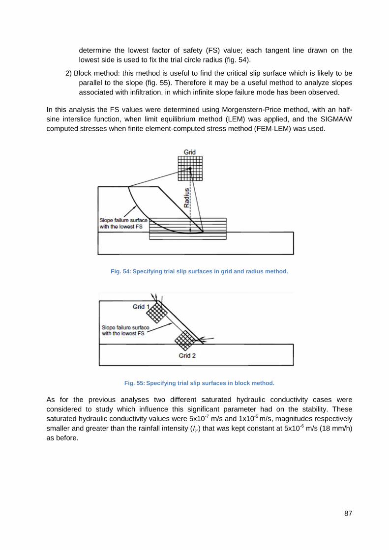
87

determine the lowest factor of safety (FS) value; each tangent line drawn on the lowest side is used to fix the trial circle radius (fig. 54).

2) Block method: this method is useful to find the critical slip surface which is likely to be parallel to the slope (fig. 55). Therefore it may be a useful method to analyze slopes associated with infiltration, in which infinite slope failure mode has been observed.

In this analysis the FS values were determined using Morgenstern-Price method, with an half-sine interslice function, when limit equilibrium method (LEM) was applied, and the SIGMA/W computed stresses when finite element-computed stress method (FEM-LEM) was used.

Fig. 54: Specifying trial slip surfaces in grid and radius me thod.

Fig. 55: Specifying trial slip surfaces in block method.

As for the previous analyses two different saturated hydraulic conductivity cases were considered to study which influence this significant parameter had on the stability. These saturated hydraulic conductivity values were 5x10-7 m/s and 1x10-5 m/s, magnitudes respectively smaller and greater than the rainfall intensity (æK) that was kept constant at 5x10-6 m/s (18 mm/h) as before.

88

7.2. Results

7.2.1. Homogenous Soil Case

Firstly an homogenous soil embankment was assumed. When it was considered the soil bank with an high saturated conductivity value (�� = 1x10-5 m/s), so when the permeability was higher than the rainfall rate (æK), it was not found a real advantage for using the finite element-computed stress method (FEM-LEM) instead of the traditional limit equilibrium method (LEM). The saturation condition was reached in a relatively short time (34 hrs = 1,42 days), as shown in fig. 56, and the most critical slip surface shape and position, at the end of the analysis (60 hrs), was nearly the same for both methods (fig. 57). Nonetheless the safety factor values was different: FS = 1,440 for the FEM-LEM approach; FS = 1,190 for the LEM approach.

Fig. 56: changing position of water table in the ba nk subjected by a constant 5x10 -6 m/s (18 mm/h) rainfall.

89

Fig. 57: Critical slip surface and factor of safety with LEM approach (above) and FEM-LEM approach (bel ow) at the end of the analysis (60 hours). (Ksat = 1e-5 m/s)

The reason for the difference in the safety factor is primarily related to the stress distribution along the slip surface. The FEM-LEM approach was able to capture localized shear stress concentrations that the LEM approach, which derives the slice base normal force only from the slice weight, could not do. This can be observed plotting the shear strength and the mobilized shear stress along the slip surface for the two cases (fig. 58 a) and b)). With the FEM-LEM approach it could be distinguished an area below the crest of the embankment where the soil reached the failure, even if the slope is yet stable as whole. The same was not possible with the LEM approach because it calculate the stresses on each slice that make the factor of safety the same for each slice, regardless to the actual ground stresses. In fact in the graph (fig. 58 b)) the shear strength is everywhere 19% higher of the shear mobilized, irrespective of the considered wedge. Therefore, even if the LEM approach usually gives back a conservative result in term of safety factor (FS) for an high hydraulic conductivity soil case, nevertheless the FEM-LEM approach should be taken into consideration when the problem analysis concerns with the knowledge of the actual ground stresses distribution along the slip surface.

90

Fig. 58: a) shear strength and the mobilized shear stress along the slip surface obtained with FEM-LEM approach; b) shear strength and the mobilized shear stress along the slip surface obtained with LEM

approach;

Passing to analyze the case of lower hydraulic conductivity (�� = 5x10-7 m/s), it was observed that the critical slip surfaces obtained with the limit equilibrium method (LEM) and the finite element-computed stress method (FEM-LEM) were different. As example, using the ‘grid and radius’ method to search the slip surfaces, it was observed that LEM gave back a critical surface always located on the lower part of the slope throughout the time of the analysis, while

0

5

10

15

20

25

0 2 4 6 8 10 12 14

Sh

ea

r R

esi

tan

ce [

kP

a]

Distance X [m]

a)

Shear strength

Mobilized shear stress

0

5

10

15

20

0 2 4 6 8 10 12

Sh

ea

r R

esi

tan

ce [

kP

a]

Distance X [m]

b)

Shear strength

Mobilized shear stress

91

the FEM-LEM gave back a critical surface located on the upper part of the bank (near the crest) where the higher shear stresses were developed as previously illustrated in fig. 50. The fig. 59 reports the grid of rotation centers and the radius lines used to define the slip surfaces. In figs. 60-61 it is showed the critical slip surface after 24 hours from the beginning of the analysis obtained with LEM and FEM-LEM approach, respectively.

Fig. 59: the grid and the radius lines used to defi ne the slip surfaces.

Fig. 60: Critical slip surface and factor of safety with LEM approach after 24 hours. (Ksat = 5e-7 m/s )

92

Fig. 61: Critical slip surface and factor of safety with FEM-LEM approach after 24 hours. (Ksat = 5e-7 m/s)

The critical slip surface found with LEM approach (fig. 60) was always located in the lower part of the slope because, in that zone, to an increasing of water table, due to rainfall infiltration, corresponded an increase of the weight (so of the driving force) and a reduction of the shear strength due to the loss of suction and to the increase of pore-water pressure �� (reduced strength available). So generally, using LEM approach, a slip surface passing across the saturated zone is characterized by a lower safety factor (FS) respect that of another surface drawn entirely inside the partially saturated zone, regardless the shear stress concentrations occurring in the soil. However the problem of an unsaturated soil bank suffering rainfall infiltration is a dynamic situation involving displacements which accumulates in time. Nonetheless the limit equilibrium method of slices does not keep into consideration strains and displacements. Fig. 62 shows the Y-displacements growth in time occurred just below the surface (blue dots): as notable the greatest displacements were in the zone near the crest. The finite element-computed stress method (FEM-LEM) can take into account this fact. It uses the actual SIGMA/W computed stresses to calculate safety factors; therefore it allows to consider actual localized shear stress concentrations caused by the process of water infiltration. In this framework it could be explained why of the critical slip surface position found with FEM-LEM approach (fig. 61): the upper part of the embankment was that characterized by the greatest shear stresses, as showed in fig. 50, and greatest displacements (fig. 62).

93

Fig. 62: Y-displacements at different elapsed times (above) calculated for the points indicated by the blue dots in the scheme (below).

Worth noting is also the fact that LEM approach is based purely on the principle of statics: it finds the forces acting on each slice so that the slice is in force equilibrium and, at the same time, the factor of safety is the same for each slice. As result the computed slice forces can be locally not realistic or representative of the actual in-situ conditions. Conversely the safety factor calculated with FEM-LEM method is not the same all along the slip surface but it can vary, indicating which area is more stressed. Focusing on the second approach (FEM-LEM), it was studied how:

1) the definition of different slip surface search methods have influence on safety factor, and

2) the definition of different radius lines have influence on the shape of the critical slip surface.

Firstly the FEM-LEM stability analysis was carried out employing the ‘grid and radius’ and ‘block’ method. The ‘grid and radius’ method is based on the definition of one grid of circle centers and one radius lines box. The configuration used in the analysis was that shown in fig. 59. Conversely the ‘block’ method can be performed specifying two grids of points and two ranges of projection angles; the slip surface consists of three line segments: the middle segment goes from each grid point on the left to each grid point on the right, while the other two segments are projections to the ground surface at a range of specified angles. The configuration used in the

0

0,0005

0,001

0,0015

0,002

0,0025

0,003

0 5 10

Y-d

isp

lace

me

nt

[m]

X [m]

0 hrs

12 hrs

24 hrs

36 hrs

48 hrs

60 hrs

94

analysis is shown in fig. 63: the two grids of points were plotted over the area, near the surface, where the X-Y shear stresses are higher (see contours in fig. 63).

Fig. 63: grids of points and projection angles (ind icated by the arrows) used in the ‘block’ method (l eft); X-Y shear stress contours at the end of the analysis for the Ksat=5e-7 m/s case (right).

The results, obtained assuming in both cases a slip surface close to the slope face, are illustrated in figs. 64-65.

Fig. 64: Critical slip surface and factor of safety at the end of the analysis (60 hours) – ‘Grid and Radius’ method

Fig. 65: Critical slip surface and factor of safety at the end of the analysis (60 hours) – ‘Block’ me thod

95

The value of FS was lower for the ‘grid and radius’ method (FS=3,094) than for ‘block’ method (FS=3,231); meaning that ‘grid and radius’ was more efficient than ‘block’ method to find the most critical slip surface and it seemed to provide better results. Furthermore it may be stated that regular circular slip surfaces are more likely to occur than a surface formed by multi-straight lines; however it must be remembered that the analysis deals with an homogeneous soil bank; actually, the random spatial variability of soil properties often may result in irregular slip surfaces, as that found with the ‘block’ method. Nevertheless, hereinafter the ‘grid and radius’ method will be considered as it is easier and it has demonstrated to give back results from the side of safety. Then the influence of different radius lines definition on the shape of the critical slip surface was studied. The same stability analysis (FEM-LEM approach and grid and radius method) was performed specifying two different radius lines boxes (fig. 66 a) and b)): one radius lines box was closer to the surface (a), while the other one went deeper into the bank (b).

Fig. 66: two different radius lines configurations: closer to the surface (a) and deeper into the bank (b).

It was found that, in the first case (a case), the critical slip surface was tangent to the radius line closest to the surface (fig. 67), indicating a possible shallow landslide as expectable from the found shear stress contour lines; in the second case (b case) the critical slip surface tends to be tangent to the deeper radius line (fig. 68).

96

Fig. 67: Critical slip surface and factor of safety at the end of the analysis (60 hours) resulting in the a) case.

Fig. 68: Critical slip surface and factor of safety at the end of the analysis (60 hours) resulting in the b) case.

In the figs. 69-70 are reported the variation of the safety factor with time calculated for the two critical slip surfaces illustrated in figs. 67-68, respectively. The two behaviors were rather different. For the a) case there was a sudden decrease of the safety factor corresponding to the loss of the contribution to shear strength provided by soil suction. The rapid decrease was a direct consequence of the high infiltration rate that occurred at the beginning of a rainfall event as showed in Chapter 5 ‘Rainfall Infiltration Analysis’. For the b) case the decrease was more steady because the water took more time to reach the deeper slip surface. Nevertheless the safety factors was lower than for the a) case: at the end of the analysis it was 2,211 for the b) case, while it was 3,094 for the a) case. The reason can be explained looking at the geometry and position of the slip surfaces: the deeper slip surface involves greater destabilizing force; furthermore it is mostly located below the saturated zone meaning greater pore-water pressure (��), greater weight and null suction component of strength.

97

Fig. 69: variation of the safety factor with time f or the critical slip surfaces of the a) case.

Fig. 70: variation of the safety factor with time f or the critical slip surfaces of the b) case.

This fact can be better appreciated plotting the strength component along the slip surface (figs. 71-72). For the shallower slip surface, represented by the a) case, the greatest contribution was provided by the soil cohesion, that was specified to be 5 kPa uniformly throughout the bank; while the suction provided strength is almost reduced to zero at the end of the analysis. For the deeper slip surface, represented by the b) case, the greatest contribution was provided by the frictional property of the soil, while the cohesion had a minor influence; the suction provided strength was present only along the upper slices, where there was not saturated condition yet.

Fac

tor

of S

afet

y

Time (sec)

3

3.5

4

4.5

5

0 50000 100000 150000 200000 250000

Fac

tor

of S

afet

y

Time (sec)

2.2

2.3

2.4

2.5

2.6

2.7

2.8

0 50000 100000 150000 200000 250000

98

Fig. 71: Strength components along the slip surface for the a) case.

Fig. 72: Strength components along the slip surface for the b) case.

7.2.2. Non-homogenous Soil Case

If it is supposed that the most shallow soil layer is influenced by the weathering and by the repeated wetting-drying cycles, than the hypothesis of homogeneous soil strength parameters may not be valid anymore. About the atmospheric agents (weathering) the following can be reminded:

− physical weathering:

• heat: repeated heating and cooling exerts stresses on the outer layers.

0

2

4

6

8

10

12

0 5 10 15 20

Str

en

gth

[k

Pa

]

slice number

Frictional

Cohesive

Suction

Total Shear Strength

0

5

10

15

20

25

30

0 5 10 15 20

Str

en

gth

[k

Pa

]

slice number

Frictional

Cohesive

Suction

Total Shear strength

99

• water: the action of both rain and runoff contributes to disaggregation of the soil; usually embankments subjected to repeated wetting and drying cycles are characterized by movements and deformations of surficial layer, especially if the clayey content is significant and shrinking and swelling occur.

• frost: freezing and thawing cycles are among the most severe causes of cracks and fissures formation on soil.

− chemical weathering:

• dissolution, carbonation, hydration, oxidation, hydrolysis on silicates and carbonates: all these represent a minor cause of disaggregation for a soil because they act primarily on the rocks, however their contribution may become significant if the minerals content of the soil are sensible to these chemical actions.

− biological weathering:

• plants: the roots growth can improve the stability in some cases, or produce fissures along which weak slip surface are created.

• animals: some animal burrow hollow in the soil.

Cracks and fissures (disaggregation) produced by weathering may cause a reduction of the soil strength parameters, especially of cohesion. Moreover the accumulation of shear and volumetric deformation induced by cyclic occur of the rainfall and other atmospheric agents (which induce cyclic oscillations of shear and mean effective stresses) may contribute to the decrease of cohesion, leading to a progressive failure in the shallower part of the soil bank (Cola et al. (2008)). The materials most likely to exhibit progressive failure are the finer materials (such as clays) because they possess chemical bonds that are gradually disintegrated by weathering. To take into account the effect of strains on this superficial shear band of the soil, the strengths should be scaled by a factor that depends on the strain rate. Nowadays this is not achievable with Geostudio softwares. However SLOPE/W can account these alteration phenomena specifying a spatial function for cohesion (c) as function of both x and y geometry coordinates. Therefore a new analysis was performed considering the same bank as before but using a spatial function for cohesion. Cohesion was kept constant (equal to 5 kPa) inside the bank, while it was supposed to vary linearly between 5 kPa to 0 kPa within the most shallow 0,50 m layer from the ground surface, where the fissures and cracks were supposed to develop. In fig. 73 are shown the contours of the actual applied cohesion values.

100

Fig. 73: contours of the actual applied cohesion va lues.

With this strength parameter configuration, the critical slip surfaces obtained, at the end of the analysis (60 hours), for the two different radius lines box specified (case a) and b)) are reported in fig. 74.

Fig. 74: Critical slip surface and factor of safety at the e nd of the analysis (60 hours) resulting in the a) a n b) case, with a spatial function for cohesion defined.

It could be noted that now the safety factor of the a) case was significantly reduced respect the previous analysis: before it had reached a value of 3,094; now it was 2,115. This means that a narrow soil band characterized by a little range of variability for cohesion strength component, can yield large differences in stability results. Also more interesting was that, unlike what happened before, now the safety factor was lower for the a) case (FS=2,115) than for b) case (FS=2,168). In fig. 75 it is reported the variation of the safety factor with time calculated for the two critical slip surfaces. For the a) case there was a sudden decrease of FS, like before, but now FS values were lower and the a) curve crossed that of the b) case. After this point, in which the curves crossed each other, it can be stated that shallow failures occur prior to deep failure. Obviously the FS decreasing rate is a function of the rainfall intensity, the hydraulic conductivity function, the initial degree of saturation in the soil and the geometry; a parametric study based on their variation should be performed (see Chapter 8 ‘Parametric Study’).

101

Fig. 75: variation of the safety factor (FS) with ti me for the critical slip surfaces of the a) case an d b) case , with a spatial function for cohesion defined.

Cracks and fissures have influence not only on the strength parameters but mainly on hydraulic conductivity. In natural slopes the saturated hydraulic conductivity of earth materials for texturally similar materials commonly can vary over one to two orders of magnitude, as found by Reid ME. (1997). This contrasts in the hydraulic conductivity can greatly modify the pore-pressure distribution, elastic effective-stress field, and stability within the slope. Reid ME. (1997) performed a study, with a finite-element numerical model, analyzing four simple hillslope configurations with layered materials having different ��. It was assumed fully saturated, ground-water flow. He found that low hydraulic conductivity materials that impede downslope ground-water flow can create unstable areas, with locally elevated pore-water pressures and seepage forces, that are quite different from the homogeneous case. The destabilizing effects can be as great as those induced by a variation in the frictional strength of approximately 4° - 8° (for the case examined) of texturally similar materials. In this analysis there was not fully saturated flow conditions throughout the embankment but anyway much attention should been paid to examine the destabilizing effect caused by variation in hydraulic conductivity. Fissured shallow layers of constructed embankments can have permeability and shear strength which vary gradually with depth, controlling both local seepage response to rainfall infiltration and location of the critical shear surface. Therefore it was performed a new analysis which combined the definition of a spatial cohesion function with the presence of a shallow layer with higher hydraulic conductivity. The previous idealized soil bank with a height of 5 m was divided into two layers: (Layer 1) a shallow layer with approximately 0,4-0,5 m thickness, and (Layer 2) the remaining soil volume, as shown in fig. 76. The two layers had two saturated hydraulic conductivities: �� = 1x10-5 m/s for Layer 1, and �� = 5x10-7 m/s for Layer 2. The rainfall rate (æK) considered was always 5x10-6 m/s (18 mm/h). Therefore, in relation to Layer 2, the infiltration rate was greater than the infiltration capacity (æK ¦ ��); in this sense the analysis can be seen as a study on the real effect of heavy rainfalls on bank stability. In fact the high hydraulic conductivity of Layer 1 is not an original feature of the embankment but it represents the effect on medium-long term of weathering action.

1,5

2

2,5

3

3,5

4

4,5

5

0 20 40 60

Fa

cto

r o

f S

afe

ty (

FS

)

Time (hours)

a) case

b) case

102

Fig. 76: Non-homogeneous soil bank mesh with 2 layers.

The results of this non-homogeneous case were compared with those previously obtained from the homogeneous soil case. The same mesh-points (point A-B in fig. 77) are considered when results are illustrated.

Fig. 77: representative point A and B on the finite element domain

In fig. 78 are presented the time histories of matric suction, for point A, obtained from the two homogeneous cases (�� = 1x10-5 m/s and �� = 5x10-7 m/s) and the new non-homogeneous case (�ç�J\ = 5x10-7 m/s and �ç�J> = 1x10-5 m/s). As notable for the new non-homogeneous

case there was the most sudden matric suction decrease. The Layer 1 of the non homogeneous case was assumed to have the same permeability of the first homogeneous case (�� = 1x10-5 m/s) indicated with the blue curve in fig. 78; however the presence of the Layer 2, with lower conductivity, prevented the drainage of the water so that suction was sudden reduced to zero, even more rapidly than for the ‘�� = 5x10-7 m/s homogeneous’ case (red curve). This noticeable drop of matric suction inside the top layer could lead to slope instability featured by shallow failures.

103

Fig. 78: time histories of matric suction at point A

In fig. 79 are presented the time histories of matric suction obtained for point B. When there was a greater distance from the slope surface, the matric suction of a soil with high hydraulic conductivity decreased more quickly than that with low conductivity, as shown by the blue and red curves. The non-homogeneous curve was located in the middle of the two extreme homogeneous cases; after all, being B a point still quite closer to the surface, the green curve is near the blue one since it still suffers the presence of the high hydraulic conductivity Layer 1; as the distance increases the influence of Layer 1 will weaken and the green curve will approach the red one.

Fig. 79: time histories of matric suction at point B

Upon completion of the above results on suction obtained by transient seepage analyses, the corresponding slope stability of the bank, for the same time interval (60 hours), was examined

0

5

10

15

20

25

30

35

40

0 20 40 60

Su

ctio

n [

kP

a]

Time [hours]

Ksat = 1e-5 m/s (homogeneous)

Ksat = 5e-7 m/s (homogeneous)

Klay2 = 5e-7 m/s , Klay1 = 1e-5 m/s

(non-homogeneous)

0

5

10

15

20

25

30

35

0 20 40 60

Su

ctio

n [

kP

a]

Time [hours]

Ksat = 1e-5 m/s

(homogeneous)

Ksat = 5e-7 m/s

(homogeneous)

Klay2 = 5e-7 m/s , Klay1 = 1e-

5 m/s (non-homogeneous)

104

using the finite element-computed stress method (FEM-LEM) in SLOPE/W. It is remembered that the non-homogeneous bank case is characterized by a superficial layer (Layer 1) with higher permeability then the remaining soil (Layer 2), and by spatial varying values for cohesion (a spatial function for cohesion is defined). The most surprising fact was that, for the first time, the same critical slip surface was obtained at the end of the analysis for both the ways to specify the radius lines (case a) and b)) as illustrated in fig. 80. Therefore it can be stated that when details, which represent actual field conditions, are included in the stability analysis then a single critical slip surface is obtained, regardless the way to specify slip surfaces (in particular, the radius lines box if ‘grid and radius’ method is applied). Here, in this analysis, the details specified were:

− the spatial function for cohesion, in order to account for lower cohesion strength near the surface produced by weathering;

− the surficial Layer 1 with higher permeability, in order to account the effect of fissures and cracks;

Other peculiarities may be included in the future studies.

Fig. 80: Critical slip surface at the end of the a nalysis (60 hours) resulting in the a) case (left) and b) case

(right).

Fig. 81 shows the critical slip surface found for the embankment with lower hydraulic conductivity (�� = 5x10-7 m/s), together with the variation of the factor of safety (FS) with time, under different degrees of specification.

105

Fig. 81: (above) critical slip surface at the end o f the analysis for the embankment with lower hydraulic conductivity ( ÌÍÎÏ = 5x10-7 m/s); (below) variation of

the factor of safety (FS) with time, under different degrees of specification;

The differences between the three cases are significant: more the actual details are included in the analysis and the lower is the safety factor. In the Table 5 are reported the FS values for the three cases at the end of the analysis and the rate of change respect the homogeneous case. Large part of the decrease occurred in a short time, less than 20 hours. It is reminded that the rainfall rate is kept always equal to 5x10-6 m/s (18 mm/h) throughout all the analysis. Therefore the results obtained can be seen as the effects of long-duration, high-intensity (18 mm/h) events on the stability of a soil embankment; the reduction of suction, due to water infiltration, is reflected in the decrease of the modeled factor of safety from higher values (around 5,0) to lower values, just above unity in some cases.

Table 5: the FS values for the three cases at the en d of the analysis and the rate of change respect the homogeneous case

FS rate of change

Homogeneous K sat = 5e-7 m/s 3,094 /

Homogeneous K sat = 5e-7 m/s,

with spatial function for cohesion 2,115 -31,6 %

Non-homogeneous (K lay 1 = 1e-5 m/s, K lay 2 = 5e-7 m/s), with spatial function for cohesion

1,505 -51,4 %

7.3. Conclusions

The results here presented confirm as follow:

1. The rainfall infiltration causes the slope soil matrix suction to decrease, or even disappear, differently in time according to the hydraulic permeability, and this is also reflected by the reduction of the safety factor (FS).

0

1

2

3

4

5

6

0 20 40 60

Fa

cto

r o

f S

afe

ty (

FS

)

Time (hours)

homogeneous Ksat = 5e-7 m/s

homogeneous Ksat = 5e-7 m/s , with

spatial function for cohesion

non-homogeneous (Klay1 = 1e-5 m/s ,

Klay2 = 5e-7 m/s ) , with spatial

function for cohesion

106

2. Under the dual role of matrix suction reduction and transient water load increasing, the critical slip surface can be evaluated with different limit equilibrium approaches. For the higher permeability soil, the shape and location of the critical slip surface is nearly the same with the two experimented approaches but the lower FS is found with the LEM one; nonetheless, the FEM-LEM approach is able to provide additional interesting knowledge about the distribution of the shear stresses along the slip surface. For the lower hydraulic permeability soil, instead, the FEM-LEM approach is the only able to reveal a slip surface which con take into account the localized high stressed zones induced by the infiltration process; particularly the higher stresses were found to occur in the upper part of the slope, near the crest.

3. If details representing actual field conditions (as the reduction of cohesion strength and the increase of permeability near the surface due to the weathering processes) are included in the stability analysis, then one critical slip surface is obtained uniquely, regardless the way to specify slip surfaces. Moreover it was observed a reduction of the safety factor, at the end of the analysis, as much as 50%.

Therefore, errors may arise when the traditional limit equilibrium method (LEM) is used to estimate the safety factor of slope’s banks subjected to rainfall infiltration, with a permeability less than the rainfall rate. The analysis indicate that often the use of the common LEM approach lead to wide critical slip surfaces including both locally failed regions; or it can led to critical slip surfaces always located in the lower part of the bank (near the toe), mainly below the water table. In this way it neglects the stresses and deformations caused by rainfall in the upper part of the embankment, near the crest. Namely, since the local failures near the slope surface can be overlooked, the safety factor may be overestimated (non-conservative). In effect, the superficial local failure of a slope embankment may not led to instantaneous overall collapse. However, once a local zone fails, the region can propagate in depth toward areas where the shear strength is exceeded until a global slide activates. Therefore, it should be mentioned that local failures can no longer be neglected in transient stability analysis, since the soil near the surface may be saturated from rainfall and the strength may be temporarily decreased during the event. The numerical simulations of this thesis provide an initial understanding of the actual mechanism of soil slope instability for transient conditions leading to shallow surface failure caused by rainfall infiltration.

107

Chapter 8

Parametric Study

8.1. Introduction

In this study the stability of the bank was assessed through the factor of safety (dependent variable) and the other factors (independent variables) affecting the stability of a slope. The latter were considered to be the soil properties, rainfall intensity, the slope geometry (slope angle) and the initial moisture condition. In a first analysis three slope angles (26.6, 33.7, and 45.0°), two soil types (namely two saturated hydraulic conductivity values: �� = 5x10-7 m/s and �� = 1x10-5 m/s), and four rainfall intensities (æK) (3, 6, 12, 18 mm/h each for 24 h duration) were used to perform the parametric study. Thus, with this combination, 24 (3 x 2 x 4) analyses were performed where the slope height (5,0 m) and the initial groundwater table position (at the bottom of the embankment) were kept constant throughout all the analysis. The initial pore-water pressure condition, for all the analyses, was a hydrostatic condition with a limiting pore-water pressure head of −5 m. This was done to eliminate the effects of antecedent moisture conditions on the factor of safety of the slope. This first study was intended to evaluate the effect of soil properties, in terms of saturated coefficient of permeability (�� ), and the effect of slope angle on the stability of a homogeneous soil slope subjected to different rainfall rates. A second parametric study was carried out to investigate the effect of rainfall intensity on the factor of safety (FS), and the existence of a threshold rainfall intensity which would cause the maximum reduction in the FS. A fixed 45° slope angle bank was considered, while it was varied the soil type (two cases: �� = 5x10-7 m/s and �� = 1x10-5 m/s) and the rainfall intensity (13 different values, each for 24 h duration); overall 21 analyses were performed. A last parametric study was carried out to looking for the influence that antecedent moisture condition (or antecedent rainfall) have on the stability of the ‘�� = 5x10-7 m/s homogeneous soil bank’. Again, a fixed 45° slope angle bank was taken as example, while three rainfall intensities (3, 6 and 12 mm/h, each one maintained until failure onset) and five initial relative degree of saturation (�Z) were varied. Overall 15 analyses were performed. Table 6 gives a summary of the combination of factors controlling slope stability that were varied and kept constant in the three different series of parametric studies. Each parametric study was performed in three steps. First, a seepage analysis of the homogeneous soil bank was performed using SEEP/W software. The pore-water pressures obtained from the seepage analysis are then used in an uncoupled consolidation analysis (SIGMA/W software) to calculate the stresses and the deformations. Finally, with SLOPE/W software, a slope stability analyses to calculate the factor of safety (FS) of the slope’s bank was performed using the finite element-calculated stress method (FEM-LEM).

108

Table 6: summary of combination of factors (independent vari ables) affecting slope stability used in parametric studies.

Study Name Soil type - ÌÍÎÏ [m/s]

Slope angle α [°]

Rainfall intensity èé [mm/h]

Initial relative

degree of saturation �ê [%]

Number of combination

‘Slope angle and Rainfall

Intensity’

5x10-7 1x10-5

26,6 33,7 45,0

3 6 12 18

24

‘Threshold Rainfall

Intensity’

5x10-7 1x10-5

45,0

0,5 1 2 3 6 9

12

15 18 22 26 30 60

21

‘Antecedent Rainfall’

5x10-7 45,0 3 6 12

0,64 0,73 0,80 0,90 0,98

15

The shear strength equation utilized in the slope stability analysis is the unsaturated shear strength equation to incorporate the contribution from the negative pore-water pressure. The equation is that proposed by Fredlund et al.(1978), which can be expressed as follows:

V" � � � �� tan � � �� tan ��

where V" is the shear stress at failure for unsaturated soils, c′ and φ′ are effective shear strength

parameters (the effective cohesion and friction angle), � is the normal stress on shear surface, �� is a friction angle related to matric suction �� , �� and �� are respectively the pore air and pore-water pressure. The shear strength parameters and mechanical properties of the soils used in the parametric studies were the same of the previous analyses, and these are recalled in Table 7.

Table 7: Materials properties and shear strength pa rameters for the soil considered in the FEM parametric analysis

Material properties Symbol Unit Value

Unit weight of soil kN/m3 20

Young’s modulus N kPa 10000

Poisson ratio ë / 0,27

Saturated hydraulic conductivity �� m/s 1e-5 and 5e-7

109

Cohesion intercept �’ kPa 5

Internal friction angle �′ ° 30

Matric suction angle �� ° 15

To take into account the effect of weathering on superficial layer, a spatial function for cohesion was used as for the previous ‘slope stability analysis’. The apparent cohesion strength was imposed to vary linearly from 0 kPa to 5 kPa inside the most shallow 0,4 – 0,5 m thick soil layer (fig. 82).

Fig. 82: contours of the actual applied cohesion va lues.

Instead, the influence of weathering on hydraulic conductivity was neglected here, and the bank was assumed homogeneous from the permeability point of view.

8.2. Results and Discussion

8.2.1. Slope Angle and Rainfall Intensity

The effect of slope angle (α) and the rainfall intensity (æK) on the stability of a homogenous soil slope with saturated hydraulic conductivities �� = 5x10-7 m/s and �� = 1x10-5 m/s, is shown in figs. 83-84, respectively. The plots in figs. 83-84 highlight the relationships of the initial factor of safety, ��3�3, and the minimum factor of safety, ��Y3�, with slope angle (α) for all the rainfall intensities (æK) examined. The plots show a common pattern for the minimum factor of safety, ��Y3�, irrespective of the soil type and slope angle: where the higher the rainfall intensity the lower the ��Y3�. This implies that the rainfall intensity plays a primary control on safety factor (FS). A comparison of the plots among the same soil type but different slope angles (so looking at figs. 83-84 separately) indicated that the higher the slope angle the lower the initial factor of safety, ��3�3, and the minimum factor of safety, ��Y3�: both ��3�3 and ��Y3� bore negative linear relationship with α. This is conceivable because a steep slope will yield a lower factor of safety (FS) as compared to a flat slope. Therefore, also the slope angle plays an important role in dictating the FS of the slope. Again, comparing the results plotted in figs. 83-84, it was noted that under a short-duration rainfall (Tí î24 h) the trend lines were stepper for the low permeability (K��Ò = 5x10-7 m/s) homogeneous soil bank than for the high permeability (K��Ò = 1x10-5 m/s) one. For the lower permeability soil (fig. 83), at the higher slope angles (α = 45.0°) and rainfall intensities (æK) between 6 and 18 mm/h, the minimum safety factor it was observed approaching dangerously

110

to the limit value (FS = 1); and, observing the trend line, for slopes beyond the 50° with a rainfall intensity equal or greater 12 mm/h the FS limit may be exceeded probably. The same was not observed in fig. 84 (high permeability, K��Ò = 1x10-5 m/s, homogeneous soil bank) where the FSð�� values were always greater 1,5 even for the highest slope angle (α) and rainfall intensity (Ií). At the lower slope angles, the trend lines in fig. 83 are quite spaced each other, while those in fig. 84 are quite close to one another. This means that a soil bank with a saturated coefficient of permeability �� = 1x10-5 m/s was less influenced by the variability of rainfall intensity. Contrarily, soil bank with �� value of 5x10-7 m/s was greatly affected by rainfall intensity variability.

Fig. 83: Relationship between slope angle ( α) and minimum factor of safety, ñ�òóô, for homogeneous soil bank ( ÌÍÎÏ = 5x10-7 m/s) subjected to rainfall for 24 h with four rain fall intensities of 3, 6, 12 and 18 mm/h.

0

1

2

3

4

5

6

20 30 40 50 60

Min

imu

m s

afe

ty f

act

or,

FS

min

Slope angle, α (°)

FS ini

Ir = 3 mm/h

Ir = 6 mm/h

Ir = 12 mm/h

Ir = 18 mm/h

FS lim

Trend line

111

Fig. 84: Relationship between slope angle ( α) and minimum factor of safety, ñ�òóô, for homogeneous soil bank ( ÌÍÎÏ = 1x10-5 m/s) subjected to rainfall for 24 h with four rain fall intensities of 3, 6, 12 and 18 mm/h.

The above findings suggest that homogeneous soil slopes with a low saturated coefficient of permeability (�� = 5x10-7 m/s) are not safe from short-duration rainfalls, contrary to what was stated by Rahardjo, Harianto, et al. (2007), where a short-duration rainfall is defined as the “1 day” or “24-h” rainfall. In fact, using the FEM-LEM approach it was possible to take into account the stresses produced by rainfall infiltration on the superficial layer, while the LEM could not do this. In case of low conductivity soil (�� = 5x10-7 m/s), the effect of the infiltration results in a critical slip surface close to the surface which is characterized by lower safety factor than that of the high conductivity soil case (�� = 1x10-5 m/s) which is seated more in deep. What had not been caught by Rahardjo, Harianto, et al.(2007) was, probably, the different ways in which different hydraulic conductivity soil slopes fail when subjected to a rainfall infiltration; in fact the LEM approach does not allow to recognize these differences. Another important thing to note in the above fig. 83 is that the ��Y3� value points found for æK = 12 mm/h and æK = 18 mm/h were almost the same: the point tend to overlap each other. This

suggests the possibility of the existence of a threshold rainfall intensity which will cause the maximum reduction in ��Y3� of a homogeneous soil slope.

8.2.2. Threshold Rainfall Intensity

To investigate the existence of a threshold rainfall intensity in more detail, and to examine the relationship between minimum factor of safety (��Y3�) and rainfall intensity (æK), the minimum factor of safety versus logarithmic of rainfall intensity, for an α = 45° slope soil bank, is plotted in fig. 85, for �� = 5x10-7 m/s and �� = 1x10-5 m/s soil cases. Other values of rainfall intensities were added to those previously investigated in order to obtain a more accurate curve relationship. The semilog plots, in fig. 85, shows that generally the FSð�� and Ií relationship follows a sigmoid shape which suggests the existence of an upper and a lower inflection point.

0,5

1

1,5

2

2,5

3

3,5

20 30 40 50 60

Min

imu

m s

afe

ty f

act

or,

FS

min

Slope angle, α (°)

FS ini

Ir = 3 mm/h

Ir = 6 mm/h

Ir = 12 mm/h

Ir = 18 mm/h

FS lim

Trend line

112

For the lower hydraulic conductivity soil case (�� = 5x10-7 m/s) the ��Y3� tended to be almost constant at very low rainfall intensities, approximately below æK = 2-3 mm/h (upper inflection point). Then, after this upper inflection point, the ��Y3� started to decrease rapidly until it was reached a threshold rainfall intensity value (lower inflection point) after which the ��Y3� remained constant. This threshold value, for the �� = 5x10-7 m/s case, was around æK = 10 mm/h. The same analysis repeated for the �� = 1x10-5 m/s case revealed an upper inflection point which could be estimated around æK = 10 mm/h, higher respect that of �� = 5x10-7 m/s case; and it was found as threshold rainfall intensity (lower inflection point) a value æK = 30 mm/h. A comparison among the two different soil types considered here demonstrated that higher the conductivity (��) higher were the upper and lower inflection point values. This implies that, in order to bring the ��Y3� to its lowest value, a higher rainfall intensity (æK) is needed in a homogeneous soil bank with a high permeability (�� = 1x10-5 m/s) than in a homogeneous soil bank with a low permeability (�� = 5x10-7 m/s). The existence of a threshold rainfall intensity means also that the reduction of safety factor (FS) is only significant until it is reached the return period of that threshold rainfall intensity. A further increase in the return period will not produce any decrease in the safety factor. Therefore much attention should be paid to banks with low �� soils since also very common events, with low return period, can lead to failures.

Fig. 85: relationships between rainfall intensity ( èé) and minimum factor of safety, ñ�òóô, for the two homogeneous soil bank ( ÌÍÎÏ = 5x10-7 m/s and ÌÍÎÏ = 1x10-5 m/s) with slope angle α=45°,

subjected to rainfall for 24 h.

Reasoning in terms of water volume, it can be stated that homogeneous soil banks need more water to destabilize if the �� is high than if the �� is low. The reason is that the mechanisms of failure are different for the two cases. Soil banks with low �� usually destabilize due to rainwater infiltration that causes, in short time, the reduction of matric suction shear strength component in the superficial unsaturated zone (shallow failures). Instead soil banks with high �� usually fail under more intense rainfalls, due to the increase of pore-water pressure �� in the inner areas of the embankment (deep seated failures) since the soil can readily drain down

0

0,5

1

1,5

2

2,5

3

0,1 1 10 100

Min

imu

m s

afe

ty f

act

or,

FS

min

Rainfall Intensity, Ir [mm/h]

FS min, homogeneous

soil Ksat = 5e-7 m/s

FS min, homogeneous

soil Ksat = 1e-5 m/s

Slope angle α = 45°

113

the water infiltrating on the surface. So, under low intensity rainfalls, a high �� soil bank will fail only if rain lasts long time.

8.2.3. Antecedent Rainfall

Now it is wanted to bring emphasis to the importance of the antecedent rainfall, or initial moisture condition, in destabilizing the slopes of homogeneous soil bank. In fig. 86 are reported the plots of variation in factor of safety (FS) versus elapsed time for the two different homogeneous soil banks, subjected to different 24 hours-duration rainfall intensities. These plots show that after a rainfall event starts the factor of safety (FS) will drop regardless of the soil type or the rainfall intensity (æK) applied to the slope bank. Only for �� = 1x10-5 m/s and æK = 3 mm/h the rain seems not to affect in any way the stability of the slope bank. Moreover it could be noted that after the rainfall ceased, the factor of safety (FS) for the ��= 1x10-5 m/s soil type recovered at faster rate respect that of the �� = 5x10-7 m/s soil type, and it could reach again the starting condition about 36 hours after the end of the event. Instead the �� = 5x10-7 m/s soil type recovered more slowly toward the initial condition.

0

0,5

1

1,5

2

2,5

3

3,5

0 10 20 30 40 50 60

Fa

cto

r o

f S

afe

ty,

FS

Time [hrs]

Ksat = 5e-7 m/s

Ir = 3 mm/h

Ir = 6 mm/h

Ir = 12 mm/h

Ir = 18 mm/h


114

Fig. 86: Effect of rainfall intensity on variation of factor of safety with time for homogeneous soil slope constant slope angle ( α = 45°) subjected to rainfall for 24 h with: ÌÍÎÏ = 5x10-7 m/s (above);

ÌÍÎÏ= 1x10-5 m/s (below);

The above findings suggest that homogeneous soil bank with a high saturated coefficient of permeability (��= 1x10-5 m/s) are safe from short-duration (24 hours) rainfalls, and seldom they can suffer the influence of antecedent events. For this reason hereafter the effect of the antecedent rainfall will be investigated only for the low hydraulic conductivity case (�� = 5x10-7 m/s soil type). In order to obtain some initial spatial distributions of moisture in the soil, it was think to force the embankment with a cyclic rainfall for eight days (192 hours); it consisted of a constant rainfall lasting 24 hours followed by other 24 hours with no rain, and this repeated for eight days. Four different rainfall intensities were experimented (fig. 87).

0

0,5

1

1,5

2

2,5

3

0 10 20 30 40 50 60

Fa

cto

r o

f S

afe

ty,

FS

Time [hrs]

Ksat = 1e-5 m/s

Ir = 3 mm/h

Ir = 6 mm/h

Ir = 12 mm/h

Ir = 18 mm/h


0,0

2,0

4,0

6,0

8,0

10,0

12,0

14,0

16,0

18,0

20,0

Ra

infa

ll I

nte

nsi

ty,

Ir [

mm

/h]

Time [hrs]

Ir = 3 mm/h,

cyclic rainfall

0,0

2,0

4,0

6,0

8,0

10,0

12,0

14,0

16,0

18,0

20,0

Ra

infa

ll I

nte

nsi

ty,

Ir [

mm

/h]

Time [hrs]

Ir = 6 mm/h,

cyclic rainfall

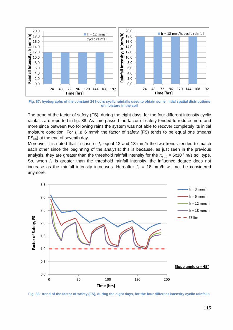
115

Fig. 87: hyetographs of the constant 24 hours cyclic rainfal ls used to obtain some initial spatial distribution s of moisture in the soil

The trend of the factor of safety (FS), during the eight days, for the four different intensity cyclic rainfalls are reported in fig. 88. As time passed the factor of safety tended to reduce more and more since between two following rains the system was not able to recover completely its initial moisture condition. For æK õ 6 mm/h the factor of safety (FS) tends to be equal one (means FSlim) at the end of seventh day. Moreover it is noted that in case of æK equal 12 and 18 mm/h the two trends tended to match each other since the beginning of the analysis; this is because, as just seen in the previous analysis, they are greater than the threshold rainfall intensity for the �� = 5x10-7 m/s soil type. So, when æK is greater than the threshold rainfall intensity, the influence degree does not increase as the rainfall intensity increases. Hereafter æK = 18 mm/h will not be considered anymore.

Fig. 88: trend of the factor of safety (FS), during the eight days, for the four different intensity cyclic rain falls.

0,0

2,0

4,0

6,0

8,0

10,0

12,0

14,0

16,0

18,0

20,0R

ain

fall

In

ten

sity

, Ir

[m

m/h

]

Time [hrs]

Ir = 12 mm/h,

cyclic rainfall

0,0

2,0

4,0

6,0

8,0

10,0

12,0

14,0

16,0

18,0

20,0

Ra

infa

ll I

nte

nsi

ty,

Ir [

mm

/h]

Time [hrs]

Ir = 18 mm/h, cyclic rainfall

0,0

0,5

1,0

1,5

2,0

2,5

3,0

3,5

0 50 100 150 200

Fa

cto

r o

f S

afe

ty,

FS

Time [hrs]

Ir = 3 mm/h

Ir = 6 mm/h

Ir = 12 mm/h

Ir = 18 mm/h

FS lim


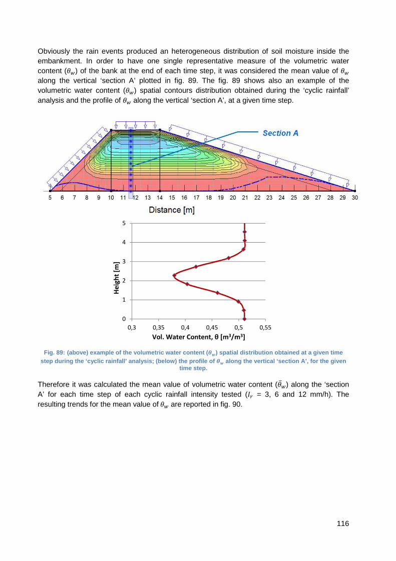
116

Obviously the rain events produced an heterogeneous distribution of soil moisture inside the embankment. In order to have one single representative measure of the volumetric water content (?�) of the bank at the end of each time step, it was considered the mean value of ?� along the vertical ‘section A’ plotted in fig. 89. The fig. 89 shows also an example of the volumetric water content (?�) spatial contours distribution obtained during the ‘cyclic rainfall’ analysis and the profile of ?� along the vertical ‘section A’, at a given time step.

Fig. 89: (above) example of the volumetric water content ( ö÷) spatial distribution obtained at a given time step during the ‘cyclic rainfall’ analysis; (below) the profile of ö÷ along the vertical ‘ section A’, for the given

time step.

Therefore it was calculated the mean value of volumetric water content (?̅�) along the ‘section A’ for each time step of each cyclic rainfall intensity tested (æK = 3, 6 and 12 mm/h). The resulting trends for the mean value of ?� are reported in fig. 90.

0

1

2

3

4

5

0,3 0,35 0,4 0,45 0,5 0,55

He

igh

t [m

]

Vol. Water Content, θ [m3/m3]

117

Fig. 90: trends of the mean vol. water content valu e (øùú) along ‘ section A’ during the ‘cyclic rainfall’ analysis.

As it can be noted a wide range of possible initial moisture conditions was reproduced with the cyclic rainfalls. From the initial condition ?̅� = 0.35, until ?̅� = 0.502, at the beginning of seventh day, which is close to the saturated volumetric water content of the soil ?û = 0.511. Therefore five different moisture conditions has been selected. These were imposed as initial condition for the following analyses in which a steady rainfall is maintained upon the bank until failure was reached (FS=1,0). Three steady rainfall intensities were applied: æK = 3, 6 and 12 mm/h. Varying the rainfall pattern as occurs in actual situations was not attempted: it is beyond the scope of this study.

In order to have a clearer idea of the starting degree of saturation into the soil, the relative degree of saturation (�Z) was calculated for each initial condition:

�Z � ?̅� � ?K?� � ?K

where: ?̅� = mean volumetric water content along the ‘section A’ ?K = residual volumetric water content ?� = saturated volumetric water content

Then, the duration of rainfall needed to reach failure was observed for each initial moisture condition and each steady rainfall. The results are plotted in fig. 91 which reports the rainfall duration until the slope failure as function of the initial mean relative degree of saturation (�Z) along ‘section A’. The trend lines in fig. 91 indicates that the rainfall duration decreased almost linearly with the increase in the initial relative degree of saturation (�Z). Failure took place if the rainfall lasted some hours. How many hours depended on the initial relative degree of saturation (�Z). The lower was �Z the longer the rainfall needed to last until slope failure took place.

0,3

0,35

0,4

0,45

0,5

0,55

0 50 100 150 200

Vo

l. W

ate

r C

on

ten

t, θ

w[m

3/m

3]

Time [hrs]

Ir = 3 mm/h,

cyclic rainfall

Ir = 6 mm/h,

cyclic rainfall

Ir = 12 mm/h,

cyclic rainfall

118

Comparing the three rainfall intensity cases it could be noted that differences occurred only for æK ä 6 mm/h, while for æK = 6 and 12 mm/h the trend lines matched to each other. Moreover the differences reduced progressively as relative degree of saturation (�Z) increased, and when �Z ¦ 80% the three rainfalls gave rise to a unique relationship. As example, if the initial �Z = 90% (which can be considered a common value occurring in actual silty-sandy soils) the failure took place in about 24 hours regardless the rainfall intensity. It must be remembered that here �Z corresponds to the mean value of water content (?̅�) along the vertical ‘section A’, and that a 45° slope angle is considered. Therefore, if another reference is taken or other geometric configurations are investigated, then the relationship curves may be different.

Fig. 91: Effect of initial relative degree of saturation on r ainfall duration until the slope failure

Because the initial relative degree of saturation is significantly influenced by the antecedent rainfalls, these last should be considered in the stability analysis of slope embankments under rainfall. Particularly for those low permeability soils which, as previously seen, are not able to recover fast the initial highly unsaturated moisture conditions. The initial volumetric moisture content has significant influence on the water pressure growth process, and thus on the slope stability. The higher the initial volumetric water content, the higher the hydraulic conductivity and the faster the water pressure raise in soil embankments under rainfall. Li et al. (2005) computed several field measurements on an instrumented cut slope in Hong Kong during the rainy season in 2001, and they observed that the antecedent rainfall infiltration contributed significantly to the increase in volumetric water content and decrease in matric suction, and that the magnitudes of such increase and decrease were dependent on the intensity of the antecedent rainfalls.

0

20

40

60

80

100

120

140

160

0,60 0,65 0,70 0,75 0,80 0,85 0,90 0,95 1,00

Du

rati

on

un

til

the

slo

pe

fa

ilu

re [

hrs

]

Relative Degree of Saturation, Se [%]

Ir = 3 mm/h (data

point)

Ir = 6 mm/h (data

point)

Ir = 12 mm/h (data

point)

Trend (Ir = 3 mm/h)

Trend (Ir = 6 mm/h)

Trend (Ir = 12 mm/h)


119

Chapter 9

Conclusions

In this study the process of water infiltration into a partially saturated model embankment was conducted to investigate the effect of coupled pore water flow and solid skeleton deformation by using two-dimensional finite element software. Rainfalls will increase, depending on the soil's permeability, the soil moisture content, and in turn decrease the matric suction, thus reducing the shear strength of a soil. At the same time the soil mass density will increase, leading to a less stable soil slope. In many cases, in fact, shallow failures, occurring along the slopes embankment, cannot really be attributed to a rise of the groundwater table, but simply to the advance of the wetting front and the reduction of shear strength caused by the decrease of matric suction. Hence such failures would not be properly analyzed using the traditional slope stability approaches. In order to obtain a complete understanding of the instability process four types of analysis has been performed with the numerical software Geostudio: a ‘rainfall infiltration analysis’, an ‘infiltration-stress-deformation analysis’, a ‘slope stability analysis’, and finally a series of ‘three parametric studies’. The following conclusions were obtained:

1. The results of the numerical study show that most infiltration occurs at the top face of the embankment both in steady-state and transient condition. Although the soil bank was considered texturally homogeneous the actual hydraulic conductivity showed inhomogeneous distribution, since the hydraulic conductivity is a function of the water content into the soil and function of the hydraulic gradient, which are variable both in time and space. The constant value of infiltration reached at the steady-state condition was less than the saturated permeability (ÌÍÎÏ) and varied between the different faces of the embankment.

2. The finite element method allows to obtain easily the changes in matric suction and stress distribution with time in such a highly transient problem as rain infiltration. The stress field, which is closely related to slope stability, was modified by the pore water pressure distribution, controlled by the spatial variation of hydraulic conductivity during a rain event. The most shallow layer was much more stressed in case of low hydraulic conductivity than in case of high conductivity. Moreover, in case of low permeability, the rate of increase of deviator stress, until its maximum value, was quite steady and the stress path showed a pick followed by a decrease of the resistance which is similar to the undrained instability phenomena. On contrary the stress path of the high permeability case did not show such a form of instability, while it was characterized by some fluctuations due to the action of the water seeping from different sides of the bank; this is due to the fact that a more drained condition insists. Therefore, in case of low hydraulic conductivity, shallow failures are liable to occur in a relatively short time, while, in case of high permeability, infiltrating water can easily drain down and failure is delayed after end of rainfall. This is also reflected in different failure modes.

3. The procedure of stability analysis using the finite element stress based method provided the means to improve the understanding of actual mechanism of destabilization of soil slope bank. If the downward flow of rainwater was inhibited near the slope surface due to low hydraulic conductivity, the critical slip surface tended to move toward the slope surface

120

because the decrease in matric suction induced a decrease in shear strength and because of the localize shear stress concentration induced by the rainfall infiltration. The differences regarding the shape of the critical slip surfaces, obtained in case of homogeneous soil bank, were removed when a non-homogeneous soil bank was tested simulating a spatial varying cohesion strength and different permeability layers; in this last case a unique critical slip surface was obtained regardless the way to specify the slip surfaces, and a substantial lowering of the final safety factor was observed respect to the homogeneous case. It follows the importance of representing, as much as possible, the actual field conditions in this type of transient rainfall infiltration analysis.

4. Under a 24 hours rainfall duration, it was observed that, for the highest slope angles and the highest rainfall intensities, the minimum safety factor of a low permeability soil bank approached dangerously the critical limit condition; while that of the high permeability soil bank was maintained anyway above a safe 1,5 value. Moreover the low permeability soil bank has revealed to be more influenced by the variability of rainfall intensity respect the high permeability soil bank, for the range of rainfall intensity values tested.

5. The results of a parametric study suggested the existence of a threshold value of rainfall intensity for a fixed angle slope bank. This threshold value indicate the rainfall intensity beyond which the safety factor does not change anymore, and it was observe that it increased as the soil permeability increased. Hence a low permeability soil bank needs a rainfall characterized by a lower return period to take the safety factor to its minimum value, respect a high permeability soil bank.

6. The initial volumetric moisture content had significant influence on the procedure of the rise of the water pressure, and thus on the slope stability. The higher the initial volumetric moisture content, the faster the water pressure grew in the slopes bank under rainfall; actually this reflects in short time to reach a failure along the slope. Thus, in order to assess the stability of an embankment subjected to a rainfall event, the influence of the antecedent rainfalls should be always considered.

Therefore, when a new embankment has to be constructed for river protection or to support transportation facilities (roadways, railways), it is recommended, in the design phase, to analyze the embankment stability also in case of rainfall infiltration; this type of different scenario could represent the worst condition (on short term) for embankments which are initially in a state of unsaturated condition. Inside this framework a conservative design approach has to rely also on the study of climatic condition of the region of interest. Understanding which type of rainfall events (intensity and duration) are more likely to occur it is the starting point to identify the critical condition. Then, the more suitable material characteristics (strength, hydraulic conductivity, etc…) can be designed and used in the construction of the embankment. Enhancing the tools (in particular the numerical software) for a reliable prediction of the expected strains under environmental actions should help in the design of safer and cheaper earth constructions. Further study on the numerical simulation should be performed integrating the finite element modeling with randomly varying soil domain. The effect of randomly heterogeneous porosity, which in turn is reflected on heterogeneous permeability, should be analyzed in statistical term; in fact, as also verified in this thesis, a more detailed representation of the actual bank conditions is important to achieve accurate model results in such transient rainfall infiltration-stability analysis.

121

In addition, real well-instrumented rainfall infiltration tests and calibration of prediction models should be conducted to provide better understanding of instability mechanisms of heterogeneous embankment, quantify the model errors, and enhance engineers’ confidence.

122

References

Barden L. and Pavlakis G. (1971). Air and Water Permeability of Compacted Unsaturated Cohesive Soil. J. Soil. Sci, 22(3): 302-317.

Bear J. (1972). Dynamics of Fluid Flow in Porous Media. Amsterdam Elsevier.

Bishop A.W. (1959). The Principle of Effective Stress, Lecture Delivered in Oslo, Norway. Teknisk Ukeblad, 106(39): 859-863.

Bishop A.W. and Blight G.E. (1963). Some Aspects of Effective Stress in Saturated and Partly Saturated Soils. Geotechnique, 13(3): 177-197.

Blatz, James A., Nelson J. Ferreira, and James Graham (2004). Effects of near-surface environmental conditions on instability of an unsaturated soil slope. Canadian geotechnical journal: 1111-1126.

Buscarnera G., di Prisco C. (2013). Soil stability and flow slides in unsaturated shallow slopes: can saturation events trigger liquefaction processes?, Géotechnique, Vol 63, pp. 801 – 817.

Cho SE, Lee SR. (2002) Evaluation of surficial stability for homogeneous slopes considering rainfall characteristics. J Geotech Geoenviron Eng;128(9).

Cola S., L. Sanavia, P. Simonini, and B. Schrefler (2008). Coupled thermohydromechanical analysis of Venice lagoon salt marshes, Water Resour. Res., 44, W00C05.

Darcy H. (1856). Histoire des Foundataines Publique de Dijon. Dalmont, Paris.

Dakshanamurthy, V., Fredlund, D.G., and Rahardjo, H. (1984). Coupled three-dimensional consolidation theory of unsaturated porous media. In Proceedings of the 5th International Conference on Expansive Soils, Adelaide, Australia, pp. 99–103.

Duncan, J.M. and Chang, C.Y., 1970. Nonlinear analysis of stress and strain in soils, Journal of the Soil Mechanics and Foundations Division, ASCE, vol. 96, no. SM5, pp. 1629-1654.

Duncan JM and Wright SG (1995). Soil Strength and Slope Stability. Wiley, Hoboken, NJ, USA.

Fredlund D.G., and Morgenstern N.R. (1976). Constitutive Relations for Volume Change in Unsaturated Soils. Can. Geotech. J., 13(3): 261-276.

Fredlund D.G., and Morgenstern N.R. (1977). Stress State Variables for Unsaturated Soils. 1. Geotech. Eng. Div., ASCE (GT5), 103: 447-466.

Fredlund D G, Morgenstern N R, Widger A. (1978). Shear strength of unsaturated soils, Can. Geotech J, 15, 313-21.

Fredlund, D.G. and Rahardjo, H., (1993). Soil Mechanics for Unsaturated Soils. John Wiley & Sons, Inc.

Fredlund, D.G. & Xing, A. (1994), “Equations for the soil-water characteristic curve”, Canadian Geotechnical Journal, vol. 31, no. 4, 521-532

123

Gasmo, J.M., Rahardjo, H. & Leong, E.C. (2000). Infiltration effects on stability of a residual soil slope. Computers and Geotechnics, 26, 145–165.

Green WH and Ampt CA (1911). Studies on soil physics: flow of air and water through soils. Journal of Agricultural Science 4: 1–24.

Iverson, R. M. (2000). Landslide triggering by rain infiltration, Water Resour. Res., 36(7), 1897–1910.

Jennings J.E.B. and Burland J.B. (1962). Limitations to the use of Effective Stresses in Partly Saturated Soils. Geotechnique, 12(2): 125-144.

Krahn (2012), SIGMA Example File: Heave due to infiltration.docx (pdf), GeoSlope International Ltd., Calgary, Alberta, Canada

Li AG, Yue ZQ, Tham LG, Lee CF and Law KT (2005). Field monitored variations of soil moisture and matric suction in a saprolite slope. Canadian Geotechnical Journal.

Lumb P (1962). Effect of rain storms on slope stability. Proceedings of the symposium on Hong Kong Soils, Hong Kong, pp. 73–87.

Mein RG and Larson CL (1973). Modelling infiltration during a steady rain. Water Resources Research 9(2): 384–394.

Oberg, A. L., Sällfors, G. (1997), Determination of shear strength parameters of unsaturated silts and sands based on the water retention curve. Geotech. Test. J., 20(1), 40-48.

Orense, Rolando P., et al (2004). "Instrumented model slope failure due to water seepage." Journal of Natural Disaster Science 26.1: 15-26.

Poulos, S. J. (1981). The steady state of deformation. J. Geotech. Eng. Div., Am. Soc. Civ. Eng., 107(5), 553–562.

Rahardjo H., and Fredlund D.G. (1995). Experimental Verification of the Theory of Consolidation for Unsaturated Soils. Can. Geotech. J., 32(5): 749-766.

Rahardjo, H., Li, X. W., Toll, D. G., & Leong, E. C. (2001). The effect of antecedent rainfall on slope stability. In Unsaturated Soil Concepts and Their Application in Geotechnical Practice (pp. 371-399). Springer Netherlands.

Rahardjo H, Lee T, Leong E and Rezaur R (2005). Response of a residual soil slope to rainfall. Canadian Geotechnical Journal 42(2): 340–351.

Rahardjo, Harianto, et al. (2007). Factors controlling instability of homogeneous soil slopes under rainfall, Journal of Geotechnical and Geoenvironmental Engineering 133.12: 1532-1543.

Reid ME. (1997). Slope instability caused by small variations in hydraulic conductivity, Journal of Geotechnics and Geoenvironmental Engineering; 123(8): 717-25.

Richards L. A. (1931). Capillary Conduction of Liquids Through Porous Medium. J. Physics, vol.l, pp.318-333.

124

Sladen, J. A., d’Hollander, R. D., and Krahm, J. (1985). The liquefaction of sand, a collapse surface approach. Can. Geotech. J., 22, 564–578.

Sun HW, Wong HN and Ho KKS (1998). Analysis of infiltration in unsaturated ground. In Slope Engineering in Hong Kong (Li KS, Kay JN and Ho KKS (eds)). Balkema, Rotterdam, the Netherlands, pp. 101–109.

Terzaghi K. (1936). The Shearing Resistance of Saturated Soils and the Angle between the Planes of Shear. Proc. 1st Int. Conf. Soil Mech., vol. 1, pp. 54-56.

Vanapalli, S. K., Fredlund, D. G., Pufahl, D. E., Clifton, A. W. (1996). Model for the prediction of shear strength with respect to soil suction. Can. Geotech. J., 33, 379-392.

Vu, H.Q. and Fredlund, D.G. (2006). Challenges to Modelling Heave in Expansive Soils, Canadian Geotechnical Journal, Vol. 43, No. 12, pp. 1240-1272.

stability analysis of an earth embankment subjected...

Documents