stability analysis of nonlinear systems with linear ... analysis of nonlinear systems with linear...
TRANSCRIPT

Stability Analysis of NonlinearSystems with Linear Programming
A Lyapunov Functions Based Approach
Von der Fakultat fur Naturwissenschaften -Institut fur Mathematik
der Gerhard-Mercator-Universitat Duisburgzur Erlangung des akademischen Grades eines
Doktors der Naturwissenschaften(Dr. rer. nat.)
genehmigte Dissertation
von
Sigurður Freyr Marinosson
aus
Reykjavık, Island
Referent: Professor Dr. Gunter TornerKorreferent: Professor Dr. Gerhard FreilingTag der mundlichen Prufung: 4. Februar 2002

2

Contents
I Preliminaries 9
1 Mathematical Background 11
1.1 Continuous Autonomous Dynamical Systems . . . . . . . . . . . . . . . . . . 11
1.2 Equilibrium Points and Stability . . . . . . . . . . . . . . . . . . . . . . . . . 13
1.3 Control Systems . . . . . . . . . . . . . . . . . . . . . . . . . . . . . . . . . . 14
1.4 Dini Derivatives . . . . . . . . . . . . . . . . . . . . . . . . . . . . . . . . . . 17
1.5 Direct Method of Lyapunov . . . . . . . . . . . . . . . . . . . . . . . . . . . 19
1.6 Converse Theorems . . . . . . . . . . . . . . . . . . . . . . . . . . . . . . . . 23
II Refuting α,m-Exponential Stability on an Arbitrary Neigh-borhood with Linear Programming 27
2 Linear Program LP1 31
2.1 How the Method Works . . . . . . . . . . . . . . . . . . . . . . . . . . . . . 31
2.2 Bounds of the Approximation Error . . . . . . . . . . . . . . . . . . . . . . . 33
2.3 Linear Program LP1 . . . . . . . . . . . . . . . . . . . . . . . . . . . . . . . 40
3 Evaluation of the Method 43
III Lyapunov Function Construction with Linear Program-ming 47
4 Continuous Piecewise Affine Functions 51
4.1 Preliminaries . . . . . . . . . . . . . . . . . . . . . . . . . . . . . . . . . . . 51
4.2 Simplicial Partition of Rn . . . . . . . . . . . . . . . . . . . . . . . . . . . . 54
4.3 The Function Spaces CPWA . . . . . . . . . . . . . . . . . . . . . . . . . . . 63
3

4 CONTENTS
5 Linear Program LP2 69
5.1 The Definition of ψ, γ, and V Lya . . . . . . . . . . . . . . . . . . . . . . . . 72
5.2 The Constraints LC1 . . . . . . . . . . . . . . . . . . . . . . . . . . . . . . . 73
5.3 The Constraints LC2 . . . . . . . . . . . . . . . . . . . . . . . . . . . . . . . 74
5.4 The Constraints LC3 . . . . . . . . . . . . . . . . . . . . . . . . . . . . . . . 75
5.5 The Constraints LC4 . . . . . . . . . . . . . . . . . . . . . . . . . . . . . . . 75
5.6 Theorem II . . . . . . . . . . . . . . . . . . . . . . . . . . . . . . . . . . . . 77
6 Evaluation of the Method 81
6.1 Approaches in Literature . . . . . . . . . . . . . . . . . . . . . . . . . . . . . 82
6.2 The Linear Program of Julian et al. . . . . . . . . . . . . . . . . . . . . . . . 82
IV Examples and Concluding Remarks 85
7 Examples 89
7.1 Example I . . . . . . . . . . . . . . . . . . . . . . . . . . . . . . . . . . . . . 89
7.2 Example II . . . . . . . . . . . . . . . . . . . . . . . . . . . . . . . . . . . . 92
7.3 Example III . . . . . . . . . . . . . . . . . . . . . . . . . . . . . . . . . . . . 94
7.4 Example IV . . . . . . . . . . . . . . . . . . . . . . . . . . . . . . . . . . . . 94
8 Concluding Remarks 103
8.1 Summary of Contributions . . . . . . . . . . . . . . . . . . . . . . . . . . . . 103
8.2 Some Ideas for Future Research . . . . . . . . . . . . . . . . . . . . . . . . . 103

CONTENTS 5
AcknowledgmentsI would like to thank my advisor Professor Dr. Gunter Torner for his help and supportin writing this thesis and Professor Dr. Gerhard Freiling for being the second referee.Further, I would like to thank my colleges Oliver Annen, Oliver van Laak, AndreasMarkert, Christopher Rentrop, Christoph Schuster, Andre Stebens, Stephan Tiedemann,Joachim Wahle, and Hans-Jorg Wenz for making the last three years as a Ph.D. studentat the Gerhard-Mercator-Universitat Duisburg so enjoyable and Christine Schuster forproof-reading the English. Finally, I would like to thank Valborg Sigurðardottir, FrederickThor Sigurd Schmitz, and Maria Bongardt for their motivation and support at all times.
Financial SupportThis work was supported by the Deutsche Forschungsgemeinschaft (DFG) under grant num-ber To 101/10-1.
6 CONTENTS
Introduction
The Lyapunov theory of dynamical systems is the most useful general theory for studyingthe stability of nonlinear systems. It includes two methods, Lyapunov’s indirect method andLyapunov’s direct method. Lyapunov’s indirect method states that the dynamical system
x = f(x), (1)
where f(0) = 0, has a locally exponentially stable equilibrium point at the origin, if and onlyif the real parts of the eigenvalues of the Jacobian matrix of f at zero are all strictly negative.Lyapunov’s direct method is a mathematical extension of the fundamental physical observa-tion, that an energy dissipative system must eventually settle down to an equilibrium point.It states that if there is an energy-like function V for (1) that is strictly decreasing along itstrajectories, then the equilibrium at the origin is asymptotically stable. The function V isthen said to be a Lyapunov function for the system. A Lyapunov function provides via itspreimages a lower bound of the region of attraction of the equilibrium. This bound is non-conservative in the sense, that it extends to the boundary of the domain of the Lyapunovfunction.
Although these methods are very powerful they have major drawbacks. The indirect methoddelivers a proposition of purely local nature. In general one does not have any idea how largethe region of attraction might be. It follows from the direct method, that one can extractimportant information regarding the stability of the equilibrium at the origin if one has aLyapunov function for the system, but it does not provide any method to gain it. In thisthesis we will tackle these drawbacks via linear programming. The advantage of using linearprogramming is that algorithms to solve linear programs, like the simplex algorithm usedhere, are fast in practice. A further advantage is that open source and commercial softwareto solve linear programs is readily available.
Part I contains mathematical preliminaries.
In Chapter 1 a brief review of the theory of continuous autonomous dynamical systems andsome stability concepts of their equilibrium points is given. We will explain why such systemsare frequently encountered in science and engineering and why the concept of stability fortheir equilibrium points is so important. We will introduce Dini derivatives, a generalizationof the classical derivative, and we will prove Lyapunov’s direct method with less restrictiveassumptions of the Lyapunov function than usually done in textbooks on the topic. Finally,we will introduce the converse theorems in the Lyapunov theory, the theorems that ensurethe existence of Lyapunov functions.
Part II includes Linear Program LP1 and Theorem I, the first main contribution of thisthesis.
In Chapter 2 we will derive a set of linear inequalities for the system (1), dependenton a neighborhood N of the origin and constants α > 0 and m ≥ 1. An algorithmicdescription of how to derive these linear inequalities is given in Linear Program LP1. Onlythe images under f of a discrete set and upper bounds of its partial derivatives up tothe third order on a compact set are needed. Theorem I states that if a linear programgenerated by Linear Program LP1 does not have a feasible solution, then the origin is notan α,m-exponentially stable equilibrium point of the respective system on N . The linearinequalities are derived from restrictions, that a converse theorem on exponential stability
CONTENTS 7
(Theorem 1.18) imposes on a Lyapunov function of the system, if the origin is an α,m-exponentially stable equilibrium point on N . The neighborhood N , and the constants αand m can be chosen at will.
In Chapter 3 we will show how this can be used to improve Lyapunov’s indirect method,by giving an upper bound of the region of attraction of the equilibrium.
Part III is devoted to the construction of piecewise affine Lyapunov and Lyapunov-likefunctions for (1) via linear programming. It includes Linear Program LP2 and Theorem II,the second main contribution of this thesis.
In Chapter 4 we will show how to partition Rn into arbitrary small simplices (Corollary4.12) and then use this partition to define the function spaces CPWA of continuous piecewiseaffine functions (Definition 4.15). A CPWA space of functions with a compact domain can beparameterized by a finite number of real parameters. They are basically the spaces PWL[D]in [19] with more flexible boundary configurations.
In Chapter 5 we will state Linear Program LP2, an algorithmic description of how toderive a linear program for (1). Linear Program LP2 needs the images under f of a discreteset and upper bounds of its second order partial derivatives on compact sets. We will use theCPWA spaces and Lyapunov’s direct method (Theorem 1.16) to prove, that any feasiblesolution of a linear program generated by Linear Program LP2, parameterizes a CPWALyapunov or a Lyapunov-like function for the system. The domain of the wanted Lyapunovor Lyapunov-like function can practically be chosen at will. If the origin is contained in thewanted domain and there is a feasible solution of the linear program, then a true Lyapunovfunction is the result. If a neighborhood D of the origin is left out of the wanted domain,then a Lyapunov-like function is parameterized by a feasible solution. This Lyapunov-likefunction ensures, that all trajectories of the system starting in some (large) subset of thedomain are attracted to D by the dynamics of the system. These results are stated inTheorem II.
In Chapter 6 we will evaluate the method and compare it to numerous approaches inthe literature to construct Lyapunov or Lyapunov-like functions, in particular to the linearprogram proposed by Julian, Guivant, and Desagesin in [19].
Part IV is the last part of this thesis.
In Chapter 7 we will shortly discuss the numerical complexity of the simplex algorithm,which was used to solve the linear programs generated by Linear Program LP1 and LinearProgram LP2 in this thesis, and point to alternative algorithms. We will give examples ofCPWA Lyapunov functions generated trough feasible solutions of linear programs generatedby Linear Program LP2 and an example of the use of Linear Program LP1 to refute theα,m-exponential stability of an equilibrium in several regions.
In Chapter 8, the final chapter of this thesis, we give some concluding remarks and ideasfor future research.

8 CONTENTS
Symbols
R the real numbersR≥0 the real numbers larger than or equal to zeroR>0 the real numbers larger than zeroZ the integersZ≥0 the integers larger than or equal to zeroZ>0 the integers larger than zeroAn set of n-tuples of elements belonging to a set AA the closure of a set AR := R ∪ {−∞} ∪ {+∞}∂A the boundary of a set Adom(f) the domain of a function ff(U) the image of a set U under a mapping ff−1(U) the preimage of a set U with respect to a mapping fC(U) continuous real valued functions with domain UCk(U) k-times continuously differentiable real valued functions with domain U[Ck(U)]n vector fields f = (f1, f2, .., fn)T of which fi ∈ Ck(U) for i = 1, 2, ., nK strictly increasing functions on [0,+∞[ vanishing at the originP(A) the power set of a set ASymn the permutation group of a set AconA the convex hull of a set Agraph(f) the graph of a function fei the i-th unit vectorx · y the inner product of vectors x and yxT the transpose of a vector xAT the transpose of a matrix A‖ · ‖p p-norm‖A‖2 the spectral norm of a matrix ArankA the rank of a matrix Af ′ the first derivative of a function f∇f the gradient of a scalar field f∇f the Jacobian matrix of a vector field fχA the characteristic function of a set Aδij the Kronecker delta, equal to 1 if i = j and equal to 0 if i 6= j
Part I
Preliminaries
9


Chapter 1
Mathematical Background
In this thesis we will consider continuous autonomous dynamical systems. A continuousautonomous dynamical system is a system, of which the dynamics can be modeled by anordinary differential equation of the form
x = f(x).
This equation is called the state equation of the dynamical system. We refer to x as thestate of the system and to the domain of the function f as the state-space of the system.
In this chapter we will state a few important theorems regarding continuous autonomousdynamical systems and their solutions. We will introduce some useful notations and thestability concepts for equilibrium points used in this thesis. We will see why one frequentlyencounters continuous autonomous dynamical systems in control theory and why their sta-bility is of interest. We will introduce Dini derivatives and use them to prove a more generalversion of the direct method of Lyapunov than usually done in textbooks on the subject.Finally, we will state and prove a converse theorem on exponential stability.
1.1 Continuous Autonomous Dynamical Systems
In order to define the solution of a continuous autonomous dynamical system, we first needto define what we mean with a solution of initial value problems of the form
x = f(x), x(t0) = ξ,
and we have to assure, that a unique solution exists for any ξ in the state-space. In orderto define a solution of such an initial value problem, it is advantageous to assume that thedomain of f is a domain in Rn, i.e. an open and connected subset. The set U ⊂ Rn issaid to be connected if and only if for every points a,b ∈ U there is a continuous mappingγ : [0, 1] −→ U , such that γ(0) = a and γ(1) = b. By a solution of an initial value problemwe exactly mean:
Definition 1.1 Let U ⊂ Rn be a domain, f : U −→ Rn be a function, and ξ ∈ U . We cally : ]a, b[−→ Rn, a, b ∈ R, a < t0 < b, a solution of the initial value problem
x = f(x), x(t0) = ξ,
if and only if y(t0) = ξ, graph(y) ⊂ U , y(t) = f(y(t)) for all t ∈ ]a, b[ , and neithergraph(y|[t0,b[) nor graph(y|]a,t0]) is a compact subset of U .
11

12 CHAPTER 1. MATHEMATICAL BACKGROUND
2
One possibility to secure the existence and uniqueness of a solution for any initial state ξ inthe state-space of a system, is given by the Lipschitz condition. The function f : U −→ Rn,where U ⊂ Rm, is said to be Lipschitz on U , with a Lipschitz constant L > 0, if and only ifthe Lipschitz condition
‖f(x)− f(y)‖2 ≤ L‖x− y‖2
holds true for all x,y ∈ U . The function f is said to be locally Lipschitz on U , if and only ifits restriction f |C on any compact subset C ⊂ U is Lipschitz on C. The next theorem statesthe most important results in the theory of ordinary differential equations. It gives sufficientconditions for the existence and the uniqueness of solutions of initial value problems.
Theorem 1.2 (Peano / Picard-Lindelof) Let U ⊂ Rm be a domain, f : U −→ Rn be acontinuous function, and ξ ∈ U . Then there is a solution of the initial value problem
x = f(x), x(t0) = ξ.
If f is locally Lipschitz on U , then there are no further solutions.
Proof:See, for example, Theorems VI and IX in §10 in [52].
�
In this thesis we will only consider dynamical systems, of which the dynamics are modeledby an ordinary differential equation
x = f(x), (1.1)
where f : U −→ Rn is a locally Lipschitz function from a domain U ⊂ Rn into Rn. The lasttheorem allows us to define the solution of the state equation of such a dynamical system.
Definition 1.3 Let U ⊂ Rn be a domain and f : U −→ Rn be locally Lipschitz on U . Forevery ξ ∈ U let yξ be the solution of
x = f(x), x(0) = ξ.
Let the functionφ : {(t, ξ)
∣∣ξ ∈ U and t ∈ dom(yξ)} −→ Rn
be given by φ(t, ξ) := yξ(t) for all ξ ∈ U and all t ∈ dom(yξ). The function φ is called thesolution of the state equation
x = f(x).2
It is a remarkable fact, that if f in (1.1) is a [Cm(U)]n function for some m ∈ Z≥0, thenits solution φ and the time derivative φ of the solution are [Cm(dom(φ))]n functions. Thisfollows, for example, from the corollary at the end of §13 in [52]. We need this fact later inPart II, so we state it as a theorem.
Theorem 1.4 Let U ⊂ Rn be a domain, f : U −→ Rn be locally Lipschitz on U , and φ bethe solution of the state equation x = f(x). Let m ∈ Z≥0 and assume that f ∈ [Cm(U)]n,then φ, φ ∈ [Cm(dom(φ))]n.
�

1.2. EQUILIBRIUM POINTS AND STABILITY 13
1.2 Equilibrium Points and Stability
The concepts equilibrium point and stability are motivated by the desire to keep a dynamicalsystem in, or at least close to, some desirable state. The term equilibrium or equilibrium pointof a dynamical system, is used for a state of the system that does not change in the courseof time, i.e. if the system is in an equilibrium at time t0, then it will stay there for all timest ≥ t0.
Definition 1.5 A state y in the state-space of (1.1) is called an equilibrium or an equilib-rium point of the system if and only if f(y) = 0.
2
If y is an equilibrium point of (1.1), then obviously the initial value problem
x = f(x), x(t0) = y
has the solution x(t) = y for all t. The solution with y as an initial value is thus a constantvector and the state does not change in the course of time. By change of variables one canalways reach that y = 0 without affecting the dynamics. Hence, there is no loss of generalityin assuming that an equilibrium point is at the origin.
A real system is always subject to some fluctuations in the state. There are some externaleffects that are unpredictable and cannot be modeled, some dynamics that have very littleimpact on the behavior of the system are neglected in the modeling, etc. Even if the math-ematical model of a physical system would be perfect, which is impossible, the system statewould still be subject to quantum mechanical fluctuations. The concept of stability in thetheory of dynamical systems is motivated by the desire, that the system state stays at leastclose to an equilibrium point after small fluctuations in the state.
Definition 1.6 Assume that y = 0 is an equilibrium point of (1.1) and let ‖ · ‖ be anarbitrary norm on Rn. The equilibrium point y is said to be stable, if and only if for everyR > 0 there is an r > 0, such that
‖φ(t, ξ)‖ ≤ R for all ‖ξ‖ ≤ r and all t ≥ 0,
where φ is the solution of the system.2
If the equilibrium y = 0 is not stable in this sense, then there is an R > 0 such thatany fluctuation in the state from zero, no matter how small, can lead to a state x with‖x‖ > R. Such an equilibrium is called unstable. The set of those points in the state-spaceof a dynamical system, that are attracted to an equilibrium point by the dynamics of thesystem, is of great importance. It is called the region of attraction of the equilibrium.
Definition 1.7 Assume that y = 0 is an equilibrium point of (1.1) and let φ be the solutionof the system. The set
{ξ ∈ U∣∣ lim sup
t→+∞φ(t, ξ) = 0}
is called the region of attraction of the equilibrium y.2

14 CHAPTER 1. MATHEMATICAL BACKGROUND
This concept of a stable equilibrium point is frequently too weak for practical problems.One often additionally wants the system state to return, at least asymptotically, to theequilibrium point after a small fluctuation in the state. This leads to the concept of anasymptotically stable equilibrium point.
Definition 1.8 Assume that y = 0 is a stable equilibrium point of (1.1). If its region ofattraction is a neighborhood of y, then the equilibrium point y is said to be asymptoticallystable.
2
Even asymptotic stability is often not strict enough for practical problems. This is mainlybecause it does not give any bounds of how fast the system must approach the equilibriumpoint. A much used stricter stability concept is exponential stability. The definition we useis:
Definition 1.9 Assume that y = 0 is an equilibrium point of (1.1), let φ be the solutionof the system, and let N ⊂ U be a domain in Rn containing y. We call the equilibrium yα,m−exponentially stable on N , where m ≥ 1 and α > 0 are real constant, if and only ifthe inequality
‖φ(t, ξ)‖2 ≤ me−αt‖ξ‖2
is satisfied for all ξ ∈ N and all t ≥ 0. If there is some domain N ⊂ U , such that theequilibrium at zero is α,m−exponentially stable on N , then we call the equilibrium locallyα,m−exponentially stable.
2
The interpretation of the constants is as follows. The constant m defies the system of explod-ing if its initial state ξ is inN . Clearly the solution φ fulfills the inequality ‖φ(t, ξ)‖ ≤ m‖ξ‖for all ξ ∈ N and all t ≥ 0, if the system is α,m−exponentially stable on N . The constantα guarantees that the norm of the state reduces in a given time to a fraction of the norm ofthe initial state, dependent on m, α, and the fraction p. In fact, we have for any p ∈ ]0, 1]that
‖φ(t, ξ)‖2 ≤ p‖ξ‖2 for all t ≥ 1
αln(
m
p).
1.3 Control Systems
One important reason why one frequently encounters systems of the form (1.1) and is in-terested in the stability of their equilibrium points, is that it is the canonical form of acontinuous control system with a closed loop or feedback control. This will be explained inmore detail in this section.
Consider a continuous dynamical system, of which the dynamics can by modeled by adifferential equation of the form
x = f(x,u), (1.2)
where f is a locally Lipschitz function from a domain X ×Y ⊂ Rn×Rl into Rn The functionu in this equation models the possibility to interact with the system. It is called the controlfunction of the system and the set Y is called the set of control parameters.

1.3. CONTROL SYSTEMS 15
It might be desirable or even necessary to keep the system state close to some point. Why?The system could be a machine or an apparatus that simply gets destroyed if its state istoo far from the operating point it was built for, it could be a chemical reactor of whichthe yields are highest for a certain state, or it might be a rocket of which a non-negligibledeviation of the state of the dynamical system, from its preferred value, implies that it missesits target. In fact, there are a lot of systems encountered in engineering and science, whichhave a preferred value of their respective state. Without loss of generality let us assume thatthis preferred state is y = 0.
The problem is to determine the function u, such that y = 0 is a stable equilibrium point of(1.2). If the function u is determined a priori as a function of time t one speaks of open loopcontrol. Often, this is not a good idea because errors can accumulate over time and althoughthe actions taken by the control function for a short amount of time are appropriate, this isnot necessarily the case for the succeeding time. To overcome these shortcomings, one cantake actions dependent on the current state of the system, i.e. u := u(x). This is called closedloop or feedback control. A system of this form is called feedback system and the functionu is then called the feedback. If one has a constructive method to determine the feedback,such that (1.2) has the stability properties one would like it to have, the problem is solvedin a very satisfactory manner.
This is the case in linear control theory, which can be seen as a mature theory. In this theoryf is assumed to be affine in x and in u and one searches for a linear feedback that makesthe equilibrium at the origin exponentially stable. This means there is an n × n-matrix Aand an n× l-matrix B, such that (1.2) has the form
x = Ax +Bu(x), (1.3)
and one wants to determine an l×n-matrix K, such that u(x) = Kx makes the equilibriumpoint at the origin stable. Let [A|B] = [B,AB, .., An−1B] be the matrix obtained by writingdown the columns of B,AB, .., An−1B consequently. The linear control theory states (see,for example, Theorems 1.2 and 2.9 in Part I of [55]):
For every α > 0 there is an l × n-matrix K and a constant m ≥ 1, such thatthe linear feedback u(x) := Kx makes the origin a globally α,m-exponentiallystable equilibrium of (1.3), if and only if rank[A|B] = n.
If the function f is not affine, one can still try to linearize the system about equilibriumand use results from linear control theory to make the origin a locally exponentially stableequilibrium (see, for example, Theorem 1.7 in Part II of [55]). The large disadvantage ofthis method is, that its region of attraction is not necessarily very large and althoughthere are some methods, see, for example, [32], to extend it a little, these methods are farfrom solving the general problem. The lack of a general analytical method to determinea successful feedback function for nonlinear systems has made less scientific approachespopular. Usually, one uses a non-exact design method to create a feedback u and thentestes if the system
x = f(x,u(x))
has the wanted stability properties. This test is often done by some non-exact method, likesimulation.
The probably most used design method for a feedback when the exact methods fail is fuzzycontrol design. It has its origin in the theory of fuzzy logic, an attempt to model human
16 CHAPTER 1. MATHEMATICAL BACKGROUND
logic by allowing more truth values than only true and false. It has the advantage, that thedesign process is comparatively simple and fast, and that expert knowledge about the systembehavior can easily be implemented in the controller. From the mathematical standpointit has at least two major drawbacks. Firstly, the modeling of human logic is by no meanscanonical. The fuzzy logic theory gives an infinite family of possible interpretations for and,or, and not. Secondly, the successful real world controllers frequently have no real logicalinterpretation within the fuzzy logic theory. The action taken by the controller is simply theweighted average of some predefined actions. There are other methods to derive a crisp actionof the controller, like (with the nomenclature of [9]) Center-of-Area, Center-of-Sums, Center-of-Largest-Area, First-of-Maxima, Middle-of-Maxima, and Height defuzzification, but noneof them can be considered canonical.
For the applications in this thesis, only the mathematical structure of a feedback designed byfuzzy methods is of importance. We take the Sugeno-Takagi fuzzy controller as an importantexample. The Sugeno-Takagi controller was first introduced in [48]. Examples of its use are,for example, in [47], [45], [49], and [46]. Its mathematical structure is as follows:
Let a1, a2, .., an and b1, b2, .., bn be real numbers with ai < bi for all i = 1, 2, .., nand let the set X ⊂ Rn be given by
X := [a1, b1]× [a2, b2]× ..× [an, bn].
Let J be a positive integer and let
Rij : [ai, bi] −→ [0, 1], i = 1, 2, .., n and j = 1, 2, .., J
be a family of continuous surjective functions. Let ∧t : [0, 1]2 −→ [0, 1] be at-norm, i.e. a binary operator that fulfills the following properties for all a, b, c ∈[0, 1]:
i) a ∧t 1 = a (unit element)ii) a ≤ b =⇒ a ∧t c ≤ b ∧t c (monotonicity)iii) a ∧t b = b ∧t a (commutativity)iv) (a ∧t b) ∧t c = a ∧t (b ∧t c) (associativity)
Define the functions Rj : X −→ [0, 1] by
Rj(x) := R1j(x1) ∧t R2j(x2) ∧t .. ∧t Rnj(xn) for j = 1, 2, .., J
and assume thatJ∑
j=1
Rj(x) 6= 0, for all x ∈ X .
Further, let gj : X −→ Rl, j = 1, 2, .., J , be affine functions. Then the feedbacku : X −→ Rl has the algebraic form
u(x) :=
∑Jj=1Rj(x)gj(x)∑J
j=1Rj(x).
The t-norm originally used in the Sugeno-Takagi controller was the minimum norm a∧t b :=min{a, b}, but others suffice equally. In [45], [49], and [46] for example, Sugeno himself useda ∧t b := ab as the t-norm.

1.4. DINI DERIVATIVES 17
Usually, the functions Rij can be assumed to be piecewise infinitely differentiable, e.g. havea trapezoidal or a triangular form. If this is the case and the t-norm used is infinitelydifferentiable, e.g. the algebraic product, then the feedback u is infinitely differentiable onthe set
X \n⋃
i=1
J⋃j=1
Kij⋃k=1
{x ∈ X∣∣ ei · x = yijk},
where the yijk ∈ ]ai, bi[, k = 1, 2, .., Kij, are the points where Rij is not infinitely differen-tiable, i = 1, 2, .., n and j = 1, 2, .., J . One should keep this in mind when he reads theassumptions used by Linear Program LP2 in this thesis. We are not going into fuzzy meth-ods any further and refer to [9], [27], [4], [54], and [33] for a more detailed treatment of fuzzycontrol and fuzzy logic.
1.4 Dini Derivatives
The Italian mathematician Ulisse Dini introduced in 1878 in his textbook [8] on analysis theso-called Dini derivatives. They are a generalization of the classical derivative and inheritsome important properties from it. Because the Dini derivatives are point-wise defined, theyare more suited for our needs than some more modern approaches to generalize the conceptof a derivative like Sobolev Spaces (see, for example, [1]) or distributions (see, for example,[53]). The Dini derivatives are defined as follows:
Definition 1.10 Let I ⊂ R, g : I −→ R be a function, and y ∈ I.
i) Let y be a limit point of I ∩ ]y,+∞[. Then the right-hand upper Dini derivative D+
of g at the point y is given by
D+g(y) := lim supx→y+
g(x)− g(y)
x− y:= lim
ε→0+
supx∈I∩ ]y,+∞[
0<x−y≤ε
g(x)− g(y)
x− y
and the right-hand lower Dini derivative D+ of g at the point y is given by
D+g(y) := lim infx→y+
g(x)− g(y)
x− y:= lim
ε→0+
(inf
x∈I∩ ]y,+∞[0<x−y≤ε
g(x)− g(y)
x− y
).
ii) Let y be a limit point of I ∩ ]−∞, y[. Then the left-hand upper Dini derivative D− ofg at the point y is given by
D−g(y) := lim supx→y−
:= limε→0−
supx∈I∩ ]−∞,y[
ε≤x−y<0
g(x)− g(y)
x− y
and the left-hand lower Dini derivative D− of g at the point y is given by
D−g(y) := lim infx→y−
g(x)− g(y)
x− y:= lim
ε→0−
(inf
x∈I∩ ]−∞,y[ε≤x−y<0
g(x)− g(y)
x− y
).
2

18 CHAPTER 1. MATHEMATICAL BACKGROUND
The four Dini derivatives defined in the last definition are sometimes called the derivednumbers of g at y, or more exactly the right-hand upper derived number, the right-handlower derived number, the left-hand upper derived number, and the left-hand lower derivednumber respectively.
It is clear from elementary calculus, that if g : I −→ R is a function from a non-emptyopen subset I ⊂ R into R and y ∈ I, then all four Dini derivatives D+g(y), D+g(y),D−g(y), and D−g(y) of g at the point y exist. This means that if I is a non-empty openinterval, then the functions D+g,D+g,D
−g,D−g : I −→ R defined in the canonical way,are all properly defined. It is not difficult to see that if this is the case, then the classicalderivative g′ : I −→ R exists, if and only if the Dini derivatives are all real valued andD+g = D+g = D−g = D−g.
Using lim sup and lim inf instead of the usual limit in the definition of a derivative has theadvantage, that they are always properly defined. The disadvantage is, that because of theelementary
lim supx→y+
(g(x) + h(x)) ≤ lim supx→y+
g(x) + lim supx→y+
h(x),
a derivative defined in this way is not a linear operation anymore. However, when the right-hand limit of the function h exists, then
lim supx→y+
(g(x) + h(x)) = lim supx→y+
g(x) + limx→y+
h(x).
This leads to the following lemma, which we will need later.
Lemma 1.11 Let g and h be real valued functions, the domains of which are subsets ofR, and let D∗ ∈ {D+, D+, D
−, D−} be a Dini derivative. Let y ∈ R be such, that the Diniderivative D∗g(y) is properly defined and h is differentiable at y in the classical sense. Then
D∗[g + h](y) = D∗g(y) + h′(y).
�
The reason why Dini derivatives are so useful for the applications in this thesis, is thefollowing generalization of the mean value theorem of differential calculus and its corollary.
Theorem 1.12 Let I be a non-empty interval in R, C be a countable subset of I, andg : I −→ R be a continuous function. Let D∗ ∈ {D∗, D+, D
−, D−} be a Dini derivative andlet J be an interval, such that D∗f(x) ∈ J for all x ∈ I \ C. Then
g(x)− g(y)
x− y∈ J
for all x, y ∈ I, x 6= y.
Proof:See, for example, Theorem 12.24 in [51].
�
This theorem has an obvious corollary.

1.5. DIRECT METHOD OF LYAPUNOV 19
Corollary 1.13 Let I be a non-empty interval in R, C be a countable subset of I, g : I −→R be a continuous function, and D∗ ∈ {D+, D+, D
−, D−} be a Dini derivative. Then:
D∗f(x) ≥ 0 for all x ∈ I \ C implies that f is increasing on I.
D∗f(x) > 0 for all x ∈ I \ C implies that f is strictly increasing on I.
D∗f(x) ≤ 0 for all x ∈ I \ C implies that f is decreasing on I.
D∗f(x) < 0 for all x ∈ I \ C implies that f is strictly decreasing on I.�
1.5 Direct Method of Lyapunov
The Russian mathematician and engineer Alexandr Mikhailovich Lyapunov published arevolutionary work in 1892 on the stability of motion, where he introduced two methods tostudy the stability of nonlinear dynamical systems. An English translation of this work canbe found in [28].
In the first method, known as Lyapunov’s first method or Lyapunov’s indirect method, thelocal stability of an equilibrium of (1.1) is studied through the Jacobian matrix of f at theequilibrium. If the real parts of its eigenvalues are all strictly negative, then the equilibriumis locally exponentially stable, and if at least one is strictly positive then it is unstable. Amatrix, of which all eigenvalues have a strictly negative real part is said to be Hurwitz. Amodern presentation of this method can be found in practically all textbooks on nonlinearsystems and control theory, e.g. Theorem 3.7 in [21], Theorem 5.14 in [40], and Theorem3.1 in [44] to name a few.
The second method, known as Lyapunov’s second method or Lyapunov’s direct method, en-ables one to prove the stability of an equilibrium of (1.1) without integrating the differentialequation. It states, that if y = 0 is an equilibrium point of the system, V ∈ C1(U) is apositive definite function, i.e. V (0) = 0 and V (x) > 0 for all x ∈ U \ {0}, and φ is thesolution of (1.1). Then the equilibrium is stable, if the inequality
d
dtV (φ(t, ξ)) ≤ 0
is satisfied for all φ(t, ξ) in a neighborhood of the equilibrium y. If N ⊂ U is a domaincontaining y and the strict inequality
d
dtV (φ(t, ξ)) < 0
is satisfied for all φ(t, ξ) ∈ N \ {0}, then the equilibrium is asymptotically stable on thelargest compact preimage V −1([0, c]) contained in N . In both cases the function V is said tobe a Lyapunov function for (1.1). Just as Lyapunov’s indirect method, the direct method iscovered in practically all modern textbooks on nonlinear systems and control theory. Someexamples are Theorem 3.1 in [21], Theorem 5.16 in [40], and Theorem 25.1 and Theorem25.2 in [12].
In this section we are going to prove, that if the time derivative in the inequalities above isreplaced with a Dini derivative with respect to t, then the assumption V ∈ C1(U) can bereplaced with the less restrictive assumption, that V is locally Lipschitz on U . The same isdone in Theorem 42.5 in the standard reference [12] on this subject, but a lot of details areleft out. Before starting, we introduce the following notation.

20 CHAPTER 1. MATHEMATICAL BACKGROUND
Definition 1.14 We denote by K the set of all strictly increasing continuous functionsψ : R≥0 −→ R, that satisfy ψ(0) = 0.
2
Let g : V −→ R be a function, where V ⊂ Rn is a bounded subset and g(0) = 0. Then g ispositive definite, if and only if for any norm ‖ ·‖ on Rn, there is a function ψ ∈ K , such thatg(x) ≥ ψ(‖x‖) for all x ∈ V . This alternative characterization of positive definite functionsis often more convenient. The first example is the proof of the next lemma, where we proveproperties of the preimages V −1([0, c]) of a positive definite function V , which will be usedin the proof of Lyapunov’s direct method.
Lemma 1.15 Let U ⊂ Rn be a neighborhood of the origin, V : U −→ R be a positivedefinite function, and ‖ · ‖ be an arbitrary norm on Rn. Then:
i) For every c > 0 the set V −1([0, c]) is a neighborhood of 0.
ii) For every R > 0 there is a c′ > 0, such that V −1([0, c]) is a compact subset of U ∩{ξ∣∣ ‖ξ‖ ≤ R} for all c with 0 < c ≤ c′.
Proof:The proposition i) follows directly from the continuity of V . We prove the proposition ii).From the definition of a positive definite function, we know there is a function ψ ∈ K, suchthat ψ(‖x‖) ≤ V (x) for all x ∈ U ∩ {ξ
∣∣ ‖ξ‖ ≤ R}. From the definition of a neighborhood itis clear, that there is an r > 0, such that {ξ
∣∣ ‖ξ‖ ≤ r} ⊂ U . Set c′ := ψ(min{r, R}). ThenV −1([0, c′]) is a subset of U ∩ {ξ
∣∣ ‖ξ‖ ≤ R}, because
‖x‖ ≤ ψ−1(V (x)) ≤ min{r, R}
for all x ∈ V −1([0, c′]). The proposition now follows from the facts, that the preimage of aclosed set under a continuous function is closed, that bounded and closed is equivalent tocompact in Rn, and that a closed subset of a compact set is compact.
�
We come to the direct method of Lyapunov. The next theorem is of central importance forLinear Program LP2 in Part III of this thesis.
Theorem 1.16 (Direct Method of Lyapunov) Assume that (1.1) has an equilibriumat the origin and that V : U −→ R is a positive definite continuous function. Let φ be thesolution of (1.1), D∗ ∈ {D+, D+, D
−, D−} be a Dini derivative with respect to the time t,and ‖ · ‖ be a norm on Rn. Then:
i) If there is a neighborhood N ⊂ U of the origin, such that the inequalityD∗[V (φ(t, ξ))] ≤ 0 is satisfied for all φ(t, ξ) ∈ N , then the origin is a stable equilib-rium of (1.1).
ii) If there is a neighborhood N ⊂ U of the origin and a function ψ ∈ K, such thatthe inequality D∗[V (φ(t, ξ))] ≤ −ψ(‖φ(t, ξ)‖) is satisfied for all φ(t, ξ) ∈ N , thenthe origin is a asymptotically stable equilibrium of (1.1) and any compact preimageV −1([0, c]) contained in N is contained in its region of attraction.

1.5. DIRECT METHOD OF LYAPUNOV 21
Proof:Let R > 0 be given. It follows form Lemma 1.15 ii) that there is a c > 0 such that thepreimage V −1([0, c]) is a compact subset of N ∩ {ξ
∣∣‖ξ‖ ≤ R}.Proposition i):Because D∗[V (φ(t, ξ))] ≤ 0 for all φ(t, ξ) ∈ N , Corollary 1.13 implies that t 7→ V (φ(t, ξ))is a decreasing function. This means that if φ(t1, ξ) ∈ V −1([0, c]), then φ(t2, ξ) ∈ V −1([0, c])for all t2 ≥ t1. It follows from Lemma 1.15 i), that there is an r > 0, such that the set{y∣∣ ‖y‖ ≤ r} ⊂ V −1([0, c]). But then ‖φ(t, ξ)‖ ≤ R for all ‖ξ‖ ≤ r and all t ≥ 0, i.e. the
equilibrium at the origin is stable.
Proposition ii):Now let V −1([0, c]) be an arbitrary compact preimage contained in N . We have alreadyshown that the equilibrium at the origin is stable, so if we prove that lim supt→+∞φ(t, ξ) = 0for all ξ ∈ V −1([0, c]), then Lemma 1.15 i) implies the proposition ii).
Let ξ be an arbitrary element of V −1([0, c]). From D∗[V (φ(t, ξ))] ≤ −ψ(‖φ(t, ξ)‖), Lemma1.11, and the fundamental theorem of integral calculus, it follows that
D∗[V (φ(t, ξ)) +
∫ t
0
ψ(‖φ(τ, ξ)‖)dτ]≤ 0.
By Corollary 1.13 the function
t 7→ V (φ(t, ξ)) +
∫ t
0
ψ(‖φ(τ, ξ)‖)dτ
is decreasing and because V (φ(t, ξ)) ≥ 0 and φ(t, ξ) ∈ V −1([0, c]) for all t ≥ 0, we musthave ∫ +∞
0
ψ(‖φ(τ, ξ)‖)dτ < +∞.
The convergence of this integral implies, that if τ 7→ ψ(‖φ(τ, ξ)‖) is uniformly continuous,then limτ→+∞ ψ(‖φ(τ, ξ)‖) = 0. A proof hereof can be found in Lemma 4.4 in [21]. It remainsto be shown that τ 7→ ψ(‖φ(τ, ξ)‖) is uniformly continuous. Because φ is the solution of(1.1), φ(t, ξ) ∈ V −1([0, c]) for all t ≥ 0, and V −1([0, c]) is compact, we have
‖∂φ∂t
(t, ξ)‖ ≤ maxy∈V −1([0,c])
‖f(y)‖ < +∞,
which implies that τ 7→ φ(τ, ξ) is uniformly continuous.
Because φ(t, ξ) ∈ V −1([0, c]) for all t ≥ 0 and V −1([0, c]) is compact, there is a constanta < +∞, such that a ≥ supt≥0 ‖φ(t, ξ)‖. A continuous function with a compact domain isuniformly continuous (see, for example, Theorem 1 in Section 12 in [26]), so the restrictionψ|[0,a] is uniformly continuous. Clearly the composition of uniformly continuous functions isuniformly continuous, so we have proved that
lim supt→+∞
φ(t, ξ) = 0
for an arbitrary ξ ∈ V −1([0, c]).�
22 CHAPTER 1. MATHEMATICAL BACKGROUND
At the beginning of this section we claimed, that the direct method of Lyapunov can beused without integrating the state equation of a system, but in the corresponding theoremit was assumed that the Dini derivative D∗[V (φ(t, ξ))] of V , along the trajectories of thesystem, is negative or strictly negative. Let us consider the case D∗ := D+ as an example.Because
D+[V (φ(t, ξ))] := lim suph→+0
V (φ(t+ h, ξ))− V (φ(t, ξ))
h
we clearly need another possibility to calculate D+[V (φ(t, ξ))]. On page 196 in [12] anequality is stated, which translates to
lim suph→0
V (φ(t+ h, ξ))− V (φ(t, ξ))
h= lim sup
h→0
V (φ(t, ξ) + hf(φ(t, ξ)))− V (φ(t, ξ))
h
with the notations used in this thesis. This equality is stated without any restrictions onV , but there is no proof or references given. We close this treatment of Lyapunov’s directmethod by proving a theorem, that implies that
D+[V (φ(t, ξ))] = lim suph→+0
V (φ(t, ξ) + hf(φ(t, ξ)))− V (φ(t, ξ))
h
if V is locally Lipschitz.
Theorem 1.17 Let V ⊂ Rn be a domain, g : V −→ Rn be a continuous function, andassume that V : V −→ R is locally Lipschitz on V. Let y be a solution of the initial valueproblem
x = g(x), x(0) = ξ.
Then
D+[V ◦ y](t) = lim suph→0+
V (y(t) + hg(y(t)))− V (y(t))
h,
D+[V ◦ y](t) = lim infh→0+
V (y(t) + hg(y(t)))− V (y(t))
h,
D−[V ◦ y](t) = lim suph→0−
V (y(t) + hg(y(t)))− V (y(t))
h,
and
D−[V ◦ y](t) = lim infh→0−
V (y(t) + hg(y(t)))− V (y(t))
h,
for every t in the domain of y.
Proof:We only prove the theorem for D+, the other cases can be proved with similar reasoning.

1.6. CONVERSE THEOREMS 23
By Taylor’s theorem there is a constant ϑh ∈ ]0, 1[ for any h small enough, such that
D+[V ◦ y](t) = lim suph→0+
V (y(t+ h))− V (y(t))
h
= lim suph→0+
V (y(t) + hy(t+ hϑh))− V (y(t))
h
= lim suph→0+
V (y(t) + hg(y(t+ hϑh)))− V (y(t))
h
= lim suph→0+
(V (y(t) + hg(y(t)))− V (y(t))
h
+V (y(t) + hg(y(t+ hϑh)))− V (y(t) + hg(y(t)))
h
),
so, by Lemma 1.11, it suffices to prove
limh→0+
V (y(t) + hg(y(t+ hϑh)))− V (y(t) + hg(y(t)))
h= 0.
Let C be a compact neighborhood of y(t) and LC be a Lipschitz constant for the restrictionof V on C. Then for every h small enough,∣∣∣∣V (y(t) + hg(y(t+ hϑh)))− V (y(t) + hg(y(t)))
h
∣∣∣∣ ≤ LCh‖hg(y(t+ hϑh))− hg(y(t))‖
= LC‖g(y(t+ hϑh))− g(y(t))‖
and the continuity of g and y imply the vanishing of the limit above.
�
1.6 Converse Theorems
In the last section we proved, that the existence of a Lyapunov function V for (1.1) isa sufficient condition for the (asymptotic) stability of an equilibrium of (1.1). There areseveral similar theorems known, where one either uses more or less restrictive assumptionsregarding the Lyapunov function than in Theorem 1.16. Such theorems are often calledLyapunov-like theorems. An example for less restrictive assumptions are Theorem 46.5 in[12] and Theorem 4.10 in [21], where the solution of a system is shown to be uniformlybounded, and an example for more restrictive assumptions is Theorem 5.17 in [40], wherean equilibrium is proved to be exponentially stable. The Lyapunov-like theorems all havethe form:
If one can find a function V for a dynamical system that satisfies the propertiesX, then the system has the stability property Y .
A natural question awakened by any Lyapunov-like theorem is whether its converse is trueor not, i.e. if there is a corresponding theorem of the form:

24 CHAPTER 1. MATHEMATICAL BACKGROUND
If a dynamical system has the stability property Y , then there is a function Vfor the dynamical system, that satisfies the properties X.
Such theorems are called the converse theorems in the Lyapunov stability theory. For non-linear systems they are more complicated than the direct methods of Lyapunov and theresults came rather late and did not stem from Lyapunov himself. The converse theoremsare covered quite thoroughly in Chapter VI in [12]. Some further references are Section 5.7in [50] and Section 4.3 in [21]. About the techniques to prove such theorems Hahn writeson page 225 in his book [12] :
In the converse theorems the stability behavior of a family of motions p(t, a, t0)is assumed to be known. For example, it might be assumed that the expres-sion ‖p(t, a, t0)‖ is estimated by known comparison functions (secs. 35 and 36).Then one attempts to construct by means of a finite or transfinite procedure, aLyapunov function which satisfies the conditions of the stability theorem underconsideration.
In the case of a dynamical system with a stable equilibrium point, an autonomous Lyapunovfunction may not exist for the system, even for an autonomous system. A proof hereofcan be found on page 228 in [12]. For a dynamical system with an asymptotically stableequilibrium point, it is possible to construct a smooth autonomous Lyapunov function, see,for example, Section 51 in [12] or Theorem 24 in Section 5.7 in [50]. The construction of sucha Lyapunov function is rather complicated. Both [12] and [50] use Massera’s lemma [29] inthe construction of a smooth Lyapunov function, which is a pure existence theorem from apractical point of view. For our application in Part II of this thesis, the partial derivatives ofthe Lyapunov function up to the third order must be bounded and we need formulas for theappropriate bounds. Hence, the converse theorem on asymptotic stability is a bad choicefor our application.
Surprisingly, it is very simple to construct a Lyapunov function, for a system with anexponentially stable equilibrium point, from its solution. Before stating and proving a cor-responding theorem, let us recall how to differentiate a function of the form∫ b(x)
c(x)
a(x, y)dy.
Let [α, β] ⊂ R, α < β, be a compact interval and assume that the functions b, c : [α, β] −→ Rare continuously differentiable and that b(x) < c(x) for all x ∈ [α, β]. Suppose
a : {(x, y) ∈ R2∣∣x ∈ [α, β] and b(x) < y < c(x)} −→ R
is continuously differentiable with respect to the first argument and that this derivative isbounded. Then
d
dx
∫ b(x)
c(x)
a(x, y)dy =
∫ b(x)
c(x)
∂a
∂x(x, y)dy + a(x, b(x))b′(x)− a(x, c(x))c′(x).
This formula is the so-called Leibniz rule. A proof is, for example, given in Theorem 13.5 in[11].
We come to the last theorem of this chapter, the converse theorem on exponential stability.We state the theorem a little differently than usually done, e.g. Theorem 63 in Chapter 5in [50], Theorem 4.5 in [21], and Theorem 5.17 in [40], so we will offer a proof.

1.6. CONVERSE THEOREMS 25
Theorem 1.18 (Converse Theorem on Exponential Stability) Assume the origin isan α,m-exponentially stable equilibrium point of (1.1) on an open neighborhood N ⊂ U ofthe origin. Suppose the set {y ∈ Rn
∣∣‖y‖2 ≤ m supz∈N ‖z‖2} is a compact subset of U , andlet L be a Lipschitz constant for f on this compact set. Let φ be the solution of (1.1) and Tbe a constant satisfying
T >1
αln(m).
Then the function V : N −→ R,
V (ξ) :=
∫ T
0
‖φ(τ, ξ)‖22dτ
for all ξ ∈ N , satisfies the inequalities
1− e−2LT
2L‖ξ‖2
2 ≤ V (ξ) ≤ m2 1− e−2αT
2α‖ξ‖2
2 (1.4)
and∇V (ξ) · f(ξ) ≤ −(1−m2e−2αT )‖ξ‖2
2 (1.5)
for all ξ ∈ N , and is therefore a Lyapunov function for (1.1).
Proof:Proof of (1.4):By the Cauchy-Schwarz inequality∣∣∣∣ ddt‖φ(t, ξ)‖2
2
∣∣∣∣ = 2∣∣∣φ(t, ξ) · φ(t, ξ)
∣∣∣ ≤ 2‖φ(t, ξ)‖2‖f(φ(t, ξ))‖2
= 2‖φ(t, ξ)‖2‖f(φ(t, ξ))− f(0)‖2 ≤ 2L‖φ(t, ξ)‖22,
which implies
d
dt(e2Lt‖φ(t, ξ)‖2
2) = e2Lt
(2L‖φ(t, ξ)‖2
2 +d
dt‖φ(t, ξ)‖2
2
)≥ 0,
soe−2Lt‖ξ‖2
2 ≤ ‖φ(t, ξ)‖22
for all t ≥ 0. From this and ‖φ(t, ξ)‖2 ≤ me−αt‖ξ‖2 for all ξ ∈ N and t ≥ 0,
1− e−2LT
2L‖ξ‖2
2 =
∫ T
0
e−2Lt‖ξ‖22dt ≤ V (ξ) =
∫ T
0
‖φ(t, ξ)‖22dt
≤∫ T
0
m2e−2αt‖ξ‖22dt = m2 1− e−2αT
2α‖ξ‖2
2,
follows.
Proof of (1.5):Let ξ ∈ N and t be such that φ(t, ξ) ∈ N . By the change of variables a := τ + t,
V (φ(t, ξ)) =
∫ T
0
‖φ(τ,φ(t, ξ))‖22dτ =
∫ t+T
t
‖φ(a− t,φ(t, ξ))‖22da,

26 CHAPTER 1. MATHEMATICAL BACKGROUND
which right-hand side can easily be differentiated using Leibniz rule,
d
dtV (φ(t, ξ)) = ‖φ(T,φ(t, ξ))‖2
2 − ‖φ(0,φ(t, ξ))‖22 +
∫ t+T
t
d
dt‖φ(a− t,φ(t, ξ))‖2
2da.
From this, the facts thatφ(0,φ(t, ξ)) = φ(t, ξ),
φ(a− t,φ(t, ξ)) = φ(a− t+ t, ξ) = φ(a, ξ),
and ‖φ(t, ξ)‖2 ≤ me−αt‖ξ‖2,
d
dtV (φ(t, ξ)) = ‖φ(T,φ(t, ξ))‖2
2 − ‖φ(0,φ(t, ξ))‖22 + 0
≤ −(1−m2e−2αT )‖φ(t, ξ)‖22
follows. By the chain rule
d
dtV (φ(t, ξ)) = [∇V ](φ(t, ξ)) · φ(t, ξ) = [∇V ](φ(t, ξ)) · f(φ(t, ξ)),
so
[∇V ](ξ) · f(ξ) =d
dtV (φ(t, ξ))
∣∣∣∣t=0
≤ −(1−m2e−2αT )‖ξ‖22.
�

Part II
Refuting α,m-Exponential Stabilityon an Arbitrary Neighborhood with
Linear Programming
27

29
The starting point of this part is Lyapunov’s indirect method. Suppose that the origin is anequilibrium of the system
x = f(x)
and that the Jacobian matrix of f at zero is Hurwitz. Then it follows from Lyapunov’sindirect method, that there is a neighborhood M of zero and constants α > 0 and m ≥ 1,such that the inequality
‖φ(t, ξ)‖2 ≤ me−αt‖ξ‖2 (1.6)
holds true for the solution φ of the system for all t ≥ 0, whenever ξ ∈ M. Let M′ be thelargest set with respect to inclusion, so that (1.6) holds true for all ξ ∈ M′ and all t ≥ 0.Lyapunov’s indirect method does not deliver any practical estimate of the size of M′.
From Theorem 1.18 we know that the function V : N −→ R,
V (ξ) :=
∫ T
0
‖φ(τ, ξ)‖22dτ,
is a Lyapunov function for the system above if
T >1
αln(m)
and N ⊂ M′. It follows that if the function V is not a Lyapunov function of the system,then N is not a subset of M′. We will use this to derive a linear program, dependent on f ,N , α, and m, with the property, that if there is not a feasible solution of the program, thenN is not a subset of M′.

30

Chapter 2
Linear Program LP1
In this part of this thesis we will consider a system of the form
x = f(x), (2.1)
where U ⊂ Rn is a domain containing the origin and f ∈ [C3(U)]n is a function vanishing atthe origin.
We will assume that the origin is an α,m-exponentially stable equilibrium of the systemabove, on an open neighborhood N of the origin and we will use this to derive inequalities,that are linear in the values of a Lyapunov function V for the system on a discrete set.These inequalities lead to a linear program and we will show, that if this linear program doesnot have a feasible solution, then the assumption that the origin is an α,m-exponentiallystable equilibrium on N is contradictory. This linear program uses finite differences asapproximation to ∇V . We will derive a formula for bounds of the approximation error inthe second section of this chapter. In the third section we will use these bounds to stateLinear Program LP1. Linear Program LP1 is an algorithmic description of how to generatea linear program from the function f , the set N , the constants α and m, and the wantedgrid steps h, to approximate ∇V . It follows from Theorem I, that if the linear programdoes not have a feasible solution, then the equilibrium at the origin of the system is notα,m-exponentially stable on N .
2.1 How the Method Works
Consider the dynamical system (2.1). Let α > 0, m ≥ 1, and
T >1
αln(m)
be constants. Let N ⊂ U be an open neighborhood of the origin, such that the set {y ∈Rn∣∣‖y‖2 ≤ m supz∈N ‖z‖2} is a compact subset of U , and let L be a Lipschitz constant for
f on this compact set.
Assume the equilibrium at the origin of (2.1) is α,m-exponentially stable on N . Then, byTheorem 1.18, the function V : N −→ R,
V (ξ) :=
∫ T
0
‖φ(τ, ξ)‖22dτ (2.2)
31

32 CHAPTER 2. LINEAR PROGRAM LP1
for all ξ ∈ N , where φ is the solution of (2.1), is a Lyapunov function for the system, thatsatisfies the inequalities
1− e−2LT
2L‖ξ‖2
2 ≤ V (ξ) ≤ m2 1− e−2αT
2α‖ξ‖2
2 (2.3)
and∇V (ξ) · f(ξ) ≤ −(1−m2e−2αT )‖ξ‖2
2 (2.4)
for all ξ ∈ N . Consequently, if the function V does not satisfy (2.3) and (2.4) for all ξ ∈ N ,then the equilibrium at the origin of (2.1) cannot be α,m-exponentially stable on N .
We are going to derive a linear program with the property, that if there is no feasible solutionof this program, then the function V defined by (2.2) does not satisfy (2.3) and (2.4) forall ξ ∈ N . To do this let h := (h1, h2, .., hn) be a vector with strictly positive real elements.The elements of the vector h are the grid steps used by the linear program to approximate∇V . Define the set
GNh := {(i1h1, i2h2, .., inhn)∣∣ik ∈ Z, k = 1, 2, .., n} ∩ N ,
and the set
HNh := {y ∈ GNh
∣∣y + aiei ∈ N for all ai ∈ [−hi, hi] and all i = 1, 2, .., n}.
Clearly y ∈ HNh implies that y + hiei ∈ GNh and y − hiei ∈ GNh for all i = 1, 2, .., n. For all
ξ ∈ GNh we define the constants Vξ by
Vξ := V (ξ).
Because f ∈ [C3(U)]n it follows from Theorem 1.4 that φ ∈ [C3(dom(φ))]n, which in turnimplies V ∈ C3(N ). A proof of this fact can, for example, be found in Corollary 16.3 in [3].We use this to define the constants
Ei,ξ :=∂V
∂ξi(ξ)− Vξ+hiei
− Vξ−hiei
2hi
for all ξ ∈ HNh and all i = 1, 2, .., n. The interpretation of the constants Ei,ξ is obvious, Ei,ξ
is the approximation error whenVξ+hiei
− Vξ−hiei
2hi
is substituted for the derivative of V with respect to the i-th argument at the point ξ.
The inequalities (2.3) and (2.4) for all ξ ∈ N imply
1− e−2LT
2L‖ξ‖2
2 ≤ Vξ ≤ m2 1− e−2αT
2α‖ξ‖2
2
for all ξ ∈ GNh and
n∑i=1
(Vξ+hiei
− Vξ−hiei
2hi
+ Ei,ξ
)fi(ξ) ≤ −(1−m2e−2αT )‖ξ‖2
2
for all ξ ∈ HNh .

2.2. BOUNDS OF THE APPROXIMATION ERROR 33
We cannot calculate the exact values of the constants Ei,ξ without integrating (2.1), but inthe next section we will give a formula for an upper bound. Let the constants Bi,ξ be suchthat
Bi,ξ ≥ |Ei,ξ|
for all ξ ∈ HNh and all i = 1, 2, .., n. Then certainly
n∑i=1
(Vξ+hiei
− Vξ−hiei
2hi
fi(ξ)−Bi,ξ|fi(ξ)|)≤ −(1−m2e−2αT )‖ξ‖2
2
for all ξ ∈ HNh and the following proposition is true.
If there are no real values Wξ, ξ ∈ GNh , such that inequalities
1− e−2LT
2L‖ξ‖2
2 ≤ Wξ ≤ m2 1− e−2αT
2α‖ξ‖2
2
for all ξ ∈ GNh and
n∑i=1
(Wξ+hiei
−Wξ−hiei
2hi
fi(ξ)−Bi,ξ|fi(ξ)|)≤ −(1−m2e−2αT )‖ξ‖2
2
for all ξ ∈ HNh are satisfied simultaneously, then the origin cannot be an α,m-
exponentially stable equilibrium point of (2.1) on N .
These two sets of inequalities for Wξ are the linear constraints of our linear program. In thenext section we will derive a formula for the bounds Bi,ξ.
2.2 Bounds of the Approximation Error
In this section we are going to derive bounds of the absolute values of the constants Ei,ξ
defined in the last section. All functions, constants, and sets defined in the last section willbe used without explanations.
By Taylor’s theorem there are constants ϑ+i,ξ, ϑ
−i,ξ ∈ [0, 1] for every ξ ∈ HN
h and everyi = 1, 2, .., n , such that
Vξ+hiei= Vξ + hi
∂V
∂ξi(ξ) +
1
2h2
i
∂2V
∂ξ2i
(ξ) +1
6h3
i
∂3V
∂ξ3i
(ξ + ϑ+i,ξhiei)
and
Vξ−hiei= Vξ − hi
∂V
∂ξi(ξ) +
1
2h2
i
∂2V
∂ξ2i
(ξ)− 1
6h3
i
∂3V
∂ξ3i
(ξ − ϑ−i,ξhiei),
i.e.Vξ+hiei
− Vξ−hiei
2hi
=∂V
∂ξi(ξ) +
h2i
12
(∂3V
∂ξ3i
(ξ + ϑ+i,ξhiei) +
∂3V
∂ξ3i
(ξ − ϑ−i,ξhiei)
).

34 CHAPTER 2. LINEAR PROGRAM LP1
This and the definition of Ei,ξ imply
|Ei,ξ| ≤h2
i
6max
a∈[−hi,hi]
∣∣∣∣∂3V
∂x3i
(ξ + aei)
∣∣∣∣ . (2.5)
Because we do not even know whether the function V is properly defined or not, this bound of|Ei,ξ| might seem pointless. But when the origin is an α,m-exponentially stable equilibriumof (2.1) on N , then V is properly defined and
∂3V
∂ξ3i
(ξ) =
∫ T
0
∂3
∂ξ3i
‖φ(τ, ξ)‖22dτ =
∫ T
0
(6∂φ
∂ξi(τ, ξ) · ∂
2φ
∂ξ2i
(τ, ξ) + 2φ(τ, ξ) · ∂3φ
∂ξ3i
(τ, ξ)
)dτ.
From the assumed α,m-exponential stability we have bounds of ‖φ(τ, ξ)‖2, so if we can findbounds of the partial derivatives
∂φ
∂ξi(τ, ξ),
∂2φ
∂ξ2i
(τ, ξ), and∂3φ
∂ξ3i
(τ, ξ),
without knowing φ, we do have bounds of |Ei,ξ| without integrating (2.1).
The next theorem delivers such bounds by use of bounds of the partial derivatives of f .Its proof is long and technical and the following fact from the theory of linear differentialequations will be used.
Lemma 2.1 Let I 6= ∅ be an open interval in R and let A : I −→ Rn×n and b : I −→ Rn
be continuous mappings. Let t0 ∈ I and assume there are real constants M and δ, such thatM ≥ supt∈I ‖A(t)‖2 and δ ≥ supt∈I ‖b(t)‖2. Then the unique solution y of the initial valueproblem
x = A(t)x + b(t), x(t0) = ξ,
satisfies the inequality
‖y(t)‖2 ≤ ‖ξ‖2eM |t−t0| + δ
eM |t−t0| − 1
M
for all t ∈ I.
Proof:See, for example, Theorem VI in §14 in [52].
�
In the proof of the next theorem we additionally use the following simple fact about matricesand their spectral norms.
Lemma 2.2 Let A = (aij)i,j∈{1,2,..,n} and B = (bij)i,j∈{1,2,..,n} be real n × n-matrices, suchthat
|aij| ≤ bij
for all i, j = 1, 2, .., n. Then ‖A‖2 ≤ ‖B‖2.

2.2. BOUNDS OF THE APPROXIMATION ERROR 35
Proof:Let x ∈ Rn be a vector with the property that ‖Ax‖2 = ‖A‖2 and ‖x‖2 = 1. Define y ∈ Rn
by yi = |xi| for all i = 1, 2, .., n. Then ‖y‖2 = 1 and
‖A‖22 = ‖Ax‖2
2 =n∑
i,j,k=1
aijaikxjxk ≤n∑
i,j,k=1
|aij||aik||xj||xk|
≤n∑
i,j,k=1
bijbik|xj||xk| =n∑
i,j,k=1
bijbikyjyk = ‖By‖22 ≤ ‖B‖2
2.
�
We come to the theorem that delivers bounds of the partial derivatives of φ.
Theorem 2.3 Let V ⊂ Rn be a domain, M⊂ V be a compact set, g ∈ [C3(V)]n, and ψ bethe solution of the differential equation
x = g(x).
Let the constants a′ij, b′ijk, and c′ijkl, i, j, k, l = 1, 2, .., n, be such that
a′ij ≥ supx∈M
∣∣∣∣ ∂gi
∂xj
(x)
∣∣∣∣ ,b′ijk ≥ sup
x∈M
∣∣∣∣ ∂2gi
∂xk∂xj
(x)
∣∣∣∣ ,c′ijkl ≥ sup
x∈M
∣∣∣∣ ∂3gi
∂xl∂xk∂xj
(x)
∣∣∣∣ ,and let at least one of the a′ij be larger than zero.
Let the n× n-matrices A = (aij), B = (bij), and C = (cij), be given by
aij := a′ij,
bij :=
(n∑
k=1
b′ijk2
) 12
,
cij :=
(n∑
k,l=1
c′ijkl2
) 12
,
and set A := ‖A‖2, B := ‖B‖2, and C := ‖C‖2.
Then
i)
‖ ∂ψ∂ξα
(t, ξ)‖2 ≤ eAt,
ii)
‖ ∂2ψ
∂ξβ∂ξα(t, ξ)‖2 ≤ Be2At
eAt − 1
A,

36 CHAPTER 2. LINEAR PROGRAM LP1
iii)
‖ ∂3ψ
∂ξγ∂ξβ∂ξα(t, ξ)‖2 ≤ e3At
(C + 3B2 e
At − 1
A
)eAt − 1
A,
for all α, β, γ = 1, 2, .., n and all (t, ξ) ∈ dom(ψ), such that t ≥ 0 and ψ(t′, ξ) ∈ M for allt′ ∈ [0, t].
Proof:Before we start proving the inequalities i), ii), and iii) consecutively, recall that ψ, ψ ∈[C3(dom(ψ))]n by Theorem 1.4. This means that we can permute the partial derivatives ofψ and ψ up to the third order at will. This follows, for example, from Theorem 8.13 in [2].
Proof of i) :Let α ∈ {1, 2, .., n} and (t, ξ) ∈ dom(ψ) be an arbitrary element, such that t ≥ 0 andψ(t′, ξ) ∈ M for all t′ ∈ [0, t]. From ψ = g(ψ) and the chain rule for derivatives of vectorfields (see, for example, Theorem 8.11 in [2]), we get
d
dt
∂ψ
∂ξα=
∂
∂ξαψ =
∂
∂ξαg(ψ) = [(∇g) ◦ψ]
∂ψ
∂ξα, (2.6)
where
(∇g) ◦ψ :=
∂g1
∂x1
◦ψ ∂g1
∂x2
◦ψ . . .∂g1
∂xn
◦ψ∂g2
∂x1
◦ψ ∂g2
∂x2
◦ψ . . .∂g2
∂xn
◦ψ...
.... . .
∂gn
∂x1
◦ψ ∂gn
∂x2
◦ψ . . .∂gn
∂xn
◦ψ
.
Let t′ ∈ [0, t] and dij(t′) be the ij-element of the matrix [(∇g) ◦φ](t′, ξ). Because ψ(t′, ξ) ∈
M we get
|dij(t′)| =
∣∣∣∣ ∂gi
∂xj
(ψ(t′, ξ))
∣∣∣∣ ≤ supξ′∈M
∣∣∣∣ ∂gi
∂xj
(ξ′)
∣∣∣∣ ≤ a′ij.
It follows from Lemma 2.2 that
A ≥ supt′∈[0,t]
‖[(∇g) ◦ψ](t′, ξ)‖2 (2.7)
and because∂
∂ξαψ(0, ξ) =
∂
∂ξαξ = eα,
it follows from (2.6) and Lemma 2.1 that
‖ ∂ψ∂ξα
(t, ξ)‖2 ≤ eAt.
Proof of ii) :Let β, α ∈ {1, 2, .., n} and (t, ξ) ∈ dom(ψ) be an arbitrary element, such that t ≥ 0 andψ(t′, ξ) ∈M for all t′ ∈ [0, t]. From (2.6) we get
d
dt
∂2ψ
∂ξβ∂ξα=
∂
∂ξβ
d
dt
∂ψ
∂ξα=
∂
∂ξβ
([(∇g) ◦ψ]
∂ψ
∂ξα
)(2.8)
=
(∂
∂ξβ[(∇g) ◦ψ]
)∂ψ
∂ξα+ [(∇g) ◦ψ]
∂2ψ
∂ξβ∂ξα

2.2. BOUNDS OF THE APPROXIMATION ERROR 37
and it follows from∂2
∂ξβ∂ξαψ(0, ξ) =
∂2
∂ξβ∂ξαξ = 0,
(2.7), the inequality i), and Lemma 2.1, that
‖ ∂2ψ
∂ξβ∂ξα(t, ξ)‖2 ≤ sup
t′∈[0,t]
‖(
∂
∂ξβ[(∇g) ◦ψ]
)(t′, ξ)‖2e
At eAt − 1
A. (2.9)
Let t′ ∈ [0, t] and d′ij(t′) be the ij-element of the matrix(
∂
∂ξβ[(∇g) ◦ψ]
)(t′, ξ).
Because ψ(t′, ξ) ∈ M it follows from the chain rule, the Cauchy-Schwarz inequality, andthe inequality i), that
|d′ij(t′)| =∣∣∣∣[ ∂
∂ξβ
(∂gi
∂xj
◦ψ)]
(t′, ξ)
∣∣∣∣ =
∣∣∣∣[(∇ ∂gi
∂xj
)◦ψ]
(t′, ξ) · ∂ψ∂ξβ
(t′, ξ)
∣∣∣∣≤
n∑k=1
∣∣∣∣[( ∂2gi
∂xk∂xj
)◦ψ]
(t′, ξ)
∣∣∣∣ ∣∣∣∣∂ψk
∂ξβ(t′, ξ)
∣∣∣∣ ≤ n∑k=1
b′ijk
∣∣∣∣∂ψk
∂ξβ(t′, ξ)
∣∣∣∣≤
(n∑
k=1
b′ijk2
) 12
‖∂ψ∂ξβ
(t′, ξ)‖2 ≤ bijeAt.
It follows from Lemma 2.2 that
BeAt ≥ supt′∈[0,t]
‖(
∂
∂ξβ[(∇g) ◦ψ]
)(t′, ξ)‖2, (2.10)
which together with (2.9) implies the inequality ii).
Proof of iii) :Let γ, β, α ∈ {1, 2, .., n} and (t, ξ) ∈ dom(ψ) be an arbitrary element, such that t ≥ 0 andψ(t′, ξ) ∈M for all t′ ∈ [0, t]. From (2.8) we get
d
dt
∂3ψ
∂ξγ∂ξβ∂ξα=
∂
∂ξγ
d
dt
∂2ψ
∂ξβ∂ξα=
∂
∂ξγ
[(∂
∂ξβ[(∇g) ◦ψ]
)∂ψ
∂ξα+ [(∇g) ◦ψ]
∂2ψ
∂ξβ∂ξα
]=
(∂2
∂ξγ∂ξβ[(∇g) ◦ψ]
)∂ψ
∂ξα+
(∂
∂ξβ[(∇g) ◦ψ]
)∂2ψ
∂ξγ∂ξα
+
(∂
∂ξγ[(∇g) ◦ψ]
)∂2ψ
∂ξβ∂ξα+ [(∇g) ◦ψ]
∂3ψ
∂ξγ∂ξβ∂ξα,
and it follows from∂3
∂ξγ∂ξβ∂ξαψ(0, ξ) =
∂3
∂ξγ∂ξβ∂ξαξ = 0,
(2.7), (2.10), the inequalities i) and ii), and Lemma 2.1, that
‖ ∂3ψ
∂ξγ∂ξβ∂ξα(t, ξ)‖2 ≤ eAt
[sup
t′∈[0,t]
‖(
∂2
∂ξγ∂ξβ[(∇g) ◦ψ]
)(t′, ξ)‖2 + 2B2e2At
eAt − 1
A
]eAt − 1
A.

38 CHAPTER 2. LINEAR PROGRAM LP1
Let t′ ∈ [0, t] and d′′ij(t′) be the ij-element of the matrix(
∂2
∂ξγ∂ξβ[(∇g) ◦ψ]
)(t′, ξ).
Because ψ(t′, ξ) ∈ M it follows from the chain rule, the Cauchy-Schwarz inequality, andthe inequalities i) and ii), that
|d′′ij(t′)| =∣∣∣∣ ∂2
∂ξγ∂ξβ
(∂gi
∂xj
◦ψ)
(t′, ξ)
∣∣∣∣=
∣∣∣∣∣ ∂∂ξγ(
n∑k=1
{[(∂2gi
∂xk∂xj
)◦ψ]
(t′, ξ)
}∂ψk
∂ξβ(t′, ξ)
)∣∣∣∣∣=
∣∣∣∣∣n∑
k=1
[∂ψk
∂ξβ(t′, ξ)
((∇ ∂2gi
∂xk∂xj
)◦ψ)
(t′, ξ) · ∂ψ∂ξγ
(t′, ξ)
+
{[(∂2gi
∂xk∂xj
)◦ψ]
(t′, ξ)
}∂2ψk
∂ξγ∂ξβ(t′, ξ)
]∣∣∣∣≤
n∑k=1
∣∣∣∣∂ψk
∂ξβ(t′, ξ)
∣∣∣∣ n∑l=1
c′ijkl
∣∣∣∣∂ψl
∂ξγ(t′, ξ)
∣∣∣∣+ n∑k=1
b′ijk
∣∣∣∣ ∂2ψk
∂ξγ∂ξβ(t′, ξ)
∣∣∣∣≤
n∑k=1
∣∣∣∣∂ψk
∂ξβ(t′, ξ)
∣∣∣∣(
n∑l=1
c′ijkl2
) 12
‖∂ψ∂ξγ
(t′, ξ)‖2 +
(n∑
k=1
b′ijk2
) 12
‖ ∂2ψ
∂ξγ∂ξβ(t′, ξ)‖2
≤ ‖∂ψ∂ξβ
(t′, ξ)‖2
n∑k=1
(n∑
l=1
c′ijkl2
) 12·2
12
‖∂ψ∂ξγ
(t′, ξ)‖2 + bijBe2At e
At − 1
A
≤ cije2At + bijBe
2At eAt − 1
A
= e2At(cij + bijB
eAt − 1
A
).
It follows from Lemma 2.2 and the triangle inequality that
e2At(C + B2 e
At − 1
A
)≥ ‖
(∂2
∂ξγ∂ξβ[(∇g) ◦ψ]
)(t′, ξ)‖2,
i.e.
‖ ∂3ψ
∂ξγ∂ξβ∂ξα(t, ξ)‖2 ≤ eAt
[e2At
(C + B2 e
At − 1
A
)+ 2B2e2At
eAt − 1
A
]eAt − 1
A
= e3At(C + 3B2 e
At − 1
A
)eAt − 1
A.
�
If the equilibrium at the origin of (2.1) is α,m-exponentially stable on N , then
φ(t, ξ) ∈ {y ∈ Rn∣∣‖y‖2 ≤ m sup
z∈N‖z‖2}

2.2. BOUNDS OF THE APPROXIMATION ERROR 39
for every ξ ∈ N and all t ≥ 0. Because the set {y ∈ Rn∣∣‖y‖2 ≤ m supz∈N ‖z‖2} is a compact
subset of U , this means that if we substitute U , f , φ, and {y ∈ Rn∣∣‖y‖2 ≤ m supz∈N ‖z‖2}
for V , g, ψ, and M in the last theorem respectively, then
‖ ∂φ∂ξα
(t, ξ)‖2 ≤ eAt,
‖ ∂2φ
∂ξβ∂ξα(t, ξ)‖2 ≤ Be2At
eAt − 1
A,
and
‖ ∂3φ
∂ξγ∂ξβ∂ξα(t, ξ)‖2 ≤ e3At
(C + 3B2 e
At − 1
A
)eAt − 1
A,
for all α, β, γ = 1, 2, .., n, all ξ ∈ N , and all t ≥ 0, where the constants A, B, and C aredefined as in the theorem. This implies∣∣∣∣∂3V
∂ξ3i
(ξ)
∣∣∣∣ =
∣∣∣∣∫ T
0
(6∂φ
∂ξi(t, ξ) · ∂
2φ
∂ξ2i
(t, ξ) + 2φ(t, ξ) · ∂3φ
∂ξ3i
(t, ξ)
)dt
∣∣∣∣≤
∫ T
0
(6‖∂φ∂ξi
(t, ξ)‖2‖∂2φ
∂ξ2i
(t, ξ)‖2 + 2‖φ(t, ξ)‖2‖∂3φ
∂ξ3i
(t, ξ)‖2
)dt
≤∫ T
0
(6eAtBe2At
eAt − 1
A+ 2me−αt‖ξ‖2e
3At
(C + 3B2 e
At − 1
A
)eAt − 1
A
)dt
=6B
A
(e4AT − 1
4A− e3AT − 1
3A
)+ 2m‖ξ‖2
C
A
(e(4A−α)T − 1
4A− α− e(3A−α)T − 1
3A− α
)+2m‖ξ‖2
3B2
A2
(e(5A−α)T − 1
5A− α− 2
e(4A−α)T − 1
4A− α+e(3A−α)T − 1
3A− α
)for all ξ ∈ N .
From this bound of the third order derivatives of V and (2.5), a formula for an upper boundof |Eξ,i| follows,
|Eξ,i|h2
i
≤ 1
6max
a∈[−hi,hi]
∣∣∣∣∂3V
∂ξ3i
(ξ + sei)
∣∣∣∣≤ 1
6max
a∈[−hi,hi]
{6B
A
(e4AT − 1
4A− e3AT − 1
3A
)+2m‖ξ + aei‖2
C
A
(e(4A−α)T − 1
4A− α− e(3A−α)T − 1
3A− α
)+2m‖ξ + aei‖2
3B2
A2
(e(5A−α)T − 1
5A− α− 2
e(4A−α)T − 1
4A− α+e(3A−α)T − 1
3A− α
)}≤ B
A
(e4AT − 1
4A− e3AT − 1
3A
)+
1
3m(‖ξ‖2 + hi)
C
A
(e(4A−α)T − 1
4A− α− e(3A−α)T − 1
3A− α
)+m(‖ξ‖2 + hi)
B2
A2
(e(5A−α)T − 1
5A− α− 2
e(4A−α)T − 1
4A− α+e(3A−α)T − 1
3A− α
),
so we have a formula for the constants Bi,ξ in the linear constraints at the end of the last

40 CHAPTER 2. LINEAR PROGRAM LP1
section without integrating (2.1),
Bi,ξ := h2i
{B
A
(e4AT − 1
4A− e3AT − 1
3A
)+
1
3m(‖ξ‖2 + hi)
C
A
(e(4A−α)T − 1
4A− α− e(3A−α)T − 1
3A− α
)+m(‖ξ‖2 + hi)
B2
A2
(e(5A−α)T − 1
5A− α− 2
e(4A−α)T − 1
4A− α+e(3A−α)T − 1
3A− α
)}for all ξ ∈ HN
h and all i = 1, 2, .., n.
If the denominator of one of the fractions
e(3A−α)T − 1
3A− α,e(4A−α)T − 1
4A− α, or
e(5A−α)T − 1
5A− α
is equal to zero, then T should be substituted for the corresponding fraction.
2.3 Linear Program LP1
Let us sum up what we have shown so far in this chapter. Consider the linear program:
Linear Program LP1Let f ∈ [C3(U)]n be a function from a domain U ⊂ Rn containing the origin into Rn, suchthat f(0) = 0. Let α > 0 and m ≥ 1 be constants and N ⊂ U be an open neighborhoodof the origin, such that the set {y ∈ Rn
∣∣‖y‖2 ≤ m supz∈N ‖z‖2} is a compact subset of U .Furthermore, let h = (h1, h2, .., hn) be a vector with strictly positive real elements.
The linear program LP1(f , α,m,N ,h) is generated in the following way:
Define the sets M, GNh , and HNh by
M := {y ∈ Rn∣∣‖y‖2 ≤ m sup
z∈N‖z‖2},
GNh := {(i1h1, i2h2, .., inhn)∣∣ik ∈ Z, k = 1, 2, .., n} ∩ N ,
andHN
h := {y ∈ GNh∣∣y + aiei ∈ N for all i = 1, 2, .., n and all ai ∈ [−hi, hi]}.
Assign a value to the constant T , such that
T >1
αln(m),
and values to the constants a′ij, b′ijk, and c′ijkl, i, j, k, l = 1, 2, .., n, such that
a′ij ≥ supx∈M
∣∣∣∣ ∂fi
∂xj
(x)
∣∣∣∣ ,b′ijk ≥ sup
x∈M
∣∣∣∣ ∂2fi
∂xk∂xj
(x)
∣∣∣∣ ,c′ijkl ≥ sup
x∈M
∣∣∣∣ ∂3fi
∂xl∂xk∂xj
(x)
∣∣∣∣ ,

2.3. LINEAR PROGRAM LP1 41
and such that at least one of the a′ij is larger than zero.
Define the n× n-matrices A = (aij), B = (bij), and C = (cij), by
aij := a′ij,
bij :=
(n∑
k=1
b′ijk2
) 12
,
cij :=
(n∑
k,l=1
c′ijkl2
) 12
,
and set A := ‖A‖2, B := ‖B‖2, and C := ‖C‖2.
For every i = 1, 2, .., n and every ξ ∈ HNh define the constant Bi,ξ by the formula
Bi,ξ := h2i
{B
A
(e4AT − 1
4A− e3AT − 1
3A
)+
1
3m(‖ξ‖2 + hi)
C
A
(e(4A−α)T − 1
4A− α− e(3A−α)T − 1
3A− α
)+m(‖ξ‖2 + hi)
B2
A2
(e(5A−α)T − 1
5A− α− 2
e(4A−α)T − 1
4A− α+e(3A−α)T − 1
3A− α
)}.
If the denominator of one of the fractions
e(3A−α)T − 1
3A− α,e(4A−α)T − 1
4A− α, or
e(5A−α)T − 1
5A− α
is equal to zero, then substitute T for the corresponding fraction.
For every ξ ∈ GNh let W [ξ] be a variable of the linear program.
The constraints of the linear program are:
LC1) For every ξ ∈ GNh :
1− e−2AT
2A‖ξ‖2
2 ≤ W [ξ] ≤ m2 1− e−2αT
2α‖ξ‖2
2
LC2) For every ξ ∈ HNh :
n∑i=1
(W [ξ + hiei]−W [ξ − hiei]
2hi
fi(ξ)−Bi,ξ|fi(ξ)|)≤ −(1−m2e−2αT )‖ξ‖2
2
The objective of the linear program is not relevant and can be set equal to zero.
�
The linear constraints of the linear program LP1(f , α,m,N ,h) are basically the inequalitiesat the end of Section 3.1, where we have substituted the constant A for the arbitrary Lipschitzconstant L. From the definition of A it is clear that it is a Lipschitz constant for f on M, sothis is a valid substitution.
What we have shown for the linear program LP1(f , α,m,N ,h) is:

42 CHAPTER 2. LINEAR PROGRAM LP1
Theorem IIf the linear program LP1(f , α,m,N ,h) does not have a feasible solution, then the dynamicalsystem
x = f(x)
does not have an α,m-exponentially stable equilibrium at the origin on N .
�
That the linear program LP1(f , α,m,N ,h) does not have a feasible solution, means thereare no values for the variables W [ξ], ξ ∈ GNh , such that its linear constraints are simulta-neously satisfied. That the equilibrium at the origin is not α,m-exponentially stable on N ,means that there is an ξ ∈ N , such that the estimate
‖φ(t, ξ)‖2 ≤ me−αt‖ξ‖2
on the solution φ of the system does not apply to all t ≥ 0.

Chapter 3
Evaluation of the Method
Linear Program LP1 can be used to improve Lyapunov’s indirect method because it givesan estimate of the region of attraction of an equilibrium. To see how this works let us havea look at Lyapunov’s indirect method in action.
Assume the origin is an equilibrium point of (2.1) and that the Jacobian matrix A off ∈ C1(U) is Hurwitz. Then, for example, by Theorem 3.6 in [21], there exists a uniquepositive definite symmetric n× n-matrix P , that satisfies the Lyapunov equation
PA+ ATP = −I,
where I is the identity n × n-matrix. Moreover, there are numerically efficient methods tosolve such equations (see, for example, [10]). Define the function V : Rn −→ R,
V (ξ) := ξTPξ,
and let λmin be the smallest and λmax be the largest eigenvalue of P . Because f ∈ C1(U)there is a function g : U −→ Rn, such that
f(x) = Ax + ‖x‖2g(x)
for all x ∈ U and
limx→0
g(x) = 0.
Now
λmin‖ξ‖22 ≤ V (ξ) ≤ λmax‖ξ‖2
2
for all ξ ∈ Rn and
d
dtV (φ) = φTP φ+ φ
TPφ = φTP f(φ) + fT (φ)Pφ
= φTP [Aφ+ ‖φ‖2g(φ)] + [Aφ+ ‖φ‖2g(φ)]TPφ
= φT (PA+ ATP )φ+ ‖φ‖2(φTPg(φ) + gT (φ)Pφ)
= −‖φ‖22 + ‖φ‖2(φ
TPg(φ) + gT (φ)Pφ),
where φ is the solution of (2.1).
43
44 CHAPTER 3. EVALUATION OF THE METHOD
Hence,
d
dtV (φ(t, ξ)) ≤ −‖φ(t, ξ)‖2
2 + 2‖φ(t, ξ)‖22‖P‖2‖g(φ(t, ξ))‖2
≤ −(
1
λmax
− 2λmax
λmin
‖g(φ(t, ξ))‖2
)V (φ(t, ξ)).
Because g is continuous at zero, given any ε > 0, there is a δ > 0, such that
‖g(ξ)‖2 <λmin
λmax
ε,
whenever ‖ξ‖2 < δ. This implies
d
dtV (φ(t, ξ)) ≤ −
(1
λmax
− 2ε
)V (φ(t, ξ))
for all t ≥ 0, such that ‖φ(t′, ξ)‖2 < δ for all t′ ∈ [0, t], which in turn implies
V (φ(t, ξ)) ≤ V (ξ)e−( 1λmax
−2ε)t
for all such t.
By using the upper and lower bounds of V ,
‖φ(t, ξ)‖2 ≤√λmax
λmin
e−( 12λmax
−ε)t‖ξ‖2
follows. Because this bound of ‖φ(t, ξ)‖2 is valid for all t ≥ 0, such that ‖φ(t′, ξ)‖2 < δ forall t′ ∈ [0, t], it is obviously satisfied for all t ≥ 0 if
‖ξ‖2 ≤ δ
√λmin
λmax
.
Because ε > 0 was arbitrary, we have shown that for every
α <1
2λmax
and every
m ≥√λmax
λmin
,
there is a neighborhood Nα,m of zero, such that the equilibrium is an α,m-exponentiallystable equilibrium point of (2.1) on Nα,m. However, we have no idea how large the sets Nα,m
can maximally be.
If f ∈ C2(U) one can calculate lower bounds of the sets Nα,m by using upper bounds ofthe second order derivatives of f on compact neighborhoods of zero, but these bounds arebound to be conservative in the general case. By guessing the maximum size of Nα,m, wecan use the linear program LP1(f , α,m,Nα,m,h) to refute the hypothesis that the origin isα,m-exponentially stable on Nα,m. Further, it seems promising to use the linear programin an iterative algorithm to estimate the size of Nα,m. We will discuss this in more detail at

45
the end of this thesis, where we will discuss ideas for future research on the topics coveredin this thesis.
Although there are numerous approaches in the literature to construct Lyapunov functionsnumerically, a search in the excellent ResearchIndex 1: The NECI Scientific Literature DigitalLibrary and elsewhere, for a method to exclude classes of positive definite functions fromthe set of possible Lyapunov functions for a system, remained unsuccessful.
1http://citeseer.nj/nec.com/cs

46 CHAPTER 3. EVALUATION OF THE METHOD

Part III
Lyapunov Function Construction withLinear Programming
47

49
In this part we will give an algorithmic description of the derivation of a linear programfor a nonlinear system. If this linear program has a feasible solution, then a piecewise affineLyapunov or Lyapunov-like function for the system can be constructed by using the valuesof the variables.
The algorithm works roughly as follows:
i) Partition a neighborhood of the equilibrium under consideration in a family S ofsimplices.
ii) Limit the search for a Lyapunov function V for the system, to the class of continuousfunctions, affine on any S ∈ S.
iii) State linear inequalities for the values of V at the vertices of the simplices in S, sothat if they can be fulfilled, then the function V , which is uniquely determined by itsvalues at the vertices, is a Lyapunov function for the system in the whole area.
This algorithm is similar to the procedure presented by Julian et al. in [19]. The differenceis that the simplicial partition used here is more flexible and that a real Lyapunov functioncan be constructed from the variables. This will be explained in more detail at the end ofthis part, where we compare the approaches.
In the first chapter in this part, we will partition Rn into n-simplices and use this partitionto define the function spaces CPWA of continuous piecewise affine functions Rn −→ R.A function in CPWA is uniquely determined by its values at the vertices of the simplicesin S. In the second chapter we will state Linear Program LP2, an algorithm to generatelinear programs for nonlinear systems, and prove that if such a linear program has a feasiblesolution, then a CPWA Lyapunov or Lyapunov-like function for the corresponding systemcan be constructed from the variables. Finally, we will evaluate the method and compare itto other approaches in the literature to construct Lyapunov functions for nonlinear systems,in particular to the approach of Julian et al.

50

Chapter 4
Continuous Piecewise AffineFunctions
In order to construct a Lyapunov function via linear programming, one needs a class ofcontinuous functions that are easily parameterized. The class of the continuous piecewiseaffine 1 functions is more or less the canonical candidate. In this chapter we are going toshow how to partition Rn into arbitrary small simplices. The partition will have the property,that the vector space of continuous functions Rn −→ R, affine on each of the simplices, isisomorphic to a vector space where the vectors are tuples of real numbers.
4.1 Preliminaries
We start with the definition of a piecewise affine function.
Definition 4.1 Let U be a subset of Rn. A function p : U −→ Rm is called piecewise affine,if and only if there is a set of indices I and a family of sets Ui ⊂ U , i ∈ I, such that⋃
i∈I Ui = U , and for every i ∈ I the function p is affine on Ui, i.e. for every i ∈ I there isan m× n-matrix Ai and a vector ai ∈ Rm, such that p(x) = Aix + ai for all x ∈ Ui.
2
For our applications, piecewise affine functions Rn −→ Rm, where the sets Ui are n-simplices,are of special interest. A simplex is the convex hull of affinely independent vectors in Rn,more exactly:
Definition 4.2 Let x1,x2, ..,xk ∈ Rn. The set
con{x1,x2, ..,xk} :=
{x =
k∑i=1
λixi
∣∣∣∣∣λi ∈ [0, 1] for all i = 1, 2, .., k,k∑
i=1
λi = 1
}
is called the convex hull of the set {x1,x2, ..,xk}.1The popular term for piecewise affine is piecewise linear. In higher mathematics the term linear is
reserved for affine mappings that vanish at the origin, so we use the term affine in this thesis to avoidconfusion.
51

52 CHAPTER 4. CONTINUOUS PIECEWISE AFFINE FUNCTIONS
If the vectors x1,x2, ..,xk are affinely independent, i.e. if the vectors
x1 − xj,x2 − xj, ..,xj−1 − xj,xj+1 − xj, ..,xk − xj
are linearly independent for any j = 1, 2, .., k, then the set con{x1,x2, ..,xk} is called a(k − 1)-simplex and the vectors x1,x2, ..,xk are called the vertices of the simplex. 2
The convex hull of a set {x1,x2, ..,xn+1} ⊂ Rn has a non-zero volume (n-dimensional Borelmeasure), if and only if it is an n-simplex. This follows from the well known facts, that thevolume of con{x1,x2, ..,xn+1} is the absolute value of
det(x1 − xj,x2 − xj, ..,xj−1 − xj,xj+1 − xj, ..,xn+1 − xj)
for any j = 1, 2, .., n+ 1, and that this determinant is non-zero, if and only if the vectors
x1 − xj,x2 − xj, ..,xj−1 − xj,xj+1 − xj, ..,xk − xj
are linearly independent.
A simplex has the nice property, that its elements have unique representations as convexcombinations of the vertices of the simplex (see, for example, Exercise 2.28 in [39]). Thismakes them the optimal sets to define affine functions Rn −→ Rm.
Lemma 4.3 Let con{x1,x2, ..,xn+1} be an n-simplex in Rn and a1, a2, .., an+1 ∈ Rm. Thena function p : Rn −→ Rm is uniquely defined by:
i) p is affine.
ii) p(xi) := ai for all i = 1, 2, .., n+ 1.
For an element x ∈ con{x1,x2, ..,xn+1}, x =∑n+1
i=1 λixi, λi ∈ [0, 1] for all i = 1, 2, .., n+ 1,and
∑n+1i=1 λi = 1, we have
p(x) =n+1∑i=1
λiai. (4.1)
Proof:Because con{x1,x2, ..,xn+1} is a simplex, the vectors
x2 − x1,x3 − x1, ..,xn+1 − x1
are a basis for Rn. This means that for every y ∈ Rn, there are unique real numbersµy
2 , µy3 , .., µ
yn+1, such that y =
∑n+1i=2 µ
yi (xi−x1). We define the linear function l : Rn −→ Rm,
l(y) :=∑n+1
i=2 µyi (ai−a1) for all y ∈ Rn. The function p : Rn −→ Rm, p(y) := l(y−x1)+a1
for all y ∈ Rn, is an affine function with the property that p(xi) = ai for all i = 1, 2, .., n+1.
Assume there are two affine functions p1,p2 : Rn −→ Rm, such that p1(xi) = p2(xi) = ai
for all i = 1, 2, .., n+ 1. Because p1 and p2 are affine and p1(x1) = p2(x1) = a1, there existtwo m×n-matrices A1 and A2 such that pj(x) = Aj(x−x1)+a1 for all x ∈ Rn and j = 1, 2.But this implies that (A1−A2)(xi− x1) = 0 for all i = 2, ..n+ 1, i.e. A1−A2 = 0 and thenp1 = p2. The affine function p constructed above is thus unique.
Let A be an m × n-matrix and b ∈ Rm a vector, such that p(x) = Ax + b for all x ∈ Rn.Then (4.1) follows from
p(x) = An+1∑i=1
λixi + b =n+1∑i=1
λi(Axi + b) =n+1∑i=1
λip(xi) =n+1∑i=1
λiai.�
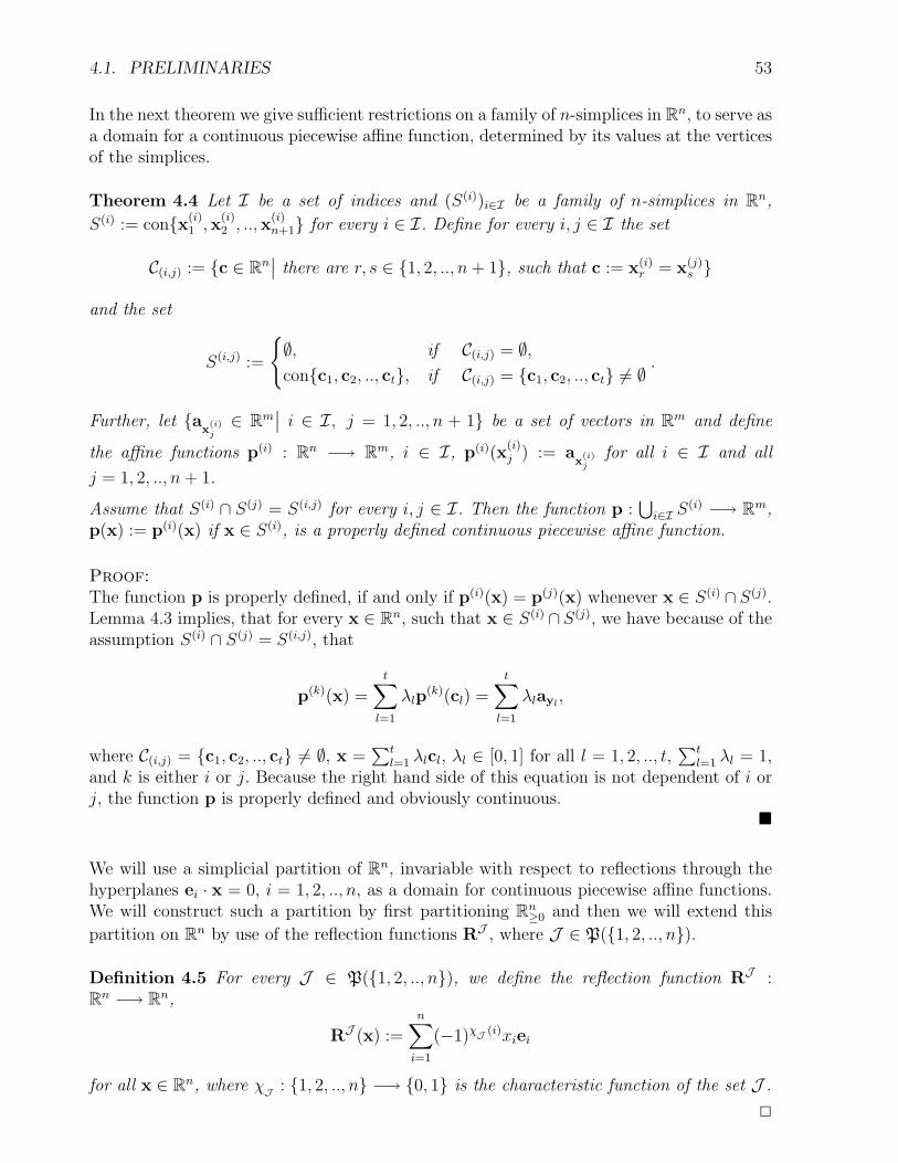
4.1. PRELIMINARIES 53
In the next theorem we give sufficient restrictions on a family of n-simplices in Rn, to serve asa domain for a continuous piecewise affine function, determined by its values at the verticesof the simplices.
Theorem 4.4 Let I be a set of indices and (S(i))i∈I be a family of n-simplices in Rn,
S(i) := con{x(i)1 ,x
(i)2 , ..,x
(i)n+1} for every i ∈ I. Define for every i, j ∈ I the set
C(i,j) := {c ∈ Rn∣∣ there are r, s ∈ {1, 2, .., n+ 1}, such that c := x(i)
r = x(j)s }
and the set
S(i,j) :=
{∅, if C(i,j) = ∅,con{c1, c2, .., ct}, if C(i,j) = {c1, c2, .., ct} 6= ∅
.
Further, let {ax
(i)j∈ Rm
∣∣ i ∈ I, j = 1, 2, .., n + 1} be a set of vectors in Rm and define
the affine functions p(i) : Rn −→ Rm, i ∈ I, p(i)(x(i)j ) := a
x(i)j
for all i ∈ I and all
j = 1, 2, .., n+ 1.
Assume that S(i) ∩ S(j) = S(i,j) for every i, j ∈ I. Then the function p :⋃
i∈I S(i) −→ Rm,
p(x) := p(i)(x) if x ∈ S(i), is a properly defined continuous piecewise affine function.
Proof:The function p is properly defined, if and only if p(i)(x) = p(j)(x) whenever x ∈ S(i) ∩ S(j).Lemma 4.3 implies, that for every x ∈ Rn, such that x ∈ S(i) ∩ S(j), we have because of theassumption S(i) ∩ S(j) = S(i,j), that
p(k)(x) =t∑
l=1
λlp(k)(cl) =
t∑l=1
λlayl,
where C(i,j) = {c1, c2, .., ct} 6= ∅, x =∑t
l=1 λlcl, λl ∈ [0, 1] for all l = 1, 2, .., t,∑t
l=1 λl = 1,and k is either i or j. Because the right hand side of this equation is not dependent of i orj, the function p is properly defined and obviously continuous.
�
We will use a simplicial partition of Rn, invariable with respect to reflections through thehyperplanes ei · x = 0, i = 1, 2, .., n, as a domain for continuous piecewise affine functions.We will construct such a partition by first partitioning Rn
≥0 and then we will extend this
partition on Rn by use of the reflection functions RJ , where J ∈ P({1, 2, .., n}).
Definition 4.5 For every J ∈ P({1, 2, .., n}), we define the reflection function RJ :Rn −→ Rn,
RJ (x) :=n∑
i=1
(−1)χJ (i)xiei
for all x ∈ Rn, where χJ : {1, 2, .., n} −→ {0, 1} is the characteristic function of the set J .
2

54 CHAPTER 4. CONTINUOUS PIECEWISE AFFINE FUNCTIONS
Clearly RJ , where J = {j1, j2, .., jk}, represents reflections through the hyperplanes ej1 ·x =0, ej2 · x = 0, .., and ejk
· x = 0 in succession.
Let (S(i))i∈I be a family of n-simplices in Rn fulfilling the assumptions of Theorem 4.4,such that every simplex S(i), i ∈ I, is entirely contained in Rn
≥0. Then for every J ∈P({1, 2, .., n}), the family (RJ (S(i)))i∈I is entirely contained in
{x ∈ Rn∣∣ xi ∈ ]−∞, 0] if i ∈ J and xi ∈ [0,+∞[ otherwise}
and trivially, because RJ is linear and one-to-one, fulfills the assumptions of Theorem 4.4.In the next theorem we will show that even the family (RJ (S(i)))i∈I,J∈P({1,2,..,n}) fulfills theassumptions of Theorem 4.4.
Theorem 4.6 Let I be a set of indices and (S(i))i∈I be a family of n-simplices contained inRn≥0, fulfilling the assumptions of Theorem 4.4. Then the family (RJ (S(i)))i∈I,J∈P({1,2,..,n})
fulfills the assumptions of Theorem 4.4 too.
Proof:Let J ∈ P({1, 2, .., n}) and i, j ∈ I be arbitrary. Then clearly S(i) ∩ S(j) = ∅ impliesRJ (S(i)) ∩ S(j) = ∅. Assume that S(i) ∩ S(j) 6= ∅, then the simplices S(i) and S(j) havecommon vertices, c1, c2, .., ck, such that S(i) ∩ S(j) = con{c1, c2, .., ck}. Define the set
C ′ = {c′1, c′2, .., c′r} := {c′ ∈ {c1, c2, .., ck}∣∣ RJ (c′) = c′}.
One easily sees that if C ′ = ∅, then RJ (S(i))∩S(j) = ∅ and if C ′ 6= ∅, then RJ (S(i))∩S(j) =con{c′1, c′2, .., c′r}. Now let J1,J2 ∈ P({1, 2, .., n}) and i, j ∈ I be arbitrary. Because RJ2 isone-to-one and its own inverse, we have
RJ1(S(i)) ∩RJ2(S(j)) = RJ2(RJ2 [RJ1(S(i)) ∩RJ2(S(j))])
= RJ2(RJ2 [RJ1(S(i))] ∩RJ2 [RJ2(S(j))])
= RJ2(RJ1∆J2(S(i))] ∩ S(j)),
where J1∆J2 := (J1 ∪ J2) \ (J1 ∩ J2) is the set theoretic symmetric difference. Becauseof the previous considerations and because RJ2 is a one-to-one linear mapping, the setRJ1(S(i)) ∩ RJ2(S(j)) is either empty or a simplex, determined by the vertices that arecommon to RJ1(S(i)) and RJ2(S(j)). This means, that the family (RJ (S(i)))i∈I,J∈P({1,2,..,n})fulfills the assumptions of Theorem 4.4.
�
4.2 Simplicial Partition of Rn
From Theorem 4.4 we know what properties of a family of n-simplices in Rn are sufficient,for them to serve as a domain for a continuous piecewise affine function. In this section wewill give a concrete simplicial partition of Rn, where the simplices of the partition fulfill theassumptions of Theorem 4.4.
For every n ∈ Z>0, we denote by Symn the permutation group of {1, 2, .., n}, i.e. Symn isthe set of the one-to-one mappings from {1, 2, .., n} onto itself.
The simplices Sσ, where σ ∈ Symn , serve as the atoms of our partition. They are definedin the following way.
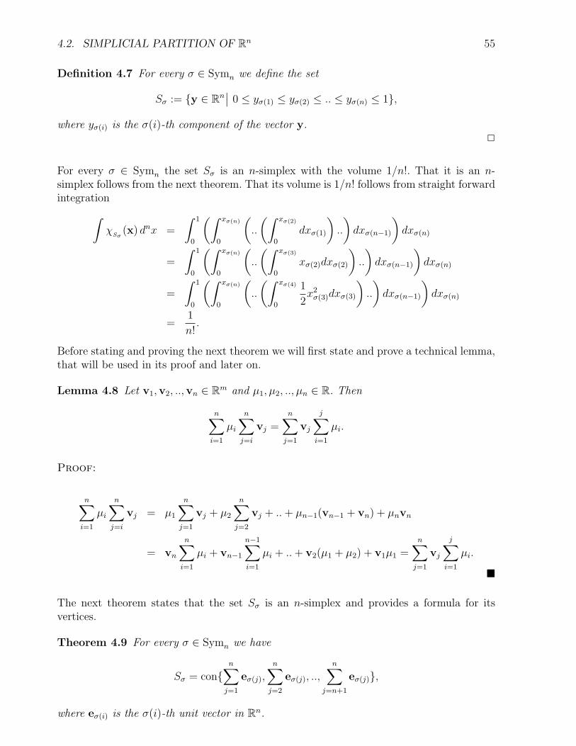
4.2. SIMPLICIAL PARTITION OF Rn 55
Definition 4.7 For every σ ∈ Symn we define the set
Sσ := {y ∈ Rn∣∣ 0 ≤ yσ(1) ≤ yσ(2) ≤ .. ≤ yσ(n) ≤ 1},
where yσ(i) is the σ(i)-th component of the vector y.2
For every σ ∈ Symn the set Sσ is an n-simplex with the volume 1/n!. That it is an n-simplex follows from the next theorem. That its volume is 1/n! follows from straight forwardintegration∫
χSσ
(x) dnx =
∫ 1
0
(∫ xσ(n)
0
(..
(∫ xσ(2)
0
dxσ(1)
)..
)dxσ(n−1)
)dxσ(n)
=
∫ 1
0
(∫ xσ(n)
0
(..
(∫ xσ(3)
0
xσ(2)dxσ(2)
)..
)dxσ(n−1)
)dxσ(n)
=
∫ 1
0
(∫ xσ(n)
0
(..
(∫ xσ(4)
0
1
2x2
σ(3)dxσ(3)
)..
)dxσ(n−1)
)dxσ(n)
=1
n!.
Before stating and proving the next theorem we will first state and prove a technical lemma,that will be used in its proof and later on.
Lemma 4.8 Let v1,v2, ..,vn ∈ Rm and µ1, µ2, .., µn ∈ R. Then
n∑i=1
µi
n∑j=i
vj =n∑
j=1
vj
j∑i=1
µi.
Proof:
n∑i=1
µi
n∑j=i
vj = µ1
n∑j=1
vj + µ2
n∑j=2
vj + ..+ µn−1(vn−1 + vn) + µnvn
= vn
n∑i=1
µi + vn−1
n−1∑i=1
µi + ..+ v2(µ1 + µ2) + v1µ1 =n∑
j=1
vj
j∑i=1
µi.
�
The next theorem states that the set Sσ is an n-simplex and provides a formula for itsvertices.
Theorem 4.9 For every σ ∈ Symn we have
Sσ = con{n∑
j=1
eσ(j),
n∑j=2
eσ(j), ..,
n∑j=n+1
eσ(j)},
where eσ(i) is the σ(i)-th unit vector in Rn.

56 CHAPTER 4. CONTINUOUS PIECEWISE AFFINE FUNCTIONS
Proof:We first show, that
con{n∑
j=1
eσ(j),n∑
j=2
eσ(j), ..,n∑
j=n+1
eσ(j)} ⊆ Sσ.
Let
y ∈ con{n∑
j=1
eσ(j),
n∑j=2
eσ(j), ..,
n∑j=n+1
eσ(j)}.
Then there are λ1, λ2, .., λn+1 ∈ [0, 1], such that
y =n+1∑i=1
λi
n∑j=i
eσ(j) andn+1∑i=1
λi = 1.
Because
yσ(k) = y · eσ(k) =
(n+1∑i=1
λi
n∑j=i
eσ(j)
)· eσ(k) =
n+1∑i=1
n∑j=i
λiδjk =k∑
i=1
λi,
it follows that yσ(k) ∈ [0, 1] and yσ(k) ≤ yσ(l) if k ≤ l, so y ∈ Sσ.
We now show that
Sσ ⊆ con{n∑
j=1
eσ(j),n∑
j=2
eσ(j), ..,n∑
j=n+1
eσ(j)}.
Let y ∈ Sσ. Then 0 ≤ yσ(1) ≤ yσ(2) ≤ .. ≤ yσ(n) ≤ 1. Set
λ1 := yσ(1),
λ2 := yσ(2) − yσ(1),
λ3 := yσ(3) − yσ(2),
:
λn := yσ(n) − yσ(n−1),
and
λn+1 = 1− yσ(n).
Then obviouslyn+1∑i=1
λi = 1
and by Lemma 4.8
y =n∑
j=1
j∑i=1
λieσ(j) =n+1∑i=1
λi
n∑j=i
eσ(j),
i.e.
y ∈ con{n∑
j=1
eσ(j),
n∑j=2
eσ(j), ..,
n∑j=n+1
eσ(j)}.
�

4.2. SIMPLICIAL PARTITION OF Rn 57
In the next two theorems we will show, that the family of simplices (z + Sσ)z∈Zn≥0,σ∈Symn
partitions Rn≥0 and is compatible with the assumptions of Theorem 4.4. We start by showing
that the simplices (Sσ)σ∈Symnpartition the set [0, 1]n in the appropriate way.
Theorem 4.10 Let α, β ∈ Symn. Then
Sα ∩ Sβ = con{c1, c2, .., ck},
where the c1, c2, .., ck are the vertices that are common to Sα and Sβ, i.e.
{c1, c2, .., ck} := {x ∈ Rn∣∣x =
n∑j=a
eα(j) =n∑
j=a
eβ(j) for some a ∈ {1, 2, .., n+ 1}}.
Proof:The inclusion
Sα ∩ Sβ ⊃ con{c1, c2, .., ck}is trivial, so we only have to prove
Sα ∩ Sβ ⊂ con{c1, c2, .., ck}. (4.2)
To do this define σ ∈ Symn, σ := β−1α, and the set
Aσ := {x ∈ {1, 2, .., n+ 1}∣∣σ({1, 2, .., x− 1}) = {1, 2, .., x− 1}}.
Clearly
Aσ := {x ∈ {1, 2, .., n+ 1}∣∣σ({1, 2, .., x− 1}) = {1, 2, .., x− 1}}
= {x ∈ {1, 2, .., n+ 1}∣∣σ({x, x+ 1, .., n}) = {x, x+ 1, .., n}}
= {x ∈ {1, 2, .., n+ 1}∣∣β−1α({x, x+ 1, .., n}) = {x, x+ 1, .., n}}
= {x ∈ {1, 2, .., n+ 1}∣∣α({x, x+ 1, .., n}) = β({x, x+ 1, .., n})}
andn∑
j=a
eα(j) =n∑
j=b
eβ(j),
if and only if a = b and α({a, a+ 1, .., n}) = β({b, b+ 1, .., n}).Hence
{c1, c2, .., ck} = {n∑
j=a1
eα(j),n∑
j=a2
eα(j), ..,n∑
j=ak
eα(j)},
where the a1, a2, .., ak are the elements of Aσ. For convenience let a1 < a2 < .. < ak.
Let x be an arbitrary element in Sα ∩Sβ. Then there are µi, λi ∈ [0, 1], for i = 1, 2, .., n+ 1,such that
n+1∑i=1
µi =n+1∑i=1
λi = 1
and
x =n+1∑i=1
µi
n∑j=i
eα(j) =n+1∑i=1
λi
n∑j=i
eβ(j).

58 CHAPTER 4. CONTINUOUS PIECEWISE AFFINE FUNCTIONS
We prove (4.2) by showing by mathematical induction, that µi = λi for all i ∈ {1, 2, .., n+1}and that µi = λi = 0 for all i ∈ {1, 2, .., n+ 1} \ Aσ.
Lemma 4.8 implies
x =n∑
j=1
eα(j)
j∑i=1
µi =n∑
j=1
eβ(j)
j∑i=1
λi.
By comparing the components of the vectors on the left-hand and the right-hand side ofthis equation, we see that for every pair (r, s) ∈ {1, 2, .., n}2, such that α(r) = β(s), we musthave
r∑i=1
µi =s∑
i=1
λi,
i.e.m∑
i=1
µi =
σ(m)∑i=1
λi andm∑
i=1
λi =
σ−1(m)∑i=1
µi (4.3)
for all m = 1, 2, .., n.
Let P (r) be the proposition: ”µi = λi for all i ∈ {1, 2, .., ar − 1} and µi = λi = 0 for alli ∈ {1, 2, .., ar − 1} \ {a1, a2, .., ar−1}”From the definition of Aσ it follows that a1 = 1, so the proposition P (1) is obviously true.There is indeed nothing to prove. We show that for r < k, P (r) implies P (r + 1).
Assume that P (r) is true for some 1 ≤ r < k. Then µi = λi for all i = 1, 2, .., ar−1 and σ(ar)and σ−1(ar) must be greater than or equal to ar. If σ(ar) = σ−1(ar) = ar, then triviallyar + 1 ∈ Aσ, i.e. ar+1 = ar + 1, and it follows from (4.3) that µar = λar , which implies thatP (r + 1) is true.
Suppose σ(ar) and σ−1(ar) are greater that ar. Then it follows from (4.3), that
ar∑i=1
µi =
σ(ar)∑i=1
λi =ar−1∑i=1
µi + λar +
σ(ar)∑i=ar+1
λi,
i.e.
µar = λar +
σ(ar)∑i=ar+1
λi,
and similarly
λar = µar +
σ−1(ar)∑i=ar+1
µi.
By adding the two last equation, we see that
σ(ar)∑i=ar+1
λi +
σ−1(ar)∑i=ar+1
µi = 0
and because µi, λi ∈ [0, 1] for all i = 1, 2, .., n, this implies that
µar+1 = µar+2 = .. = µσ−1(ar) = 0,

4.2. SIMPLICIAL PARTITION OF Rn 59
λar+1 = λar+2 = .. = λσ(ar) = 0,
andµar = λar .
Define the integers a and b by
a := max{s < ar+1
∣∣µar+1 = µar+2 = .. = µs = 0}
andb := max{s < ar+1
∣∣λar+1 = λar+2 = .. = λs = 0}.For all m ∈ {ar + 1, ar + 2, .., a} we have
σ(m)∑i=1
λi =m∑
i=1
µi =ar∑i=1
µi
and because µi = λi for all i = 1, 2, .., ar, this implies that
σ(m)∑i=ar+1
λi = 0,
i.e. thatλar+1 = λar+2 = .. = λσ(m) = 0.
Therefore
b ≥ max{σ(m)∣∣m = ar + 1, ar + 2, .., a} = max{σ(m)
∣∣m = 1, 2, .., a},
where the equality on the right-hand side is a consequence of σ({1, 2, .., ar − 1}) ={1, 2, .., ar − 1} and b ≥ σ(ar).
The set {σ(m)∣∣m = 1, 2, .., a} is a subset of {1, 2, .., n} with a distinct elements, so
max{σ(m)∣∣m = 1, 2, .., a} ≥ a,
i.e. b ≥ a. With similar reasoning, we can show that a ≥ b. Hence a = b.
We have shown that µar = λar , that there is a constant a, with ar < a < ar+1, such that
µar+1 = µar+2 = .. = µa = λar+1 = λar+2 = .. = λa = 0,
and that σ({1, 2, .., a}) = {1, 2, .., a}. This implies a+1 = ar+1 ∈ Aσ and that the propositionP (r + 1) is true, which completes the mathematical induction.
�
We now apply the last theorem to prove that (s + Sσ)s∈Zn≥0, σ∈Symn
partitions Rn≥0 in the
appropriate way.
Theorem 4.11 Let α, β ∈ Symn and sα, sβ ∈ Zn. Let C = {c1, c2, .., ck} be the set of thevertices common to the simplices sα + Sα and sβ + Sβ. Then (sα + Sα) ∩ (sβ + Sβ) = ∅ ifC = ∅ and
(sα + Sα) ∩ (sβ + Sβ) = con{c1, c2, .., ck}if C 6= ∅.
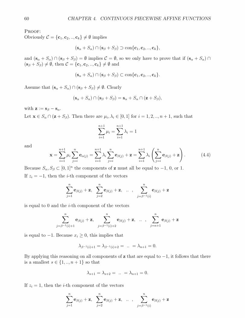
60 CHAPTER 4. CONTINUOUS PIECEWISE AFFINE FUNCTIONS
Proof:Obviously C = {c1, c2, .., ck} 6= ∅ implies
(sα + Sα) ∩ (sβ + Sβ) ⊃ con{c1, c2, .., ck},
and (sα + Sα) ∩ (sβ + Sβ) = ∅ implies C = ∅, so we only have to prove that if (sα + Sα) ∩(sβ + Sβ) 6= ∅, then C = {c1, c2, .., ck} 6= ∅ and
(sα + Sα) ∩ (sβ + Sβ) ⊂ con{c1, c2, .., ck}.
Assume that (sα + Sα) ∩ (sβ + Sβ) 6= ∅. Clearly
(sα + Sα) ∩ (sβ + Sβ) = sα + Sα ∩ (z + Sβ),
with z := sβ − sα.
Let x ∈ Sα ∩ (z + Sβ). Then there are µi, λi ∈ [0, 1] for i = 1, 2, .., n+ 1, such that
n+1∑i=1
µi =n+1∑i=1
λi = 1
and
x =n+1∑i=1
µi
n∑j=i
eα(j) =n+1∑i=1
λi
n∑j=i
eβ(j) + z =n+1∑i=1
λi
(n∑
j=i
eβ(j) + z
). (4.4)
Because Sα, Sβ ⊂ [0, 1]n the components of z must all be equal to −1, 0, or 1.
If zi = −1, then the i-th component of the vectors
n∑j=1
eβ(j) + z,n∑
j=2
eβ(j) + z, .. ,n∑
j=β−1(i)
eβ(j) + z
is equal to 0 and the i-th component of the vectors
n∑j=β−1(i)+1
eβ(j) + z,n∑
j=β−1(i)+2
eβ(j) + z, .. ,
n∑j=n+1
eβ(j) + z
is equal to −1. Because xi ≥ 0, this implies that
λβ−1(i)+1 = λβ−1(i)+2 = .. = λn+1 = 0.
By applying this reasoning on all components of z that are equal to −1, it follows that thereis a smallest s ∈ {1, .., n+ 1} so that
λs+1 = λs+2 = .. = λn+1 = 0.
If zi = 1, then the i-th component of the vectors
n∑j=1
eβ(j) + z,n∑
j=2
eβ(j) + z, .. ,
n∑j=β−1(i)
eβ(j) + z

4.2. SIMPLICIAL PARTITION OF Rn 61
is equal to 2 and the i-th component of the vectors
n∑j=β−1(i)+1
eβ(j) + z,n∑
j=β−1(i)+2
eβ(j) + z, .. ,
n∑j=n+1
eβ(j) + z
is equal to 1. Because xi ≤ 1, this implies that
λ1 = λ2 = .. = λβ−1(i) = 0.
By applying this reasoning on all components of z that are equal to 1, it follows that thereis a largest r ∈ {1, 2, .., n+ 1} so that
λ1 = λ2 = .. = λr−1 = 0.
If r > s then λ1 = λ2 = .. = λn+1 = 0, which is in contradiction to their sum being equal to1. Therefore r ≤ s.
From the definitions of r and s it follows, that the components of the vectors
n∑j=r
eβ(j) + z,n∑
j=r+1
eβ(j) + z, .. ,n∑
j=s
eβ(j) + z
are all equal to 0 or 1. Let a1, a2, .., at−1 be the indices of those components of
n∑j=r
eβ(j) + z
that are equal to 0. By defining the permutation γ ∈ Symn as follows,
γ(i) := ai, for all i = 1, 2, .., t− 1,
γ(i) := β(r + i− t), for all i = t, t+ 1, .., t+ s− r,
and with {bt+s−r+1, bt+s−r+2, .., bn} := {1, 2, .., n} \ γ({1, 2, .., t+ s− r}),
γ(i) := bi, for all i = t+ s− r + 1, t+ s− r + 2, .., n,
we obtain,n∑
i=t+j
eγ(i) =n∑
i=r+j
eβ(i) + z. (4.5)
for all j = 0, 1, .., s− r. To see this, note that
n∑i=t
eγ(i)
has all components equal to 1, except for those with an index from the set γ({1, 2, .., t−1}),which are equal to 0. But from γ({1, 2, .., t− 1}) = {a1, a2, .., at−1} and the definition of theindices ai, it follows that
n∑i=t
eγ(i) =n∑
i=r
eβ(i) + z.
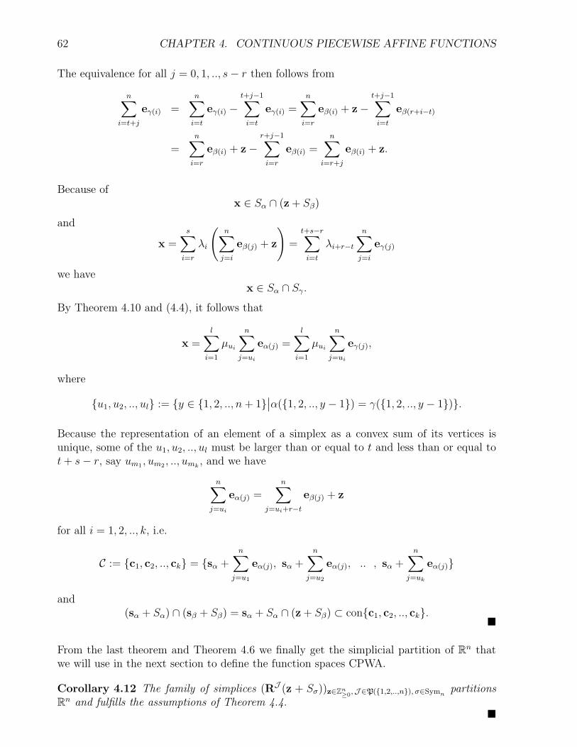
62 CHAPTER 4. CONTINUOUS PIECEWISE AFFINE FUNCTIONS
The equivalence for all j = 0, 1, .., s− r then follows from
n∑i=t+j
eγ(i) =n∑
i=t
eγ(i) −t+j−1∑
i=t
eγ(i) =n∑
i=r
eβ(i) + z−t+j−1∑
i=t
eβ(r+i−t)
=n∑
i=r
eβ(i) + z−r+j−1∑
i=r
eβ(i) =n∑
i=r+j
eβ(i) + z.
Because ofx ∈ Sα ∩ (z + Sβ)
and
x =s∑
i=r
λi
(n∑
j=i
eβ(j) + z
)=
t+s−r∑i=t
λi+r−t
n∑j=i
eγ(j)
we havex ∈ Sα ∩ Sγ.
By Theorem 4.10 and (4.4), it follows that
x =l∑
i=1
µui
n∑j=ui
eα(j) =l∑
i=1
µui
n∑j=ui
eγ(j),
where
{u1, u2, .., ul} := {y ∈ {1, 2, .., n+ 1}∣∣α({1, 2, .., y − 1}) = γ({1, 2, .., y − 1})}.
Because the representation of an element of a simplex as a convex sum of its vertices isunique, some of the u1, u2, .., ul must be larger than or equal to t and less than or equal tot+ s− r, say um1 , um2 , .., umk
, and we have
n∑j=ui
eα(j) =n∑
j=ui+r−t
eβ(j) + z
for all i = 1, 2, .., k, i.e.
C := {c1, c2, .., ck} = {sα +n∑
j=u1
eα(j), sα +n∑
j=u2
eα(j), .. , sα +n∑
j=uk
eα(j)}
and(sα + Sα) ∩ (sβ + Sβ) = sα + Sα ∩ (z + Sβ) ⊂ con{c1, c2, .., ck}.
�
From the last theorem and Theorem 4.6 we finally get the simplicial partition of Rn thatwe will use in the next section to define the function spaces CPWA.
Corollary 4.12 The family of simplices (RJ (z + Sσ))z∈Zn≥0,J∈P({1,2,..,n}), σ∈Symn
partitionsRn and fulfills the assumptions of Theorem 4.4.
�

4.3. THE FUNCTION SPACES CPWA 63
4.3 The Function Spaces CPWA
In this section we will introduce the function spaces CPWA and derive some results regardingthe functions in these spaces, that will be useful when we prove that a feasible solution of alinear program generated by Linear Program LP2 can be used to define a CPWA Lyapunovfunction.
A CPWA space is a set of continuous affine functions from a subset of Rn into R with a givenboundary configuration. If the subset is compact, then the boundary configuration makes itpossible to parameterize the functions in the respective CPWA space with a finite numberof real parameters. Further, the CPWA spaces are vector spaces over R in the canonicalway. They are thus well suited as a foundation, in the search of a Lyapunov function witha linear program.
We first define the function spaces CPWA for subsets of Rn that are the unions of n-dimensional cubes.
Definition 4.13 Let Z ⊂ Zn, Z 6= ∅, be such that the set
N :=⋃z∈Z
(z + [0, 1]n),
is connected.
The function space CPWA[N ] is then defined as follows.
The function p : N −→ R is in CPWA[N ], if and only if:
i) p is continuous.
ii) For every simplex RJ (z+Sσ), z ∈ Zn≥0, J ∈ P({1, 2, .., n}), and σ ∈ Symn, contained
in N , the restriction p|RJ (z+Sσ) is affine.2
It follows from Corollary 4.12 that the set CPWA[N ] is not empty and that its elements areuniquely determined by their values on the set N ∩ Zn.
We will need continuous piecewise affine functions, defined by their values on grids withsmaller grid steps than one, and we want to use grids with variable grid steps. We achievethis by using images of Zn under mappings Rn −→ Rn, of which the components arecontinuous and strictly increasing functions on R −→ R, affine on the intervals [m,m + 1]where m is an integer, and map zero on itself. We call such Rn −→ Rn mappings piecewisescaling functions.
Definition 4.14 A function PS : Rn −→ Rn is called a piecewise scaling function, if andonly if PS(0) = 0 and
PS(x) = (PS1(x),PS2(x), ..,PSn(x)) = (PS1(x1), PS2(x2), .., PSn(xn))
for all x ∈ Rn, where PSi ∈ CPWA[R] and is strictly increasing on R for all i = 1, 2, .., n.2

64 CHAPTER 4. CONTINUOUS PIECEWISE AFFINE FUNCTIONS
Note that if yi,j, i = 1, 2, .., n and j ∈ Z, are real numbers such that yi,j < yi,j+1 andyi,0 = 0 for all i = 1, 2, .., n and all j ∈ Z, then we can define a piecewise scaling function
PS : Rn −→ Rn, by PSi(j) := yi,j for all i = 1, 2, .., n and all j ∈ Z. Moreover, the piecewisescaling functions Rn −→ Rn are exactly the functions, that can be constructed in this way.
In the next definition we use piecewise scaling functions to define general CPWA spaces.
Definition 4.15 Let PS : Rn −→ Rn be a piecewise scaling function and let Z ⊂ Zn,Z 6= ∅, be such that the set
N :=⋃z∈Z
(z + [0, 1]n)
is connected.
The function space CPWA[PS,N ] is defined as
CPWA[PS,N ] := {p ◦PS−1∣∣ p ∈ CPWA[N ]}
and we denote by S[PS,N ] the set of the simplices in the family
(PS(RJ (z + Sσ)))z∈Zn≥0, J∈P({1,2,..,n}), σ∈Symn
that are contained in the image PS(N ) of N under PS.2
Clearly{x ∈ Rn
∣∣ x is a vertex of a simplex in S[PS,N )]} = PS(N ∩ Zn)
and every function in CPWA[PS,N ] is uniquely determined by its values on the grid PS(N∩Zn).
We will use functions from CPWA[PS,N ] to approximate functions in C(PS(N )), whichhave bounded second order derivatives on the interiors of the simplices in S[PS,N ] . Thenext lemma gives upper bounds of the approximation error of such an approximation.
Lemma 4.16 Let con{x1,x2..,xn+1} be an n-simplex in Rn and g : con{x1,x2..,xn+1} −→R be a function, such that the partial derivatives
∂2g
∂xl∂xk
exist in the interior of con{x1,x2..,xn+1} for all k, l = 1, 2, .., n. Further, assume that theyare continuous and bounded, i.e. there are constants Bkl < +∞, k, l = 1, 2, .., n, such that∣∣∣∣ ∂2g
∂xl∂xk
(x)
∣∣∣∣ ≤ Bkl
for all x in the interior of con{x1,x2..,xn+1} and all k, l = 1, 2, .., n.
Let a : con{x1,x2..,xn+1} −→ R be an affine function, defined by
a(xi) = g(xi), for all i = 1, 2, .., n+ 1.
Then for any x =∑n+1
i=1 λixi, 0 ≤ λi ≤ 1 for all i = 1, 2, .., n+ 1, and∑n+1
i=1 λi = 1, we havefor any d ∈ {1, 2, .., n+ 1}, that
|g(x)− a(x)| ≤ 1
2
n+1∑i=1
λi
n∑k,l=1
Bkl|ek · (xi − xd)|(|el · (x− xd)|+ |el · (xi − xd)|).

4.3. THE FUNCTION SPACES CPWA 65
Proof:Because simplices are convex sets, there is an y ∈ Rn and for every x ∈ con{x1,x2..,xn+1}an yx ∈ Rn, such that r(xd + sy) + (1− r)(x + syx) is in the interior of con{x1,x2..,xn+1}for all r ∈ [0, 1] and all s ∈ ]0, 1]. It follows from Taylor’s theorem that for every x ∈con{x1,x2..,xn+1} and every s ∈ ]0, 1] there is a zs,x ∈ con{x1,x2..,xn+1}, such that
g(x + syx) = g(xd + sy) +∇g(xd + sy) · (x− xd + s(yx − y))
+1
2
n∑k,l=1
[ek · (x− xd + s(yx − y))][el · (x− xd + s(yx − y))]∂2g
∂xk∂xl
(zs,x).
Because the second order derivatives of g are bounded on the interior of con{x1,x2..,xn+1},we can extend ∇g to a continuous function on con{x1,x2..,xn+1}, let s→ 0+, and get
g(x) = g(xd) +∇g(xd) · (x− xd) +1
2
n∑k,l=1
[ek · (x− xd)][el · (x− xd)]bkl,x,
where bkl,x ∈ [−Bkl, Bkl] for all k, l = 1, 2, .., n. Set
ex :=1
2
n∑k,l=1
[ek · (x− xd)][el · (x− xd)]bkl,x.
Let x ∈ con{x1,x2..,xn+1} be arbitrary. Then there are real numbers λ1, λ2, .., λn+1 ∈ [0, 1]such that
x =n+1∑i=1
λixi andn+1∑i=1
λi = 1,
and we get from Lemma 4.3 and by repeated use of Taylor’s theorem
g(x)− a(x) = g(xd) +∇g(xd) · (x− xd) + ex −n+1∑i=1
λig(xi)
= ex +n+1∑i=1
λi [∇g(xd) · (xi − xd)− (g(xi)− g(xd))]
= ex +n+1∑i=1
λi[∇g(xd) · (xi − xd)− (g(xd) +∇g(xd) · (xi − xd) + exi− g(xd))]
= ex −n+1∑i=1
λiexi
=1
2
n+1∑i=1
λi
n∑k,l=1
([ek · (xi − xd)][el · (x− xd)]bkl,x − [ek · (xi − xd)][el · (xi − xd)]bkl,xi) ,
from which
|g(x)− a(x)| ≤ 1
2
n+1∑i=1
λi
n∑k,l=1
Bkl|ek · (xi − xd)|(|el · (x− xd)|+ |el · (xi − xd)|)
follows.

66 CHAPTER 4. CONTINUOUS PIECEWISE AFFINE FUNCTIONS
�
Linear Program LP2 tries to parameterize a CPWA Lyapunov function for a system. Be-cause a CPWA Lyapunov function is not differentiable, one can not use the chain rule toget
d
dtV (φ(t, ξ))
∣∣∣∣t=0
= ∇V (ξ) · f(ξ),
where φ is the solution of x = f(x), which makes it possible to use Lyapunov’s directmethod without integrating the system equation. The next theorem gives a substitute forthis equation when V ∈ CPWA.
Theorem 4.17 Let PS : Rn −→ Rn be a piecewise scaling function, N ⊂ Rn be such thatthe space CPWA[PS,N ] is properly defined, and let V ∈ CPWA[PS,N ]. Define H ⊂ Rn
as the interior of the set PS(N ) and let U ⊂ Rn be a domain, H ⊂ U , and f : U −→ Rn bea locally Lipschitz function. Denote by φ the solution of the system
x = f(x).
Further, let D∗ ∈ {D+, D+, D−, D−} be a Dini derivative with respect to t.
For every S(i) ∈ S[PS,N ] let w(i) ∈ Rn and ai ∈ R be such that V (x) = w(i) · x + ai for allx ∈ S(i).
Assume there is a function γ : Rn −→ R, such that for every S(i) ∈ S[PS,N ], we have forevery x ∈ S(i) ∩H, that
w(i) · f(x) ≤ γ(x).
Then
D∗[V (φ(t, ξ))] ≤ γ(φ(t, ξ))
whenever φ(t, ξ) ∈ H.
Proof:We only prove the theorem for D∗ = D+, the cases D∗ = D+, D∗ = D−, and D∗ = D−follow analogously. Let φ(t, ξ) ∈ H be arbitrary. Then there is a simplex S(i) ∈ S[PS,N ]and a δ > 0, such that φ(t, ξ) + sf(φ(t, ξ)) ∈ S(i) for all s ∈ [0, δ] (simplices are convexsets).
It follows from Theorem 1.17, that
D+[V (φ(t, ξ))] = lim sups→0+
V (φ(t, ξ) + sf(φ(t, ξ)))− V (φ(t, ξ))
s
= lim sups→0+
w(i) · [φ(t, ξ) + sf(φ(t, ξ))] + ai −w(i) · φ(t, ξ)− ai
s
= lim sups→0+
sw(i) · f(φ(t, ξ))
s= w(i) · f(φ(t, ξ)) ≤ γ(φ(t, ξ)).
�
The next lemma gives a formula for the gradient of a piecewise affine function, in its valuesat the vertices of the simplex PS(RJ (z + Sσ)).
4.3. THE FUNCTION SPACES CPWA 67
Lemma 4.18 Let PS : Rn −→ Rn be a piecewise scaling function, z ∈ Zn≥0, J ∈
P({1, 2, .., n}), and σ ∈ Symn. Then the simplex PS(RJ (z + Sσ)) has the vertices PS(x1),PS(x2), ..,PS(xn+1), where
xi := RJ (z +n∑
j=i
eσ(j)),
for i = 1, 2, .., n.
Let V : Rn −→ R,V (x) = w · x + a
for all x ∈ Rn, be an affine function. Then
w =n∑
i=1
V (PS(xi))− V (PS(xi+1))
PSσ(i)(xi)− PSσ(i)(xi+1)eσ(i) =
n∑i=1
(−1)χJ (σ(i))V (PS(xi))− V (PS(xi+1))
‖PS(xi)−PS(xi+1)‖∞eσ(i),
where χJ : {1, 2, .., n} −→ {0, 1} is the characteristic function of the set J .
Proof:We show that
wσ(i) =V (PS(xi))− V (PS(xi+1))
PSσ(i)(xi)− PSσ(i)(xi+1)
and thatPSσ(i)(xi)− PSσ(i)(xi+1) = (−1)χJ (σ(i))‖PS(xi)−PS(xi+1)‖∞
for all i = 1, 2, .., n.
For any i ∈ {1, 2, .., n} we have
V (PS(xi))− V (PS(xi+1)) = w · [PS(xi)−PS(xi+1)] =n∑
k=1
wσ(k)[PSσ(k)(xi)− PSσ(k)(xi+1)].
Because the components of the vectors
xi = RJ (z +n∑
j=i
eσ(j)) and xi+1 = RJ (z +n∑
j=i+1
eσ(j))
are all equal, except for the σ(i)-th one, it follows from the definition of a piecewise scalingfunction, that
PSσ(i)(xi)− PSσ(i)(xi+1) = (−1)χJ (σ(i))‖PS(xi)−PS(xi+1)‖∞
andV (PS(xi))− V (PS(xi+1)) = wσ(i)[PSσ(i)(xi)− PSσ(i)(xi+1)],
i.e.
wσ(i) =V (PS(xi))− V (PS(xi+1))
PSσ(i)(xi)− PSσ(i)(xi+1)= (−1)χJ (σ(i))V (PS(xi))− V (PS(xi+1))
‖PS(xi)−PS(xi+1)‖∞.
�
In this chapter we have defined the function spaces CPWA and we have proved severalproperties of the functions in these spaces. In the next chapter we will state Linear ProgramLP2 and we will use the results from this chapter to prove, that a CPWA Lyapunov functioncan be constructed from a feasible solution of a linear program generated by Linear ProgramLP2.

68 CHAPTER 4. CONTINUOUS PIECEWISE AFFINE FUNCTIONS

Chapter 5
Linear Program LP2
At the beginning of this chapter we will state Linear Program LP2, an algorithmicdescription of how to generate a linear program for a nonlinear system. In Section 5.1 wewill define the functions ψ, γ, and V Lya as continuous affine interpolations of variables ofsuch a linear program. In the sections 5.2-5.5 we will successively derive implications thatthe constraints of the linear program have on the functions ψ, γ, and V Lya . In Section 5.6we will state and prove Theorem II, a theorem which states that V Lya is a Lyapunov or aLyapunov-like function for the system in question.
Linear Program LP2Let f : U −→ Rn be locally Lipschitz, where U ⊂ Rn is a domain containing zero andf(0) = 0. Let PS : Rn −→ Rn be a piecewise scaling function, N ⊂ U be a bounded domaincontaining zero, and define the set
M :=⋃z∈Zn
PS(z+[0,1]n)⊂N
PS(z + [0, 1]n)
and assume that it is connected.
Let ‖ · ‖ be an arbitrary norm on Rn and
D := PS(]d−1 , d+1 [×]d−2 , d
+2 [× ..×]d−n , d
+n [)
be a set, of which the closure is contained in the interior of M, and either D = ∅ or d−i ≤ −1and 1 ≤ d+
i for all i = 1, 2, .., n.
Finally, assume that for every z ∈ Zn, such that PS(z + [0, 1]n) ⊂M\D, the second orderderivatives
∂2f1
∂xk∂xl
,∂2f2
∂xk∂xl
, .. ,∂2fn
∂xk∂xl
are continuous and bounded on PS(z+]0, 1[n) for all k, l = 1, 2, .., n.
Then the linear program LP2(f ,N ,PS,D, ‖ · ‖) is constructed in the following way:
i) Define the setX ‖·‖ := {‖x‖
∣∣ x ∈ PS(Zn) ∩M}.
69

70 CHAPTER 5. LINEAR PROGRAM LP2
ii) Define for every σ ∈ Symn and every i = 1, 2, .., n+ 1, the vector
xσi :=
n∑j=i
eσ(j).
iii) Define the set
Z := {(z,J ) ∈ Zn≥0 ×P({1, 2, .., n})
∣∣PS(RJ (z + [0, 1]n)) ⊂M\D}.
iv) For every (z,J ) ∈ Z define for every σ ∈ Symn and every i = 1, 2, .., n+1, the vector
y(z,J )σ,i := PS(RJ (z + xσ
i )).
v) Define the set
Y := {{y(z,J )σ,k ,y
(z,J )σ,k+1}
∣∣(z,J ) ∈ Z and k ∈ {1, 2, .., n}}.
The set Y is the set of neighboring grid points in the grid PS(Zn) ∩ (M\D).
vi) For every (z,J ) ∈ Z and every k, l = 1, 2, .., n let B(z,J )kl be a constant, such that
B(z,J )kl ≥ max
i=1,2,..,nsup
x∈PS(RJ (z+]0,1[n))
∣∣∣∣ ∂2fi
∂xk∂xl
(x)
∣∣∣∣and B
(z,J )kl < +∞.
vii) For every (z,J ) ∈ Z, every k, i = 1, 2, .., n, and every σ ∈ Symn, define
A(z,J )σ,k,i := |ek · (y(z,J )
σ,i − y(z,J )σ,n+1)|.
viii) Define the constant
x∂M,min := min{‖x‖∣∣x ∈ PS(Zn) ∩ ∂M},
where ∂M is the boundary of the set M.
ix) Let ε > 0 and δ > 0 be arbitrary constants.
The variables of the linear program are:
Ψ[x], for all x ∈ X ‖·‖,
Γ[x], for all x ∈ X ‖·‖,
V [x], for all x ∈ PS(Zn) ∩ (M\D),
C[{x,y}], for all {x,y} ∈ Y .
The linear constraints of the linear program are:

71
LC1) Let x1, x2, .., xK be the elements of X ‖·‖ in an increasing order. Then
Ψ[x1] = Γ[x1] = 0,
εx2 ≤ Ψ[x2],
εx2 ≤ Γ[x2],
and for every i = 2, 3, .., K − 1:
Ψ[xi]−Ψ[xi−1]
xi − xi−1
≤ Ψ[xi+1]−Ψ[xi]
xi+1 − xi
andΓ[xi]− Γ[xi−1]
xi − xi−1
≤ Γ[xi+1]− Γ[xi]
xi+1 − xi
.
LC2) For every x ∈ PS(Zn) ∩ (M\D):
Ψ[‖x‖] ≤ V [x].
If D = ∅, then
V [0] = 0.
If D 6= ∅, then for every x ∈ PS(Zn) ∩ ∂D:
V [x] ≤ Ψ[x∂M,min]− δ.
LC3) For every {x,y} ∈ Y:
−C[{x,y}] · ‖x− y‖∞ ≤ V [x]− V [y] ≤ C[{x,y}] · ‖x− y‖∞.
LC4) For every (z,J ) ∈ Z, every σ ∈ Symn, and every i = 1, 2, .., n+ 1:
−Γ[‖y(z,J )σ,i ‖] ≥
n∑j=1
V [y(z,J )σ,j ]− V [y
(z,J )σ,j+1]
eσ(j) · (y(z,J )σ,j − y
(z,J )σ,j+1)
fσ(j)(y(z,J )σ,i )
+1
2
n∑r,s=1
B(z,J )rs A
(z,J )σ,r,i (A
(z,J )σ,s,i + A
(z,J )σ,s,1 )
n∑j=1
C[{y(z,J )σ,j ,y
(z,J )σ,j+1}].
The objective of the linear program is not needed.�
Note that the values of the constants ε > 0 and δ > 0 do not affect whether there is afeasible solution of the linear program or not. If there is a feasible solution for ε := ε′ > 0and δ := δ′ > 0, then there is a feasible solution for all ε := ε∗ > 0 and δ := δ∗ > 0. Justmultiply all variables with
max{ε∗
ε′,δ∗
δ′}.

72 CHAPTER 5. LINEAR PROGRAM LP2
Assume that the linear program LP2(f ,N ,PS,D, ‖ · ‖) has a feasible solution, for someparticular f ,N ,PS, D, and ‖ · ‖, that satisfy the assumptions of the linear program, andlet φ be the solution of the system
x = f(x).
In the next five sections we will show that if the functions ψ, γ, and V Lya are defined aspiecewise affine interpolations of the values of the variables Ψ, Γ, and V respectively, thenψ, γ ∈ K,
ψ(‖x‖) ≤ V Lya(x)
for all x ∈M, and
D∗[V Lya(φ(t, ξ))] ≤ −γ(‖φ(t, ξ)‖),
where D∗ is an arbitrary Dini derivative with respect to t, for all φ(t, ξ) in the interior ofM.
5.1 The Definition of ψ, γ, and V Lya
Let x1, x2, .., xK be the elements of X ‖·‖ in an increasing order. We define the piecewiseaffine functions ψ, γ : [x1,+∞[−→ R,
ψ(y) := Ψ[xi] +Ψ[xi+1]−Ψ[xi]
xi+1 − xi
(y − xi)
and
γ(y) := Γ[xi] +Γ[xi+1]− Γ[xi]
xi+1 − xi
(y − xi),
for all y ∈ [xi, xi+1] and all i = 1, 2, .., K − 1. The values of ψ and γ on ]xK ,+∞[ do notreally matter, but to have everything properly defined, we set
ψ(y) := Ψ[xK−1] +Ψ[xK ]−Ψ[xK−1]
xK − xK−1
(y − xK−1)
and
γ(y) := Γ[xK−1] +Γ[xK ]− Γ[xK−1]
xK − xK−1
(y − xK−1)
for all y > xK . Clearly the functions ψ and γ are continuous.
The function V Lya ∈ CPWA[PS,PS−1(M)] is defined by
V Lya(x) := V [x]
for all x ∈M∩PS(Zn).
In the next four sections we will successively show, the implications the linear constraintsLC1, LC2, LC3, and LC4 have on ψ, γ, and V Lya .
5.2. THE CONSTRAINTS LC1 73
5.2 The Constraints LC1
The constraints LC1 are
Ψ[x1] = Γ[x1] = 0,
εx2 ≤ Ψ[x2],
εx2 ≤ Γ[x2],
andΨ[xi]−Ψ[xi−1]
xi − xi−1
≤ Ψ[xi+1]−Ψ[xi]
xi+1 − xi
(5.1)
andΓ[xi]− Γ[xi−1]
xi − xi−1
≤ Γ[xi+1]− Γ[xi]
xi+1 − xi
for every i = 2, 3, .., K − 1, where ε > 0 is a constant and x1, x2, .., xK are the elements ofX ‖·‖ in an increasing order.
We are going to show that the constraints LC1 imply, that the functions ψ and γ are convexand strictly increasing on [0,+∞[. Because x1 = 0, ψ(x1) = Ψ[x1] = 0, and γ(x1) = Γ[x1] =0, this means that they are convex K functions. The constraints are the same for Ψ and Γ,so it suffices to show this for the function ψ.
From the definition of ψ, it is clear that it is continuous and that
ψ(x)− ψ(y)
x− y=
Ψ[xi+1]−Ψ[xi]
xi+1 − xi
(5.2)
for all x, y ∈ [xi, xi+1] and all i = 1, 2, .., K − 1. From x1 = 0, Ψ[x1] = 0, and εx2 ≤ Ψ[x2]we get
ε ≤ Ψ[x2]−Ψ[x1]
x2 − x1
.
But then we get from (5.1) and (5.2) that D+ψ is a positive and increasing function on[x1,+∞[ and it follows from Corollary 1.13, that ψ is a strictly increasing function.
The function ψ is convex, if and only if for every y ∈ ]x1,+∞[ there are constants ay, by ∈ R,such that
ayy + by = ψ(y) and ayx+ by ≤ ψ(x)
for all x ∈ [x1,+∞[ (see, for example, Section 17 in Chapter 11 in [51]). Let y ∈ ]x1,+∞[.Because the function D+ψ is increasing, it follows from Theorem 1.12, that for every x ∈[x1,+∞[, there is a cx,y ∈ R, such that
ψ(x) = ψ(y) + cx,y(x− y)
and cx,y ≤ D+ψ(y) if x < y and cx,y ≥ D+ψ(y) if x > y. This means that
ψ(x) = ψ(y) + cx,y(x− y) ≥ D+ψ(y)x+ ψ(y)−D+ψ(y)y
for all x ∈ [x1,+∞[. Because y was arbitrary, the function ψ is convex.
74 CHAPTER 5. LINEAR PROGRAM LP2
5.3 The Constraints LC2
The constraints LC2 areΨ[‖x‖] ≤ V [x] (5.3)
for every x ∈ PS(Zn) ∩ (M\D),V [0] = 0
if D = ∅, andV [x] ≤ Ψ[x∂M,min]− δ
for every x ∈ PS(Zn) ∩ ∂D if D 6= ∅.Define the constant
V Lya∂M,min := min
x∈∂MV Lya(x)
and if D 6= ∅ the constantV Lya
∂D,max := maxx∈∂D
V Lya(x).
We are going to show that the constraints LC2 imply, that
ψ(‖x‖) ≤ V Lya(x)
for all x ∈M \D, thatV Lya(0) = 0
if D = ∅, and thatV Lya
∂D,max ≤ V Lya∂M,min − δ
if D 6= ∅.We first show that (5.3) implies, that
ψ(‖x‖) ≤ V Lya(x)
for all x ∈M \D.
Let x ∈M\D. Then there is a (z,J ) ∈ Z, a σ ∈ Symn, and constants λ1, λ2, .., λn+1 ∈ [0, 1],such that
x =n+1∑i=1
λiy(z,J )σ,i and
n+1∑i=1
λi = 1.
By using (5.3), Jensen’s inequality for convex functions (see, for example, Section 18 in
Chapter 11 in [51]), that V Lya is affine on the simplex con{y(z,J )σ,1 ,y
(z,J )σ,2 , ..,y
(z,J )σ,n+1}, that
y(z,J )σ,i ∈ PS(Zn) ∩ (M\D) for all i = 1, 2, .., n+ 1, and that ψ is increasing, we get
ψ(‖x‖) = ψ(‖n+1∑i=1
λiy(z,J )σ,i ‖) ≤ ψ(
n+1∑i=1
λi‖y(z,J )σ,i ‖) ≤
n+1∑i=1
λiψ(‖y(z,J )σ,i ‖) =
n+1∑i=1
λiΨ[‖y(z,J )σ,i ‖]
≤n+1∑i=1
λiV [y(z,J )σ,i ] =
n+1∑i=1
λiVLya(y
(z,J )σ,i ) = V Lya(
n+1∑i=1
λiy(z,J )σ,i ) = V Lya(x).
Because x was arbitrary, this inequality is valid for all x ∈M \D.

5.4. THE CONSTRAINTS LC3 75
That V Lya(0) = 0 if D = ∅ is trivial. Let us consider the case D 6= ∅. From the definition ofV Lya and the constants V Lya
∂D,max and V Lya∂M,min it is clear, that
V Lya∂D,max = max
x∈∂D∩PS(Zn)V [x]
andV Lya
∂M,min = minx∈∂M∩PS(Zn)
V [x].
Let x ∈ ∂M∩PS(Zn) be such that V [x] = V Lya∂M,min, then
V Lya∂D,max ≤ Ψ[x∂M,min]− δ = ψ(x∂M,min)− δ ≤ ψ(‖x‖)− δ ≤ V [x]− δ = V Lya
∂M,min − δ.
5.4 The Constraints LC3
The constraints LC3 are
−C[{x,y}] · ‖x− y‖∞ ≤ V [x]− V [y] ≤ C[{x,y}] · ‖x− y‖∞
for every {x,y} ∈ Y . This means that∣∣∣∣V [x]− V [y]
‖x− y‖∞
∣∣∣∣ ≤ C[{x,y}]
for every {x,y} ∈ Y and these local bounds of the gradient of V Lya will be used in the nextsection.
5.5 The Constraints LC4
The constraints LC4 are
−Γ[‖y(z,J )σ,i ‖] ≥
n∑j=1
V [y(z,J )σ,j ]− V [y
(z,J )σ,j+1]
eσ(j) · (y(z,J )σ,j − y
(z,J )σ,j+1)
fσ(j)(y(z,J )σ,i )
+1
2
n∑r,s=1
B(z,J )rs A
(z,J )σ,r,i (A
(z,J )σ,s,i + A
(z,J )σ,s,1 )
n∑j=1
C[{y(z,J )σ,j ,y
(z,J )σ,j+1}]
for every (z,J ) ∈ Z, every σ ∈ Symn, and every i = 1, 2, .., n+ 1.
We are going to show that they imply that
−γ(‖φ(t, ξ)‖) ≥ D∗[V Lya(φ(t, ξ))]
for all φ(t, ξ) in the interior of M.
Let (z,J ) ∈ Z and σ ∈ Symn. Then for every x ∈ con{y(z,J )σ,1 ,y
(z,J )σ,2 , ..,y
(z,J )σ,n+1}, there are
constants λ1, λ2, .., λn+1 ∈ [0, 1], such that
x =n+1∑i=1
λiy(z,J )σ,i and
n+1∑i=1
λi = 1.

76 CHAPTER 5. LINEAR PROGRAM LP2
Because γ is a convex function, we get
−γ(‖x‖) ≥ −n+1∑i=1
λiΓ[‖y(z,J )σ,i ‖]. (5.4)
Because V Lya is affine on the simplex con{y(z,J )σ,1 ,y
(z,J )σ,2 , ..,y
(z,J )σ,n+1}, there is a vector w ∈ Rn
and a constant a ∈ R, such that
V Lya(y) = w · y + a
for all y ∈ con{y(z,J )σ,1 ,y
(z,J )σ,2 , ..,y
(z,J )σ,n+1}. It follows from Holder’s inequality, that
w · f(x) = w ·n+1∑i=1
λif(y(z,J )σ,i ) + w ·
(f(x)−
n+1∑i=1
λif(y(z,J )σ,i )
)(5.5)
≤n+1∑i=1
λiw · f(y(z,J )σ,i ) + ‖w‖1‖f(x)−
n+1∑i=1
λif(y(z,J )σ,i )‖∞.
By Lemma 4.16,
‖f(x)−n+1∑i=1
λif(y(z,J )σ,i )‖∞ = max
j=1,2,..,n|fj(x)−
n+1∑i=1
λifj(y(z,J )σ,i )|
≤ 1
2
n+1∑i=1
λi
n∑r,s=1
B(z,J )rs |er · (y(z,J )
σ,i − y(z,J )σ,n+1)|
(|es · (x− y
(z,J )σ,n+1)|+ |es · (y(z,J )
σ,i − y(z,J )σ,n+1)|
)
=1
2
n+1∑i=1
λi
n∑r,s=1
B(z,J )rs A
(z,J )σ,r,i
(|es · (x− y
(z,J )σ,n+1)|+ A
(z,J )σ,s,i
)
≤ 1
2
n+1∑i=1
λi
n∑r,s=1
B(z,J )rs A
(z,J )σ,r,i (A
(z,J )σ,s,1 + A
(z,J )σ,s,i ),
where we used
|es · (x− y(z,J )σ,n+1)| ≤
n+1∑k=1
λk|es · (y(z,J )σ,k − y
(z,J )σ,n+1)| ≤
n+1∑k=1
λk|es · (y(z,J )σ,1 − y
(z,J )σ,n+1)| = A
(z,J )σ,s,1 .
We come to the vector w. By Lemma 4.18 and because V Lya(y(z,J )σ,j ) = V [y
(z,J )σ,j ] for all
j = 1, 2, .., n+ 1, we get the formula
w =n∑
j=1
V [y(z,J )σ,j ]− V [y
(z,J )σ,j+1]
eσ(j) · (y(z,J )σ,j − y
(z,J )σ,j+1)
eσ(j) =n∑
j=1
(−1)χJ (σ(j))V [y
(z,J )σ,j ]− V [y
(z,J )σ,j+1]
‖y(z,J )σ,j − y
(z,J )σ,j+1‖∞
eσ(j).
From this formula and the constraints LC3
‖w‖1 =n∑
j=1
∣∣∣∣∣V [y(z,J )σ,j ]− V [y
(z,J )σ,j+1]
‖y(z,J )σ,j − y
(z,J )σ,j+1‖∞
∣∣∣∣∣ ≤n∑
j=1
C[{y(z,J )σ,j ,y
(z,J )σ,j+1}]

5.6. THEOREM II 77
follows.
We come back to (5.5). By using the results from above, we get
w · f(x) ≤n+1∑i=1
λiw · f(y(z,J )σ,i ) + ‖w‖1‖f(x)−
n+1∑i=1
λif(y(z,J )σ,i )‖∞
≤n+1∑i=1
λi
(n∑
j=1
V [y(z,J )σ,j ]− V [y
(z,J )σ,j+1]
eσ(j) · (y(z,J )σ,j − y
(z,J )σ,j+1)
fσ(j)(y(z,J )σ,i )
+1
2
n∑r,s=1
B(z,J )rs A
(z,J )σ,r,i (A
(z,J )σ,s,1 + A
(z,J )σ,s,i )
n∑j=1
C[{y(z,J )σ,j ,y
(z,J )σ,j+1}]
).
From this, (5.4), and the constraints LC4,
−γ(‖x‖) ≥ −n+1∑i=1
λiΓ[‖y(z,J )σ,i ‖]
≥n+1∑i=1
λi
(n∑
j=1
V [y(z,J )σ,j ]− V [y
(z,J )σ,j+1]
eσ(j) · (y(z,J )σ,j − y
(z,J )σ,j+1)
fσ(j)(y(z,J )σ,i )
+1
2
n∑r,s=1
B(z,J )rs A
(z,J )σ,r,i (A
(z,J )σ,s,1 + A
(z,J )σ,s,i )
n∑j=1
C[{y(z,J )σ,j ,y
(z,J )σ,j+1}]
)≥ w · f(x)
follows.
Because (z,J ) ∈ Z, σ ∈ Symn, and x ∈ con{y(z,J )σ,1 ,y
(z,J )σ,2 , ..,y
(z,J )σ,n+1} were arbitrary, it
follows by Theorem 4.17:
For any Dini derivative D∗ with respect to t, we have for the solution φ of the system
x = f(x),
thatD∗[V Lya(φ(t, ξ))] ≤ −γ(‖φ(t, ξ)‖)
for all φ(t, ξ) in the interior of M\D.
5.6 Theorem II
At the beginning of this chapter we stated Linear Program LP2. In Section 5.1 wedefined the functions ψ, γ, and V Lya , by using the variables of the linear programLP2(f ,N ,PS,D, ‖ · ‖). In the sections 5.2-5.5 we derived numerous properties that thefunctions ψ, γ, and V Lya have, if they are constructed from a feasible solution of the linearprogram. In Theorem II these properties are summed up and we state and prove severalimplications they have on the stability behavior of the solution of the system x = f(x).We will use symbols and notations defined in Linear Program LP2 and Section 5.3, whenstating and proving the theorem.

78 CHAPTER 5. LINEAR PROGRAM LP2
Theorem IIAssume that the linear program LP2(f ,N ,PS,D, ‖ · ‖) has a feasible solution and let thefunctions ψ, γ, and V Lya be defined as in Section 5.1 from this feasible solution. Let φ bethe solution of the system
x = f(x)
and let D∗ be an arbitrary Dini derivative with respect to t.
Then ψ, γ ∈ K,ψ(‖x‖) ≤ V Lya(x),
andD∗[V Lya(φ(t, ξ))] ≤ −γ(‖φ(t, ξ)‖),
for all x ∈M \D and all φ(t, ξ) in the interior of M\D.
If D = ∅, then V Lya is a Lyapunov function for the system, its equilibrium point at theorigin is asymptotically stable, and the set
A := {x ∈ Rn∣∣V Lya(x) < V Lya
∂M,min}
is a subset of its region of attraction, i.e.
limt→+∞
φ(t, ξ) = 0.
for all ξ ∈ A.
If D 6= ∅, thenlim supt→+∞
‖φ(t, ξ)‖ ≤ ψ−1(V Lya∂D,max)
for all ξ ∈ A, and for every such ξ there is a t′ξ ≥ 0, such that φ(t′ξ, ξ) ∈ ∂D.
Proof:The stated properties of the functions ψ, γ, and V Lya were proved in the sections 5.1-5.5.The other propositions follow essentially from the direct method of Lyapunov.
The case D = ∅:It follows from Theorem 1.16 that V Lya is a Lyapunov function for the system and that everycompact preimage [V Lya ]−1([0, c]) is contained in the region of attraction of the asymptot-ically stable equilibrium point at the origin. That the set A is contained in the region ofattraction follows from the definition of the constant V Lya
∂M,min as the minimum value of the
function V Lya on the boundary of its domain.
The case D 6= ∅:We first prove that for every ξ ∈ A, there is a t′ξ ≥ 0, such that φ(t′ξ, ξ) ∈ ∂D. Let ξ ∈ A.If ξ ∈ ∂D there is nothing to prove, so assume that ξ is in the interior of A. It follows justas in the proof of Theorem 1.16, that the function
g(t) := V Lya(φ(t, ξ)) +
∫ t
0
γ(‖φ(τ, ξ)‖)dτ
is decreasing as long as φ(t, ξ) stays in the interior of A. Because A ∩ D = ∅ there isa constant a > 0, such that γ(‖φ(τ, ξ)‖) > a for all φ(τ, ξ) ∈ A. Hence φ(t′ξ, ξ) ∈ ∂Afor some t′ξ > 0, for else limt→+∞ g(t) = +∞. That φ(t′ξ, ξ) ∈ ∂A implies, that either

5.6. THEOREM II 79
φ(t′ξ, ξ) ∈ ∂D or V Lya(φ(t′ξ, ξ)) = V Lya∂M,min, where the second possibility is contradictory to
g being decreasing, so we must have φ(t′ξ, ξ) ∈ ∂D.
The second propositionlim supt→+∞
‖φ(t, ξ)‖ ≤ ψ−1(V Lya∂D,max)
for all ξ ∈ A, follows from φ(t′ξ, ξ) ∈ ∂D. For every ξ ∈ A there is a t′ξ ≥ 0, such that
φ(t′ξ, ξ) ∈ ∂D. Because V Lya(x) ≤ V Lya∂D,max for all x ∈ ∂D, this implies V Lya(φ(t, ξ)) ≤
V Lya∂D,max for all t ≥ t′ξ. But then
‖φ(t, ξ)‖ ≤ ψ−1(V Lya(φ(t, ξ))) ≤ ψ−1(V Lya∂D,max)
for all t ≥ t′ξ, hence
lim supt→+∞
‖φ(t, ξ)‖ ≤ ψ−1(V Lya∂D,max).
�
It is not difficult to see that the set A in the theorem above can be replaced with the union ofall compactAc ⊂M, whereAc be the largest connected subset of {x ∈ Rn
∣∣ V Lya(x) ≤ c}∪Dcontaining the origin.
We have proved that a feasible solution of the linear program LP2(f ,N ,PS,D, ‖ · ‖) leadsdirectly to a Lyapunov function for the system if D = ∅ and to a Lyapunov-like function ifD 6= ∅. In the next chapter we will evaluate this results and compare them to other methodsin the literature.

80 CHAPTER 5. LINEAR PROGRAM LP2

Chapter 6
Evaluation of the Method
In the last chapter we stated an algorithm in Linear Program LP2, that generates the linearprogram LP2(f ,N ,PS,D, ‖·‖), and in Theorem II we proved, that if this linear program hasa feasible solution and D = ∅, then a true Lyapunov function V Lya ∈ CPWA[PS,PS−1(M)]for the system
x = f(x)
can be constructed from the solution. From the definition of the set M in Linear ProgramLP2 it is clear, that by a proper choice of the piecewise scaling function PS, one canpractically reach, that the domain of the Lyapunov function V Lya is N . The set A fromTheorem II is a lower bound, with respect to inclusion, of the region of attraction of theequilibrium at the origin. Hence, the method delivers an estimate of the region of attractionwhich extends to the boundary of N . Because of the simple algebraic structure of V Lya , thisestimate can be calculated very easily with a computer.
If D 6= ∅ and the linear program LP2(f ,N ,PS,D, ‖ · ‖) has a feasible solution, then aLyapunov-like function V Lya ∈ CPWA[PS,PS−1(M)] for the system above can be gener-ated. In this case Theorem II states that every ξ ∈ A will be attracted to the boundary of Dby the dynamics of the system. At first glance, the method seems more limited when D 6= ∅,than the method when D = ∅. But if the Jacobian matrix of f at zero is Hurwitz, thenLyapunov’s indirect method delivers a lower bound of the region of attraction of the equi-librium at the origin. Hence, if one combines the methods and assures that D is containedin the region of attraction, then A is a less conservative bound of the domain of attraction.The methods are, thus, essentially equivalent in terms of the results, if the Jacobian matrixof f at zero is Hurwitz, but when D 6= ∅ the linear program LP2(f ,N ,PS,D, ‖ · ‖) is morelikely to possess a feasible solution. Note that the Jacobian matrix of f at zero is Hurwitz,if and only if zero is an exponentially stable equilibrium point, and exponentially stableequilibrium points are robust to perturbation and are thus desirable from the viewpoint ofapplications.
Because of the lack of a constructive converse theorem for Lyapunov functions, in particularfor CPWA Lyapunov functions, Linear Program LP2 is a trial-and-error search method. Aconstructive converse theorem for systems with an exponentially stable equilibrium point,where the constructed Lyapunov function is in CPWA, is being worked on. We will discussthis in more detail at the end of this thesis.
81
82 CHAPTER 6. EVALUATION OF THE METHOD
6.1 Approaches in Literature
There are a lot of proposals on how to construct Lyapunov functions for nonlinear systems.
In [14], [15], and [16] piecewise quadratic Lyapunov functions are constructed for piecewiseaffine systems. The construction is based on continuity matrices for the partition of therespective state-space.
In [6], [7], [30], and [31] the Lyapunov function construction for a set of linear systems isreduced to the design of a balanced polytope, fulfilling some properties regarding invariance.
In [5] a convex optimization problem is used to compute a quadratic Lyapunov function fora system linear in a band containing the origin. In [14] there is an illustrating example ofits use.
In [34] the stability of an uncertain nonlinear system is analyzed by studying a set ofpiecewise affine systems.
In [23] piecewise affine Lyapunov function candidates are used to prove the stability oflinear systems with piecewise affine control. In [22], [20], [24], and [25] a convex partition isused to prove GH,N -stability of time discrete piecewise affine systems. There is no Lyapunovfunction involved, but the region of attraction can be calculated.
In [42] and [43] a converse theorem is used to construct integral Lyapunov functions for timediscrete systems.
In [37] a Lyapunov function of the form V (x) = ‖Wx‖∞ is parameterized by linear pro-gramming.
All these methods have in common, that they cannot be used for general continuous non-linear systems.
6.2 The Linear Program of Julian et al.
In [19] and [17] a linear program for nonlinear systems is proposed by Julian et al.. If thislinear program has a feasible solution, then there is a constant b > 0, such that the solutionφ of the system x = f(x) fulfills
lim supt→+∞
‖φ(t, ξ)‖∞ ≤ b (6.1)
for all ξ in a neighborhood of the origin. The linear program is essentially the linear programLP2(f ,N ,PS,D, ‖ · ‖) with
N := [−a, a]n, for an a ∈ R>0,
PS(x) :=a
Nx, for an N ∈ Z>0,
D := ∅,‖ · ‖ := ‖ · ‖∞,
and where the linear constraints LC3 are left out and the linear constraints LC4 are simplifiedto
−Γ[‖y(z,J )σ,i ‖] ≥
n∑j=1
V [y(z,J )σ,j ]− V [y
(z,J )σ,j+1]
eσ(j) · (y(z,J )σ,j − y
(z,J )σ,j+1)
fσ(j)(y(z,J )σ,i ) (6.2)

6.2. THE LINEAR PROGRAM OF JULIAN ET AL. 83
for every (z,J ) ∈ Z, every σ ∈ Symn, and every i = 1, 2, .., n+1. The functions γ and V Lya
are defined by interpolation as demonstrated in Section 5.1.
Let fp ∈ CPWA[PS, [−N,N ]n]n, i.e. every component of fp is in CPWA[PS, [−N,N ]n], bedefined by
fp(x) := f(x) for every vertex x of a simplex in S[PS, [−N,N ]n].
Note that if f |[−N,N ]n = fp, then this linear program is equivalent to ours, but if not thenthis linear program does not take the approximation error made by replacing f with fp intoaccount. The asymptotic bound (6.1) can be proved in the following way.
Define
e := maxx∈N
‖f(x)− fp(x)‖2
and
W := maxx∈N
‖∇V Lya(x)‖2.
Then (6.2) implies that
−γ(‖x‖∞) +We ≥ ∇V Lya(x) · fp(x) +We ≥ ∇V Lya(x) · f(x).
Choose a constant η ∈ ]0, 1[ and write the last inequality as
−(1− η)γ(‖x‖∞)− ηγ(‖x‖∞) +We ≥ ∇V Lya(x) · f(x).
Hence,−(1− η)γ(‖x‖∞) ≥ ∇V Lya(x) · f(x)
if−ηγ(‖x‖∞) +We ≤ 0,
i.e.
‖x‖∞ ≥ γ−1(We
η).
With similar reasoning as in the proof of Theorem II, one can use this to show that (6.1) issatisfied with
b := α−11 (α2(γ
−1(We
η))),
where α1, α2 ∈ K andα1(‖x‖∞) ≤ V Lya(x) ≤ α2(‖x‖∞).
Note that the constant b is not a priori known.
In the linear program of Julian et al. a high-level canonical piecewise linear representationof continuous piecewise affine functions is used. A further reference to this representation is[18].
It should be clear from this comparison that Linear Program LP2 has several advantagesover the linear program of Julian et al. The boundary configuration is more flexible, a trueLyapunov function can be constructed from a feasible solution, and there is no a posteriorianalysis of the quality of a feasible solution.

84 CHAPTER 6. EVALUATION OF THE METHOD

Part IV
Examples and Concluding Remarks
85


87
In this last part we will present examples of CPWA Lyapunov functions generated by usingLinear Program LP2 and we will refute the α,m-exponential stability on several regions,for an equilibrium of a system, with the help of Linear Program LP1. Finally, we will givesome concluding remarks and suggestions for future research on the topics covered in thisthesis.
Finding a Lyapunov function for a nonlinear system with a stable equilibrium point is atrial-and-error process. Linear Program LP2 is a novel search method, Linear ProgramLP1 is a novel method to exclude a large class of Lyapunov functions from the search. Theexamples are intended to show how the linear programs LP1 and LP1 work. It is not theintention at this stage to use the linear programs to systematically solve practical problems.

88

Chapter 7
Examples
The only non-trivial Lyapunov functions that can be visualized in an easy way withoutsuppressing information, are those with domain in R2. Because of this we will limit ourexamples to two-dimensional dynamical systems. The linear programs generated were solvedwith the linear solver CPLEXr 6.5 from ilogr on a SUNTM Enterprise 450 workstation.CPLEXr uses the simplex algorithm. For a short overview of the simplex algorithm see, forexample, Chapter 5 in [41], Section 10.8 in [38], or Chapter 9 in [13], for a more thoroughtreatment see, for example, [36]. The simplex algorithm needs on average, a number ofoperations directly proportional to the number of the constraints of the linear program.There are examples known, where the simplex algorithm is much slower and the numberof operations needed grows exponentially with the problem size. This theoretical problem,however, does not seem to be of any practical relevance. There are methods to solve linearprograms that are better theoretically, the so-called ellipsoid algorithm and the projectivealgorithm (see, for example, chapters 8 and 9 in [36]), but they are not better at solvingpractical problems.
In all examples the constant ε from Linear Program LP2 was set equal to one, the normused was the infinity norm ‖ · ‖∞, and D = ∅. Further, we always minimized the objective∑
z∈GN−,N+
(V [z]−Ψ[‖PS(z)‖∞])
in the linear programs generated by Linear Program LP2.
7.1 Example I
Consider the dynamical system x = fE1(x), where
fE1(x) :=
(−x2
x1 − x2(1− x21 + 0.1x4
1)
).
This system is taken from Exercise 1.16 (1) in [21].
One easily verifies that fE1(0) = 0, that fE1 is infinitely differentiable on R2, and that itsJacobian matrix at zero,
∇fE1(0) =
(0 −11 −1
),
89

90 CHAPTER 7. EXAMPLES
Figure 7.1: A CPWA Lyapunov function for x = fE1(x)
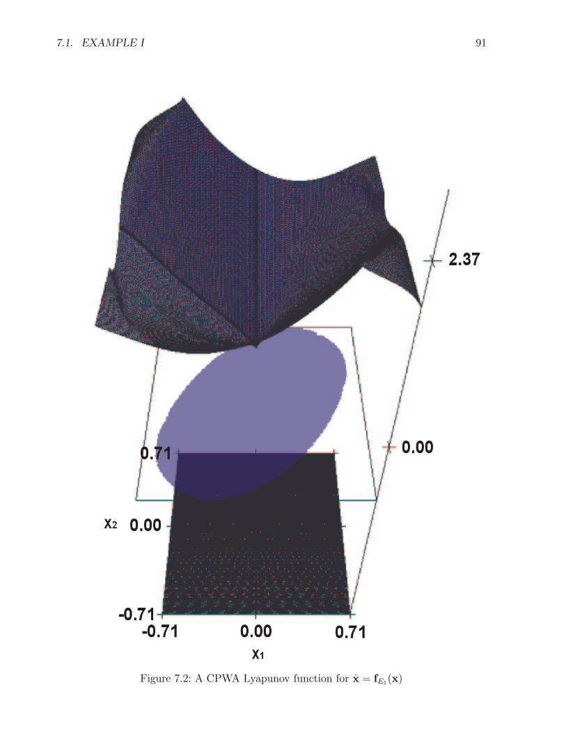
7.1. EXAMPLE I 91
Figure 7.2: A CPWA Lyapunov function for x = fE1(x)

92 CHAPTER 7. EXAMPLES
has the eigenvalues
−1
2+ i
√3
2and − 1
2− i
√3
2.
The origin is, therefore, a locally exponentially stable equilibrium point of the system (see,for example, Theorem 2.3 in Part II in [55]).
Linear Program LP2 was used to generate linear constraints for CPWA Lyapunov functionsfor the system, which CPLEXr was able to satisfy. In Figure 7.1 a CPWA Lyapunov function[−0.71, 0.71]2 −→ R, determined by its values on a 71 × 71 grid (= 5041 grid points), isplotted. The partition of the domain of the Lyapunov function is shown at the base of thegraph. The grid steps are identical for the x1- and x2-axes, 0.001 in the interval [−0.01, 0.01],0.01 in the intervals [−0.21,−0.01] and [0.01, 0.21], and 0.1 in the intervals [−0.71,−0.21]and [0.21, 0.71]. The shaded area on the partition is a lower bound of the region of attractionof the equilibrium.
In Figure 7.2 a CPWA Lyapunov function with the same domain, but determined by itsvalues on a 161×161 grid (= 25921 grid points), is drawn. The grid steps are identical for thex1- and x2-axes, 0.001 in the interval [−0.01, 0.01] and 0.01 in the intervals [−0.71,−0.01]and [0.01, 0.71]. The partition is shown at the base, but because of the small size of thesimplices they are hard to identify. A lower bound of the region of attraction is shown as ashaded area above the partition.
7.2 Example II
Consider the dynamical system x = fE2(x), where
fE2(x) :=
(x2
x1 + x2 − 3 arctan(x1 + x2)
).
This system is taken from Exercise 1.16 (2) in [21].
One easily verifies that fE2(0) = 0, that fE2 is infinitely differentiable on R2, and that itsJacobian matrix at zero,
∇fE2(0) =
(0 1−2 −2
),
has the eigenvalues
−1 + i and − 1− i.
Hence, zero is a locally exponentially stable equilibrium of the system.
Linear Program LP2 was used to generate linear constraints for a CPWA Lyapunov functionfor the system, which CPLEXr was able to satisfy. In Figure 7.3 a CPWA Lyapunov function[−1.71, 1.71]2 −→ R for a 91× 91 grid (= 8281 grid points) is plotted. As in Example I thepartition is drawn at the base and a lower bound of the region of attraction is shown as ashaded area on the partition. The grid steps are identical for the x1- and x2-axes, 0.001 inthe interval [−0.01, 0.01], 0.01 in the intervals [−0.21,−0.01] and [0.01, 0.21], and 0.1 in theintervals [−1.71,−0.21] and [0.21, 1.71].

7.2. EXAMPLE II 93
Figure 7.3: A CPWA Lyapunov function for x = fE2(x)
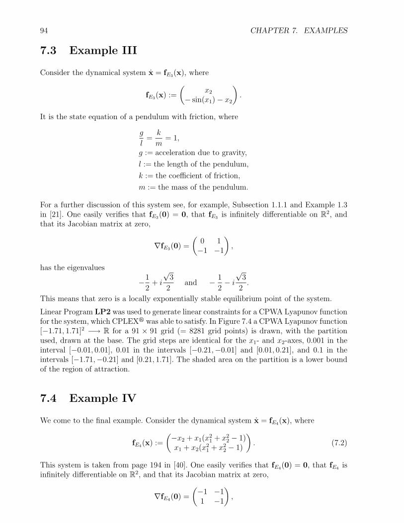
94 CHAPTER 7. EXAMPLES
7.3 Example III
Consider the dynamical system x = fE3(x), where
fE3(x) :=
(x2
− sin(x1)− x2
).
It is the state equation of a pendulum with friction, where
g
l=
k
m= 1,
g := acceleration due to gravity,
l := the length of the pendulum,
k := the coefficient of friction,
m := the mass of the pendulum.
For a further discussion of this system see, for example, Subsection 1.1.1 and Example 1.3in [21]. One easily verifies that fE3(0) = 0, that fE3 is infinitely differentiable on R2, andthat its Jacobian matrix at zero,
∇fE3(0) =
(0 1−1 −1
),
has the eigenvalues
−1
2+ i
√3
2and − 1
2− i
√3
2.
This means that zero is a locally exponentially stable equilibrium point of the system.
Linear Program LP2 was used to generate linear constraints for a CPWA Lyapunov functionfor the system, which CPLEXr was able to satisfy. In Figure 7.4 a CPWA Lyapunov function[−1.71, 1.71]2 −→ R for a 91 × 91 grid (= 8281 grid points) is drawn, with the partitionused, drawn at the base. The grid steps are identical for the x1- and x2-axes, 0.001 in theinterval [−0.01, 0.01], 0.01 in the intervals [−0.21,−0.01] and [0.01, 0.21], and 0.1 in theintervals [−1.71,−0.21] and [0.21, 1.71]. The shaded area on the partition is a lower boundof the region of attraction.
7.4 Example IV
We come to the final example. Consider the dynamical system x = fE4(x), where
fE4(x) :=
(−x2 + x1(x
21 + x2
2 − 1)x1 + x2(x
21 + x2
2 − 1)
). (7.2)
This system is taken from page 194 in [40]. One easily verifies that fE4(0) = 0, that fE4 isinfinitely differentiable on R2, and that its Jacobian matrix at zero,
∇fE4(0) =
(−1 −11 −1
),
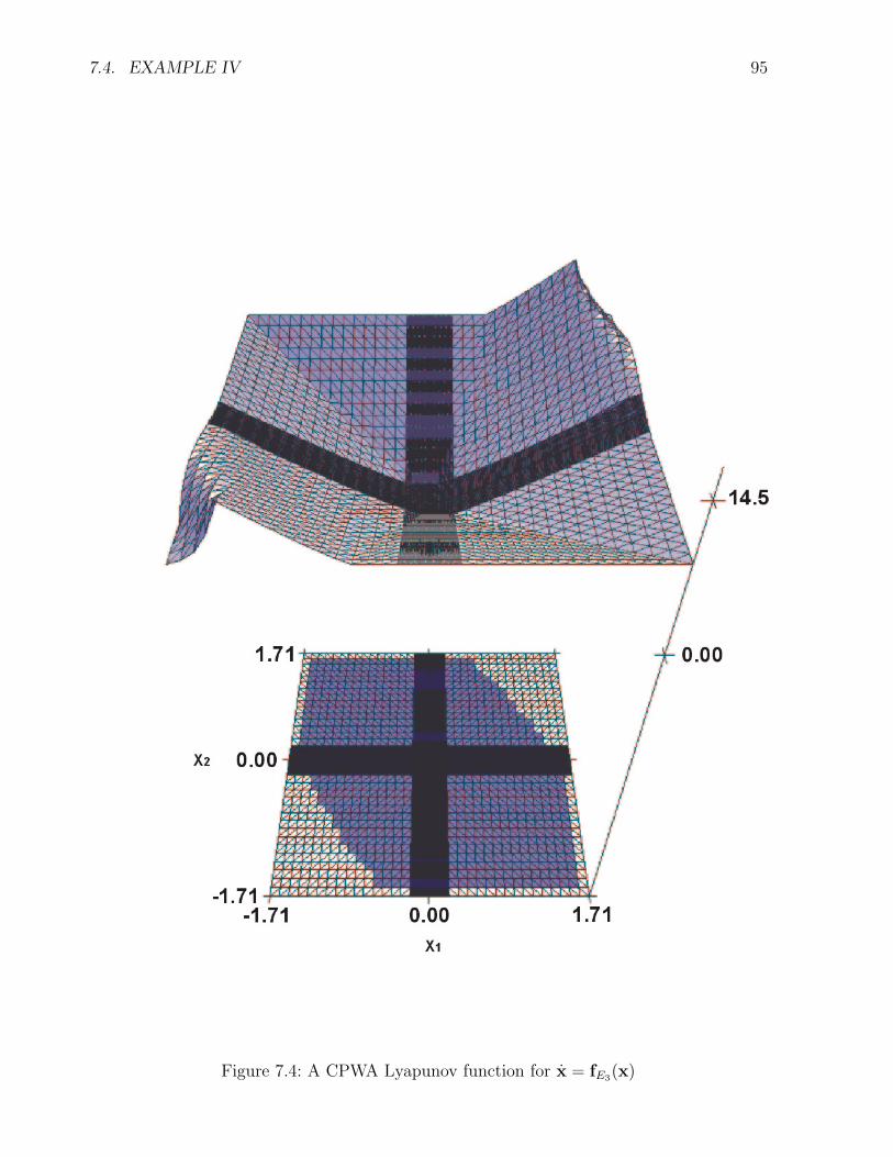
7.4. EXAMPLE IV 95
Figure 7.4: A CPWA Lyapunov function for x = fE3(x)
96 CHAPTER 7. EXAMPLES
has the eigenvalues−1 + i and − 1− i.
Hence, the origin is a locally exponentially stable equilibrium point of the system.
Let us have a closer look at the linearized system. It is well known that the differentialequation
x = ∇fE4(0)x
has the solutionφL(t, ξ) = et∇fE4
(0)ξ.
Routine calculations give
∇fE4(0) =
(−1 −11 −1
)=
(1 i1 −i
)−1(−1 + i 00 −1− i
)(1 i1 −i
).
Hence,
φL(t, ξ) = exp
[t
(1 i1 −i
)−1(−1 + i 00 −1− i
)(1 i1 −i
)]ξ
=
(1 i1 −i
)−1
exp
[t
(−1 + i 0
0 −1− i
)](1 i1 −i
)ξ
=
(1 i1 −i
)−1(e(−1+i)t 0
0 e(−1−i)t
)(1 i1 −i
)ξ
=
(e(−1+i)t+e(−1−i)t
2− e(−1+i)t−e(−1−i)t
2ie(−1+i)t−e(−1−i)t
2ie(−1+i)t+e(−1−i)t
2
)ξ
= e−t
(cos(t) − sin(t)sin(t) cos(t)
)ξ.
The obvious
‖(
cos(t) − sin(t)sin(t) cos(t)
)‖2 = 1
leads to the upper bound‖φL(t, ξ)‖2 ≤ e−t‖ξ‖2
of the solution of the linearized system. Hence, the origin is a globally 1, 1-exponentiallystable equilibrium of the linearized system.
We come back to the nonlinear system (7.2). The function V : R2 −→ R, x 7→ ‖x‖22, is a
Lyapunov function for the system. To see this, note that V (0) = 0 and that
d
dtV (φ(t, ξ))
∣∣∣∣t=0
= [∇V ](ξ) · fE4(ξ) = 2
(ξ1ξ2
)·(−ξ2 + ξ1[ξ
21 + ξ2
2 − 1]ξ1 + ξ2[ξ
21 + ξ2
2 − 1]
)(7.3)
= 2‖ξ‖22(‖ξ‖2
2 − 1),
where φ is the solution of (7.2). From this it follows that the time-derivative of V alongthe trajectories of the system is negative definite on the open unit circular disc, so theequilibrium at the origin is asymptotically stable and its region of attraction contains theopen unit circular disc (see, for example, Theorem 3.1 in [21]).
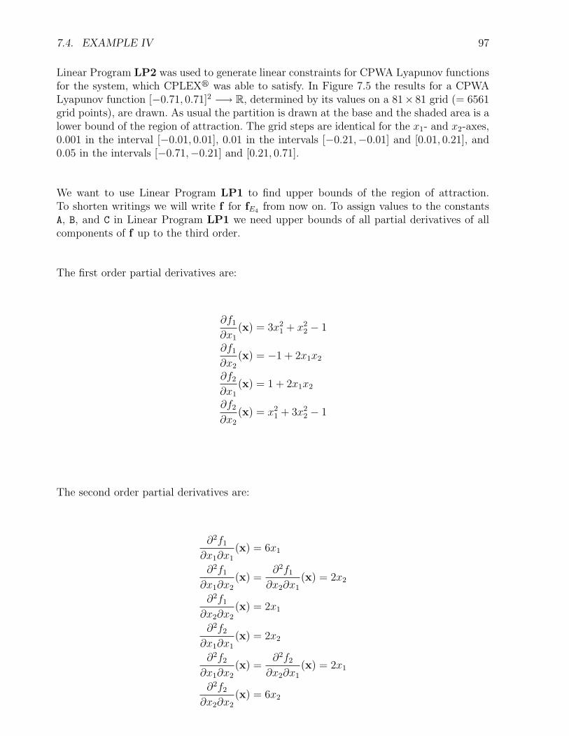
7.4. EXAMPLE IV 97
Linear Program LP2 was used to generate linear constraints for CPWA Lyapunov functionsfor the system, which CPLEXr was able to satisfy. In Figure 7.5 the results for a CPWALyapunov function [−0.71, 0.71]2 −→ R, determined by its values on a 81× 81 grid (= 6561grid points), are drawn. As usual the partition is drawn at the base and the shaded area is alower bound of the region of attraction. The grid steps are identical for the x1- and x2-axes,0.001 in the interval [−0.01, 0.01], 0.01 in the intervals [−0.21,−0.01] and [0.01, 0.21], and0.05 in the intervals [−0.71,−0.21] and [0.21, 0.71].
We want to use Linear Program LP1 to find upper bounds of the region of attraction.To shorten writings we will write f for fE4 from now on. To assign values to the constantsA, B, and C in Linear Program LP1 we need upper bounds of all partial derivatives of allcomponents of f up to the third order.
The first order partial derivatives are:
∂f1
∂x1
(x) = 3x21 + x2
2 − 1
∂f1
∂x2
(x) = −1 + 2x1x2
∂f2
∂x1
(x) = 1 + 2x1x2
∂f2
∂x2
(x) = x21 + 3x2
2 − 1
The second order partial derivatives are:
∂2f1
∂x1∂x1
(x) = 6x1
∂2f1
∂x1∂x2
(x) =∂2f1
∂x2∂x1
(x) = 2x2
∂2f1
∂x2∂x2
(x) = 2x1
∂2f2
∂x1∂x1
(x) = 2x2
∂2f2
∂x1∂x2
(x) =∂2f2
∂x2∂x1
(x) = 2x1
∂2f2
∂x2∂x2
(x) = 6x2

98 CHAPTER 7. EXAMPLES
Figure 7.5: A CPWA Lyapunov function for x = fE4(x)

7.4. EXAMPLE IV 99
The third order partial derivatives are:
∂3f1
∂x1∂x1∂x1
(x) = 6
∂3f1
∂x1∂x1∂x2
(x) =∂3f1
∂x1∂x2∂x1
(x) =∂3f1
∂x2∂x1∂x1
(x) = 0
∂3f1
∂x1∂x2∂x2
(x) =∂3f1
∂x2∂x1∂x2
(x) =∂3f1
∂x2∂x2∂x1
(x) = 2
∂3f1
∂x2∂x2∂x2
(x) = 0
∂3f2
∂x1∂x1∂x1
(x) = 0
∂3f2
∂x1∂x1∂x2
(x) =∂3f2
∂x1∂x2∂x1
(x) =∂3f2
∂x2∂x1∂x1
(x) = 2
∂3f2
∂x1∂x2∂x2
(x) =∂3f2
∂x2∂x1∂x2
(x) =∂3f2
∂x2∂x2∂x1
(x) = 0
∂3f2
∂x2∂x2∂x2
(x) = 6
For an M > 0 and a domain of the type ] −M,M [2 of f , we use these results to assignvalues to the constants a′ij, b
′ijk, and c′ijkl, i, j, k, l ∈ {1, 2}, from Linear Program LP2:
a′11 := max{4M2 − 1, 1}a′12 := 1 + 2M2
a′21 := 1 + 2M2
a′22 := max{4M2 − 1, 1}b′111 := 6M
b′112 = b′121 := 2M
b′122 := 2M
b′211 := 2M
b′212 = b′221 := 2M
b′222 := 6M
c′1111 := 6
c′1112 = c′1121 = c′1211 := 0
c′1122 = c′1212 = c′1221 := 2
c′1222 := 0
c′2111 := 0
c′2112 = c′2121 = c′2211 := 2
c′2122 = c′2212 = c′2221 := 0
c′2222 := 6
The constants a′ij, b′ijk, and c′ijkl, i, j, k, l ∈ {1, 2}, are used to assign values to the entries
aij, bij, and cij, i, j ∈ {1, 2}, of the matrices A, B, and C in Linear Program LP1. For

100 CHAPTER 7. EXAMPLES
M ≥ 1/√
2 they are:
a11 := a′11 = 4M2 − 1
a12 := a′12 := 1 + 2M2
a21 := a′21 := 1 + 2M2
a22 := a′22 = 4M2 − 1
b11 :=
√b′111
2 + b′1122 = 2
√10M
b12 :=
√b′121
2 + b′1222 = 2
√2M
b21 :=
√b′211
2 + b′2122 = 2
√2M
b22 :=
√b′221
2 + b′2222 = 2
√10M
c11 :=
√c′1111
2 + c′11122 + c′1121
2 + c′11222 = 2
√10
c12 :=
√c′1211
2 + c′12122 + c′1221
2 + c′12222 = 2
√2
c21 :=
√c′2111
2 + c′21122 + c′2121
2 + c′21222 = 2
√2
c22 :=
√c′2211
2 + c′22122 + c′2221
2 + c′22222 = 2
√10
From this,
A =
(4M2 − 1 1 + 2M2
1 + 2M2 4M2 − 1
),
B = 2√
2M
(√5 1
1√
5
),
and
C = 2√
2
(√5 1
1√
5
)follow. The constants A, B, and C, defined as the spectral norms of A, B, and C respectively,can now easily be calculated. The matrix
AT A =
((4M2 − 1)2 + (1 + 2M2)2 2(4M2 − 1)(1 + 2M2)
2(4M2 − 1)(1 + 2M2) (4M2 − 1)2 + (1 + 2M2)2
)has the eigenvalues
4M4 − 8M2 + 4 and 36M4,
where 36M4 is clearly the larger one (M ≥ 1/√
2), and the matrix
1
8M2BT B =
1
8CT C =
(6 2
√5
2√
5 6
)has the eigenvalues
6 + 2√
5 and 6− 2√
5,

7.4. EXAMPLE IV 101
where 6 + 2√
5 is the larger one. Hence,
A := ‖A‖2 =√
36M4 = 6M2,
B := ‖B‖2 = 2√
2M
√6 + 2
√5,
and
C := ‖C‖2 = 2√
2
√6 + 2
√5.
Now that we have assigned values to the constants A, B, and C, we can use Linear ProgramLP1 to generate linear constraints, capable of refuting the α,m-exponential stability of theequilibrium at the origin of (7.2) in arbitrary regions.
In all the linear programs generated the set GNh from Linear Program LP1 was defined by
GNh := {(ih, jh) ∈ R2∣∣i, j ∈ Z, |i|, |j| ≤ S},
where h = 0.01 and S is a positive integer. The results are shown in the following table:
α = 0.9 α = 0.9 α = 0.8 α = 0.8 α = 0.8m = 1.1 m = 1.2 m = 1.1 m = 1.1 m = 1.1S = 110 S = 110 S = 110 S = 120 S = 130
Feasiblesolution
No Yes Yes Yes No
Table 7.1: Results from Linear Program LP1
The simple algebraic structure of (7.2) enables an exact analysis of the system, in order tocompare the results with those of the linear programs LP1 and LP2. For this let φ be thesolution of (7.2). It follows from (7.3) that
d
dt‖φ(t, ξ)‖2
2 = 2‖φ(t, ξ)‖22(‖φ(t, ξ)‖2
2 − 1).
This differential equation is equivalent to the integral equation∫ ‖φ(t,ξ)‖22
‖ξ‖22
dy
y(1− y)= 2
∫ t
0
τdτ,
which can easily be solved
ln
(‖φ(t, ξ)‖2
2 − 1
‖ξ‖22 − 1
· ‖ξ‖22
‖φ(t, ξ)‖22
)= 2t,
i.e.
‖φ(t, ξ)‖2 =e−t‖ξ‖2√
1− ‖ξ‖22(1− e−2t)
.
From this formula for φ one immediately sees that:
102 CHAPTER 7. EXAMPLES
i) For every 0 < r ≤ 1, the origin is a 1, 1√1−r2 - exponentially stable equilibrium point
on the set {y ∈ R2∣∣‖y‖2 < r}.
ii) If ‖ξ‖2 = 1, then ‖φ(t, ξ)‖2 = 1 for all t ≥ 0.
iii) For ‖ξ‖2 > 1 the solution φ(t, ξ) has a finite escape time
tesc =1
2ln
(‖ξ‖2
2
‖ξ‖22 − 1
).
This is, of course, fully compatible with our numerical results.

Chapter 8
Concluding Remarks
In this thesis, stability properties of equilibrium points of general continuous autonomousnonlinear systems are analyzed via linear programming. The novel methods presented inthis thesis do not need the nonlinear system to be of any specific type, like piecewise affine,and show that it is possible to extract a lot of non-trivial information regarding stability byusing linear constraints.
8.1 Summary of Contributions
The main contributions of this thesis are the algorithms Linear Program LP1 and LinearProgram LP2, and the corresponding theorems Theorem I and Theorem II.
Linear Program LP1 gives explicit linear programs for dynamical systems and all constantsα > 0 and m ≥ 1, such that if there is no feasible solution of the program, then the equilib-rium of the system under consideration cannot be α,m-exponentially stable on the regionin question. The theory in Part II regarding Linear Program LP1 seems to be substantiallyclosed and complete. The bounds of the derivatives of the Lyapunov function
V (ξ) :=
∫ T
0
‖φ(τ, ξ)‖22dτ,
from the standard proof of the converse theorem on exponential stability, are fairly goodand it hardly seems possible to greatly improve them, without making major restrictionsconcerning the system in question.
Linear Program LP2 gives explicit linear programs for dynamical systems too. Such a linearprogram, generated for a particular system, has the property that a feasible solution of itdefines a CPWA Lyapunov function for the system or when D 6= ∅, a CPWA Lyapunov-likefunction which guarantees that the trajectories of the system are attracted to D. In bothcases a lower bound of the region of attraction is provided by the preimages of the Lyapunovor Lyapunov-like function. Because these are in CPWA, the calculation of their preimagesis a trivial task.
8.2 Some Ideas for Future Research
It might be interesting to use Linear Program LP1 as the evaluating step in an iterativealgorithm to estimate the region of attraction of an equilibrium of a nonlinear system. One
103

104 CHAPTER 8. CONCLUDING REMARKS
could start with a small grid around the equilibrium, such that there is a feasible solutionof the linear program generated by Linear Program LP1, and then successively add gridpoints to the grid until Linear Program LP1 generates a linear program, which no longerhas a feasible solution.
The theory regarding Linear Program LP2 wakes some very interesting questions. They can,in essence, be categorized in two types, one regarding the existence of a CPWA Lyapunov(-like) function for a particular system, and another regarding the fine tuning of the CPWALyapunov(-like) function by using the objective in the linear program.
First, we will discuss the fine tuning of the Lyapunov(-like) function. One recalls that LinearProgram LP2 states a group of linear constraints for a system, such that a feasible solutionthereof defines a CPWA Lyapunov(-like) function for the system. The objective of thelinear program is not needed. Therefore, it is logical to try to use the objective to select aLyapunov(-like) function that is well suited to the problem at hand. A well suited Lyapunov(-like) function might, for example, have one or more of the following properties:
i) It secures a large region of attraction.
ii) It secures some robustness properties of the stability.
iii) It gives bounds of the rate of convergence to equilibrium of the trajectories of thesystem.
The problem is to formulate these properties as objectives that are linear in the variablesfrom the constraints of Linear Program LP2. In [19] there is a solution concept to the thirdpoint. They define the performance of the Lyapunov function, in accordance with [35], asthe largest positive constant λ, such that
D+[V (φ(t, ξ))] ≤ −λV (φ(t, ξ)).
Then they formulate a linear objective, which gives a lower bound of λ.
We come to the second question. For the time being Linear Program LP2 is a trial-and-errorsearch method for Lyapunov functions, but can it be used to prove a constructive conversetheorem? The problem ”find values for the variables in Linear Program LP2 that satisfythe constraints” seems much simpler to solve than ”find a positive definite function that isstrictly decreasing along all trajectories of the system”. Consider the following quotationsfrom the modern literature about the value of such a theorem:
Khalil writes on page 180 in [21]:
Most of these converse theorems are provided by actually constructing auxiliaryfunctions that satisfy the conditions of the respective theorems. Unfortunately,almost always this construction assumes the knowledge of the solutions of the dif-ferential equation. Therefore, these theorems do not help in the practical searchfor an auxiliary function. The mere knowledge that a function exists is, however,better than nothing. At least we know that our search is not hopeless.
Slotline and Li write on page 120 in [44]:

8.2. SOME IDEAS FOR FUTURE RESEARCH 105
A number of interesting results concerning the existence of Lyapunov functions,called converse Lyapunov theorems, have been obtained in this regard. For manyyears, these theorems were thought to be of no practical value because, like thepreviously described theorems, they do not tell us how to generate Lyapunovfunctions for a system to be analyzed.
Vidyasagar writes on pages 235-236 in [50]:
Since the function V is constructed in terms of the solution trajectories of thesystem, the converse theorems cannot really be used to construct an explicitformula for the Lyapunov function, except in special cases (e.g., linear systems;see Section 5.4)
Currently, such a theorem is being worked on. It looks promising to combine the results fromPart II and Part III of this thesis to prove a constructive converse theorem on exponentialstability.
106 CHAPTER 8. CONCLUDING REMARKS

Bibliography
[1] R. Adams. Sobolev Spaces. Acad. Press, New York, 1975.
[2] T. Apostol. Calculus: Volume 2. John Wiley & Sons, New York, 2. edition, 1969.
[3] H. Bauer. Maß- und Integrationstheorie. de Gruyter, Berlin, 2. edition, 1990.
[4] H. Berenji. Fuzzy logic controllers. In R. Yager and L. Zadeh, editors, An Introductionto Fuzzy Logic Applications in Intelligent Systems, pages 69–96. Kluwer, Boston, 1992.
[5] S. Boyd, L. El Ghaoui, E. Feron, and V. Balakrishnan. Linear Matrix Inequalities inSystem and Control Theory. SIAM Studies in Applied Mathematics, 1994.
[6] R. Brayton and C. Tong. Stability of dynamical systems: a constructive approach.IEEE Transactions on Circuits and Systems, CAS-26:224–234, 1979.
[7] R. Brayton and C. Tong. Constructive stability and asymptotic stability of dynamicalsystems. IEEE Transactions on Circuits and Systems, CAS-27:1121–1130, 1980.
[8] U. Dini. Fondamenti per la teoria delle funzioni di variabili reali. Pisa, 1878.
[9] D. Driankov, H. Hellendorn, and R. Reinfrank. An Introduction to Fuzzy Control.Springer, Berlin, 2. edition, 1996.
[10] G. Golub and C. van Loan. Matrix Computations. The John Hopkins University Press,Baltimore, 1983.
[11] H. Grauert and I. Lieb. Differential- und Integralrechnung III. Springer, Berlin, 2.edition, 1977.
[12] W. Hahn. Stability of Motion. Springer, New York, 1967.
[13] G. Hammerlin and K.-H. Hoffmann. Numerische Mathematik. Springer, Berlin, 3.edition, 1992.
[14] M. Johansson. Piecewise Linear Control Systems. Ph.D. Thesis: Lund Institute ofTechnology, Lund, 1999.
[15] M. Johansson and A. Rantzer. Computation of piecewise quadratic Lyapunov functionsfor hybrid systems. In Proceedings of the European Control Conference ECC’97, 1997.
[16] M. Johansson and A. Rantzer. On the computation of piecewise quadratic Lyapunovfunctions. In Proceedings of the 36th IEEE Conference on Decision and Control, 1997.
107
108 BIBLIOGRAPHY
[17] P. Julian. A High Level Canonical Piecewise Linear Representation: Theory and Ap-plications. Ph.D. Thesis: Universidad Nacional del Sur, Bahia Blanca, 1999.
[18] P. Julian, A. Desages, and O. Agamennoni. High-level canonical piecewise linear rep-resentation using a simplicial partition. IEEE Transactions on Circuits and Systems,46:463–480, 1999.
[19] P. Julian, J. Guivant, and A. Desages. A parametrization of piecewise linear Lyapunovfunction via linear programming. Int. J. Control, 72:702–715, 1999.
[20] D. Karweina. Rechnergetutzte Stabilitatsanalyse fur nichtlineare zeitdiskreteRegelungssysteme, basierend auf der Methode der Konvexen Zerlegung. Ph.D. Thesis:VDI Verlag, Dusseldorf, 1989.
[21] H. Khalil. Nonlinear Systems. Macmillan, New York, 1992.
[22] H. Kiendl. Stability analysis for advanced fuzzy systems. In Proceedings of EUFIT’99(CD-ROM), Aachen, 1999. Verlag Mainz.
[23] H. Kiendl and J. Ruger. Stability analysis of fuzzy control systems using facet functions.Fuzzy Sets and Systems, 70:275–285, 1995.
[24] R. Knicker. Stability analysis of fuzzy and other nonlinear systems based on the methodof convex decomposition. In B. Reusch, editor, Computational Intelligence, Theory andApplications, pages 391–400. Springer, Berlin, 1999.
[25] R. Knicker and P. Krause. The method of convex decomposition for stability analysiswith stepwise mapping. In Proceedings of EUFIT’99 (CD-ROM), Aachen, 1999. VerlagMainz.
[26] A. Kolmogorov and S. Fomin. Introductory Real Analysis. Dover, New York, 1970.
[27] R. Kruse, J. Gebhardt, and F. Klawonn. Foundations of Fuzzy Systems. John Wiley& Sons, Chichester, 1994.
[28] A. M. Lyapunov. The general problem of the stability of motion. Int. J. Control,55:531–773, 1992.
[29] J. L. Massera. On Liapunoff’s conditions of stability. Ann. Math., 50:705–721, 1949.
[30] A. Michel, B. Nam, and V. Vittal. Computer generated Lyapunov functions for in-terconnected systems: Improved Results with Applications to Power Systems. IEEETransactions on Circuits and Systems, CAS-31:189–198, 1984.
[31] A. Michel, N. Sarabudla, and R. Miller. Stability analysis of complex dynamical sys-tems: some computational methods. Circuits and Systems Signal Processing, 1:171–202,1982.
[32] T. Mollers. Stabilitat von Fuzzy-Reglern: Analysekriterien und explizite Synthesever-fahren. Ph.D. Thesis: Shaker-Verlag, Aachen, 1998.
[33] H. Nguyen and E. Walker. A First Course in Fuzzy Logic. Chapman & Hall/CRC,Boca Raton, 2. edition, 2000.
BIBLIOGRAPHY 109
[34] Y. Ohta, H. Imanishi, L. Gong, and H. Haneda. Computer generated Lyapunov func-tions for a class of non-linear systems. IEEE Transactions on Circuits and Systems,CAS-40:343–354, 1993.
[35] A. Olas. Construction of optimal Lyapunov functions for systems with structureduncertainties. IEEE Transactions on Automatic Control, AC-39:167–171, 1994.
[36] M. Padberg. Linear Optimization and Extensions. Springer, Berlin, 2. edition, 1999.
[37] A. Polanski. Lyapunov function construction by linear programming. IEEE Trans.Autom. Control, 42:1013–1016, 1997.
[38] W. Press, S. Teukolsky, W. Vetterling, and B. Flannery. Numerical Recipes in C.Cambridge University Press, Cambridge, 2. edition, 1992.
[39] R. Rockafellar and R. Wets. Variational Analysis. Springer, Berlin, 1998.
[40] S. Sastry. Nonlinear Systems: Analysis, Stability, and Control. Springer, New York,1999.
[41] R. Schaback and H. Werner. Numerische Mathematik. Springer, Berlin, 4. edition,1992.
[42] T. Scheel. Integrale Ljapunov-Funktionen zur rechnergestutzten Stabilitatsanalyse nicht-linearer zeitdiskreter Regelungssysteme. Ph.D. Thesis: VDI Verlag, Dusseldorf, 1997.
[43] T. Scheel and H. Kiendl. Stability analysis of fuzzy and other nonlinear systems usingintegral Lyapunov functions. In Proceedings of EUFIT’95, pages 765–770, Aachen,1995. Augustinus Buchhandlung.
[44] J.-J. Slotline and W. Li. Applied Nonlinear Control. Prentice-Hall, New Jersey, 1991.
[45] M. Sugeno and G. Kang. Fuzzy modeling and control of multilayer incinerator. FuzzySets and Systems, 18:329–346, 1986.
[46] M. Sugeno and G. Kang. Structure identification of fuzzy model. Fuzzy Sets andSystems, 28:15–33, 1988.
[47] M. Sugeno and M. Nishida. Fuzzy control of model car. Fuzzy Sets and Systems,16:103–113, 1985.
[48] M. Sugeno and T. Takagi. Fuzzy identification of systems and its applications tomodeling and control. IEEE Trans. Syst. Man and Cybern., 15:116–132, 1985.
[49] M. Sugeno and K. Takana. Successive identification of a fuzzy model and its applicationsto prediction of a complex system. Fuzzy Sets and Systems, 42:315–334, 1991.
[50] M. Vidyasagar. Nonlinear System Analysis. Prentice Hall, Englewood Cliffs, 2. edition,1993.
[51] W. Walter. Analysis I. Springer, Berlin, 2. edition, 1990.
[52] W. Walter. Gewohnliche Differentialgleichungen. Springer, Berlin, 5. edition, 1993.

110 BIBLIOGRAPHY
[53] W. Walter. Einfuhrung in die Theorie der Distributionen. BI-Wiss.-Verl., Mannheim,3. edition, 1994.
[54] R. Yager and D. Filev. Essentials of Fuzzy Modeling and Control. John Wiley & Sons,New York, 1994.
[55] J. Zabczyk. Mathematical Control Theory: An Introduction. Birkhauser, Boston, 1992.