stability and control of functional differential...
TRANSCRIPT
STABILITY AND CONTROL OF FUNCTIONAL DIFFERENTIAL
EQUATIONS
A DISSERTATION
SUBMITTED TO THE DEPARTMENT OF AERONAUTICS AND
ASTRONAUTICS
AND THE COMMITTEE ON GRADUATE STUDIES
OF STANFORD UNIVERSITY
IN PARTIAL FULFILLMENT OF THE REQUIREMENTS
FOR THE DEGREE OF
DOCTOR OF PHILOSOPHY
Matthew Monnig Peet
March 2006

c© Copyright by Matthew Monnig Peet 2006
All Rights Reserved
ii

I certify that I have read this dissertation and that, in my opinion, it
is fully adequate in scope and quality as a dissertation for the degree
of Doctor of Philosophy.
Sanjay Lall Principal Adviser
I certify that I have read this dissertation and that, in my opinion, it
is fully adequate in scope and quality as a dissertation for the degree
of Doctor of Philosophy.
Matthew West
I certify that I have read this dissertation and that, in my opinion, it
is fully adequate in scope and quality as a dissertation for the degree
of Doctor of Philosophy.
Stephen Rock
I certify that I have read this dissertation and that, in my opinion, it
is fully adequate in scope and quality as a dissertation for the degree
of Doctor of Philosophy.
Geir Dullerud
iii

Approved for the University Committee on Graduate Studies.
iv
Abstract
This thesis addresses the question of stability of systems defined by differential equa-
tions which contain nonlinearity and delay. In particular, we analyze the stability
of a well-known delayed nonlinear implementation of a certain Internet congestion
control protocol. We also describe a generalized methodology for proving stability of
time-delay systems through the use of semidefinite programming.
In Chapters 4 and 5, we consider an internet congestion control protocol based on
the decentralized gradient projection algorithm. For a certain class of utility function,
this algorithm was shown to be globally convergent for some sufficiently small value
of a gain parameter. Later work gave an explicit bound on this gain for a linearized
version of the system. This thesis proves that this bound also implies stability of the
original system. The proof is constructed within a generalized passivity framework.
The dynamics of the system are separated into a linear, delayed component and a sys-
tem defined by an nonlinear differential equation with discontinuity in the dynamics.
Frequency-domain analysis is performed on the linear component and time-domain
analysis is performed on the nonlinear discontinuous system.
In Chapter 7, we describe a general methodology for proving stability of linear
time-delay systems by computing solutions to an operator-theoretic version of the
Lyapunov inequality via semidefinite programming. The result is stated in terms of
a nested sequence of sufficient conditions which are of increasing accuracy. This ap-
proach is generalized to the case of parametric uncertainty by considering parameter-
dependent Lyapunov functionals. Numerical examples are given to demonstrate con-
vergence of the algorithm. In Chapter 8, this approach is generalized to nonlinear
time-delay systems through the use of non-quadratic Lyapunov functionals.
v
Preface
This thesis covers my work done in the Networked Systems and Controls Lab at
Stanford University under the direction of Professor Sanjay Lall during the period
from August of 2002 through January of 2006. With the exception of Chapter 8,
almost all of the work presented here has been previously published or submitted to
peer-reviewed academic journals or conferences. The chapters of this thesis can be
divided into those containing original research and those containing an overview of
existing results. Specifically, Chapters 5, 7 and 8 contain original results, while most
of the rest of the chapters can be considered as survey material.
Some attempt has been made in this thesis to keep the length of the chapters
minimal in order to improve readability. The presentation style is mathematically
oriented, with specifics of numerical implementation suppressed. Proofs, when espe-
cially long, have been moved to the appendices. To maintain focus on the theoretical
contribution, in-depth treatment of various special cases has been omitted when such
treatment can be inferred from previous exposition.
vi

Contents
Abstract v
Preface vi
1 Introduction 1
1.1 Research Goals . . . . . . . . . . . . . . . . . . . . . . . . . . . . . . 1
1.2 Prior Work . . . . . . . . . . . . . . . . . . . . . . . . . . . . . . . . 3
1.3 Notation . . . . . . . . . . . . . . . . . . . . . . . . . . . . . . . . . . 7
2 Functional Differential Equations 10
2.1 Introduction . . . . . . . . . . . . . . . . . . . . . . . . . . . . . . . . 10
2.2 Definitions and the Concept of State . . . . . . . . . . . . . . . . . . 11
2.2.1 A Note on Existence of Solutions . . . . . . . . . . . . . . . . 13
2.3 Concepts of Stability . . . . . . . . . . . . . . . . . . . . . . . . . . . 14
2.3.1 Internal Stability . . . . . . . . . . . . . . . . . . . . . . . . . 14
2.3.2 Input-Output stability . . . . . . . . . . . . . . . . . . . . . . 15
2.4 Time-Delay Systems . . . . . . . . . . . . . . . . . . . . . . . . . . . 15
2.4.1 The Case of Linear Time-Delay Systems . . . . . . . . . . . . 16
2.5 Conclusion . . . . . . . . . . . . . . . . . . . . . . . . . . . . . . . . . 17
3 Stability of Functional Differential Equations 18
3.1 The Direct Method of Lyapunov . . . . . . . . . . . . . . . . . . . . . 18
3.1.1 Complete Quadratic Lyapunov Functionals . . . . . . . . . . . 19
3.2 The Method of Integral Quadratic Contraints . . . . . . . . . . . . . 20
vii
3.2.1 Theory of Integral-Quadratic Constraints . . . . . . . . . . . . 20
3.3 Conclusion . . . . . . . . . . . . . . . . . . . . . . . . . . . . . . . . . 25
4 Internet Congestion Control 26
4.1 Introduction . . . . . . . . . . . . . . . . . . . . . . . . . . . . . . . . 26
4.2 The Internet Optimization Problem . . . . . . . . . . . . . . . . . . . 27
4.3 Optimization Model . . . . . . . . . . . . . . . . . . . . . . . . . . . 29
4.4 Stability Properties . . . . . . . . . . . . . . . . . . . . . . . . . . . . 31
4.5 Recent Work . . . . . . . . . . . . . . . . . . . . . . . . . . . . . . . 32
5 Stability of Internet Congestion Control 33
5.1 Introduction . . . . . . . . . . . . . . . . . . . . . . . . . . . . . . . . 33
5.2 Reformulation of the Problem . . . . . . . . . . . . . . . . . . . . . . 34
5.2.1 Separation into subsystems . . . . . . . . . . . . . . . . . . . . 36
5.3 Input-Output Stability . . . . . . . . . . . . . . . . . . . . . . . . . . 38
5.3.1 ∆ satisfies the IQC . . . . . . . . . . . . . . . . . . . . . . . . 38
5.3.2 Properties of G . . . . . . . . . . . . . . . . . . . . . . . . . . 41
5.3.3 Stability of the Interconnection . . . . . . . . . . . . . . . . . 42
5.4 Asymptotic Stability . . . . . . . . . . . . . . . . . . . . . . . . . . . 43
5.5 Implementation . . . . . . . . . . . . . . . . . . . . . . . . . . . . . . 44
5.6 Conclusion . . . . . . . . . . . . . . . . . . . . . . . . . . . . . . . . . 44
6 Sum-of-Squares and Convex Optimization 46
6.1 Convexity and Tractability . . . . . . . . . . . . . . . . . . . . . . . . 46
6.2 Sum-of-Squares Decomposition . . . . . . . . . . . . . . . . . . . . . 47
6.3 Positivstellensatz Results . . . . . . . . . . . . . . . . . . . . . . . . . 48
6.4 Applications . . . . . . . . . . . . . . . . . . . . . . . . . . . . . . . . 51
6.4.1 Stability of Ordinary Differential Equations . . . . . . . . . . 52
6.4.2 Local Stability and Parametric Uncertainty . . . . . . . . . . 52
6.5 The SOS Representation of Matrix Functions . . . . . . . . . . . . . 54
6.6 Positivstellensatz Results for Matrix Functions . . . . . . . . . . . . . 56
6.6.1 Linear ODEs with Parametric Uncertainty . . . . . . . . . . . 57
viii

6.7 Conclusion . . . . . . . . . . . . . . . . . . . . . . . . . . . . . . . . . 58
7 Stability of Linear Time-Delay Systems 59
7.1 Introduction . . . . . . . . . . . . . . . . . . . . . . . . . . . . . . . . 59
7.2 Positive Operators . . . . . . . . . . . . . . . . . . . . . . . . . . . . 60
7.2.1 Multiplier Operators and Spacing Functions . . . . . . . . . . 62
7.2.2 Positive Finite-Rank Integral Operators . . . . . . . . . . . . . 67
7.2.3 Parameter Dependent Positive Finite-Rank Operators . . . . 71
7.3 Results . . . . . . . . . . . . . . . . . . . . . . . . . . . . . . . . . . . 71
7.3.1 The Single Delay Case . . . . . . . . . . . . . . . . . . . . . . 72
7.3.2 Examples of a Single Delay . . . . . . . . . . . . . . . . . . . 74
7.3.3 Multiple Delay Case . . . . . . . . . . . . . . . . . . . . . . . 76
7.3.4 Examples of Multiple Delay . . . . . . . . . . . . . . . . . . . 79
7.3.5 Distributed Delay Case . . . . . . . . . . . . . . . . . . . . . . 79
7.4 Conclusion . . . . . . . . . . . . . . . . . . . . . . . . . . . . . . . . . 81
8 Stability of Nonlinear Time-Delay Systems 83
8.1 Introduction . . . . . . . . . . . . . . . . . . . . . . . . . . . . . . . . 83
8.2 Delay-Dependent Stability . . . . . . . . . . . . . . . . . . . . . . . . 84
8.2.1 Single Delay Case . . . . . . . . . . . . . . . . . . . . . . . . . 84
8.2.2 Multiple Delays . . . . . . . . . . . . . . . . . . . . . . . . . . 87
8.3 Delay-Independent Stability . . . . . . . . . . . . . . . . . . . . . . . 90
8.3.1 Numerical Examples . . . . . . . . . . . . . . . . . . . . . . . 92
8.4 Conclusion . . . . . . . . . . . . . . . . . . . . . . . . . . . . . . . . . 95
A Appendix to Chapter 2 96
B Appendix to Chapter 6 105
C Appendix to Chapter 5 107
D Appendix to Chapter 7 115
ix

Bibliography 145
x
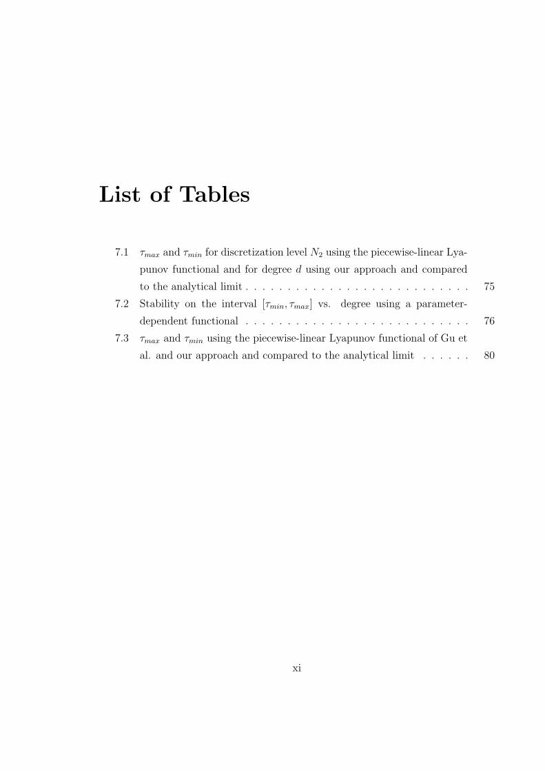
List of Tables
7.1 τmax and τmin for discretization level N2 using the piecewise-linear Lya-
punov functional and for degree d using our approach and compared
to the analytical limit . . . . . . . . . . . . . . . . . . . . . . . . . . . 75
7.2 Stability on the interval [τmin, τmax] vs. degree using a parameter-
dependent functional . . . . . . . . . . . . . . . . . . . . . . . . . . . 76
7.3 τmax and τmin using the piecewise-linear Lyapunov functional of Gu et
al. and our approach and compared to the analytical limit . . . . . . 80
xi
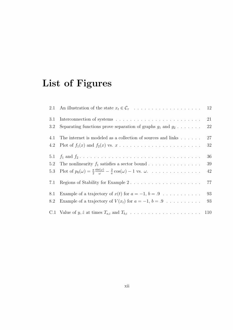
List of Figures
2.1 An illustration of the state xt ∈ Cτ . . . . . . . . . . . . . . . . . . . 12
3.1 Interconnection of systems . . . . . . . . . . . . . . . . . . . . . . . . 21
3.2 Separating functions prove separation of graphs g1 and g2 . . . . . . . 22
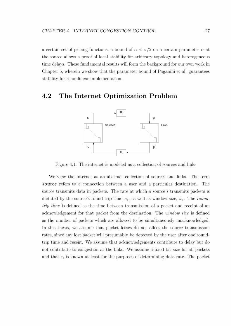
4.1 The internet is modeled as a collection of sources and links . . . . . . 27
4.2 Plot of f1(x) and f2(x) vs. x . . . . . . . . . . . . . . . . . . . . . . . 32
5.1 f1 and f2 . . . . . . . . . . . . . . . . . . . . . . . . . . . . . . . . . . 36
5.2 The nonlinearity f1 satisfies a sector bound . . . . . . . . . . . . . . . 39
5.3 Plot of p0(ω) = π2
sin(ω)ω
− 2π
cos(ω)− 1 vs. ω. . . . . . . . . . . . . . . 42
7.1 Regions of Stability for Example 2 . . . . . . . . . . . . . . . . . . . . 77
8.1 Example of a trajectory of x(t) for a = −1, b = .9 . . . . . . . . . . . 93
8.2 Example of a trajectory of V (xt) for a = −1, b = .9 . . . . . . . . . . 93
C.1 Value of y, z at times Ta,i and Tb,i . . . . . . . . . . . . . . . . . . . . 110
xii

Chapter 1
Introduction
1.1 Research Goals
The analysis of nonlinear systems is a subject of much recent interest. Although
linearization is a well-established approach to analysis, results obtained in this man-
ner are always, at best, local. When considering changes in critical systems such as
the Internet, the guarantee of convergence associated with a global stability result
carries significant weight. Furthermore, some dynamical systems, such as are found
in biology or high performance aircraft, are dominated by nonlinear behavior. In
such cases, the practical value of linear analysis is limited. Apart from nonlinearity,
the study of decentralized systems and systems with delay is also the topic of much
active research. Communications systems, an issue of significant current interest, are
often decentralized and, by virtue of their geographic reach, inevitably contain delay.
Earth based telescopes are currently being built which consist of thousands of mirror
segments; each individually actuated but required to move in a coordinated manner.
Such systems are difficult to model using a state space of reasonable dimension.
The recent development of efficient algorithms for optimization on the cone of
positive semidefinite matrices has created a fundamental shift in how research is con-
ducted. Specifically, semidefinite programming has been widely adopted in control
1
CHAPTER 1. INTRODUCTION 2
theory and has led to a greater understanding of linear finite dimensional central-
ized systems. Unfortunately, this same understanding has not yet been extended to
nonlinear, infinite dimensional or decentralized systems. In fact, many critical ques-
tions in analysis and control of these systems have been shown to be NP-hard. The
goal of our research at Stanford has been to find new ways to address these types of
problems. One approach is to expand the definition of solution. Instead of giving a
single necessary and sufficient condition, expressible as a semidefinite program, one
can construct a nested sequence of sufficient conditions, of increasing accuracy, which
converge to a necessary and sufficient condition and are expressible as semidefinite
programs. Examples of this technique as well as others can be found in the chapters
of this thesis.
Internet Congestion Control The application which has motivated much of the
research in this thesis has been stability analysis of proposed protocols for Internet
congestion control. The analysis of congestion control protocols has received much
attention recently. This work has been motivated by concern about the ability of
current protocols to ensure stability and performance as the number of users and
amount of bandwidth continues to increase. Although the protocols that have been
used in the past have performed well as the Internet has increased in size, as capac-
ities and delays increase instability will become a problem. In our work, we have
considered global stability with delay of congestion control protocols which attempt
to solve a distributed network optimization problem. These systems are described by
differential equations with delay and contain non-static nonlinearity. Because of the
nonlinearity and delays, proving convergence is difficult. By combining frequency and
time domain techniques using a generalized passivity framework, in Chapters 4 and 5,
we have shown for certain protocols that global stability with delay holds under the
same conditions as local stability. Condensed versions of these results also appear in
publication in [35] and [36]. These tight bounds, verified by experimental evidence,
allow one to accurately predict when congestion control will fail.

CHAPTER 1. INTRODUCTION 3
An Approach to Analysis and Synthesis Our research at Stanford has produced
a number of new results and tools concerning the analysis of systems with delay, non-
linearity and decentralized structure. Specifically, in Chapter 7, we have proposed
two new types of refutation which can be used to construct the positive quadratic
Lyapunov-Krasovskii functionals necessary for stability of linear time-delay systems.
Furthermore, we have shown how these refutations can be parameterized using the
space of positive semidefinite matrices. This has resulted in a nested sequence of
sufficient conditions, of increasing accuracy and expressible as semidefinite programs,
which prove stability of linear time-delay systems. Thus for any desired level of ac-
curacy, these results give a condition, expressible as a semidefinite program, which
will test stability to that level of accuracy. These results appear in publication in [37]
and [38]. In addition, because of the structure of the refutations, in Chapter 8 we have
also been able to generalize these results to time-delay systems with nonlinearities.
Some of these results appear in publication in [34].
1.2 Prior Work
The contents of this thesis utilize results from a number of different areas of research.
A complete survey of the results in any one of these fields would be beyond the scope
of this document. In this section we briefly list some landmark contributions which
have directly influenced the direction of our research.
Stability Theory Early results include the work of the Russian mathematician A.
M. Lyapunov [25], who, in 1892, standardized the definition of stability and gener-
alized the potential energy work of Lagrange [21] to systems of ordinary differential
equations of the form x(t) = f(x(t)). In the century that has followed, the use of
Lyapunov functions to prove stability has become commonplace and is known alter-
natively as the “Direct method of Lyapunov” or “Lyapunov’s second method”.
In the 1960’s, the input-output approach to stability analysis emerged as an al-
ternative to Lyapunov’s method. This approach was motivated by the development

CHAPTER 1. INTRODUCTION 4
of complicated electronic systems for which a detailed analysis of the stability of the
internal states was impractical. The work was pioneered by Sandberg [42, 42] and
Zames [51, 52] and can be found in such works as [48] and [9]. The input-output
framework was of practical importance for a number of primary reasons. First, it
could be used with “black-box” frequency sweeping techniques to quickly determine
properties of complicated linear systems even when those systems contained internal
delay. In addition, these frequency-domain properties could then be used to predict
the stability of the interconnection of systems through the use of concepts such as
passivity and small-gain. Development of the input-output framework has had some
relatively recent advances with the introduction of the theory of “Integral Quadratic
Constraints”(IQCs) by Rantzer and Megretskii[40]. This work on IQCs generalizes
the passivity framework by formulating stability conditions which allow for the use of
a broad class of multipliers. This work will be discussed in more depth in Chapter 3.
Semidefinite Programming The first stability problem to be posed as a linear
matrix inequality(LMI) can be attributed to Lyapunov himself, who stated that the
system
x(t) = Ax(t)
is stable if and only if there exists a P ≥ 0 such that
AT P + PA < 0.
Of course, in the absence of algorithms for this LMI, Lyapunov was forced to express
this conditional analytically as the unique solution, P , for arbitrary Q > 0, of the
Lyapunov equation AT P +PA = −Q. The analysis of LMIs arising in control theory
through the use of analytical solutions was continued in the 1940’s and 1950’s by the
work of Lur’e, Postnikov, and others in the Soviet Union.
The first general method for the solution of LMIs was developed in the 1960’s by
Kalman, Yakubovich, and others. The famous positive-real or KYP lemma showed
that a certain class of LMI problems could be solved graphically by considering a
frequency domain inequality. Today, of course, the KYP lemma is currently used

CHAPTER 1. INTRODUCTION 5
more often in the opposite sense, i.e. to convert a frequency-domain inequality to a
semidefinite program. The LMI associated with the KYP lemma was later shown to
admit an analytic solution through use of the algebraic Riccati equation(ARE).
The most significant advance in the solution of LMI problems was the recognition
in the 1970’s that many LMIs could be expressed as convex optimization problems
which could be solved using recently developed efficient numerical algorithms for
linear programming. Thus the use of analytic solutions to LMI problems was replaced
by semidefinite programming which is defined as optimization over the convex cone
of positive semidefinite matrices.
The algorithms for numerical optimization which were first used to solve LMI
problems were originally developed to solve linear programming problems of the fol-
lowing form where the inequality is defined by the positive orthant.
max cT y :
Ay ≤ b
The solution of linear programming problems was first addressed by the devel-
opment of the Simplex algorithm by G. Dantzig in the mid-40’s. This algorithm
performed well when applied to most problems but was shown to fail in certain
special cases. Concern about this “worst-case” complexity prompted the search for
what we now refer to as polynomial-time algorithms, which have provable bounds on
worst-case performance. The first such polynomial-time algorithm was introduced
by Khachiyan in 1979 and is referred to as the ellipsoid algorithm. This algorithm,
however, proved inferior to the Simplex algorithm in most practical cases. The first
major improvement over the Simplex algorithm was developed in 1984, when N. Kar-
makar proposed a new type of algorithm which used what we now refer to as an
“interior-point” method. This algorithm was also of polynomial-time complexity but
performed far better than the ellipsoid algorithm in practice. The final hurdle towards
numerical solution of LMI problems was overcome in 1988, when Nesterov and Ne-
mirovskii developed interior point algorithms which applied directly to semidefinite
programming problems. Today, semidefinite programming programs can be solved
CHAPTER 1. INTRODUCTION 6
simply and efficiently using interior-point solvers such as SeDuMi [45] combined with
user-friendly interfaces such as Yalmip. A summary of standard LMI problems in
control theory can be found in the seminal work by Boyd et al. [4].
Recently, the success of semidefinite programming in addressing problems in con-
trol has led to research into whether these algorithms can be applied to convex prob-
lems in polynomial optimization. Polynomial optimization problems arise in many
areas of nonlinear systems analysis and control and this topic will be covered in
significant depth in Chapter 6.
Internet Congestion Control The origins of research interest in Internet conges-
tion control from a mathematical perspective can be traced back to the the paper by
Kelly et al. [18], wherein the the congestion control problem was first cast as a de-
centralized optimization problem. This paper showed that certain congestion control
protocols would converge to the global optimum in the absence of delay through the
use of a Lyapunov argument. Subsequently, in Low and Lapsley [23], it was shown
that the dynamics of the delayed Internet model with a certain class of control algo-
rithms could be interpreted as a decentralized implementation of the asynchronous
gradient projection algorithm to solve the dual to the network optimization problem
thus showing global convergence to optimality for sufficiently small step size. How-
ever, no global bound for the step size was given in this paper, making practical
interpretation difficult. This work was followed by the paper by Paganini et al. [29],
wherein it was shown that with a certain set of pricing functions, a uniform bound of
α < π/2 on a certain gain parameter α at the source allows a proof of local stability
for arbitrary topology and heterogeneous time delays. The uniform bound of α < π/2
was shown to imply global stability for heterogeneous time delays in a more limited
topology in [35] and [36]. All these results are discussed in more depth in Chapters 4
and 5.
Time-Delay Systems In 1963, the potential energy methods of Lagrange and
Lyapunov were generalized to systems of functional differential equations by N. N.
Krasovskii [20]. Since this time, many computationally tractable sufficient conditions
CHAPTER 1. INTRODUCTION 7
have been given for stability of both linear and nonlinear time-delay systems, all
with varying degrees of conservatism. An overview of some of these results can be
obtained from survey materials such as are found in [13, 14, 19, 28]. These results
can be grouped into analysis either in the frequency-domain or in the time-domain.
Frequency-domain techniques can be applied to linear systems only and typically at-
tempt to determine whether all roots of the characteristic equation of the system lie
in the left half-plane. This approach is complicated by the transcendental nature of
the characteristic equation, which imply the existence of a possibly infinite number
of roots. Time-domain techniques generally use Lyapunov-based analysis. In the lin-
ear case, the Lyapunov approach benefits from the existence of an operator-theoretic
version of Lyapunov’s inequality, the existence of a positive solution to which is neces-
sary and sufficient for stability. Computing solutions to this inequality, however, has
historically been problematic. A main contribution of this thesis is to show how the
operator-theoretic Lyapunov equation can be solved directly using semidefinite pro-
gramming. This work is described in Chapter 7 and the references [37] and [38]. We
note that one attempt to solve the Lyapunov equation by considering piecewise-linear
functions was made in a series of papers by Gu et al. and is summarized in [13].
1.3 Notation
The following are used throughout this thesis.
Vector Spaces In this thesis, we use the following standard notation. Rn×m denotes
the space of real n×m matrices. Sn denotes the space of symmetric n×n matrices. Let
R+ := x ∈ R | x ≥ 0 . Let C(I) denote the set of continuous functions u : I → Rn
where I ⊂ R. We say f ∈ C(I) is bounded if there exists some b ∈ R+ such that
‖f(θ)‖2 ≤ b for all θ ∈ I. We use Cτ to denote the Banach space of continuous
functions u ∈ C([−τ, 0]) with norm ‖u‖ = supt∈[−τ,0] ‖u(t)‖2.
Definition 1. For a given τ > 0, x ∈ C([a, b)), and t ∈ [a + τ, b], where b > a + τ ,
define xt ∈ Cτ by xt(θ) = x(t + θ) for θ ∈ [−τ, 0].
CHAPTER 1. INTRODUCTION 8
L2(−∞,∞) is the Hilbert space of Lebesgue measurable real vector-valued func-
tions x : R→ Rn with inner-product 〈u, v〉2 =∫∞−∞ u(t)T v(t)dt. L2 denotes L2[a,∞) =
x ∈ L2(−∞,∞) | x(t) = 0 for all t < 0 and is a Hilbert subspace of L2(−∞,∞).
Similarly, L2[a, b] denotes the restriction of L2(−∞,∞) to the interval [a, b]. Through-
out, the dimensions of x(t) for x ∈ L2 should be clear from context and are not
explicitly stated. We will occasionally also associate with Cτ an inner product space
equipped with the inner product associated with L2. Thus for x, y ∈ Cτ , 〈x, y〉denotes the L2 inner product. L2 denotes the Hilbert space of complex vector-
valued functions on the imaginary axis, x : jR → Cn with inner-product 〈u, v〉2 =12π
∫∞−∞ u(jω)∗v(jω)dω. L∞ denotes the Banach space of matrix-valued functions on
the imaginary axis, G : jR→ Cm×n with norm ‖G‖∞ = ess supω∈R σ(G(jω)
)where
σ(G(jω)) denotes the maximum singular value of G(jω). For a given τ > 0, let M2
denote the product space Rn × L2[−τ, 0] endowed with the inner product
〈x, y〉 := xT1 y1 + 〈x2, y2〉2,
where we associate with x ∈ M2 a pair (x1, x2) where x1 ∈ Rn and x2 ∈ L2[−τ, 0].
Maps and Operators An operator A on an inner-product space X is defined to
be positive if 〈x,Ax〉 ≥ 0 for all x ∈ X. A function x : R → R is said to be
absolutely continuous if for any integer N and any sequence t1, . . . , tN , we have∑N−1k=1 |x(tk) − x(tk+1)| → 0 whenever
∑N−1k=1 |tk − tk+1| → 0. PT is the truncation
operator such that if y = PT z, then y(t) = z(t) for all t ≤ T and y(t) = 0 otherwise.
L2e denotes the space of functions such that for any T > 0 and y ∈ L2e, we have
PT y ∈ L2. We also make use of the space W2 = y : y, y ∈ L2 with inner product
〈x, y〉W2 = 〈x, y〉L2 + 〈x, y〉L2 and extended space W2e = y : y, y ∈ L2e. A causal
operator H : L2e → L2e is bounded if H(0) = 0 and if it has finite gain, defined as
‖H‖ = supu∈L2 6=0
‖Hu‖‖u‖

CHAPTER 1. INTRODUCTION 9
u denotes the either the Fourier or Laplace transform of u, depending on u. We
will also make use of the following specialized set of transfer functions which define
bounded linear operators on L2. A is defined to be those transfer functions which are
the Laplace transform of functions of the form
g(t) =
h(t) +∑N
i=1 giδ(t− ti) if t ≥ 0
0 otherwise
where h ∈ L1, gi ∈ R and ti ≥ 0.
Real Algebraic Geometry Denote by R[x] the ring of scalar polynomials in vari-
ables x. Denote by Rn×m[x] the set of n by m matrices with scalar elements in R[x].
Let Sn[x] denote the set of symmetric n by n matrices with elements in R[x] and
define Snd [x] to be the elements of Sn[x] of degree d or less. Let PY ⊂ R[x] denote
the convex cone of scalar polynomials which are non-negative on Y . Let P+ ⊂ R[x]
denote the convex cone of globally non-negative scalar polynomials. Let SYn ⊂ Sn[x]
denote the convex cone of elements M ∈ Sn[x] such that M(x) ≥ 0 for all x ∈ Y . Let
S+n denote the convex cone of elements M ∈ Sn[x] such that M(x) ≥ 0 for all x. We
let Zd[x] denote the(
n+dd
)-dimensional vector of monomials in n variables x of degree
d or less. Define Znd [x] := In ⊗ Zd[x], where In is the identity matrix in Sn. Finally,
we note that for the sake of notational convenience, we will often use the expression
M(x) ∈ X to indicate that the function M ∈ X for some set of functions X. This
will hopefully not cause substantial amounts of confusion.
Chapter 2
Functional Differential Equations
2.1 Introduction
The best way to introduce the concept of a functional differential equation is through
the use of an example.
Example 1: Perhaps the most easily understood example of a system defined by a
functional differential equation is that of the dynamics of taking a shower. Specifically,
define δT (t) to be the difference between water temperature and body temperature
at time t. We assume that the typical bather controls the water temperature by
turning the hot-water knob at rate ω(t), proportional to the difference between water
temperature and body temperature so that ω(t) = −αδT (t). Ideally, the position of
the hot water knob is directly proportional to the temperature of the water coming
from the head, δT (t) = βω(t). In this case, we have the following ordinary differential
equation.
δT (t) = αω(t) = −αβδT (t)
This is a linear, time-invariant system and consequently we know that limt→∞ δT (t) =
0 for any any initial condition δT (0) and any positive value of α. However, as most
people know, there is occasionally a delay between action on the hot-water knob and
change of temperature at the head. This delay occurs because hot water mixed at
10
CHAPTER 2. FUNCTIONAL DIFFERENTIAL EQUATIONS 11
the knob must pass through a length of pipe before arrival at the shower head. We
assume that the delay, τ , is constant and can be calculated as τ = L/v; where L is
the linear distance from the tap to the head and v is the rate of the water flowing in
the pipe. The simplest description of the delayed system is given as follows.
δT (t) = −αβδT (t− τ)
It can be shown[14] that a system of this form is stable in the region αβ ∈(0, π
2τ) and unstable outside of this region. Thus we conclude that in the presence of
delay, any bather will get scalded if sufficiently impatient. The reason that a large
proportional feedback gain fails in the shower example is that the temperature of the
water at the head does not provide an adequate representation of the state of the
system. In order to exactly predict exactly how the water temperature will evolve
over time, one needs to know the water temperature, T (θ, t), at every point θ in the
pipe from the knob to the head for some time t. This information precisely defines
the state of the system at time t. Because the state at time t, T (·, t) is a function,
the dynamics of a shower are defined by a function of a function or a functional.
In fact, the dynamics given above represent a simplification of the more difficult
problem of fluid flow described by partial differential equations. We are able to rep-
resent the system using such a simple model only because the controller and observer
are highly structured so that control and observation take place only at discrete points
in the flow. Such simplified models are quite common and are collectively known as
time-delay systems.
2.2 Definitions and the Concept of State
To begin, we define the following.
Definition 2. Suppose we are given a τ ≥ 0 and map f : Cτ × R+ → Rn. We say
that a function x ∈ C([−τ, b)) is a solution on [−τ, b) to the functional differential
equation defined by f with initial condition x0 ∈ Cτ if x is differentiable, x(θ) = x0(θ)
CHAPTER 2. FUNCTIONAL DIFFERENTIAL EQUATIONS 12
for θ ∈ [−τ, 0] and the following holds for t ≥ 0.
x(t) = f(xt, t) (2.1)
In this thesis, we make use of two different concepts of state space. The first,
and perhaps the most common is the Banach space Cτ , equipped with the supremum
norm. In this scenario, the state of the system is simply the trajectory of the system
over the past τ seconds of time. It is in this space that we will define solution maps
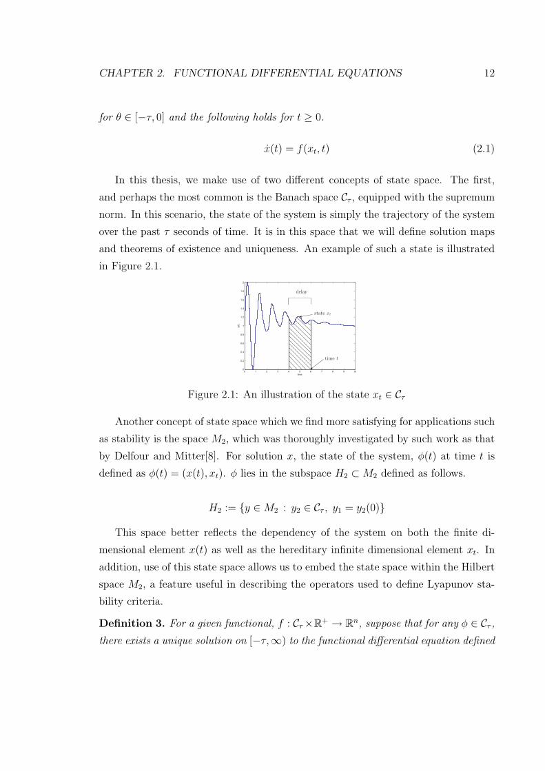
and theorems of existence and uniqueness. An example of such a state is illustrated
in Figure 2.1.
0 1 2 3 4 5 6 7 8 9 100
0.2
0.4
0.6
0.8
1
1.2
1.4
1.6
1.8
2
time
x(t
)
delay
state
time
xt
t
Figure 2.1: An illustration of the state xt ∈ Cτ
Another concept of state space which we find more satisfying for applications such
as stability is the space M2, which was thoroughly investigated by such work as that
by Delfour and Mitter[8]. For solution x, the state of the system, φ(t) at time t is
defined as φ(t) = (x(t), xt). φ lies in the subspace H2 ⊂ M2 defined as follows.
H2 := y ∈ M2 : y2 ∈ Cτ , y1 = y2(0)
This space better reflects the dependency of the system on both the finite di-
mensional element x(t) as well as the hereditary infinite dimensional element xt. In
addition, use of this state space allows us to embed the state space within the Hilbert
space M2, a feature useful in describing the operators used to define Lyapunov sta-
bility criteria.
Definition 3. For a given functional, f : Cτ×R+ → Rn, suppose that for any φ ∈ Cτ ,
there exists a unique solution on [−τ,∞) to the functional differential equation defined

CHAPTER 2. FUNCTIONAL DIFFERENTIAL EQUATIONS 13
by f . Define the solution map Gf : Cτ → C([−τ,∞)) by y = Gf (φ) where y is the
solution to the functional differential equation defined by f with initial condition φ.
For the time-invariant case, where f(xt, t) = f(xt), we define the following, which
maps the evolution of the state.
Definition 4. For a given solution map, Gf , define the flow map Γf : Cτ × [0, b) →Cτ by ξ = Γf (φ, ∆t) if ξ = y∆t where y = Gf (φ).
The solution map, Gf , and flow map, Γf , provide convenient notation for express-
ing the evolution of the system over time. The following result gives conditions under
which the solution map is well-defined in the time-varying case.
2.2.1 A Note on Existence of Solutions
In this subsection, we give a theorem which provides conditions for the existence and
uniqueness of solutions defined on C([−τ,∞)).
Theorem 5. Suppose a functional f : Cτ × R+ → Rn satisfies the following.
• There exists a K1 > 0 such that
‖f(x, t)− f(y, t)‖2 ≤ K1‖x− y‖Cτ for all x, y ∈ Cτ , t ≥ 0
• There exists a K2 > 0 such that
‖f(0, t)‖ ≤ K2 for all t ≥ 0
• f(x, t) is jointly continuous in x and t. i.e. for every (x, t) and ε > 0, there
exists a η > 0 such that
‖x− y‖Cτ + ‖t− s‖ ≤ η ⇒ ‖f(x, t)− f(y, s)‖ ≤ ε.

CHAPTER 2. FUNCTIONAL DIFFERENTIAL EQUATIONS 14
Then for any φ ∈ Cτ , there exists a unique x ∈ C[−τ,∞) such that x is differentiable
for t ≥ 0, x(t) = φ(t) for t ∈ [−τ, 0] and
x(t) = f(xt, t) for all t ≥ 0
See Appendix A for Proof.
By use of Theorem, 5, we can show that if a functional, f , satisfies a global Lips-
chitz continuity condition, then for any initial condition there exists a unique solution
to the functional differential equation defined by f which is defined on [−τ,∞). In this
case the solution map and, in the time-invariant case, the flow map are well-defined.
2.3 Concepts of Stability
In this section we define stability of a functional differential equation.
2.3.1 Internal Stability
Two concepts of stability will be used in this thesis. The first, internal stability,
defines stability as a property of solutions of a functional differential equation for
arbitrary initial conditions. The second, input-output stability, is used to define
stability of an operator and describes the relationship between inputs and outputs.
In this subsection we give a definition of internal stability.
Definition 6. Assume that f satisfies f(0, t) = 0. The solution map Gf , defined by
f , is stable on X ⊂ Cτ if
(i) Gfx is bounded for any x ∈ X
(ii) Gf is continuous at 0 with respect to the supremum norm on C([−τ,∞)) and
Cτ .
This is the usual notion of Lyapunov stability, which states that for all ε > 0 there
exists δ > 0 such that ‖y‖ < δ implies ‖Gfy‖ < ε.
CHAPTER 2. FUNCTIONAL DIFFERENTIAL EQUATIONS 15
Definition 7. The solution map Gf defined by f is asymptotically stable on
X ⊂ Cτ if it is stable on X and y = Gfx0 implies limt→∞ y(t) = 0 for any x0 ∈ X.
Definition 8. The solution map, Gf , is globally stable if it is stable on Cτ
Definition 9. The solution map, Gf , is globally asymptotically stable if it is
asymptotically stable on Cτ .
Note: For a system defined by a linear functional, global stability is equivalent
to stability on any open neighborhood of the origin. See, for example [13, 19].
2.3.2 Input-Output stability
We can associate with a functional, f , an input-output system.
Definition 10. For functional f and function g, let y = Ψf,gu if y(t) = g(x(t)) for
t ∈ R+ where x = Gf (0) and
f(xt, t) = f(xt, t) + u(t).
We can now define input-output stability directly in terms of properties of the
operator Ψ.
Definition 11. For normed spaces X, Y , the operator Ψ is Y stable on X if it defines
a single-valued map from X to Y and there exists some β such that ‖Ψu‖Y ≤ β‖u‖X
for all u ∈ X.
Note: We refer to X stability on X as simply X stability.
2.4 Time-Delay Systems
So far, we have only considered the general case of a dynamic system defined by
a functional. In this section, we identify a specific class of functional differential
equation which will be of particular importance throughout this thesis.

CHAPTER 2. FUNCTIONAL DIFFERENTIAL EQUATIONS 16
Definition 12. We say that a functional, f , defines a Time-Delay System if f
can be represented using a function p : Rn(K+1)+1 → Rn in the following way where
τi > τi−1 for i = 1, . . . , K and τ0 = 0.
f(xt) =
∫ 0
−τK
p(xt(−τ0), xt(−τ1), · · · , xt(−τK), xt(θ), θ)dθ
Stability of Time-Delay systems are generally classified using the following defini-
tions.
Definition 13. A Time-Delay System is Delay-Independent Stable if it is stable
for arbitrary τi ∈ R for i = 1 . . . K.
Definition 14. A Time-Delay System is Delay-Dependent Stable on X if it is
stable for τi ∈ Xi for i = 1 . . . K where the Xi are compact subsets of R.
2.4.1 The Case of Linear Time-Delay Systems
In this subsection, we consider the special case of linear time-delay systems. Specif-
ically, we consider functionals which can be expressed in the following form, where
τi > τi−1 for i = 1, . . . , K and τ0 = 0.
f(xt) =K∑
i=0
Aix(t− τi) +
∫ 0
−τK
A(θ)x(t + θ)dθ (2.2)
Here Ai ∈ Rn×n and A : R→ Rn×n is bounded on [−τK , 0]. The following lemma,
combined with Theorem 5 shows that elements of this class of system admit a unique
solution for every initial condition x0 ∈ CτK.
Lemma 15. Let
f(x, t) :=K∑
i=1
Ajx(t− τi) +
∫ 0
−τK
A(θ)x(t− θ)dθ

CHAPTER 2. FUNCTIONAL DIFFERENTIAL EQUATIONS 17
Where A(θ) is bounded on [−τ, 0]. Then there exists some K > 0 such that
‖f(x, t)− f(y, t)‖2 ≤ K‖x− y‖Cτ
See appendix for Proof.
By using Lemma 15, we can associate with linear systems of this form a well-
defined solution map Gf and flow map Γf .
2.5 Conclusion
In this chapter, we have introduced various concepts associated with functional dif-
ferential equations. These concepts include the state of the system, the solution map
and stability in both the internal and input-output framework. We will make use of
these definitions throughout the remainder of this thesis.
Chapter 3
Stability of Functional Differential
Equations
In this chapter, we introduce two methods of proving stability of functional differ-
ential equations. The first, which can be used to prove internal stability, uses a
generalization of Lyapunov theory to functional differential equations. The second
method, which is used to prove input-output stability, is a generalization of the notion
of passivity.
3.1 The Direct Method of Lyapunov
Consider a solution map Gf defined by a functional f . We consider the state of the
system at time t to be defined by an element xt ∈ Cτ . Standard Lyapunov theory,
however, is defined using functions of the form V (x(t)). Such functions capture
only part of the energy of the state, xt, i.e. that part stored in xt(0). Therefore,
any stability condition derived from such functions will be inherently conservative.
An attempt to address this conservatism was made by Krasovskii [20] through the
introduction of Lyapunov functionals which depend on elements of Cτ .
Definition 16. Let V : Cτ → R be a continuous function such that V (0) = 0. For a
given flow map, Γf , defined by solution map, Gf , define the upper Lie derivative of V
18
CHAPTER 3. STABILITY OF FUNCTIONAL DIFFERENTIAL EQUATIONS19
as follows.
V (φ) := lim suph→0+
1
h[V (Γf (φ, h))− V (φ)]
The following theorem follows from Gu [13].
Theorem 17. Let Ω ⊂ Cτ contain an open neighborhood of the origin. Let f : Ω → Rn
be continuous and take bounded sets of Ω into bounded sets of Rn. Let V : Cτ → Rbe a continuous function such that V (0) = 0. Let u, v, w : R+ → R+ be continuous
non-decreasing functions such that u(s), v(s) > 0 for s 6= 0 and u(0) = v(0) = 0.
Suppose that the following holds for any φ ∈ Ω.
u(‖φ(0)‖) ≤ V (φ) ≤ v(‖φ‖)V (φ) ≤ −w(|φ(0)|)
Then the solution map, Gf , defined by f is stable on some open neighborhood of the
origin. If w(s) > 0 for s > 0, then the system is asymptotically stable on some
open neighborhood of the origin. If Ω = Cτ and lims→∞ = ∞, then Gf is globally
asymptotically stable.
3.1.1 Complete Quadratic Lyapunov Functionals
There have been a number of results concerning necessary and sufficient conditions
for stability of linear time-delay systems in terms of the existence of quadratic func-
tionals. These results are significant in that they allow us to restrict our search for
a Lyapunov-Krasovskii functional to a specific class without introducing any conser-
vatism. Consider a linear functional of the following form.
f(xt) =K∑
i=0
Aix(t− τi) +
∫ 0
−τK
A(θ)x(t + θ)dθ (3.1)
We now make the additional assumption that A is continuous on [−τK , 0]. The
following comes from Gu et al. [13].
Definition 18. We say that a functional V : Cτ → R is of the complete quadratic
type if there exists a matrix P ∈ Sn and matrix-valued functions Q : R → Rn×n,
CHAPTER 3. STABILITY OF FUNCTIONAL DIFFERENTIAL EQUATIONS20
S : R → Sn and R : R2 → Rn×n where R(θ, η) = R(η, θ)T such that the following
holds.
V (φ) = φ(0)T Pφ(0) + 2φ(0)T
∫ 0
−τK
Q(θ)φ(θ)dθ
+
∫ 0
−τK
φ(θ)T S(θ)φ(θ)dθ +
∫ 0
−τK
∫ 0
−τK
φ(θ)T R(θ, η)φ(η)dθdη
Theorem 19. Suppose the system defined by a linear functional of the form (3.1) is
asymptotically stable. Then there exists a complete quadratic functional V and η > 0
such that the following holds for all φ ∈ Cτ .
V (φ) ≥ η‖φ(0)‖2 and V (φ) ≤ −η‖φ(0)‖2
Furthermore, the matrix-valued functions which define V can be taken to be continuous
everywhere except possibly at points θ, η = −τi for i = 1, . . . , K − 1.
3.2 The Method of Integral Quadratic Contraints
The method of integral quadratic constraints of IQCs is a method of proving stability
of the interconnection of stable operators.
3.2.1 Theory of Integral-Quadratic Constraints
Consider the following interconnection of operators.
Definition 20. Let G be a linear operator with transfer function G ∈ A and let the
operator ∆ : L2 → L2 be causal and bounded. Define inputs f ∈ W2 and g ∈ L2. The
interconnection of G and ∆, denoted ΦF,G, is defined by (y, u) = Φ(f, g) where y
and u are defined as follows.
y = Gu + f
u = ∆y + g

CHAPTER 3. STABILITY OF FUNCTIONAL DIFFERENTIAL EQUATIONS21
g
f
y
G
+
+ u
É
Figure 3.1: Interconnection of systems
Definition 21 (Jonsson [16], p71). The interconnection of G and ∆, ΦG,∆, is
well-posed if for every pair (f, g) with f ∈ W2 and g ∈ L2, there exists a solution
u ∈ L2e, y ∈ W2e and the map (f, g) → (y, u) is causal.
If the interconnection of ∆ and G is well posed, then the interconnection defines
an operator ΦG,∆ : W2 × L2 → W2e × L2e. In this thesis, we use a result by Rantzer
and Megretski [40] which can be interpreted as generalization of the classical notion
of passivity. Recall the the following classical passivity theorem from e.g. Desoer and
Vidyasagar(p. 182, [9])
Theorem 22. The interconnection of ∆ and G is L2 stable on L2 if there exists some
ε > 0 such that for any x ∈ L2,
〈∆x, x〉 ≥ 0
〈x,Gx〉 ≤ −ε‖x‖
Now given bounded linear transformations Π1, Π2, define the following functional
〈x, y〉Π :=
⟨Π1
[x
y
], Π2
[x
y
]⟩
Ignoring technical details for the moment, the result by Rantzer and Megretski
states that the interconnection of ∆ and G is stable if there exists an ε > 0 such that
CHAPTER 3. STABILITY OF FUNCTIONAL DIFFERENTIAL EQUATIONS22
for any x ∈ L2,
〈x, ∆x〉Π ≥ 0
〈Gx, x〉Π ≤ −ε‖x‖
This idea of generalized passivity is motivated from a geometric standpoint by the
topological separation argument, introduced by Safonov [41]. Consider the following
definition of an operator graph.
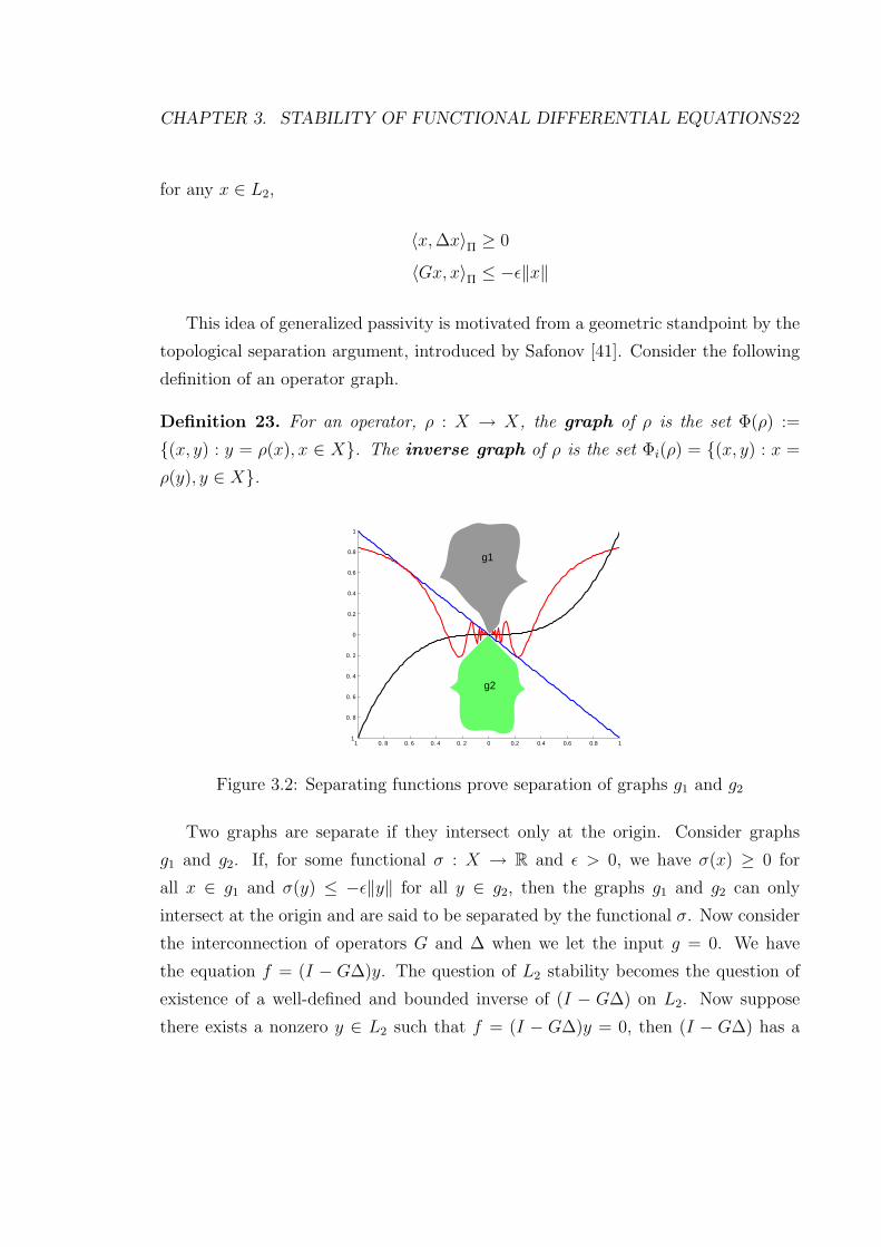
Definition 23. For an operator, ρ : X → X, the graph of ρ is the set Φ(ρ) :=
(x, y) : y = ρ(x), x ∈ X. The inverse graph of ρ is the set Φi(ρ) = (x, y) : x =
ρ(y), y ∈ X.
1 0. 8 0. 6 0. 4 0. 2 0 0.2 0.4 0.6 0.8 1 1
0. 8
0. 6
0. 4
0. 2
0
0.2
0.4
0.6
0.8
1
g1
g2
Figure 3.2: Separating functions prove separation of graphs g1 and g2
Two graphs are separate if they intersect only at the origin. Consider graphs
g1 and g2. If, for some functional σ : X → R and ε > 0, we have σ(x) ≥ 0 for
all x ∈ g1 and σ(y) ≤ −ε‖y‖ for all y ∈ g2, then the graphs g1 and g2 can only
intersect at the origin and are said to be separated by the functional σ. Now consider
the interconnection of operators G and ∆ when we let the input g = 0. We have
the equation f = (I − G∆)y. The question of L2 stability becomes the question of
existence of a well-defined and bounded inverse of (I − G∆) on L2. Now suppose
there exists a nonzero y ∈ L2 such that f = (I − G∆)y = 0, then (I − G∆) has a

CHAPTER 3. STABILITY OF FUNCTIONAL DIFFERENTIAL EQUATIONS23
nontrivial kernel and thus can not have a bounded inverse. To ensure that (I −G∆)
has a trivial kernel, we will consider the graph of G and the inverse graph of ∆. The
following well-known result shows that separation of the graph and inverse graph of
interconnected operators is necessary for stability.
Theorem 24. Let f = (I −G∆)y. The following are equivalent
• (I −G∆)y = 0 ⇒ y = 0
• Φ(G) ∩ Φi(∆) = 0
Proof. (⇐) If there exists a y 6= 0 such that (I −G∆)y = 0 then let x = ∆y. Thus
[x
Gx
]=
[∆y
y
]∈ Φ(G) ∩ Φi(∆)
(⇒) If there exists y, x 6= 0 such that
[x
Gx
]=
[∆y
y
]
then (I −G∆)y = y −G∆y = Gx−G∆y = G∆y −G∆y = 0
Although the separation of graphs is clearly necessary for most definitions of sta-
bility, it is unclear under what additional conditions separation may also be sufficient
for L2 stability. The result by Rantzer and Megretiski gives a particular class of
functionals for which graph separation is sufficient for stability on L2. Many classical
theorems concerning the stability of the interconnection of operators can be viewed
as proving the separation of graphs and inverse graphs by using these type of sepa-
rating functionals. For example, the small gain theorem can be expressed using the
separating functional σ((x, y)) = ‖x‖ − k‖y‖ for some k > 0. Similarly, classical
passivity can be expressed using the functional σ((x, y)) = 〈x, y〉. The complete class
of functionals shown by [40] to be sufficient for L2 stability is given by Definition 25.
Definition 25 (Rantzer [40]). The mapping σ : L2 → R is quadratically con-
tinuous if for every δ > 0, there exists a ηδ such that the following holds for all
CHAPTER 3. STABILITY OF FUNCTIONAL DIFFERENTIAL EQUATIONS24
x1, x2 ∈ L2.
|σ(x1)− σ(x2)| ≤ ηδ‖x1 − x2‖2 + δ‖x2‖2
This class includes the small gain and passivity functions. Furthermore, for any
bounded linear transformations Π1, Π2, the function σ(w) = 〈Π1w, Π2w〉 is quadrat-
ically continuous. In this thesis we use the following generalization of the work by
Rantzer and Megretski as presented in the thesis work by Jonsson [16].
Definition 26. Let ΠB : jR→ Cn×n be a bounded and measurable function that takes
Hermitian values and λ ∈ R. We say that ∆ satisfies the IQC defined by ΠB, λ,
if there exists a positive constant γ such that for all y ∈ W2 and v = ∆y ∈ L2,
1
2π
∫ ∞
−∞
[y(jω)
v(jω)
]∗ΠB(jω)
[y(jω)
v(jω)
]dω + 2〈v, λy〉 ≥ −γ|y(0)|2
Theorem 27. Assume that
1. G is a linear causal bounded operator with sG(s), G(s) ∈ A
2. For all κ ∈ [0, 1], the interconnection of κ∆ and G is well-posed
3. For all κ ∈ [0, 1], κ∆ satisfies the IQC defined by ΠB, λ
4. There exists η > 0 such that for all ω ∈ R[G(jω)
I
]∗ (ΠB(jω) +
[0 λjω∗
λjω 0
])[G(jω)
I
]≤ −ηI
Then the interconnection of G and ∆ is W2 × L2 stable on W2 × L2.

CHAPTER 3. STABILITY OF FUNCTIONAL DIFFERENTIAL EQUATIONS25
3.3 Conclusion
In this chapter, we have introduced two methods of constructing stability proofs of
internal and input-output stability, respectively. In the rest of this thesis, we shall
show how these methods can be applied to prove stability of different kinds of time-
delay systems.
Chapter 4
Internet Congestion Control
4.1 Introduction
The analysis of Internet congestion control protocols has received much attention re-
cently. Explicit mathematical modeling of the Internet has allowed analysis of existing
protocols from a number of different theoretical perspectives and has generated some
suggestions for improvement to current protocols. This work has been motivated by
concern about the ability of current protocols to ensure stability and performance of
the Internet as the number of users and amount of bandwidth continues to increase.
Although the protocols that have been used in the past have performed remarkably
well as the Internet has increased in size, analysis [22] indicates that as capacities and
delays increase, instability will become a problem.
The purpose of this chapter is to outline the development of a mathematical the-
ory of internet congestion control. Most of the recent research activity in Internet
congestion control protocols can be traced back to the the paper by Kelly et al. [18],
wherein the the congestion control problem was first cast as a decentralized optimiza-
tion problem. Subsequently, in Low and Lapsley [23], it was shown that the dynamics
of the Internet with a certain class of control algorithms could be interpreted as a
decentralized implementation of the gradient projection algorithm to solve the dual
to the network optimization problem, thus showing global convergence to optimality
for sufficiently small step size. Finally, in Paganini et al. [29] it was shown that with
26
CHAPTER 4. INTERNET CONGESTION CONTROL 27
a certain set of pricing functions, a bound of α < π/2 on a certain parameter α at
the source allows a proof of local stability for arbitrary topology and heterogeneous
time delays. These fundamental results will form the background for our own work in
Chapter 5, wherein we show that the parameter bound of Paganini et al. guarantees
stability for a nonlinear implementation.
4.2 The Internet Optimization Problem
fR
Rb
Sources Links
x y
pq
Figure 4.1: The internet is modeled as a collection of sources and links
We view the Internet as an abstract collection of sources and links. The term
source refers to a connection between a user and a particular destination. The
source transmits data in packets. The rate at which a source i transmits packets is
dictated by the source’s round-trip time, τi, as well as window size, wi. The round-
trip time is defined as the time between transmission of a packet and receipt of an
acknowledgement for that packet from the destination. The window size is defined
as the number of packets which are allowed to be simultaneously unacknowledged.
In this thesis, we assume that packet losses do not affect the source transmission
rates, since any lost packet will presumably be detected by the user after one round-
trip time and resent. We assume that acknowledgements contribute to delay but do
not contribute to congestion at the links. We assume a fixed bit size for all packets
and that τi is known at least for the purposes of determining data rate. The packet
CHAPTER 4. INTERNET CONGESTION CONTROL 28
transmission rate, xi, at source i can be controlled by the window size according to
wi = xiτi. (4.1)
The term link refers to a single congested resource such as a router. Packets
arriving at a link enter an entrance queue. A link can process packets in the queue
at some rate capacity cj. If too many data packets arrive in a given period of time,
the size of the queue may grow and some packets may experience a queueing delay
while in the queue. In this thesis, we assume that the dynamics from this variable
queueing delay are negligible and we only model the delay due to the fixed propagation
time. Links must also be able to feed back information. This can be done either
through the ECN bit in the packet header, through packet dropping schemes or
through measurement of variations in queueing delay at the source. The value of
the congestion indicator at link j is denoted pj. We also assume that the congestion
indicator received at each source is the summation of the indicators of all links in the
source’s route. This value is denoted qi.
Sources and links are related by routing tables which specify the route or set of
links, Ji through which the packets from source i to its destination must pass. The
rate of packets received at a link j is then the sum of the rates of all sources using
that link and is denoted by yj. The set of users for link j is denoted Ij. Ignoring
delay for the moment, we have the following equations.
y = Rx, q = RT p,
where
Rji =
1 if source i uses link j
0 otherwise

CHAPTER 4. INTERNET CONGESTION CONTROL 29
4.3 Optimization Model
The following model for optimizing flow rates in a network was proposed by Kelly et
al. [18].
maximizeN∑i
Ui(xi)
subject to x ≥ 0, Rx ≤ c
Assume that the Ui are continuously differentiable strictly concave non-decreasing
functions. If all sources utilize at least one link, then the problem has a unique
optimum. Note that, as N increases, the problem becomes progressively more difficult
to solve using a centralized algorithm. We now consider the dual problem with dual
variable p ∈ RM , where M is the number of links, which is given by
minimize h(p)
subject to p ≥ 0
where the dual function h is given by
h(p) = maxx≥0
∑i
(Ui(xi)
)− pT (Rx− c)
=∑
i
(Ui
(xopt,i(p)
))− pT (Rxopt(p)− c)
xopt,i(p) = max0, U ′−1i (
∑j
Rj,ipj)
= max0, U ′−1i (qi(p))
q(p) = RT p
The map U ′−1i : R+ → R∪∞ is well defined since U ′
i ∈ C and Ui is strictly concave.
We would like to construct a dynamical system which converges to the solution of
the dual problem. One such system is given by the gradient projection algorithm. In
CHAPTER 4. INTERNET CONGESTION CONTROL 30
discrete-time, this is
pj(t + 1) = max0, pj(t)− γjDjh(p(t)),
where Dj denotes the partial derivative with respect to the j’th argument and γj is
the step size. Since the Ui are strictly concave, h(p) is continuously differentiable
with the following derivatives [2].
Djh(p) = cj −∑i∈Ij
xopt,i
= cj − yopt,j(p)
yopt(p) = Rxopt(p).
If γ is sufficiently small, the discrete-time gradient projection algorithm will converge
to the solution of the dual problem [23]. Because of convexity of the problem, strong
duality implies that xopt(p) will converge to the unique optimum of the primal prob-
lem. A continuous-time implementation of this algorithm in the network framework
is as follows.
pj(t) =
γj(yj(t)− cj) pj(t) > 0
max0, γj(yj(t)− cj) pj(t) ≤ 0
xi(t) = max0, U ′−1i (qi(t))
y(t) = Rx(t), q(t) = RT p(t)
γj now denotes a gain parameter, corresponding to step-size in discrete time. This
algorithm has the remarkable property that it is decentralized, corresponding to the
separable structure of the constraints. pj is computed at each of M links. Link j
requires only knowledge of yj to compute this value. xi is computed at each of N
sources. Source i requires only knowledge of qi to compute this value.
CHAPTER 4. INTERNET CONGESTION CONTROL 31
4.4 Stability Properties
To ensure that the continuous-time gradient projection algorithm will converge when
implemented with the current internet framework, we must also consider the delay in
transmitting packets from the source to the link and then receiving acknowledgements
at the source. The delay from source i to link j is denoted τ fij and the delay from
link j to source i is denoted τ bij. For any source i, the total round trip time is fixed,
i.e. τi = τ fij + τ b
ij for all j ∈ Ji. We express these delays in the frequency domain
by replacing the entries of the routing matrix R with forward and backward delay
transfer functions Rf and Rb, giving
y(s) = Rf (s)x(s), q(s) = Rb(s)T p(s)
Rfji(s) =
e−τfijs if source i uses link j
0 otherwise
Rbji(s) =
e−τbijs if source i uses link j
0 otherwise
The work by Paganini et al. [29] introduced a class of utility functions under which
this system was shown to have a stable linearization about its positive equilibrium
point for a fixed gain parameter γj = 1/cj. This class was given by the set of Ui such
thatd
dqi
U ′−1i (qi) = − αi
Miτi
U ′−1i (qi),
where Mi is a bound on the number of links in the path of source i and αi < π/2. In
particular, the choice of
Ui(x) =Miτi
αi
x
(1− ln
x
xmax,i
),
with restricted domain x ≤ xmax,i was suggested in [29] as a strictly concave util-
ity function such that the function U ′−1i (q) = xmax,ie
− αiMiτi
q ≥ 0 has the necessary
derivative.
CHAPTER 4. INTERNET CONGESTION CONTROL 32
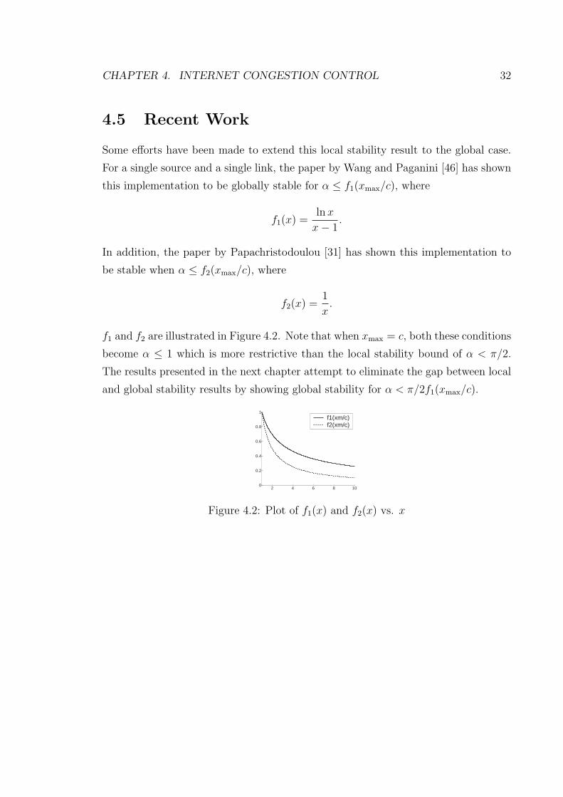
4.5 Recent Work
Some efforts have been made to extend this local stability result to the global case.
For a single source and a single link, the paper by Wang and Paganini [46] has shown
this implementation to be globally stable for α ≤ f1(xmax/c), where
f1(x) =ln x
x− 1.
In addition, the paper by Papachristodoulou [31] has shown this implementation to
be stable when α ≤ f2(xmax/c), where
f2(x) =1
x.
f1 and f2 are illustrated in Figure 4.2. Note that when xmax = c, both these conditions
become α ≤ 1 which is more restrictive than the local stability bound of α < π/2.
The results presented in the next chapter attempt to eliminate the gap between local
and global stability results by showing global stability for α < π/2f1(xmax/c).
2 4 6 8 100
0.2
0.4
0.6
0.8
1
f1(xm/c)f2(xm/c)
Figure 4.2: Plot of f1(x) and f2(x) vs. x

Chapter 5
Stability of Internet Congestion
Control
5.1 Introduction
In this chapter, we extend some of the linear stability results of Paganini et al. [29]
discussed in the previous chapter to the dynamics of a nonlinear implementation.
Many algorithms have been proposed for Internet congestion control, some of which
have been shown to be globally stable in the presence of delays, nonlinearities and
discontinuities. These proofs can be grouped into several categories according to
methodology. In particular, Lyapunov-Razumhikin theory has been used to show
global stability in [49, 7, 15, 46, 47], Lyapunov-Krasovskii functionals have been used
to show global stability in [1, 26, 31, 30] and an input-output approach was taken
in [46, 10]. In all of these cases, stability has been proven with varying degrees of
conservatism with respect to restrictions on system parameters or delays.
In general, stability analysis of nonlinear, discontinuous differential equations with
delay is quite difficult. Although frequency domain techniques have been shown to
be effective when applied to linear systems with delay, these tools fail in the presence
of nonlinearity. In addition, although time-domain analysis of nonlinear finite di-
mensional systems has had some success, analysis of the infinite dimensional systems
associated with delay has been more problematic. In this thesis, we are able to obtain
33

CHAPTER 5. STABILITY OF INTERNET CONGESTION CONTROL 34
improved results by decomposing the nonlinear, discontinuous, delayed system into an
interconnection of a linear system with delay and a nonlinear, discontinuous system
without delay. We analyze the subsystems separately and prove a passivity result for
each. One benefit of such an approach is that it allows us to use frequency-domain
arguments in addressing the infinite dimensional linear system. We can then use
time-domain arguments in the analysis of the single state nonlinear system. These
individual results are then be combined using the newly developed generalized pas-
sivity framework of Rantzer and Megretski as outlined in Chapter 3. This approach
yields improved results by allowing us to decompose the original difficult problem
into simpler subproblems, each of which may be solved with less conservatism. To
apply the passivity framework of Rantzer and Megretski to the internet congestion
control problem, we must first transform what is essentially a question of internal
stability into a problem posed in the input-output framework. Furthermore, because
input-output stability and internal stability are not equivalent, once a passivity result
has been proven, we must use further analysis to show that this implies asymptotic
stability. All these issues are addressed in the following sections.
5.2 Reformulation of the Problem
In this section we reformulate the question of internal stability of the proposed con-
gestion control algorithm as a question of input-output stability of the interconnection
of a linear system with delay and a nonlinear system without delay. This approach
was motivated, in part, by the work of Wang[46] and Jonsson[17]. If we consider the
problem of a single link and a single source, then from the development in Chapter 4,
we have that y(t) = x(t − τ f ) and q(t) = p(t − τ b) where τ f + τ b = τ . Given an
initial condition x0 ∈ Cτ , the dynamics can now be summarized as p(t) = x0(t) for

CHAPTER 5. STABILITY OF INTERNET CONGESTION CONTROL 35
t ∈ [−τ, 0] and the following for t ≥ 0.
p(t) =
xmax
ce−
ατ
p(t−τ) − 1 p(t) > 0
max0, xmax
ce−
ατ
p(t−τ) − 1 p(t) ≤ 0(5.1)
x(t) = xmaxe−α
τp(t−τb) (5.2)
Since the dynamics of Equation (5.1) are decoupled from those of (5.2) and stability
of x follows from that of p, we need only consider stability of Equation (5.1). Now
consider the equilibrium point of Equation (5.1), p0 = τα
ln xmax
c. As is customary, we
change to variable z, where z(t) = p(t)−p0 so that the origin is an equilibrium point.
Now we have z(t) = x0(t)− p0 for t ∈ [−τ, 0] and the following for t ≥ 0.
z(t) =
e−ατ
z(t−τ) − 1 z(t) > −p0
max0, e−ατ
z(t−τ) − 1 z(t) ≤ −p0
(5.3)
For convenience and efficiency of presentation, we will refer to the solution map
defined by Equation (5.3) as A : Cτ → C. Implicit in these dynamics is the constraint
z(t) ≥ −p0. If we assume that any initial condition will satisfy this constraint, we
can include the constraint in the dynamics without altering the solution map. For
convenience, we define the following bounded continuous functions.
f1(y) = mine
ατ
y − 1, eατ
p0 − 1
f2(y) = max0, f1(y)
fc(x, y) =
f1(y) if x > −p0
f2(y) otherwise
These functions are illustrated in Figure 5.1. We now have the following equation
for t ≥ 0.
z(t) = fc(z(t),−z(t− τ)) (5.4)

CHAPTER 5. STABILITY OF INTERNET CONGESTION CONTROL 36
−4 −2 0 2 4−2
−1
0
1
2
3
f 1(x)
x−4 −2 0 2 4
−2
−1
0
1
2
3
f 2(x)
x
Figure 5.1: f1 and f2
Before proceeding, we must mention well-posedness of the solution map, A. We
use a method of steps. Given any absolutely continuous solution z(t) on some interval
[T1, T1 + τ ], we observe that z(t) = fc(z(t), z(t − τ)) = fc(z(t), t) is a function only
of time and state z(t) for the interval [T1 + τ, T1 + 2τ ]. From boundedness of the fc,
continuity with respect to z(t−τ) and noting upper semi-continuity of the associated
differential inclusion with respect to z(t), we can now establish via Fillipov [11][p77]
the existence and uniqueness of a continuous solution z(t) over the interval [T1 +
τ, T1 + 2τ ]. Assuming a continuous initial condition, this implies the existence and
uniqueness of the solution map A : Cτ → C.
5.2.1 Separation into subsystems
Equation (5.4) is a delay-differential equation defined by a nonlinear, discontinuous
function. To aid in the analysis, we will reformulate the problem as the interconnec-
tion of two subsystems where the W2 stability on W2 × L2 stability of this intercon-
nection implies asymptotic stability on X of the original formulation for some set X.
Define the map G by w = Gu if
w(t) =
∫ t
t−τ
u(θ)dθ.
Note that G is a linear operator which can be represented by the convolution with
g(t) = step(t) − step(t − τ) ∈ L1. This implies that G ∈ A. Moreover, G can be
represented in the frequency domain by G(s) = 1−e−τs
swhich implies G is a bounded
CHAPTER 5. STABILITY OF INTERNET CONGESTION CONTROL 37
operator on L2 since ‖G(jω)‖∞ = τ . In addition, sG(s) ∈ A since it can be repre-
sented by convolution with δ(t)− δ(t− τ). Define the map ∆z by z = ∆zy if z(0) = 0
and
z(t) = fc
(z(t), y(t)− z(t)
).
We define the map ∆ by v = ∆y if v(t) = z(t) where z = ∆zy. Addressing well-
posedness, if y ∈ W2, then y is absolutely continuous on any finite interval(See p. 25
in Jonsson [16]). From boundedness of fc, continuity with respect to y(t), and upper
semi-continuity of the associated differential inclusion with respect to z(t), we can
again establish the existence and uniqueness of an absolutely continuous solution z
and thus of the map ∆z. Well-posedness of ∆ follows immediately. Further properties
of ∆ will be derived in later sections.
If we now form the interconnection of G and κ∆ for κ ∈ [0, 1], as defined above
with a single input f ∈ W2, we can construct a map from input f to outputs y, u. For
convenience and efficiency of presentation, we will denote the interconnection map
for κ = 1 by B : W2 → W2e × L2e. Furthermore, for κ = 1 we denote the map from
input f to internal variable z by Bz. For t ≤ 0, we let u(t) = y(t) = z(t) = f(t) = 0
and for t ≥ 0, the interconnection dynamics combine as follows.
u(t) = κz(t)
y(t) =
∫ t
t−τ
u(t)dt + f(t)
= κ(z(t)− z(t− τ)
)+ f(t)
z(t) = fc(z(t), y(t)− z(t))
= fc(z(t), f(t)− κz(t− τ)− (1− κ)z(t))
As before, from continuity with respect to f(t) and z(t−τ), upper semi-continuity
with respect to z(t) and boundedness of fc, we can conclude existence and uniqueness
of z ∈ L2e. Since z has bounded derivative and z(t) = 0 for t ≤ 0, we now have that
the map Bz : W2 → W2e is well-posed. Furthermore, this implies that y ∈ W2e and
u ∈ L2e which yields well-posedness of the interconnection for any κ ∈ [0, 1] and

CHAPTER 5. STABILITY OF INTERNET CONGESTION CONTROL 38
specifically of the map B : W2 → W2e × L2e.
5.3 Input-Output Stability
In this section we use the IQC defined by ΠB, λ = 2π, where
ΠB =
[0 β
β − 4π− 2
]
and β = α/(αmaxτ) to establish W2 × L2 stability on W2 of the interconnection for
any τ ≥ 0, 0 < α < π/2αmax. Here we define
αmax = ln(xmax/c)/((xmax/c)− 1
).
5.3.1 ∆ satisfies the IQC
In this subsection we show that if α > 0, then ∆ and consequently κ∆ are bounded
and satisfy the IQC defined by ΠB, λ = 2π
for all κ ∈ [0, 1]. The methods used in this
subsection were motivated by those in Jonnson [17] and Wang [46]. For γ = 4β/π > 0,
we prove the following for all y ∈ W2, v = ∆y.
1
2π
∫ ∞
−∞
[y(jω)
v(jω)
]∗ [0 β
β − 4π− 2
][y(jω)
v(jω)
]+
4
π〈v, y〉
≥ −γ|y(0)|2
By Parseval’s equality, this is equivalent to
2
π〈v, y − v〉+ 〈v, βy − v〉 ≥ −γ
2|y(0)|2
A critical result used in the analysis of this section is the existence of a sector
bound on the nonlinearity f1 and consequently on f2.
Lemma 28. 0 ≤ fi(x)x ≤ βx2 for i = 1, 2 where β = eατ p0−1
p0.

CHAPTER 5. STABILITY OF INTERNET CONGESTION CONTROL 39
4 2 0 2 4 2
1
0
1
2
3
f 1(x)
x
Figure 5.2: The nonlinearity f1 satisfies a sector bound
See Appendix C for Proof.
This key feature is illustrated in Figure 5.2.
Lemma 29. If v = ∆y with y ∈ W2, then
1. v ∈ L2 with norm bound β‖y‖,
2. 〈v, βy − v〉 ≥ 0
Proof. We start by noting the following.
fc(x, y) =
f1(y) if x > −p0 or y ≥ 0
0 otherwise
As a consequence of the above sector bounds, we have
fc(x, y)2 ≤ βyfc(x, y).
Let z = ∆zy, then this implies
z(t)2 = fc
(z(t), y(t)− z(t)
)z(t)
≤ β(y(t)− z(t)
)z(t)
CHAPTER 5. STABILITY OF INTERNET CONGESTION CONTROL 40
Now for any T ≥ 0, we have
‖PT v‖2 =
∫ T
0
v(t)2dt =
∫ T
0
z(t)2dt
≤ β
∫ T
0
z(t)(y(t)− z(t))dt
= β
∫ T
0
z(t)y(t)dt− β
2(z(T )2 − z(0)2)
≤ β〈PT z, y〉 (5.5)
≤ β‖PT z‖‖y‖ = β‖PT v‖‖y‖
Therefore, ‖PT v‖ ≤ β‖y‖ for all T ≥ 0. Thus v ∈ L2 with norm bounded by β‖y‖.Statement 2 follows from line 5.5 by letting T →∞.
Lemma 30. Let z = ∆zy with y ∈ W2, then limt→∞ z(t) = 0.
See Appendix C for Proof.
Lemma 31. If v = ∆y with y ∈ W2, then 〈v, y − v〉 ≥ −β|y(0)|2.
See Appendix C for Proof.
Lemma 32. κ∆ satisfies the IQC defined by ΠB, λ = 2π
for any κ ∈ [0, 1]
Proof. By Lemmas 29 and 31, we have the following.
1
2π
∫ ∞
−∞
[y(jω)
v(jω)
]∗ [0 β
β − 4π− 2
][y(jω)
v(jω)
]+
4
π〈v, y〉
=4
π〈v, y − v〉+ 2〈v, βy − v〉
≥ −4β
π|y(0)|2
We conclude as a consequence that κ∆ satisfies the IQC defined by ΠB, λ = 2π
for
CHAPTER 5. STABILITY OF INTERNET CONGESTION CONTROL 41
any κ ∈ [0, 1], since
2
π〈κv, y − κv〉+ 〈κv, βy − κv〉
≥ κ( 2
π〈v, y − v〉+ 〈v, βy − v〉)
≥ −κ2β
π|y(0)|2 ≥ −2β
π|y(0)|2
5.3.2 Properties of G
Recall that we define the map G as follows. w = Gu if
w(t) =
∫ t
t−τ
u(θ)dθ.
Lemma 33. Suppose 0 < α < παmax/2. Then G satisfies condition 4 of Theorem 27.
Proof. Recall that G can be represented as a transfer function in the frequency
domain by G = 1−e−jωτ
jω. Now, examine the term
[G(jω)
I
]∗ (ΠB +
[0 λjω∗
λjω 0
])[G(jω)
I
]
=
[1−e−jωτ
jω
1
]∗ [0 β + 2
πjω∗
β + 2πjω − 4
π− 2
][1−e−jωτ
jω
1
]
= 2 · Real
(β
1− e−jωτ
jω− 2
πe−jωτ − 1
)
= 2
(βτ
sin(ωτ)
ωτ− 2
πcos(ωτ)− 1
)= 2p(ωτ)
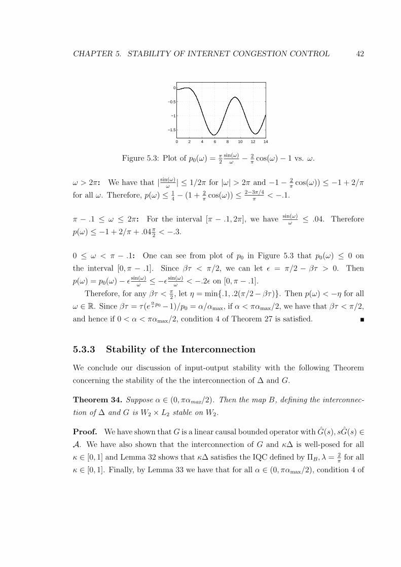
Define p0(ω) = p(ω) for βτ = π/2. The plot of p0(ω) = π2
sin(ω)ω
− 2π
cos(ω)−1 is given
in Figure 5.3. As one can see, the function is non-positive near the origin. In fact,
for any βτ < π/2, there exists an η > 0 such that p(ω) < −η for all ω. To see this,
consider the following domains.
CHAPTER 5. STABILITY OF INTERNET CONGESTION CONTROL 42
0 2 4 6 8 10 12 14
−1.5
−1
−0.5
0
Figure 5.3: Plot of p0(ω) = π2
sin(ω)ω
− 2π
cos(ω)− 1 vs. ω.
ω > 2π: We have that | sin(ω)ω| ≤ 1/2π for |ω| > 2π and −1− 2
πcos(ω)) ≤ −1 + 2/π
for all ω. Therefore, p(ω) ≤ 14− (1 + 2
πcos(ω)) ≤ 2−3π/4
π< −.1.
π − .1 ≤ ω ≤ 2π: For the interval [π − .1, 2π], we have sin(ω)ω
≤ .04. Therefore
p(ω) ≤ −1 + 2/π + .04π2
< −.3.
0 ≤ ω < π − .1: One can see from plot of p0 in Figure 5.3 that p0(ω) ≤ 0 on
the interval [0, π − .1]. Since βτ < π/2, we can let ε = π/2 − βτ > 0. Then
p(ω) = p0(ω)− ε sin(ω)ω
≤ −ε sin(ω)ω
< −.2ε on [0, π − .1].
Therefore, for any βτ < π2, let η = min.1, .2(π/2− βτ). Then p(ω) < −η for all
ω ∈ R. Since βτ = τ(eατ
p0−1)/p0 = α/αmax, if α < παmax/2, we have that βτ < π/2,
and hence if 0 < α < παmax/2, condition 4 of Theorem 27 is satisfied.
5.3.3 Stability of the Interconnection
We conclude our discussion of input-output stability with the following Theorem
concerning the stability of the the interconnection of ∆ and G.
Theorem 34. Suppose α ∈ (0, παmax/2). Then the map B, defining the interconnec-
tion of ∆ and G is W2 × L2 stable on W2.
Proof. We have shown that G is a linear causal bounded operator with G(s), sG(s) ∈A. We have also shown that the interconnection of G and κ∆ is well-posed for all
κ ∈ [0, 1] and Lemma 32 shows that κ∆ satisfies the IQC defined by ΠB, λ = 2π
for all
κ ∈ [0, 1]. Finally, by Lemma 33 we have that for all α ∈ (0, παmax/2), condition 4 of

CHAPTER 5. STABILITY OF INTERNET CONGESTION CONTROL 43
Theorem 27 is satisfied. We can therefore use Theorem 27 to prove W2×L2 stability
on W2 of the interconnection for any α ∈ (0, παmax/2).
5.4 Asymptotic Stability
In this section, we show that W2 × L2 stability on W2 of the interconnection implies
asymptotic stability of the original formulation of the congestion control protocol.
Recall that the original solution map A is defined by the following.
z(t) = fc(z(t),−z(t− τ)) t ≥ 0 (5.6)
z(t) = x0(t) t ∈ [−τ, 0] (5.7)
The interconnection maps B and Bz, however, are defined by the following differ-
ential equation.
z(t) = fc(z(t), f(t)− z(t− τ)) t ≥ 0 (5.8)
z(t) = 0 t ≤ 0 (5.9)
In the previous section, we have proven W2 × L2 stability on W2 of the map B
where B represents a reformulation of the problem in the input-output framework. We
would like to show, however, that for some X ⊂ Cτ this result also implies asymptotic
stability on X of the solution map A, where A represents the original formulation of
the problem. This is done in the following Theorem.
Theorem 35. Suppose α ∈ (0, παmax/2). Then the delay-differential equation (5.1)
describing the algorithm proposed by Paganini et al. [29] is asymptotically stable on
X = x : x ∈ W2 ∩ Cτ , x(t) ≥ −p0, x(−τ) > −p0.
Proof. We have already shown W2 × L2 stability on W2 of the map B. Let
x0 ∈ X be an arbitrary initial condition. Theorem 121 in the Appendix states that
for any initial condition x0 ∈ X, there exists some f ∈ W2 and T > 0 such that
A(x0, t) = Bz(f, t + T ) for all t ≥ 0. Let (y, u) = B(f), then y ∈ W2. Furthermore,

CHAPTER 5. STABILITY OF INTERNET CONGESTION CONTROL 44
recall Bzf = ∆zy where Bz is the map to internal variable z. By Lemma 30, if
y ∈ W2, then limt→∞ ∆z(y, t) = 0. Therefore, limt→∞ A(x0, t) = limt→∞ Bz(f, t+T ) =
limt→∞ ∆z(y, t + T ) = 0.
5.5 Implementation
To implement the proposed algorithm in the Internet framework, the window size
can be adjusted to deliver the required packet rate as given by equation (4.1). In
implementation, the delay is unlikely to be known. In this case, a bound on the
expected delay size can be used. Overestimation of the delay will result in an increased
stability margin.
Modification of the link can take many forms. Price information from the link
must be fed back to the source. Since queues themselves integrate excess rate, price
of a congested resource can be computed directly using the queueing delay. How-
ever, this approach results in non-empty equilibrium queues and the possibility of
unmodeled dynamics due to variable queueing delays. If a link instead uses a virtual
capacity to avoid non-empty equilibrium queues, then explicit integration of incoming
packets would be required and another mechanism must be used to feed back price
information. An example of direct feedback of price information using packet mark-
ing is given by ECN. In one of the proposed implementations, packets are randomly
marked at each link with probability 1−φ−pj(t) for some fixed φ > 1. Thus, assuming
no duplications, if ν is the percentage of marked packets received at the source, then
the aggregate price can be measured as qi(t) = − log(1−ν)log(φ)
. This variant is known as
random exponential marking.
5.6 Conclusion
To summarize, for the case of a single source with a single link, we have demonstrated
both input-output and asymptotic stability. We have used a generalized passiv-
ity framework to decompose a difficult nonlinear, discontinuous, infinite-dimensional
problem into separate linear, infinite-dimensional and nonlinear, finite-dimensional
CHAPTER 5. STABILITY OF INTERNET CONGESTION CONTROL 45
subproblems, each of which is amenable to existing analysis techniques. A key fea-
ture of the analysis of the nonlinear subsystem was the existence of a sector bound
on the nonlinearity.
In addition to the case of a single source with a single link, the result presented
in this chapter applies directly to the case of multiple sources with identical fixed
delay. The proof may also be easily adapted to alternate implementations of the
proposed linearized protocols so long as they admit a similar sector bound on the
nonlinearity. Although we would like to have proven a result in the case of multiple
heterogeneous delays and arbitrary topology, we have as yet not been able to construct
an appropriate sector bound. The root of the problem seems to lie in the discontinuity
due to the projection used in the gradient projection algorithm.
Chapter 6
Sum-of-Squares and Convex
Optimization
6.1 Convexity and Tractability
Consider the following optimization problem for fi ∈ R[x] for i = 0 . . . nf .
max f0(x) :
fi(x) ≥ 0, i = 1, . . . , nf
The problem as formulated is clearly, in general, not convex. In fact, many NP -
hard problems can be formulated in this manner. However, if we define Y := x :
fi(x) ≥ 0, i = 1 . . . nf, then the problem can be recast as an equivalent convex
optimization problem as follows.
max γ :
f0(x)− γ ∈ PY
Although this reformulation is convex, we must conclude that it too is intractable,
46

CHAPTER 6. SUM-OF-SQUARES AND CONVEX OPTIMIZATION 47
unless we believe that P = NP . The point that we make with this section is that
convexity, by itself, is not a sufficient condition for tractability of a problem. What
we need in addition is an efficient linear test for membership in the set PY [x]. Con-
struction of such membership tests for various sets is the goal of Chapters 6, 7, and 8.
6.2 Sum-of-Squares Decomposition
Any polynomial, f ∈ R[x], of degree d and n variables can be expressed as the linear
combination of(
n+dd
)monomials.
f(x) =
(n+dd )∑
i=1
cixγi,1
1 · · · xγi,nn γi,j ∈ Z+ (6.1)
The question of whether f ∈ P+, that is, f(x) ≥ 0 for all x ∈ Rn, is NP hard for
polynomials of degree 4 or more. Thus there is unlikely to exist a computationally
tractable set membership test for P+ unless P = NP . However, there may exist some
convex cone Σ ⊂ P+ for which the set membership test is computationally tractable.
One such cone is defined as follows.
Definition 36. A polynomial s ∈ R[x] satisfies s ∈ Σs if it can be represented in the
following form for some finite set of polynomials gi ∈ R[x], i = 1 . . . m.
s(x) =m∑
i=1
gi(x)2
An element s ∈ Σs is referred to as a sum-of-squares polynomial. The set Σds is
defined as the elements of Σs of degree d or less.
Lemma 37. Σds ⊂ P+
In [33], it was shown that the set membership test f ∈ Σs is computationally
tractable.
CHAPTER 6. SUM-OF-SQUARES AND CONVEX OPTIMIZATION 48
Lemma 38. A degree 2d polynomial f ∈ R[x] satisfies f ∈ Σs if and only if there
exists some matrix Q ∈ Snz where nz =(
n+dd
), such that Q ≥ 0 and
f(x) = Zd[x]T QZd[x].
The equality constraint in Lemma 38 is affine in the monomial coefficients of f .
Therefore, set membership in Σs can be tested using semidefinite programming. The
question of how well Σs represents P+ has been a topic on ongoing research for some
time. It was conclusively shown through use of the Motzkin polynomial that in gen-
eral Σs 6= P+. However, if we define Σr to be the convex cone of sums of squares of
quotients of polynomials, then Artin showed that Σr = P+. Not surprisingly, how-
ever, there is no tractable set membership test for Σr. As an interesting corollary of
this result, it was shown that f ∈ P+ if and only if there exists some g ∈ Σs such that
fg ∈ Σs. This does not constitute a tractable set membership test, unfortunately,
since no bound is given on the degree of g. In addition, the introduction of the auxil-
iary variable g destroys the convexity of the constraint since the resulting feasibility
problem is bilinear. Building on this work, however, Reznick showed that if f ∈ P+,
then there exists some d ∈ Z+ such that (xT x)d(f(x) + 1) ∈ Σs. This result provides
a test for membership of f in the interior of P+, but not a tractable one, as there are,
in general, still no bounds on d. What the result of Reznick does provide, however,
is a sequence of tractable tests for membership in the interior of P+, indexed by the
integer d.
6.3 Positivstellensatz Results
Membership in the cone PK is harder to approximate than P+. Consider a region
Kf of the following form for fi ∈ R[x], i = 1, . . . , nK .
Kf := x ∈ Rn : fi(x) ≥ 0, i = 1, . . . , nK.
Then f0 ∈ PKf if and only if the following set is empty.
CHAPTER 6. SUM-OF-SQUARES AND CONVEX OPTIMIZATION 49
K∗f := x ∈ Rn : −f0(x) ≥ 0, f0(x) 6= 0, fi(x) ≥ 0, i = 1, . . . , nK
A condition for emptiness of the set K∗f comes from the following simplified Posi-
tivstellensatz result from Stengle [44].
Theorem 39. Let Kf be given as above and let I denote the set of subsets of
0, . . . , nK. Then −f0 ∈ PKf if and only if there exist s ∈ Σs, sJ ∈ Σs, J ∈ I
and k ∈ Z+ such that
s(x) +∑J∈I
sJ(x)∏i∈J
fi(x) + f0(x)2k = 0
The Positivstellensatz condition given by Stengle is not tractable, due to the
introduction of bilinear terms sJf0 and since no degree bound exists on either k
or the degrees of the sJ . In the work by Schmudgen, the convexity problem was
addressed by considering the case when Kf is compact. This result can be stated as
follows.
Theorem 40. Let I be the set of subsets of 1, . . . , nK and suppose Kf , as defined
above, is compact. Suppose f lies in the interior of PKf . Then there exist sJ ∈ Σs
for J ∈ I, such that the following holds.
f(x)−∑
J∈I
sJ(x)∏i∈J
fi(x) ∈ Σs
Theorem 40 differs from Stengle’s result by essentially allowing us to set sJ =
0 when 0 6∈ J . This means that the resulting constraint is convex. However,
Schmudgen’s result still does not constitute a tractable condition since there exist
no bounds on the degrees of the sJ . The theorem does, however, suggest a method
for constructing a sequence of sufficient conditions for membership in the set PKf by
considering elements of Σs of bounded degree.
Definition 41. For a given degree bound, d, and compact semi-algebraic set, Kf ,
of the form given above and I as defined above, we define the convex cone ΛKf
d of

CHAPTER 6. SUM-OF-SQUARES AND CONVEX OPTIMIZATION 50
functions f ∈ R[x] such that there exist functions sJ ∈ Σds for J ∈ I, of degree d or
less, such that the following holds.
f(x)−∑
J∈I
sJ(x)∏i∈J
fi(x) ∈ Σs
Lemma 42. For any d ∈ Z+ and any Kf , ΛKf
d ⊂ PKf
Testing membership in ΛKf
d is a tractable problem for any fixed d and Kf and thus
provides a tractable sufficiency test for membership in PKf . However, the complexity
of the test scales poorly in nk. This problem was addressed to some extent by the
work of Putinar [39], which showed that under certain additional restrictions on the
set Kf , that we can assume that sJ = 0 for all J except J = 1, . . . , nK . This theorem
is stated as follows.
Definition 43. We say that fi ∈ R[x] for i = 1, . . . , nK define a P-compact set
Kf , if there exist h ∈ R[x] and si ∈ Σs for i = 0, . . . , nK such that the level set
x ∈ Rn : h(x) ≥ 0 is compact and such that the following holds.
h(x)−nK∑i=1
si(x)fi(x) ∈ Σs
The condition that a region be P-compact may be difficult to verify. However,
some important special cases include:
• Any region Kf such that all the fi are linear.
• Any region Kf defined by fi such that there exists some i for which the level
set x : fi(x) ≥ 0 is compact.
Thus any compact region can be made P-compact by inclusion of a redundant
constraint of the form fnK+1 := β − xT x for sufficiently large β. However, for such
an inclusion, we must have some explicit bound for the size of the original region.
Theorem 44. Suppose Kf , as defined above, is P-compact. Suppose f lies in the
interior of PKf . Then there exist si ∈ Σs for i = 1, . . . , nK, such that the following

CHAPTER 6. SUM-OF-SQUARES AND CONVEX OPTIMIZATION 51
holds.
f(x)−nK∑i=1
si(x)fi(x) ∈ Σs
Theorem 44 is similar to the Positivstellensatz result of Schmudgen in that it does
not represent a tractable test for membership in PKf since no bounds exist for the
degree of the si. However, Putinar’s Positivestellensatz provides a basis for a less
computationally intensive sequence of tractable sufficient conditions.
Definition 45. For a given degree bound, d, and semi-algebraic set, Kf , of the form
given above, we define the convex cone ΥKf
d of functions f ∈ R[x] such that there
exist si ∈ Σds for i = 1, . . . , nK, such that the following holds.
f(x)−nK∑i=1
si(x)fi(x) ∈ Σs
Lemma 46. For any d ∈ Z+ and any Kf , ΥKf
d ⊂ PKf
Membership in the set ΥKf
d is a tractable problem for any d ∈ Z+ and Kf and
can be tested using semidefinite programming. Moreover, for any fixed d, the test
associated with ΥKf
d is less computationally difficult than that associated with ΛKf
d ,
especially for large values of nK . However, such statements should be taken with a
grain of salt, since, for a fixed d, ΛKf
d may well provide a better approximation of
PKf than ΥKf
d .
6.4 Applications
In this section, we demonstrate some applications of the techniques provided in Sec-
tions 6.2 and 6.3 to stability of nonlinear ordinary differential equations. Our concepts
of stability are the same as those defined for functional differential equations, albeit
with a state space defined in Rn as opposed to Cτ .
CHAPTER 6. SUM-OF-SQUARES AND CONVEX OPTIMIZATION 52
6.4.1 Stability of Ordinary Differential Equations
Consider a time-invariant ordinary differential equation of the following form.
x(t) = f(x(t))
Here x(t) ∈ Rn and f is a polynomial of degree m such that f(0) = 0.
Theorem 47. The system defined by the polynomial function f is globally stable if
there exists an α > 0 and a Lyapunov function, V (x), with continuous derivatives
such that V (0) = 0 and the following holds.
V (x) ≥ αxT x for all x ∈ Rn
∇V (x)T f(x) ≤ 0 for all x ∈ Rn
If, in addition, V (x)T f(x) ≤ −αxT x for all x ∈ Rn, then the system is globally
asymptotically stable.
By using the methods of the Section 6.2, we can pose the question of existence
of Lyapunov function proving global stability of the system as a convex feasibility
problem in the cone P+. Then, by approximating P+ by Σs, we can construct a
sequence of sufficient conditions, of increasing accuracy, indexed by integers d, n ≥ 0,
which can be expressed as semidefinite programs.
Theorem 48. The origin is globally asymptotically stable if there exists a V ∈ R[x],
of degree d, and an α > 0, such that the following conditions hold.
V (x)− αxT x ∈ Σs
−(∇V (x)T f(x) + αxT x) ∈ Σs
6.4.2 Local Stability and Parametric Uncertainty
Consider a time-invariant ordinary differential equation of the following form.
x(t) = f(p, x(t))

CHAPTER 6. SUM-OF-SQUARES AND CONVEX OPTIMIZATION 53
Here x(t) ∈ Rn, p ∈ Rdp and f is a polynomial of degree m such that f(p, 0) = 0 for
all p ∈ K ⊂ Rdp . We first give a local, parameter-dependent version of Theorem 47.
Theorem 49. Let Ω ⊂ Rn contain an open neighborhood of the origin and f ∈ R[p, x]
satisfy f(p, 0) = 0 for all p ∈ K. Suppose there exists an α > 0 and a Lyapunov
function, V (p, x), with continuous derivatives such that V (p, 0) = 0 for p ∈ K and
the following holds.
V (p, x) ≥ αxT x for all x ∈ Ω, p ∈ K
∇xV (p, x)T f(p, x) ≤ 0 for all x ∈ Ω, p ∈ K
Then, for any p ∈ K, the system defined by f is stable on some open neighborhood of
the origin. If, in addition, V (p, x)T f(p, x) ≤ −αxT x for all x ∈ Ω and p ∈ K, then
for any p ∈ K, the system is asymptotically stable on some open neighborhood of the
origin.
Suppose the sets Ω and K are given by Kx and Kp, respectively, where Kx :=
x ∈ Rn : gi(x) ≥ 0, i = 1, . . . , ng for gi ∈ R[x] and Kp := p ∈ Rdp : hi(x) ≥ 0, i =
1, . . . , nh for hi ∈ R[x]. Now let the set K× be the intersection of the sets Kx and
Kp in the product space Rn+dp , defined as follows.
K× := (p, x) ∈ Rn+dp : p ∈ Kp, x ∈ Kx
By using the methods of the Sections 6.2 and 6.3, we can pose the stability con-
ditions associated with Theorem 49 as a convex feasibility problem in the convex
cone PK× . Then, for a given d ∈ Z+, by approximating PK× by ΛK×d or Υ
K×d , we
can construct a sequence of sufficient conditions, of increasing accuracy, indexed by
integers d, r ≥ 0, which can be expressed as semidefinite programs.
Theorem 50. Let f be a polynomial such that f(p, 0) = 0 for all p ∈ Kp and Kx
contain an open neighborhood of the origin. Suppose there exists a V ∈ R[p, x], of

CHAPTER 6. SUM-OF-SQUARES AND CONVEX OPTIMIZATION 54
degree r, and an α > 0 such that the following conditions hold.
V (p, x)− αxT x ∈ ΥK×d
−(∇xV (p, x)T f(p, x) + αxT x) ∈ ΥK×d
Then, for any p ∈ Kp, the origin is asymptotically stable in some open region about
the origin.
6.5 The SOS Representation of Matrix Functions
The previous sections discussed tractable tests for membership in the convex cones
P+ and PK of non-negativity scalar polynomials. In this section, we present an
extension of these results to the convex cones S+n and SK
n of non-negative matrices
of polynomials. A simple test for M ∈ S+n or M ∈ SK
n can be performed through the
introduction of n auxiliary variables.
Lemma 51. For M ∈ Sn[x], let fM ∈ R[x, y] be defined as f(x, y) := yT M(x)y.
1. M ∈ S+n if and only if fM ∈ P+.
2. M ∈ SKn if and only if fM ∈ PK′
, where K ′ := (x, y) : x ∈ K.
Thus, we can determine whether M ∈ S+n by testing whether fM ∈ P+ using the
techniques discussed in the previous section. The problem with this approach is that
the size of the resulting semidefinite program scales very poorly in the dimension of
M . This is due to the introduction of the auxiliary variables y. Instead, we will
consider the following direct approximation to the cone S+n .
Definition 52. M ∈ Sn[x] satisfies M ∈ Σs if it can be represented in the following
form for some finite set of polynomial matrices Gi ∈ Rn×n[x], i = 1, . . . ,m.
M(x) =m∑
i=1
Gi(x)T Gi(x)

CHAPTER 6. SUM-OF-SQUARES AND CONVEX OPTIMIZATION 55
An element M ∈ Σs is referred to as a sum-of-squares matrix function. Fur-
thermore, define Σds to be elements of Σs of degree d or less.
We now provide a tractable test for membership in Σs.
Lemma 53. Suppose M ∈ Sn2d[x] for x ∈ Rn2. M ∈ Σs if and only if there exists
some matrix Q ∈ Snz ·n, where nz =(
n2+dd
)such that Q ≥ 0 and the following holds.
M(x) =(Zn
d [x])T
QZnd [x]
See Appendix B for Proof.
The complexity of the membership test associated with Lemma 53 is considerably
lower than that associated with Lemma 51. Specifically, the variables associated with
the first test are of order n(
n2+dd
)as opposed to order
(n+n2+d+1
d+1
). Furthermore, the
use of the test associated with Lemma 53 does not increase the conservatively, as
evidenced by the following lemma.
Lemma 54. M(x) ∈ Σs if and only if yT M(x)y ∈ Σs.
See Appendix B for Proof.
As for Σs and P+, the question of how well Σs approximates S+n is an open
question. However, in the case of a single variable, we have the following result due
to Choi et al. [5].
Lemma 55. For x ∈ R, M ∈ Sn[x], the following are equivalent
• M ∈ Σs
• M ∈ S+n .
Lemma 55 will find considerable application in Chapter 7.

CHAPTER 6. SUM-OF-SQUARES AND CONVEX OPTIMIZATION 56
6.6 Positivstellensatz Results for Matrix Functions
In this section, we consider membership in the set SKfn for some semi-algebraic set
Kf , defined by polynomials fi ∈ R[x] as follows.
Kf := x : fi(x) ≥ 0, i = 1 . . . nf
Scherer and Hol [43] have proven the following generalization of Putinar’s Posi-
tivstellensatz.
Theorem 56. Suppose that Kf is P-compact and M ∈ SKfn . Then there exist η > 0
and Si ∈ Σs for i = 1, . . . , nf such that the following holds.
M(x)−nf∑i=1
fi(x)Si(x)− εI ∈ Σs
Theorem 56 does not represent a tractable test for SKfn , since no degree bounds are
given on the Si. However, the result does suggest a sequence of sufficient conditions,
indexed by d ∈ Z+, and defined as follows.
Definition 57. We say that M ∈ ΥKf
n,d if there exist η > 0 and Si ∈ Σds for i =
1, . . . , nf such that the following holds.
M(x)−nf∑i=1
fi(x)Si(x) ∈ Σs
Lemma 58. For any d ≥ 0 and Kf , ΥKf
n,d ⊂ SKfn .
Therefore, for any d ≥ 0, we can construct a tractable test for membership in the
convex cone ΥKf
n,d, expressible as a semidefinite program. Furthermore, as d increases,
ΥKf
n,d will constitute a better approximation for SKfn .

CHAPTER 6. SUM-OF-SQUARES AND CONVEX OPTIMIZATION 57
6.6.1 Linear ODEs with Parametric Uncertainty
The most common application for the sum-of-squares matrix representation is the case
of a linear finite-dimensional system which contains uncertainty. Consider a system
of ordinary differential equations of the following form where A : Rny → Rn×n.
x(t) = A(y)x(t) y ∈ G (6.2)
The following is a standard result in analysis of LTI systems.
Theorem 59. The system defined by Equation 6.2 is globally asymptotically stable
for all y ∈ G if and only if there exists a matrix function P : G → Sn such that the
following conditions hold.
P (y)− I ∈ SGn
−(A(y)T P (y) + P (y)A(y) + I) ∈ SGn
Now suppose that G is a semi-algebraic set defined by polynomials ging
i=1. Then
for integer d ≥ 0, we can approximate the conditions 59 using the following.
Theorem 60. The system defined by Equation 6.2 is globally asymptotically stable
for all y ∈ G if there exists a matrix of polynomials P ∈ Sn[y] such that the following
conditions hold.
P (y)− I ∈ ΥGn,d
−(A(y)T P (y) + P (y)A(y) + I) ∈ ΥGn,d
The conditions of Theorem 60 can be expressed as a semidefinite program.

CHAPTER 6. SUM-OF-SQUARES AND CONVEX OPTIMIZATION 58
6.7 Conclusion
This chapter has detailed a method for expressing may difficult problems in control
as convex optimization problems. These optimization problems are, in general, not
tractable due to the lack of an efficient membership test for the convex cone P+.
However, we have shown that by approximating P+ by Σs, one can construct tractable
approximations. The techniques and concepts of this chapter will play an integral role
as we seek to generalize the ODE applications presented in subsections 6.4.1, 6.4.2,
and 6.6.1 to differential equations which contain delay.

Chapter 7
Stability of Linear Time-Delay
Systems
7.1 Introduction
The study of stability of systems of differential equations which contain delays has
been an active area of research for some time. A complete summary of the results
in this field is beyond the scope of this paper. However, an overview of these re-
sults can be obtained from various survey papers and books on the subject, see for
example [13, 14, 19, 28]. The previous results on this subject can be grouped into
analysis either in the frequency-domain or in the time-domain. Frequency-domain
techniques apply only to linear systems and typically attempt to determine whether
all roots of the characteristic equation of the system lie in the left half-plane. Time-
domain techniques generally use Lyapunov-based analysis, an approach which was
extended to infinite dimensional systems by Krasovskii in [20]. Stability results in
this area are grouped into delay-dependent and delay-independent conditions. If a
delay-dependent condition holds, then stability is guaranteed for a specific value or
range of values of the delay. If a delay-independent condition holds, then the system
is stable for all possible values of the delay. A particularly interesting result on the
linear delay-independent case appears in [3].
In this chapter, we show how to compute solutions to an operator-theoretic version
59
CHAPTER 7. STABILITY OF LINEAR TIME-DELAY SYSTEMS 60
of the Lyapunov inequality using semidefinite programming. This inequality, defined
by the derivative of the complete quadratic functional, can be posed as a convex
feasibility problem over certain infinite-dimensional convex cones defined by positive
operators on certain subspaces of Cτ . Our result is expressed as a nested sequence
of sufficient conditions which are of increasing accuracy and can be tested using
semidefinite programming. Our approach is based on parameterizing the convex
cones mentioned above using polynomial functions of bounded degree.
7.2 Positive Operators
In this section, we present the convex cones of positive multiplier and integral oper-
ators which define the complete quadratic functional and some its derivative forms.
We then use polynomials of bounded degree to parametrization certain convex sub-
sets of these cones in terms of positive semidefinite matrices. These results will allow
us to express the Lyapunov stability conditions in terms of semidefinite programming
problems. To begin, consider the complete quadratic functional.
V (x) = x(0)T Px(0) + 2
∫ 0
−τ
x(0)T Q(θ)x(θ)dθ
+
∫ 0
−τ
x(θ)T S(θ)x(θ)dθ +
∫ 0
−τ
∫ 0
−τ
x(θ)T R(θ, ω)x(ω)dθdω
We can associate with V and ε > 0 an operator A : Cτ → Cτ such that V (x) = 〈x,Ax〉,where A is defined as follows.
(Ay)(θ) =
[P − εI Q(θ)
Q(θ)T S(θ)
]y(θ) +
∫ 0
−τ
[0 0
0 R(θ, ω)
]y(ω)dω
= (A1y)(θ) + (A2y)(θ),
The operator A is a combination of multiplier operator A1 and integral operator
A2. The complete quadratic functional, V satisfies the positivity condition of the
stability theorem with u(φ(0)) = εφ(0)2 if the integral operator, A2, is positive on Cτ
CHAPTER 7. STABILITY OF LINEAR TIME-DELAY SYSTEMS 61
and there exists some ε > 0 such that the multiplication operator, A1, is positive on
the subspace X ⊂ Cτ where
X := x ∈ Cτ | , x =
[x1
x2
]and x1(θ) = x2(0) for all θ.
We now define the specific sets of operators which define the complete quadratic
functional and its derivative forms.
Definition 61. For a matrix-valued function M : R → Sn, we denote by AM the
multiplication operator such that
(AMx)(θ) = M(θ)x(θ)
Definition 62. For a matrix-valued function R : R×R→ Rn×n such that R(θ, ω) =
R(ω, θ)T , we denote by BR the integral operator such that
(BRx)(θ) =
∫ 0
−τ
R(θ, ω)x(ω)dω
Definition 63. For a continuous matrix-valued function M , we say M ∈ H+1 if
〈x,AMx〉 ≥ 0 for all x ∈ X.
Definition 64. For a continuous matrix-valued function R : R × R → Rn×n such
that R(θ, ω) = R(ω, θ)T , we say R ∈ H+2 if 〈x,BRx〉 ≥ 0 for all x ∈ Cτ .
Definition 65. For a piecewise-continuous matrix-valued function M , we say M ∈H+
1 if 〈x,AMx〉 ≥ 0 for all x ∈ X.
Definition 66. For a piecewise-continuous matrix-valued function R : R×R→ Rn×n
such that R(θ, ω) = R(ω, θ)T , we say R ∈ H+2 if 〈x,BRx〉 ≥ 0 for all x ∈ Cτ .
Definition 67. For a continuous matrix-valued function M , we say M ∈ H+3 if
CHAPTER 7. STABILITY OF LINEAR TIME-DELAY SYSTEMS 62
〈x,AMx〉 ≥ 0 for all x ∈ X3, where
X3 := x ∈ Cτ | , x =[xT
1 xT2 xT
3
]T
and x1(θ) = x3(0) and
x2(θ) = x3(−τ) for all θ.
Definition 68. For a piecewise-continuous matrix-valued function M , we say M ∈H+
3 if 〈x,AMx〉 ≥ 0 for all x ∈ X3, where
X3 :=
x ∈ Cτ | , x =[xT
1 . . . xTK+2
]T
and
xi(θ) = xK+2(−τi−1) for all θ, i = 1, . . . , K + 1
.
7.2.1 Multiplier Operators and Spacing Functions
In this subsection, we consider the convex cones H+1 and H+
3 which define positive
multiplication operators on X1 and X3 respectively. We use the following theorem.
Theorem 69. Suppose M : R → S2n is a continuous matrix-valued function. Then
the following are equivalent
1. There exists some ε > 0 such that the following holds for all x ∈ Cτ .
∫ 0
−τ
[x(0)
x(θ)
]T
M(θ)
[x(0)
x(θ)
]dθ ≥ ε‖x‖2
2
2. There exists some ε′ > 0 and some continuous matrix-valued function T : R→Sn such that the following holds.
∫ 0
−τ
T (θ)dθ = 0
M(θ) +
[T (θ) 0
0 −ε′I
]≥ 0 for all θ ∈ [−τ, 0]
See Appendix D for Proof.

CHAPTER 7. STABILITY OF LINEAR TIME-DELAY SYSTEMS 63
Definition 70. Given n and τ , we refer to any piecewise-continuous matrix-valued
function T : R → Rn such that∫ 0
−τT (θ)dθ = 0 as a spacing function, denoted
T ∈ Ω.
This theorem states that any element of H+1 which satisfies a certain additional
positivity condition can be represented by the combination of a positive semidefinite
matrix-valued function and a spacing function. This allows us to search for elements
of H+1 by simultaneously searching over the set of positive semidefinite matrix-valued
functions and the set of spacing functions. For any d ∈ Z+, the following gives a
tractable condition for membership in H+1 .
Definition 71. Given n and τ , define Ωdp to be the set of functions T ∈ Sn
d [θ] such
that the following holds. ∫ 0
−τ
T (θ)dθ = 0
Definition 72. For a given d ≥ 0, M ∈ S2n[θ] satisfies M ∈ Gd1 if there exists a
T ∈ Ωdp such that
M(θ) +
[T (θ) 0
0 0
]∈ P+.
Membership in the convex cone Gd1 can be implemented as a semidefinite pro-
gramming constraint by noting that the constraint that a polynomial integrate to 0
is affine in the coefficients and that for the single variable case, Σs = P+. We now
consider H+3 . We can use a simple extension of the previous theorem.
Lemma 73. Let M : R → S3n be a continuous matrix-valued function. Then the
following are equivalent.
1. There exists an ε > 0 such that the following holds for all x ∈ Cτ .
∫ 0
−τ
x(0)
x(−τ)
x(θ)
T
M(θ)
x(0)
x(−τ)
x(θ)
≥ ε‖x‖2
2

CHAPTER 7. STABILITY OF LINEAR TIME-DELAY SYSTEMS 64
2. There exists some ε′ > 0 and a continuous matrix-valued function T : R→ S2n
such that the following holds.
∫ 0
−τ
T (θ)dθ = 0
M(θ) +
[T (θ) 0
0 −ε′I
]≥ 0 for all θ ∈ [−τ, 0]
See Appendix D for Proof.
Definition 74. For a given d ≥ 0, M ∈ S3n[θ] satisfies M ∈ Gd3 if there exists a
T ∈ S2n[θ] such that T ∈ Ωdp and
M(θ) +
[T (θ) 0
0 0
]∈ P+.
Similar to Theorem 69, Lemma 73 allows us to use Gd3 ⊂ H+
3 to replace M ∈ H+3
with a semidefinite programming constraint.
Piecewise-Continuous Spacing Functions
We now consider the sets H+1 and H+
3 of piecewise continuous functions which define
positive multiplication operators on X1 and X3 respectively. The following lemma is
a generalization of Theorem 69.
Lemma 75. Suppose Si : R → S2n, i = 1, . . . , K are continuous symmetric matrix-
valued functions with domains [−τi,−τi−1] where τi > τi−1 for i = 1, . . . , K and
τ0 = 0. Then the following are equivalent.
1. There exists an ε > 0 such that the following holds for all x ∈ CτK.
K∑i=1
∫ −τi−1
−τi
[x(0)
x(θ)
]T
Si(θ)
[x(0)
x(θ)
]dθ ≥ ε‖x‖2
2

CHAPTER 7. STABILITY OF LINEAR TIME-DELAY SYSTEMS 65
2. There exists an ε′ > 0 and continuous symmetric matrix valued functions, Ti :
R→ Sn, such that
Si(θ) +
[Ti(θ) 0
0 −ε′I
]≥ 0 for θ ∈ [−τi,−τi−1], i = 1, . . . , K and
K∑i=1
∫ −τi−1
−τi
Ti(θ) = 0.
See Appendix D for Proof.
Lemma 75 allows us to represent the constrain S ∈ H+1 by considering a piecewise-
continuous function S to be defined by S(θ) := Si(θ) for θ ∈ [−τi,−τi−1].
Definition 76. Given n and τ , define Ωdp to be the set of piecewise-continuous func-
tions T : R → Sn such that T (θ) = Ti(θ) for Ti ∈ Snd [θ] and θ ∈ [−τi,−τi−1] where
i = 1, . . . , K and such thatK∑
i=1
∫ −τi−1
−τi
Ti(θ) = 0.
Definition 77. For a given d ≥ 0, we say that M : R → S2n satisfies M ∈ Gd1 if
there exists Mi ∈ S2nd [θ] such that M(θ) = Mi(θ) for θ ∈ [−τi,−τi−1] and there exists
a T ∈ Ωdp, defined by Ti ∈ Sn
d [θ] on the interval [−τi,−τi−1], and such that
Mi(θ) +
[Ti(θ) 0
0 0
]∈ P+ i = 1, . . . , K.
Similar to Theorem 69, Lemma 75 allows us to use Gd1 ⊂ H+
1 to replace M ∈ H+1
with a semidefinite programming constraint. Now for H+3 , we have the following
lemma.
Lemma 78. Suppose Si : R → Sn(K+2) are continuous matrix valued functions with
domains [−τi,−τi−1] for i = 1, . . . , K where τi > τi−1 for i = 1, . . . , K and τ0 = 0.
Then the following are equivalent.
CHAPTER 7. STABILITY OF LINEAR TIME-DELAY SYSTEMS 66
1. There exists an ε > 0 such that the following holds for all x ∈ CτK.
K∑i=1
∫ −τi−1
−τi
x(−τ0)...
x(−τK)
x(θ)
T
Si(θ)
x(−τ0)...
x(−τK)
x(θ)
dθ ≥ ε‖x‖22
2. There exists an ε′ > 0 and continuous matrix valued functions Ti : R→ Sn(K+1)
such that
Si(θ) +
[Ti(θ) 0
0 −ε′I
]≥ 0 for θ ∈ [−τi,−τi−1], i = 1, . . . , K and
K∑i=1
∫ −τi−1
−τi
Ti(θ) = 0.
See Appendix D for Proof.
Definition 79. For a given d ≥ 0, we say that M : R → Sn(K+2) satisfies M ∈ Gd3
if there exist Mi ∈ Sn(K+2)d [θ] such that M(θ) = Mi(θ) on [−τi,−τi−1] and Ti ∈
Sn(K+1)d [θ] such that T (θ) = Ti(θ) on [−τi,−τi−1] implies T ∈ Ωd
p and such that
Mi(θ) +
[Ti(θ) 0
0 0
]∈ P+ i = 1, . . . , K.
Similar to Theorem 69, Lemma 78 allows us to use Gd3 ⊂ H+
3 to replace M ∈ H+3
with a semidefinite programming constraint.
Parameter-Dependent Spacing Functions
In this subsection, we consider the case which arises when the dynamics of the system
depend on some uncertain time-invariant vector of parameters.

CHAPTER 7. STABILITY OF LINEAR TIME-DELAY SYSTEMS 67
Lemma 80. For a given d ∈ Z+ and S ∈ S2nd [θ, y], suppose there exists some T ∈
Snd [θ, y] such that the following holds.
∫ 0
−τ
T (θ, y)dθ = 0
S(θ, y) +
[T (θ, y) 0
0 0
]∈ Σs
Then S(·, y) ∈ H+1 for all y ∈ Rp.
Now suppose we wish to impose the condition that S(·, y) ∈ H+1 for all y ∈ y :
pi(y) ≥ 0, i = 1, . . . , N for scalar polynomials pi.
Lemma 81. Suppose there exist functions Si such that Si(·, y) ∈ H+1 for i = 0, . . . , N
for all y and such that the following holds.
S(θ, y) = S0(θ, y) +N∑
i=1
pi(y)Si(θ, y),
Then S(·, y) ∈ H+1 for all y ∈ y : pi(y) ≥ 0, i = 1, . . . , N
The purpose of these lemmas is to show how our representation of H+1 can be used
to prove stability in the presence of parametric uncertainty. Clearly, these results
are motivated by the construction ΥKd presented in Chapter 6. The generalization
of Lemmas 80 and 81 to H+3 , H+
1 and H+3 is similar and therefore not explicitly
discussed.
7.2.2 Positive Finite-Rank Integral Operators
We now consider the set H+2 of continuous matrix-valued kernel functions which
define positive integral operators on Cτ . These operators are compact and satisfy the
following inequality for all x ∈ Cτ .
∫ 0
−τ
∫ 0
−τ
x(θ)T k(θ, ω)x(ω)dθdω ≥ 0
CHAPTER 7. STABILITY OF LINEAR TIME-DELAY SYSTEMS 68
Because Cτ is an infinite dimensional space, we cannot fully parameterize the
operators which are positive on this space using a finite-dimensional set of positive
semidefinite matrices. Instead, we will consider the subset of finite-rank operators.
Theorem 82. Let A be a compact Hermitian operator which is positive on Ym ⊂ Cτ ,
where
Yd := p ∈ Cτ : p is an n-dimensional vector of
univariate polynomials of degree d or less.
Then there exists a positive semidefinite matrix Q ∈ Sn×(d+1) such that
〈x,Ax〉 =
∫ 0
−τ
∫ 0
−τ
x(θ)T k(θ, ω)x(ω)dθdω ∀x ∈ Ym
k(θ, ω) :=
Zd[θ]. . .
Zd[θ]
T
Q
Zd[ω]. . .
Zd[ω]
= Znd (θ)T QZn
d (ω),
where recall Zd[θ] is the (d + 1)-dimensional vector of powers of θ of degree d or less.
Before proving the theorem, we quote the following lemma which follows directly
from the Spectral Theorem [50].
Lemma 83. Let eipi=1 be a basis for some finite dimensional subspace Y of an inner
product space Z. Let A be some compact Hermitian operator which is positive on Y .
Then there exists some K ≥ 0 such that the following holds for all x ∈ Y .
〈x,Ax〉 =
p∑i,j=1
Kij〈ei, x〉〈ej, x〉
Proof. Define ei to be the transpose of the ith row of Znd , then ein(d+1)
i=1 forms a
basis for the finite dimensional subspace Ym ⊂ Cτ . By Lemma 83, there exists some
CHAPTER 7. STABILITY OF LINEAR TIME-DELAY SYSTEMS 69
Q ≥ 0 such that the following holds where p = n(d + 1).
〈x,Ax〉 =
p∑i,j=1
Qij〈ei, x〉〈ej, x〉
=
∫ 0
−τ
∫ 0
−τ
p∑i,j=1
Qijei(θ)T x(θ)ej(ω)T x(ω)dθdω
=
∫ 0
−τ
∫ 0
−τ
x(θ)T
p∑i,j=1
(ei(θ)Qijej(ω)T
)x(ω)dθdω
=
∫ 0
−τ
∫ 0
−τ
x(θ)T Znd [θ]T QZn
d [ω]x(ω)dθdω
Definition 84. For a given integer d ≥ 0, we denote the set of compact Hermitian
operators which are positive on Yd by G2d2
This theorem shows how we can use semidefinite programming to represent the
subset G2d2 which consists of finite rank elements of the convex cone H+
2 with polyno-
mial eigenvectors of bounded degree. Naturally, as we increase the degree bound, d,
the rank of the operators in G2d2 will increase, as will the computational complexity
of the problem.
Piecewise-Continuous Positive Finite-Rank Operators
In this subsection, we consider the set H+2 of matrix-valued kernel functions which
are discontinuous only at points θ, ω = −τiK−1i=1 and which define positive integral
operators on Cτ . Although the results of the previous section can be applied directly,
the kernel functions defined in such a manner will necessarily be continuous since they
are constructed using a finite number of continuous functions. In order to allow for the
construction of operators defined by piecewise-continuous matrix valued functions, we
use the following lemma.
Lemma 85. Let M be a matrix valued function M : R2 → Sn which is discontinuous
only at points θ, ω = −τi for i = 1, . . . , K − 1 where the τi are increasing and τ0 = 0.
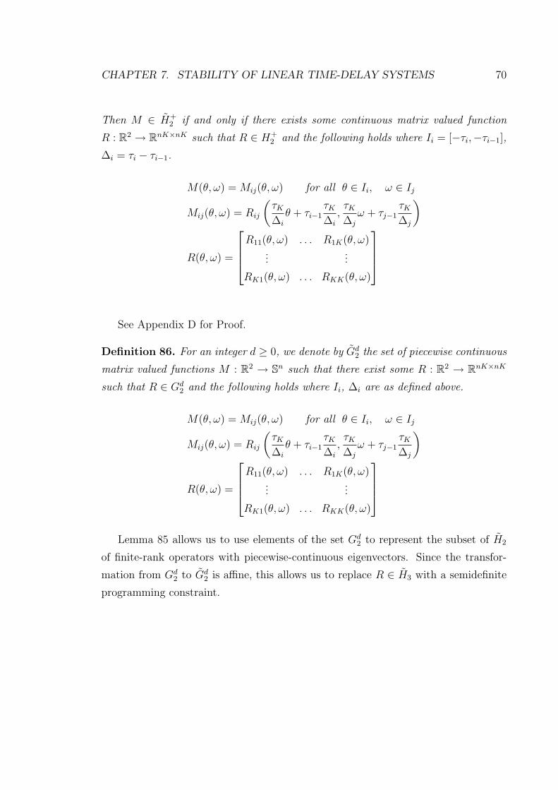
CHAPTER 7. STABILITY OF LINEAR TIME-DELAY SYSTEMS 70
Then M ∈ H+2 if and only if there exists some continuous matrix valued function
R : R2 → RnK×nK such that R ∈ H+2 and the following holds where Ii = [−τi,−τi−1],
∆i = τi − τi−1.
M(θ, ω) = Mij(θ, ω) for all θ ∈ Ii, ω ∈ Ij
Mij(θ, ω) = Rij
(τK
∆i
θ + τi−1τK
∆i
,τK
∆j
ω + τj−1τK
∆j
)
R(θ, ω) =
R11(θ, ω) . . . R1K(θ, ω)...
...
RK1(θ, ω) . . . RKK(θ, ω)
See Appendix D for Proof.
Definition 86. For an integer d ≥ 0, we denote by Gd2 the set of piecewise continuous
matrix valued functions M : R2 → Sn such that there exist some R : R2 → RnK×nK
such that R ∈ Gd2 and the following holds where Ii, ∆i are as defined above.
M(θ, ω) = Mij(θ, ω) for all θ ∈ Ii, ω ∈ Ij
Mij(θ, ω) = Rij
(τK
∆i
θ + τi−1τK
∆i
,τK
∆j
ω + τj−1τK
∆j
)
R(θ, ω) =
R11(θ, ω) . . . R1K(θ, ω)...
...
RK1(θ, ω) . . . RKK(θ, ω)
Lemma 85 allows us to use elements of the set Gd2 to represent the subset of H2
of finite-rank operators with piecewise-continuous eigenvectors. Since the transfor-
mation from Gd2 to Gd
2 is affine, this allows us to replace R ∈ H3 with a semidefinite
programming constraint.
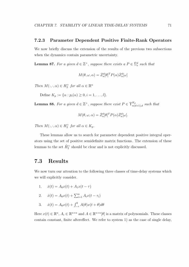
CHAPTER 7. STABILITY OF LINEAR TIME-DELAY SYSTEMS 71
7.2.3 Parameter Dependent Positive Finite-Rank Operators
We now briefly discuss the extension of the results of the previous two subsections
when the dynamics contain parametric uncertainty.
Lemma 87. For a given d ∈ Z+, suppose there exists a P ∈ Σds such that
M(θ, ω, α) = Zdn[θ]T P (α)Zd
n[ω]
Then M(·, ·, α) ∈ H+2 for all α ∈ Rn
Define Kp := α : pi(α) ≥ 0, i = 1, . . . , l.
Lemma 88. For a given d ∈ Z+, suppose there exist P ∈ ΥKp
n(d+1),d such that
M(θ, ω, α) = Zdn[θ]T P (α)Zd
n[ω].
Then M(·, ·, α) ∈ H+2 for all α ∈ Kp.
These lemmas allow us to search for parameter dependent positive integral oper-
ators using the set of positive semidefinite matrix functions. The extension of these
lemmas to the set H+2 should be clear and is not explicitly discussed.
7.3 Results
We now turn our attention to the following three classes of time-delay systems which
we will explicitly consider.
1. x(t) = A0x(t) + A1x(t− τ)
2. x(t) = A0x(t) +∑n
i=1 Aix(t− τi)
3. x(t) = A0x(t) +∫ 0
−τA(θ)x(t + θ)dθ
Here x(t) ∈ Rn, Ai ∈ Rn×n and A ∈ Rn×n[θ] is a matrix of polynomials. These classes
contain constant, finite aftereffect. We refer to system 1) as the case of single delay,
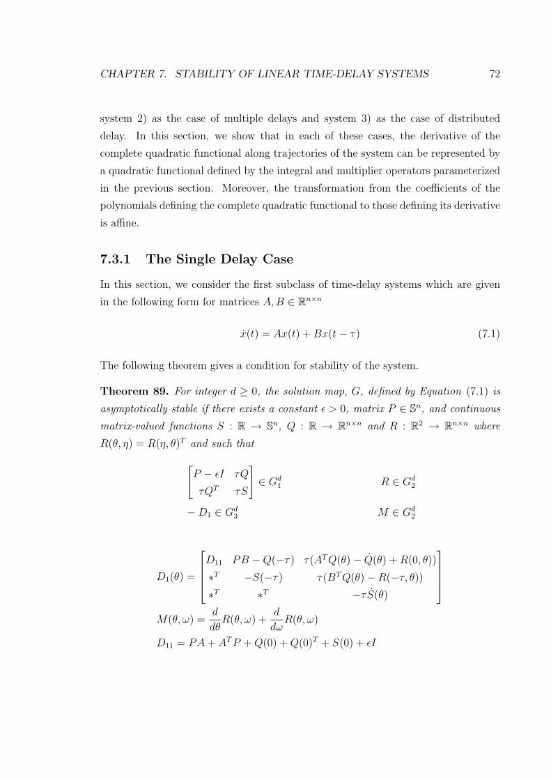
CHAPTER 7. STABILITY OF LINEAR TIME-DELAY SYSTEMS 72
system 2) as the case of multiple delays and system 3) as the case of distributed
delay. In this section, we show that in each of these cases, the derivative of the
complete quadratic functional along trajectories of the system can be represented by
a quadratic functional defined by the integral and multiplier operators parameterized
in the previous section. Moreover, the transformation from the coefficients of the
polynomials defining the complete quadratic functional to those defining its derivative
is affine.
7.3.1 The Single Delay Case
In this section, we consider the first subclass of time-delay systems which are given
in the following form for matrices A,B ∈ Rn×n
x(t) = Ax(t) + Bx(t− τ) (7.1)
The following theorem gives a condition for stability of the system.
Theorem 89. For integer d ≥ 0, the solution map, G, defined by Equation (7.1) is
asymptotically stable if there exists a constant ε > 0, matrix P ∈ Sn, and continuous
matrix-valued functions S : R → Sn, Q : R → Rn×n and R : R2 → Rn×n where
R(θ, η) = R(η, θ)T and such that
[P − εI τQ
τQT τS
]∈ Gd
1 R ∈ Gd2
−D1 ∈ Gd3 M ∈ Gd
2
D1(θ) =
D11 PB −Q(−τ) τ(AT Q(θ)− Q(θ) + R(0, θ))
∗T −S(−τ) τ(BT Q(θ)−R(−τ, θ))
∗T ∗T −τ S(θ)
M(θ, ω) =d
dθR(θ, ω) +
d
dωR(θ, ω)
D11 = PA + AT P + Q(0) + Q(0)T + S(0) + εI
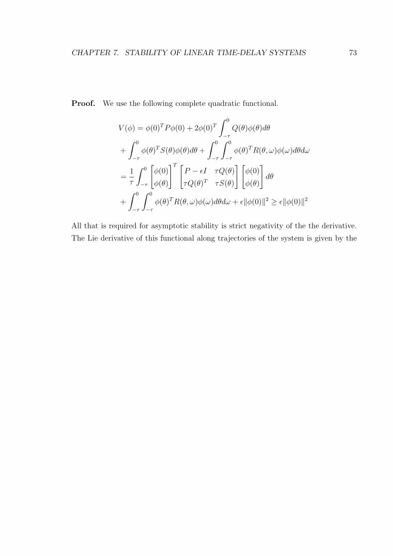
CHAPTER 7. STABILITY OF LINEAR TIME-DELAY SYSTEMS 73
Proof. We use the following complete quadratic functional.
V (φ) = φ(0)T Pφ(0) + 2φ(0)T
∫ 0
−τ
Q(θ)φ(θ)dθ
+
∫ 0
−τ
φ(θ)T S(θ)φ(θ)dθ +
∫ 0
−τ
∫ 0
−τ
φ(θ)T R(θ, ω)φ(ω)dθdω
=1
τ
∫ 0
−τ
[φ(0)
φ(θ)
]T [P − εI τQ(θ)
τQ(θ)T τS(θ)
][φ(0)
φ(θ)
]dθ
+
∫ 0
−τ
∫ 0
−τ
φ(θ)T R(θ, ω)φ(ω)dθdω + ε‖φ(0)‖2 ≥ ε‖φ(0)‖2
All that is required for asymptotic stability is strict negativity of the the derivative.
The Lie derivative of this functional along trajectories of the system is given by the
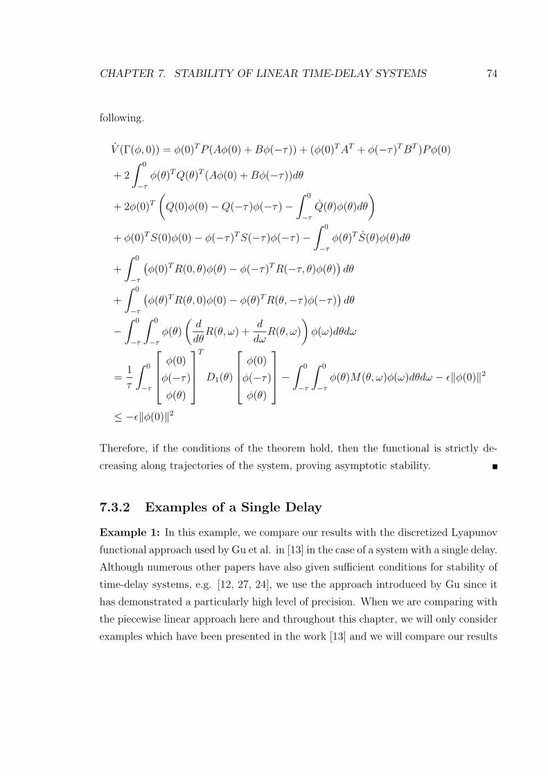
CHAPTER 7. STABILITY OF LINEAR TIME-DELAY SYSTEMS 74
following.
V (Γ(φ, 0)) = φ(0)T P (Aφ(0) + Bφ(−τ)) + (φ(0)T AT + φ(−τ)T BT )Pφ(0)
+ 2
∫ 0
−τ
φ(θ)T Q(θ)T (Aφ(0) + Bφ(−τ))dθ
+ 2φ(0)T
(Q(0)φ(0)−Q(−τ)φ(−τ)−
∫ 0
−τ
Q(θ)φ(θ)dθ
)
+ φ(0)T S(0)φ(0)− φ(−τ)T S(−τ)φ(−τ)−∫ 0
−τ
φ(θ)T S(θ)φ(θ)dθ
+
∫ 0
−τ
(φ(0)T R(0, θ)φ(θ)− φ(−τ)T R(−τ, θ)φ(θ)
)dθ
+
∫ 0
−τ
(φ(θ)T R(θ, 0)φ(0)− φ(θ)T R(θ,−τ)φ(−τ)
)dθ
−∫ 0
−τ
∫ 0
−τ
φ(θ)
(d
dθR(θ, ω) +
d
dωR(θ, ω)
)φ(ω)dθdω
=1
τ
∫ 0
−τ
φ(0)
φ(−τ)
φ(θ)
T
D1(θ)
φ(0)
φ(−τ)
φ(θ)
−
∫ 0
−τ
∫ 0
−τ
φ(θ)M(θ, ω)φ(ω)dθdω − ε‖φ(0)‖2
≤ −ε‖φ(0)‖2
Therefore, if the conditions of the theorem hold, then the functional is strictly de-
creasing along trajectories of the system, proving asymptotic stability.
7.3.2 Examples of a Single Delay
Example 1: In this example, we compare our results with the discretized Lyapunov
functional approach used by Gu et al. in [13] in the case of a system with a single delay.
Although numerous other papers have also given sufficient conditions for stability of
time-delay systems, e.g. [12, 27, 24], we use the approach introduced by Gu since it
has demonstrated a particularly high level of precision. When we are comparing with
the piecewise linear approach here and throughout this chapter, we will only consider
examples which have been presented in the work [13] and we will compare our results

CHAPTER 7. STABILITY OF LINEAR TIME-DELAY SYSTEMS 75
with the numbers that are cited therein. We use SOSTools [32] and SeDuMi [45]
for solution of all semidefinite programming problems. Now consider the following
system of delay differential equations.
x(t) =
[0 1
−2 0.1
]x(t) +
[0 0
1 0
]x(t− τ)
The problem is to estimate the range of τ for which the differential equation remains
stable. Using the method presented in this paper and by sweeping τ in increments of
.1, we estimate the range of stability to be an interval. We then use a bisection method
to find the minimum and maximum stable delay. Our results are also summarized in
Table 7.1 and are compared to the analytical limit and the results obtained in [13].
Our resultsd τmin τmax
1 .10017 1.62492 .10017 1.71723 .10017 1.71785
Analytic .10017 1.71785
Piecewise FunctionalN2 τmin τmax
1 .1006 1.42722 .1003 1.69213 .1003 1.7161
Table 7.1: τmax and τmin for discretization level N2 using the piecewise-linear Lya-punov functional and for degree d using our approach and compared to the analyticallimit
Clearly, the results for this test case illustrate a high rate of convergence to the
analytical limit. However, although the results presented here give reasonable esti-
mates for the interval of stability, they do not prove stability over any interval, but
rather only at the specific values of τ for which the algorithm was tested. To provide
a more rigorous analysis, we now include τ as an uncertain parameter and search
for parameter dependent Lyapunov functionals which prove stability over an interval.
The results from this test are given in Table 7.3.
Example 2: In this example, we illustrate the flexibility of our algorithm through
a simplistic control design and analysis problem. Suppose we wish to control a simple
inertial mass remotely using a PD controller. Now suppose that the derivative control

CHAPTER 7. STABILITY OF LINEAR TIME-DELAY SYSTEMS 76
d in τ d in θ τmin τmax
1 1 .1002 1.62461 2 .1002 1.717
Analytic .10017 1.71785
Table 7.2: Stability on the interval [τmin, τmax] vs. degree using a parameter-dependent functional
is half of the proportional control. Then we have the following dynamical system.
x(t) = −ax(t)− a
2x(t)
It is easy to show that this system is stable for all positive values of a. However,
because we are controlling the mass remotely, some delay may be introduced due to,
for example, the fixed speed of light. We assume that this delay is known and changes
sufficiently slowly so that for the purposes of analysis, it may be taken to be fixed.
Now we have the following delay-differential equation with uncertain, time-invariant
parameters a and τ .
x(t) = −ax(t− τ)− a
2x(t− τ)
Whereas before the system was stable for all positive values of a, now, for any fixed
value of a, there exists a τ for which the system will be unstable. In order to determine
which values of a are stable for any fixed value of τ , we divide the parameter space
into regions of the form a ∈ [amin, amax] and τ ∈ [τmin, τmax]. This type of region is
compact and can be represented as a semi-algebraic set using the polynomials p1(a) =
(a−amin)(a−amax) and p2(τ) = (τ − τmin)(τ − τmax). By using these polynomials, we
are able to construct parameter dependent Lyapunov functionals which prove stability
over a number of parameter regions. These regions are illustrated in Figure 7.1.
7.3.3 Multiple Delay Case
We now consider the case of multiple delays. The system is now defined by the
following functional differential equation where Ai ∈ Rn×n, τi > τi−1 for i = 1, . . . , K,

CHAPTER 7. STABILITY OF LINEAR TIME-DELAY SYSTEMS 77
0 2 4 6 8 10 12 14 160
0.05
0.1
0.15
0.2
0.25
0.3
0.35
0.4
0.45
0.5
control gain(a)
del
ay(s
)
PD control with delay
- stable
Figure 7.1: Regions of Stability for Example 2
and τ0 = 0.
x(t) =K∑
i=0
Aix(t− τi) (7.2)
The difference between the analysis of the case of a single delay and that of multiple
delays is that the matrix-valued functions defining the complete quadratic functional
necessary for stability may now contain discontinuities at discrete points given by the
values of the delay. In this case, we express the the complete quadratic functional in
the following form where Qi : R→ Rn×n, Si : R→ Sn and Rij : R2 → Rn×n for i, j =
1, . . . , K are continuous matrix-valued functions, P ∈ Sn and Rij(θ, ω) = Rji(ω, θ)T .
V (φ) = φ(0)T Pφ(0) + 2K∑
j=1
φ(0)T
∫ −τi−1
−τi
Qi(θ)φ(θ)dθ
+K∑
j=1
∫ −τi−1
−τi
φ(θ)T Si(θ)φ(θ)dθ +K∑
i=1
K∑j=1
∫ −τi−1
−τi
∫ −τj−1
−τj
φ(θ)T Rij(θ, ω)φ(ω)dθdω
Theorem 90. For integer d ≥ 0, suppose P ∈ Sn, η > 0, Qi : R→ Rn×n, Si : R→ Sn
and Rij : R2 → Rn×n where Rij(θ, ω) = Rji(ω, θ)T are continuous for i, j = 1, . . . , K.
Let R(θ, ω) = Rij(θ, ω) for θ ∈ Ii, ω ∈ Ij where Ii = [−τi,−τi−1]. Then the solution
map defined by equation (7.2) is asymptotically stable if the following holds.
M ∈ Gd1 R ∈ Gd
2
−D ∈ Gd3 L ∈ Gd
2

CHAPTER 7. STABILITY OF LINEAR TIME-DELAY SYSTEMS 78
M(θ) =
[P − ηI τQi(θ)
τQi(θ)T τSi(θ)
]θ ∈ Ii
L(θ, ω) =δ
δθRij(θ, ω) +
δ
δθRij(θ, ω) θ ∈ Ii, ω ∈ Ij
D(θ) =
[D11 τD12i(θ)
τD12i(θ)T τD22i(θ)
]for θ ∈ Ii
D1111 = PA0 + AT0 P + Q1(0) + Q1(0)T + S1(0)− ηI
D11ij =
PAi−1 −Qi−1(−τi−1) + Qi(−τi−1) i, j = 1, 2 . . . K
Si(−τi−1)− Si−1(−τi−1) i = j = 2 . . . K
PAK −QK(−τK) i, j = 1, K + 1
−SK(−τK) i = j = K + 1
0 otherwise
D12j(θ) =
R1j(0, θ) + AT0 Qj(θ)− Qj(θ)
R2j(−τ1, θ)−R1j(−τ1, θ) + AT1 Qj(θ)
...
R(K)j(−τK−1, θ)−R(K−1)j(−τK−1, θ) + AT1 Qj(θ)
ATKQj(θ)−RKj(−τK , θ)
D22i(θ) = −Si(θ)
Proof. We use the following complete quadratic functional.
V (φ) =1
τ
∫ 0
−τK
[φ(0)
φ(θ)
]T
M(θ)
[φ(0)
φ(θ)
]
+
∫ 0
−τK
∫ 0
−τK
φ(θ)T R(θ, ω)φ(ω)dθdω + η‖φ(0)‖2 ≥ η‖φ(0)‖2
The system is asymptotically stable if the derivative of the functional is strictly
negative. The Lie derivative of the functional along trajectories of the systems is
CHAPTER 7. STABILITY OF LINEAR TIME-DELAY SYSTEMS 79
given by the following.
V (Γ(φ, 0)) =1
τ
∫ 0
−τK
φ(0)...
φ(−τK)
φ(θ)
T
D(θ)
φ(0)...
φ(−τK)
φ(θ)
dθ
+
∫ 0
−τK
φ(θ)T L(θ, ω)φ(ω)dθdω − η‖φ(0)‖2 ≤ −η‖φ(0)‖2
Thus if the conditions of the theorem hold, then the derivative of the functional is
strictly negative, which implies asymptotic stability.
7.3.4 Examples of Multiple Delay
Example 3: Consider the following system of delay-differential equations.
x(t) =
[−2 0
0 − 910
]x(t) +
[−1 0
−1 −1
] [1
20x(t− τ
2) +
19
20x(t− τ)
]
Again, the system is stable when τ lies on some interval. The problem is to search
for the minimum and maximum value of τ for which the system remains stable. In
applying the methods of this paper, we again use a bisection method to find the
minimum and maximum value of τ for which the system remains stable. Our results
are summarized in Table 7.3 and are compared to the analytical limit as well as
piecewise-linear functional method. For the piecewise functional method, N2 is the
level of both discretization and subdiscretization.
7.3.5 Distributed Delay Case
We now consider the case of distributed delay where the dynamics are given by the
following functional differential equation where A0 ∈ Rn×n and A ∈ Rn×n[θ].
x(t) = A0x(t) +
∫ 0
−τ
A(θ)x(t + θ)dθ (7.3)
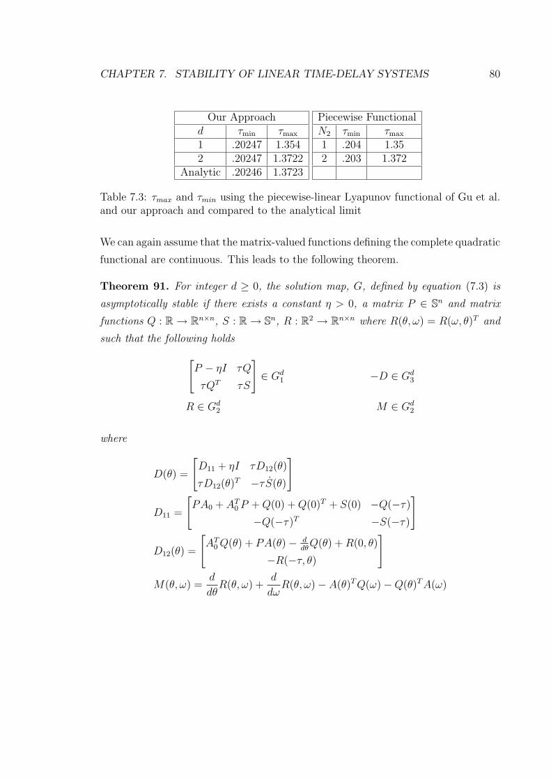
CHAPTER 7. STABILITY OF LINEAR TIME-DELAY SYSTEMS 80
Our Approachd τmin τmax
1 .20247 1.3542 .20247 1.3722
Analytic .20246 1.3723
Piecewise FunctionalN2 τmin τmax
1 .204 1.352 .203 1.372
Table 7.3: τmax and τmin using the piecewise-linear Lyapunov functional of Gu et al.and our approach and compared to the analytical limit
We can again assume that the matrix-valued functions defining the complete quadratic
functional are continuous. This leads to the following theorem.
Theorem 91. For integer d ≥ 0, the solution map, G, defined by equation (7.3) is
asymptotically stable if there exists a constant η > 0, a matrix P ∈ Sn and matrix
functions Q : R→ Rn×n, S : R→ Sn, R : R2 → Rn×n where R(θ, ω) = R(ω, θ)T and
such that the following holds
[P − ηI τQ
τQT τS
]∈ Gd
1 −D ∈ Gd3
R ∈ Gd2 M ∈ Gd
2
where
D(θ) =
[D11 + ηI τD12(θ)
τD12(θ)T −τ S(θ)
]
D11 =
[PA0 + AT
0 P + Q(0) + Q(0)T + S(0) −Q(−τ)
−Q(−τ)T −S(−τ)
]
D12(θ) =
[AT
0 Q(θ) + PA(θ)− ddθ
Q(θ) + R(0, θ)
−R(−τ, θ)
]
M(θ, ω) =d
dθR(θ, ω) +
d
dωR(θ, ω)− A(θ)T Q(ω)−Q(θ)T A(ω)
CHAPTER 7. STABILITY OF LINEAR TIME-DELAY SYSTEMS 81
Proof. We consider the complete quadratic functional
V (φ) =1
τ
∫ 0
−τ
[φ(0)
φ(θ)
]T [P − ηI τQ(θ)
τQ(θ)T τS(θ)
][φ(0)
φ(θ)
]T
dθ
+
∫ 0
−τ
∫ 0
−τ
φ(θ)T R(θ, ω)φ(ω)dθdω + η‖φ(0)‖2 ≥ η‖φ(0)‖2
The system is asymptotically stable if the Lie derivative is strictly negative. The Lie
derivative of the functional along trajectories of the system is given by
V (Γ(φ, 0)) =
∫ 0
−τ
φ(0)
φ(−τ)
φ(θ)
T
D(θ)
φ(0)
φ(−τ)
φ(θ)
dθ
−∫ 0
−τ
∫ 0
−τ
φ(θ)T M(θ, ω)φ(ω)dωdθ − η‖φ(0)‖2 ≤ −η‖φ(0)‖2
Thus, if the conditions of the theorem hold, then the system is asymptotically stable.
7.4 Conclusion
In this chapter, we have shown how to compute solutions to an operator-theoretic
version of the Lyapunov inequality. Our approach is to combine results from real alge-
braic geometry with functional analysis in order to parameterize certain convex cones
of positive operators using the convex cone of positive semidefinite matrices. We then
show that the operator inequalities can be expressed using affine constraints on these
matrices. This allows us to compute solutions using semidefinite programming, for
which there exist efficient numerical algorithms. We have further extended our results
to the case when the dynamics contain parametric uncertainty using a construction
based on certain results of Putinar and others. The numerical examples given in this
Chapter demonstrate a quick convergence to the analytic limit of stability.
CHAPTER 7. STABILITY OF LINEAR TIME-DELAY SYSTEMS 82
We conclude by mentioning that the methods of this chapter can be used to con-
struct full-rank solutions of the Lyapunov inequality. Furthermore, we have developed
methods for constructing the inverses of these full-rank operators. By computing so-
lutions to the Lyapunov inequality for the adjoint system constructed by Delfour and
Mitter [8], this invertibility result seems to imply that one can construct stabiliz-
ing controllers for linear time-delay systems. This work is ongoing, however, and is
therefore not detailed in this thesis.
Chapter 8
Stability of Nonlinear Time-Delay
Systems
8.1 Introduction
The question of stability of nonlinear functional differential equations is complicated
by the lack of a complete Lyapunov functional structure whose existence is necessary
for stability of a general nonlinear time-delay system. For this reason all results given
in this section will only be sufficient. Furthermore, we cannot claim, as was done
in the previous chapter, that these conditions will generally approach necessity in
any sense. Given these limitations, we felt that the best approach was to construct
a sequence of conditions that would approach necessity in at least one special case,
that of linear systems. For this reason, the conditions presented in this chapter are
a generalization of those in the previous one and the Lyapunov functionals reduce to
the complete quadratic functional in the case where the degree of x is restricted to
2. This chapter differs from the presentation of the linear case in that it includes a
section on delay-independent stability, a topic not previously discussed.
83

CHAPTER 8. STABILITY OF NONLINEAR TIME-DELAY SYSTEMS 84
8.2 Delay-Dependent Stability
Consider a nonlinear discrete time-delay system defined by a functional of the follow-
ing form for τi < τi−1 for i = 1, . . . , K and τ0 = 0.
f(xt) = f(x(t), x(t− τ1), · · · , x(t− τK))
In this section, we present conditions for stability based on the use of a gener-
alization of the compete quadratic functional. The generalized Lyapunov functional
has the following form.
V (φ) :=
∫ 0
−τK
Zd[φ(0), φ(θ)]T M(θ)Zd[φ(0), φ(θ)]dθ
+
∫ 0
−τK
∫ 0
−τK
Zd[φ(θ)]T R(θ, ω)Zd[φ(ω)]dθdω
8.2.1 Single Delay Case
In this subsection, we consider the special case of a single delay.
x(t) = f(x(t), x(t− τ))
Here we assume x(t) ∈ Rn and f is continuous. We first introduce some notation.
Definition 92. We say a continuous function f : R2n × R → R satisfies f ∈ K1 if
there exists some α > 0 such that the following holds for all φ ∈ Cτ .
∫ 0
−τ
f(φ(0), φ(θ), θ)dθ ≥ α‖φ(0)‖2
Definition 93. We say a continuous function f : R3n × R2 → R satisfies f ∈ K2 if
the following holds for all φ ∈ Cτ .
∫ 0
−τ
∫ 0
−τ
f(φ(θ), φ(ω), θ, ω)dθdω ≥ 0
CHAPTER 8. STABILITY OF NONLINEAR TIME-DELAY SYSTEMS 85
Definition 94. We say a continuous function f : R3n × R → R satisfies f ∈ K3 if
there exists some α > 0 such that the following holds for all φ ∈ Cτ .
∫ 0
−τ
f(φ(0), φ(−τ), φ(θ), θ)dθ ≥ α‖φ(0)‖2
The sets K1, K2, and K3 are used to define a positive Lyapunov functional and
some of its derivative forms. For a given degree bound, these sets can be parameterized
by the space of positive semidefinite matrices using the following subsets.
Definition 95. Denote f ∈ Ξd1 ⊂ K1 if f is a polynomial of degree d or less such
that there exists a polynomial function t : Rn×R→ R, of degree d or less, and α > 0
such that the following holds.
f(x1, x2, θ)− t(x1, θ)− α‖x1‖2 ∈ Σs∫ 0
−τ
t(x1, θ)dθ = 0
Definition 96. Denote f ∈ Ξ2d2 ⊂ K2 if f is a polynomial of degree 2d or less
and there exists a polynomial matrix function R : R2 → R(n+dd )×(n+d
d ) such that R ∈G2d
2 (defined in Chapter 7) and the following holds.
f(x1, x1, θ, ω) = Zd(x1)T R(θ, ω)Zd(x2) (8.1)
Definition 97. Denote f ∈ Ξd3 ⊂ K3 if f is a polynomial of degree d or less such
that there exist polynomial function t : R2n × R → R, of degree d or less, and α > 0
such that the following holds.
f(x1, x2, x3, θ)− t(x1, x2, θ)− α‖x1‖2 ∈ Σs∫ 0
−τ
t(x1, x2, θ)dθ = 0
We now state the stability theorem.
Theorem 98. For a given integer d ≥ 0, suppose there exist functions g ∈ Ξd1,
CHAPTER 8. STABILITY OF NONLINEAR TIME-DELAY SYSTEMS 86
h, h ∈ Ξd2, and −g ∈ Ξd
3 such that the following conditions hold.
g(xt(0), xt(−τ), xt(θ), θ)
= g(xt(0), xt(0), 0)− g(xt(0), xt(−τ),−τ)
+ τ∇xt(0)g(xt(0), xt(θ), θ)T f(xt(0), xt(−τ))− τ
δ
δθg(xt(0), xt(θ), θ)
+ τh(xt(0), xt(θ), 0, θ)− τh(xt(−τ), xt(θ),−τ, θ)
+ τh(xt(θ), xt(0), θ, 0)− τh(xt(θ), xt(−τ), θ,−τ)
h(xt(θ), xt(ω), θ, ω) =δ
δθh(xt(θ), xt(ω), θ, ω) +
δ
δωh(xt(θ), xt(ω), θ, ω)
Then the time-delay system defined by f is globally asymptotically stable.
Proof. Consider the Lyapunov functional defined as follows
V (xt) :=
∫ 0
−τ
g(xt(0), xt(θ), θ)dθ +
∫ 0
−τ
∫ 0
−τ
h(xt(θ), xt(ω), θ, ω)dθdω ≥ α‖xt(0)‖2
The derivative of this functional along trajectories of the systems can be expressed
as follows.
V (xt) :=g(xt(0), xt(0), 0)− g(xt(0), xt(−τ),−τ)
+
∫ 0
−τ
(∇xt(0)g(xt(0), xt(θ), θ)
T p(xt(0), xt(−τ))− δ
δθg(xt(0), xt(θ), θ)
)dθ
+
∫ 0
−τ
(h(xt(0), xt(θ), 0, θ)− h(xt(−τ), xt(θ),−τ, θ)
)dθ
+
∫ 0
−τ
(h(xt(θ), xt(0), θ, 0)− h(xt(θ), xt(−τ), θ,−τ)
)dθ
−∫ 0
−τ
∫ 0
−τ
( δ
δθh(xt(θ), xt(ω), θ, ω) +
δ
δωh(xt(θ), xt(ω), θ, ω)
)dθdω
=1
τ
∫ 0
−τ
g(xt(0), xt(−τ), xt(θ), θ)dθ +
∫ 0
−τ
∫ 0
−τ
h(xt(θ), xt(ω), θ, ω)dθdω
≤− α‖xt(0)‖2
Thus, we have that if the conditions of the theorem are satisfied, then the derivative

CHAPTER 8. STABILITY OF NONLINEAR TIME-DELAY SYSTEMS 87
of the Lyapunov functional is negative definite, proving global asymptotic stability of
the functional differential equation defined by f .
As with the linear case, the conditions contained in Theorem 98 can be expressed
as a semidefinite program.
8.2.2 Multiple Delays
In this section, we consider stability of nonlinear time-delay systems defined by func-
tionals of the following form for τi < τi−1 for i = 1, . . . , K and τ0 = 0.
x(t) = f(x(t), x(t− τ1), · · · , x(t− τK))
As before, x(t) ∈ Rn, f is continuous, and we introduce some notation.
Definition 99. We say a function f : R2n×R→ R satisfies f ∈ K1 if f(x1, x2, θ) is
continuous except possibly at points θ ∈ −τiK−1i=1 and there exists some α > 0 such
that the following holds for all φ ∈ Cτ .
∫ 0
−τK
f(φ(0), φ(θ), θ)dθ ≥ α‖φ(0)‖2
Definition 100. We say a function f : Rn×R2 → R satisfies f ∈ K2 if f(x1, x2, θ, ω)
is continuous except possibly at points θ, ω ∈ −τiK−1i=1 and the following holds for all
φ ∈ Cτ . ∫ 0
−τK
∫ 0
−τK
f(φ(θ), φ(ω), θ, ω)dθdω ≥ 0
Definition 101. We say a function f : Rn(K+2) × R → R satisfies f ∈ K3 if f is
continuous except possibly at points θ ∈ −τiKi=1 and there exists some α > 0 such
that the following holds for all φ ∈ Cτ .
∫ 0
−τK
f(φ(0), φ(−τ1), · · · , φ(−τK), φ(θ), θ)dθ ≥ α‖φ(0)‖2
The sets K1, K2, and K3 are used to define positive Lyapunov functionals and
some of its derivative forms in the case of multiple delays. For a given degree bound,

CHAPTER 8. STABILITY OF NONLINEAR TIME-DELAY SYSTEMS 88
these sets can be parameterized by the space of positive semidefinite matrices using
the following subsets.
Definition 102. Denote f ∈ Ξd1 ⊂ K1 if there exist polynomial functions fi : R2n ×
R → R, ti : Rn × R → R, i = 1 · · ·K of degree d or less and α > 0 such that the
following holds for all xi ∈ Rn.
fi(x1, x2, θ)− ti(x1, θ)− α‖x1‖2 ∈ Σs
f(x1, x2, θ) = fi(x1, x2, θ) ∀θ ∈ [−τi,−τi−1]
K∑i=1
∫ −τi−1
−τi
ti(x1, θ)dθ = 0
Definition 103. Denote f ∈ Ξ2d2 ⊂ K2 if f is a polynomial of degree 2d or less such
there exists a matrix function R : R2 → R(n+dd )×(n+d
d ) such that R ∈ G2d2 and the
following holds.
f(x1, x1, θ, ω) = Zd(x1)T R(θ, ω)Zd(x2) (8.2)
Definition 104. Denote f ∈ Ξd3 ⊂ K3 if there exist functions fi : Rn(K+2) × R→ R,
ti : Rn(K+2) × R → R, i = 1 · · ·K, of degree d or less, and α > 0 such that the
following holds.
fi(x1, · · · , xK+1, xK+2, θ)− ti(x1, · · · , xK+1, θ)− α‖x1‖2 ∈ Σs
f(x1, · · · , xK+1, xK+2, θ) = fi(x1, · · · , xK+1, xK+2, θ) ∀θ ∈ [−τi,−τi−1]
K∑i=1
∫ −τi−1
−τi
ti(x1, · · · , xK+1, θ)dθ = 0
We now state the stability theorem in the case of multiple delays.
Theorem 105. For a given integer d ≥ 0, suppose there exist functions h ∈ Ξd1,
g, g ∈ Ξd2, and h ∈ Ξd
3 such that the following conditions hold where Ii := [−τi,−τi−1]
CHAPTER 8. STABILITY OF NONLINEAR TIME-DELAY SYSTEMS 89
and ∆τi := τi − τi−1.
gi(xt(0), · · · , xt(−τK), xt(θ), θ)
= gi(xt(0), xt(−τi−1),−τi−1)− gi(xt(0), xt(−τi),−τi)
+ ∆τi∇xt(0)gi(xt(0), xt(θ), θ)T f(xt(0), · · · , xt(−τK))−∆τi
δ
δθgi(xt(0), xt(θ), θ)
+K∑
j=1
(hij(xt(−τi−1, xt(θ),−τi−1, θ)− hij(xt(−τi), xt(θ),−τi, θ)
)
+K∑
j=1
(hji(xt(θ), xt(−τj−1), θ,−τj−1)− hji(xt(θ), xt(−τj), θ,−τj)
)
hij(xt(θ), xt(ω), θ, ω) =δ
δθhij(xt(θ), xt(ω), θ, ω) +
δ
δωhij(xt(θ), xt(ω), θ, ω)
Where
∆τigi(xt(0), xt(θ), θ) := g(xt(0), xt(θ), θ) ∀θ ∈ Ii
gi(xt(0), · · · , xt(−τK), xt(θ), θ) := g(xt(0), · · · , xt(−τK), xt(θ), θ) ∀θ ∈ Ii
hij(xt(θ), xt(ω), θ, ω) := h(xt(θ), xt(ω), θ, ω) ∀θ, ω ∈ Ii
hij(xt(θ), xt(ω), θ, ω) := h(xt(θ), xt(ω), θ, ω) ∀θ, ω ∈ Ii
Then the time-delay system defined by f is globally asymptotically stable.
Proof. Consider the Lyapunov functional defined as follows.
V (xt) :=
∫ 0
−τK
g(xt(0), xt(θ), θ)dθ +
∫ 0
−τK
∫ 0
−τK
h(xt(θ), xt(ω), θ, ω)dθdω
=K∑
i=1
∫ −τi−1
−τi
∆τigi(xt(0), xt(θ), θ)dθ +K∑
i,j=1
∫ −τi−1
−τi
∫ −τj−1
−τj
hij(xt(θ), xt(ω), θ, ω)dθdω
≥ α‖xt(0)‖2
The inequality holds for some α > 0 by definition of the set K1. The derivative of

CHAPTER 8. STABILITY OF NONLINEAR TIME-DELAY SYSTEMS 90
this functional along trajectories of the system can be expressed as follows.
V (xt) :=K∑
i=1
∆τi
(gi(xt(0), xt(−τi−1),−τi−1)− gi(xt(0), xt(−τi),−τi)
)
+K∑
i=1
∫ −τi−1
−τi
∆τi
(∇xt(0)gi(xt(0), xt(θ), θ)
T f(xt(0), · · · , xt(−τK))− δ
δθgi(xt(0), xt(θ), θ)
)dθ
+K∑
i,j=1
∫ −τi−1
−τi
(hij(xt(−τj−1, xt(ω),−τj−1, ω)− hij(xt(−τj), xt(ω),−τj, ω)
)dω
+K∑
i,j=1
∫ −τj−1
−τj
(hij(xt(θ), xt(−τi−1), θ,−τi−1)− hij(xt(θ), xt(−τi), θ,−τi)
)dθ
−K∑
i,j=1
∫ −τi−1
−τi
∫ −τj−1
−τj
( δ
δθhij(xt(θ), xt(ω), θ, ω) +
δ
δωhij(xt(θ), xt(ω), θ, ω)
)dθdω
=1
τK
K∑i=1
∫ −τi−1
−τi
gi(xt(0), · · · , xt(−τK), xt(θ), θ)dθ
+K∑
i,j=1
∫ −τi−1
−τi
∫ −τj−1
−τj
hij(xt(θ), xt(ω), θ, ω)dθdω
=
∫ 0
−τ
g(xt(0), · · · , xt(−τK), θ)dθ +
∫ 0
−τ
∫ 0
−τ
h(xt(θ), xt(ω), θ, ω)dθdω ≤ −α‖xt(0)‖2
The final inequality follows from the definition of K2 and K3. Thus the conditions of
the theorem imply global asymptotic stability of the time-delay system defined by f .
Similar to the case of a single delay, the conditions of Theorem 105 can be ex-
pressed as a semidefinite program.
8.3 Delay-Independent Stability
We now briefly discuss conditions for delay-independent stability of time-delay sys-
tems. Recall that a system defined by a functional of the following form is stable

CHAPTER 8. STABILITY OF NONLINEAR TIME-DELAY SYSTEMS 91
independent of delay if it is stable for any finite values of τiKi=1.
f(xt) := f(xt(0), xt(−τ1), · · · , xt(−τK))
Here we assume f is continuous and x(t) ∈ Rn. The theorems of the previous
section can be applied directly to the problem of delay-independent stability by con-
sidering τi to be an uncertain parameter and searching for a parameter-dependent
Lyapunov functional. However, a less computationally intensive approach is to con-
sider specific Lyapunov functional forms where τi does not explicitly appear in the
stability conditions. One such Lyapunov functional form is given as follows.
V (φ) = p0(φ(0)) +K∑
i=1
∫ 0
−τi
pi(φ(θ)) dθ
This functional has an upper Lie derivative defined as follows.
V (φ) = ∇p0(φ(0))T f(xt(0), xt(−τ1), · · · , xt(−τK)) +K∑
i=1
pi(φ(0))− p2(φ(−τi))
Since τi does not appear explicitly in the derivative of the functional, we can prove
stability for arbitrary τi using the following theorem.
Theorem 106. For a given integer d, suppose there exist functions piKi=0 and con-
stant α > 0 such that pi(0) = 0 for i = 0, . . . , K and the following conditions hold for
all xi ∈ Rn.
p0(x0)− α‖x0‖2 ∈ Σds
pi(xi) ∈ Σds i = 1, . . . , K
−∇p0(x0)T f(x0, x1, · · · , xK)−
K∑i=1
(pi(x0)− p2(xi)
)− α‖x0‖2 ∈ Σs
Then the system defined by f is globally asymptotically stable for any finite values of
τi.

CHAPTER 8. STABILITY OF NONLINEAR TIME-DELAY SYSTEMS 92
Proof. Consider the following Lyapunov functional.
V (xt) = p0(xt(0)) +K∑
i=1
∫ 0
−τi
pi(xt(θ)) dθ ≥ α‖xt(0)‖2
The Lyapunov functional is positive definite by the conditions of the theorem. The
derivative of the functional along trajectories of the system is given as follows.
V (φ) = ∇p0(φ(0))T f(xt(0), xt(−τ1), · · · , xt(−τK))+K∑
i=1
pi(φ(0))−p2(φ(−τi)) ≤ −α‖xt(0)‖2
Therefore the derivative is negative definite by the conditions of the theorem. There-
fore we have that the system defined by f is globally asymptotically stable for any
finite values of τi.
The computational burden associated with the conditions expressed in Theo-
rem 106 is significantly less than that associated with proving delay-independent
stability using Theorem 105. This reduction occurs because in this case, we have ex-
plicitly chosen a Lyapunov functional structure where the delays τi do not explicitly
appear in the derivative. Naturally, the use of a more specialized Lyapunov func-
tional structure may result in an increased level of conservativity. For this reason,
when testing delay-independent stability, it is recommended that Theorem 106 be
used as a first approximation and that Theorem 105 be used if additional accuracy is
required.
8.3.1 Numerical Examples
The contribution of this chapter is to show that Lyapunov functions to prove stability
of arbitrary non-linear polynomial systems may be computed algorithmically. To
illustrate this, we compare our results with those derived through less algorithmic
analysis.
Example 1: Reflection Dynamics
To begin, we compare our results with a solution given by Hale [14] and attributed

CHAPTER 8. STABILITY OF NONLINEAR TIME-DELAY SYSTEMS 93
0 1 2 3 4 5 6 7 8 9 100
0.2
0.4
0.6
0.8
1
1.2
1.4
1.6
1.8
2
time
x(t)
x(t) vs. time for a delay of 1 second
Figure 8.1: Example of a trajectory of x(t) for a = −1, b = .9
0 1 2 3 4 5 6 7 8 9 100
50
100
150
200
250
300
350Lyapunov−Krasovskii functional over time for 1s delay
time
p1(x(t))
p2(x(t))
V(xt)
Figure 8.2: Example of a trajectory of V (xt) for a = −1, b = .9
to LaSalle for the following dynamics.
x(t) = ax3(t) + bx3(t− τ) (8.3)
The following Lyapunov function is used by Hale to show that the system is stable
for any a < 0, |b| < |a|.
V (xt) = −x4t (0)
2a+
∫ 0
−τ
x6t (θ) dθ (8.4)
Our own computation of various points give similar results. For example, for
a = −1, b = .9, we can prove asymptotic stability using the following function
V (xt) = −3.92x2t (0) + 1.91x4
t (0) +
∫ 0
−τ
5.35x4t (θ) + 3.72x6
t (θ) dθ
The purpose here is not to construct this particular Lyapunov function, but rather

CHAPTER 8. STABILITY OF NONLINEAR TIME-DELAY SYSTEMS 94
to demonstrate that such functions can be numerically computed without the insight
needed to manually derive the results. To illustrate this expanded flexibility, suppose
we introduce a cross-term, such as might arise due to interference, then we have
x(t) = ax3(t) + c(x(t)x(t− τ))2 + bx3(t− τ) (8.5)
We find the following Lyapunov function in the case when a = −1, b = 0.5, c = 0.2.
V (xt) = 4.233x2t (0)−0.2147x3
t (0)+1.856x4t (0)
∫ 0
−τ
4.107x4t (θ)+0.1525x5
t (θ)+3.454x6t (θ) dθ
Example 2: Epidemiology
We now consider the following epidemiological model. Consider a human popu-
lation subject to non-lethal infection by a virus. Assume the disease has incubation
period τ . Cooke [6] models the percentage of infected population, y(t) using the
following dynamics.
y(t) = −ay(t) + by(t− τ)(1− y(t)
)
Where
• a is the recovery rate for the infected population.
• b is the rate of infection for those exposed to the virus.
The model is nonlinear and equilibria exist at y∗ = 0 and y∗ = (b − a)/b. Cooke
used the following Lyapunov functional to prove delay-independent stability of the 0
equilibrium for a > b > 0.
V (φ) =1
2φ(0)2 +
1
2
∫ 0
−τ
aφ(θ)2dθ
Using semidefinite programming, we were also able to prove delay-independent
stability for a > b > 0 using the following functional.
V (φ) = 1.75φ(0)2 +
∫ 0
−τ
(1.47a + .28b)φ(θ)2dθ
CHAPTER 8. STABILITY OF NONLINEAR TIME-DELAY SYSTEMS 95
The point of these examples is obviously not to trivialize the work of Cooke and
Hale, but rather to show the broad applicability and utility of the algorithms presented
in this thesis.
8.4 Conclusion
This chapter provides a generalization of the stability analysis results for linear time-
delay systems presented in Chapter 7 to the case of nonlinear dynamics. To this end,
we have proposed a sequence of sufficient conditions for both delay-dependent and
delay independent stability of nonlinear systems with multiple delays. The numerical
examples presented illustrate that many previous results on stability analysis can be
derived using our algorithmic framework. Unfortunately, unlike in the linear stability
case, we are not optimistic that the results of this chapter will lead to algorithms
for the construction of stabilizing controllers for any broad class of nonlinear time-
delay systems. This is because the results of this chapter to not fit as neatly into the
operator-theoretic framework of the linear case.
Appendix A
Appendix to Chapter 2
Additional Notation: Denote the complete metric space
Vα := x ∈ C[−τ,∞) : x(θ) = φ(θ) for θ ∈ [−τ, 0], supt≥−τ
‖x(t)‖e−αt < ∞,
which has the following metric.
d(x, y)Vα = supt≥−τ
‖x(t)− y(t)‖e−αt
Define Cτ to be the space of continuous functions defined on [−τ, 0] with norm
‖x‖Cτ = supt∈[−τ,0]
‖x(t)‖2.
For a given functional f : Cτ × R+ → Rn, let Λ be defined by
(Λx)(t) = φ(0) +
∫ t
0
f(xs, s)ds for all t ≥ 0
and (Λx)(t) = φ(t) for t ∈ [−τ, 0).
Definition 107. We say that a functional f : Cτ ×R+ → Rn satisfies Assumptions
1 if
96

APPENDIX A. APPENDIX TO CHAPTER 2 97
• There exists a K1 > 0 such that
‖f(x, t)− f(y, t)‖2 ≤ K1‖x− y‖Cτ for all x, y ∈ Cτ , t ≥ 0
• There exists a K2 > 0 such that
‖f(0, t)‖ ≤ K2 for all t ≥ 0
• f(x, t) is jointly continuous in x and t. i.e. for every (x, t) and ε > 0, there
exists a η > 0 such that
‖x− y‖Cτ + ‖t− s‖ ≤ η ⇒ ‖f(x, t)− f(y, s)‖ ≤ ε.
Definition 108. Given a functional f : Cτ × R+ → Rn, we say that a function
x ∈ C[−τ,∞) is a solution to Problem 1 with initial condition φ ∈ Cτ if x is
differentiable for t ≥ 0, x(t) = φ(t) for t ∈ [−τ, 0] and
x(t) = f(xt, t) for all t ≥ 0
Results:
Lemma 109. If f : Cτ × R+ → Rn satisfies Assumptions 1, and x is a continuous
function, then f(xt, t) is a continuous function in t.
Proof. If f : Cτ × R+ → Rn satisfies Assumptions 1, then for any t1, ε > 0, there
exists a η1 > 0 such that
‖xt1 − xt2‖Cτ + ‖t1 − t2‖ ≤ η1 ⇒ ‖f(xt1 , t1)− f(xt2 , t2)‖ ≤ ε.
Now if x(t) is a continuous function of t, then for any t1 ≥ 0, x(t) is uniformly
continuous on the interval It1 := [max−τ, t1− τ − .1, t1 + .1]. Hence, for any ε2 > 0,
there exists a η2 > 0 such that for s1, s2 ∈ It1 , we have that
|s1 − s2| ≤ η2 ⇒ ‖x(s1)− x(s2)‖2 ≤ ε2.

APPENDIX A. APPENDIX TO CHAPTER 2 98
Now for a given t1 ≥ 0 and ε > 0, let η1 be defined as above. Let ε2 = η1/2 define η2.
Then if η = min.1, η2, η1/2, we have that |t1 − t2| ≤ η implies that
‖xt1 − xt2‖Cτ = supθ∈[−τ,0]
‖xt1(θ)− xt2(θ)‖2
= supθ∈[−τ,0]
‖x(t1 + θ)− x(t2 + θ)‖2 ≤ ε2 = η1/2.
This holds since ‖(t1 + θ)− (t2 + θ)‖ = ‖t1 − t2‖ ≤ η2 means ‖x(t1 + θ)− x(t2 + θ)‖2 ≤ε2 since t1 + θ ∈ It1 for θ ∈ [−τ, 0] and t2 + θ ∈ It1 for ‖t1 − t2‖ < .1, θ ∈ [−τ, 0] and
t2 ≥ 0. Therefore we have that
‖xt1 − xt2‖Cτ + ‖t1 − t2‖ ≤ η1/2 + η1/2 = η1.
This implies that
‖f(xt1 , t1)− f(xt2 , t2)‖ ≤ ε.
Thus we have continuity of f(xt, t).
Lemma 110. Suppose f : Cτ ×R+ → Rn satisfies Assumptions 1, then Λ : Vα → Vα.

APPENDIX A. APPENDIX TO CHAPTER 2 99
Proof. Suppose x ∈ Vα. Let y = Λx. Then y(t) = φ(t) for t ∈ [−τ, 0], y is
continuous, and the following holds for t ≥ 0.
‖y(t)‖2 = ‖φ(0) +
∫ t
0
f(xs, s)ds‖2
≤ ‖φ(0)‖2 + ‖∫ t
0
f(xs, s)ds‖2
≤ ‖φ(0)‖2 +
∫ t
0
‖f(xs, s)‖2ds
= ‖φ(0)‖2 +
∫ t
0
‖f(xs, s)− f(0, s) + f(0, s)‖2ds
≤ ‖φ(0)‖2 +
∫ t
0
‖f(xs, s)− f(0, s)‖2 + ‖f(0, s)‖2ds
≤ ‖φ(0)‖2 +
∫ t
0
K1‖xs‖Cτ + K2ds
= ‖φ(0)‖2 + K1
∫ t
0
supθ∈[−τ,0]
‖xs(θ)‖2ds + K2t
= ‖φ(0)‖2 + K1
∫ t
0
supθ∈[−τ,0]
‖x(s + θ)‖2ds + K2t
Now, since x ∈ Vα, there exists some c > 0 such that ‖x(t)‖2 ≤ ceαt for all t ≥ −τ .
Therefore, supθ∈[−τ,0]‖x(t + θ)‖ ≤ ceαt for all t ≥ 0. Therefore, we have the following
for t ≥ 0.
‖y(t)‖2 ≤ ‖φ(0)‖2 + K1
∫ t
0
supθ∈[−τ,0]
‖x(s + θ)‖2ds + K2t
≤ ‖φ(0)‖2 + K1
∫ t
0
ceαsds + K2t
= ‖φ(0)‖2 +cK1
α(eαt − 1) + K2t

APPENDIX A. APPENDIX TO CHAPTER 2 100
Thus
supt≥0‖y(t)‖2e
−αt ≤ supt≥0
(‖φ(0)‖2e
−αt +cK1
α(1− e−αt) + K2te
−αt
)
≤ ‖φ(0)‖2 +cK1
α+
eK2
α= c1.
Now let c2 = supθ∈[−τ,0]‖φ(θ)‖ and c = maxc1, c2. Then supt≥−τ‖y(t)‖2e−αt ≤ c.
Thus y ∈ Vα.
Lemma 111. Suppose f : Cτ×R+ → Rn satisfies Assumptions 1, and K1 < α. Then
Λ is a contraction on Vα.
Proof. Suppose x, y ∈ Vα. Then we have the following for t ≥ 0.
‖Λx(t)− Λy(t)‖2 = ‖∫ t
0
f(xs, s)− f(ys, s)ds‖2
≤∫ t
0
‖f(xs, s)− f(ys, s)‖2ds
≤∫ t
0
K1‖xs − ys‖Cτ ds
= K1
∫ t
0
supθ∈[−τ,0]
‖xs(θ)− ys(θ)‖2ds
= K1
∫ t
0
supθ∈[−τ,0]
‖x(s + θ)− y(s + θ)‖2ds
= K1
∫ t
0
supθ∈[s−τ,s]
‖x(θ)− y(θ)‖2ds
Now recall that d(x, y)Vα = supt≥−τ‖x(t)− y(t)‖e−αt. Therefore, ‖x(t)− y(t)‖2 ≤d(x, y)Vαeαt for all t ≥ −τ . Thus supθ∈[t−τ,t]‖x(θ)− y(θ)‖2 ≤ d(x, y)eαt for all t ≥ 0.

APPENDIX A. APPENDIX TO CHAPTER 2 101
Thus we have the following for all t ≥ 0.
‖Λx(t)− Λy(t)‖2 ≤ K1
∫ t
0
supθ∈[s−τ,s]
‖x(θ)− y(θ)‖2ds
≤ K1
∫ t
0
d(x, y)Vαeαsds
=K1
αd(x, y)Vα(eαt − 1)
Therefore
d(Λx, Λy)Vα = supt≥−τ
‖Λx(t)− Λy(t)‖2e−αt
= supt≥0‖Λx(t)− Λy(t)‖2e
−αt
≤ supt≥0
K1
αd(x, y)Vα(1− e−αt)
≤ K1
αd(x, y)Vα < d(x, y)Vα
Therefore Λ is a contraction on Vα.
Lemma 112 (Existence). Suppose f satisfies Assumptions 1, x ∈ Vα, and x = Λx.
Then x is a solution of Problem 1. i.e. x is differentiable , x(t) = φ(t) for t ∈ [−τ, 0]
and
x(t) = f(xt, t) for all t ≥ 0.
Proof. Since x ∈ Vα, x is continuous and x(t) = φ(t) for t ∈ [−τ, 0]. Furthermore,
since x = Λx, we have that
x(t) = φ(0) +
∫ t
0
f(xs, s)ds.
Since x is continuous and f satisfies Assumptions 1, by Lemma 109 we have that
f(xs, s) is a continuous and integrable function on [0, t]. Now, since x(t) − x(0) =∫ t
0f(xs, s)ds, we have by the fundamental theorem of Calculus(v1) that x(t) − x(0)
APPENDIX A. APPENDIX TO CHAPTER 2 102
is differentiable and
x(t) = f(xt, t).
Lemma 113 (Uniqueness). Suppose f satisfies Assumptions 1, then any solution
to Problem 1 is unique.
Proof. Suppose x and y are solutions to Problem 1. Define p as follows for t ≥ 0.
p(t) = supθ∈[t−τ,t]
‖x(θ)− y(θ)‖2
= supθ∈[t−τ,t],θ≥0
‖x(θ)− y(θ)‖2
= supθ∈[t−τ,t],θ≥0
‖∫ θ
0
f(xs, s)− f(ys, s)ds‖2
≤ supθ∈[t−τ,t],θ≥0
∫ θ
0
‖f(xs, s)− f(ys, s)‖2ds
≤ supθ∈[t−τ,t],θ≥0
K1
∫ θ
0
‖xs − ys‖Cτ ds
= supθ∈[t−τ,t],θ≥0
K1
∫ θ
0
supω∈[s−τ,s]
‖x(ω)− y(ω)‖2ds
= supθ∈[t−τ,t],θ≥0
K1
∫ θ
0
p(s)ds
Now let q(t) =∫ t
0p(s)ds. Then q(0) = 0 and q(t) = p(t) ≥ 0 for all t ≥. Therefore, q
is non-negative and monotonically increasing. Thus we have the following.
q(t) ≤ supθ∈[t−τ,t],θ≥0
K1
∫ θ
0
p(s)ds
≤ supθ∈[t−τ,t],θ≥0
K1q(θ) = K1q(t)
APPENDIX A. APPENDIX TO CHAPTER 2 103
Therefore, we have that q(t)−K1q(t) ≤ 0 for all t ≥ 0. Which implies the following
for g(t) = q(t)e−K1t, t ≥ 0.
g(t) =d
dt
(q(t)e−K1t
)= e−K1t (q(t)−K1q(t)) ≤ 0
Since g(0) = q(0) = 0 and g(t) ≤ 0 for all t ≥ 0, we have that g(t) ≤ 0 for all
t ≥ 0. However, g(t) ≤ 0 implies q(t) ≤ 0, and so we have that q(t) = 0 for all t ≥ 0.
Therefore, since q(t) = p(t) = 0 for all t ≥ 0 and p(0) = 0, we have that p(t) = 0 for
all t ≥ 0. This implies that x(t) = y(t) for all t ≥ 0, which implies that x = y. Thus
any solution to problem 1 is unique.
Theorem 114. Suppose a functional f : Cτ × R+ → Rn satisfies the following.
• There exists a K1 > 0 such that
‖f(x, t)− f(y, t)‖2 ≤ K1‖x− y‖Cτ for all x, y ∈ Cτ , t ≥ 0.
• There exists a K2 > 0 such that
‖f(0, t)‖ ≤ K2 for all t ≥ 0.
• f(x, t) is jointly continuous in x and t. i.e. for every (x, t) and ε > 0, there
exists a η > 0 such that
‖x− y‖Cτ + ‖t− s‖ ≤ η ⇒ ‖f(x, t)− f(y, s)‖ ≤ ε.
Then for any φ ∈ Cτ , there exists a unique x ∈ C[−τ,∞) such that x is differentiable
for t ≥ 0, x(t) = φ(t) for t ∈ [−τ, 0] and
x(t) = f(xt, t) for all t ≥ 0.
Proof. We have already shown by Lemmas 110 and 111 that Λ, as defined by f , is
a contraction on Vα for any α > K. Therefore, there exists some α > K, x ∈ Vα such
APPENDIX A. APPENDIX TO CHAPTER 2 104
that x = Λx. Therefore, by Lemma 112, we have that x is a solution. By Lemma 113,
we have that this solution is unique.
Lemma 115. Let
f(x, t) :=N∑
j=1
Ajx(t− τj) +
∫ 0
−τ
A(θ)x(t− θ)dθ,
where A(θ) is bounded on [−τ, 0]. Then there exists some K > 0 such that
‖f(x, t)− f(y, t)‖2 ≤ K‖x− y‖Cτ .
Proof. For A ∈ Rn×m, let σ(A) denote the maximum singular value of A. Then we
have the following.
‖f(x, t)− f(y, t)‖2
= ‖N∑
j=1
Aj(x(t− τj)− y(t− τj)) +
∫ 0
−τ
A(θ)(x(t− θ)− y(t− θ))dθ‖2
≤N∑
j=1
‖Aj(x(t− τj)− y(t− τj))‖2 +
∫ 0
−τ
‖A(θ)(x(t− θ)− y(t− θ))‖2dθ
≤N∑
j=1
σ(Aj)‖x(t− τj)− y(t− τj)‖2 +
∫ 0
−τ
σ(A(θ))‖x(t− θ)− y(t− θ)‖2dθ
≤N∑
j=1
σ(Aj)‖x− y‖Cτ +
∫ 0
−τ
σ(A(θ))dθ‖x− y‖Cτ
=
(N∑
j=1
σ(Aj) +
∫ 0
−τ
σ(A(θ))dθ
)‖x− y‖Cτ
Appendix B
Appendix to Chapter 6
Lemma 116. M ∈ Σs
⋂Sn
2d[x] if and only if there exists some matrix Q ∈ Rnzn×nzn,
where nz =(
n+dd
)such that Q ≥ 0 and the following holds.
M(x) =(Zn
d [x])T
QZnd [x]
Proof. Since M ∈ Σs, we know that there exist Gi ∈ Rn×n[x] for i = 1 . . . m such
that
M(x) =m∑
i=1
Gi(x)T Gi(x)
Now suppose that there exists some i′ and i0, j0 such that element [Gi′ ]i0,j0 of Gi′ is
of degree d > d. Then, since Mi0,i0(x) =∑m
i=1
∑k[Gi]k,i0(x)2, we have that Mi0,i0 is
of at least degree 2d. This is because a finite sum of squares of R[x] is of degree 2d,
where d is the maximum degree of the squared elements. However, since M ∈ Snd by
assumption, we have a contradiction. Therefore Gi ∈ Rn×nd [x]. Now, for any element
Gi ∈ Rn×nd [x], there exists a B ∈ Rn×n(dz) where dz is the length of Zd[x] such that
Gi(x) = BZnd [x]. Therefore we have that
M(x) =m∑
i=1
(Zn
d [x])T
BT BZnd [x] =
(Zn
d [x])T
QZnd [x],
where Q =∑m
i=1 BT B ≥ 0.
105
APPENDIX B. APPENDIX TO CHAPTER 6 106
Lemma 117. M ∈ Σs if and only if yT M(x)y ∈ Σs.
Proof. (⇐) Suppose f(x) = yT M(x)y ∈ Σs. Then f(x) =∑m
i=1 gi(x, y)2 =∑mi=1(bi(x)T y)2 where the bi are some vectors of functions. This follows since the gi
must be homogeneous of degree 1 in y. Therefore, we have the following.
yT M(x)y =m∑
i=1
yT bi(x)bi(x)T y
Thus M(x) =∑m
i=1 bi(x)bi(x)T . Therefore M(x) ∈ Σs.
(⇒) Now Suppose M ∈ Σs. Then for some Gi(x) ∈ Rn×n[x] for i = 1 . . .m, we
have that f(x) = yT M(x)y =∑m
i=1 yT GTi (x)Gi(x)y =
∑mi=1 gi(x, y)T gi(x, y), where
gi(x, y) = Gi(x)y. Therefore, f ∈ Σs.
Appendix C
Appendix to Chapter 5
Lemma 118. 0 ≤ f1(x)x ≤ βx2 where β = eατ p0−1
p0.
Proof. Recall f1(y) = mine
ατ
y − 1, eατ
p0 − 1.Let
c1(y) =e
ατ
y − 1
y.
We show that c1(y) ≥ 0 for all y.
c1(y) =(α
τy − 1)e
ατ
y + 1
y2.
c1(y) ≥ 0 for all y is and only if c2 := c1(y)y2 ≥ 0 for all y.
c2(y) = (α
τye
ατ
y.
Thus c2(y) < 0 for all y < 0 and c2(y) > 0 for all y > 0, therefore c2 has a global
minimum at y = 0. Since c2(0) = 0, we conclude that c2(y) ≥ 0 for all y and thus
c1(y) ≥ 0 for all y. Since c1 is monotone increasing, we have the following for all
y ≤ p0.
eατ
y − 1
y≤ e
ατ
p0 − 1
p0
.
107
APPENDIX C. APPENDIX TO CHAPTER 5 108
Thus for y ≤ p0.
(eατ
y − 1)y ≤ βy2.
Furthermore, limy→−∞ c1(y) = 0 therefore, c1(y) ≥ 0 for all y, thus
(eατ
y − 1)y ≥ 0.
Therefore, by the definition of f1, we have that 0 ≤ f1(x)x ≤ βx2.
Lemma 119. Let z = ∆zy with y ∈ W2, then limt→∞ z(t) = 0.
Proof. Let v = z = ∆y. Suppose that T2 > T1 > 0 and let H = PT2 − PT1 . Then
‖Hv‖22 =
∫ T2
T1
z(t)2dt
≤ β
∫ T2
T1
z(t)y(t) dt− β
∫ T2
T1
z(t)z(t) dt
= β〈Hv, Hy〉 − β
2(z(T2)
2 − z(T1)2)
≤ β‖Hv‖2‖Hy‖2 − β
2
(z(T2)
2 − z(T1)2)
Hence
z(T2)2 − z(T1)
2 ≤ 2‖Hv‖2‖Hy‖2 − 2
β‖Hv‖2
2
≤ 2‖Hv‖2‖Hy‖2
By Lemma 29, v ∈ L2. Since ‖v‖ and ‖y‖ exist, we can use the Cauchy criterion
and the above inequality to establish that for any δ > 0, there exists a Tδ such that
T2 > T1 > Tδ implies (z(T2)2 − z(T1)
2) < δ. It is shown in Lemma 122 that this
implies that for any infinite increasing sequence Ti, z(Ti)2 is a Cauchy sequence
and therefore z(t)2 converges to a limit. Since z is continuous, this implies that z(t)
also converges to a limit, z∞. Since y ∈ W2, we have limt→∞ y(t) = y∞ = 0. Recall
fc(a, b) = f1(b) at points such that a > −p0 or b > 0. Suppose z∞ 6= 0. If z∞ < 0, then

APPENDIX C. APPENDIX TO CHAPTER 5 109
y∞ − z∞ > 0 and fc(a, b) = f1(b) in some neighborhood of (z∞, y∞ − z∞). If z∞ > 0,
then z∞ > 0 ≥ −p0 and fc(a, b) = f1(b) in some neighborhood of (z∞, y∞−z∞). Since
f1 is continuous, we have limt→∞ z(t) = limt→∞ fc(z(t), y(t)− z(t)) = f1(y∞ − z∞) =
f1(−z∞). By inspection of the function f1, we see that z∞ 6= 0 implies that z has
a nonzero limit. However, since z ∈ L2, it cannot have a nonzero limit. Thus we
conclude by condradiction that z∞ = 0.
Lemma 120. If v = ∆y with y ∈ W2, then 〈v, y − v〉 ≥ −β|y(0)|2.
Proof. Let z = ∆zv and define the variable r(t) = y(t)− z(t) and the set M = t :
z(t) > −p0 or r(t) ≥ 0, then
〈v, y − v〉 = 〈z, y − z〉 =
∫ ∞
0
z(t)r(t)dt
=
∫
M
f1(r(t))r(t)dt ≤ β‖y‖‖y‖+ β2‖v‖2
Since y ∈ W2, we have that y is absolutely continuous and thus r is absolutely
continuous. Since r, z are absolutely continuous functions and since by Lemma 30,
we have z(t) → 0, we can partition the set M into the countable union of sequential
disjoint intervals⋃
i Ii
⋃If where Ii = [Ta,i, Tb,i) with Ta,i, Tb,i ⊂ R+ and If =
[Ta,f ,∞). To see that the intervals are closed on the left, suppose Ii were open on
the left. Then, since Ta,i 6∈ M , z(Ta,i) = −p0 and r(Ta,i) < 0. However, since r is
continuous, r(Ta,i + η) < 0 for η sufficiently small. Since r(t) < 0 implies z(t) ≤ 0, we
have that z(Ta,i + η) ≤ −p0 and thus Ta,i + η 6∈ M for η sufficiently small, which is a
contradiction. Thus all the intervals are closed on the left. Similarly, one can show
that all the intervals are open on the right.
Now, consider time Ta > 0, where Ta ∈ M defines the start of one of the intervals
described above. If z(Ta) > −p0, then since z is continuous, z(Ta− η) > −p0 for all η
sufficiently small. Therefore Ta − η ∈ M for all η sufficiently small. This contradicts
the statement that the intervals are disjoint. We thus conclude z(Ta) = −p0 and
consequently r(Ta) ≥ 0 by definition of M . Now suppose r(Ta) > 0. Since r is
continuous, r(Ta − ε) > 0 and consequently Ta − ε ∈ M for all ε sufficiently small,
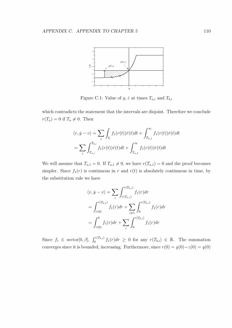
APPENDIX C. APPENDIX TO CHAPTER 5 110
5 4 3 2 1 0 1 2 3 4 5 2
1. 5
1
0. 5
0
0.5
1
1.5
2
2.5
3
z dot
y
y(Tb,i)
y(Ta,i)
Figure C.1: Value of y, z at times Ta,i and Tb,i
which contradicts the statement that the intervals are disjoint. Therefore we conclude
r(Ta) = 0 if Ta 6= 0. Then
〈v, y − v〉 =∑
i
∫
Ii
f1(r(t))r(t)dt +
∫ ∞
Ta,f
f1(r(t))r(t)dt
=∑
i
∫ Tb,i
Ta,i
f1(r(t))r(t)dt +
∫ ∞
Ta,f
f1(r(t))r(t)dt
We will assume that Ta,1 = 0. If Ta,1 6= 0, we have r(Ta,1) = 0 and the proof becomes
simpler. Since f1(r) is continuous in r and r(t) is absolutely continuous in time, by
the substitution rule we have
〈v, y − v〉 =∑
i
∫ r(Tb,i)
r(Ta,i)
f1(r)dr
=
∫ r(Tb,1)
r(0)
f1(r)dr +∑
i6=1
∫ r(Tb,i)
0
f1(r)dr
=
∫ 0
r(0)
f1(r)dr +∑
i
∫ r(Tb,i)
0
f1(r)dr
Since f1 ∈ sector[0, β],∫ r(Tb,i)
0f1(r)dr ≥ 0 for any r(Tb,i) ∈ R. The summation
converges since it is bounded, increasing. Furthermore, since r(0) = y(0)−z(0) = y(0)
APPENDIX C. APPENDIX TO CHAPTER 5 111
and | ∫ y
0f1(r)dr| ≤ f1(y)y ≤ βy2 for any y, we have
〈v, y − v〉 =
∫ 0
y(0)
f1(r)dr +∑
i
∫ r(Tb,i)
0
f1(r)dr ≥ −β|y(0)|2
Theorem 121. For any initial condition x0 ∈ W2 with x0(−τ) > −p0, x0(θ) ≥ −p0,
there exists a f ∈ W2 and T > 0 such that A(x0, t) = Bz(f, t + T ) for t ≥ 0.
Proof. Recall the map Bz is defined by the following dynamics for z = Bzy.
z(t) = 0 for t ≤ 0 and for t ≥ 0
z(t) = fc
(z(t), y(t)− z(t− τ)
)
Now suppose we let y(t) = f(t) + z(t− τ) on a finite interval [0, T ′] for some f ∈ W2.
The system is still well-posed and y ∈ W2 if f ∈ W2 since the derivative of z is
bounded. The dynamics are now given by z(t) = 0 for t ≤ 0 and the following for
t ≥ 0
z(t) = fc
(z(t), f(t)
)
Part 1: The first part of the proof is to construct a f ∈ W2 that drives the state
z(t) to z(T ′) = x0(0) for some T ′ ≥ 0. Furthermore, for continuity with Part 2, we
require that f(T ′) = −x0(−τ). If x0(−τ) = 0 and x0(0) = 0, then we are done.
Otherwise, there are 4 cases to consider.
x0(−τ) < 0, x0(0) > 0 First, let f(t) = εt until T1 = −x0(−τ)ε
for ε > 0. Let ε be
sufficiently large so that z(T1) < x0(0). Such an ε exists since z is bounded. Let
f(t) = −x0(−τ) > 0 until time T ′ such that z(T ′) = x0(0). Such T ′ exists since z(t)
is now linearly increasing.
APPENDIX C. APPENDIX TO CHAPTER 5 112
x0(−τ) > 0, x0(0) < 0 This case is handled similarly to the previous one.
x0(−τ) < 0, x0(0) < 0 For this case, let f(t) = −εt until time T1 = 1ε. Then
let f(t) = −1 until time T2 such that z(T2) = x0(0) − γ for some γ > 0. Such
time exists for any γ < p0 − x0(0) since z(t) is linearly decreasing for z(t) ≥ −p0.
Then let f(t) = x0(0) − γ + λt for time ∆t = 1λ(x0(−τ) + 1). Make λ sufficiently
large so that z(T2 + ∆t) < x0(0). This is possible since z is bounded. Finally let
f(t) = −x0(−τ) > 0 until time T ′ when z(T ′) = x0(0). Such T ′ exists since z(t) is
now linearly increasing.
x0(−τ) > 0, x0(0) > 0 or x0(0) = 0 or x0(−τ) = 0 These cases are handled simi-
larly to the previous one.
Part 2: For time t ∈ [T ′, T ′+τ ], let f(t) = −x0(t−T ′). We then have y(T ′+τ) =
x0(t−T ′)−z(T ′) = x0(−τ)−x0(−τ) = 0. Let y(t) = 0 for t ≥ T ′+τ . Therefore y ∈ W2
and we conclude that the dynamics of the interconnection for time t ∈ [T ′, T ′+ τ ] are
given by z(T ′) = x0(0)
z(t) = fc(z(t), y(t) + z(t− τ)) (C.1)
= fc(z(t), x0(t− τ)) (C.2)
And for t ≥ T ′ + τ , we have
z(t) = fc(z(t), y(t) + z(t− τ)) (C.3)
= fc(z(t),−z(t− τ)) (C.4)
Therefore, we have that A(y, t + T ′) = B(x0, t).

APPENDIX C. APPENDIX TO CHAPTER 5 113
Lemma 122. Suppose that for any δ > 0, there exists a Tδ such that T2 > T1 > Tδ
implies z(T2)2−z(T1)
2 < δ. Then for any infinite, increasing sequence, Ti, z(Ti)2
is a Cauchy sequence.
Proof. Proof by contradiction. Suppose that z(Ti)2 is not a Cauchy sequence.
Then there exists an ε > 0 such that for any N > 0, there exists i, j > N such that
|z(Ti)2 − z(Tj)
2| > ε.
Let δ = ε2. By assumption there exists a Tδ such that for all T2 > T1 > Tδ,
z(T2)2 − z(T1)
2 <ε
2(C.5)
Since Ti is strictly increasing, infinite, there exists a N > 0 such that TN > Tδ.
Since z(Ti)2 is not Cauchy, there exists i1, j1 > N such that |z(Ti1)
2− z(Tj1)2| > ε.
Without loss of generality, we may assume i1 > j1. We now have one of the two
possibilities.
• z(Ti1)2 − z(Tj1)
2 > ε
• z(Ti1)2 − z(Tj1)
2 < −ε
However, by Equation (C.5), the first option is not possible since Ti > Tj > TN > Tδ.
Therefore z(Ti1)2 < z(Tj1)
2 − ε. Thus for all k > i1, by (C.5) and since Tk > Ti1 >
Tj1 > TN ≥ Tδ, we have
z(Tk)2 < z(Ti1)
2 +ε
2< z(Tj1)
2 − ε +ε
2= z(Tj1)
2 − ε
2
Now, let N = i1. Again, since z(Ti)2 is not Cauchy, there exists i2, j2 > i1
such that |z(Ti2)2 − z(Tj2)
2| > ε. Using the method above, for all k > i2 since
Tk > Ti2 > Tj2 > Ti1 > Tδ, by (C.5) we have
z(Tk)2 < z(Ti2)
2 +ε
2< z(Tj2)
2 − ε
2< z(Tj1)
2 − 2ε
2
Repeating n times, we find a in such that for all k > in, z(Tk)2 < z(Tj1)
2 − n ε2.
Since we can assume z(Tj1)2 is finite, let n be sufficiently large and we have the
APPENDIX C. APPENDIX TO CHAPTER 5 114
existence of an i such that that z(Ti)2 < 0, which is a contradiction. Thus we have
that z(Ti)2 is a Cauchy sequence.

Appendix D
Appendix to Chapter 7
Theorem 123. Suppose M : R→ S2n is a continuous matrix-valued function. Then
the following are equivalent
1. There exists some ε > 0 such that the following holds for all x ∈ Cτ .
∫ 0
−τ
[x(0)
x(θ)
]T
M(θ)
[x(0)
x(θ)
]dθ ≥ ε‖x‖2
2
2. There exists some ε′ > 0 and some continuous matrix-valued function T : R→Sn such that the following holds.
∫ 0
−τ
T (θ)dθ = 0
M(θ) +
[T (θ) 0
0 −ε′I
]≥ 0 for all θ ∈ [−τ, 0]
115
APPENDIX D. APPENDIX TO CHAPTER 7 116
Proof. (2 ⇒ 1) Suppose statement 2 is true, then
∫ 0
−τ
[x(0)
x(θ)
]T
M(θ)
[x(0)
x(θ)
]dθ − ε′‖x‖2
2
=
∫ 0
−τ
[x(0)
x(θ)
]T
M(θ) +
[T (θ) 0
0 −ε′I
][x(0)
x(θ)
]dθ ≥ 0.
(1 ⇒ 2) Suppose that statement 1 holds for some M . Write M as
M(θ) =
[M11(θ) M12(θ)
M12(θ)T M22(θ)
].
We first prove that M22(θ) ≥ εI for all θ ∈ [−τ, 0]. By statement 1, we have that
∫ 0
−τ
[x(0)
x(θ)
]T [M11(θ) M12(θ)
M12(θ)T M22(θ)− εI
][x(0)
x(θ)
]dθ ≥ 0.
Now suppose that M22(θ) − εI is not positive semidefinite for all θ ∈ [−τ, 0]. Then
there exists some x0 ∈ Rn and θ1 ∈ [−τ, 0] such that xT0 (M22(θ1) − εI)x0 < 0.
By continuity of M22, if θ1 = 0 or θ1 = −τ , then there exists some θ′1 ∈ (−τ, 0)
such that xT0 (M22(θ
′1) − εI)x0 < 0. Thus assume θ1 ∈ (−τ, 0). Now, since M22
is continuous, there exists some x1 and δ > 0 where θ1 + δ < 0, θ1 − δ > −τ
and such that xT1 (M22(θ) − εI)x1 ≤ −1 for all θ ∈ [θ1 − δ, θ1 + δ]. Then for β >
max1/(−θ1 − δ), 1/(τ + θ1 − δ), let
x(θ) =
(1 + β(θ − (θ1 − δ)))x1 θ ∈ [θ1 − δ − 1/β, θ1 − δ]
x1 θ ∈ [θ1 − δ, θ1 + δ]
(1− β(θ − (θ1 + δ)))x1 θ ∈ [θ1 + δ, θ1 + δ + 1/β]
0 otherwise.
Then x ∈ Cτ , x(0) = 0 and ‖x(θ)‖ ≤ ‖x1‖ for all θ ∈ [−τ, 0]. Now, since M22 is
continuous, it is bounded on [−τ, 0]. Therefore, there exists some ε2 > 0 such that

APPENDIX D. APPENDIX TO CHAPTER 7 117
M22(θ)− εI ≤ ε2I. Then let β ≥ 2ε2‖x1‖2/δ and we have the following.
∫ 0
−τ
[x(0)
x(θ)
]T
M(θ)
[x(0)
x(θ)
]dθ − ε‖x‖2
=
∫ 0
−τ
x(θ)T (M22(θ)− εI)x(θ)dθ
=
∫ θ1+δ
θ1−δ
xT1 (M22(θ)− εI)x1dθ
+
∫ θ1−δ
θ1−δ−1/β
x(θ)T (M22(θ)− εI)x(θ)dθ
+
∫ θ1+δ+1/β
θ1+δ
x(θ)T (M22(θ)− εI)x(θ)dθ
≤ −2δ + ε2
∫ θ1−δ
θ1−δ−1/β
‖x(θ)‖2dθ + ε2
∫ θ1+δ+1/β
θ1+δ
‖x(θ)‖2dθ
≤ −2δ + 2ε2‖x1‖2/β ≤ −δ
Therefore, by contradiction, we have that M22(θ) ≥ εI for all θ ∈ [−τ, 0]. Now we
define ε′ = ε/2 and M22(θ) = M22(θ) − ε′I ≥ ε′I. We now show that M22(θ)−1 is
continuous. We first note that M22(θ)−1 is bounded, since
M22(θ) ≥ ε′I ⇒ I ≥ ε′M22(θ)−1 ⇒ M22(θ)
−1 ≤ 1
ε′I
Now since M22 is continuous, for any β > 0, there exists a δ > 0 such that
|θ1 − θ2| ≤ δ ⇒ ‖M22(θ1)− M22(θ2)‖ ≤ β

APPENDIX D. APPENDIX TO CHAPTER 7 118
Therefore, for any β′ > 0, let δ be defined as above for β = β′ε′2. Then |θ1 − θ2| ≤ δ
implies
‖M22(θ1)−1 − M22(θ2)
−1‖= ‖M22(θ1)
−1M22(θ2)M22(θ2)−1 − M22(θ1)
−1M22(θ1)M22(θ2)−1‖
= ‖M22(θ1)−1
(M22(θ2)− M22(θ1)
)M22(θ2)
−1‖
≤ ‖M22(θ1)−1‖‖M22(θ2)− M22(θ1)‖‖M22(θ2)
−1‖ ≤ 1
ε′2‖M22(θ2)− M22(θ1)‖ ≤ β′.
Therefore M22(θ)−1 is continuous. We now prove statement 2 by construction. Sup-
pose M satisfies statement 1. Let
T (θ) = T0 − (M11(θ)−M12(θ)M−122 (θ)M12(θ)
T ).
Here
T0 =1
τ
∫ 0
−τ
(M11(θ)−M12(θ)M−122 (θ)M12(θ)
T )dθ.
Then we have that T is continuous and
∫ 0
−τ
T (θ)dθ = τT0 − τT0 = 0.
This implies that T ∈ Ω. We now prove that T0 ≥ 0. For any vector z0 ∈ Rn,
suppose z is a continuous function such that z(0) = (I + M22(0)−1M12(0)T )z0. Then
let x(θ) = z(θ) − M22(θ)−1M12(θ)
T z0. Then x is continuous, x(0) = z0 and by

APPENDIX D. APPENDIX TO CHAPTER 7 119
statement 1 we have the following.
∫ 0
−τ
[x(0)
x(θ)
]T [M11(θ) M12(θ)
M12(θ)T M22(θ)
][x(0)
x(θ)
]dθ
=
∫ 0
−τ
[z0
z(θ)
]T [I 0
−M22(θ)−1M12(θ)
T I
]T [M11(θ) M12(θ)
M12(θ)T M22(θ)
]
[I 0
−M22(θ)−1M12(θ)
T I
][z0
z(θ)
]dθ
=
∫ 0
−τ
[z0
z(θ)
]T [M11(θ)−M12(θ)M
−122 (θ)M12(θ)
T 0
0 M22(θ)
][z0
z(θ)
]dθ
= zT0 (
∫ 0
−τ
M11(θ)−M12(θ)M−122 (θ)M12(θ)
T dθ)z0
+
∫ 0
−τ
z(θ)T M22(θ)z(θ)dθ
= zT0 T0z0 +
∫ 0
−τ
z(θ)T M22(θ)z(θ)dθ ≥ ε′‖x‖22
We now show that this implies that T0 ≥ 0. Suppose there exists some y such that
yT T0y < 0. Then there exists some z0 such that z0T0z0 = −1. Now let α > 1/τ and
z(θ) =
(I + M22(0)−1M12(0)T )z0(1 + αθ) θ ∈ [−1/α, 0]
0 otherwise.
Then z is continuous, z(0) = (I + M22(0)−1M12(0)T )z0 and ‖z(θ)‖2 ≤ ‖z(0)‖2 for all
θ ∈ [−τ, 0]. Recall that M22(θ) ≤ (ε2 + ε′)I = ε3I. Let α > 2ε3‖z(0)2‖ and then we
have the following.
zT0 T0z0 +
∫ 0
−τ
z(θ)T M22(θ)z(θ)dθ ≤ −1 + ε3
∫ 0
−1/α
‖z(θ)‖2
≤ −1 + ε3‖z(0)‖2/α < −1
2

APPENDIX D. APPENDIX TO CHAPTER 7 120
However, this contradicts the previous relationship. Therefore, we have by contradic-
tion that T0 ≥ 0. Now by using the invertibility of M22(θ) = M22(θ)− ε′I ≥ ε′I and
the Schur complement transformation, we have that statement 2 is equivalent to the
following for all θ ∈ [−τ, 0].
M22(θ) ≥ 0
M11(θ) + T (θ)−M12(θ)M22(θ)−1M12(θ)
T ≥ 0
We have already proven the first condition. Finally, we have the following.
M11(θ) + T (θ)−M12(θ)M22(θ)−1M12(θ)
T = T0 ≥ 0
Thus we have shown that statement 2 is true.
Lemma 124. Let M : R 7→ S3n be a continuous matrix-valued function. Then the
following are equivalent.
1. There exists an ε > 0 such that the following holds for all x ∈ Cτ .
∫ 0
−τ
x(0)
x(−τ)
x(θ)
T
M(θ)
x(0)
x(−τ)
x(θ)
≥ ε‖x‖2
2
2. There exists some ε′ > 0 and a continuous matrix valued function T : R 7→ S2n
such that the following holds.
∫ 0
−τ
T (θ)dθ = 0
M(θ) +
[T (θ) 0
0 −ε′I
]≥ 0 for all θ ∈ [−τ, 0]

APPENDIX D. APPENDIX TO CHAPTER 7 121
Proof. (2 ⇒ 1) Suppose there exists some function T ∈ S0 such that
M(θ) +
[T (θ) 0
0 −ε′I
]≥ 0 for all θ ∈ [−τ, 0].
Then we have the following.
∫ 0
−τ
x(0)
x(−τ)
x(θ)
T
M(θ)
x(0)
x(−τ)
x(θ)
dθ − ε′‖x‖2
2
=
∫ 0
−τ
x(0)
x(−τ)
x(θ)
T
M(θ) +
[T (θ) 0
0 −ε′I
]
x(0)
x(−τ)
x(θ)
dθ ≥ 0
(1 ⇒ 2) Suppose that statement 1 holds for some M . Write M as
M(θ) =
[M11(θ) M12(θ)
M12(θ)T M22(θ)
],
where M22 : R 7→ Sn. We first prove that M22(θ) ≥ εI for all θ ∈ [−τ, 0]. By
statement 1, we have that
∫ 0
−τ
x(0)
x(−τ)
x(θ)
T [M11(θ) M12(θ)
M12(θ)T M22(θ)− εI
]
x(0)
x(−τ)
x(θ)
dθ ≥ 0.
Now suppose that M22(θ) − εI is not positive semidefinite for all θ ∈ [−τ, 0]. Then
there exists some x0 and θ1 ∈ [−τ, 0] such that xT0 (M22(θ1) − εI)x0 < 0. By
continuity of M22, if θ1 = 0 or θ1 = −τ , then there exists some θ′1 ∈ (−τ, 0)
such that xT0 (M22(θ
′1) − εI)x0 < 0. Thus assume θ1 ∈ (−τ, 0). Now, since M22
is continuous, there exists some x1 and δ > 0 where θ1 + δ < 0, θ1 − δ > −τ
and such that xT1 (M22(θ) − εI)x1 ≤ −1 for θ ∈ [θ1 − δ, θ1 + δ]. Then for β >
APPENDIX D. APPENDIX TO CHAPTER 7 122
max1/(−θ1 − δ), 1/(τ + θ1 − δ), let
x(θ) =
β(θ − (θ1 − δ − 1/β))x1 θ ∈ [θ1 − δ − 1/β, θ1 − δ]
x1 θ ∈ [θ1 − δ, θ1 + δ]
(1− β(θ − (θ1 + δ)))x1 θ ∈ [θ1 + δ, θ1 + δ + 1/β]
0 otherwise.
Then x ∈ Cτ , x(−τ) = x(0) = 0 and ‖x(θ)‖2 ≤ ‖x1‖2 for all θ ∈ [−τ, 0]. Now,
since M22 is continuous, it is bounded on [−τ, 0]. Therefore, there exists some ε2 > 0
such that M22(θ) − εI ≤ ε2I for θ ∈ [−τ, 0]. Let β ≥ 2ε2‖x1‖2/δ and we have the
following.
∫ 0
−τ
x(0)
x(−τ)
x(θ)
T
M(θ)
x(0)
x(−τ)
x(θ)
dθ − ε‖x‖2
=
∫ 0
−τ
x(θ)T (M22(θ)− εI)x(θ)dθ
=
∫ θ1+δ
θ1−δ
xT1 (M22(θ)− εI)x1dθ +
∫ θ1−δ
θ1−δ−1/β
x(θ)T (M22(θ)− εI)x(θ)dθ
+
∫ θ1+δ+1/β
θ1+δ
x(θ)T (M22(θ)− εI)x(θ)dθ
≤ −2δ + ε2
∫ θ1−δ
θ1−δ−1/β
‖x(θ)‖2dθ + ε2
∫ θ1+δ+1/β
θ1+δ
‖x(θ)‖2dθ
≤ −2δ + 2ε2‖x1‖2/β ≤ −δ
Therefore, by contradiction, we have that M22(θ) ≥ εI for all θ ∈ [−τ, 0]. Now we
define ε′ = ε/2 and M22(θ) = M22(θ) − ε′I ≥ ε′I. We now show that M22(θ)−1 is

APPENDIX D. APPENDIX TO CHAPTER 7 123
continuous. We first note that M22(θ)−1 is bounded, since
M22(θ) ≥ ε′I
⇒ I ≥ ε′M22(θ)−1
⇒ M22(θ)−1 ≤ 1
ε′I
Now since M22 is continuous, for any β > 0, there exists a δ > 0 such that
|θ1 − θ2| ≤ δ ⇒ ‖M22(θ1)− M22(θ2)‖ ≤ β.
Therefore, for any β′ > 0, let δ be defined as above for β = β′ε′2. Then |θ1 − θ2| ≤ δ
implies
‖M22(θ1)−1 − M22(θ2)
−1‖= ‖M22(θ1)
−1M22(θ2)M22(θ2)−1 − M22(θ1)
−1M22(θ1)M22(θ2)−1‖
= ‖M22(θ1)−1
(M22(θ2)− M22(θ1)
)M22(θ2)
−1‖≤ ‖M22(θ1)
−1‖‖M22(θ2)− M22(θ1)‖‖M22(θ2)−1‖
≤ 1
ε′2‖M22(θ2)− M22(θ1)‖ ≤ β′.
Therefore M22(θ)−1 is continuous.
We now prove statement 2 by construction. Suppose M satisfies statement 1. Let
T (θ) = T0 − (M11(θ)−M12(θ)M−122 (θ)M12(θ)
T )
Where
T0 =1
τ
∫ 0
−τ
(M11(θ)−M12(θ)M−122 (θ)M12(θ)
T )dθ
Then we have that T is continuous and
∫ 0
−τ
T (θ)dθ = τT0 − τT0 = 0
APPENDIX D. APPENDIX TO CHAPTER 7 124
Which implies that T ∈ Ω. We now show that T0 ≥ 0. For any constant vector
z0 =[z1 z2
]T
, suppose that z is a continuous function such that
z(0) = z1 + M22(0)−1M12(0)T z0
z(−τ) = z2 + M22(−τ)−1M12(−τ)T z0.
Then, let x(θ) = z(θ)−M22(θ)−1M12(θ)
T z0. Then x is continuous,[x(0) x(−τ)
]T
=
z0 and by statement 1 we have the following.
∫ 0
−τ
x(0)
x(−τ)
x(θ)
T [M11(θ) M12(θ)
M12(θ)T M22(θ)
]
x(0)
x(−τ)
x(θ)
dθ
=
∫ 0
−τ
[z0
z(θ)
]T [I 0
−M22(θ)−1M12(θ)
T I
]T [M11(θ) M12(θ)
M12(θ)T M22(θ)
]
[I 0
−M22(θ)−1M12(θ)
T I
][z0
z(θ)
]dθ
=
∫ 0
−τ
[z0
z(θ)
]T [M11(θ)−M12(θ)M
−122 (θ)M12(θ)
T 0
0 M22(θ)
][z0
z(θ)
]dθ
= zT0 (
∫ 0
−τ
M11(θ)−M12(θ)M−122 (θ)M12(θ)
T dθ)z0 +
∫ 0
−τ
z(θ)T M22(θ)z(θ)dθ
= zT0 T0z0 +
∫ 0
−τ
z(θ)T M22(θ)z(θ)dθ ≥ ε′‖x‖22
We now show that this implies that T0 ≥ 0. Suppose there exists some y such that
yT T0y < 0. Then there exists some z0 such that z0T0z0 = −1. Now let z0 =[z1 z2
]T
,

APPENDIX D. APPENDIX TO CHAPTER 7 125
c1 = z1 + M22(0)−1M12(0)T z0, c2 = z2 + M22(−τ)−1M12(−τ)T z0, α > 2/τ and
z(θ) =
c1(1 + αθ) θ ∈ [−1/α, 0]
c2(1− (θ + τ)α) θ ∈ [−τ,−τ + 1/α]
0 otherwise
.
Then z is continuous, z(0) = c1 = z1 + M22(0)−1M12(0)T z0, z(−τ) = c2 = z2 +
M22(−τ)−1M12(−τ)T z0, and ‖z(θ)‖2 ≤ c = max‖c1‖2, ‖c2‖2 for all θ ∈ [−τ, 0].
Recall that M22(θ) ≤ (ε2 + ε′)I = ε3I. Let α > 2ε3c and then we have
zT0 T0z0 +
∫ 0
−τ
z(θ)T M22(θ)z(θ)dθ ≤ −1 + ε3
∫ 0
−1/α
‖z(θ)‖2
≤ −1 + ε3c/α < −1
2.
This contradicts the previous statement. Thus we have by contradiction that
T0 ≥ 0. Now by using the invertibility of M22 = M22(θ) − ε′I ≥ ε′I and the Schur
complement transformation, we have that statement 2 is equivalent to the following.
M22(θ) ≥ 0
M11(θ) + T (θ)−M12(θ)M22(θ)−1M12(θ)
T ≥ 0
The first condition has already been proven. Finally, we have the following.
M11(θ) + T (θ)−M12(θ)M22(θ)−1M12(θ)
T = T0 ≥ 0
Thus we have shown that statement 2 is true.
Lemma 125. Suppose M is a matrix valued function which is continuous except
possibly at points τiK−1i=1 where τi ∈ [−τK , 0]. Then the following are equivalent.

APPENDIX D. APPENDIX TO CHAPTER 7 126
1. The following holds for all x ∈ CτK.
∫ 0
−τK
[x(0)
x(θ)
]T
M(θ)
[x(0)
x(θ)
]≥ 0
2. The following holds for all x where x is continuous except possibly at points
−τiK−1i=1 .
∫ 0
−τK
[x(0)
x(θ)
]T
M(θ)
[x(0)
x(θ)
]≥ 0
Proof. Clearly statement 2 implies statement 1. Now suppose statement 2 is false.
Then there exists some piecewise continuous x , ε > 0 such that
V1 =
∫ 0
−τK
[x(0)
x(θ)
]M(θ)
[x(0)
x(θ)
]dθ ≤ −ε.
Now let
x(θ)
=
x(−τi − 1β)+(x(−τi + 1
β)−x(−τi − 1
β))(β(θ + τi + 1
β)/2)
θ∈[−τi − 1β,−τi + 1
β],
i = 1, . . . , K − 1
x(θ) otherwise.
Then x is continuous. Since x is piecewise continuous on [−τK , 0], it is bounded on
this interval. Now let c = maxθ∈[−τK ,0] ‖x(θ)‖2. Then ‖x(θ)‖2 ≤ c for all θ ∈ [−τk, 0].
Now since M is piecewise continuous on [−τk, 0], there exists some ε′ > 0 such that

APPENDIX D. APPENDIX TO CHAPTER 7 127
M(θ) < ε′I for θ ∈ [−τk, 0]. Therefore we have the following.
∫ 0
−τ
[x(0)
x(θ)
]T
M(θ)
[x(0)
x(θ)
]dθ
= V1 +K−1∑i=1
∫ −τi+1/β
−τi−1/β
([x(0)
x(θ)
]M(θ)
[x(0)
x(θ)
]−
[x(0)
x(θ)
]M(θ)
[x(0)
x(θ)
])dθ
≤ V1 +K−1∑i=1
∫ −τi+1/β
−τi−1/β
ε′((‖x(θ)‖2 + ‖x(0)‖2
)+
(‖x(θ)‖2 + ‖x(0)‖2))
dθ
≤ V1 + 2ε′(K − 1)(4c)/β
≤ −ε + 8ε′(K − 1)c/β
≤ −ε/2
Which holds for β ≥ 16ε′(K−1)cε
. Thus statement 2 is false implies statement 1 is false.
Therefore statement 1 implies statement 2.
Lemma 126. Suppose Si : R 7→ S2n, i = 1 . . . K are continuous symmetric matrix
valued functions with domains [−τi,−τi−1] where τK > τi > τi−1 > τ0 = 0 for i =
2 . . . K − 1. Then the following are equivalent.
1. There exists an ε > 0 such that the following holds for all x ∈ CτK.
K∑i=1
∫ −τi−1
−τi
[x(0)
x(θ)
]Si(θ)
[x(0)
x(θ)
]dθ ≥ ε‖x‖2
2
2. There exists an ε′ > 0 and continuous symmetric matrix valued functions, Ti :
R 7→ Sn, such that
Si(θ) +
[Ti(θ) 0
0 −ε′I
]≥ 0 for θ ∈ [−τi,−τi−1] i = 1 . . . K
K∑i=1
∫ −τi−1
−τi
Ti(θ) = 0.
APPENDIX D. APPENDIX TO CHAPTER 7 128
Proof. (2 ⇒ 1) Suppose there exist continuous symmetric matrix valued functions,
Ti : R 7→ Sn, such that
Si(θ) +
[Ti(θ) 0
0 −ε′I
]≥ 0 i = 1 . . . K
K∑i=1
∫ −τi−1
−τi
Ti(θ) = 0.
Then
K∑i=1
∫ −τi−1
−τi
[x(0)
x(θ)
]Si(θ)
[x(0)
x(θ)
]dθ − ε′‖x‖2
2
=K∑
i=1
∫ −τi−1
−τi
[x(0)
x(θ)
]Si(θ) +
[Ti(θ) 0
0 −ε′I
][x(0)
x(θ)
]dθ ≥ 0.
(1 ⇒ 2) Suppose that statement 1 holds for some Si. Write Si as
Si(θ) =
[M11i(θ) M12i(θ)
M12i(θ)T M22i(θ)
].
We first prove that M22i(θ) ≥ εI for all θ ∈ [−τi,−τi−1], i = 1, . . . , K. By
statement 1, we have that
K∑i=1
∫ −τi−1
−τi
[x(0)
x(θ)
][M11i(θ) M12i(θ)
M12i(θ)T M22i(θ)− εI
][x(0)
x(θ)
]dθ ≥ 0.
Now suppose that M22i(θ) − εI is not positive semidefinite for all θ ∈ [−τi,−τi−1].
Then there exists some x0 ∈ Rn and θ1 ∈ [−τi,−τi−1] such that xT0 (M22i(θ1) −
εI)x0 < 0. By continuity of M22i, if θ1 = −τi or θ1 = −τi−1, then there exists some
θ′1 ∈ (−τi,−τi−1) such that xT0 (M22i(θ
′1)− εI)x0 < 0. Thus assume θ1 ∈ (−τi,−τi−1).
Now, since M22i is continuous, there exists some x1 and δ > 0 where θ1 + δ < −τi−1,
θ1− δ > −τi and such that xT1 (M22i(θ)− εI)x1 ≤ −1 for θ ∈ [θ1− δ, θ1 + δ]. Then for

APPENDIX D. APPENDIX TO CHAPTER 7 129
β > max1/(−τi − θ1 − δ), 1/(τi + θ1 − δ), let
x(θ) =
β(θ − (θ1 − δ − 1/β))x1 θ ∈ [θ1 − δ − 1/β, θ1 − δ]
x1 θ ∈ [θ1 − δ, θ1 + δ]
(1− β(θ − (θ1 + δ)))x1 θ ∈ [θ1 + δ, θ1 + δ + 1/β]
0 otherwise.
Then x ∈ CτK, x(0) = 0 and ‖x(θ)‖2 ≤ ‖x1‖2 for θ ∈ [−τK , 0]. Now, since every
M22i is continuous, they are bounded on [−τi,−τi−1]. Therefore, there exists some
ε2 > 0 such that M22i(θ) − εI ≤ ε2I for θ ∈ [−τi,−τi−1], i = 1, . . . , K. Then let
β ≥ 2ε2‖x1‖2/δ and we have the following.
K∑j=1
∫ −τj−1
−τj
[x(0)
x(θ)
]T
Sj(θ)
[x(0)
x(θ)
]dθ − ε‖x‖2 =
K∑j=1
∫ −τj−1
−τj
x(θ)T (M22j(θ)− εI)x(θ)dθ
=
∫ θ1+δ
θ1−δ
xT1 (M22i(θ)− εI)x1dθ +
∫ θ1−δ
θ1−δ−1/β
x(θ)T (M22i(θ)− εI)x(θ)dθ
+
∫ θ1+δ+1/β
θ1+δ
x(θ)T (M22i(θ)− εI)x(θ)dθ
≤ −2δ + ε2
∫ θ1−δ
θ1−δ−1/β
‖x(θ)‖2dθ + ε2
∫ θ1+δ+1/β
θ1+δ
‖x(θ)‖2dθ
≤ −2δ + 2ε2‖x1‖2/β ≤ −δ
Therefore, by contradiction, we have that M22i(θ) ≥ εI for all θ ∈ [−τi,−τi−1] and
i = 1, . . . , K. Now we define ε′ = ε/2 and M22i(θ) = M22i(θ) − ε′I ≥ ε′I. We now
show that M22i(θ)−1 is continuous. We first note that M22i(θ)
−1 is bounded, since
M22i(θ) ≥ ε′I
⇒ I ≥ ε′M22i(θ)−1
⇒ M22i(θ)−1 ≤ 1
ε′I.

APPENDIX D. APPENDIX TO CHAPTER 7 130
Now since M22i is continuous, for any β > 0, there exists a δ > 0 such that
|θ1 − θ2| ≤ δ ⇒ ‖M22i(θ1)− M22i(θ2)‖ ≤ β.
Therefore, for any β′ > 0, let δ be defined as above for β = β′ε′2. Then |θ1 − θ2| ≤ δ
implies the following.
‖M22i(θ1)−1 − M22i(θ2)
−1‖= ‖M22i(θ1)
−1M22i(θ2)M22i(θ2)−1 − M22i(θ1)
−1M22i(θ1)M22i(θ2)−1‖
= ‖M22i(θ1)−1
(M22i(θ2)− M22i(θ1)
)M22i(θ2)
−1‖≤ ‖M22i(θ1)
−1‖‖M22i(θ2)− M22i(θ1)‖‖M22i(θ2)−1‖
≤ 1
ε′2‖M22i(θ2)− M22i(θ1)‖ ≤ β′
Therefore M22i(θ)−1 is continuous.
We now prove statement 2 by construction. Let
Ti(θ) = T0 − (M11i(θ)−M12i(θ)M−122i(θ)M12i(θ)
T ),
where
T0 =1
τK
K∑i=1
∫ −τi−1
−τi
(M11i(θ)−M12i(θ)M−122i(θ)M12i(θ)
T )dθ.
Then we have that Ti is continuous and
K∑i=1
∫ −τi−1
−τi
Ti(θ)dθ = τKT0 − τKT0 = 0.
We now show that T0 ≥ 0. For any constant vector z0, let z be a continuous function
except possibly at points −τiK−1i=1 and such that z(0) = (I + M221(0)−1M121(0)T )z0,
let x(θ) = z(θ) − M22i(θ)−1M12i(θ)
T z0 for θ ∈ [−τi,−τi−1]. Then x is continuous
except possibly at points −τiK−1i=1 , x(0) = z0 and by statement 1, and Lemma 125
we have the following.

APPENDIX D. APPENDIX TO CHAPTER 7 131
K∑i=1
∫ −τi−1
−τi
[x(0)
x(θ)
]T [M11i(θ) M12i(θ)
M12i(θ)T M22i(θ)
][x(0)
x(θ)
]dθ
=K∑
i=1
∫ −τi−1
−τi
[z0
z(θ)
]T [I 0
−M22i(θ)−1M12i(θ)
T I
]T [M11i(θ) M12i(θ)
M12i(θ)T M22i(θ)
]
[I 0
−M22i(θ)−1M12i(θ)
T I
][z0
z(θ)
]dθ
=K∑
i=1
∫ −τi−1
−τi
[z0
z(θ)
]T [M11i(θ)−M12i(θ)M
−122i(θ)M12i(θ)
T 0
0 M22i(θ)
][z0
z(θ)
]dθ
= zT0
( K∑i=1
∫ −τi−1
−τi
M11i(θ)−M12i(θ)M−122i(θ)M12i(θ)
T dθ
)z0+
K∑i=1
∫ −τi−1
−τi
z(θ)T M22i(θ)z(θ)dθ
= zT0 T0z0 +
K∑i=1
∫ −τi−1
−τi
z(θ)T M22i(θ)z(θ)dθ ≥ ε′‖x‖22
We now show that this implies that T0 ≥ 0. Suppose there exists some y such
that yT T0y < 0. Then there exists some z0 such that z0T0z0 = −1. Now let α > 1/τ1
and
z(θ) =
(I + M221(0)−1M121(0)T )z0(1 + αθ) θ ∈ [−1/α, 0]
0 otherwise.
Then z is continuous, z(0) = (I + M221(0)−1M121(0)T )z0 and ‖z(θ)‖2 ≤ ‖z(0)‖2 for
all θ ∈ [−τ, 0]. Recall that M22i(θ) ≤ (ε2 + ε′)I = ε3I. Let α > 2ε3‖z(0)2‖ and then
we have
zT0 T0z0 +
K∑i=1
∫ −τi−1
−τi
z(θ)T M22i(θ)z(θ)dθ ≤ −1 + ε3
∫ 0
−1/α
‖z(θ)‖2
≤ −1 + ε3‖z(0)‖2/α < −1
2.
But this is in contradiction to the previous relation. Thus we have by contradiction
that T0 ≥ 0. Now by using the invertibility of M22i = M22i(θ)−ε′I ≥ ε′I and the Schur

APPENDIX D. APPENDIX TO CHAPTER 7 132
complement transformation, we have that statement 2 is equivalent to the following
for i = 1, . . . , K.
M22i(θ) ≥ 0 θ ∈ [−τi,−τi−1]
M11i(θ) + Ti(θ)−M12i(θ)M22i(θ)−1M12i(θ)
T ≥ 0 θ ∈ [−τi,−τi−1]
We have already shown the first statement. Finally, we have the following for i =
1 . . . K.
M11i(θ) + Ti(θ)−M12i(θ)M22i(θ)−1M12i(θ)
T = T0 ≥ 0
Thus we have shown that statement 2 is true.
Lemma 127. Suppose MiKi=1 are continuous symmetric matrix valued functions
with domains [−τi,−τi−1] and τK > τi > τi−1 > τ0 = 0 for i = 2 . . . K − 1. Then the
following are equivalent.
1. The following holds for all x ∈ CτK.
K∑i=1
∫ −τi−1
−τi
x(−τ0)...
x(−τK)
x(θ)
T
Mi(θ)
x(−τ0)...
x(−τK)
x(θ)
dθ ≥ 0
2. The following holds for all x where x is continuous except possibly at points
−τiK−1i=1 .
K∑i=1
∫ −τi−1
−τi
x(−τ0)−
x(−τ1)+
...
x(−τK)+
x(θ)
T
Mi(θ)
x(−τ0)−
x(−τ1)+
...
x(−τK)+
x(θ)
dθ ≥ 0

APPENDIX D. APPENDIX TO CHAPTER 7 133
Where x(τ)− denotes the left-handed limit and x(τ)+ denotes the right-handed
limit.
Proof. Clearly statement 2 implies statement 1. Now suppose statement 2 is false.
Then there exists some piecewise continuous x , and ε > 0 such that
V1 =K∑
i=1
∫ −τi−1
−τi
x(−τ0)−
x(−τ1)+
...
x(−τK)+
x(θ)
T
Mi(θ)
x(−τ0)−
x(−τ1)+
...
x(−τK)+
x(θ)
dθ ≤ −ε.
Now let β > maxi=1,...,K2/(τi − τi−1) and
x(θ) =
x(−τi − 1β) + (x(−τi)
+ − x(−τi − 1β))β(θ + τi + 1
β)
θ ∈ [−τi − 1β,−τi],
i = 1, . . . , K − 1
x(θ) otherwise.
Then x is continuous on [−τK , 0], x(0) = x(0)− and x(−τi) = x(−τi)+ for i =
1, . . . , K. Since x is piecewise continuous on [−τK , 0], it is bounded on this interval.
Now let c = maxθ∈[−τK ,0] ‖x(θ)‖2. Then ‖x(θ)‖2 ≤ c for all θ ∈ [−τk, 0]. Now since
M is piecewise continuous on [−τk, 0], there exists some ε′ > 0 such that M(θ) < ε′I

APPENDIX D. APPENDIX TO CHAPTER 7 134
for θ ∈ [−τk, 0]. Therefore we have the following.
K∑i=1
∫ −τi−1
−τi
x(−τ0)...
x(−τK)
x(θ)
T
Mi(θ)
x(−τ0)...
x(−τK)
x(θ)
dθ
=K∑
i=1
∫ −τi−1
−τi
x(−τ0)−
x(−τ1)+
...
x(−τK)+
x(θ)
T
Mi(θ)
x(−τ0)−
x(−τ1)+
...
x(−τK)+
x(θ)
dθ
= V1 +K−1∑i=1
∫ −τi
−τi−1/β
(
x(−τ0)−
x(−τ1)+
...
x(−τK)+
x(θ)
T
Mi+1(θ)
x(−τ0)−
x(−τ1)+
...
x(−τK)+
x(θ)
−
x(−τ0)−
x(−τ1)+
...
x(−τK)+
x(θ)
T
Mi+1(θ)
x(−τ0)−
x(−τ1)+
...
x(−τK)+
x(θ)
)dθ
≤ V1 +K−1∑i=1
∫ −τi
−τi−1/β
ε′((
‖x(θ)‖2+K∑
j=0
‖x(−τj)‖2
)+
(‖x(θ)‖2 +
K∑j=0
‖x(−τj)‖2
))dθ
≤ V1 + ε′(K − 1)(2c + 2(K + 1)c)/β
≤ −ε + 2ε′(K − 1)(K + 2)/β
≤ −ε/2
Which holds for β ≥ 4ε′(K−1)(K+2)ε
. Thus statement 2 is false implies statement 1 is
false. Therefore statement 1 implies statement 2.
APPENDIX D. APPENDIX TO CHAPTER 7 135
Lemma 128. Suppose Si : R 7→ Sn(K+2) are continuous matrix valued functions
with domains [−τi,−τi−1] for i = 1, . . . , K where τK > τi > τi−1 > τ0 = 0 for
i = 2, . . . , K − 1. Then the following are equivalent.
1. There exists an ε > 0 such that the following holds for all x ∈ CτK.
K∑i=1
∫ −τi−1
−τi
x(−τ0)...
x(−τK)
x(θ)
T
Si(θ)
x(−τ0)...
x(−τK)
x(θ)
dθ ≥ ε‖x‖22
2. There exists an ε′ > 0 and continuous matrix valued functions Ti : R 7→ Sn(K+1)
such that
Si(θ) +
[Ti(θ) 0
0 −ε′I
]≥ 0 θ ∈ [−τi,−τi−1], i = 1 . . . K
K∑i=1
∫ −τi−1
−τi
Ti(θ) = 0.
Proof. (2 ⇒ 1) Suppose there exist continuous symmetric matrix valued functions,
Ti : R 7→ Sn(K+1), such that
Si(θ) +
[Ti(θ) 0
0 −ε′I
]≥ 0 i = 1 . . . K
K∑i=1
∫ −τi−1
−τi
Ti(θ) = 0.
Then
APPENDIX D. APPENDIX TO CHAPTER 7 136
K∑i=1
∫ −τi−1
−τi
x(−τ0)...
x(−τK)
x(θ)
T
Si(θ)
x(−τ0)...
x(−τK)
x(θ)
dθ − ε‖x‖22
=K∑
i=1
∫ −τi−1
−τi
x(−τ0)...
x(−τK)
x(θ)
T
Si(θ)−[Ti(θ) 0
0 −ε′I
]
x(−τ0)...
x(−τK)
x(θ)
dθ ≥ 0.
(1 ⇒ 2) Suppose that statement 1 holds for some Si. Write Si as
Si(θ) =
[M11i(θ) M12i(θ)
M12i(θ)T M22i(θ)
],
where M22i : R 7→ Sn. We first prove that M22i(θ) ≥ εI for all θ ∈ [−τi,−τi−1],
i = 1, . . . , K. By statement 1, we have that
K∑i=1
∫ −τi−1
−τi
x(−τ0)...
x(−τK)
x(θ)
T
[M11i(θ) M12i(θ)
M12i(θ)T M22i(θ)− εI
]
x(−τ0)...
x(−τK)
x(θ)
dθ ≥ 0.
Now suppose that M22i(θ) − εI is not positive semidefinite for all θ ∈ [−τi,−τi−1].
Then there exists some x0 ∈ Rn and θ1 ∈ [−τi,−τi−1] such that xT0 (M22i(θ1) −
εI)x0 < 0. By continuity of M22i, if θ1 = −τi or θ1 = −τi−1, then there exists some
θ′1 ∈ (−τi,−τi−1) such that xT0 (M22i(θ
′1)− εI)x0 < 0. Thus assume θ1 ∈ (−τi,−τi−1).
Now, since M22i is continuous, there exists some x1 and δ > 0 where θ1 + δ < −τi−1,
θ1− δ > −τi and such that xT1 (M22i(θ)− εI)x1 ≤ −1 for θ ∈ [θ1− δ, θ1 + δ]. Then for

APPENDIX D. APPENDIX TO CHAPTER 7 137
β > max1/(−τi − θ1 − δ), 1/(τi + θ1 − δ), let
x(θ) =
β(θ − (θ1 − δ − 1/β))x1 θ ∈ [θ1 − δ − 1/β, θ1 − δ]
x1 θ ∈ [θ1 − δ, θ1 + δ]
(1− β(θ − (θ1 + δ)))x1 θ ∈ [θ1 + δ, θ1 + δ + 1/β]
0 otherwise.
Then x ∈ Cτ , x(−τi) = 0 for i = 0, . . . , K and ‖x(θ)‖2 ≤ ‖x1‖2 for all θ ∈ [−τK , 0].
Now, since every M22i is continuous, each are bounded on [−τi,−τi−1]. Therefore,
there exists some ε2 > 0 such that M22i(θ)−εI ≤ ε2I for θ ∈ [−τi,−τi−1], i = 1, . . . , K.
Then let β ≥ 2ε2‖x1‖2/δ and we have the following.
K∑i=1
∫ −τi−1
−τi
x(−τ0)...
x(−τK)
x(θ)
T
Si(θ)
x(−τ0)...
x(−τK)
x(θ)
dθ − ε‖x‖2
=K∑
i=1
∫ −τi−1
−τi
x(θ)T (M22i(θ)− εI)x(θ)dθ
=
∫ θ1+δ
θ1−δ
xT1 (M22i(θ)− εI)x1dθ +
∫ θ1−δ
θ1−δ−1/β
x(θ)T (M22i(θ)− εI)x(θ)dθ
+
∫ θ1+δ+1/β
θ1+δ
x(θ)T (M22i(θ)− εI)x(θ)dθ
≤ −2δ + ε2
∫ θ1−δ
θ1−δ−1/β
‖x(θ)‖2dθ + ε2
∫ θ1+δ+1/β
θ1+δ
‖x(θ)‖2dθ
≤ −2δ + 2ε2‖x1‖2/β ≤ −δ
Therefore, by contradiction, we have that M22i(θ) ≥ εI for all θ ∈ [−τi,−τi−1],
i = 1, . . . , K. Now we define ε′ = ε/2 and M22i(θ) = M22i(θ) − ε′I ≥ ε′I. We now
APPENDIX D. APPENDIX TO CHAPTER 7 138
show that M22i(θ)−1 is continuous. We first note that M22i(θ)
−1 is bounded, since
M22i(θ) ≥ ε′I
⇒ I ≥ ε′M22i(θ)−1
⇒ M22i(θ)−1 ≤ 1
ε′I.
Now since M22i is continuous, for any β > 0, there exists a δ > 0 such that
|θ1 − θ2| ≤ δ ⇒ ‖M22i(θ1)− M22i(θ2)‖ ≤ β.
Therefore, for any β′ > 0, let δ be defined as above for β = β′ε′2. Then |θ1 − θ2| ≤ δ
implies the following.
‖M22i(θ1)−1 − M22i(θ2)
−1‖= ‖M22i(θ1)
−1M22i(θ2)M22i(θ2)−1 − M22i(θ1)
−1M22i(θ1)M22i(θ2)−1‖
= ‖M22i(θ1)−1
(M22i(θ2)− M22i(θ1)
)M22i(θ2)
−1‖≤ ‖M22i(θ1)
−1‖‖M22i(θ2)− M22i(θ1)‖‖M22i(θ2)−1‖
≤ 1
ε′2‖M22i(θ2)− M22i(θ1)‖ ≤ β′
Therefore M22i(θ)−1 is continuous.
We now prove statement 2 by construction. Let
Ti(θ) = T0 − (M11i(θ)−M12i(θ)M−122i(θ)M12i(θ)
T )
Where
T0 =1
τK
K∑i=1
∫ −τi−1
−τi
(M11i(θ)−M12i(θ)M−122i(θ)M12i(θ)
T )dθ
Then we have that Ti is continuous and
K∑i=1
∫ −τi−1
−τi
Ti(θ)dθ = τKT0 − τKT0 = 0.
APPENDIX D. APPENDIX TO CHAPTER 7 139
Now for any constant vector zc =[z0 · · · zK
]T
, suppose that z is a continuous
function except possibly at points −τiK−1i=1 such that
z(−τi)+ = zi + M22i(−τi)
−1M12i(−τi)T zc i = 1, . . . , K,
z(−τ0)− = z0 + M221(−τ0)
−1M121(−τ0)T zc.
Then, let x(θ) = z(θ)−M22i(θ)−1M12i(θ)
T zc for θ ∈ [−τi,−τi−1]. Then x is continuous
except possibly at points −τiK−1i=1 , x(−τ0)
− = z(−τ0)−−M221(−τ0)
−1M121(−τ0)T zc =
z0, x(−τi)+ = z(−τi)
+− M22i(−τi)−1M12i(−τi)
T zc = zi for i = 1, . . . , K and by state-
ment 1 and Lemma 127, we have the following.
APPENDIX D. APPENDIX TO CHAPTER 7 140
K∑i=1
∫ −τi−1
−τi
x(−τ0)−
x(−τ1)+
...
x(−τK)+
x(θ)
T
[M11i(θ) M12i(θ)
M12i(θ)T M22i(θ)
]
x(−τ0)−
x(−τ1)+
...
x(−τK)+
x(θ)
dθ
=K∑
i=1
∫ −τi−1
−τi
[zc
z(θ)
]T [I 0
−M22i(θ)−1M12i(θ)
T I
]T [M11i(θ) M12i(θ)
M12i(θ)T M22i(θ)
]
[I 0
−M22i(θ)−1M12i(θ)
T I
][zc
z(θ)
]dθ
=K∑
i=1
∫ −τi−1
−τi
[zc
z(θ)
]T [M11i(θ)−M12i(θ)M
−122i(θ)M12i(θ)
T 0
0 M22i(θ)
][zc
z(θ)
]dθ
= zTc (
K∑i=1
∫ −τi−1
−τi
M11i(θ)−M12i(θ)M−122i(θ)M12i(θ)
T dθ)zc
+K∑
i=1
∫ −τi−1
−τi
z(θ)T M22i(θ)z(θ)dθ
= zTc T0zc +
K∑i=1
∫ −τi−1
−τi
z(θ)T M22i(θ)z(θ)dθ ≥ ε′‖x‖22
We now show that this implies that T0 ≥ 0. Suppose there exists some y such
that yT T0y < 0. Then there exists some zc such that zcT0zc = −1. Now let α >
2/ maxi‖τi − τi−1‖ and
z(θ) =
(z0 + M221(0)−1M121(0)T zc)(1 + αθ) θ ∈ [−1/α, 0]
(zi + M22i(−τi)−1M12i(−τi)
T zc)(1 + αθ) θ ∈ [−τi,−τi + 1/α] i = 1 . . . K
0 otherwise.
Then z is continuous except at points −τiK−1i=1 , z(0)− = z0 + M221(0)−1M121(0)T zc,

APPENDIX D. APPENDIX TO CHAPTER 7 141
z(−τi)+ = zi + M22i(−τi)
−1M12i(−τi)T zc and ‖z(θ)‖2 ≤ c for all θ ∈ [−τ, 0] where
c = max
maxi=0...K
‖zi + M22i(−τi)−1M12i(−τi)
T zc‖2, ‖z0 + M221(0)−1M121(0)T zc‖
.
Recall that M22i(θ) ≤ (ε2 + ε′)I = ε3I. Let α > 2ε3c(K + 1) and then we have
zT0 T0z0 +
K∑i=1
∫ −τi−1
−τi
z(θ)T M22i(θ)z(θ)dθ
= zT0 T0z0 +
∫ 0
−1/α
z(θ)T M221(θ)z(θ)dθ +K∑
i=1
∫ −τi+1/α
−τi
z(θ)T M22i(θ)z(θ)dθ
≤ −1 + ε3
∫ 0
−1/α
‖z(θ)‖2 +K∑
i=1
ε3
∫ −τi+1/α
−τi
‖z(θ)‖2dθ
≤ −1 + ε3c(K + 1)/α < −1
2.
But this contradicts the previous relation. Thus we have by contradiction that
T0 ≥ 0. Now by using the invertibility of M22i = M22i(θ) − ε′I ≥ ε′I and the Schur
complement transformation, we have that statement 2 is equivalent to the following
for i = 1, . . . , K.
M22i(θ) ≥ 0 θ ∈ [−τi,−τi−1]
M11i(θ) + Ti(θ)−M12i(θ)M22i(θ)−1M12i(θ)
T ≥ 0 θ ∈ [−τi,−τi−1]
We have already proven the first statement. Finally, we have the following.
M11i(θ) + Ti(θ)−M12i(θ)M22i(θ)−1M12i(θ)
T = T0 ≥ 0
Thus we have shown that statement 2 is true.
Lemma 129. Suppose M : R2 7→ Rn×n is a matrix valued function which is contin-
uous except possibly at points τiKi=1 where τi ≤ τi−1 for i = 1, . . . , K and τ0 = 0.
Then the following are equivalent.

APPENDIX D. APPENDIX TO CHAPTER 7 142
1. The following holds for all x ∈ CτK.
∫ 0
−τK
∫ 0
−τK
x(θ)T M(θ, ω)x(θ)dθdω ≥ 0
2. The following holds for all x where x is continuous except possibly at points
−τiK−1i=1 . ∫ 0
−τK
∫ 0
−τK
x(θ)T M(θ, ω)x(θ)dθdω ≥ 0
Proof. Clearly statement 2 implies statement 1. Now suppose statement 2 is false.
Then there exists some piecewise continuous x , ε > 0 such that
V1 =
∫ 0
−τK
∫ 0
−τK
x(θ)T M(θ, ω)x(ω)dθdω ≤ −ε.
Now let
x(θ)
=
x(−τi − 1β) + β(x(−τi + 1
β)− x(−τi − 1
β))(θ + τi + 1
β)/2
θ ∈ [−τi − 1β,−τi + 1
β]
i = 1, . . . , K − 1
x(θ) otherwise.
Then x is continuous. Since x is piecewise continuous on [−τK , 0] it is bounded on this
interval. Now let c = maxθ∈[−τK ,0] ‖x(θ)‖2. Then ‖x(θ)‖2 ≤ c for all θ ∈ [−τK , 0]. Now
since M is piecewise continuous on [−τK , 0], it is bounded on this interval, i.e. there
exists some ε′ > 0 such that yT M(θ, ω)z < ε′ max‖y‖2, ‖z‖2 for θ, ω ∈ [−τK , 0].
APPENDIX D. APPENDIX TO CHAPTER 7 143
Therefore we have the following.
∫ 0
−τK
∫ 0
−τK
x(θ)T M(θ, ω)x(ω)dθdω
= V1 +K−1∑i,j=1
∫ −τi+1/β
−τi−1/β
∫ −τj+1/β
−τj−1/β
(x(θ)T M(θ, ω)x(ω)− x(θ)T M(θ, ω)x(ω)
)dθdω
≤ V1 +K−1∑i,j=1
∫ −τi+1/β
−τi−1/β
∫ −τj+1/β
−τj−1/β
(2ε′c)dθdω
= −ε + 4ε′(K − 1)2c/β < −ε/2
Which holds for β ≥ 8ε′(K−1)2cε
. Thus statement 2 is false implies statement 1 is false.
Therefore statement 1 implies statement 2.
Lemma 130. Let M be a matrix valued function M : R2 → Sn which is discontinuous
only at points θ, ω = −τi for i = 1, . . . , K − 1 where the τi are increasing and τ0 = 0.
Then M ∈ H+2 if and only if there exists some continuous matrix valued function
R : R2 → RnK×nK such that R ∈ H+2 and the following holds where Ii = [−τi,−τi−1],
∆i = τi − τi−1.
M(θ, ω) = Mij(θ, ω) for all θ ∈ Ii, ω ∈ Ij
Mij(θ, ω) = Rij
(τK
∆i
θ + τi−1τK
∆i
,τK
∆j
ω + τj−1τK
∆j
)
R(θ, ω) =
R11(θ, ω) . . . R1K(θ, ω)...
...
RK1(θ, ω) . . . RKK(θ, ω)
Proof. (⇐) Define θi(θ) = τK
∆iθ + τi−1
τK
∆iand ωi(ω) = τK
∆iω + τi−1
τK
∆i. Then θi(−τi) =
−τK , θi(−τi−1) = 0, θ(θi) = ∆i
τKθi − τi−1 and dθ
dθi= ∆i
τK. The same relation holds
between ω and ωi. Because M is piecewise continuous, Mij as defined above are
continuous. Then for any x ∈ CτK, let xi(θ) = ∆i
τKx
(∆i
τKθ − τi−1
). Then xi ∈ CτK
and

APPENDIX D. APPENDIX TO CHAPTER 7 144
we have the following.
∫ 0
−τK
∫ 0
−τK
x(θ)T M(θ, ω)x(ω)
=K∑
i,j=1
∫
Ii
∫
Ij
x(θ)T Mij(θ, ω)x(ω)dθdω
=K∑
i,j=1
∫ 0
−τK
∫ 0
−τK
xi(θi)T Rij(θi, ωj)xj(ωj)dθidωj
=
∫ 0
−τK
∫ 0
−τK
x1(θ)...
xK(θ)
T
R(θ, ω)
x1(ω)...
xK(ω)
dθdω ≥ 0
Thus R ∈ H+2 implies M ∈ H+
2 .
(⇒) Now suppose M ∈ H+2 . Then for any nK dimensional vector valued function
in CτK, x(θ) =
[x1(θ)
T · · · xK(θ)T]T
, define x(θ) = τK
∆ixi
(τK
∆iθ + τi−1
τK
∆i
)for θ ∈ Ii.
Then x is continuous except possibly at points −τi and we have the following.
∫ 0
−τK
∫ 0
−τK
x(θ)T R(θ, ω)x(ω)dθdω
=K∑
i,j=1
∫ 0
−τK
∫ 0
−τK
xi(θi)T Rij(θi, ωj)xj(ωj)dθidωj
=K∑
i,j=1
∫
Ii
∫
Ij
x(θ)T Mij(θ, ω)x(ω)dθdω
=
∫ 0
−τK
∫ 0
−τK
x(θ)T M(θ, ω)x(ω)dθdω
where M is as defined above. Since M is bounded and positive on x ∈ CτK, Lemma 129
shows that M is also positive on the space of functions which are continuous except
possibly at points −τiK−1i=1 . Therefore, we have that R ∈ H+
2 .

Bibliography
[1] T. Alpcan and T. Basar, “A utility-based congestion control scheme for internet-
style networks with delay,” 2003.
[2] D. Bertsekas and J. Tsitsiklis, Parallel and Distributed Computation. Prentice-
Hall, 1989.
[3] P.-A. Bliman, “Lyapunov equation for the stability of linear delay systems of
retarded and neutral type,” IEEE Transactions on Automatic Control, vol. 47,
no. 2, pp. 327–335, 2002.
[4] S. Boyd, L. E. Ghaoui, E. Feron, and V. Balakrishnan, Linear Matrix Inequalities
in System and Control Theory. Society for Industrial and Applied Mathematics,
1994.
[5] M.-D. Choi, T.-Y. Lam, and B. Reznick, “Real zeros of positive semidefinite
forms. i,” Mathematische Zeitschrift, vol. 171, pp. 1–26, 1980.
[6] K. L. Cooke, “Stability analysis for a vector disease model,” Rocky Mountain
Journal of Mathematics, vol. 9, no. 1, p. 31, 1979.
[7] S. Deb and R. Srikant, “Global stability of congestion controllers for the inter-
net,” IEEE Transactions on Automatic Control, vol. 48, no. 6, p. 1055, 2003.
[8] M. C. Delfour and S. K. Mitter, “Hereditary differential systems with constant
delays. i. general case,” Journal of Differential Equations, vol. 12, pp. 213–235,
1972.
145

BIBLIOGRAPHY 146
[9] C. Desoer and M. Vidyasagar, Feedback Systems: Input-Output Properties. Aca-
demic Press, 1975.
[10] X. Fan, M. Arcak, and J. Wen, “Lp stability and delay robustness of network
flow control,” in Proceedings of the IEEE Conference on Decision and Control,
2003.
[11] A. F. Filippov, Differential Equations with Discontinuous Righthand Sides.
Kluwer Academic Publishers, 1988.
[12] E. Fridman and U. Shaked, “An improved stabilization method for linear time-
delay systems,” IEEE Transactions on Automatic Control, vol. 47, no. 11, pp.
253–270, 2002.
[13] K. Gu, V. L. Kharitonov, and J. Chen, Stability of Time-Delay Systems.
Birkhauser, 2003.
[14] J. K. Hale and S. M. Lunel, Introduction to Functional Differential Equations,
ser. Applied Mathematical Sciences. Springer-Verlag, 1993, vol. 99.
[15] C. Hollot and Y. Chait, “Nonlinear stability analysis for a class of TCP/AQM
networks,” in Proceedings of the IEEE Conference on Decision and Control, Dec.
2001, Orlando, FL.
[16] U. Jonsson, “Robustness analysis of uncertain and nonlinear systems,” Ph.D.
dissertation, Department of Automatic Control, Lund Institute of Technology,
1996.
[17] U. Jonsson and A. Megretski, “The Zames-Falb IQC for systems with integra-
tors,” IEEE Transactions on Automatic Control, vol. 45, no. 3, pp. 560–565,
Mar. 2000.
[18] F. P. Kelly, A. Maulloo, and D. Tan, “Rate control for communication networks:
Shadow prices, proportional fairness, and stability,” Journal of the Operations
Research Society, vol. 49, no. 3, pp. 237–252, 1998.

BIBLIOGRAPHY 147
[19] V. Kolmanovskii and A. Myshkis, Introduction to the Theory and Applications
of Functional Differential Equations. Kluwer Academic Publishers, 1999.
[20] N. N. Krasovskii, Stability of Motion. Stanford University Press, 1963.
[21] J. L. Lagrange, Mecanique Celeste. Dunod, Paris, 1788.
[22] S. Low, F. Paganini, J. Wang, and J. Doyle, “Linear stability of TCP/RED and
a scalable control,” Computer Networks Journal, vol. 43, no. 5, pp. 633–647, Dec.
2003.
[23] S. H. Low and D. E. Lapsley, “Optimization flow control-I: Basic algorithm and
convergence,” IEEE/ACM Transactions on Networking, vol. 7, no. 6, pp. 861–
874, Dec. 1999.
[24] C. Y. Lu, J. S.-H. Tsai, and T. J. Su, “On improved delay-dependent robust
stability criteria for uncertain systems with multiple-state delays,” IEEE Trans-
actions on Automatic Control, vol. 49, no. 2, pp. 253–256, 2002.
[25] A. M. Lyapunov, Probleme Generale de la Stabilite du Mouvment. Princeton
Univ. Press, 1892, french translation in 1907, photo-reproduced in Annals of
Mathematics.
[26] F. Mazenc and S.-I. Niculescu, “Remarks on the stability of a class of TCP-like
congestion control models,” in Proceedings of the IEEE Conference on Decision
and Control, 2003.
[27] Y. S. Moon, P. Park, W. H. Kwon, and Y. S. Lee, “Delay-dependent robust sta-
bilization of uncertain state-delayed systems,” International Journal of Control,
vol. 74, no. 14, pp. 1447–1455, 2001.
[28] S.-I. Niculescu, Delay Effects on Stability: A Robust Control Approach, ser. Lec-
ture Notes in Control and Information Science. Springer-Verlag, May 2001, vol.
269.
BIBLIOGRAPHY 148
[29] F. Paganini, J. Doyle, and S. Low, “Scalable laws for stable network congestion
control,” in Proceedings of the IEEE Conference on Decision and Control, 2001,
Orlando, FL.
[30] A. Papachristodoulou, “Analysis of nonlinear delay differential equation models
of TCP/AQM protocols using sums of squares,” in Proceedings of the IEEE
Conference on Decision and Control, 2004.
[31] ——, “Global stability analysis of a TCP/AQM protocol for arbitrary networks
with delay,” in Proceedings of the IEEE Conference on Decision and Control,
2004.
[32] P. A. Parrilo, “Web site for SOSTOOLS,”
http://control.ee.ethz.ch/~parrilo/sostools/index.html.
[33] ——, “Structured semidefinite programs and semialgebraic geometry methods in
robustness and optimization,” Ph.D. dissertation, California Institute of Tech-
nology, 2000.
[34] M. Peet and S. Lall, “Constructing lyapunov functions for nonlinear delay-
differential equations using semidefinite programming,” in Proceedings of the 6th
IFAC Symposium on Nonlinear Control Systems(NOLCOS), 2004, p. 381.
[35] ——, “On global stability of internet congestion control,” in Proceedings of the
IEEE Conference on Decision and Control, 2004.
[36] ——, “Stability analysis of a nonlinear model of internet congestion control over
a single bottleneck link,” IEEE Transactions on Automatic Control, 2006, sub-
mitted.
[37] M. Peet, A. Papachristodoulou, and S. Lall, “Stability analysis of linear time-
delay systems,” Automatica, 2006, submitted.
[38] ——, “Stability analysis of linear time-delay systems,” in Proceedings of the
IEEE Conference on Decision and Control, 2006, submitted.
BIBLIOGRAPHY 149
[39] M. Putinar, “Positive polynomials on compact semi-algebraic sets,” Indiana
Univ. Math. J., vol. 42, no. 3, pp. 969–984, 1993.
[40] A. Rantzer and A. Megretski, “System analysis via integral quadratic constraints
part II,” Department of Automatic Control, Lund Institute of Technology, Tech.
Rep., Sept. 1997, ISSN 0280-5316.
[41] M. Safonov, “Stability margins of diagonally perturbed multivariable feedback
systems,” in IEE Proceedings, vol. 129:6, 1982, pp. 2251–256.
[42] I. W. Sandberg, “On the l2-boundedness of solutions of nonlinear functional
equaitons,” Bell Sys. Tech. J., vol. 43, pp. 1581–1599, 1964.
[43] C. W. Scherer and C. Hol, “Matrix sum-of-squares relaxations for robust semi-
definite programs,” accepted for publication in Mathematical Programming Series
B, 2006.
[44] G. Stengle, “A nullstellensatz and a positivstellensatz in semialgebraic geome-
try,” Mathematische Annalen, vol. 207, pp. 87–97, 1974.
[45] J. F. Sturm, “Using SeDuMi 1.02, a matlab toolbox for opti-
mization over symmetric cones,” Optimization Methods and Soft-
ware, vol. 11-12, pp. 625–653, 1999, version 1.05 available at
http://fewcal.kub.nl/sturm/software/sedumi.html.
[46] Z. Wang and F. Paganini, “Global stability with time-delay in network congestion
control,” in Proceedings of the IEEE Conference on Decision and Control, Dec.
2002, Las Vegas, NV.
[47] ——, “Global stability with time-delay of a primal-dual congestion control,” in
Proceedings of the IEEE Conference on Decision and Control, 2003.
[48] J. C. Willems, The Analysis of Feedback Systems. The M.I.T. Press, 1971.
[49] L. Ying, G. Dullerud, and R. Srikant, “Global stability of internet congestion
controllers with heterogeneous delays,” in Proceedings of the American Control
Conference, 2004.
BIBLIOGRAPHY 150
[50] N. Young, An Introduction to Hilbert Space. Cambridge University Press, 1988.
[51] G. Zames, “On the input-output stability of time-varying nonlinear feedback
systems, part i,” IEEE Transactions on Automatic Control, no. 2, pp. 228–238,
1966.
[52] ——, “On the input-output stability of time-varying nonlinear feedback systems,
part ii,” IEEE Transactions on Automatic Control, no. 3, pp. 465–476, 1966.