stability of a directional marangoni flow
TRANSCRIPT

HAL Id: hal-02929048https://hal.archives-ouvertes.fr/hal-02929048
Submitted on 3 Sep 2020
HAL is a multi-disciplinary open accessarchive for the deposit and dissemination of sci-entific research documents, whether they are pub-lished or not. The documents may come fromteaching and research institutions in France orabroad, or from public or private research centers.
L’archive ouverte pluridisciplinaire HAL, estdestinée au dépôt et à la diffusion de documentsscientifiques de niveau recherche, publiés ou non,émanant des établissements d’enseignement et derecherche français ou étrangers, des laboratoirespublics ou privés.
Stability of a directional Marangoni flow.Corentin Tregouët, Arnaud Saint-Jalmes
To cite this version:Corentin Tregouët, Arnaud Saint-Jalmes. Stability of a directional Marangoni flow.. Soft Matter,Royal Society of Chemistry, 2020, 16 (38), pp.8933-8939. 10.1039/D0SM01347A. hal-02929048

Stability of a directional Marangoni flow.
Corentin Tregouet,∗a and Arnaud Saint-Jalmesa
Marangoni flows result from surface-tension gradients, andthese flows occur over finite distances on the surface, but thesubsequent secondary flows can be observed on much largerlengthscales. These flows play major roles in various pheno-mena, from foam dynamics to microswimmer propulsion. Weshow here that if a Marangoni flow of soluble surfactants isconfined laterally, the flow forms an inertial surface jet. A fullpicture of the flows on the surface is exhibited, and the velocityprofile of the jet is predicted analytically, and is successfullycompared with the experimental measurements. Moreover, thisstraight jet eventually destabilizes into meanders. A quanti-tative comparison between the theory and our experimentalobservations yields a very good agreement in terms of criticalwavelengths. The characterization and understanding of the2D flows generated by confined Marangoni spreading is a firststep to understand the role of inertial effects in the Marangoniflows with and without confinement.
a Univ Rennes, CNRS, IPR (Institut de Physique de Rennes), UMR 6251, F-35000, Rennes, France. E-mail :
1 Introduction
Marangoni flows can be ignited at a fluid interface bythe occurrence of a surface-tension gradient : they typicallyspread over centimeters at the surface, while their verti-cal extent remains of the order of a millimeter. They arecharacterized by their heights which are negligible compa-red to their horizontal extents, and they can therefore beconsidered as a 2D- (or surface-) flows.
At the everyday life scale, Marangoni flows are actuallyeasy to trigger and are often invoked to explain many ap-parently simple observations. Indeed, Marangoni effects arecrucial in coating processes, or liquid-film extraction outof a bath in relation with foaming [1, 2, 3, 4]. Similarly,they also play a major role in liquid-film rupture and anti-foaming phenomena, [5, 6, 7, 8, 9], as well as in dropletspreading [10, 11, 12], and even in the propulsion of smallobjects such as swimming droplets [13], solid microswim-mers [14], or even insects [15, 16].
Consequently, fundamental analyses of these surfaceflows have attracted a significant attention [17, 18, 19, 20],and found direct applications in material design [21] andmicrofluidics [22]. Besides, another important feature of2D flows is that they spontaneously create complex pat-terns with swirls and coils, and even ending up to two-dimensional turbulence. The occurrence of such turbulentflows has been reported in soap films [23, 24, 25], whileother instabilities can be triggered by circular Marangoniflows [26].
Despite all the attention gathered by such phenomena inthe community, a fundamental but yet unanswered ques-tions still holds : what is the extent of a Marangoni flowcreated by a point source, and how it depends on surfac-
tant properties. In other words, a central question in thedifferent applications remains, which is to understand howand how far a directional Marangoni flow extends, espe-cially in relation with surface micro-swimmers.
Experiments [17, 26, 18, 27, 28] and simulations [19, 20]show that fast Marangoni flows only extend on a finite ra-dius (for radial flows) or length (for directional flows), whichcan be understood thanks to a power-law analysis balan-cing in-plane advection and out-of-plane diffusion [26, 18].Beyond this fast spreading, slower unstable secondary flowscan be observed, which exhibit pluming instabilities [26, 18].These secondary flows are also limited in space in a radiusof the same order of magnitude as the primary Marangoniflow. These instabilities could be the key to understand thediscrepancy between the experiments and the analyticaltheory that predicts that the Marangoni flow asymptoti-cally tends to zero far away from the source [29]. Fully un-derstanding this instability would require more theoreticalanalysis of the flow stability [30], and more experiments.
In this paper, we bring first elements to understand theeffect of this pluming phenomenon by studying the flow inthe absence of the usual pluming instability. By confiningthe flow laterally, we obtain a slow directional surface flowwhich extends beyond the fast Marangoni spreading length.The other interest of this study is to analyze a flow mi-micking the flow created behind asymmetrical Marangonimicro-swimmers. We first study a uniaxial (directional) Ma-rangoni flow in which we prevent the pluming instabilityvisible in [26, 18] to develop by confining laterally the flowon a width smaller than the plume width. The method toobtain such a flow is detailed in Section 2. We show inSection 3 that the obtained surface flow extends on a verylong distance compared to what is observed without lateral
1

confinement. Moreover, a meandering instability appearsalong the flow. We explain in Section 4 that the inertia ofthe boundary layer and its slow diffusive growth are respon-sible for the extension of the Marangoni flow into an inertialjet, and that the observed meandering instability is due toa specific kind of Kelvin-Helmholtz instability described byRayleigh.
2 Material and methods
1 Condition and set up for the flow generation
A soluble surfactant solution is deposited on an air/waterinterface confined on three sides by a long hallway closedin one end, as shown in Figure 1.
h
hall
L
Needle
x
x
w
L
hallw
(c) Top view: perspective projection
(b) Top view: vertical projection
(a) Side view: horizontal projection
z
y
xy
Figure 1 – Setup used to generate the surface jet. Thinwalls (gray) are hanged over a water bath (blue), and ametal needle (black) is used to spread the surfactant solu-tion on the surface. One of the walls is excited with a beam(orange) connected to a loudspeaker. (a) : side view. (b) :top view. (c) : perspective view.
Fresh millipore water is used for the bath and to preparethe surfactant solution. A daily-made solution of SodiumDodecyl Sulfate (SDS) concentrated at 3 times the criticalmicellar concentration (CMC) is deposited with a HarvardApparatus syringe pump on the air/water interface at aflow rate of typically Q = 0.6 mL/min (molar flow rate ofqm = 12.2µmol/min). The hallway is formed around thepoint of deposition by three walls hanged over the bathto be just in contact with the water. The needle used assurfactant injector is placed just over the surface, at the
closed end of the hallway. The length L of the hallway isbetween 30 mm and 100 mm.
A comprehensive study of the pluming instability visiblewithout confinement in [26, 18] will be the topic a futurework, but we observed that the wavelength is close to thedepth of the bath. Accordingly, to hinder the developmentof this instability, we confine laterally the flow on a widthwhall of 12 mm or 6 mm, while the water height h is al-ways greater than 30 mm. This also prevents any interac-tion between the possible vertical vertices [31] and the bot-tom. Some experiments were performed in shallow water(h < 10 mm) for comparison, and no noticeable differencein the flow morphology was observed.
The confinement is effective if the length of the fast Ma-rangoni flow (the spreading length LMar) respects somegeometrical constraints : whall/2 < LMar < L. This raisesstrong conditions on the molar flow rate, which has a strongeffect on the spreading length LMar ∝ q3m [18]. The molarflow rate and hence the flow speed (v ∝ q−1
m )[18] are the-refore limited in a reduced range by the geometrical condi-tions.
Additionally, for the phenomenon to be well controlled,the surface and the boundary layers must be stable. Thisrequires to maintain low capillary (Ca = ηv
γ ) and Reynolds
numbers (Re = ρvLη ), where η, v,ρ, L and γ are respectively
the viscosity, the velocity, the density, the characteristiclength, and the surface tension. But neither the velocitynor the length are controlled directly : both result from thediffusion of the surfactants from the surface to the bulk,and from the molar flowrate of surfactants.
2 Velocity mapping on the surface
Images of the surface are acquired with a USB ca-mera Mako U-130B mounted with a 25 mm lens from Ed-mund Optics, enabling a resolution of 5.5 pixel/mm. All theimages are analyzed with ImageJ, and the particle trackingis made by the Python module trackpy.
A first type of tracer is used to identify the regions ofhigh velocity : the surfactant solution is emulsified withsunflower oil to create an oil-in-water emulsion, with a 1-to-1 oil/water ratio. The oil droplets (of diameter in themicrometer range) are used as surface tracers, as in someprevious studies on Marangoni flows [26, 18]. Because of theoil droplets and the lighting from the top, the gray levels onthe flow image are an indication of the velocity : when theflow is accelerated it tends to dilute the droplets, letting thedark background appear, while when the flow gets slower,the droplets concentrate and the image becomes white.
To reveal the streamlines on the surface, a second type oftracers is used : ground pepper is deposited on the surface,coupled with grazing-incidence lighting. Unlike the oil dro-plets, these tracers are large enough to be individually vi-sible on the images, enabling particle tracking, and they aredispersed on the surface prior to jet creation. Image corre-lation enables to calculate the velocity on every point of thesurface. However, the large variations of velocity between
2
z xy
a b c
L
x=0LMar
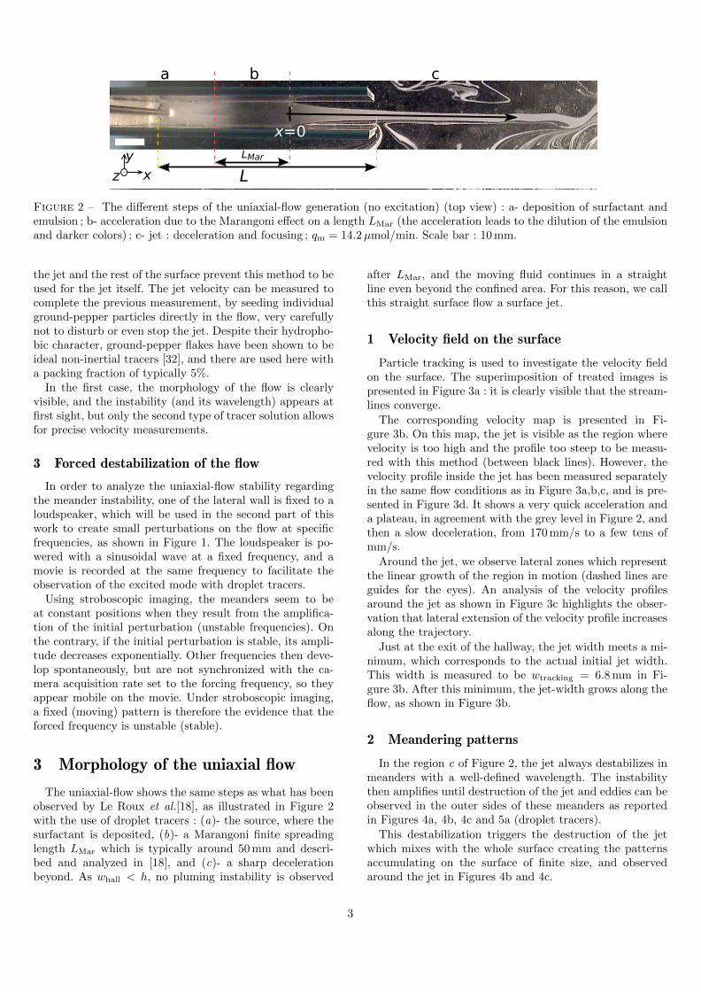
Figure 2 – The different steps of the uniaxial-flow generation (no excitation) (top view) : a- deposition of surfactant andemulsion ; b- acceleration due to the Marangoni effect on a length LMar (the acceleration leads to the dilution of the emulsionand darker colors) ; c- jet : deceleration and focusing ; qm = 14.2µmol/min. Scale bar : 10 mm.
the jet and the rest of the surface prevent this method to beused for the jet itself. The jet velocity can be measured tocomplete the previous measurement, by seeding individualground-pepper particles directly in the flow, very carefullynot to disturb or even stop the jet. Despite their hydropho-bic character, ground-pepper flakes have been shown to beideal non-inertial tracers [32], and there are used here witha packing fraction of typically 5%.
In the first case, the morphology of the flow is clearlyvisible, and the instability (and its wavelength) appears atfirst sight, but only the second type of tracer solution allowsfor precise velocity measurements.
3 Forced destabilization of the flow
In order to analyze the uniaxial-flow stability regardingthe meander instability, one of the lateral wall is fixed to aloudspeaker, which will be used in the second part of thiswork to create small perturbations on the flow at specificfrequencies, as shown in Figure 1. The loudspeaker is po-wered with a sinusoidal wave at a fixed frequency, and amovie is recorded at the same frequency to facilitate theobservation of the excited mode with droplet tracers.
Using stroboscopic imaging, the meanders seem to beat constant positions when they result from the amplifica-tion of the initial perturbation (unstable frequencies). Onthe contrary, if the initial perturbation is stable, its ampli-tude decreases exponentially. Other frequencies then deve-lop spontaneously, but are not synchronized with the ca-mera acquisition rate set to the forcing frequency, so theyappear mobile on the movie. Under stroboscopic imaging,a fixed (moving) pattern is therefore the evidence that theforced frequency is unstable (stable).
3 Morphology of the uniaxial flow
The uniaxial-flow shows the same steps as what has beenobserved by Le Roux et al.[18], as illustrated in Figure 2with the use of droplet tracers : (a)- the source, where thesurfactant is deposited, (b)- a Marangoni finite spreadinglength LMar which is typically around 50 mm and descri-bed and analyzed in [18], and (c)- a sharp decelerationbeyond. As whall < h, no pluming instability is observed
after LMar, and the moving fluid continues in a straightline even beyond the confined area. For this reason, we callthis straight surface flow a surface jet.
1 Velocity field on the surface
Particle tracking is used to investigate the velocity fieldon the surface. The superimposition of treated images ispresented in Figure 3a : it is clearly visible that the stream-lines converge.
The corresponding velocity map is presented in Fi-gure 3b. On this map, the jet is visible as the region wherevelocity is too high and the profile too steep to be measu-red with this method (between black lines). However, thevelocity profile inside the jet has been measured separatelyin the same flow conditions as in Figure 3a,b,c, and is pre-sented in Figure 3d. It shows a very quick acceleration anda plateau, in agreement with the grey level in Figure 2, andthen a slow deceleration, from 170 mm/s to a few tens ofmm/s.
Around the jet, we observe lateral zones which representthe linear growth of the region in motion (dashed lines areguides for the eyes). An analysis of the velocity profilesaround the jet as shown in Figure 3c highlights the obser-vation that lateral extension of the velocity profile increasesalong the trajectory.
Just at the exit of the hallway, the jet width meets a mi-nimum, which corresponds to the actual initial jet width.This width is measured to be wtracking = 6.8 mm in Fi-gure 3b. After this minimum, the jet-width grows along theflow, as shown in Figure 3b.
2 Meandering patterns
In the region c of Figure 2, the jet always destabilizes inmeanders with a well-defined wavelength. The instabilitythen amplifies until destruction of the jet and eddies can beobserved in the outer sides of these meanders as reportedin Figures 4a, 4b, 4c and 5a (droplet tracers).
This destabilization triggers the destruction of the jetwhich mixes with the whole surface creating the patternsaccumulating on the surface of finite size, and observedaround the jet in Figures 4b and 4c.
3
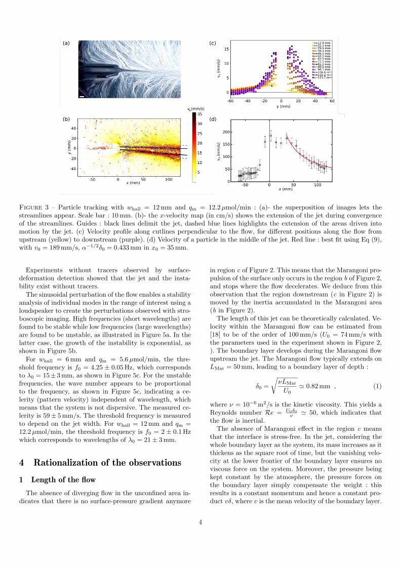
Figure 3 – Particle tracking with whall = 12 mm and qm = 12.2µmol/min : (a)- the superposition of images lets thestreamlines appear. Scale bar : 10 mm. (b)- the x-velocity map (in cm/s) shows the extension of the jet during convergenceof the streamlines. Guides : black lines delimit the jet, dashed blue lines highlights the extension of the areas driven intomotion by the jet. (c) Velocity profile along cutlines perpendicular to the flow, for different positions along the flow fromupstream (yellow) to downstream (purple). (d) Velocity of a particle in the middle of the jet. Red line : best fit using Eq (9),with v0 = 189 mm/s, α−1/2δ0 = 0.433 mm in x0 = 35 mm.
Experiments without tracers observed by surface-deformation detection showed that the jet and the insta-bility exist without tracers.
The sinusoidal perturbation of the flow enables a stabilityanalysis of individual modes in the range of interest using aloudspeaker to create the perturbations observed with stro-boscopic imaging. High frequencies (short wavelengths) arefound to be stable while low frequencies (large wavelengths)are found to be unstable, as illustrated in Figure 5a. In thelatter case, the growth of the instability is exponential, asshown in Figure 5b.
For whall = 6 mm and qm = 5.6µmol/min, the thre-shold frequency is f0 = 4.25 ± 0.05 Hz, which correspondsto λ0 = 15± 3 mm, as shown in Figure 5c. For the unstablefrequencies, the wave number appears to be proportionalto the frequency, as shown in Figure 5c, indicating a ce-lerity (pattern velocity) independent of wavelength, whichmeans that the system is not dispersive. The measured ce-lerity is 59± 5 mm/s. The threshold frequency is measuredto depend on the jet width. For whall = 12 mm and qm =12.2µmol/min, the threshold frequency is f0 = 2 ± 0.1 Hzwhich corresponds to wavelengths of λ0 = 21± 3 mm.
4 Rationalization of the observations
1 Length of the flow
The absence of diverging flow in the unconfined area in-dicates that there is no surface-pressure gradient anymore
in region c of Figure 2. This means that the Marangoni pro-pulsion of the surface only occurs in the region b of Figure 2,and stops where the flow decelerates. We deduce from thisobservation that the region downstream (c in Figure 2) ismoved by the inertia accumulated in the Marangoni area(b in Figure 2).
The length of this jet can be theoretically calculated. Ve-locity within the Marangoni flow can be estimated from[18] to be of the order of 100 mm/s (U0 = 74 mm/s withthe parameters used in the experiment shown in Figure 2,). The boundary layer develops during the Marangoni flowupstream the jet. The Marangoni flow typically extends onLMar = 50 mm, leading to a boundary layer of depth :
δ0 =
√νLMar
U0' 0.82 mm , (1)
where ν = 10−6 m2/s is the kinetic viscosity. This yields aReynolds number Re = U0δ0
ν ' 50, which indicates thatthe flow is inertial.
The absence of Marangoni effect in the region c meansthat the interface is stress-free. In the jet, considering thewhole boundary layer as the system, its mass increases as itthickens as the square root of time, but the vanishing velo-city at the lower frontier of the boundary layer ensures noviscous force on the system. Moreover, the pressure beingkept constant by the atmosphere, the pressure forces onthe boundary layer simply compensate the weight : thisresults in a constant momentum and hence a constant pro-duct vδ, where v is the mean velocity of the boundary layer.
4

Figure 4 – Different jets presenting various shapes during destabilization (not excited), always with a clear wavelength.The flow rate of surfactant deposition and the length of the hallway have been changed for the different pictures. Red dashedlines represent the middle line of the stream. (a) : qm = 14.2µmol/min and L = 100 mm. (b) : qm = 12.2µmol/min andL = 100 mm. (c) : qm = 8.1µmol/min and L = 30 mm. Scale bar : 10 mm.
0 1 2 3
Time (s)
10-1
100
101
Am
plitu
de (
mm
)
0 1 2 3 4 50.0
0.1
0.2
0.3
0.4
0.5
k (r
ad
mm
1)
f (Hz)
(mm
)
62.8
31.4
20.9
15.7
12.6
stableunstable
(a)
(c)(b)
Figure 5 – (a) The stroboscopic observation highlights theregularity of the instability at the forced frequency. Widthof hallway : 12 mm, excitation and acquisition : f = 4 Hz.Vertical dashed lines are guides for the eyes. Scale bar :10 mm. (b) Exponential growth of the amplitude for a jetof width whall = 6 mm excited at a frequency of 4 Hz. Thedotted line show the exponential growth with the growthrate of 1.344 s−1. (c) Wave number k = 2π/λ (correspon-ding wavelength on the right axis) measured for the dif-ferent excitation frequencies, width whall = 6 mm and flowrate qm = 5.6µmol/min. Dashed line represent the celerityof 59± 5 mm/s.
The shape of the velocity profile is investigated through ascaling-law analysis : considering initial conditions of velo-city v0 and boundary layer δ0 in x = x0, the momentumscales as
p ∼ v(x)δ(x) . (2)
and its conservation yields :
v(x)δ(x) ∼ v0δ0 . (3)
The vorticity oriented along y scales as :
Ω ∼ v
δ∼ p
δ2. (4)
The boundary-layer profile results from the advection-diffusion of vorticity :
v∂ Ω
∂ x= ν∆Ω , (5)
which yieldsp
δ
p
δ3d δ
dx∼ ν p
δ4, (6)
and finally :d δ
dx∼ ν
p∼ ν
v0δ0. (7)
It follows that the profile of boundary-layer depth and sur-face speed are :
δ(x) = δ0
(1 +
αν
v0δ20(x− x0)
), (8)
and
v(x) = v0
(1 +
αν
v0δ20(x− x0)
)−1
, (9)
where α is a numerical prefactor that is assumed to be closeto unity, and will be determined experimentally.
Equation (8) shows that even though the boundary layergrows with a square-root scaling in time, it follows a lineargrowth with respect to the position. Also, Equation (9) forthe initial conditions v0 = 74 mm/s and δ0 = 0.82 mm inx0 = 0 shows that velocity is divided by two on a lengthv0δ
20/ν = 50 mm (for α = 1), giving a typical length scale
for the jet in agreement with experiments, as shown inFigure 3. More precisely, using Equation (9), the best fitof the experimental data is shown in Figure 3d by thered line and show a very good agreement between ourtheoretical prediction, and the measurements. The obtai-ned values are v0 = 189 mm/s, and α−1/2δ0 = 0.433 mm
5

in x0 = 35 mm. The theoretical depth of the boundarylayer built during the Marangoni flow upstream the jet isδ0 =
√νx0/v0 = 0.430 mm, which yields the numerical pre-
factor α = 0.986, that can reasonably be considered equalto 1.
The good agreement between the experimental velocityprofile and the theory shows that the jet is indeed a surfaceflow due to the inertia accumulated in the boundary layerduring the fast Marangoni flow upstream.
2 Jet-width determination
Here we discuss the apparent contradiction between theconvergence of trajectories in Figure 3a and the widening ofthe flow in Figure 3b,c. This is common in fluid flows [33],and comes from the choice of Lagrangian or Eulerian speci-fication : from a Lagrangian point of view, the jet converges,as shown by the streamlines in Figure 3a : a physical volumeof fluid tends to go towards the center of the jet. However,from an Eulerian point of view, each moving volume trans-fers momentum to its neighbors, making the region of highvelocity extend along the path of the jet, as visible in Fi-gure 3b.
This experiment shows that the jet is actually larger thanwhat is observed with the oil-droplet tracers. Indeed, oil-droplets tracers mark only the streamlines coming from thesource (defining an apparent width wemulsion), while particletracking shows the whole extent of the high-speed area,defining the actual width of the jet : wtracking.
3 Meandering instability
Several types of instabilities have been studied in the li-terature that could correspond to what is observed in theseexperiments : the Kelvin-Helmholtz instability [34], the vis-cous thread meandering [35], or folding [36], the swirling ofcoupled threads [37], the zig-zag instability of vertices [38],Von-Karman streets [39], or Rayleigh’s development of theKelvin-Helmholtz instability for vorticity bands [40].
Each black/white frontier in Figure 4 shows the charac-teristic features of a Kelvin Helmholtz instability [34, 41].The anti-symmetry of the patterns facing each other sug-gests that the two instabilities are coupled. These two ob-servations and the measurements detailed previously indi-cate that the present phenomenon is one of the instabilitiesdescribed by Rayleigh [40], and more precisely the Kelvin-Helmholtz destabilization of two coupled and adjacent vor-ticity bands, as sketched in Figure 6.
Let’s summarize the hypothesis and conclusions of Ray-leigh. Considering two adjacent bands of vorticity of widthb > 0 of opposite signs, corresponding to a triangular ve-locity profile illustrated in Figure 6, the destabilization ofthe two adjacent vorticity bands is investigated. Novelty ofRayleigh’s study is the non-zero width of the vorticity band(a linear velocity profile instead of a step profile), and thepossible coupling between two bands. This model, initiallydeveloped to study a 3D jet, actually describes very preci-sely the present experiments : it corresponds to both our
VX
Z2bz xy
Figure 6 – Velocity profile (black) and vorticity profile(red) of the jet studied theoretically by Rayleigh[40].
initial configuration (two vorticity bands) and its destabili-zation (meandering with long wavelengths).
The result of Rayleigh’s calculations is that the two sidesof the jet are coupled, and that destabilization always oc-curs with anti-symmetric deformations, leading to mean-ders growing exponentially, while all the other deforma-tion modes are stable. Moreover, only short wavelengthsλ < λ0 = πb are expected to be stable, and the fastest des-tabilization occurs for λM = 8πb/5 ' 5b, but the growthrate is close to its maximum on a large range of frequen-cies. Finally, according to the classical Kelvin-Helmholtzanalysis, the instability is expected to move with a celeritywhich is half of the maximum velocity of the jet. This is allconsistent with our observations.
Kelvin-Helmholtz instabilities perpendicular to the inter-face are hindered by interfacial tension and density mis-match between air and water until a threshold speed [42]of 1.5 m/s, which is never reached in these experiments.
For the free jet as pictured in Figure 2 and 4, as noneof the modes is forced, the observed ones are the fastest,or a superposition of all the wavelengths around λM. Wa-velengths observed on Figure 4a (λM = 12.8 ± 3 mm),Figure 4b (λM = 16.5 ± 3 mm) and Figure 4c (λM =8.1± 3 mm) yield values for the jet width of 5.1± 0.6 mm,6.6 ± 0.6 mm and 3.2 ± 0.6 mm respectively. However, dueto the intrinsic low wavelength selectivity of the instability,the wavelength are not as well defined as for the excited jet(see Figure 5a).
For the forced destabilization, the measured celerity ofthe instability for whall = 6 mm, extracted from Figure 5b,is independent of the frequency , in agreement with theKelvin-Helmoltz theory, and equal to c = 59 ± 5 mm/s.This value must be compared with the velocity profile fromparticle tracking shown in Figure 3b and Figure 3d. Par-ticle tracking close to the jet shows velocities of the orderof 3 cm/s, and the velocity inside the jet decreases from150 mm/s to 50 mm/s along the flow. The celerity of thepatterns corresponds to a fraction of the jet velocity, slightlydifferent from the Kelvin-Helmholtz prediction, which iscalculated for a step-profile. The threshold frequencies λ0measured in the previous section correspond to jet widthsof wRayleigh = 4.8 ± 0.6 mm when whall = 6 mm, andwRayleigh = 2b = 6.7 ± 0.6 mm when whall = 12 mm.This second value can be compared with what has beenmeasured with particle tracking and shown in Figure 3b(wtracking = 6.8 ± 0.25 mm). Particle tracking and instabi-
6

lity analysis show a very good agreement on the jet width.
5 Summary and conclusion
Spreading of soluble surfactants occurs over a finite dis-tance on the surface, but the effects of the Marangoni floware observed on a much larger length scale due to the inertiaprovided to the fluid in the Marangoni flow. Lateral confi-nement of the flow can change the extent of these inertialsecondary flows. Indeed, if the flow is narrow enough, aswe investigated here, a huge increase of the extent of thesesecondary flows is observed, and the flow forms an inertialsurface jet.
Flows are also induced through all the surface thatconverge towards the origin of the jet. Thanks to tracersinside the jet and on the whole surface, a full picture of theflow on the surface is exhibited, by combining two types oftracers providing complementary information. The velocityprofile of the jet is predicted analytically and successfullycompared with the experimental measurements.
Finally, the straight jet eventually destabilizes intomeanders. Qualitatively, the observed features are : anti-symmetric patterns (no varicose patterns), a large wave-length compared to the jet width, and eddies in the ou-ter sides of the meanders. This instability is characterizedquantitatively by forcing specific frequencies : the domainof instability is identified, and wavelength measurementsshow that the celerity of the patterns is independent of thefrequency. These features are the signature of a situationdescribed by Rayleigh that was never observed for surfaceflows yet. Quantitative comparison between the theory andthe experimental observations yields a very good agreementin terms of threshold frequencies.
We have characterized and understood the 2D flows crea-ted by this configuration of soluble-surfactant directionalspreading under lateral confinement. This is a first step tounderstand the role of inertial effects in the Marangoni flowswith and without confinement. Not only this work paves theway towards a better control of the flows involved in foamand coating processes, but also it brings a new light in thestudy of Marangoni propulsion for natural or artificial sur-face micro-swimmers.
Acknowledgements
The authors thanks Aberrazzaq Moufidi for his help incapturing the surface deformation, and Isabelle Cantat andFrancois Charru for the helpful discussions.
References
[1] Chang Won Park. Effects of insoluble surfactants ondip coating. Journal of Colloid And Interface Science,146(2) :382–394, 1991.
[2] Laurie Saulnier, Frederic Restagno, Jerome Delacotte,Dominique Langevin, and Emmanuelle Rio. What is
the mechanism of soap film entrainment ? Langmuir,27(22) :13406–13409, 2011.
[3] Jacopo Seiwert, Benjamin Dollet, and Isabelle Cantat.Theoretical study of the generation of soap films : Roleof interfacial visco-elasticity. Journal of Fluid Mecha-nics, 739 :124–142, 2014.
[4] Emmanuelle Rio and Francois Boulogne. Withdrawinga solid from a bath : How much liquid is coated ? Ad-vances in Colloid and Interface Science, 247 :100–114,2017.
[5] V G Levich and V S Krylov. Surface-tension-drivenphenomena. Annual Review of Fluid Mechanics,1(1) :293–316, 1969.
[6] PR Garrett. Defoaming : theory and industrial appli-cations, volume 45. CRC Press, 1992.
[7] Nikolai D. Denkov. Mechanisms of foam destructionby oil-based antifoams. Langmuir, 20(22) :9463–9505,2004.
[8] D. Langevin. Rheology of adsorbed surfactant mono-layers at fluid surfaces. Annual Review of Fluid Me-chanics, 46(1) :47–65, 2014.
[9] V. Miralles, B. Selva, I. Cantat, and M. C. Jullien.Foam drainage control using thermocapillary stress ina two-dimensional microchamber. Physical Review Let-ters, 112(23) :1–5, 2014.
[10] Veronique Pimienta, Michele Brost, Nina Kovalchuk,Stefan Bresch, and Oliver Steinbock. Complex shapesand dynamics of dissolving drops of dichlorome-thane. Angewandte Chemie - International Edition,50(45) :10728–10731, 2011.
[11] Alvaro Marin, Robert Liepelt, Massimiliano Rossi, andChristian J. Kahler. Surfactant-driven flow transitionsin evaporating droplets. Soft Matter, 12(5) :1593–1600,2016.
[12] F. Wodlei, J. Sebilleau, J. Magnaudet, and V. Pi-mienta. Marangoni-driven flower-like patterning of anevaporating drop spreading on a liquid substrate. Na-ture Communications, 9(1) :820, 2018.
[13] Ziane Izri, Marjolein N. van der Linden, SebastienMichelin, and Olivier Dauchot. Self-Propulsion ofPure Water Droplets by Spontaneous Marangoni-Stress-Driven Motion. Physical Review Letters,113(24) :248302, dec 2014.
[14] Yasuhiro Ikezoe, Gosuke Washino, Takashi Uemura,Susumu Kitagawa, and Hiroshi Matsui. Autonomousmotors of a metal-organic framework powered by reor-ganization of self-assembled peptides at interfaces. Na-ture Materials, 11(12) :1081–1085, 2012.
[15] John W.M. Bush and David L. Hu. WALKING ONWATER : Biolocomotion at the Interface. Annual Re-view of Fluid Mechanics, 38(1) :339–369, 2006.
[16] Eric Lauga and Anthony M.J. Davis. Viscous Maran-goni propulsion. Journal of Fluid Mechanics, 705 :120–133, 2012.
7

[17] D. G. Suciu, Octavian Smigelschi, and Eli Ruckenstein.Some experiments on the Marangoni effect. AIChEJournal, 13(6) :1120–1124, 1967.
[18] Sebastien Le Roux, Matthieu Roche, Isabelle Cantat,and Arnaud Saint-Jalmes. Soluble surfactant sprea-ding : How the amphiphilicity sets the Marangoni hy-drodynamics. Physical Review E, 93(1) :1–13, 2016.
[19] Shreyas Mandre. Axisymmetric spreading of surfac-tant from a point source. Journal of Fluid Mechanics,832 :777–792, dec 2017.
[20] Thomas Bickel. Spreading dynamics of reactive sur-factants driven by Marangoni convection. Soft Matter,15(18) :3644–3648, 2019.
[21] Ye Tian, xiaoying Gao, Wei Hong, Miao Du, PengjuPan, Jing Zhi Sun, Zi Liang Wu, and Qiang Zheng.Kinetic Insights into Marangoni-Effect-Assisted Pre-paration of Ultrathin Hydrogel Films. Langmuir,34 :acs.langmuir.8b02626, 2018.
[22] Amar S. Basu and Yogesh B. Gianchandani. Virtualmicrofluidic traps, filters, channels and pumps usingMarangoni flows. Journal of Micromechanics and Mi-croengineering, 18(11) :115031, nov 2008.
[23] H. Kellay, X. L. Wu, and W. I. Goldburg. Experimentswith turbulent soap films. Physical Review Letters,74(20) :3975–3978, 1995.
[24] Michael Rivera, Peter Vorobieff, and Robert E. Ecke.Turbulence in flowing soap films : Velocity, vorti-city, and thickness fields. Physical Review Letters,81(7) :1417–1420, 1998.
[25] C. H. Bruneau and H. Kellay. Experiments and directnumerical simulations of two-dimensional turbulence.Physical Review E - Statistical, Nonlinear, and SoftMatter Physics, 71(4) :1–5, 2005.
[26] Matthieu Roche, Zhenzhen Li, Ian M. Griffiths, Sebas-tien Le Roux, Isabelle Cantat, Arnaud Saint-Jalmes,and Howard A. Stone. Marangoni flow of soluble am-phiphiles. Physical Review Letters, 112(20) :1–5, 2014.
[27] M. M. Bandi, V. S. Akella, D. K. Singh, R. S. Singh,and S. Mandre. Hydrodynamic Signatures of Statio-nary Marangoni-Driven Surfactant Transport. Physi-cal Review Letters, 119(26) :1–5, 2017.
[28] Anastasia Shmyrova and Andrey Shmyrov. Instabilityof a homogeneous flow from a lumped source in thepresence of special boundary conditions on a free sur-face. EPJ Web of Conferences, 213 :02074, jun 2019.
[29] I. K. Bratukhin and L. N. Maurin. Convection inf afluid-filling half space. PMM, 31(3) :577–580, 1967.
[30] Iu K. Bratukhin and L. N. Maurin. Stability ofthermocapillary convection in a fluid filling a half-space. Journal of Applied Mathematics and Mechanics,46(1) :129–131, 1982.
[31] Anne D. Dussaud and Sandra M. Troian. Dynamicsof spontaneous spreading with evaporation on a deepfluid layer. Physics of Fluids, 10(1) :23–38, 1998.
[32] M. M. Bandi, T. Tallinen, and L. Mahadevan. Shock-driven jamming and periodic fracture of particulaterafts. Epl, 96(3), 2011.
[33] K. R. Reddy and R. I. Tanner. Finite element solutionof viscous jet flows with surface tension. Computersand Fluids, 6(2) :83–91, 1978.
[34] P. Gondret and M. Rabaud. Shear instability of two-fluid parallel flow in a Hele-Shaw cell. Physics ofFluids, 9(11) :3267–3274, 1997.
[35] Stephen W. Morris, Jonathan H.P. Dawes, Neil M.Ribe, and John R. Lister. Meandering instability ofa viscous thread. Physical Review E - Statistical, Non-linear, and Soft Matter Physics, 77(6) :1–11, 2008.
[36] Thomas Cubaud and Thomas G. Mason. Folding ofviscous threads in diverging microchannels. PhysicalReview Letters, 96(11) :1–4, 2006.
[37] Thomas Cubaud and Thomas G. Mason. Swirling ofviscous fluid threads in microchannels. Physical ReviewLetters, 98(26) :2–5, 2007.
[38] Paul Billant and Jean Marc Chomaz. Experimentalevidence for a new instability of a vertical columnarvortex pair in a strongly stratified fluid. Journal ofFluid Mechanics, 418 :167–188, 2000.
[39] E. Detemple-Laake and H. Eckelmann. Phenomeno-logy of Karman vortex streets in oscillatory flow. Ex-periments in Fluids, 7(4) :217–227, 1989.
[40] Lord Rayleigh. On the Stability, or Instability, of cer-tain Fluid Motions. Proceedings of the London Mathe-matical Society, s1-11(1) :57–72, nov 1879.
[41] S. A. Thorpe. A method of producing a shear flow in astratified fluid. Journal of Fluid Mechanics, 32(4) :693–704, 1968.
[42] E Guyon, J-P Hulin, L Petit, CD Mitescu, and DF Jan-kowski. Physical Hydrodynamics. Applied MechanicsReviews, 55(5) :B96–B97, sep 2002.
8