stability of angle-section members
TRANSCRIPT

STABILITY OF ANGLE—SECTION MEMBERS
by
R.T.G. Green, B.E. (Hons.)
submitted in partial fulfilment of the requirements
for the degree of
Master of Engineering Science,
0 UNIVERSITY OF TASMANIA
HOBART.
— AUGUST, 1967 —

SUMMARY
A simple treatment of the elastic stability of angle-piectio#
members, both columns and beams, has been developed, based on the
measured deformations of typical members loaded in the laboratory°
Detailed mathematical models describing the torsiOnal,or local
buckling modes of the members are presented° Other buckling modes
have been considered and the interaction of the various modes has P
been discussed. Angle.-section columns, eccentrically loaded
columns, cantilevers, centrally-loaded simply-supported beams, and
laterally loaded columns, have been studied in particular.
I hereby declare that, except as stated herein, this
thesis contains no material which has been accepted
for the award of any other degree or diploma in any
University, and that, to the best of my knowledge or
belief the thesis contains no copy of paraphrase of
material previously published or written by another
person, except where due reference is made in the
text of this thesis.

- INDEX -
INTRODUCTION 1
GEOMETRY AS A WORKING TOOL
4
Ligtenberg Moire Method
Crossed Diffraction Grating Moire Method
BUCKLING 11
Columns
Plate Structures
Energy
Stability of Systems Governed by Differential Equations
Stability of Systems Governed by Simultaneous Linear
Equations
Finite Difference Methods
A System of n Degrees of Freedom
TORSION 24
BUCKLING OF COLUMNS
Load Applied Through a Base Plate 29
First Mathematical Model - Small Elastic
Deflections
Second Mathematical Model - Small Elastic
Deflections
Initial Shape
Third Mathematical Model - Large Elastic
Deflections
Eccentric Loading
Applied Torque
Columns with Bolted End Conditions 4 5
First Mathematical Model
Second Mathematical Model
Stress Distribution Around a Bolt
Torsional-Flexural Buckling 58

- INDEX-
STABILITY OF ANGLE-SECTION BEAMS
Stability of Angle-Section Cantilevers 6 5
Small Elastic Deflection Mathematical Model
Large Elastic Deflection Mathematical Model
Fully Plastic Mathematical Model
Lateral Buckling of Cantilever 74
Simply Supported Beams 76
Central Load
Uniform Bending Moment
Combined Axial and Lateral Buckling 79
CONCLUSIONS
Appendix A
Appendix B
Notation
ACKNOWLEDGEMENTS
This work was carried out in the Civil Engineering Department
of the University of Tasmania. The author wishes to thank the
members of the staff of the University. In particular the author
wishes to thank Professor A.R. Oliver, Professor of Civil Engineering,
and Dr. M.S. Gregory, my supervisor of research, for their help and
encouragement.

INTRODUCTION
Angle-section members, under various loading conditions, have
been found to be unstable. In this thesis the conditions under which
the instability occurs are presented and mathematical models are form-
ulated to describe the geometry of the deformed member and to calculate
the load capacity of the member. Equal-leg angle-section members were
tested as columns, eccentrically loaded columns, cantilevers, centrally
loaded beams, and laterally loaded columns. The mathematical models
which are developed herein describe the torsional and local buckling of
the members. However, where applicable, other types of instability
have been investigated; also some types of interaction which can occur
between the possible modes of buckling have been considered.
Only relatively recently, the torsional and local properties
of structural members have become important. With the introduction
of slender high-strength steel members, and materials such as aluminium
and its alloys with low moduli of elasticity, the problem has been
accentuated. Even today most design codes are based upon practices
developed for mild steel members. In this century, considerable work
has been carried out on the instability properties of columns. Two
organisations which are particularly interested in the problem are the
Column Research Council of America1and the Aluminium Research Develop-
2 ment Association of Britain. Both organisations have published results
or codes which could be used by practising engineers. The German code
is one of the most progressive codes.
In this thesis the problem of the buckling of angle-section mem-
bers has been investigated using a new approach. Large field methods
of measuring geometrical shapes have been used to obtain the deformed
shape of the member. The basic geometry is then described analytically
and the analytic function is used as a basis for the mathematical model.
The forces required to sustain the measured deformation are calculated
and a differential equation is obtained by considering the statical
equilibrium of the whole member. The analytic function describing the
geometry can be specified to any order of approximation and consequently
Ref. 1 Column Research Council Guide to Design Criteria for Metal Com-pression Members, John Wiley & Sons, Inc.
Ref. 2 Series of Aluminium Research Development Association Reports.

- 2-
a number of successively more satisfactory mathematical models can be
derived to describe the physical behaviour.
For most cross-sections the member can buckle either by the whole
cross-section rotating, in an undeformed state, or by part of the cross-
section defoIrming. The first type of instability is referred to as a
torsional instability and the second as a local instability. For an
equal-leg angle-section member, with both leg's loaded identically,
torsional buckling and local buckling are the same phenomena, and the
two terms are interchanged freely in all the literature. Under this
loading each leg acts as a simply supported plate, and there is no mom-
ent acting around the corner of the cross-section. The buckling of an
angle member has been treated by these various methods, each of which
will be considered.
The models tested were of such dimensions that the torsional mode
was prominent, To emphasize torsional buckling behaviour the members
tested had thinner walls, relative to width of leg, than are common in
practice, but it has been indicated how the results obtained can be
amended to give an understanding of the behaviour of more practical
sections.
This thesis does not set out to present a large quantity of
results and to derive empirical formulae or relationships. Rather, it
relies on the similarity of the geometry of the deformation of members
of different proportions and sizes. The mathematical models developed
are based upon the deformed geometry of a number of members tested in the
laboratory, and the results derived are compared with those obtained from
a few physical models. In the future, large-scale testing programmes
for more practical members might be contemplated; it is thought that the
necessary basic ideas are established in this thesis,
This thesis is divided into four parts. The first part is
devoted to forming a foundation upon which the author's work is built.
Although no new ideas are presented therein, the understanding of the
ideas is basic to the remainder of the thesis,
The second section deals with the stability of a column which is
axially loaded with a uniform stress distribution. Results presented

- 3 -
in this part have been derived in detail, because many of the ideas are
used in the following sections. The work on a column under a pure axial
load was presented by the author as a partial requirement for an honours
bachelor's degree. In this thesis, the topic has been expanded by
including the effect of non-uniform stress distribution produced by load-
ing the member through a bolt. A detailed comparison with other math-
ematical models is also presented.
The third section deals with the instability of angle-section
beams. This section leans heavily on the preceding section as it uses
basically the same logic, although the mathematical models developed are
more complicated. To the author's knowledge, there exist no other math-
ematical models which describe this problem, although beam-columns have
been treated empirically.
The fourth section, a detailed comparison between the results
obtained in this thesis and those obtained by other mathematical models
is given. Present design codes are considered, and possible amendments
are suggested in the light of the results of the work described in the
thesis, and the fundamental understanding which it has encouraged or made
possible.
This thesis establishes a new, simple mathematical model for the
elastic behaviour of a column, and original mathematical models for the
torsional buckling of a cantilever and a centrally loaded simply supported
beam. Although the author has presented a mathematical model for a
laterally loaded column, this topic needs further investigation. The
thesis also considers the mathematical models describing the torsional-
flexural buckling of a column developed by other workers, and the rel-
evance of the lateral buckling model of beams developed by Tunoshenko.

GEOMETRY AS A WORKING TOOL
In the history of engineering structural science, the basic under-
standing of the geometry of the deformations of a loaded member has led to
the necessary valuable simplifications on which all analysis is based, and
has thus played an important part in the advancement of the science.
Geometry has the advantage that it can be easily measured. From the
earliest problem, that of a loaded cantilever, the geometry has been the
basis for the mathematical description. The theory of bending is based
upon the geometrical assumption that plane sections remain plane. However,
the parameters of the geometry must be evaluated by considering the stat-
ical equilibrium of the member. The early development of the theory of
bending was slow, as the experimenters failed to combine the geometry and
the equations of equilibrium. In fact, this lack of completeness in the
model led early engineers to assume that the neutral axis of a beam in bend-
ing was at the lower edge.
Later, prominent men, such as Timoshenko, have made advances
because they have been able to base their mathematical descriptions upon
geometry. One example, which was developed during this century, is the
plastic analysis of members. Plastic analysis has become important because
of the simplicity of its application, which in turn depends upon a simple
deformation pattern. A framed structure in a fully plastic state is
described by a rigid-plastic load-deformation relationship, in which all
deformations occur within local regions known as plastic hinges. Lately,
more sophisticated descriptions of elastic-plastic bending have been
produced in which other deformations have been included.
The author will consider the torsional buckling of angle-section
members by measuring the geometry of the member in its deformed or buckled
state. The geometrical approach has been made possible by the develop-
ment of optical methods of measuring geometry over large fields of view.
Two such methods are the photo-elastic method, which measures stress in
the plane of the model, and the moire fringe techniques, which measure
deflections both in and normal to the plane of the model. For the work
described here the moire fringe methods have been used, as they measure
geometry directly.

white grey fringe
fringe
MOIRE FRINGES FIGURE 1.
AB and A'Bi are the initial and the final slopes of the plate at 0. ROI and Q0I are two rays. I is the image of both Q and R.
LIGTENBERG APPARATUS FIGURE 2.

5
Moire Fringes
When two sets of parallel lines are interfered, a moire fringe
pattern is formed as shown in fig. 1. Where two lines intersect, a
"white" fringe is formed, while a grey fringe occurs when a white and a
black line intersect. In interference terms, a "white" fringe occurs
when the lines are in phase, that is displaced by an integral number of
line spaces. The "grey" fringes are formed when the lines are out of
phase.
Two of the available moire fringe methods have been used by the
author in his experimental work. One method, the Ligtenberg method,
measures changes in slope of a surface. The other method measures
deflections in the plane of the surface. In this section of the thesis
the author will only outline the experimental methods used. For complete
details, such as the production of gratings, and the preparation of the
models, reference may be made to Ligtenberg's1 paper and two papers by
2 Middleton, Jenkins and Stephenson;'
3 the latter workers are engaged in the
development of the techniques used at the University ofTasmania. The
basic ideas involved in using the two methods are described in the follow-
ing sections.
* * * *
The Ligtenberg Method1
The Ligtenberg method produces moire fringes which are contours
of equal change in slope of a surface. The surface to be examined is
made reflective by gluing a sheet of Melanex, a commercially available
sheet of plastic coated with aluminium, to the surface. Kodaflat matte
solution, a pressure-sensitive glue is used. A set of photographically
reproduced lines is mounted on a part of a cylindrical surface and a
camera is arranged so that the lens is at the centre of the screen. The
lines are reflected from the model's surface and an image is produced on
the camera film. The model is loaded and the second exposureis taken.
Ref. 1 Ligtenberg: "The Moire Method as a new experimental method for the determination of moments in small slab models". Vol. XII, No, 2, Proc, Soc. Experimental Stress Analysis.
Ref. 2 E. Middleton and C. Jenkins: 'Moire methods for Strain Analysis for Student Use", Bulletin of Mech. Eng, Education, Issue 3, Vol, 5, 1966.
Ref. 3 E. Middleton and L.P. Stephenton: "A reflex Spectrographic Tech-nique for in-plane Strain Analysis". In printers hands. SESA Paper No. 1250.

Ligtenberg moire apparatus for measuring slope.
FIG. 3
Crossed diffraction grating method of measuring displacements in the plane of the model.
FIG. 4

-6
The double exposure produces moire fringes which are lines of constant
slope. The general arrangement of the apparatus is as shown in figs. 2
and 3.
An approximate relationship between the change of slope at each
fringe can be derived by considering the model point which lies on the
screen. The following notation will be used; d is the line spacing of
the grid, a is the radius of curvature of the screen, vf is the change
in slope of the model and n is an integer. In fig. 3, Q0I and ROI
are the ray traces for the unloaded and loaded cases respectively. The
distance QR is given approximately by 2ayi . For a "grey" fringe to
form at I QR must be equal to 2(n + i)d . Thus the slope change is
given by
yr)= (2n + i)d/2a (1)
In the following experimental work this formula has been used for all
points on the model surface. The errors involved in using this formula,
when applied to off-centre points or when the model is not at the centre
of curvature of the grid, have been indicated by Ligtenberg in his art-
icle. The slope measured is the slope in the direction normal to the
grid lines. Two photographs, with the grid lines perpendicular must be
taken to fully describe the geometry of the surface in terms of its slope
in two directions at right angles to one another.
Crossed Diffraction Grating Methods
A moire pattern is produced when two diffraction gratngs are
superimposed. Fringes are due to mis-matching of gratings or relative
rotation of the two gratings. If one of the gratings is moved relative
to the other, the pattern changes. A secondary moire fringe pattern can
be obtained by superimposing the two primary patterns. The secondary
fringes represent lines of constant displacement and are independent of
the initial primary pattern.
A grating is glued to the surface of the model and a reference
grating is fixed to the model, so that the relative movement between the
two gratings is restrained kinematically1
Usually three connections are
Ref. 1 E. Middleton and L. P. Stephenson: "A reflex Spectrographic Tech-nique for in-plane Strain Analysis". In printers hands. SESA Paper No. 1250.

used; a point at which there is no relative movement, a line where there
is movement in one direction only and a plane which allows complete free-
dom of movement and is used to maintain a constant air gap. With the
three point system the reference grating is mounted kinematically, and
the loading of the model does not load the reference grating.
Two photographs are taken of the moire fringe pattern, one of
the loaded model and another of the unloaded model. The secondary patt-
ern obtained from the two primary patterns represents lines of constant
displacement normal to the grating lines. The optical system required
to take the photographs is shown in fig. 4. The system can be broken
down into four sections, a collimator, the model, a condenser system, and
a camera,
The models used for the transmission method are made of perspex.
Gratings of one hundred, one thousand, and three thousand lines per inch
are produced at the University of Tasmania.
The moire fringes make it possible to measure the deformations
of members under load, and hence to describe the deformations analytically.
The analytic functions, in conjunction with stress-strain relationships,
can be used to consider the statics of the problem, either to determine
the loads applied or to enable a statical balance on any section or
portion of a member to be carried out. It will be appreciated that the
geometry is only approximated by the analytic functions and the degree of
approximation is important. The complexity of the mathematics must be
balanced by consideration of the accuracy with which the mathematical
description is required to agree with the physical model.
At this point it will be of benefit to introduce several terms to be used
throughout this thesis. "Functional form" is a term used to indicate any
one aspect of the geometry which is common to all problems of a certain
type. For example, "plane sections remain plane" is the functional form
for bending, and "radii remain straight" is the functional form for the
torsion of a solid circular bar. The functional form does not necessar-
ily describe the shape of the member fully. The "mode" of a buckled

8
member or structure is the critical or buckled shape (or "eigen" shape)
of the perfect member or structure. For a given structure there is
usually more than one mode.
A "mathematical model" refers to the mathematical description
which can be built up once some basic assumptions have been made. It is
important to realize there is more than one possible mathematical model
suitable for describing a physical model. In the previous example of
elastic bending, the basic assumptions are that plane sections remain
plans and that the stress-strain relationship is linear. From these
basic assumptions follow the relationships that the moment M is equal
to EIK 9 and that the stress 6 at a point equals My/El 9 where E
is Young's modulus, I is the moment of inertia about an axis through
the centroid, K is the curvature of the line of centroids, and y is
the distance from the centroidal axis. The next result, for example, is
that the shear stresses and strains are parabolically distributed in a
rectangular beam. The previous statements form one mathematical model
of elastic bending. However, it should be noted that the model has a
contradiction. It has been assumed that plane sections remain plane,
but, as a result, the shear stresses and hence the shear strains are para-
bolically distributed. This result leads to another mathematical model
in which plane sections do not remain plane. For most engineering
purposes the first mathematical model describes the physical model suff-
iciently well.
In some cases more than one mathematical model arises due to a
mathematical approximation. Consider the beam again. If one derives
the curvature distribution along the beam and uses the differential
expression for curvature,
K = b2w/ x2/(1 +
the shape of the beam can be calculated. In most cases the approximate
expression for the curvature K = b 2w/x 2 is sufficiently accurate.
Any mathematical approximation should be included in the basic assumptions
and also the limits of its application, because if the model is extended
to apply for large deflections the approximations may not apply.
In a mathematical model one tries to satisfy three conditions;
compatible geometry, the equations of statical equilibrium and the boundary

small width - thickness ratio
loading q
normal deflection w
FIGURE 5
large width - thickness ratio
THE SHAPE OF A SLAB BENT BY A UNIFORM MOMENT
FIGURE 6

- 9 -
conditions, all to a certain level of approximation. As no mathematical
model fully describes the physical model, a compromise must be reached.
in the approach taken it is relatively simple to describe a system of
compatible geometrical deformations which satisfy the boundary conditions.
However, usually only some of equations of statics are satisfied. The
potential energy method is a means of obtaining an approximate solution
in which all the equations of statics are satisfied on an average. In
fact, if the correct geometry is fed into the enetgy equation it reduces
to the equations of statics.
In establishing a mathematical model it is advisable to start
with the simplest functional form possible. Using large field measure-
ments the salient functional form is usually obtained easily, and the
order of magnitude of any secondary component can be determined. In the
previous paragraph, it has been stated that the functional form must sat-
isfy the boundary conditions. For certain problems some of the boundary
conditions have little effect on the strength of the member. The contours
of measured deformations, obtained by the moire methods, aid the invest-
igator in appreciating the important boundary conditions. Consider two
beams one with a width-thickness ratio of approximately two and another
with a large width-thickness ratio. Both beams have a curvature K x in
the direction of the applied moment. But the orthogonal curvature is
equal to -1)Kx for the first beam and zero for the second, where .1) is
Poisson's ratio (see Fig. 5)0 Obviously the second beam does not satisfy
the boundary conditions of zero moment and shear stress along the edge of
the beam. In fact, it does, because the curvature changes from zero to
x in a local region near the edge. If the curvature is assumed to
change in a certain manner the consequences of neglecting the local edge
effect can be calculated. The assumption of zero curvature across a long
flat strip leads to a simpler mathematical model. As an example, consider
a strip as a long beam, length L simply supported at each end and
carrying a load
ll'x q = q sin — L
see fig. 6 9 the differential equation for the normal deflection w of a
plate carrying a lateral load q is
, 11-w/ x4 + 2 t vv/ .62x y tw/ y4 cilD (2)

-10-
If we take w = aW(X) 9 where W(x) is a function at x only, the
differential equation simplifies to
Trx 4W/ex4 = qo/D sin --- L
and the shape is
w = qsL/Tr) 4y sin Ti!,1 9
when the boundary conditions are satisfied. Alternatively, if we use
w = W(y) sin
then the differential equation becomes
W(Tr/L) 4 - (TrA) 2 sin1rx/L 2)2w/ by2 + sinlirx/L
= q0 sinlix/L 0
This equation could be solved and the boundary conditions, zero moment
and shear stress applied. However, the mathematics are much more comp-
licated.
In buckling problems the end conditions have an important effect
on the load capacity of the model. In developing a mathematical model
for the buckling of a column, most experimenters aim either for fully
built in end conditions or for a simply supported condition. In the
experimental work associated with this thesis, no particular effort was
made to obtain a certain type of end condition. The Ligtenberg apparatus
was used to determine the end conditions. However, the mathematical
models established have been adopted to apply to members with simply supp-
orted ends, and have been presented for this case.
In this section it is hoped that the benefits of measuring the
geometry of deformations of a loaded member have been indicated: Firstly
in establishing the problem, that is in determining the boundary conditions
and indirectly the loads applied; secondly in appreciating the salient
features of the functional form. Geometry is a readily measurable prop-
erty which forms a foundation stone from which can be built, in a logical
manner, a mathematical model.
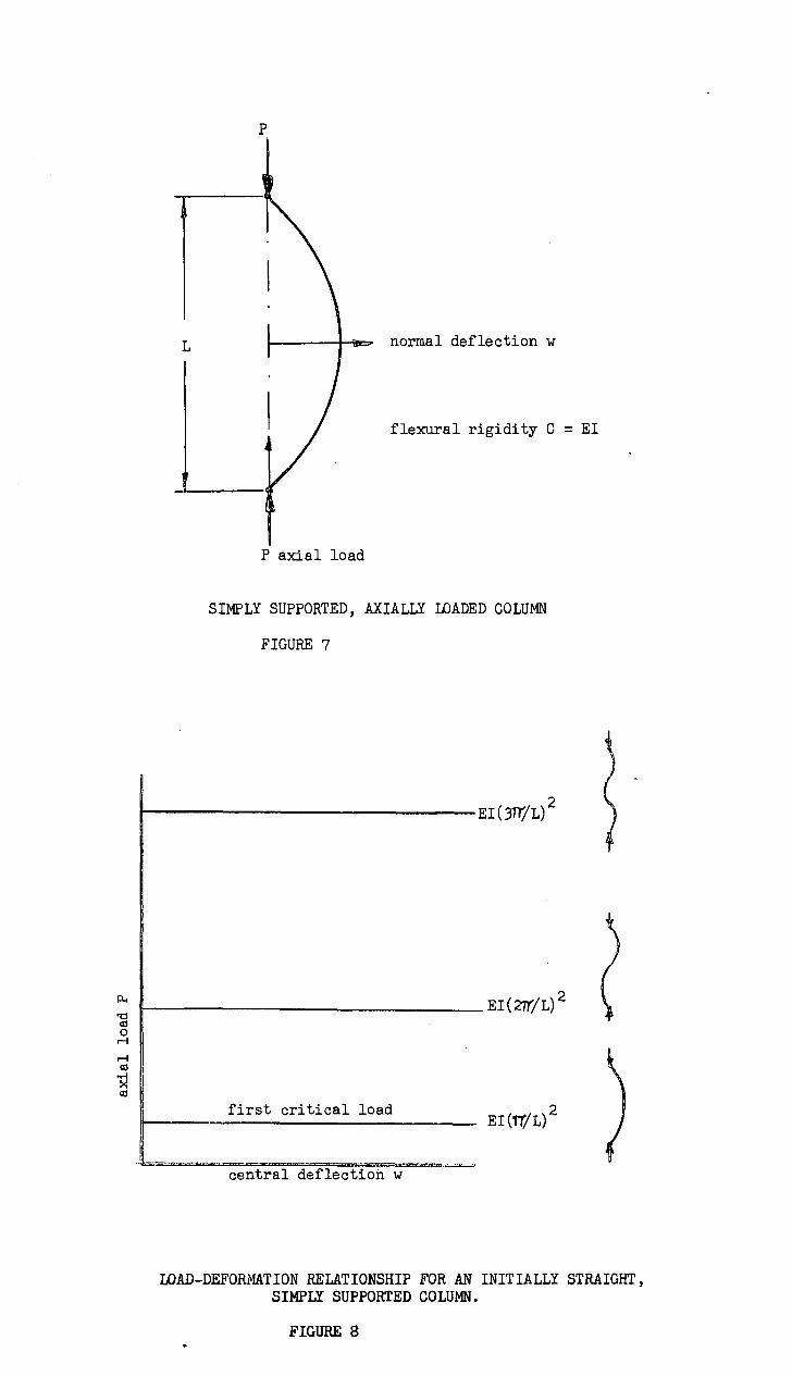
EI(3n7L)2
EI(27T/L) 2
EI(1tL) 2
first critical load
normal deflection w
flexural rigidity C = El
P axial load
SIMPLY SUPPORTED, AXIALLY LOADED COLUMN
FIGURE 7
central deflection w
LOAD-DEFORMATION RELATIONSHIP FOR AN INITIALLY STRAIGHT, SIMPLY SUPPORTED COLUMN.
FIGURES
axia
l lo
ad P

BUCKLING
A practical structure can be said to be unstable if it exper-
iences large deformations in the neighbourhood of a given load. The given
load is called the critical load. One type of instability is plastic
collapse due to the non-linearity of the load-deformation relationship of
the material. Other structures are unstable in the elastic range.
Generally the term "instability" applies only to elastic structures. It
is important to realize that the stability of the structure depends not
only on the structure but also on the loading method.
This chapter is presented as a historical review of the
of instability. However, the progress in understanding the behaviour of
a single column is considered first, as most of the ideas associated with
the general topic of buckling were established by considering a simply
supported column. Next, the buckling of plates will be considered.
Chronologically the development of the theory of the buckling of plates
lagged slightly behind that of a column. The final part of this chapter
will be devoted to ideas which apply generally to all structural and
dynamic instability problems. Both types of problems have similar diff-
erential equations.
Columns
The mathematician, Euler, first introduced a mathematical model
for the instability of an axially loaded simply supported column in the
year 1744 9 see Fig. 7. Basing his model on a linear moment-curvature
relationship and the approximate curvature expression
K = 2w/),_2 A. 9
he obtained the equation of equilibrium for the column in terms of the
normal deflection w 9
Moment = Pw C e 2w/ x2
The solution of the differential equation is trivial unless the load
has the value
crit
in which case the deflection is indeterminate. The constant C is
the flexural rigidity El 9 where E is Youngs Modulus and I is the
smallest moment of inertia. Lagrange (1770) enlarged upon Eulerls work
(3)
(4)

axial load P
central deflection
axial lo
ad p
tangential angle o< end angle S ordinate measured along the member
FIGURE 9
tends to zero
P
three configurations of an elastic column
axia
l lo
ad p
shortening
BEHAVIOUR OF AN ELASTIC COLUMN (ELASTICA)
FIGURE 10

- 12 -
by indicating that there is an infinite number of solutions which satisfy
the boundary conditions and a corresponding load for each:
n'TX y = A sin and P = 1 n (5 )
The shapes y = A sin n7rx are called the modes, or in mathematical
terms eigen functions or characteristic functions. The loads are the
critical loads or the eigen-values or the characteristic values. A
model will be said to be mathematically unstable if the load-deform-
ation relation bifurcates at a number of buckling loads and at each
load the deflection is indeterminate, (see fig. 8)
When the more accurate expression for curvature is used, it is
well known that there is a one-to-one correspondence between the load and ,
the deformation as shown in fig. 100 In terms of the symbols defined in
fig. 9 the differential 'equation becomes'
El 0/a + Py = 0 Or E 62o/ 6 s 2 + PD ile s = 0
which is equivalent to
El ■ 20/ 2 + P sin 0 = 0
(6)
If the equation is multiplied by 2We s and integrated, in conjunction
with the boundary conditions, the equation becomes
EI(6 s) 2 - 2P cos g = constant = 2P cos°< .
Using the following coordinate changes
= u 1-1a/P 9 k = sine(/2 and k sin 0 = sin 0/2 9
that is k cos 0 = i cos 0/2 (dQ/d0) 9 the solution is the first
elliptic integral
d0/ 1 - k 2 sin2 0
(7 )
The relationship between the load and the end slope follows from this
expression,
L 0
-2- = (complete elliptic function) r dod P i _ k2 sin2 jj
-2-
In the mathematical sense the second, more complicated, model is
• stable. Consequently the mathematical stability (or Eulerian stability)
is a property of the mathematical model and not of the physical model.

experimental graph
k= 1
k = 0.5
k= 2
EFFECTIVE LENGTH OF COLUMN
FIGURE 11
measured deflection a - a o
TYPICAL SOUTHWELL PLOT
FIGURE 12

- 1 3 -
The Eulerian critical load is a useful number since, in a large number of
applications the member can be said to be physically unstable at this
load. Often the instability is emphasized by the yielding of the mat-
erial near the critical load. In the plate and shell analysis it is not
so useful since strains in the central planes of the shell or plate vary
with deformations and the critical load has little relevance to the fail-
ure load. This applies for some of the members considered in this
thesis.
The analysis of Euler holds for simply supported boundary
conditions; that is the end moment and deflection is zero. It is poss-
ible to describe the shape for other boundary conditions by
w . a sin 1 '
where 1 is equal to kL and is known as the effective length, k is
a constant. Then the Euler load becomes
p = ( Tr) 2 El . (8)
For an axially loaded column the effective length has the physical mean-
ing that it is the length of the column which acts as a simply supported
column. However when a lateral load is applied the effective length
derived from the shape can not be used in Euler's load formula. (see
fig. 11)
Euler also derived the differential equation for a member with
an initial curvature,
Moment = Pw b2wA x2 b2w0/ x 2) 9 (9)
where w0 is initial deflection. But it was Young who, early in the
nineteenth century, derived the first expression for deflection of an
initially crokked member. He assumed that the initial shape was the
same form as the lowest buckling mode,
w= a0 sin Trx/I, . 0
From this assumption it follows that
a0
a - 1 - P/Pcrit •
Young also gave the solution to a column built in at one end and loaded
eccentrically.

- 14 -
In the early twentieth century, Southwell showed that by a simple
transformation of co-ordinates Young's result could be linearized. He
then suggested that the relationship, now known as a Southwell Plot, was
a good means of determining the critical load of a physical model.
Southwell1developed the theory to show the validity of this expression for
a simply supported column. He also suggested that it could be applied
generally, except for the buckling of some shell structures. Southwell
expressed the initial shape as an infinite Fourier series of the buckling
modes OD
0 = 2: a
On sin (ntrx/Ii) 0
n=0
Then from the differential equation he obtained
00
w =z. an sin (nTrX/L) 9
n=0
where
an = a0 (1/(1 - P/Pn))
(i o)
and Pn are the eigen values. For loads near the critical load, the
first term in the series dominates and the deflection is given approx-
imately by a01 a = 1 ----FM-
which can be rearranged to give
(a - ao )/P = (a - a0 )/13 1 + a0/P 1 (11)
If (a - a0 )/P is plotted against the measured deflection a - a0 as
in fig. 11 9 then the inverse of the slope is the critical load and the
intercept is a measure of the initial crookedness. The initial crooked-
ness is a useful quantity in estimating the load capacity of a member
which yields before the critical load is reached. Southwell indicated,
that for the method to give a reasonable result the member must deform
elastically, the first mode must predominate, and the deflections must be
small.
Following Southwellls suggestion, the Southwell plot has been
Ref. 1 R. V. Southwell "On the Analysis of Experimental Observations in Problems of Elastic Instability", Proc. Roy. Soc. Series A 9 p.135 9 1932.

- 15 -
used for various buckling problems. However, its. validity has only been
indicated for some structures, such as frames. In general it has been
used blindly. Gregory1 has shown that it is often more convenient to use
a Southwell plot on strains, but the strain typical of the buckling mode
must be separated from the total strain. In the case of a column, only
the bending strains must be considered, not the axial strains. To use
any Southwell plot the investigator must have some idea of the buckling
mode, so that he measures a geometric quantity which is indicative of the
buckling mode. Gregory also showed, for a column loaded eccentrically,
that the Southwell plot can be used for measuring the critical load, but
in this case the intercept is a function of the eccentricity and the
initial crookedness. For an eccentrically loaded column the Southwell
plot cannot be shown to be linear, but for most purposes it is approx-
imately linear.
Euler's formula for the ultimate load of a column was not gen-
erally accepted, as many members tested failed at loads less than those
predicted by Euler. Larmarle realized that for stocky members the mat-
erial yields before Euler's load is reached. He suggested that the
failure stress should be given by
Pcri
2 t
El ( \2
if this value is less than yield stress and the yield stress if it is
greater.
Simultaneously, Considere and Engesser extended Euler's math-
ematical model to allow for the non-linearity of the material's stress-
strain curve. Both gave the buckling load as
Pcrit (EL-L )2 •
Engesser gave E as the tangent modulus, and defined it as
— where s is stress and t strain. Considere said E is the reduced
Ref. 1 M. S. Gregory "The Buckling of Structures" Ph.D. thesis, Uni-versity of Tasmania.
Ref. 2 M. S. Gregory "The Use of Measured Strains to obtain Critical Loads", Civ. Engineering, London, Vol. 55, No. 642, p.80-82.

— 16 —
modulus, the value of which lies between the elastic modulus and the tan-
gent modulus. He did not evaluate the reduced modulus, but stated that
it was less than the tangent modulus, as only a portion of the cross—
section experienced a non—linear tress—strain relationship, Lately, the
tangent modulus has been re—introduced as most columns tested fail near
the tangent modulus critical load. This is thought to be due to the
initial crookedness, which causes deformations for loads less than the
critical load, and consequently at the critical load most of the cross—
section is plastic.
With the use in practice of slender iron struts, empirical
column formula were developed. The earlier formulae were based upon the
test results obtained by Hodgkinson. The first English engineers used
Tredgold's formula for rectangular columns and hinged ends
max = 131 bh (1 + a L2/h2 ) 9
( 1 2 )
where a is a constant, L the length, b the width and h the depth.
Gordon evaluated the constant for wrought iron using Hodgkinson's results.
For a simply supported column
max N
36,000/(1 + L2/12,000 h2 )
and for a built in column
6 max = 36 90001(1 + L 2/3,000 h2 ) .
Today, Perry—Robertson's formula is the most commonly used, this states
6 a (d y + (Se (1 + ioc/p 2)) — j(‘ y + (1 + Soc/f — 4e 3r(Se 9
EL (1\ 2 where =e A `L ) and is the yield stress, g-0 is a measure of
the crookedness and eccentricity. Lately with the introductions of high
strength steels the effect of residual stresses has become important and
the Column Research Council 1 has indicated ways of including the effects
of residual stresses,
Plate Structures
The study of the buckling of plate structures has developed along
Ref. 1 Column Research Council Guide to Design Criteria of Metal Com-pression Members.

dy
N1
(force per unit length)
t
(force per unit length)
FORCES ON THE CENTRAL PLANE OF A PLATE ELEMENT.
FIGURE 13

- 17-
similar lines to that of columns. However, the bulk of the mathematical
work has been carried out in this century. The importance of these
problems has been emphasized by the introductions of, first, steel ships,
then aeroplanes and submarines. Also the uses of lightweight, low mod-
ulus of elasticity materials in aeroplanes has played an important part
in the development of the understanding of plate buckling.
In the early analysis of plates, the plate was simulated by two
sets of orthogonal elastic beams. The differential equation for the
normal deflections w of the plate,
4. D (41v/ 1 ,x4 )11.w/ )y4 ) _ Nx x2 9
derived by this means, neglected the effect of the twisting moments in
the plates. It was Navier who in 1820 developed the correct differ-
ential equation for a plate under an axial load Nx
4. D 4w/ x4 4. 2 84w/2x 2y 4w/ Nx 2vi/ x2 9 ( 1 3 )
but he was unable to provide a solution. (see fig. 13)
The first occasion when plate buckling was met in practice was
in 1845 when Robert Stephenson was commissioned to build railway bridges
In England. Stephenson decided upon a tube design, through which the
trains would pass. Fairbairn, an experimenter, was called in. He test-
ed various models and cane to the conclusion:
"Some curious and interesting phenomena presented themselves in
the experiments - many of them are contrary to our preconceived notions
of the strength of materials, and totally different to anything yet
exhibited in any previous research. It has invariably been observed,
that in almost every experiment the tubes gave evidence of weakness in
their powers of resistance on the top side, to the forces tending to
crush them".
Simply, the top flange of the tube was failing by local instability due
to the compressive bending stresses before the lower flange failed by
yielding. Fairbairn called in his theoretical colleague, Hodgkinson, to
examine the results. However, as time was short, Fairbairn was forced
to test a large model with a span of seventy five feet. As a result of
the test the cross-section of the tube remained rectangular but the top
and bottom flanges were reinforced using a cellular structure. The tests

- 18 -
also indicated that the sides were unstable, and the instability could
be improved by the use of vertical stiffeners.
Jourawski in an extensive criticism of the tube bridges observed
that the buckling of the sides of the tubes was due to compressive stress-
es at forty five degrees to the axis of the bridge. He demonstrated
with models that'it was more efficient to have stiffeners at forty five
degrees. Hodgkinson's examination of the failures produced the con-
clusion that the buckling load varied with the ratio of the thickness of
the plate to the width of the plate. He also suggested that circular
tubes are far more stable than rectangular tubes.
Early in the investigation of plates, engineers, one of whom
was Rankine, developed formulae for buckling loads of plates and I-beams,
which were of the same form as those used for columns (equation 12).
The appropriate constants were evaluated using the experimental results
of the time.
In the late nineteenth century, Bryan (1891) investigated math-
ematically the stability of thin rectangular plates with simply supported
edge conditions, and produced the first acceptable result. Bryan used
his theory to aid him in the proper selection of plates for ships' hulls.
In the 20th century, the buckling of plates became of paramount import-
ance and Bryan's work formed a foundation for much of the mathematics
which followed.
In the twentieth century men such as Prandtl, Wagner, Goodier,
Kappus, Vlasov, Bleich, and Timoshenko, have developed the theory of
plate, torsional and lateral buckling. Their work will not be discussed
In detail here as it will be referred to where applicable in the following
chapters.
Energy
The general differential equation for the normal deflection w
of a plate is
+ 2k1 - ) / .2x y2 .4_ )4.w/ y4) = N
/ ?:,x2 + 2N 2w/ex y
1) ) w/ 0 x xy
+ N 2w/ 8 2y
where Nx 9 N are the normal and N the shear forces per unit length xy

- 19 -
on the central plane of the plate. The differential equation must be
solved in conjunction with the boundary conditions of the plate. For
most problems the solution of the differential equation is too difficult.
Timoshenko popularised the energy method of obtaining approximate sol-
utions of structural problems. Energy had been used previously by Ray-
leigh in dynamic eigen value problems, such as solving for the frequen-
cies of the linear vibrations of a system.
The potential energy for a plate with no lateral loads is
u pp( ( e 2w/ e. x2 e2w/ y2)2 2(1 ) ( ew/ e x 2) ( w2/ e y2 )
) i(kIx (d w/d x) 2 + Ny ( w/ y) 2 + Nxy( x)
x(2) w/6 y))dxdy (15)
The energy can be considered in two parts. The first bracket is the
internal strain energy of the deformed plate, and the second is the
external energy of the applied loads.
The energy expression can be treated in two ways. Timoshenko
states that if N N and N can be expressed as Nx = A Cx 9 x xy
N = A C and N = C then conservation of energy gives xy xy
)\ _ 17C (dwAx) 2 + C (dwAY) 2 + 2C (dw/6x)(ew/ey)dxdy - x xy
F1 /F2 (16)
and that the load parameter X must have a minimum value with respect
to all geometric parameters. Ritz on the other hand states that the pot-
ential energy u must be a minimum, that is
/6a1 = 0 for any parameter ai
Both approaches arrive at similar results. Timoshenko gives
'>\/da1 = (F 1 /F 2 )/ ai = (F 2 bF 1 P) ai - F 1 F2/ a.)/F 2 2
which simplifies to
ai ( e F 2/6 + bF2A ai )/F2 9
when the expression for the load parameter is substituted into the express-
ion. The term in the brackets is a statement that the potential energy
must be a minimum, or the Ritz criterion.
IAA 2wAx24 21,v/6y2 2 ) 2( 1 -V) ( 2wA x2 &/e y2 tewAx,\ y) 2))dxdy

- 20 -
Usually the shape is expressed as a finite sum of orthogonal
functions, each of which satisfies the boundary conditions,
= 2: ai0i • i=1
( 1 7)
The functions need not be orthogonal. The expression for the deflection
w is substituted into either expression (15) or (16) 9 which is then
minimized with respect to all the n parameters. The result is a
system of n linear equations,
[A - )\13] = [do (18)
For the solution to be non-trivial the determinant of EA -AB] must be
zero, which leads to a characteristic equation of nth
order which has n
eigenvalues9n •
In the case where only a single term of the series
is used, the espression for the conservation of energy (16) is sufficient
to obtain a result.
The energy expression can be obtained from the differential
equation by a series of mathematical manipulations. Thus potential
energy can be thought of as a process by which all the equations of
statics of the member are satisfied on a weighted average. Later, only
part of the energy expression will be used, and it will be shown that
this is equivalent to obtaining a weighted solution of certain of the
equations of statics. If the true solution of the mathematical model
is substituted into the energy expression, the results obtained are the
same as those obtained from the differential equation.
For the series describing the approximate shape to converge
rapidly the functions should be orthogonal, and a reasonable approximation
to the true eigen functions. In general the value of the load parameter
obtained is an upper bound on the exact solution of the mathematical
model. As the differential equation is self adjoint, the series can be
expressed as a series of the eigenfunction 0. then the load parameter
F1 ( 1
0 ) + F1 (02 ) + F 1 (03 ) +
F2 (01 ) + F2(0
2) + F
2(0
3) +
which is greater than F1(01)/F2(02) since
.10 i2dx > 0 9

- 21 -
which is the definition for positive definite. The ratio of F 1 (95)
to F2 (0 1 ) is the lowest critical load.
Stability of Systems governed by Differential Equations
Ariaratnam1showed, using an energy analysis, that for the buck-
ling of a column, certain types of trusses, and torsional-flexural
buckling an infinite number of modes were obtained and these were all
mutually orthogonal. Hence any shape could be expressed as a
unique, infinite sum of the buckling modes. He also showed the val-
idity of the Southwell plot for each of the cases considered.
. 2 Kjar has generalized these concepts. He states that if a
differential equation
L(x) - XN(x ) = o
is self adjoint and positive definite with respect to the given bound-
ary conditions then this is a sufficiency condition for the equation to
have an infinite number of eigen functions On which are mutually or-
thogonal, and a corresponding number of eigen values . Positive
definite is defined to be
r J r9S N(0 ) > o and J r 1,(0 ) .> 0 (18) e. r a r
and self adjoint as
j[a N(Os ) - Os N(Or) = 0
and
(1 9)
J r L(Ø) °s L(°r ) = °
where 0r and 0s are any two solutions to the differential equation,
which satisfy the boundary conditions, and a and b are the two
limits within which the differential equation applies. The condition
has been extended to apply when the equation is self adjoint and pos-
itive definite with respect to a certain weighting function.
Ref. 1 S. T. Arairatnam "The Southwell Method of Predicting Critical Loads of Elastic Structures", Quart. J. Mechs and Appl. Maths, 14, 1961.
Ref. 2 A. R. Kjar, Doctor of Philosophy Thesis, University of Tasmania.

Moment at hinge M = 1- 2w1 + wi _ 1)/L
Length of link L/4
FOUR LINK COLUMN USED FOR A FINITE DIFFERENCE ANALYSIS
FIGURE 14

- 22 -
Stability of System governed by Simultaneous Linear Equations
The last section described some conditions for the stability of
a differential equation. In the following section the stability of a
set of homogeneous linear equations is considered. Most of the ideas
involved have been introduced in the section on energy. Other ideas
will be established by means of the following two examples.
Finite Difference Methods
The problem of a column can be solved by a finite difference
method. One finite difference method treats the column as a series of
rigid rods hinged so that the moment applied at the hinges is related to
the deformations. The relationship can be a straight finite difference
moment-curvature relationship,
/ M = EIK = EI (wi+1 - 2w. + w )/dx
2 9
1 1..4 (20)
or it can be weighted to take into account that the rods in a column are
not rigid. Using the moment-deformation relationship (20) the equations
of statics for a four bar chain, in terms of symbols defined in fig. 14 9
become
16E1 (w 2 - 2w1 )/L2 = - Pwl
and (21)
N, 16E1 (2w1 - 2w2 )/L2 = -
The eigen values of the system can be obtained from the characteristic
equation, which is the condition that the determinant is zero. The
eigen values are
16E1 / 16E1 P1 k2 - 1-2. ) and P2 - 2 (2 + TWL2 L2
and the eigen functions are
w11 1 w21 1 and = - — w12 w22
which are linearly independent since
w11 /W21 w12/w22
Hence any shape can be expressed as a sum of the two ratios
w1 Aw11 + Bw21 and w2 = Aw12 + Bw22 .
(22)
(23)
A sufficiency condition for the matrix to have real, positive eigen values
- 23 -
is that the matrix be positive definite and symmetric. The load-deflect-
ion graph is the same as for a column, except, now, there are only two
bifurcations. It should he noted that if the column is split into an
infinite number of links there are an infinite number of modes and loads,
and the system of equations is equivalent to the differential equation.
A System of n Degree3of Freedom
A structure or member, with n degrees of freedom can be
described by n differential equations. When a set of solutions is sub-
stituted into the differential equations, n simultaneous homogeneous
linear equations are obtained. The condition for the solution to be non-
trivial,(that the determinant is zero) leads to n relationships, or
ratios, between the n degrees of freedom, which are linearly independent
of each other. However, there is an infinite number of modes, as for
each ratio there exists an infinite number of modes.
This chapter has presented a review of the buckling phenomena
as it is applicable to the author's work. Mainly it emphasizes the
basic points which have been employed, both as mathematical and exper-
imental techniques. The following references have been used in the
compiling of this chapter and they give a more detailed discussion on the
various topics.
References
S. P. Timoshenko: History of Strength of Materials, McGraw-Hill Book Co. Inc,
H. Straub: A History of Civil Engineering, The M.I.T. Press.
S. P. Timoshenko & J. M. Gere: Theory of Elastic Stability, McGraw-Hill Book Co. Inc.
M. S. Gregory: Elastic Instability - Analysis of Buckling Modes and Load of Framed Structure, Spon Ltd. London.
W. G. Godden: Numerical Analysis of Beam and Column Structures, Prentice-Hall Inc., Englewood Cliffs, N.J.
D. N. de G. Allen: Relaxation MethodsV McGraw-Hill.
S. P. Timoshenko & S. WoinoWs14-Irieger: Theory of Plates and Shells, McGraw-Hill Book Co. Inc.

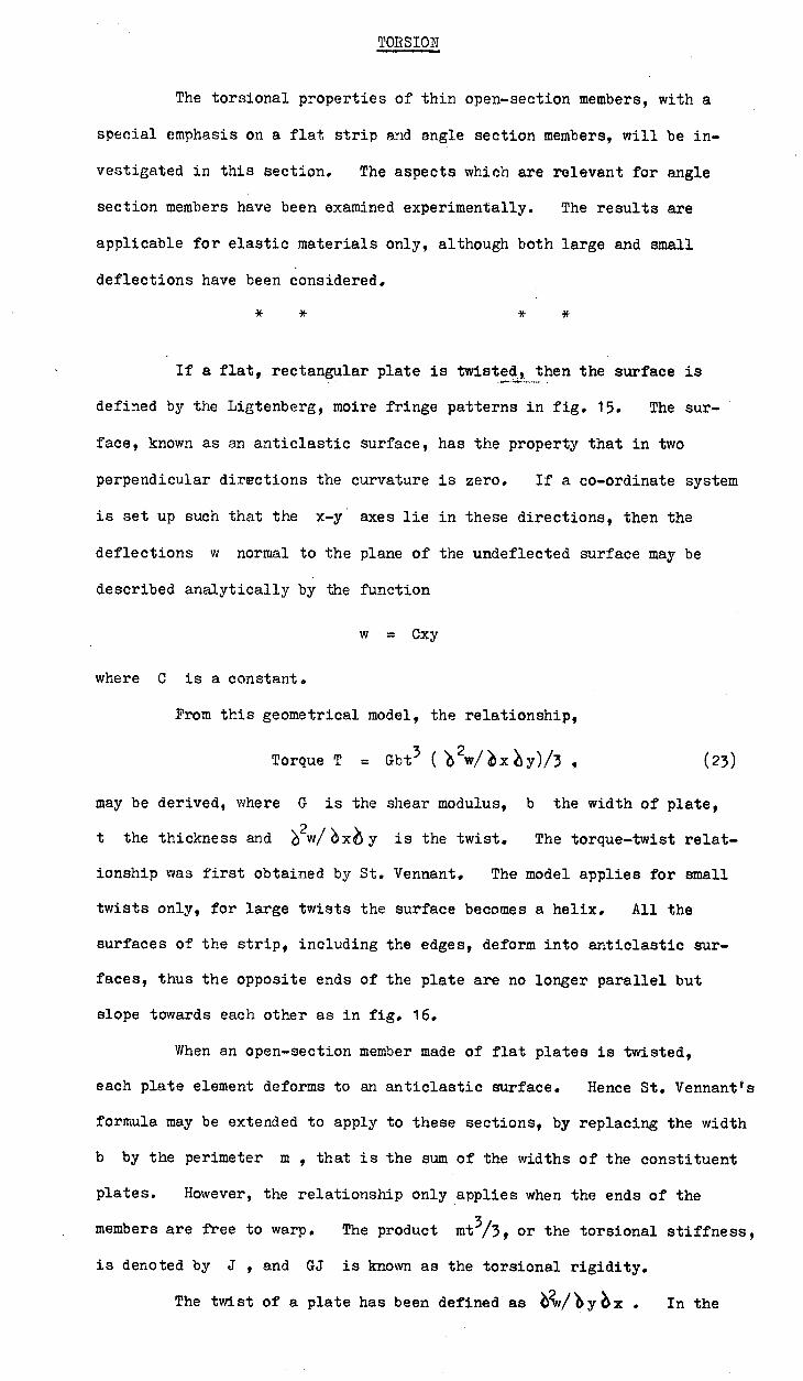
T applied torque 1,4/11y fringes 11.44x fringes
LIGTENBERG FRINGES OF A TWISTED PLATE, AN ANTICLASTIC SURFACE
FIGURE 15
TWISTED SURFACE
FIGURE 16
TORSION
The torsional properties of thin open-section members, with a
special emphasis on a flat strip and angle section members, will be in-
vestigated in this section. The aspects which are relevant for angle
section members have been examined experimentally. The results are
applicable for elastic materials only, although both large and small
deflections have been considered.
If a flat, rectangular plate is twisted then the surface is
defined by the Ligtenberg, moire fringe patterns in fig. 15. The sur-
face, known as an anticlastic surface, has the property that in two
perpendicular directions the curvature is zero. If a co-ordinate system
is set up such that the x-y axes lie in these directions, then the
deflections w normal to the plane of the undeflected surface may be
described analytically by the function
W = CXy
where C is a constant.
From this geometrical model, the relationship,
Torque T = Gbt 3 ( ;1 21NR)x!,y)/3 1 (23)
may be derived, where G is the shear modulus, b the width of plate,
t the thickness and Ww/xey is the twist. The torque-twist relat-
ionship was first obtained by St. Vennant. The model applies for small
twists only, for large twists the surface becomes a helix. All the
surfaces of the strip, including the edges, deform into anticlastic sur-
faces, thus the opposite ends of the plate are no longer parallel but
slope towards each other as in fig. 16.
When an open-section member made of flat plates is twisted,
each plate element deforms to an anticlastic surface. Hence St. Vennant/s
formula may be extended to apply to these sections, by replacing the width
b by the perimeter m 9 that is the sum of the widths of the constituent
plates. However, the relationship only applies when the ends of the
members are free to warp. The product mt 3/3, or the torsional stiffness,
is denoted by J , and GJ is known as the torsional rigidity.
The twist of a plate has been defined as 6210•yex . In the

partially built in support, fringes curved due to warping of cross section.
WARPING OF A TWISTED I-MEMBER
FIGURE 17
LIGTENBERG FRINGES OF A TWISTED CANTILEVER STRIP
FIGURE 18
-

- 25 -
case of a member where the cross-section rotates, in an undeformed state,
then the twist is independent of the y ordinate. If 0 is the rot-
ation of the cross-section relative to some point, usually the shear
centre, then the twist is lqic/,6 x 9 where x is the abscissa measured
along the member. It is important to realize that both the torque and
the rotation must be considered relative to the same point.
For some composite sections the cross-section does not remain
plane, because the ends of each plate are no longer parallel. As an
example consider the cross-section of an I-beam which is shown in fig.
17. The cross-section is said to have warped. When the member is
restrained in some way to force plane sections to remain plane, or is
twisted with varying twist, then longitudinal stresses and shear stresses
are developed in the member. These stresses modify the torque-twist
relationship to
GJ x + Cw 00/ e x39 (24)
where Cw is a warping constant. Reference may be made to one of the
references at the conclusion of this section for the derivation of the
relationship.
The following work is concerned with equal leg, angle-section
members; for these members the shear stresses do not effect the torque,
hence the parameter Cw is zero. However, it should be pointed out
that secondary warping does occur, as the crcss-section of each leg of
the angle warps and deforms into an anticlastic surface. The effect of
the secondary warping can be noticed when a flat strip, which is built in
at one end, is twisted. Near the built-in end, the cross-section is
partially restrained against warping and the twist decreases. One
could consider a fully built-in cantilever as one in which the end did
not warp, and hence the twist is zero. From the Ligtenberg fringes in
fig. 18 it can be seen that this is a very local effect.
Bleich derived an expression for the torque of an equal leg,
angle-section member involving the secondary warping of each leg using
an energy approach. He gives
= GJW:sx + (210 -0 3 e30/b x3/144 .
In this thesis, the author derives the same expression by considering

0.01 0.02 0.03 0.04
large twist mathematical model
X experimental point small twist
mathematical model
////
;-1 0 slope = GJ = 20/0.03 = 650 ,- -p calculated value = 640
twist per unit length
TORQUE TWIST CURVE OF A 2" x 2" x 0.05" ANGLE-SECTION MEMBER
FIGURE 19
slope = 4/0.03 = 330 psi
.003 .006 .009 .012
twist
TORQUE TWIST CURVE OF A 2" x 0.05" RECTANGULAR SECTION
FIGURE 20
torq
ue(in.
1

- 26 -
the bending stiffness of the legs of the angle. For any section with
primary warping the secondary warping may be neglected.
The torque twist relationships both for a flat plate and for an
angle member are shown in figs 19,20 and the elastic constants of prop-
ortionality are evaluated.
For large twists, the torque-twist relationship of an angle-
section member deviates from a straight line, although the material is
still elastic. 1
This phenomena has been investigated by Cullimore, and
2 Gregory, and it was found to be due to the development of longitudinal
strains arising from the deformations out of the plane of the model.
During twist, straight lines across the leg of the angle remain straight.
Therefore the first component of the strain, the derivative of the dis-
placement in the direction of the axis of the member with respect to
the ordinate in this direction, is linear across the leg.
Consider an angle section member which is deforming such that
is the rotation of the cross-section about the shear centre. Let r
be a radial ordinate measured from the shear centre. Then the strain
( due to twisting is
= r2 (:1 0/kx) 2/2
and, as straight lines remain straight, the total strain is
= A + Br + r2 (/)95/bx) 2/2 ,
By considering the equilibrium of axial forces and moments, the values
of A and B can be determined. The expression for the strain is
re b 2/12 - br/2) 9 (25)
where b is the leg width of the angle. Geometrically, the strains
mean that the member not only twists, but also bends. Notice that
there is a line which remains straight; it is not the line of shear
centres. Gregory3has Shown that the derived results are independent
of the point chosen as the origin of the coordinate system.
The longitudinal strain of an angle-section cantilever
Ref. 1 M. S. G. Cullimore & A. G. Pugsley "Torsion of Al Alloy Struct- ural Members", Aluminium Research Development Association Report No. 9.
Ref. 2 M. S. Gregory, Australian Journal of Applied Science, Vol 11,
3 Nos. 1 & 2, 1960, Vol. 12, No. 2, 1961.

0004
1.5 2 radial ordinate r (in)
-.0002 x experimental point
I 0.5
STRAINS IN A TWISTED ANGLE SECTION MEMBER b = 2", t = 0.05", L = 11.5"
FIGURE 21
direct stress twisting stress
bending stresses
FIGURE 22

- 27 -
experiencing a twist were measured with Huggenberger strain gauges.
The results obtained are given in fig. 21, where they are compared with
•the results estimated by the previous mathematics. In this experiment
a "built-in" cantilever was used, but the strains were measured where
the twist was constant. The region was found using the Ligtenberg
apparatus.
For a section in which warping is important the torque twist
relationship for a small twist is
= G‘M 0/6 x c 1 e 3psbx3
When large deflections are considered, two more terms must be considered.
The first is derived in the same manner as for an angle, C2 ( 0/6 x) 2 .
The second term is due to the shear forces which act along the section
N 9 and is related to the derivative of the longitudinal forces xy
The form of this term is C3
1■ 95/6 x ( 6 20/6 x2 ) . The tot-
al torque becomes
= GA 90) x + C 1 630/6 x3 + C 2 ( x)3 695/ax ( 6 20/6 x 2 ) •
(26)
For an elastic material, four local strain readings were used
to determine the loads applied to a member under test experiencing an
axial load, a torque and two bending moments. The twist and bending
deflections were checked using Ligtenberg's apparatus. The four strain
distributions are shown in fig. 22.
This section has aimed at being a concise review of elastic
torsion. It has introduced the terminology and derived the relationships
used by the author. The effect of warping has been included, because,
in the conclusions of the thesis, the methods available for generalizing
the approach developed in this thesis, will be suggested. The section
has also indicated, by means of geometry, the important features, which
the author has included in the following sections on torsional buckling.
References
S. P. Timoshenko: "Theory of Elastic Stability" McGraw-Hill Book Co., Inc., New York.
H. Wagner: "Torsional Buckling of Open Sections" Technical Memorandum No. 807, U.S. National Advisory Committee of Aeronautics 1936.

-28—
H. Wagner and W. Pretscher: "Torsion and Buckling of Open Sections" Technical Memorandum No. 784, U.S. National Advisory Committee of Aeronautics 1936.
Weber: "Die Lehre der Drehungsfestigkeit" Forschungs beiten auf dem Geibiete des Ingenieurswesens, Heft 249,
V. Z. Vlasov: "Thin Walled Elastic Beams".

S shear centre C centroid
leg width b
radial ordinate
///
b/
outstanding leg
/ / I
torque T
bending moments, rotation
axial load P
normal deflections w
thickness t
dimensions co-ordinates
deformations applied forces
NOTATION ASSOCIATED WITH AN ANGLE- SECTION COLUMN.
FIGURE 23.

COLUMNS
Three mathematical models will be developed in this chapter to
describe the behaviour of columns. These models will describe the
local buckling of the column under a uniform axial load and a linearly
distributed end moment, provided the cross-section does not distort.
The second part of the chapter deals with eccentric loads which cause the
cross-section to distort.. The treatment given results from work on
angle-section columns, loaded through one leg by a sJaLle bolt connect-
ion.. The effect of the longitudinal stress distribution, produced by
loading the column through a bolt, has also been estimated using a
"partial energy" approach.
LOAD APPLIED THROUGH A BASE PLATE
The first loading to be considered is an axial load, uniformly
distributed across the cross-section. Simply supported end conditions
are assumed, that is the rotation, the torque, and the moment, are zero
at each end of the member.
The notation associated with the problem is p, q are the co-
ordinates about principal axes of the cross-section. The x, y and r
coordinates are associated with one leg of the angle. The ordinate y
is measured across the leg from the root of the angle, the abscissa x
is measured along the line of shear centres of the member from one end of
the member, and the r ordinate is a radial ordinate measured from the
shear centre. The displacements in the x and y directions are u
and v respectively, and the displacements normal to the x-y plane
are w The properties of the angle are leg width b thickness t,
and length L • The notation is defined also in figure 23.
Experimental Work
The experimental models used to measure the deformations were .
made of perspex; the dimensions were: leg width 4", length 8" and thick-
ness 1/8". These members were loaded through their centroids using a
system of ball bearing supports as shown in fig. 24. The deflections
w normal to the leg were measured using the Ligtenberg Moire method.
The fringes obtained are shown in fig. 25.
In the experimental work, the ideal pin-ended conditions were

An angle-section column deforming under a uniformly distributed axial load. Note an approximate analytic function describing the shape is
w = at cos nx/L .
FIG. 24
(a)
(b)
Ligtenberg fringes for one leg of an angle-section column deforming into the shape shown in Fig. 24. The root of tha angle is on the right (a) dw/dx (b) dw/dy. The quality of the fringes is the same as obtained forall experimental work.
FIG. 25
- 30 -
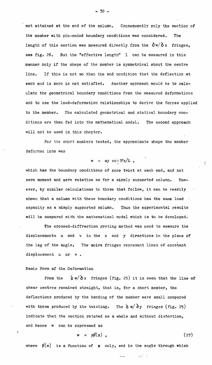
not attained at the end of the column. Consequently only the section of
the member with pin-ended boundary conditions was considered. The
length of this section was measured directly from the 6w/eix fringes,
see fig. 26. But the "effective length" I can be measured in this
manner only if the shape of the member is symmetrical about the centre
line. If this is not so then the end condition that the deflection at
each end is zero is not satisfied. Another approach would be to calc-
ulate the geometrical boundary conditions from the measured deformations
and to use the load-deformation relationships to derive the forces applied
to the member. The calculated geometrical and statical boundary con-
ditions are then fed into the mathematical model. The second approach
will not be used in this chapter.
For the short members tested, the approximate shape the member
deformed into was
= ay cdtTrx/L ,
which has the boundary conditions of zero twist at each end, and not
zero moment and zero rotation as for a simply supported column. How-
ever, by similar calculations to those that follow, it can be readily
shown that a column with these boundary conditions has the same load
capacity as a simply supported column. Thus the experimental results
will be compared with the mathematical model which is to be developed.
The crossed-diffraction grating method was used to measure the
displacements u and v in the x and y directions in the plane of
the leg of the angle. The moire fringes represent lines of constant
displacement u or v .
Basic Form of the Deformation
From the sw/bx fringes (fig. 25) it is seen that the line of
shear centres remained straight, that is, for a short member, the
deflections produced by the bending of the member were small compared
with those produced by the twisting. The fringes (fig. 25)
indicate that the section rotated as a whole and without distortion,
and hence w can be expressed as
w = 0(x) , (27)
where 9f(x) is a function of x only, and is the angle through which

effective length 1
AB is the line of shear centres
LIGTENBERG blOy FRINGES FOR ONE LEG OF AN ANGLE -SECTION COLUMN
FIGURE 26
CROSS DIFFRACTION GRATING FRINGES, LINES OF CONSTANT DISPLACEMENT Cu, v)
FIGURE 27.

- 31 -
the section has rotated. The movement of the centroid of any section
with x constant, under these conditions was b/(2 r7)0(x) . From the
fringes for u and v it was found that horizontal lines, that is lines
with x a constant, remained straight during deformation and /.6x
was much greater than e v/2) y o In algebraic terms u and v were
linear in y and x respectively.
First Mathematical Model
In the first mathematical model, all the internal stresses will
be assumed to be small compared with the twisting moment per unit length,
which is given by the expression
m = D(1 - 1) ) xy
where D is the flexural rigidity and is Poisson's ratio. The
applied longitudinal forces per unit length Nx are assumed to be con-
stant and invariant with the deformations,
Nx
P/A
where P is the total axial load and A is the cross-sectional area.
The longitudinal forces have a component in the direction of the w de-
flections, which is equivalent to a shear force per unit length Q x act-
ing across the leg of the angle
Q = N v0) x P/A 6w/6 xo x x
The equation of torque equilibrium on a plane with x constant is
jrQx r dA + fMxy dA =0 9 A A
or in terms of the deflection w
P/A ) w/ x r dA + )(D(1 - 1) ) 1 2v7/ f3( y dA 9 (28)
which simplifies to the differential equation
GJ14/4?$x (PIp/A) 4/6 x = 0 (29)
when the functional form of equation 27 is used. The torsional stiffness
J equals 2bt 3/3 , the polar moment of inertia about the shear centre
I equals 2b 3t/3 and G is the elastic shear modulus. The strut
remains in the undeformed state for all loads except the load
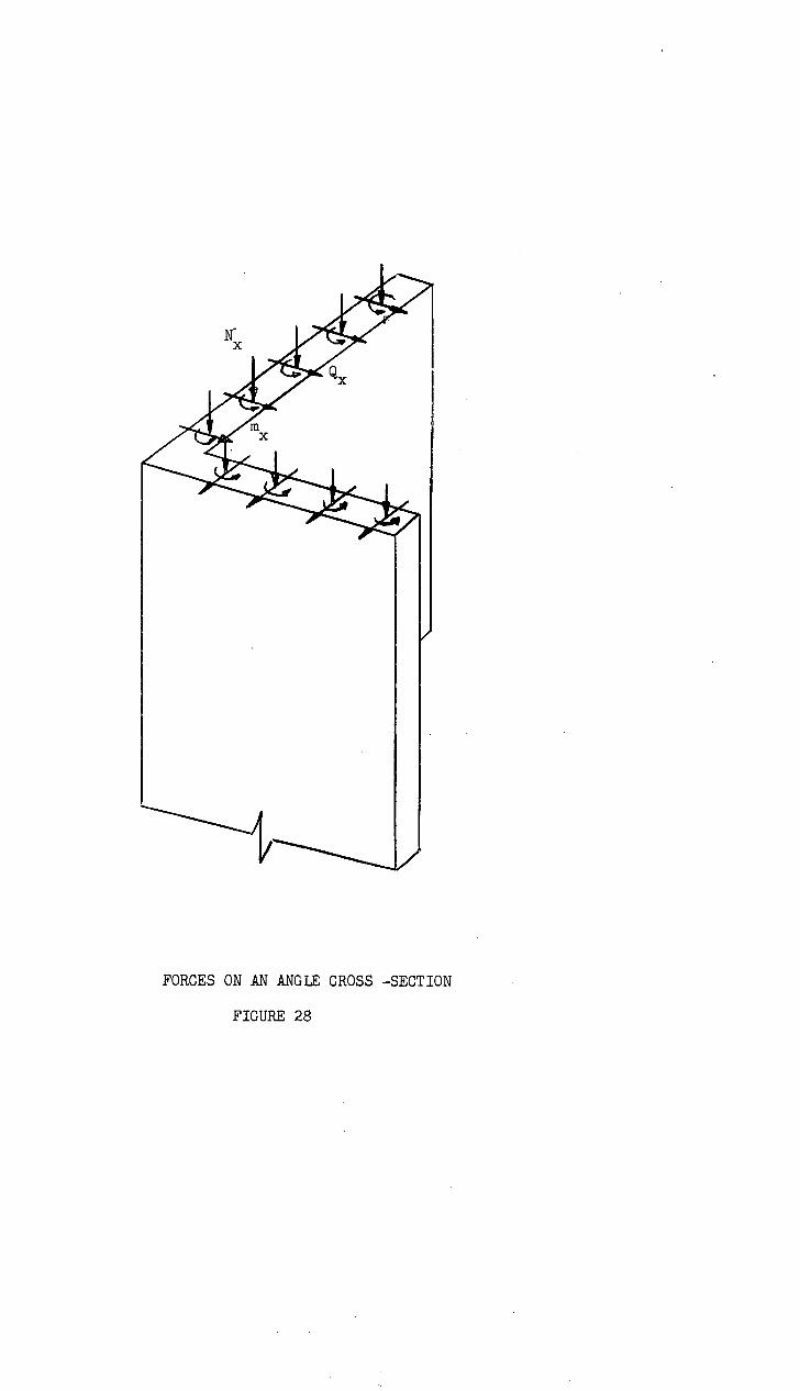
FORCES ON AN ANGLE CROSS -SECTION
FIGURE 28

-32-
perit = GJA/I p 9 ( 3o )
at which load the deformations are indeterminate.
Second Mathematical Model
The experimental work has determined the deformations and not
the shape of the member. In setting up the equations of statical
equilibrium the shape is important. The initial shape is taken to be
u = w = v = 0 0 The mathematical model has as its basis the dis-
placements or deformations u, v and w ; where u is linear in y,
v is linear in x and w = 0(x) . If the problem is limited to
one of small deflections the change in curvatures K x and K of the
leg, consistent with the specified deflections are
Kx
= $2w/6x2
K = 2wA y2
and the change in twist, or torsion, is
K = 2w/ex y = x 0 xy (31)
From the expressions for u and v , the first approximations of the
longitudinal strains are
= u/6 x = (py + r)h(x)
and (32)
= tv./ et y = ( Sx + t)j(y)
where p, r, s, t are parameters. and h and j are functions.
Internal Stresses
The problem is further restricted in that the load-deformation
relationship is taken to be linear, that is the material is elastic.
When this is so the moments per unit length mx m and m required xy
to maintain the deformations expressed in equation (31) are:
m = Dy 20/ x2
m = D y 1, 2r:6/ x2 and (33)
m = ( 1 -1) )D x xy
where the flexural rigidity D denotes Et 3/12(1 - 1; ) 2 . Using the
expressions (32) for the longitudinal strains the longitudinal forces
per unit length acting on the central plane of the leg becomes

- 33 -
Nx = Et(cy + d)q(x) 0
(34)
In order to determine the other internal stresses the statical
equilibrium of an element of the leg must be studied. When an element
of the leg, thickness t, and defined by the planes x 9 x + dx y 9
y + dy is considered, the following equations are obtained (see fig.
29).
Force equilibrium in w-direction:
0Qx/le y + obQ3r/ x =
moment equilibrium in w-x plane:
Qx = 1111)P) x 5111xle Y Nx x Nxy Y (35)
and moment equilibrium in w-y plane:
Qy = 6my/ y - 6 mxy/ x - Ny y N3c3r ) x o
The equilibrium equations (35) in conjunction with the load
deformation relationships (33) give an expression for the shearing
force per unit length,
Qx
- Dy 3Ø/è x3 - Nxy 95/2:4 x - Nxy91 • (36)
Applied Forces
As the axial force is applied through the centroid of the
section of the member, the only applied end force is an axial force P
and hence the resultant forces on a section D-D (see fig. 23) with
x constant are:
Axial force 1
moment about minor axis • • 0 Mp = OPb/2
(37) moment about major axis • • • • M
Q = 0
and torque about x-axis • • • T = 0
The forces on any Section must be balanced by the stress
resultants on that section. These are obtained by integrating the in-
ternal stresses. When three of these forces, the axial thrust and two
moments, are considered the following three equations are obtained

- 34 -
qdA = 0 Pb/2 7 A
MQ = Nx pdA = 0
(38)
A
and
P .INx
dA 9
A
where IdA denotes the integral over the whole section. From equations
(38) the values of the parameters, c and d in the functions des- \ A
cribing the longitudinal forces per unit length in both legs are
determined.
Nx1 = tP/A 344/41)2
(39) and
Nx2 = tP/A - 3P0y/4b
2
The fourth force, the torque, is balanced by the moment of the internal
stresses about the shear centre. The moment of the internal stresses •
is independent of the point about which it is taken. The shear centre
was chosen so that the shear forces N need not be evaluated. The xy
torque balance gives
dA -ydA - yvvP)3T dA = xy x xy
A A A
0 (40)
When the expressions for m 9 Q 9 and N in equations xy x
(33), (36), (39) are substituted into the equation (40) the differ-
ential equation is obtained as
GJ 0/6 x - D 630A x - P )0A x = 0
in which G is the shear modulus, J the torsional rigidity = 2bt 3/3
and I is the polar moment of inertia = 2b 3t/3 . After rearrangement
the equation becomes
(P/2Db - GJt/DIp)e0/ x = 0 • (41)
A solution of the mathematical model is
w . an sin nIfx/I,
where n is an integer, as it satisfies both the differential equation
(41) and the boundary conditions: Mp = MQ = T = 0 and w = 0
at x = 0 and x = L • But there are two conditions on the
solution: either an = 0 or

- 35 -
-(nIT/L) 3 + (Pnt/AD-tGJ/DI )7/L = 0
(42)
Hence equation (41) has an infinite number of eigenvalues of P 9 given
by (42), corresponding to an infinite number of eigen functions
wn = any sin n irx/L n = i(i) co .
Energy
When a differential cannot be solved explicitly an approximate
solution can often be found using a weighted integral of the differ-
ential equation. The expression for the weighted integral can be
obtained from the differential equation. In this case the differential
equation is multiplied by 'o2Ø/'x2 and integrated twice with respect
to the x variable to give
L 2Ø/ 2 )2( 0J/2 0 piRixy N ( die x) 2 0
DI /2t (1.1 x P/ 10 P )0
(43)
which is identical to the energy expression
Lb / .2w/
2 \2 /. 2\2 u D - 2 / - ..1)( 2
14,A x2 >12w/ y2 f j 2 k 6 6 x + o w / 4) y ) 0 v 00
Lb
( eINA y) 2 ) dy dx + f ir Nx
w/ x) 2 dy dx 9
0 0
(44)
when the functional form and the loading conditions are applied and the
expression is integrated with respect to y • Thus the minimization of
the energy expression is equivalent to the least squares method of
averaging the differential equation.
Initial Shape
No physical membcr is initially straight, and as the mathematical
model is non-linear, it is expected that the behaviour of the member
depends upon the initial shape. When the initial shape is w = w 0
the differential equation must be modified as the moments per unit
length depend upon the change in curvatures and the change in twist:
b2 (w - wo )/e. y2 , 2 (vi - wo,)/6 x2 and w0 )/
respectively. When these corrections are included, equation (41)
becomes
)3 (91 - 1/(0)hx3 + Pt/DA Ø/x - GJt/I p grAx - )0(3,/ x) = 0 • (45)

300 calculated critical load
200
experimental point 100
0.01 0.02
maximum slope
0.03
0.04 0.05
6
LOAD-DEFORMATION FOR AN 8" x 4" x 4" x 1/8" ANGLE-SECTION MEMBER
FIGURE 30
slope = 1/Pcrit = 1/300
.001 .002 .003 .004 .005
maximum dw/dx
SOUTHWELL PLOT FOR THE ABOVE MEMBER
FIGURE 31
AB original state A'B' deform state
Strain = eu/2tx + -1-Ww/6x)2
U +u/16x dx
A
FIGERE 32

- 36 -
The initial shape can be expressed as an infinite series of the eigen
function of the differential equation (41),
0 =a0 sin nirx/L 0 ,
This is possible as the eigen functions are orthogonal. The solution
of the differential equation is then
co .E an
sin nlrx/L n=1
with the coefficients an given by
an = aOn (1 - F/Pn) n = 0(1) CD. (46)
In the neighbourhood of P 1 the first term of the series predominates
and the shape is approximately 0 = a l (1 - P/P 1 ) sinInc/L P1 is
the lowest eigen value, which is called the critical load and is calc-
ulated using
1 —/
= 2(Db 2/L
2 + GJbt/I )
This mathematical model buckles in the Eulerian manner like a
simple column. If the member is initially straight it can be in either
one of two states, zero deflection or indeterminate deflection. The
second state occurs only for well defined loads P n . When initial
shape is included, the load deflection relationship of the mathematical
model approaches the lowest critical load asymptotically (fig. 30).
Equation (46) justifies the use of the Southwell plot, that is plotting
(w - wo )/P against w - wo . The slope of the graph is the inverse of
the first eigen value or critical load. The Southwell plot was used
to evaluate the critical loads of the experimental members (see fig.
31).
op
Third Mathematical Model
In the first model the longitudinal strains on the centre plane
of the leg were taken as = u/ x . In the model to be studied
next, the shortening due to bending is also tol.be considered. The
approximate expression for curvature is still to be employed as the
twists measured experimentally are not large enough to justify the use
of more complex expression. From fig. 32 it can be seen that the bend-
ing deflections w modify the longitudinal strain to give
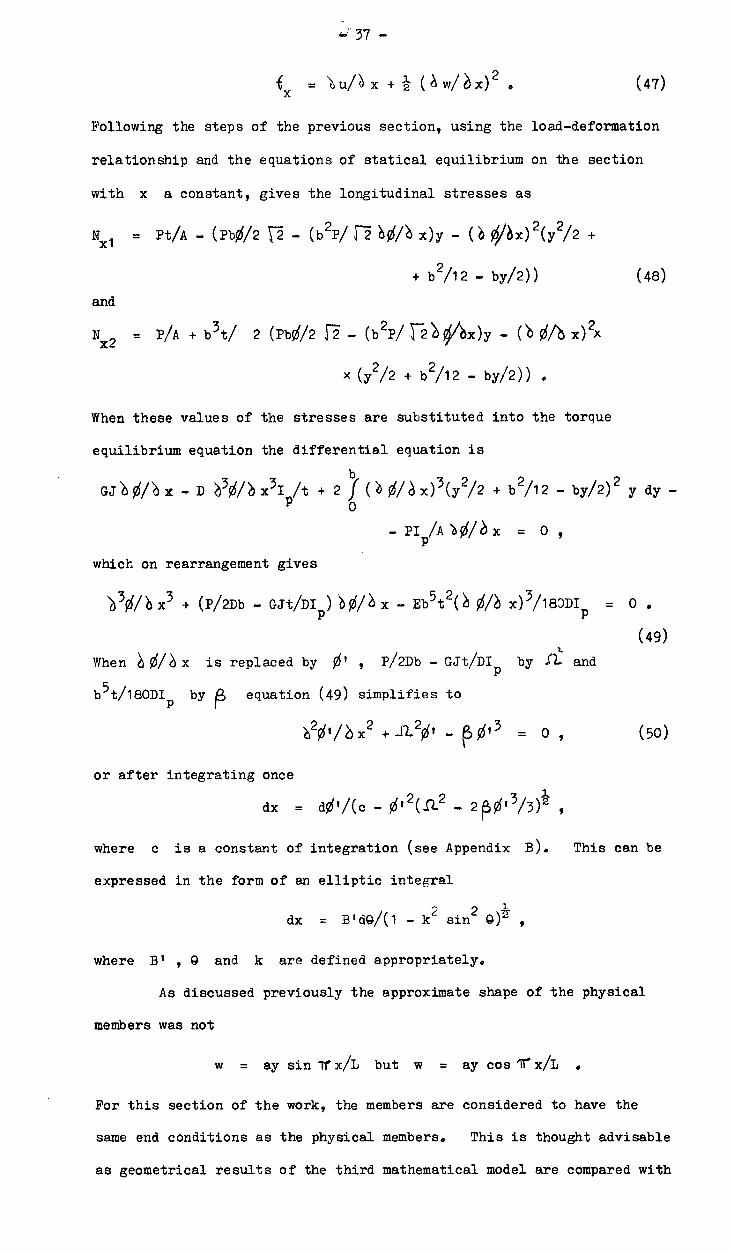
,;37—
= uP x + ( w/ 3c) 2 (47)
Following the steps of the previous section, using the load-deformation
relationship and the equations of statical equilibrium on the section
with x a constant, gives the longitudinal stresses as
1 = Pt/A - (Pb0/2 - (b 2p/r 1-.27 x)y _ 4/6x) 2 (y2/2 x
+ b 2/12 - by/2))
(48) and
Nx2
P/A + b 3t/ 2 (Pb0/2 - (b 2P/ 1-20x)y - 0 x) 2x
x (y2/2 + b2/12 - by/2))
When these values of the stresses are substituted into the torque
equilibrium equation the differential equation is
Ge1?“0x - D 3g5/) x31 /t + 2 j( ( 0/d x) 3 (y 2/2 + b 2/12 - by/2) 2 y dy - P 0
- PI /A 4/6 x = 0
which on rearrangement gives
) 30R) x3 + (P/2Db - GJt/DI ) x - Eb5t 2 ( x) 3/183DI = 0
(49) When a 95/, x is replaced by 0' P/2Db - GJt/DI by Si: and
b 5t/180DI by equation (49) simplifies to
:120 1 /6 3c 2 ji. 20 1 01 3 = 0, (50)
or after integrating once
dx = dØ'/(c - 0' 2012 - 2013/3Y2 9
where c is a constant of integration (see Appendix B). This can be
expressed in the form of an elliptic integral
• 2 \-& dx B 1 40/(1 - k sin 8) - 9
where Bt Q and k are defined appropriately.
As discussed previously the approximate shape of the physical
members was not
w = ay sin ir x/r, but w = ay cos
For this section of the work, the members are considered to have the
same end conditions as the physical members. This is thought advisable
as geometrical results of the third mathematical model are compared with

2
300
V
1 Euler small deflection curve 2 Approximate large deflection, initially
straight curve(K = approx.V2) 3 Large deflection,initially straight
curve 4 approximate, larfm deflection, initially
crooked curve (K=1172) 5 Measured curve
20
'0 ozi 0
100
.01 .02 .03 .04 .05
twist
dy
LOAD - DEFORMATION CURVE FOR A COLUMN
FIGURE 33

- 38 -
the geometrical results of the physical model.
The functions 0 1 = B sin 2Kx/L satisfies the boundary con-
ditions and when substituted into the differential equation (50) gives
B(2K/i) 2 (2k2sn32Kx/L - (1 + k2 )sn 2Kx/L) +2Ber! 2Kx/i - pB 2sn32Kx/L = 0
4K is the period of the sn function and K is equal to the complete
elliptic function, 1772 22 \--1-p K = (1 - k sin 17 ) -dy0
0
(see Appendix B for properties of sn z ). By equating the coefficients
1 / N of sn(210r./L) and sn3 (2Kx/L) two conditions are obtained:
2(2KkL) 2 -13B2
= 0
(51)
and (1 + k2 )(2K/L) 2 =J2. 2 0
These two equations in conjunction with the k-K relationship
is solved for a load-deformation relationship (P, B) ; the form of which
is shown in fig. 33. For small deflections an approximate load-
deformation relationship is obtained by combining equations (51) and
using the fact that K = ir/2 for small k • Hence
P/Db2.- GJt/I D b5 .0 2/3b0DI - (1r/L)a o /
(52)
For P <2.0b(1r/L) 2 + GJtb/ip) the deflection is zero, which is ident-
ical with the simpler model. However, the third model predicts a
unique deflection for each load, which is in contrast to the second
mathematical model which buckles in the sense that the deflections are
indeterminate at the critical load. Thus it appears that Eulerian
buckling is a property of the mathematical model and not the physical
member. In this respect the second model bears the same relationship
to the first model as the "elastica" does to Euler's column. The math-
ematical model of the elastica includes a more exact expression for the
curvature of the column.
In order to calculate the magnitude of this effect we shall
1" calculate deflection for a 4" x 4")( perspex angle member, 8" 8
long, with E = 480,000 p.s.i.and = 0.3 • For P = P . + 100 crit
B 2 = 120 x 8 )( 100/(480,000 X 64) = .00313
and hence = 0.56 rads/in.

- 39 -
The maximum deflection can be estimated when it is assumed that
the shape is
. By (sinirilli + 1) and Sc6/2) x = B TO, cos 'Tr
The assumption is of the same order as that made in obtaining the approx-
imate equation.
Then
w = 2 * 4 4 0056 V 8/Tr
. 1.14 in.
When P - Pcrit = 50 the deflection w is 0,808 inches.
The two simultaneous equations (51) can be solved by trial and
error to give the true load deflection relationship. For the same
member
and
(9,
41.2
=
=
' Eb t
2 /180DI =
P/(2Db) GJt(6(1
92.2
. 0.00144P - 0.262 .
Using the same deflection as above, B2 = 0,00316 9 equation (51),
8(Kk/L) 2 = B2/2 9 gives
k2 = 0.59 and K2
= 3074 .
With these values the second equation, (1 + k2 )4K 2/1, 2 = J12 9 becomes
2 = 0.372
or 0.00144P = 0.372 + 0.262 9
which reduces to
P = 440 lbs or P - Pcrit = 158 lbs.
Other points on the true load deflection curve have been calculated by
the same method. The true curve is plotted with the approximate curve
on graph 33. As can be expected the two curves agree in the region of
small deflections, the region in which the assumption holds.
The third mathematical model does not include the initial shape
of the member. The importance of initial shape can be appreciated
from the load deflection curve based upon the small deflection model.
1" This curve is plotted on graph 33 for a 4" x 4" 8" X perspex

- 40 -
model with an initial twist of 0.001 in. The differential equation
(49) can be modified to allow for any initial shape. The shear strains,
the plate bending strains, and the longitudinal strains due to twisting
depend upon the change in shape. When the initial shape is
w0 = B
the modifications give
3(91 00)Ax3 + F10/6 x/2Db GJt/DIp (95 - 00)/ x
b5t (95 - (,0)/x x/180DIp = 0
or
2 (0 2 - 00 )h, x + IVO - 1)2'0 - - Øt)2Ø = 0. (53)
The differential equation cannot be solved easily, if at all, and con-
sequently an approximate solution is obtained. It can be expected that
the shape of the member changes with the load, as it did for the init-
ially straight member. To obtain an approximate solution it is assumed
that the change in shape is not appreciable, and that the initial shape
is of the same form as the deformations. Take
w0Ax = B
0y sn 21(x/L and w/ x = By sn
As for the initially straight member, two equations are obtained when
the values of c?0:41c and0 x are substituted into the differ-
ential equation (53). These are
2k - B0)(2K/L) - p(B - Bo)B . 0 2 / / .2 (54)
and (B B0 )(2K/1) 2 (1 + k2 ) +11 1B - SV(B - B0 ) = 0 ,
The value of K is assumed to be Tr/2 , which is in keeping with the
earlier assumption that the shape does not change to any extent.
Physically, these assumptions mean that the shape is approximately
described by
w/)3 x = By sin Trx/li
Under these conditions, the above two equations (54) combine to give
AgBAB - B0) = 11" + ( 1T/L) 2 + pB(B - B0)/2
(55)
For a 4"x 4"x Ti 8" perspex model with an initial deflect- 1"
ion of B0 = 0.001 rads./in. this becomes
0.00144B/(B - B 0 ) = 0.416 + 46.1B(B - B0) .
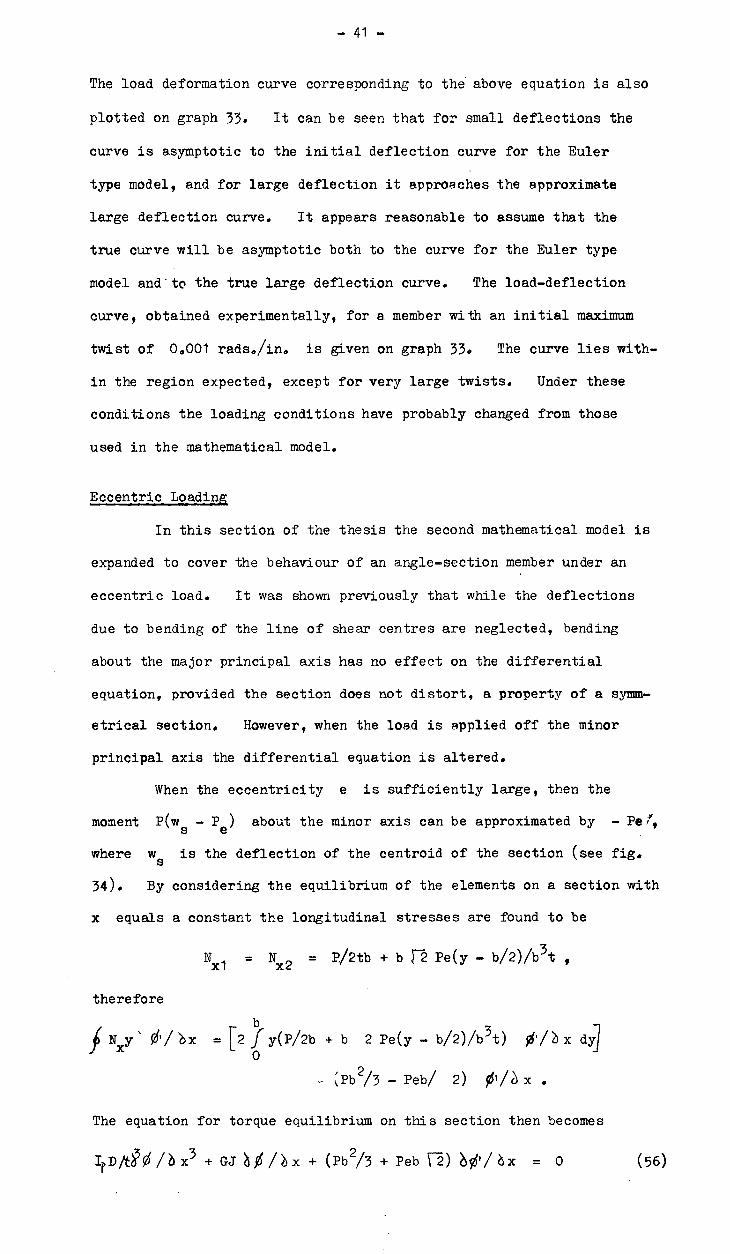
— 41 —
The load deformation curve corresponding to the above equation is also
plotted on graph 33. It can be seen that for small deflections the
curve is asymptotic to the initial deflection curve for the Euler
type model, and for large deflection it approaches the approximate
large deflection curve. It appears reasonable to assume that the
true curve will be asymptotic both to the curve for the Euler type
model and to the true large deflection curve. The load—deflection
curve, obtained experimentally, for a. member with an initial maximum
twist of 0.001 rads,/in, is given on graph 33. The curve lies with-
in the region expected, except for very large twists. Under these
conditions the loading conditions have probably changed from those
used in the mathematical model.
Eccentric Loading
In this section of the thesis the second mathematical model is
expanded to cover the behaviour of an angle—section member under an
eccentric load. It was shown previously that while the deflections
due to bending of the line of shear centres are neglected, bending
about the major principal axis has no effect on the differential
equation, provided the section does not distort, a property of a symm-
etrical section. However, when the load is applied off the minor
principal axis the differential equation is altered.
When the eccentricity e is sufficiently large, then the
moment P(ws
— Pe) about the minor axis can be approximated by — Per,
where ws
is the deflection of the centroid of the section (see fig.
34). By considering the equilibrium of the elements on a section with
x equals a constant the longitudinal stresses are found to be
\/ Nxl
= Nx2
= P/2tb + b Pe(y — b/2)/b 3 t 9
therefore
Nxy = [2 f y(P12b + b 2 Pe(y — b/2)/b 3t) x dy-1 0
- IL1D 2/5 — Peb/ 2) 0 1 /x .
The equation for torque equilibrium on this section then becomes
I DA x3 + GJ /) x + (Pb 2, 3 + Peb ) Ø'/x = 0 (56)

eccentricity e
stable
poi
nt
-1 -2 -3 -4 1
eccentricity about the minor axis e (ins.)
CRITICAL LOADS FOR AN ECCENTRICALLY LOADED 8" x 4" x 4" x 1/8" PERSPEX MODEL BASED ON THE THIRD MATHEMATICAL MODEL
FIGURE 34

-42-
and from this
w = ay sin n
and
Pcrit = =2(Db( 1r/L) 2 + GJbt/Ip)b/(b + 3 rb) •
13 1 (57)
See graph on fig. 34.
From fig. 34 it can be seen that there is a good agreement
between the load capacity of the physical member and the mathematical
model. When the eccentricity is - 13/3 77 the critical load is in-
finite and the member is stable. If the eccentricity is less than
- b/3 the mathematical model predicts that the member will buckle
in tension but not in compression. At this stage a member has not
buckled in tension as the member has failed by another mechanism.
This thesis has only presented the torsional buckling of the whole
member. For some of the models tested with large eccentricities local
compressional buckling occurred under the loading position.
Applied Torque
When a torque T is applied at the end of the column the diff-
erential equation is modified to give
DI /t 31/5/)3c3 + (PI /A - GJ)) 0/6x = T,
the solution of which is
= a sin (kx/L) + TODIp/A - GJ) + C 9
where C is a constant. The boundary conditions are 0 = 0 at
x = 0 and x = L Thus
C =0
and a = - TL cosec (k)/(PI /A - GJ)
The expression for the rotation is
0 = T(x - L (cosec k)(sin kx/L))/(PIp/A - GJ)
and the central rotation is
0c = TL(1 - sec k/2)/2k(PI /A - GJ) 0
(58)
As the load tends to the critical load the parameter k tends to one,
as shown by equation (58); the central rotation approaches infinity.

020 1!
experimental curve
= 0.0048y coslrx/8
y = 4 ins. free edge
.008
y =2 in
004
D 2 x (inch)
-2 ins.
.4
fringe number (Dw/ey)
VARIATION OF THE w/iby• FRINGE PATTERN WITH THE LOAD
FIGURE 36..
(a)?)10y fringes on one leg of an angle-section member, load change 0-120 lbs., (Wly is a function of x only.
(b) y fringes for a load change of 360-480 lbs.
COMPARISON OF THE WERIMENTAL AND THE CALCULATED SHAPE OF A COLUMN WITH A UNIFORMLY DISTRIBUTED AXIAL LOAD
FIGURE 35

- 43 -
/ In the same manner that the relationship between the end slope
of a column and the applied axial load and end moment is used in the
analysis of buckling of frames, the relationship above could be used to
modify the analysis of the buckling of frames out of their plane. The
state of knowledge of the analysis of the instability of frames is given
in Gregory's "Elastic instability - Analysis of Buckling Modes and
Loads of Framed Structures" and his Doctor of Philosophy Thesis sub-
mitted at the University of Tasmania.
It is suitable at this point to discuss the value of the math-
ematical models developed so far. First the shape of the deformed
members is considered. In fig. 35 the measured values of the slope
)w/6 x are compared with the analytic expression
w = ay cos 71' x/L
Theconstant a has been chosen so that the maximum slope values agree.
There is a slight difference in the shape and this can be accounted for
if the analytic expression
w/ x = ay sn 2Kx/L
is used.
For large deformations the functional form, used as a basis for
all the mathematical models, was no longer valid, as the legs of the
angle member began to bow. For large deflections the physical model
deflected into the shape
w = a1 y cos7 x + a 2y2 cos 21rx/L
instead of
w = ay cos ir x/i., •
Note that the physical models do not have simply supported boundary
conditions. For the Ligtenberg fringes and a graph of the twist, see
fig. 36. If a mathematical model were developed, based upon the new
shape, the lowest critical buckling load would be the same, but some more,
higher valued, buckling loads and modes would be introduced.
If there is a component of the shape of the form
w = a1 y cos 11" + a2y2 cos 11"x/L

1" 4" 4" —
8
,
4" 4"
1" 8 11 3 11 3 11 ..... 8
1" 30" 4" 4" —
a
280 300
73 83
435 , 440
185 178
- 44 -
then the lowest or critical load would change and it would depend upon
the ratio of a l to a2 . From the Ligtenberg fringe photographs this
ratio is large and consequently the critical load derived from this shape
is approximately equal to the critical load obtained from the second
mathematical model,.
Another approach to the problem is to consider each leg of the
angle-section member as a plate, as Timoshenko did. Then the leg of
the angle members bows. In fact, the shape of the member depends
upon the size of the member. The critical load obtained by considering
the leg as a buckled plate is very close to the value from the second
mathematical model. The mathematical model developed by Timoshenko
is discussed in fuller detail in the conclusions.
The calculated and measured values of the lowest critical load
are quoted in the table below. All the members tested were made of
perspex. The calculated values are obtained from the second math-
ematical model. For the members tested the first mathematical model
predicts a lower critical load. From the form of the expression for
the critical load, derived in the second mathematical model, it is
sufficiently accurate to use the first mathematical model only for
long members.
Member Calculated Critical Load (lbs) Measured (lbs.)
The maximum error is seventeen percent for the very short
member. The errors for the remaining members are of the order of five
percent. 1"
The critical loads for 8" x 4" X 4" x perspex angle-
section member loaded eccentrically about the minor axis are shown in
fig. 34. The differences between the calculated and measured values
are of the order of five percent. This difference is considered sat-
isfactory, when it is realized that in a practical application the
"effective length" of the member must be guessed, thus introducing an
error of a larger magnitude.

axial load
root of angle section
free edge
--1 )1,176x fringes on the loaded leg
31NrAy frin-ga on the loaded leg
mxy1 H
local Torque T"
Qx2
unloaded leg
loaded leg
W'bx fijjs
'6w/dy frins on the unloaded on the unloaded
leg leg
LIGTENBERG FRINGES OF SLOPE ON HALF OF EACH LEG OF AN ANGLE-SECTION COLUMN LOADED THROUGH ONE LEG
FIGURE 39
THE INTERNAL ACTIONS ON ELEMENTS FROM EACH LEG OF THE ANGLE SECTION COLUMN
FIGURE 40

-45-
Although some of the physical members failed above the critical
load when the material yielded, the author does not suggest that a large
deflection analysis is of value in general practice. This opinion is
based upon two points. Firstly, the displacement is too large to be
tolerated in practice, and secondly, any small lateral load will produce
a large change, both in shape and maximum deflection. In other words,
the members must be considered as physically unstable,
COLUMNS WITH BOLTED END-CONNECTIONS
Earlier work has shown that if an angle-section member is
'loaded eccentrically about the minor axis, then the critical load
increases as the load moves towards the shear centre, and if the column
is loaded eccentrically about the major axis there is no change in the
critical load. These results are true only if the cross-section does.
not distort.
Several aluminium angle cross-section members, bent from alumin-
ium sheet, were loaded through bolts placed at the-centre of one leg as
shown in fig. 38, that is, with an eccentricity of b/2 5- about the major axis. The most noticeable fact about the geometry of the loaded
structure is that both legs no longerundergo the same deflection.. The
loaded leg experiences a much larger deflection than the.unloaded, or
outstanding leg. The ratio of the deflection near the critical load
appears to depend primarily upon the type of root of the angle. Several
perspex models were made with different amounts of glue at the root.
Each had a different deflection ratio. Also the critical load for
this member was much lower than the load given by the mathematical
model based upon an undistorted cross-section. For the overall, or
torsional mode of buckling to occur, the bolt must be tightened suff-
iciently to prevent any local buckling directly under the bolt. The
local buckle was observed in all of the early columns tested.
Ligtenberg moire fringes were obtained for both legs. These
fringes are shown in fig. 39. A straightline across the legs no longer
remained straight. The bcwing is most noticeable in the region of the
bolt. Although in the central portion of the structure the.legs are
not straight, the bow is not appreciable. Hence it appears that the

The mechanism for loading an angle column through one leg. The member is deformed into the elastic buckling mode.
FIG. 37
The shape of a column which has been loaded past the elastic buckling load until plastic deformations have occurred. Note that the triangular mode only forms in one leg.
FIG. 38
- 46 -
difference in the deflection of the two legs is taken up by the opening
of the angle at the root. From the fringes in the other direction,
the x direction, the shape of the central portion is roughly sinusoid-
al, which suggests that the longitudinal stress in the central region
of the member is constant, as is to be expected for members with large
length-leg width ratios. The effective length of the member is
roughly half the total length, as the bolted connections produced
built-in end conditions.
First Mathematical Model
The first mathematical model has the longitudinal stress on the
central plane of the legs constant in the central half of the column,
1/4 < x < 3L/4
the leg remaining straight and the included angle at the root changing.
The shape of the deformations of both legs will be assumed to be of the
same form within the central half of the member, and given by
wl a1 y0 for the loaded leg
and
w2 a2y0 for the unloaded leg
(59)
This model induces a finite moment at the root and zero moment in the .
legs. Naturally the moment is not discontinuous, but as a first
approximation the discontinuous model will be used. It has further
been assumed that the moment at the toot of the angle is linearly
related to change in the angle contained between the legs
‘.= C(al - a2 )0 ' Y
Actually the root of the angle is at a high stress as it will have
high residual stresses from the formative process, and also high
shear stresses due to stress concentration at the corner. These
facts could produce the weakness at the root. The constant of
portionality has been evaluated experimentally, and it would appear
that the constant must be so evaluated for each different type of angle
section member.
As before, only certain equations of equilibrium are satisfied.
Two elements are considered; a strip width b 9 thickness t and
length dx from each leg, see fig0400 When the linear bending theory

-47-
is applied to the bending moment about the major axis the longitudinal
stresses are
Nx1 P/A + My/I 2 TT
PP
and Nx2 = P/A My/I 2 7.
PP.
The shear stress across the thickness Qx are obtained by considering
the internal statical balance. The expression for the shear stress,
Qx = - Dy 304 x3 - NxyW) x - Nxy0 (60)
is derived in appendix A.
The above formula (60) for the shear stresses does not take into
account the rapid change of moment m around the root of the angle-
section member, which produces shear stresses and twisting moments on
the planes, with x constant, in the vicinity of the root of the
member (see fig. 40). In the following analysis, the torque of these
two quantities about the shear centre is combined, and considered as
the one torque, called the local torque. The total local torque is
assumed to vary linearly with the x-ordinate. The torque equilibrium
of one leg of the member gives the value of the local torque at the end
of the member as
L/2 T" = f C(al - a2)0 dx = + (a l - a2 )T' „
0
and thus the distribution of local torque is
+ (a, - a2 )T 1 (L/2 - x)2/1.,
The torque equilibrium for an element from the loaded leg gives
(j( my dy)R x dx + j( Q y dy)/x dx = m dx+(a l - a2)2TIL dx 0 0 x 0 x
When the appropriate expressions for m m Qx and Nx are , xy
substituted into the equilibrium equation the following differential
equation in 0 is obtained,
a DI /2t'00 x4 + a (PI /2A + Peb 4/4 771 - GJ/2) 20/ x2
1 p 1 p• • . pp
= C(al - a2 )0 + 2T 1 (a1 - a2 )/Z (61)
In the same manner the equation for the torque equilibrium of the element
from the unloaded leg gives the differential equation
a2DIp/2t 1 20h x4 + .a2 (PI /2A - Peb 4/4 r /2) 0/2) x2 =
(a, 1 - a2 )0 7 ,27 1:(a - a )/L (62)

- 48 -
We shall assume that the boundary conditions are that the rotation is
zero at x = 0 9 the twist iszero at x = L/2 and the moment is
zero at x = L/4 and 3L/4 . The solution is then
w1 = a1 y(cos (2nrrx/L) - 1)
and w2 = a2y(cos (2ncrx/L) - 1)
If 1 is the effective length, then two linear equations in the
unknowns a 1 and a2 are obtained,
(DI /2t)( Tr/1) 4 - (PI /2A + Peb4 / r-- /1 .2 /4 - GJ/2)( 42 I 1r/) - C 9 4- C PP
4- C 9 (4- DI/2t)( 1r/L) 4 (p/p/2A Peb 4/4 r2 Ipp - GJ/2)(7r/1 C
a 1
a2
= [0] (63)
For the solution to be non-trivial the determinant of theleft-hand side
must be zero, which gives a quadratic characteristic equation- in P
For each value of n there are two solutions for P 9 and, although at
these loads both displacements are indeterminate, the ratio of the two
displacements can be determined. The ratio has two values, one
corresponding to each load. Nevertheless there are an infinite number
of modes and critical loads, as n• can vary from zero to infinity.
The two ratios obtained for the one value of n are linearly
independent, or orthogonal, and, as the functions cos nirx/L + 1 and
coszkifx/L are orthogonal, all the modes are orthogonal and any shape
can be expressed as a unique sum of the modes, such as
co w1 = y E aln(cos nIrx/i + 1) + a2n(cos n1Tx/L + 1) n=1,
OD
and w2 = Y 2: R mnaln(cos n1Tx/L + 1) + R 2na2n(cos nlrx/L + 1) 9 n=1
where aln and a2n are constant and R ln and R 2n are the critical
ratios for the shape cos (nlrx/i) - 1 .
One of the members which was tested was made of aluminium sheet.
having Young's modulus E = 10 psi , and thickness t = 0.65", and
length L = 24" and leg width 4" • For this member the two simul-
taneous linear equations are
(260.6 - 0.394P)a1 - 14382 = 0
and 143a1 + (260.6 - 0.o22P)a 2 = 0
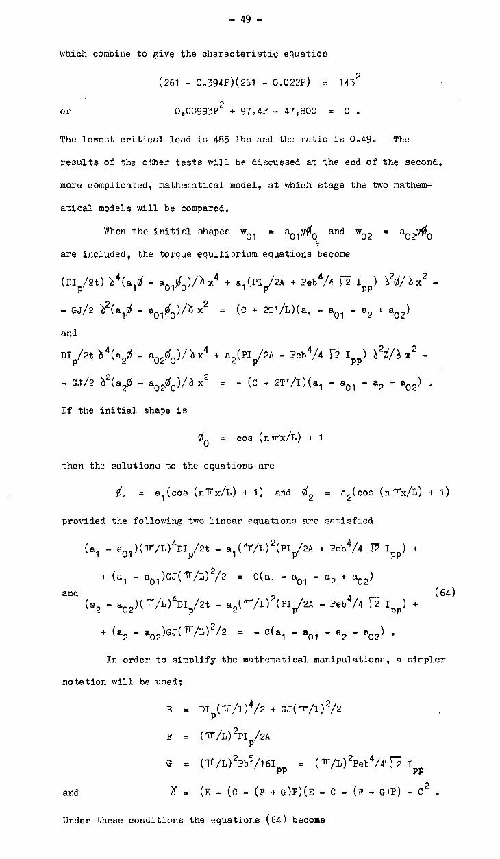
— 49 —
which combine to give the characteristic equation
(261 - 0.394P)(261 - 0.022P) = 143 2
or .
0000995P2 9704P - 47,800 = 0 .
The lowest critical load is 485 lbs and the ratio is 0.49. The
results of the other tests will be discussed at the end of the second,
more complicated, mathematical model, at which stage the two mathem-
atical models will be compared.
When the initial shapes w01
= a01 y00 and wOz = 802700
are included, the torque equilibrium equations become
(DI /2t) 1 - aoi 00 d x4 + a 1 (PI p/2.A + Peb 4/4 1 'pp ) 2$/x2 -
- GJ/2 2 (a 1 0 - a01 00 )/ox2 = (0 + 2V/L)(a1 - a01 - a2 + 802 )
and
DI /2t ) 4 (a2PS - a02 00 )/2) x4 + a2 (PIp/2A - Peb 4/4 F i) 20/e x 2
PP
- GJ/2 b2 (a20 - 8000 )/) x2 = - (c + 2V/1)(a1 - 801 - 82 4- 802 ) '
If the initial shape is
= cos (nTex/L) + 1 0
then the solutions to the equations are
01 = al (cos (nTrx/L) + 1) and 02 = a2(cos (n1rX/L) + 1)
provided the following two linear equations are satisfied
(al - a01 )(Tr/L) 4DI p/2t - a1 (1r/L) 2(PI /2A + Peb 4/4 j i) + PP
▪ (a l - a01 )GAITYL) 2/2 = C(a l 8.01 - a2 + a02 )
(a2 a02 )( 1r/L) 4DIp/2t - a2 (1r/L) 2 (PI p/2A - Peb 4/4 Ti ) pp
•(82 - 802 )Gj("/L)2/2 = C(81 - 801 _82 - 802 ) •
In order to simplify the mathematical manipulations, a simpler
notation will be used;
= DI (11- /1) 4/2 + GJ(lr/1) 2/2
F = (1r/L) 2pi /2A P
G = (7f/L) 2Pb 5/16I = ( ir/L) 2Peb4/4' 5 I PP PP
K = (E - (C - (g .4- )P)(E — C - (P - VP) - C 2 .
Under these conditions the equations (64) become
and (64)
and

- 50 -
(al - a01 )E al (F G) = C(a- - 801 - 8 2 802 ) (65)
(a2 a02 )E a2 (F G) = - C(al a01 a2 a02 )
If PI is a critical load and we assume that the ratio of a 01 and
a02 is the corresponding critical ratio, then
a02 c (E - C) - (F + G)P' a01
- (EC) - P'(F - G)
(66) and
((E - C) - (F - G)PIME - C) - (F + G)PI) = C 2
Solving the equations for the deflection a l gives
X a l = ((E.- C)((E - C) - (F - G)P) - 0 2 )a0 (I? - e.)Pa02
or a 1 /a01 = (E 0) 2 0 2 pp,( F2 0 2)
(67)
when the ratio of the initial shapes is critical. On applying equation
(65), equation (66) becomes
/ 2 ./ a1/a
01 = 2FPI(E C) - kF - G
2 )kP' + P)P' 9
which on multiplying by (P - P') gives
Pt) 8/a01 .
= - PIUF2
- G2)(P2 - P'
2 ) - 2F(P - P')(E - C)) - (-1
or
(P P') a1/a01 - P'((F2 - G2 )P2 - 1
(F2 G2)p ,2 2F ‘ E - C)P
2F(E - C)P I ) .
When the characteristic equation,
(E - 0) 2 + (F2 - G 2 )1" - (E - C)2FP' - C 2 = 0
and the expression for are substituted into the equation for
(I) - a1 /a01 9 then
(P - PI) a1/a
01 = F , ( (E 0) 2 0 (E 0) 2 0 2 )
therefore a 1 = PIa01
/1) - P'
(6a) or al = a01 /(1 P/P1)
Similarly it can be shown that
a2 = a02/(1 P/Pt)
and if the ratio of the initial shapes a01/a02 is the second critical
ratio, the one corresponding to the critical load P" , then
a1 = a01 /(1 P/P")
a2 = a02/(1 P/P")

load P
a 1/a 2 =
load P
<ai /aye° a01402
P Pcrit
load P load P
a01 /a02 > ay/a l 1 2 a01402‹
a l /a2 is the ratio of the measured deflections. a01/a02 is the ratio of the initial shapes. ai/q is the ratio corresponding to the lowest critical load
VARIATION OF THE RATIO OF THE DEFLECTIONS OF THE TWO LEGS OF AN ANGLE-SECTION COLUMN LOADED THROUGH ONE LEG
FIGURE 41

- 51 -
Hence, if the initial shapes are expressed as infinite sums,
co w01 = 2: a
Ony(cos nIrx/1 + 1) + a02ny(cos n1Tx/i + 1)
n=1
and (69) co
w02 = E RinaolnY( cos nirx/i + 1) 4 R._ oz a__ y(cos nlrx/L + 1) n n=1
then the shape of the loaded member is
co = (a01n/(1 P/P1n) a02n/(1 P/P2n
)) y ( cos nirk/1 + 1) 1 n=1
and (70) co
w2 = (a (cos nirx/1 + 1) R 01n1n/(1 P/2 ) 1n a R /(1 P/P 02n2n 2nn y n=1
When P11 is less than any other critical load then these results simp-
lify to
w1 = (a011 - P/P 11 ))(cosTrx/1 + 1)
and
w2 = (R 11 a0 11 - P/P11 ))(coslix/1 + 1) 9
and it follows that a Southwell plot can be applied to either deflection.
In fig. 41 are plotted typical ratio-load graphs. We find there are
four types.
The graphs of the last three types have been obtained. How-
ever the measured critical ratio was usually considerably different from
the calculated value. This is thought to be so because the mathematical
model applies only over the central section, whereas the measured ratio
is the ratio of the total deflections, and includes the end effects and
displacements due to the stress distribution around the bolt.
Second Mathematical Model
The second mathematical model includes the effect of the stress
distribution produced by loading the member through a bolt as shown in
fig. 38. The geometry of the deformations is assumed to have the same
functional form as for the first model, although it must now apply in the
vicinity of the bolt, where it is a poor fit to the actual geometric
form. The functional form used is
w1 = a1 y0
and w2 = a2y0 (71 )
* *
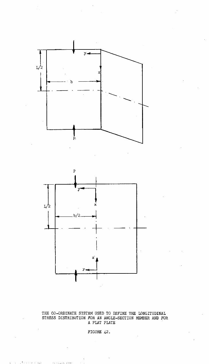
L/2
L/2
b/2,1
THE CO-ORDINATE SYSTEM USED TO DEFINE THE LONGITUDINAL STRESS DISTRIBUTION FOR AN ANGLE-SECTION MEMBER AND FOR
A PLAT PLATE
FIGURE 42.

- 52 -
Stress Distribution Around a Bolt
Before the second mathematical model can be established a
function form for the longitudinal stresses Nx in the neighbour-
hood of the bolt must be obtained. The problem has been simplified
by assuming that the difference between the stress distribution and
the linear bending theory distribution
Nx" = Nx - P/A I Pby/4I pp
(72)
is of the same form for an angle-section member as for a plate. The
functional form for both will be taken as
Nx" = .f(x)(g(y) f Cy + D) . (73)
The coordinate system of the angle is: y measured across the leg of
the angle from the root and x measured in the direction of the load
from the loaded end. Only one half of the member will be considered.
The coordinate system of the plate is y is measured across the plate
from the centre line of the plate and the x :ordinate is the same as
for the angle. See fig. 42. The problem has been considered both
experimentally and numerically.
Only one model was tested experimentally. This was a
1" 4" y 8"x — flat, perspex plate. The load was applied from the
free edge through a bolt. The u and v displacements in the plane
of the leg of the-:anglehaVe:.been,measuredueirig the cross-diffraction
grating method. Also local strain measurements were made using light,
Huggenberger mechanical strain gauges with 1" gauge length to check
the results. Numerically, the problem was examined by a finite
element technique. The basic ideas of the finite element method are
1 discussed by Zienkiewicz. The digital computer programme used was
developed at the University of Tasmania by E. Middleton.
Although only one.model Was tested in the laboratory the effect
of changing the ratio of the length and width of the plate was invest-
igated numerically. The results are indicated in graph 43. It
appears that, as a first approximation, the distribution of the stresses
is independent of the leg width ratio. The effect of moving the point
Ref. 1 0. C. ZienkieWicz, G. S. IT:Aister: "Stress Analysis; John Wiley and Sons.

1.000 lbs.
it, 2
Note; The stress distribution for an 8" x 18" x 1" rectangular plate is the same as given above
400 to an accuracy of 7%. The area of maximum error is very small, and occurs for tension (negative) stresses.
y ordinate (inch)
X =
THE LONGITUDINAL STRESSES IN AN 8" x 32" x 1" RECTANGULAR PLATE LOADED THROUGH A QUARTER POINT AND AT AN EDGE.
FIGURE 43.

- 53 -
of application of the load away from the free edge was also considered
numerically. The two cases were Calculated. The load was applied
at the free edge and at a point one quarter of the leg width from the
free edge. The results are shown in graph 44. It can be seen that,
although the maximum stress under the load was less, the effect was
very local.
As the functional form for the stresses will be integrated in
considering the overall buckling of the member, its accuracy is not
particularly important. The functional form was obtained by using an
average fit in the y direction and by fitting the distribution of the
stresses along the line through the bolt in the x direction. The
one used in the following discussion is
Nx
(P/A I Pby/4Ipp
) + Pe-x/dt(e-(Y- '1,/0)2
+ C Dy) (74)
where 2b is the width of the plate, t is the thickness and d is
the diameter of the bolt. This form applies only in the region
0 < x < L/2 .
Thus, in the following discussion, only half of the angle-section
member will be considered. The parameters A and B are evaluated
by considering the statical equilibrium of the member. The total
axial force and the bending moment on a given cross-section due to the
second term Nx" are zero.
If a more accurate stress distribution is required, it can be
obtained from the stress distribution under a point load on a semi-
infinite plane. However, a term of the form
Nx f(x)(C Dy)
must also be included, to enable the equilibrium of the statical actions
on the general cross-section. This model has not been included as the
mathematical model which follows is sufficiently complex.
Two differential equations can be arrived at, in the same manner
as for the first mathematical model, by considering the equilibrium of a
part of each leg. The equations are

tt
400
C14*
500
•1-
300
cil
200 lbs.
Note: The analytical expression is a better fit to the stress distribution at x = in in Figure 44 than at x = 11" in Figure 43. The distribution in Figure 44 will be closer to the stress distribution in the angle-section member than that in Figure 43.
y ordinate (ins.)
LONGITUDINAL STRESSES FOR AN 8" x 3e, x in RECTANGULAR PLATE LOADED THROUGH A QUARTER POINT AND 2" FROM AN EDGE
FIGURE 44.

- 54 -
a1
DIp/2t :) 30A x3 - a
1 GJ/20/ \dx + .1 a 1 y2 x dy = 0
= (a l - a2 )(+ T 1 2x/L + C dx)
and
_I a2 DI
p/2t 30/2)x3 - a
2GJ/2 \t, 0A x +f a
2Nx2y
2 p/ x dy 0
(a l - a2 )( - T 1 2x/L - c f 0 dx) . 0
When the expression for the longitudinal stress
(y 2 Nx
P/A Py/ 1-2 Ipp + Pe(e-_b/2) C I Dy)/dt (77)
Is substituted into the differential equations, the equations become
too difficult to solve. An approximate result is obtained by using
an averaging, integration process. Firstly, we rewrite equation (75)
assuming that the longitudinal stresses can be expressed as a product
of a function of x and a function of y • Let Nx
1 be the function
of x and K be the result of the integration with respect to y
Then the first equation becomes
a l DI /2t 3Ø/x3 + GJ/2 rEsA x K N1 x = 1 xi
(T 1 2x/L +IC0 dx)(a l - a2 ) . 0
When the equation is multiplied by a l 44/ x 2 and integrated
twice with respect to x the equation becomes
L/2 (a1 2DIp/2(
‘z,2.0/.6 x 2 ) 2 4. GJ/2( x) 2 K 1 Nxl
' x) 2 )dx - j( 0
L/2 x L/2 . - K i N 'xi / x(
\ o 500 x)
2 dx dx - 2T 1 /i Jr a l (a l - a2 )0dx +
0 0 0 L4,2
\ d + 3/2 Ca 1 (a 1 - a 2 )p2 dx = 0
0
for the given boundary conditions. Similarly the second equation (76)
becomes
L/2 f (a2
0 20/ x 2 ) 2 + G J/2( 0/ • x - 2 'DI p/2( a ) + K2Nx2 ( 0/ti x) 2 )dx -
0
L/2 x L/2 i‘ 'A \ 2 - J fK 2 ON / x( OP/0 x) dx dx + 2T 1 /L f a l (a l - a2 )0dx - x2 00
L/2 \ - 3/2 Ca l (a l - a2 )p dx = 0 .
0
If these two equations are added, the sum, which will be referred to as
the "averaging integral", is
(75)
(76)

- 55 -
L/2 (a„:" 4- a 2 )DI /2t( 2Ø/x2)2
GJ/201 90 )02) 2 p
0 ' L/2 x
+ (a 2K N ' + a22K2Nx2
)( x) 2dx - f f (a 1 2K 1 1 Nxl x + 1 1 x1 00 L/2 L/2
cl \ + a22K2x2y/b x)(b 0/
r 2ibx) 2dxdx - (2T'/L Odx - 3/2C W dx)4
0 0
(a 1 2 - 2a 1 a2 a22) = 0
The averaging integral can be treated in the same way as an energy
expression and the same conditions apply, namely
u = 0 and u/ . a1 = b u/4) a2 = 0 • (76)
Also, as the derivative of the differential equations are self adjoint
and positive definite, the value of the critical load obtained by apply-
ing the averaging integral to an approximate shape will be an upper
bounA on the true eigenvalue of the simultaneous, linear, differential
equations. The same conditions apply to both the "averaging integral"
and the energy expression, as both are specific applications of the
least square method of obtaining approximate solutions to differential
equations.1 The energy expression for this problem gives the bound to
a mathematical model which is inherently more accurate than the math-
ematical model considered. Thefirst part of the "averaging integral"
is identical to te equivalent terms in the energy expression for a
plate.
As an example, the first mathematical model will be solved
using the "averaging integral" in conjunction with the functional form
0 = cos 21rx/h + 1 (77)
The conditions for the "averaging integral" to be a minimum are
u/1 a1 = a1 (DI p (21T/L) 4L/8t + GJ(27r/L) 2/8 - PI p(21r/L) 2L/4A _
-4;125 (21r/L) 2/64I pp ) - (a l - a2)0CL/4 = 0,
bu/ba2 a2 (DIp (211r/L) 4L/8t + GJ(27/L) 2/8 - Pl p (21r/L) 2L/4A +
+ LP0(2 1r/L) 2/64Ipp) + (a l - a2 )0CL/4 = 0 •
Ref. 1 Applied Mech. Review Vol.19, No.9, Sept. 1966, "The Method of Weighted Residuals", B.A. Finlayson and L.E. Scriven.

- 56 -
The two equations are identical to the equations of statical equilibrium
obtained previously.
For the second model, the solution to the differential equation
is not known and an approximate shape which satisfies the boundary
conditions will be used,
cos 27r/L + 1 .
Also the term
L/2 x - (a 2K N 1 1 1 x1 x a2 2K 2 Nx2 1 / x)( r" x)2dx 00
will be neglected. For the problem considered, this term is always of
the same sign as the other terms involving the longitudinal stresses
Nx and hence the approximate solution is an upper bound on the solution
of the "averaging integral", and hence to the eigen value of the diff-
erential equations.
The values of the parameters C and D in the expression for
the longitudinal stresses can be evaluated by considering the equations
of axial force equilibrium and moment equilibrium. An approximate
expression is
/2) .2 / (y-b/ pt/A 7 Ptby/4I + Pe-x ke- FT/A 3irby/4I )/dt . (78)
PP PP
The term
L/2 b f N y2 ( 0,/ 30 2 _y dx d
J x 0 0
of the averaging integral consists of two parts
L/2 b 0 f f (y'Pt/A Ptby3/4I )( )90 x) 2 dy dx
PP 00
L/2 b / .2 + y
2Pe-x (e-(-b/2) -11/A 7 ,Firby/4I )() x) 2/dt dy dx .
00 PP
The second part involves the stresses around the bolt. The double
integral can be considered as the product of the two integrals
L/2 Jr e-x ein2 (21ex/L)dx = - 8(e-L - 1)7 /(1611'2 + (L/2) 2 )
. 0
=f 81T2/(1613 2 .-f (1/2) 2 )
and
y2e-(y - b/ 2)2 dy
2 + b 2 /4 . 0
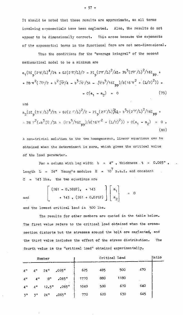
- 57 -
It should be noted that these results are approximate, as all terms
involving exponentials have been neglected. Also, the results do not
appear to be dimensionally correct. This arose because the exponents
of the exponential terms in the functional form are not non-dimensional.
Thus the conditions for the "average integral" of the second
mathematical model to be a minimum are
a1 (DI p (2111L) 4/2t + GJ(211-/L)/2 - PI (217r/L) 2/Az- pb 5 (2m- /L) 2/161 + PP ,
+ P8 2 (/2 + b 2 /4 - b 3 /3A - 174: b 5/16I )/d(16 11' 2 + (L/2) 2 )) - PP
- C(8. 1 - a2) . 0 (79)
and
a 2 (DI p(24(
/L) 4/2t + GJ(2 qL) 2/2 - PI(2M-/L),A2+ OP(21171,) 2/161 +
P PP _, / - 2 / / 2\\ + P8 2 k-b 3 TT;73A + rii- b /5/161 )/d(161 + 'L/2) . )) + C(al - a2 ) = 0 .
PP (ao)
A non-trivial solution to the two homogeneous, linear equations can be
obtained when the determinant is zero, which gives the critical value
of the loan parameter.
For a column with leg width b = 4" , thickness .t = 0.065" ,
length L . 24" Young's modulus E . 107 p.s.i. and constant
C = 143 lbs. the two equations are
(261 - 0.369P), + 143 al l =0
and + 143 , (261 + 0.015P)
and the lowest critical load is. 500 lbs.
The results for other members are quoted in the table below.
The first value refers to the critical load obtained when the cross-
section distorts but the stresses around the bolt are neglected, and
the third value includes the effect of the stress distribution. The
fourth value is the "critical load" obtained experimentally.
Critical Load
4" 4" 24" .065" 625 485 500 470
4" 4" 8" .065" 1770 880 1180
4" 4" 12.5" .065" 1040 580 670 640
3" 3" 24" .065" 770 620 630 645
Member Ratio

-58-
As is to be expected, the effect of the stress distribution around the
bolts is negligible for long members. The ratio of the deflections of
the two flanges does not change appreciably with the inclusion of the
secondary stresses. The largest change was for the 4" x 4"
0.065" member, in which case the change was an increase of ten
percent.
As for previous models tested, some of the members stiffened
for loads greater than the "critical load". The member with a leg width
of four inches and length of twenty four inches carried en ultimate load
of 720 pounds, compared with a critical load of 470 pounds. On the
other hand, the ultimate load and the critical load of the member with
the leg width of three inches were identical. For the second member,
the material yielded before any significant longitudinal strains due to
the twisting of the section were produced.
The angle-section members tested were all bent from thin alum-
inium sheet, and consequently the roots of the angle-section members were
weak. Extruded angle-section members quite often have a heavy fillet
at the root of the section. For these members, the author does not
think that the 'Mathematical model developed in this section will apply.
One would expect that for these members the angle contained between the
two legs of the member would remain constant, and that there would be an
appreciable amount of bowing of the legs. If this is the case, a math-
ematical model could be developed using a functional form of the type,
w l = (a 1 y2 + by)0(x) and w2 = (a2y2 + by)0(x) .
The problem could also be treated by the usual method of considering each
leg as a,plate, and applying compatibility of geometry and statical
actions at the root. This method, used often in published work, will
be discussed in the conclusions at the end of this thesis.
TORSIONAL-FLEXURAL BUCKLING
One of the basic assumptions of the previous part of this chapter
was that the line of shear centres remained straight and that the sect-
ion rotated in an undeformed state about the Shear centre. For long
members, the foregoing assumption is no longer justified because the
member bends. In this chapter on buckling it has been shown how Euler
developed a mathematical model which took into account the possibility

critic
al lo
ad
FIGURE 45
20
15
1 Torsional instability curve 2 Flexural instability curve 3 Torsional-flexural instability
10 1 2 curve
3
20 4 60 80 l0
length L (in)
THE VARIATION OF THE CRITICAL LOAD OF THE TORSIONAL-FLEXURAL MODE OF A 4" x 4" x 1/8" ALUMINIUM, ANGLE-SECTION COLUMN
FIGURE 46.

- 59 -
of the members buckling by bending. In the following section the
interaction of the torsional mode and the flexural mode will be consid-
ered. This exercise has been carried out before by various people,
2 including Bleich, Timoshenko
2and Goodier 3 but in this thesis the
equations of statics will be established directly by the same method
as that used in th models developed previously.
The notation introduced before will be maintained except that
the deflections of the shear centre not the centroid in the directions
of the two principal axes will be denoted by p and q • Thus as the
polar-coordinate of the centroid is b/2 the displacements of the
centroid are q + 0 b/277 and p • Thus the total moments about the
two principal axes of the cross section are
= P(q Øb/2 r2)
( 8 1 ) and
MQ = Pp ,
which, in conjunction with the load deformation relationship, gives the
two differential equations
El 2,:01 x2 = - P(q + Øb/2 72) PP
1 2p/ x2 = pp and EI
The longitudinal stresses produced by bending of the member are
Nx
P/A + Pp(y - b/2)/ [7 I QQ P(q + 4/2 1-2)y/ ,11 I PP
The St. Venant shear stresses are
GJ 2w/ y = GJØAx
and the plate bending, shear stresses Qx are
- r)30/ x3 + Nxy 95/1 x - Nxy0
The equation of torque equilibrium on a section, with x constant, using
the values quoted above, becomes
Ref. 1 F. Bleich: "Buckling Strength of Metal Structures", McGraw-Hill Book Co. Inc.
Ref. 2 S. P. Timoshenko & J. M. Gere: "Theory of Elastic Stability", McGraw-Hill Book Co. Inc.
Ref. 3 J. N. Goodier: "Torsional and Flexural Buckling of Bars of Thin Walled Open Sections Under Compressive and Bending Loads", A.S. M.E., Trans. 1942.

- 60 -
T =0 = (DI p/t)03A x 3 - GJAILVe,x -
11 _ 0 (pt/A)(( x - P/2) x)/V + x)y dy -
(pt/A)(( x + x)/ r2 + Y 19JA x)y dy -
-f (Ptp(y - b/2)/ r-2IQQ )(( q/ x - /e )/r2 + y x)y ay - o
- (PtP/y - b/2)/ DIQQ )((b x + x)/ + y c)0/ ex)y dy -
(Pt(q + b0/2 )( ( q/6 x - x)/ y), 0/) x)y dy - PP 0
- (pt(q + b0/2 i )((. q/ 2>x + x)/ Y )0/6x)y dy (82) PP
which simplifies to
DI /t )30/3c 3 + (PI /A - Gc3-) 0/6x + Ptb 2/ 2,q/x +
+ Ppt/6i
QQ q/2) x + 1/ D )10/6x) - Ptb4(q + b0/2 r.2)/4I P/e‘x = 0. PP
A set of solutions to the three simultaneous differential
equations (81e), (B1b) and (82) in 0 p and q for simply supported
boundary conditions is
0 = 00 sin nirx/I,
p = po sin nlrx/I)
and ci = qo sin nTrx/L
provided the conditions
and
p000 = 0 ,
00Ptb 2/A + PtI p/A00 - DI p (Tr/L) 2/t00 - GJO0 = 0
/ . EIppq0 ( 1r/L) 2 = p(q + b0/2 T5) 0
/ EIQQp0o(/L) = Pp 0
are fulfilled.
The conditions indicate that there are two independent modes of
failure, either p = coo , 0 = 0 and q = 0 , which is the case
of pure flexural buckling about the minor axis, of q = ago and 0=0. p = 0 , which is a mode in which there is an interaction between
bending about the major axis and torsion. The critical load for the
first type of failure is Euler's buckling load.
(83)
(84)
(85)
(86)
(87)
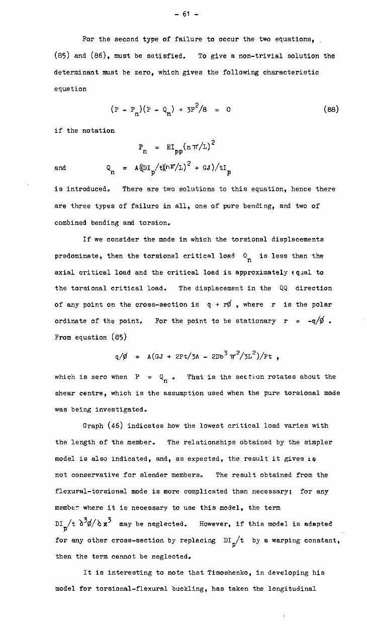
- 61 -
For the second type of failure to occur the two equations,
(85) and (86), must be satisfied. To give a non-trivial solution the
determinant must be zero, which gives the following characteristic
equation
(P - Pn)(P - Qn ) 3P2/8 = 0
(88)
if the notation
Pn
= El (n -rr/L) PP 2
and
Qn = op' /t)(nr/L) 2 + GJ)/tI
/ .
is introduced. There are two solutions to this equation, hence there
are three types of failure in all, one of pure bending, and two of
combined bending and torsion.
If we consider the mode in which the torsional displacements
predominate, then the torsional critical load O n is less than the
axial critical load and the critical load is approximately Equal to
the torsional critical load. The displacement in the QQ direction
of any point on the cross-section is q + r0 , where r is the polar
ordinate of the point. For the point to be stationary r =
From equation (85)
q/0 = A(GJ + 2Pt/3A 2Db 3 Tr2/32)/Pt 9
which is zero when P = Q n • That is the section rotates about the
shear centre, which is the assumption used when the pure torsional mode
was being investigated.
Graph (46) indicates how the lowest critical load varies with
the length of the member. The relationships obtained by the simpler
model is also indicated, and, as expected, the result it gives is
not conservative for slender members. The result obtained from the
flexural-torsional mode is more complicated than necessary; for any
member where it is necessary to use this model, the term
DI /t '?3Ø/x3 may be neglected. However, if this model is adapted
for any other cross-section by replacing DI p/t by a warping constant,
then the term cannot be neglected.
It is interesting to note that Timoshenko, in developing his
model for torsional-flexural buckling, has taken the longitudinal

- 62 -.
stresses as constant, when he considers the torque equilibrium. In
the previous calculations the variation in the stresses due to bending
has been included and this has produced the equation,
p0Ø0 =0,
which is a redundant equation.
Eccentric Loading
Both Timoshenko and Goodier have produced models for the buck-
ling of members experiencing axial loads and end moments. Although
the approaches adopted differ, the assumptions are the same, and so
are the resulting differential equations. Both assume that the long-
itudinal stresses depend only upon the applied loads. Goodier gives
the three equations of statics as
EI QQ ) 213/ x 2 + Pp + MRS = - MQ
EI 2ci/e. x 2 + Pq + (M + Pb/2 5)0 = - M'
(90) PP P
and DI /t )330/)3 x3 - (GJ - Mp7b/4 2 - PI /A) 1?0/b x2 +
m .2 coo x2 /Pb
/ k/ 2 17 M) 1 2 10 x2 . 0 . (91)
Both Timoshenko and Goodier assume that the graphs of the
deformations p, q and 0 against the loads are asymptotic to a
given load condition. At a load near the critical load the equations
of statics, stated above, are satisfied. If pl, ql and 0 1 now
denote the change in deformations from this state, the new equations
of statical equilibrium have zeroes on the right hand side, as the
change in the loads is negligible. In making this assumption the
problem has been forced into an eigen value problem. Thus while the
load-deformation relationships obtained will be erroneous, the critical
loading conditions obtained should approximate to the asymptote of the
real relationship.
The end moments of the models tested have been applied by means
of an eccentric load, thus, if the moments are M = - Pe and
MQ
= -Q
the critical conditions become
/ . EI QQ (Ir/L)
2 p0
- Pp0 + PeQ00 . 0
(89)

- 63-
/ EI
pp(Tr/L)a q
0 - Pq
0 p(b/2 — e)Ø
0 = 0
and DI (V/L) 30O/t + (GJ - 7M b/4 T-2 - PI /A)(Tr/1) 2
+ (Pb/2 — Pep)p0(TrA) 2 = 0 .
It should be noted that when the load is eccentric about both axes all
three types of instability are combinations of the torsional modes and
the flexural modes about both axes. The three critical loads are
the solutions to the cubic, characteristic equation obtained from the
determinant of the above equations.
For the case where eQ
0 , the characteristic equation is
(Pn - P)(QnI0/A - P(I0/A - 7bep/4 17)) - P(b/2 ep ) 2 = 0 .
(92)
The critical load is infinity when the eccentricity is approximately
0.38b/ TT, which compares well with b/3 F for the simpler model.
When e = 0 the characteristic equation condenses to
(p _ pn l)((p - Qn)(P - Pn ) - P2ep2A/I0 ) + Pb 2A(P - Pn)/8I0 = 0
which indicates that the lowest critical load is not independent of
bending about the major axis, as obtained from the simpler model.
Pn' is the other flexural critical load. However, if the character-
istic equation is expressed in the form
= Qn
- PA/I0 (ep2/(P
n1 /P - 1) + b 2/8(Pn/P - 1)) 9
It follows that as the ratios P/Pn
1 and P/Pn
tend to zero, as
would be the case for a torsionally weak member, the critical load
tends to the critical load for the torsional mode of a column loaded
through the centroid.
This section of the thesis has extended the mathematical model
to make it more applicable to members met frequently in engineering
practice. It has also shown that the simpler model is the limiting
case of the more complex model.
SUMMARY
In this chapter has been established mathematical models to
describe the behaviour of the columns tested by the author. Although
each mathematical model has been discussed at the end of each major
section of the chapter, it is thought worthwhile to briefly summarize

- 64 -
the chapter.
Mathematical models have been developed to describe the buck-
ling mode of short columns loaded with en axial load, with en end
moment about the minor axis, or an end torque. The second mathematical
model is recommended as the most practical model.
The next section of the chapter deals with columns loaded through
one leg. While the mathematical models developed are really only
relevant to the type of member tested, that is angle-cross-sections
with little or no fillets, the mathematical models indicate two things.
The assumption that the cross-section does not distort when the column
is loaded eccentrically about the major axis is a non conservative
estimate. The second point is the actual manner in which the load is
applied, or the longitudinal stress distribution near the ends, has no
important effect on the overall buckling mode and load of the member.
However, end connections are important as far as regards secondary
effects, such as local buckling due to high stress concentrations or
weakness in the metal due to heating.
The third section develops a mathematical model describing the
flexural-torsional buckling modes of long members. The mathematical
model is basically the same as the ones developed by Timoshenko,
Bleich and Goodier.
All the mathematical models use the basic functional form of
straight lines across the leg of the angle remain straight during
buckling, and all the problems are attacked by the same approach.

the root of the angle-section member
loaded end
FIGURE 47
deformations
AB - small, elastic deformations BC - large, elastic deformations CD - elasto7plastic deformations DE - plastic unloading with a control on the deformation DE' - plastic colli4pse
TYPICAL LOAD-END ROTATION RELATIONSHIP FOR A CENTILEVER.
FIGURE 48.
LIGTENBERG FRINGES (ew/6x) for A POINT LOADED CANTILEVER
FIGURE 49

STABILITY OF ANGLE-SECTION BEAMS
This chapter deals with the stability of angle-section beams
in bending. The majority of the experimental work associated with
this chapter was done on cantilevers. However, the ideas obtained
from the results and the mathematical models developed are used to
discuss the general stability of angle-section beams and to predict
the behaviour in a number of cases. Some simply supported, centrally
loaded beams have also been tested. The chapter is limited to the
case of bending about the minor axis, although, following the work
done on columns with eccentric loads, the effect of bending about the
major axis will be discussed.
The members tested failed by local instability, but the failure
of members by overall lateral instability is also discussed.
STABILITY OF ANGLE-SECTION CANTILEVERS
To examine the stability of angle-section beams in bending,
several cantilevers were tested. When a cantilever was loaded so
that compressive stresses were produced at the root of the angle the
instability was due to plastic bending deformations and it was found
that the failure load could be estimated using the common,fully
plastic analysis method for beams1 When the outstanding legs of the
angle member were in compression, the member was unstable in the
elastic range. For the members tested the instability mode was one
of pure torsion, the deflections caused by twisting being much larger
than those caused by the bending of the member. The loads at which .
the members failed were considerably smaller than those calculated
2 from the lateral buckling model of Timoshenko. The mode obtained was
due to local buckling of the legs of the angle. The main body of the
chapter will be devoted to establishing a mathematical model describ-
ing the local buckling mode. The relevance of the lateral buckling
mode will be considered at the end of the chapter.
A typical graph of load against total rotation is shown in fig.
48. The graph can be divided into four sections. In section AB the
Ref. 1 J. Baker, M. R. Horne, J. Heyman: "The Steel Skeleton", Vol. Cambridge University Press.
Ref. 2 S. P. Timoshenko: "Theory of Elastic Stability".

The loading of an angle-section cantilever.
FIG. 50
The plastic deformations of a cantilever. The member on the left has been allowed to collapse without any control on the deformations.
FIG. 51

- 66 -
rotations are small and the section rotates in an un-deformed state.
In section BC the rotations are large but elastic. In section DE
most of the deformation takes place in a relatively short length and
the cross section experiences plastic distortion. The plastic mode
is shown in fig. 51. An isosceles triangle is seen in both legs.
The total rotation is approximately 30 0 . This mode is independent
of the leg width and the length. Section CD is an intermediate state
between the elastic large deformation mode and the fully plastic
"triangular" mods.
Apparatus
All the angle section cantilevers were bent from 0.050 inch
aluminium sheet. For all the members the ratio of the leg-width b
to the thickness t far exceeded the allowable structural design
code value 16 . Models were tested with various leg-widths b and
overall lengths L
To produce a "built-in" end, each leg of the cantilever was
clamped between a flat plate and a side of a vee block as shown in
fig. 47. The plates were held securely with four quarter inch diam-
eter bolts. The mounting was such that zero twist )91/x occurr-
ed at the "built-in" end of the cantilever. The models were loaded
using dead weights. However, in the plastic range, the deflections
were controlled so that measurements could be made while the member
unloaded plastically (that is on the downwards sloping part DE of the
load-deflection curve).
The loaded shape of a cantilever WPS measured using the Lig-
tenberg reflective method. When the Ligtenberg apparatus was used
the model was mounted so that one leg was vertical. This necessitated
loading the model through a pulley system. Strains at required places
on the legs were measured using mechanical,Huggenburger strain gauges.
Point rotation measurements were taken using a light source and a
small mirror mounted on the model.
Small Deflection, Elastic Mathematical Model
First, the discussion of the problem will be limited to one
involving small rotations. The mathematical model will attempt to

- 67 -
describe section AB of the load-deformation graph. The elastic,
small deflection plate theory is relevant, and the results derived
in appendix A, will be employed. The Ligtenperg moire fringes show
that all sections rotated without deformation of the cross-section.
They also show that for some members only part of the member
twisted. The fraction of the cantilever which deformed depended
upon the ratio of the leg width to the length. This fraction
decreased as the ratio decreased.
To establish the mathematical model the following co-ord-
inate system is set up. The co-ordinate is measured along the
cantilever from the free end and the y co-ordinate is measured across
the leg from the root of the angle. The deformations out of the
plane of the leg are denoted by w and the rotations, that is
y , by 0 (see fig. 47). A basis for the mathematical
model will be w = y0(x) , where 0(x) is a function of x only.
The longitudinal stresses Nx will be linear in y and unaffected
by the deformations. Initially the unloaded member will be taken
to be straight. The expression for the shear stresses, O x derived
in Appendix A under these conditions becomes
Qx = - -.1) ) 2.w/e y - x
- M y . xy
From the moment equilibrium and the axial force equilibrium on a
section, x constant, the longitudinal stresses are
Nx = Wx(y - b/2)/Icx2 17 9 (93)
where W is the point load applied at the end of the cantilever.
The torque equilibrium about the x-axis produces the differential
equation,
(2b 3D/3) )30/ x3 + (b4 tWx/6 f.-Nc2 ) 0/ x — GJ reC/b x = 0 (94)
which can be simplified to
1) 30/2) + dx ord - aØ/x = 0 (95)
by substituting d = Wbt/42DI QC2 and a = 3GJ/2b 3D .
The stability of the differential equation can be investigated

68
by examining the adjoint properties of the equation, as explained in
the chapter on buckling. The differential equation is of the form
2Ø/2 + x A wo ?C 0= 0
If 0r and 0s are any two solutions of the differential equation
which also satisfy the boundary conditions; 0 = 0 at x = 0
and x = L then the integrals
csr ( VI x2 + )sos ) - 08 ( 29S1 x 2 + 0r )dx
and 0 45rris x°s9Cr dx
are zero if the equation is self adjoint. The second integral is
zero and the first simplifies to
Jo. ( 0r 20s/ x2 os 20r/ x2) dx 9
which on integration by parts leads to
0r '95s/ x jLLL PirA x 4s/ x)( 01A ")
4 0.3(0 0 sd) x) dx
Under the boundary conditions the second integral takes the value
zero. Hence the differential equation is self adjoint and there are
an infinite number of orthogonal, eigen functions and eigen values
(P 0 ) That is, the mathematical model predicts that the rotation r r
is zero for all loads except the eigen values, at which loads the
rotation is infinite.
When the member has an initial crookedness 0 the differ-.
ential equation can be expressed in the form
2 (0 - 00 )/ex 2 +00 ) + xwX0 = 0,
From the self—adjoint properties of the differential equation of the
initially straight member it follows that the initial shape can be
expressed as a unique sum of the orthogonal eigen functions,
CO 00 =
r E. A Or =1 r
and the shape 0 for any initially crooked member is

-69-
co A r d = 1 - W/W )ur
r=1 r
Physically, this means that the rotation tends to infinity as the load
approaches the lowest eigen value.
The differential equation (95) can be solved directly. An
expression for the lowest critical load, or eigen value, will now be
obtained. The solution of the equation is
90 x = A l tdx -- a J 1 /3 (2(dx - a) 3/2/3d) + A 2 57:77J_1 /3
(2(dx - a) 3/2/3c6 (96)
where A1 and A 2 are constants. It can be seen that for small x
this expression is immaginary as dx - a is negative. If
- 1) - a = 0 , then we define 1 as the effective length over
which the member deforms. For x = L - 1 it is assumed that
x = 0 • From the moire fringe photographs (fig. 49) the
boundary conditionsara0Ax = 0 at x = L and x = L - 1 .
The second condition gives A 2 = 0 as J.43 (0) = a), and the
first condition gives
2(d1, - 10 3/2/3d = 2.9 , (97)
as 2.9 is the first zero of the Bessell function of the one third
order. This implicit equation can be solved for the critical load.
The other eigen values can be obtained by replacing 2.9 by the approp-
riate zero of the Bessell function.
As an example consider a cantilever with b = 2" ,
= 1/20" 9 L = 10.25" 9 E = 107 and‘ = 0.3 • Then
a = 3GJ/2bD = 6(1 -70)/b2
= 1,05
and d = 3W1/2b 2D = 0.00464 .
The implicit equation can be solved by trial and error to give
W it = 41 pounds. The length of the member which is distorted is cr
1 = L - a/d = 10.25 - 1.05/0000464 = 4.5" .
These values compare well with the experimental values of 40
pounds and 4075" • The shape predicted mathematically is compared
graphically with the one obtained experimentally on graph 52. The

r0
U)
4 experimental point --mathematical shape
i)whoc = (2(dx-a)
6 8
X •
ratio of lo
ads
COMPARISON OF EXPERIMENTAL AND MATHEMATICAL SHAPE OF L. 2" x 2" x 1/20" 1ALUMINIUM CANTILEVER, LENGTH L = 10.25"
FIGURES
leg width - length ratio L/b
NUMERICAL DETERMINATION OF APPROXIMATE EXPRESSION FOR THE CRITICAL LATERAL LOAD
FIGURE 53.

- 70 -
agreement between the two shapes is acceptable although the following
table indicates the agreement is not always as good.
4 •Z +3 0
1-q
o .p 0
tiprd.ri CD -r1
r-1
0 m 0 04-1 cu
+-P
-P ---, .ri m $.4 .0 Or-1
-e •-4 f..4 0
P4 ■,„„.
..4 I
-P .0 0 -P CD 40 4-1 0 0 4-1 W
-1-1
ncl f-I CD
g tO 0 0 QQ)
-
12.5 3 0.05 60 4 36.5 0.50 6.2 7.4
10.25 2 0.05 40 5 41 0.54 4.70 4.75
18 2 0.05 40 9 19 0.66 6.1 6.9
41.5 2 0.05 .40 20.5 6.8 0.80
60 4 0.25 16 15 62.5 0.77
30 4 0.25 16 7.5 1,400 0.63
6 0.8 0.037 22 7.5 110 0.63
From inspection of the implicit equation (97) it is obvious
that
W' = 2 1-"i( )D/L
is a lower bound to the critical load. The ratio of the lower bound
to the critical load has been calculated for various-sections. The
ratios appear in the above table. It has been fo land that, as a
first approximation, the ratio is independent of the leg-width to
thickness ratio b/t , but varies with the length to leg-width ratio
L/b . The ratio is plotted against L/b on graph (53) for various
b/t . The algebraic expression for the relationship is
wcrit L/b W' L/b + 4.71
or crit • w'(1 + 4.7bYL
This leads to an approximate expression for the critical load.
Wcrit = 2 E(1 )D (1 + 4.7b/L)/L .
(98 )
Although the approximate formula was derived empirically, a
numerical justification can be made. If the load is found by an
iterative process it becomes
VV= a/dL,
then NV . a(1 • 1.65 (b/L) 2/3 )/dL s
and then V/ . a(1 + 1,065 (b/L) 2/3 (1 + 1.65 (b/L)2/3)2/3)/dL ,
or in simple terms P = (a/dL) (a function of .b/L)
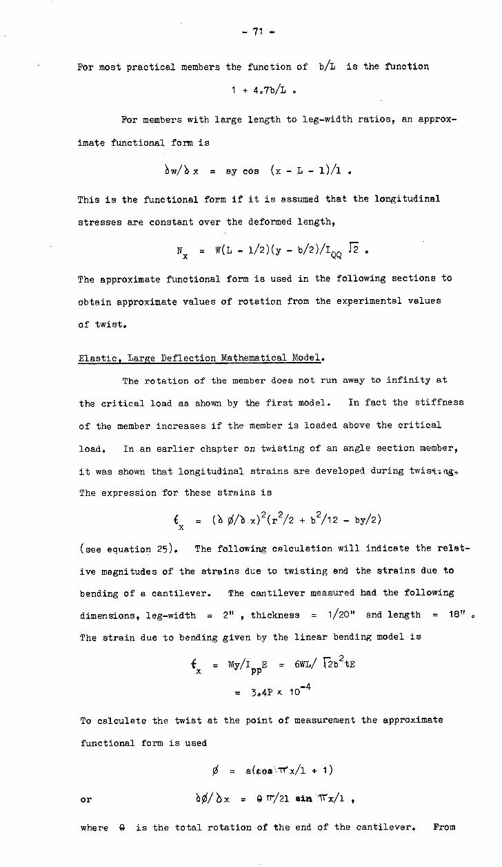
-71 -
For most practical members the function of b/L is the function
1 + 4.7b/L
For members with large length to leg-width ratios, an approx-
imate functional form is
= ay cos (x - L - 1)/1 .
This is the functional form if it is assumed that the longitudinal
stresses are constant over the deformed length,
Nx = W(L - 1/2)(y - b/2)/I QQ
The approximate functional form is used in the following sections to
obtain approximate values of rotation from the experimental values
of twist.
Elastic, Large Deflection Mathematical Model.
The rotation of the member does not run away to infinity at
the critical load as shown by the first model. In fact the stiffness
of the member increases if the member is loaded above the critical
load. In an earlier chapter on twisting of an angle section member,
it was shown that longitudinal strains are developed during twisttn.
The expression for these strains is
(x =( Ø/ x) 2 (r2/2 + b2/12 - by/2)
(see equation 25). The following calculation will indicate the relat-
ive magnitudes of the strains due to twisting and the strains due to
bending of a cantilever. The cantilever measured had the following
dimensions, leg-width = 2" 9 thickness = 1/20" and length = 18"
The strain due to bending given by the linear bending model is
= my/I ppE = 6wL/ 51) 2tE
= 304p x 10-4
To calculate the twist at the point of measurement the approximate
functional form is used
0 = a(cos\Trx/1 + 1)
or bebx = QIr/2l Sin 'Vx/1
where G is the total rotation of the end of the cantilever. From

20
suspect shift in values, this would explain the disagreement
15
strains based on the linear bending model
10 9 measured strains 0 calculated strains based on Fig. 54
-0005 +.005 .010 .015 • I •
20
late
ral lo
ad
15
5 •
20 15 20 •
25
total end rotation 4 (degrees)
LOAD -END ROTATION GRAPH FOR A 2" x 2" x 20" ALUMINIUM CANTILEVER,18" LONGr
FIGURE 54.
strain ('
LOAD -STRAIN GRAPH FOR TWO POINTS ON A 2" x 2" X 1/20" ALUMINIUM CANTILEVER, 18" LONG
FIGURE 55.

- 72 -
the load-rotation graph for the values of the end rotation for the
loads 19, 21 and 21.5 Pounds, are 10 0 , 160 and 190 respectively.
See graph 54.
For P . 21 pounds, = 160 = 0.28 rads, therefore
= (0.28/2)(9117) sin (21T/7) = 0.049 , therefore
tx
1 = ( 0 .049) 2/3 = 0.0008 • At a load of 21.5 pounds the max-
imum strain is 0.0015 and at 19 pounds it is 0.0003.
The experimental and calculated strains are compared in graph
55. As was to be expected, the twisting strains are of the same
order as the bending strain near the critical load. Consequently
the small deflection model breaks down. It should be noted that the
load at which the twisting strains become important depends upon the
initial crookedness of the member.
If the twisting strains are taken into account, the moment
about the shear centre of the w-component of the longitudinal stresses
must be modified. The integral becomes
0 Nxy x dy = (Wxb4/6 r2 IQQ ) x + Eb5t( 0/e x) 3/180
The approximation for the curvature Kx = ) 2‘0 x
2 , is still
applicable even for the largest twist measured, which is of the order
of 0.05 rads. per inch. When this integral is included the differ-
ential equation describing an initially straight member becomes
(DI /t))) 30ni x3 +kNA?b4t/6 p IQQ
- G,T)):) 9C/. x + Eb 5t( x) 3/180 . 0
(99)
No solution has been found for this equation. However, for the members
with large leg width-thickness L/b ratio an approximate maiel could
be established, if it is assumed that the longitudinal bending
stresses do not vary within the deformed length of the member. In
this case, the large deflection model for a column could be used to
obtain an approiimate load deformation relationship.
Fully Plastic Mathematical Model
As the deformations become large, the material yields and
plastic effects become pronounced. The cross section distorts and
finally the member collapses, or unloads if it is loaded so that the
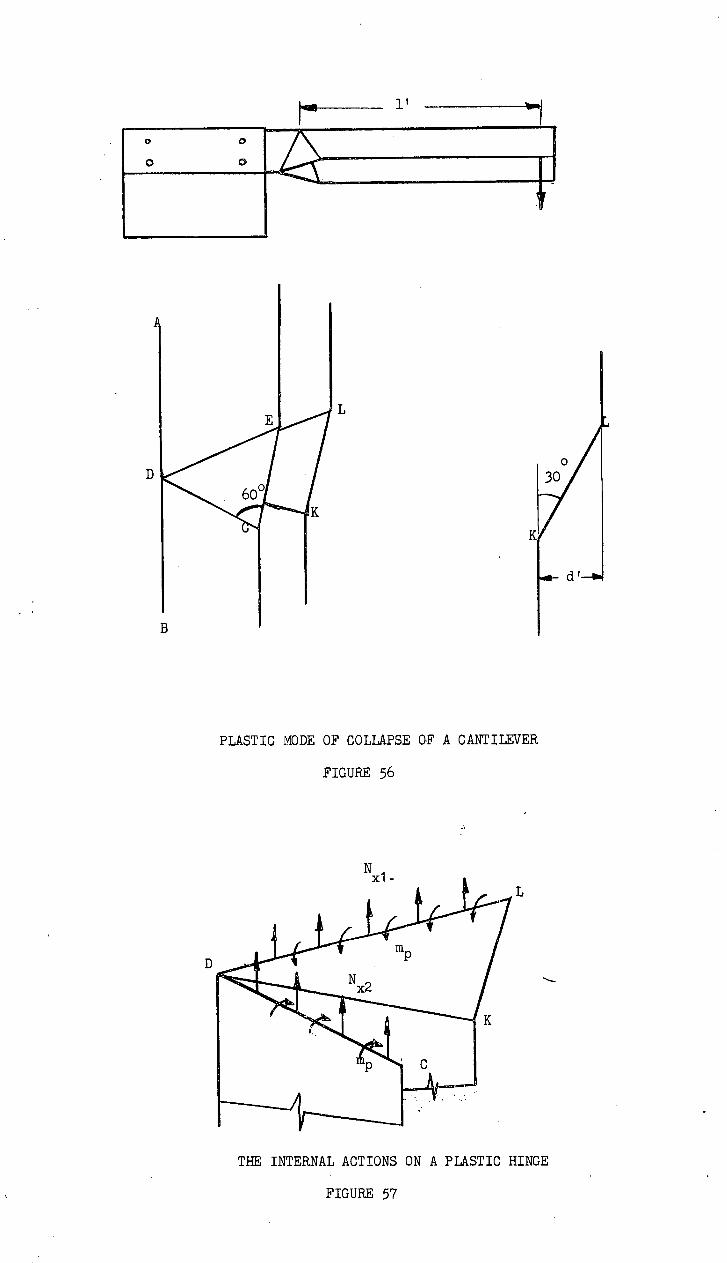
THE INTERNAL ACTIONS ON A PLASTIC HINGE
PLASTIC MODE OF COLLAPSE OF A CANTILEVER

- 73 -
deflections are controlled. The fully plastic mode of failure by
buckling is shown in figs. (56) and (57). It is interesting to note
that the apices of the triangles form at the plane of maximum twist.
Here, the maximum moment is at 450 to the axis. In practice the
line of plastic moment is formed at sixty degrees. The difference
in the angle is probably due to changes both in the twist and the
moment over the deformed length.
A mathematical model was developed for this mode, as it was
hoped to produce an upper bound on the load the member can carry.
This did not prove, successful, as, in most cases, the fully plastic
mode was formed after the member partially unloaded. The functional
form for the mathematical model as shown in fig. 56. Both triangles
DEC and DLK are isosceles triangles and the lines EC and LK are
both at thirty degrees to DA • The line ADB remained straight
when the mode was first formed. The mode was the same for all the
different members considered.
Using the notation, that Nx1 and Nx2 are the longitudinal
stresses in the two legs on either side of the "plastic hinge", 1 1
is the distance from the load to the apex of the triangle, d is the
maximum displacement and m is the plastic moment per unit length,
the following equilibrium equations are obtained:
The moment equilibrium about the minor axis for the material to the
left of CDK gives
2 f Nip dy = + 4bm cos 60°/cos • (100) 0
The moment equilibrium about the minor axis for the material to the
left of CDL gives
2f Nx1p dy + 2 f Nx2p dy = 2W1' .
0 0
Vertical stress resultant equilibrium gives
)( Nx1 dy = - f Nx2 dy .
0 0
, Now consider moment equilibrium on triangle .DEC , and we obtain
(102)
f Nx1 dy/2b dy + Nx2 dy/2b dy = - 2bm 0
(103)

FLAT PLATE CANTILEVER
FIGURE 58.
111E1131 (a) 1011b Y
NI EWE (b) 14/ktx
_he Ligtenberg fringes predicted by Timoshenko's model of lateral buckling of a cantilever
if//A (d) 6w/ex
The Ligtenberg fringes obtained experimentally
FIGURE 59.

- 74 -
If equations (100), (101), (102) and (103) are combined, and we note
that y = 12p + b/2 , then
d P- W1 1 /4b + d ,P.(1U112 + 2mb )2b = •2bm
( 104)
For a cantilever of length, L = 10.25" , and leg width b = 2"
and plastic moment m = 12 pounds per inch, the expression gives the
load P = 23 pounds, which compares favourably with the measured
value of the load 27 pounds. For a cantilever of length forty-three
inches the estimated load is 4.9 pounds and the measured value is
6.1 pounds.
LATERAL BUCKLING OF A CANTILEVER
As mentioned before, none of the cantilevers tested failed by
lateral buckling. However the members tested would not find general
use in practice. All members should be tested both for local buckling
and lateral buckling.
Lateral Buckling of a Strip
Timoshenkols lateral buckling model1is identical for both an
angle-section cantilever and a flat plate cantilever as for both sect-
ions the primary warping is neglected. A flat plate cantilever was
tested to check the validity of Timoshenko's model (see fig. 58).
Fringes typical of Timoshenko's model are shown in fig. (59)
a and b, while fringes which were obtained are shown in fig. (59) c
and d. Fig. c indicates that the bending deformations are large
compared with the twisting deformations. Fig. d indicates that the
built-in end does not prevent warping of the cross-section to any
extent, in this respect the boundary conditions agree with Timoshenko's
model, which states that the maximum twist is at the built-in end.
Fig. d indicates that the cross section has deformed.
The local buckling of the seCtion is due to the variation of the
strain across the model due to the applied moment. The same type of
local buckling occurred when the author tested a flat plate loaded eccen-
trically as a column. In the case of the column the function form was
Fig. 1 S. P. Timoshenko & Gere: "Theory of Elastic Stability", McGraw-Hill Book Co.

- 75 -
= A(y + B) 2 sinlrx/L
where A and B are parameters, L is the length, y is measured
across the plate and x in the direction of the load. One would
expect the distortion of the cross-section of the cantilever to be more
prominent than that of the column, as no axial load is present.
The local section deformation appears to be a secondary effect
and has no effect on the load capacity of the member. For a
2" A .052" K 9.25" aluminium cantilever with a Young's modulus of
_6 10 x 1. p.s.i., Timoshenko gives the critical load as
crit = 2Ebt 3/2 2(1 +1) ) L2
. 13,6 pounds,
The critical load of 13.6 pounds is obtained from the Southwell plot
on the bending strains.
Timoshenko gives the critical load for an angle cantilever as
4„013Eb 2t 2/3L2 F1-77:1) „ (106)
For the sake of the comparison we shall use the approximate local
buckling load. For the member to fail by lateral buckling, the
following inequality must apply,
4.,013Eb 2t 2/32..17-r--t) 2 M1 - -1))D(1.+ 4.7b/LVL
or b/L < (t/b(1 + 4.7b/L)/4.013 i2(1 +-))
(107)
For most extruded aluminium section the ratio of the leg width to the
thickness is sixteen, the ratio laid down by steel codes. For such
members, lateral buckling will occur if L/b is greater than 104 .
The bending stiffness of the leg of the angle-section member
can be taken into account using Timoshenko's model for the lateral
buckling of cantilever in which warping of the cross-section is
included. Timoshenko gives the buckling load as
P = Eb 2t2/32 J 1 4. 1) crit
and quotes values of X for value ratios of L2GJt/DI or
6(1 - -1) )(L/b) 2 As the ratio tends to infinity, X tends to
4.013 • For large ratios Timoshenko gives the approximate relation-
ship

the shape of the free edge of the loaded member
FIGURE 6
ONE OF THE SETS OF SUPPORTS USED FOR TESTING SIMPLY SUPPORTED BEAMS
FIGURE 62
wA x = 0
the shape of the free edge of the loaded member
THE LIGTENBERG FRINGES OF )1,,,r/ex OF ONE LEG OF AN ANGLE-SECTION BEAM FOR THE TWO POSSIBLE MODES
FIGURE 64

- 76 -
= 4.0 1 3/( 1 - b/L i6(1 - ))
which for practical applications, equa -s.s 4.013 . For the more detail-
ed model the twist at the built-in end is zero. Thus there must be a
very local change from zero twist to maximum twist in the vicinity of
the built-in end.
It is possible to consider the interaction between the local
buckling mode and the lateral buckling mode. The three equations of
statical equilibrium on a section normal to the axis of the cantilever
are
EIQQ
b2p0) x 2 + Px = 0
El x 2 pxo = 0
PP
and DI /t VO/ x 3 - GJ g5/x + Plx•cA x + P(q i - q) +
+ (P1b4t/6QQ
x = 0 ,
which combine to give
DI /t ;1 4r?fA x4 + (PLb 4t/6QQ
- G,T) 9C/2)3c — P2x20/EI . 0 . pp
This equation must be solved by an approximate method, and as the
equation can not be expressed in a form so that the self adjoint test
can be applied, there would appear to be no available indication of
the relationship between the approximate eigen value and the true
value.
SIMPLY SUPPORTED BEAMS
Central Load
The bending moment diagram for a simply supported, centrally
loaded beam is linear. The boundary conditions for the twist are such
that half the beam can be cbnsidered as a cantilever. The maximum
bending moment for the beam is WL/4 . Thus the differential equation
is
b 3D( )3r/O)x3 )/3 + b4tWx( x)/12 r2 - GJ() ox) = 0 , (108)
or
395/6 x3 + (dx - a) Ø/x =
and the Critical load is
Wcrit 4 5(1 - 1) )D(1 + 9.4b/L)/L . (109)
The notation is for a cantilever and is defined in fig. 62.

A simply supported beam as arranged when the Ligtenberg apparatus is used to measure the shape. The buckling mode is the elastic symmetric mode.
FIG. 60
The plastic deformation of a simply supported, centrally loaded beam.
FIG. 61

- 77 -
A few beams were tested under two sets of conditions. One set
of supports consisted of rollers in vee-blocks as shown in fig. 62.
The alternative set of supports, illustrated in fig. 60, was used in
conjunction with the Ligtenberg apparatus. Some experimental results
obtained by Gregory were also used to extend the available information.
Some of the beams which were tested buckled in the symmetric mode
described above, see Ligtenberg fringes in fig. 63. For this mode
the implicit equation is
2(dL/2 - a) 3/2/3d = 2.9 . (110)
(See equation 97.) Other beams buckled in an antisymmetric mode.
The fringes obtained are shown in fig. 64. The boundary conditions
for this mode are, the moment is zero at the midpoint and at a point
where
= a/d
For these boundary conditions the shape is
c6(A x = A 2 faT:71.- J .43(2(dx - a) 3/2/3d)
(see equation 96) and the implicit equation is
2(dL/2 - a) 3/2/3d = 3.1 (112)
The critical loads obtained from equations (110) and (112) are very
close in value. Thus the mode the model deforms into depends largely
upon the initial shape and the boundary and loading conditions. For
the second mode ( ,Yaation 111) all the beam deforms, although most of
the deformations take place in the central region of the beam.
The plastic mode was asymmetric. The mode was triangular and
of the same form as the cantilever (see fig. 61). However, because of
the asymmetry the relative rotation of the two ends is thirty degrees.
To enable this relative rotation to occur, one end of the beam jumps
out of its support. For beams with large L/b ratios the elastic
deformations are negligible and the failure is catastrophic.
Gregory tested a series of beams in which one parameter, the
leg . width, varied. The results were suplemented by some tested by .
the author. The members were tested both with the root of the angle
in tension and compression. The members either failed by plastic
bending or elastic or plastic buckling. All the members with their

3 6 9 12 15
leg width b (in.)
failure curve based. on the plastic bending model
the elastic instability curve M = 2 2D(1-14(1+407
experimental point
collap
se m
omen
t
THE COLLAPSE CURVES FOR AN ANGLE- SECTION BEAM OF THICKNESS 0.036" AND SPAN 12"
FIGURE 65

- 78 -
roots in compression attained the plastic moment. In fact, some had
added strength due to the opening of the cross-section. For the
members with the free edge in compression the failure was either by
instability or by plastic deformation. The elastic, instability
curve and the fully plastic moment curve are plotted in fig. 65.
Both curves are unsafe estimates of the loads carried by the beam.
However, most of the beams tested failed in instability mode after the
strains were plastic. One way of estimating the critical load is to
use the tangent modulus, in the way Bleich has applied it to plates
(refer to Conclusions).
Uniform Bending Moment
The local buckling of a beam bending under a uniform moment
has been discussed previously in the section on eccentrically loaded
columns. However, it will be repeated here briefly for the sake of
completeness.
When a bending moment M Q is applied about the minor axis of
the cross-section thelongitudinal stresses are
Nx = M
Qt( - b/2)/ f5
W
and the differential equation for torsional equilibrium on a section
normal to the axis of the beam is
DI /t 3r/10)x 3 + (MQtb4/6 r2 - GJ) 0/6 x = 0 0
The solution to the equation for a beam of length L with simply
supported end conditions is
= A sin nTrx/L
and the critical moments are
mcrit = (DI (n1r/L) 2/t + GJ)6 F5 IC4c2
/b4t
where n is an integer. The maximum stress at the critical condition
is
= E(t/b) 2 ((Trb/L) 2 6( 1 - -) ))/6( 1 - -02 ) . (113)
This expression is of the same basic form as for the buckling of a
centrally loaded, simply supported beam.
6 0 = E(t/b) 2(60 ) f(b/L))/6(1 - 2 ) ) (114)

where f(b/L) is a function of the ratio of the leg width to the
length.
When a moment M is applied about the major axis and the
cross-section rotates as a whole, the critical load is infinite As
for an eccentrically loaded column, two mathematical models can be
developed if it is assumed that the cross-section distorts.
COMBINED AXIAL AND LATERAL LOADIEGS
In the following section, some ideas are presented which help
with the understanding of the behaviour of members under the.action of
combined axial loads and central lateral loads. The ideas suggested
have not been intensively tested and have been included mainly to tie
together the work previously presented. Also, this material is
presented to indicate the ease with which the basic assumptions of
torsional buckling can be extended to most problems.
The beam-columns tested had simply supported end connections
and were loaded in an Amsler machine as shown in fig. 66. Initially
the aluminium base plates were welded on to the member. However the
heat affected the aluminium and the member failed in the regions near
each end. The American Society of Civil Engineers Committee invest-
igating aluminium alloys has recommended a separate code to apply
within a region of one inch from any aluminium weld. In the code the
allowable stresses are reduced considerably near the weld. In the
models finally used, the base plate was rivetted to the angle member.
Only beam columns with one set of dimensions were tested. The
shape was recorded using the Ligtenberg apparatus. The test was
further limited in that only small lateral loads could be applied.
The highest lateral load used was sixty pounds.
Previous work has shown that the shape of a simply supported,
centrally loaded, beam is antisymmetrical about its central point and
the curvature is zero at the centre. However, the deformations of a
column are symmetric about the central point and the twist at the
centre is zero. Hence there must be a. change from one mode to
another as the lateral and axial loads are altered.
Meaiuring the buckling mode was difficult, as it was not

At'
0
0.

- 80 -
possible to apply the axial and lateral loads proportionally. With the
apparatus used, a large axial load was required before a lateral load
could be applied and hence the symmetric component of the shape often
predominated, even near the buckling load. A typical progression of
shape is shown in fig. 67. For some models, an axial load was applied,
then a lateral load and finally the axial load was increased until the
critical interaction was obtained. For large lateral loads, the shape
is assumed to be the same as for a simply supported beam.
A third mode was often present. As the ends of the beam
column were not prevented from rotating the beam often snapped from
the symmetric, simply-supported mode into a mode in which half the
beam took the same shape as a cantilever, that is there was zero twist
at the centre and near the end. The beam column in snapping from one
mode to the other experiences a change in load. This is possible as
the axial loading machine applies a given strain not a given load.
A mathematical model can be developed for the torsional buckling
of a beam column, whose outstanding legs are in compression, if it is
assumed that the section rotates as a whole. A differential equation
for the member can be obtained by considering the torque equilibrium on
a section normal to the axis of the column. The notation used is:
x is the ordinate measured from the end of the beam, 0 is the
rotation of the beam, P is the axial load, W is the lateral load
and L is the length of the beam. The differential equation is
/ rr \ ./ p//‘
DI /t 3c/rA x3 + (PI /A - GJ + Wxb4 t/12,re I (X2 ) o 0 x = 0
or 0910sx3 + (dx - a)695Ax . 0 9 (115)
the solution of which is
= C fiT77-a J 1 13 (2/5d-1 (dx - a) 3/2 ) + D gi7:77a.
J(2/5d-1 (dx - a) 3/2 )
The values of the constants C and D must be determined by consid-
ering the boundary conditions.
For small axial loads the mode will be assumed to be the same
as for a centrally loaded beam. The curvature is zero at the centre,
L/2 , and at
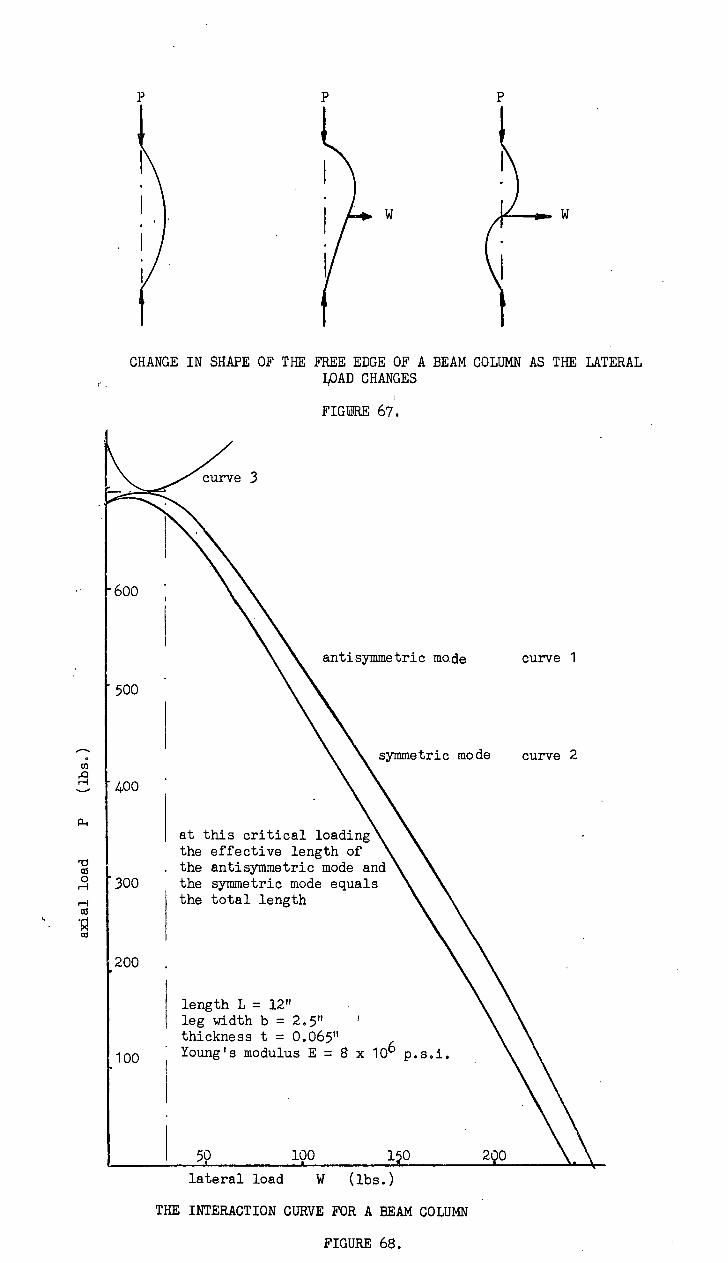
r-I
290
curve 3
600
antisymmetric mode curve 1
500
symmetric mode curve 2
at this critical loading the effective length of the antisymmetric mode and the symmetric mode equals the total length
axia
l lo
ad
200
length L = 12" leg width b = 2.5" thickness t = 0.065" Young's modulus E = 8 x 10⁶ p.s.i. 100
190
400
300
CHANGE IN SHAPE OF THE FREE EDGE OF A BEAM COLUMN AS THE LATERAL LOAD CHANGES
FIGURE 67.
lateral load W (lbs.)
THE INTERACTION CURVE FOR A BEAM COLUMN
FIGURE 68.
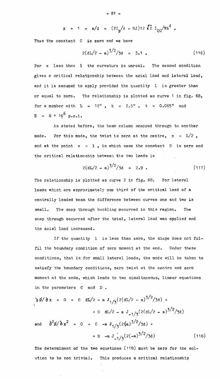
- 81 -
1. = a/d = (PI /A - GJ)12 17 IQQAb4 .
Thus the constant C is zero and we have
2(dL/2 - a) 3/2/3d = 3.1 • (116)
For x less than 1 the curvature is unreal. The second condition
gives a critical relationship between the axial load and lateral load,
and it is assumed to apply provided the quantity 1 is greater than
or equal to zero. The relationship is plotted as curve 1 in fig. 68,
for a member with L = 12" 9 b = 2.5" , t = 0.065" and
E = 8 x 10⁶
p.s.i.
As stated before, the beam column snapped through to another
mode. For this mode, the twist is zero at the centre, x = L/2
and at the point x = 1 , in which case the constant D is zero and
the critical relationship between the two loads is
2(dL/2 - a) 3/2/3d = 2.9 . (117)
The relationship is plotted as curve 2 in fig. 68. For lateral
loads which are approximately one third of the critical load of a
centrally loaded beam the difference between curves one and two is
small. The snap through buckling occurred in this region. The
snap through occurred after the total, lateral load was applied and
the axial load increased.
If the quantity 1 is less than zero, the shape does not ful-
fil the boundary condition of zero moment at the end. Under these
conditions, that is for small lateral loads, the mode will be taken to
satisfy the boundary conditions, zero twist at the centre and zero
moment at the ends, which leads to two simultaneous, linear equations
in the parameters C and D
= 0 = C dL/2 - a J113
(2(dL/2 a) 3/2/3d) +
+ D dL/2 - a J-1/3(2(dL/2 - 03/2/3d)
and 4 20/ x2 = C -a J
1/3(*) 3/2/3d) +
+ D -a J.0 /3 (2(-a) 3/2/3d) -
(118)
The determinant of the two equations (118) must be zero for the sol-
ution to be non trivial. This produces a critical relationship

axia
l lo
ad
.600 ,
leg width b = 2.5" length L = 24" thickness t = 0.065" Young's modulus E = 8 x 10⁶ p.s.i.
-4.00 Y experimental points
300
200
_ 100
20 40 60 80
lateral load W (lbs.)
APPROXIMATE INTERACTION CURVE FOR A BEAM COLUMN
FIGURE 69.
-500
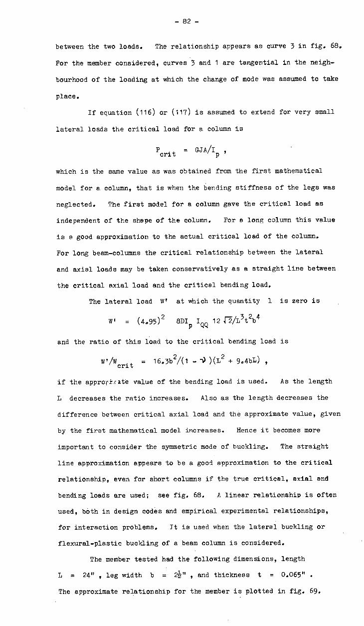
- 82 -
between the two loads. The relationship appears as curve 3 in fig. 68.
For the member considered, curves 3 and 1 are tangential in the neigh-
bourhood of the loading at which the change of mode was assumed to take
place.
If equation (116) or (117) is assumed to extend for very small
lateral loads the critical load for a column is
Pcrit
= GJA/Ip
which is the same value as was obtained from the first mathematical
model for a column, that is when the bending stiffness of the legs was
neglected. The first model for a column gave the critical load as
independent of the shape of the column. For a long column this value
is a good approximation to the actual critical load of the column.
For long beam-columns the critical relationship between the lateral
and axial loads may be taken conservatively as a straight line between
the critical axial load and the critical bending load.
The lateral load WI at which the quantity 1 is zero is
W I 1---/
= (4095) 2 8DIp
IW
12 42/1, 3 t 2 b4
and the ratio of this load to the critical bending load is
410/Wcrit
1603102)
( - 1) )(L2 + 9 0 410L) 9
if the appro(late value of the bending load is used. As the length
L decreases the ratio increases. Also as the length decreases the
difference between critical axial load and the approximate value, given
by the first mathematical model increases. Hence it becomes more
important to consider the symmetric mode of buckling. The straight
line approximation appears to be a good approximation to the critical
relationship, even for short columns if the true critical, axial and
bending loads are used; see fig. 68. A linear relationship is often
used, both in design codes and empirical experimental relationships,
for interaction problems. It is used when the lateral buckling or
flexural-plastic buckling of a beam column is considered.
The member tested had the following dimensions, length
L = 24" , leg width b = 2i" , and thickness t = 0.065" .
The approximate relationship for the member is plotted in fig. 69.

- 83 -
The member may be considered as a long member. The experimental
values are also plotted,and are less than the values given by the
mathematical model.
In the previous calculations, the central lateral load has been
applied so that the free edge of the leg is in compression. In the
case of a centrally loaded beam with the free edge in tension the beam
fails by plastic collapse. Thus the question arises, "What is the
behaviour of a beam column when a negative moment is applied so the
extreme fibre, is in tension?" This question will not be answered
here, although it is obvious that both the buckling mode and the
plastic failure due to bending will have to be considered. In con-
sidering the buckling properties, new modes will have to be invest-
igated. For the plastic analysis, an estimate of the moment must be
made. A suitable first approximation might be
/ wL/4 + PWL3 /48E10 - M
where PE is the flexural, Euler buckling load.
Returning to the general problem, we may note that the poss-
ibility of the beam-column failing by flexural or lateral-torsional
buckling or plastic failure should be considered. Taking the
problem one step further, the interaction between the modes could be
considered.
SUMMARY
A detailed mathematical model has been developed in this
thesis to describe the behaviour of a point loaded cantilever. The
estimated shapes and critical loads agree well with the measured
values. This model has been extended to cover a centrally loaded
simply supported beam and a laterally loaded column. However, the
beams and laterally loaded columns have the difficulty that more than
one mode exists. As already pointed out the two modes of the beam are
thought to depend upon the initial shape and the loading of the beam.
It is also probable that the mode depends upon the dimensions of the
beam, especially the leg width-length ratio.
The critical load of a beam is virtually independent of the
length of the beam for most practical members. It also appears that

- 84 -
the lower limit of the critical, maximum moment is independent of the
way in which the beam is loaded. The following conditions can be
used as conservative design criteria:
for a column the axial stress
dacrit
GJ/I
for a beam the maximum bending stress Cmcrit
= E(t/b)2/(1 +1) )
and for a laterally loaded column 6/6.a + 6m/6121i
. 1 . crit crt
The mathematical model for a laterally loaded column is very limited
in its application and the problem needs more consideration, but it
appears from the model developed that the linear relationship between
the axial and bending stresses is sufficiently accurate for design
purposes.
It should be emphasized that this chapter has introduced many
unsolved problems and the ideas presented are only a guide to the
fundamental understanding of the problem. Problems which arise from
the work done are the non-elastic buckling modes and loads, the inter-
action of the lateral and local buckling modes of beams, general load-
ing of beams, flexural-torsional buckling of laterally loaded columns,
and also the effect of opposing lateral and axial loads. The math-
ematical solutions of most of these problems will involve complex
mathematical models, which will be of little practical benefit, and
thus it appears that the expressions for the stresses in this summary
are good design criteria.

CONCLUSIONS
In this chapter four topics will be considered. The relation-
ships between the mathematical models developed in this thesis and
those developed previously will be discussed,and it will also be shown
how these mathematical models can be extended to apply to a general
cross-section. The design codes established as a guide in designing
members of the type will be studied and the unanswered questions
rising from the work carried out will be stated and possible lines of
attack will be suggested. Mention will also be made of plastic
buckling, although this topic has only been touched upon in the thesis.
Timoshenko1has considered the torsional buckling of short,
equal leg, angle-section members. He arrived at la simple mathematical
model, called the first mathematical model in this thesis. He also
derived a more complex model which included the plate stiffness of the
member. The angle-section member was considered as two flat rect-
angular plates buckling under a uniformly distributed compressive load.
The assumed boundary conditions were that the line of shear centres
remains straight and that this line acts as a pin-joint between both
legs, as the moment m round the corner is zero, The ends of the
member were assumed to be pin-jointed. The problem then reduced to
one of the buckling of a rectangular, flat plate with one free edge
and three pin-jointed edges, under uniform compression in the axial
direction x • In fact it was assumed that any change in the long-
itudinal stresses Nx
due to the deformations was negligible and the
stresses were taken as constant and equal to the ratio of the force P
to the cross-sectional area A .
The deflections w normal to the leg were taken to be of the
form
w = f(y) sin (Tlx/L) ;
where f(y) is a function of y only, and w satisfies the boundary
conditions at x = 0 L • If w satisfies the equilibrium
equation for a plate element,
b,4w/ x4 + 2 !• 41801 x2 y2 + 40s y4 = Nx/D 2vi/b x2
then w = A(cosh y + B sinh (Sy) sin7rx/L
!,.‘t Ref. 1 S. P. Timoshenko: "Elastic Instability".

-86-
for a unique load given by
P = 2mD/b
where D is Et 3/12(1 - -) 2) is the flexural rigidity, E is Young's
modulus, 7) is Poissons ratio, t is the leg thickness, and m is
a parameter which depends upon the ratio of the length of the member
L to the leg width b and the elastic properties of the material.
For a Poisson's ratio of 0.3 the constant m becomes
= 0.425 + b 2/L 2
Bleich has made a detailed survey of the local buckling of
columns of general cross-section. He treats each leg of the member
as a plate with either one or two elastic supports. The coefficient
of restraint of the support depends upon the neighbouring elements.
The analysis includes both an elastic and an inelastic treatment.
For an inelastic material the elastic modulus is replaced by the tan-
gent mo.-.1u=4. It was also assumed that the ratio of the tangent and
elastic moduli is the same for both shear and normal deformations
at any given axial loading. Bleich treats equal-leg angle-section
members as a special case. The average critical stress is
= prr 2E ff. ( fib ) 2 ( ss: (b/1) 2 + 0 0 425)/12(1 -1) 2 )
(119)
for -1) = 0.3 .
Bulson also gives a detailed analytic treatment for local
buckling of thin, open section members. He gives the experimental
results he obtained and compares them with the analytic results. For
a member which buckles inelastically, he suggests an average modulus
El (where Et
is the tangent modulus and Esec
is the secant modulus)
given by
E' - i - 4Et+E sec
The expression for the critical load of a member buckling
torsionally, derived in this thesis is
= E(t/b ) 2 ((b/1) 2 + 6(1 )/Te2)/12(1 - -) 2 ) . (120)
When a Poisson's ratio of 0.3 is considered the expression is
identical to the one obtained by Timoshenko and Bleich l (equation

— 87 —
119). However, it •has the advantage that it is simply derived and
the value of the constant m can be readily evaluated for various
Poisson's ratio values.
Bleich also discussed the thickness of plates required so
that a column fails by flexural buckling before local buckling
occurs. The inequality expressing this condition is
( 1171) 2Eb3t/12 = 1r 2E/(1/p) 2 4: Tr 2E/12(1 .4 2 )(t/b)((b/1 2
-I- 0.425)
"= k(t/b) 2IY2E/12(1 - -V 2 )
Or t/b 45. C 1-7C 9 (121)
where C is a function of the slenderness ratio Vivo Bleich also
extends the inequality for inelastic buckling, by assuming a linear
relationship between C and the square root of the slenderness ratio°
For equal leg, angle section members Bleich gives
b/t !I 0.6520 o
The Column Research Council Guide to Design Criteria for
Metal Compression Members states that the American Institution of
Steel Construction bases its code for local buckling on any supported
edge being simply supported and that a local buckling must not form
before the material yields, which gives the yield stress
igY= (t/b) 2 2E/12(1 - -02 )((0/1) 2 0.425)
for an outstanding leg. For a steel with a yield stress of 36kpsi the
2 allowable leg width—thickness ratio is 17.6. A.I.S.C. practice gives
the limits:
for an outstanding leg: b/t .1= 3000/1Z
and for an element supported along each edge:
b/t 8000/1-47
The German code DIN 4114 follows the same attitude as was used
by Bleich, and designs the column so that local buckling does not occur
Ref. 1: F. Bleich "Buckling Strength of Metal Structures" Ref. 2: American . Institute of Steel Construction, "Manual of Steel
Construction".

- 88 -
before overall buckling. The code states, for the outstanding leg;
if the slenderness ratio 1/p.> 75 then b/t = 0.2 i/p else
b/t = 15 .
For a member supported along each edge, a table is provided, in
which a formula for the permissible ratio is quoted. The ratio
depends upon the shape and dimensions of the overall cross-section.
The code also allows for the stiffness of the joints between two
con tituent plates.
The British Code BS449 1959 gives a formula for the following
ratio for the three steels mentioned. The ratios are based upon the
yield criteria. For steel BS15 the allowable leg width thickness
ratio is sixteen, for BS548 and 968 the ratio is fourteen. The draft
(1966) for the Australian Code SAA Inst. 351 uses the AISC formulae
for the detailed design of compression members.
The American Society of Civil Engineers1suggested specifications
for different aluminium alloys. In determining the allowable dim-
ension of members governed by local buckling of the constituent
elements it is assumed that all supported edges are simply supported.
This is conservative.
Few codes consider the local buckling of a leg with non uni-
form stress. However the ASCE committee has included the cases when
a member is bending about the minor or major axis. Timoshenko has
solved the problem of the buckling of a plate with linearly distrib-
uted longitudinal stresses using an energy approach. The mathematic-
al model developed in this thesis gives the maximum allowable bending
stress in a cantilever or centrally loaded simply supported beam as
6 . Mb/2 0 1QQ = WcritL/8 IQQ
E(0) 2(1 + 9 0 4b/L)/(1 +1))
For large L a conservative allowable stress is
E(t/b) 2/(1 +70) or 1r 2E(b/t) 2/(305) 2 (122)
which is the value quoted by the ASCE committee. This value is also
a conservative estimate for a beam bending under a uniform bending
Ref. 1 Proc. Am. Soc. of Civ.. Eng. Journal of Structural Div.AVo1..88 Dec. 62, "Suggested.Specifications for Aluminium Alloy'.

- 89 -
moment as for that loading
(E(t/b) 2/(1 +1)))(1 +11#2 (b/L) 2/6(1 -1))) .
In fact equation (122) is conservative estimate of the stress for all
beams.
When an angle section member is loaded about the major axis a
conservative assumption would be to assume each leg was simply support-
ed and the stress varied linearly from zero to a maximum, which gives
an allowable stress of
di= 1eE(t/0 2/(4.4) 2 (123)
for long members.
In the work presented previously it be assumed that the root
of the angle-section member is weak and the included angle changes
when a moment is applied about the major axis. Most extruded or
rolled sections have a fillet, which strengthens the root of the angle.
Consequently the tendency will be for the included angle to be main-
tained and for the legs of the cross-section to deform. It is poss-
ible to analyse this functional form by considering each plate sep-
arately and applying compatibility of statics and geometry at the root.
When the functional form is taken to be rotation of the cross-section
in an undeformed state, bending about the major axiL does not cause
torsional instability. The experimental analysis of beams has been
limited to bending about the minor axis. Bending about the major
axis can be considered by either of the methods described above,
although it is reasonable to assume that the true functional form is a
combination of the two forms.
All the design codes quoted are based on a conservative
estimate of the load capacity of a member. The mathematical models
developed by the author allow for a less conservative design of both
beams and columns, with very little extra computation. However in the
case of a general bbam, it is unlikely that the differential equations
which are derived from the mathematical model will prove se.vable.
Flexural-torsional buckling of thin-open section members in
compression has been studied in some detail by Timoshenko, Weber,
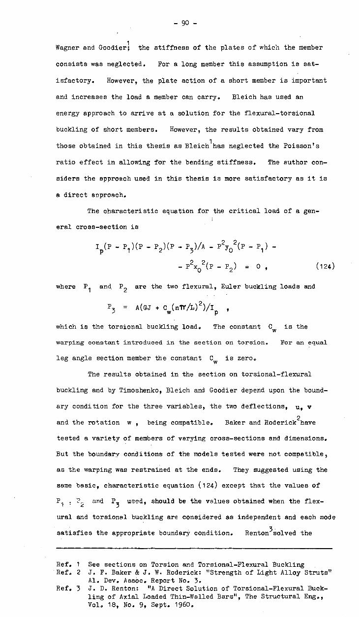
- 90 -
1 Wagner and Goodier; the stiffness of the plates of which the member
consists was neglected. For a long member this assumption is sat-
isfactory. However, the plate action of a short member is important
and increases the load a member can carry. Bleich has used an
energy approach to arrive at a solution for the flexural-torsional
buckling of short members. However, the results obtained vary from
those obtained in this thesis as Bleich1has neglected the Poisson's
ratio effect in allowing for the bending stiffness. The author con-
siders the approach used in this thesis is more satisfactory as it is
a direct approach.
The characteristic equation for the critical load of a gen-
eral cross-section is
I (P - P1 YO - )(P - P 2 )(P - P 3)/A - P2 2(P P ) -
P 1
- P2x02 (P - P2 ) = 0
(124)
where P 1 and P 2 are the two flexural, Euler buckling loads and
/ \\ / P3 = A(GJ + Cw(n1r/L)
2)/I
which is the torsional buckling load. The constant Cw is the
warping constant introduced in the section on torsion. For an equal
leg angle section member the constant C w is zero.
The results obtained in the section on torsional-flexural
buckling and by Timoshenko, Bleich and Goodier depend upon the bound-
ary condition for the three variables, the two deflections, u, v
and the rotation w , being compatible. Baker and Roderick2have
tested a variety of members of varying cross-sections and dimensions.
But the boundary conditions of the models tested were not compatible,
as the warping was restrained at the ends. They suggested using the
same basic, characteristic equation (124) except that the values of
P ? and P3
ued, should be the values obtained when the flex- '. - 2
ural and torsional buckling are considered as independent and each mode
- satisfies the appropriate boundary condition. Renton 3 solved the
Ref. 1 See sections on Torsion and Torsional-Flexural Buckling Ref. 2 J. F. Baker & J. W. Roderick: "Strength of Light Alloy Struts"
Al. Dev. Assoc. Report No. 3. Ref. 3 J. D. Renton: "A Direct Solution of Torsional-Flexural Buck-
ling of Axial Loaded Thin-Walled Bars", The Structural Eng., Vol. 18 1 No. 9, Sept. 1960.

- 91 -
problem for any set of end conditions, both statical and geometric.
He compared his analytic results with Baker and Roderick's results.
The difference between Renton's mathematical model and the approximate
mathematical model is very small. The difference is most noticeable
for a T-section and angle section members.
Bleich gives some diagrams which show the susceptibility to
flexural and torsional-buckling of members having cross-sections of
various shapes. Only tee-members and the angle section members are
1 prone to torsional buckling. Bijlaard and Fischer, in discussing the
interaction between local and overall buckling, state: "The inter-
action effect is negligible for box sections as indicated by both
theory and experiment...; the same conclusions apply to common size
of H and channel sections, but not to sections for which torsional
instability is an important factor, such as the tee and angle sections".
One of the conditions for calculating the critical loads for
the various types of buckling was that the mode being investigated
predominated. In the case of local buckling it WPS assumed the line
of shear centres remained straight. In the case of torsional-flexural
buckling it was assumed the cross-section did not distort.
A. Chajes and G. Winter2have arranged the torsional-flexural
model into a form suitable for a design office tool. The critical
load P for a cross-section with one axis of symmetry can be expressed
as
P/P1 + P/P
3 - KP2/P1
P3
. 1
( 1 2 5)
where P1 and P3
are the flexural and torsional critical loads and
K is a factor which depends only upon the geometry of the cross-
section. He also gives the values of the torsional load P 3 .the
constant K, and the type of failure as graphs plotted against a non-
dimensional parameter of the cross-section.
Most codes mention that a column should be checked for torsion-
al instability. However, only Addendum No. 1 (1961) to the British
Ref. 1 Column Research Councils Guide to Design Criteria for Metal Compression Members.
Ref. 2 A. Chajes and G. Winter, Proc. A.S.C.E. Struct. Vol. 9 1 , Aug. 1965.

- 92 -
Code BS499 tackles the problem numerically. A table of equivalent
slenderness ratios 1/p are quoted for various cross-sections. Also
the Joint Committee of the British Instruction of Structural Engineers
and the Institute of Welding mention torsional buckling in their report
on "Fully rigid multi-storey steel frames". They set limits on the
distribution factor at a joint so that sufficient restraint is
provided to overcome torsional instability.
When a column is loaded laterally a straight line interaction
curve is usually considered sufficient,
p/pult
+ M/Mult
1
(126)
where Pult and Mult are the load capacity of the member under an
axial load P and as moment M respectively. This is the case for
the local buckling of the member. However, in general the ultimate
moment can either be the lateral buckling load, plastic moment or the
moment to cause local buckling. Curves of the form
P/Pult + M/(K Mult
(1 - P/Pult
)) 1
or P/Pult
+ (M/Mu1t
) 2/K
(127)
have also been considered. The first alternative is quoted in some
codes, for example the AISC Manual of Steel Construction. The second
alternative is used in connection with lateral buckling,and also as an
upper bound on the true load capacity. The work in this thesis
indicates that the linear relationship is a good approximation for local
buckling.
The large deflection, elastic model for the torsional instabil-
ity of a column indicates that an elastic member is able to carry a
load greater than the critical load, if the deformations are not
important. However, the increased load capacity of the member
decreases as the leg width-thickness ratio decreases. If we consider
an initially straight member end denote the increase in load above the
critical load at which a unit twists is achieved by P, then the
ratio of the increase to the critical load P is crit
P i/P rit
(1 -1))b2(b/t)/40((b/1) 2 2 + 6(1 -1)))
If the thickness is increased or the leg width decreased the ratio

— 93 —
decreases.
This thesis has not considered the behaviour of a member once
the material becomes plastic. Most design codes are based upon the
Bleich approach of replacing the modulus of elasticity by a "modulus
of plasticity". The codes also include an empirical expression for
the ratio of the two moduli r . One of the most interesting facts
observed is that all members tested, whether as beams or columns,
failed in the same plastic "triangular" mode (figs. (61), (51) and
(38). However as pointed out, this functional form cannot be used to
obtain an upper bound on the load capacity, as it appears that the
member has partially unloaded before the true "triangular" mode is
formed.
Codes also take into account the load capacity of a member in
which a local buckle has occurred. But the suggested specifications
of the ASCE specifically state that single angle, double angle,
crucifix and tee members should not be included, their reason being
that the interaction between local buckling and overall buckling is
important for these sections. The effective leg width for other
sections is taken as a fraction of the leg width which depends upon
the load being carried and the critical load to cause local buckling.
The effective leg width is used in calculating the load capacity of the
member.
In all the mathematical models developed in this thesis, the
change of loading as the deformations increase has been neglected. In
the case of both the cantilevers and the beams tested the direction of
the load was independent of the deformations. The beams were loaded
through the shear centre and although the mathematical models
describing the local buckling is not effected by the way the model is
loaded, when the lateral buckling of the beam is considered this is
important.. For large deflections of an eccentrically loaded column,
it is thought that the bearing stresses on the base redistribute in
such a manner as to increase the eccentricity and consequently stiffen
the model. The discrepancy between the measured and the estimated
graph in Fig. 33 could be explained by this fact.

— 94 —
All the members investigated have been tested as single members,
and have not been integrated into a truss. Thus the problem rises as
to how a member acts in a. truss. The primary problem is the boundary
conditions. Both the beams and the columns have been considered as
pin-ended. While it would appear reasonably simple to consider a
column with any boundary conditions, the boundary conditions of a
laterally loaded beam would be more difficult to apply, especially as
the mode is complex and it is possible to obtain two modes. Already
the possibility of including the variation of the torsional strength of
a member with the axial load and end moment to the overall buckling of
a frame has been mentioned. However, the problem is not as serious
as it first appears as the critical load, both for long columns and
long beams, is independent of the length.
Other applications of angle section members must be considered.
Often two angles are bolted together to act as a strut. The local
buckling of the individual angle members can be considered by using
the mathematical models developed. However, in considering the
overall torsional and flexural buckling of the member, the member must
be considered as a tee-member. The problem of double bulb angle
struts is considered by Cullimore.
The torsional buckling of a member about a fiyed axis of
1 rotation is considered by Bleich. Maurice Sharp
2investigates the use
of longitudinal stiffeners on flat angle, one application of angle-
section member. If a lip is added to the free edge of the leg of the
angle member the load capacity of the member is increased. Bulson3
discusses analytically the effect of lips on cross-section. Sharp
also includes the action of a lip in his paper.
The last section of this chapter has been devoted to common
applications of angle-section members. All the references quoted have
treated the problem using the classical approach. It is quite poss-
Ref. 1 F. Bleich "Buckling Strength of Metal Structures" Ref. 2 M. L. Sharp "Longitudinal Stiffness for Compression Members"
Proc. Am. Soc. of Civ. Eng., Struct. Div., October 1966. Ref. 3 P. S. Bulson "Local Instability Problems of Light Alloy
Struts". Al. Dev. Assoc. Report No. 29.

— 95 —
ible to attack these problems in the same manner as used in this
thesis, and the author feels that, as a result, a more simplified
mathematical model can be obtained, based upon a clear understanding
of the problem.
While the mathematical models developed by the author have in
general not broken new ground, the approach used has enabled an
examination to be made of the local buckling of all structura:members
using basically the same functional form for the geometry, the same
underlying ideas, and similar mathematical models. The author feels
that this approach is of benefit, as the review of existing literature
on this topic has shown that many different approaches are required to
cover the topics considered, ane; roost of these approaches involve
complicated and somewhat abstract mathematics. The geometric
approach will be of particular importance when more complex problems
are considered. For these problems an advanced numerical or
algebraic analysis of each member will most likely have to be used,
The geometric functional form approach can be simply and logically
applied to these problems.

APPENDIX A
ELASTIC BENDING OF THIN PLATES
In the following section of the thesis, the mathematical model
of bending of thin plates is developed. The results obtained have
been applied repeatedly throughout the thesis. The analysis closely
follows the lines followed by Timoshenko1except that some of the
symbols have been defined differently. The model is based upon the
fact that all the strains vary linearly across the section, that is,
throughout the thickness. The model includes the case when the
centre plate deforms.
The coordinate system with which the model will be developed
will be x, y axes in the plane of the unloaded plate and the z
direction normal to the x-y plane. The deflections in the z
direction will be denoted by w . (see fig. 29) The element to be
considered is of thickness, t and defined by the planes x, x+ax, y
and yvly . The following notation will be used
N N longitudinal stresses on the central plane x y
shear stresses on the central plane xy
normal shear stresses Qx Qy
m bending moments about x and y axis x y
and m twisting moments xy
All symbols are quantities per unit length.
thickness
flexural rigidity, D Et 3/12(1 -7) 2 )
and KK curvatures x y
The symbols are defined graphically in fig. 29.
In general the shape of the plate is known, so that the aim
will be to develop expressions for the internal actions of the plate
in terms of known geometry using the load deformation relationship.
In the case of small deflections the change in the curvatures is
Kx 2w/x2
and K ?3 2wA y2
Ref. 1 S. P. Timoshenko "Plates and Shells", McGraw-Hill Book Co., Inc.

Nxi4NWey dy /e) dy •
Y Y Y
thxy+ /e5r-
Nxv+bN dY Q-.
dy
Nx + )3N3dx dx
All cuts are parallel to the x, y, z axes.
All forces are parallel to the x,y and z axes.
Thickness of element t
Qx) Qy shear forces
Nx) longitudinal forces m 0 m,m moments.
x y xy
All forces are forces per unit lengths
FORCES ON AN ELEMENT dx dx t
FIGURE 29

- 97 -
and the change in twist is
K = 2w/x xy
If the problem is further restricted and only linear load deformation
relationships are considered, that is the materials are elastic, the
moments per unit length required to maintain the deformations are
D( 2vv/ x2 .142w/e,y2) mx - D(K +1)K ) x y
- D(K +1)K ) D( 12w/ y2 VwRi x2 )
y x
and m D(1 -1)) )2u0 y 6x = K D(1 - 1) ) . xy xy
The internal shearing stresses can be obtained by considering
the equilibrium of an element of the plate. The equations of
equilibrium are
force equilibrium in the z direction
1 Qx/ y + Qy/ x = o
force equilibrium in the x direction
?$Nxy/6 y + )sNd x = 0 ,
force equilibrium in the y direction
+ 6N3 /6 y = 0 9
moment equilibrium in the zx plane
Qx = m3di x - ?)mxy/ è y — Nx w/ 6 x - N y
moment equilibrium in the zy plane
Q = m y — 6m /6x - N w/ y - N 6 w/ 6 x .
xy xy
The equilibrium equations in conjunction with the load deformation
relationships give an expression for the shearing forces for unit
length in terms of the geometry,
Q = - D( ?3:5',16 x3 + •310 )c) y2 ) - (1 -1) )D . 30o y2 ie3 x - x
- N x — N w/6 y xy
and
= - ]D( 30 Y3 x2)3 Y) - - 1) )1) e3viii 3,2 - Y
_ N y - N xy

— 98 —
It should be noted that although the final expressions depends upon
having small deflections and a linear mode deformation relationship,
the equations of equilibrium are independent of both these
restrictions.

APPENDIX B
Solution of the differential equation, third model for a
column loaded through a base plate
20/63c2 +.0.20 — t‘ p = u •
Multiply by 2 00) x ;
2 x V0/ x 2 + 21'00 2:4 x - 2 p 95/?) x = 0
After integrating with respect to x the equation becomes
( 0/ 6 )02 4. ..0.202 2/3 (504 c
Or PS/)37C = (C 02 (11-2 — 2/302 ))4 .
Properties of the elliptic functions
f • 2 \ cnz = k1 - Sn zr 9
22 1
dnz = (1 - k sn z) 2
dsnz/dz = cnz dnz
denz/dz = - snz dnz
d dnz/dz = - k 2 snz dnz
and d 2 snz/dz2 k2 sn3z - k
2 snz - snz + k2
sn3 z
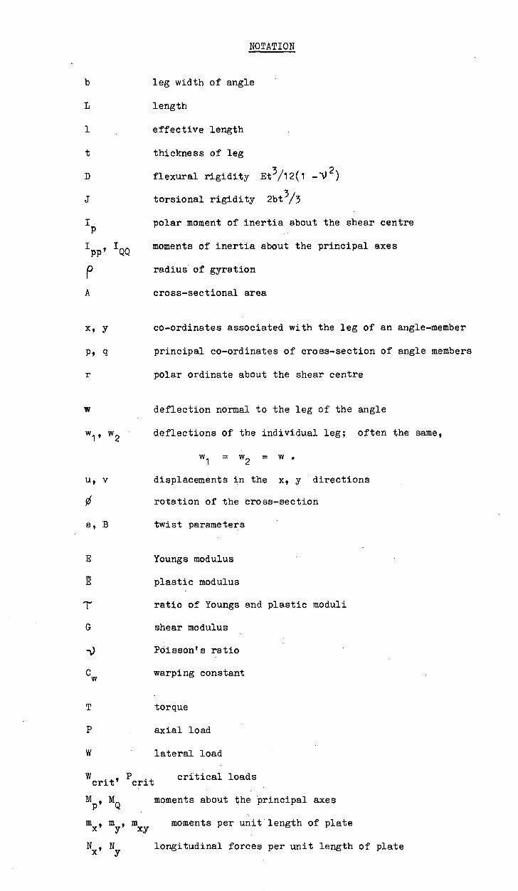
NOTATION
leg width of angle
length
1 effective length
thickness of leg
flexural rigidity Et 3/12(1 - 10 2 )
torsional rigidity 2bt 3/3
polar moment of inertia about the shear centre
IPP,
IW
moments of inertia about the principal axes
radius of gyration
A cross-sectional area
X9 y co-ordinates associated with the leg of an angle-member
Pt q principal co-ordinates of cross-section of angle members
polar ordinate about the shear centre
deflection normal to the leg of the angle
W.1 w2 deflections of the individual leg; often the same,
w 1 = w2 = w
U 9 V
displacements in the x, y directions
rotation of the cross-section
a, B
twist parameters
Youngs modulus
plastic modulus
1- ratio of Youngs and plastic moduli
shear modulus
1) Poisson's ratio
Cw warping constant
torque
axial load
lateral load
critical loads Wcrit' crit
M MQ
moments about the principal axes P 9
m 9 m, m moments per unit length of plate x y xy
N N longitudinal forces per unit length of plate x y

-
N shear force per unit length of plate xy
Q , Q shear forces per unit length plate acting a cross the x y
thickness of the plate
K 9 K curvatures in x and y directions x y
twist xy
strain
cr stress
eccentricity
X eigen value
potential energy