stability of collaborative filtering recommendation

Stability of Collaborative Filtering Recommendation Algorithms1 GEDIMINAS ADOMAVICIUS, University of Minnesota

JINGJING ZHANG, University of Minnesota The paper explores stability as a new measure of recommender systems performance. Stability is defined to measure the extent to which a recommendation algorithm provides predictions that are consistent with each other. Specifically, for a stable algorithm, adding some of the algorithm’s own predictions to the algorithm’s training data (for example, if these predictions were confirmed as accurate by users) would not invalidate or change the other predictions. While stability is an interesting theoretical property that can provide additional understanding about recommendation algorithms, we believe stability to be a desired practical property for recommender systems designers as well, because unstable recommendations can potentially decrease users’ trust in recommender systems and, as a result, reduce users’ acceptance of recommendations. In this paper, we also provide an extensive empirical evaluation of stability for six popular recommendation algorithms on four real-world datasets. Our results suggest that stability performance of individual recommendation algorithms is consistent across a variety of datasets and settings. In particular, we find that model-based recommendation algorithms consistently demonstrate higher stability than neighborhood-based collaborative filtering techniques. In addition, we perform a comprehensive empirical analysis of many important factors (e.g., the sparsity of original rating data, normalization of input data, the number of new incoming ratings, the distribution of incoming ratings, the distribution of evaluation data, etc.) and report the impact they have on recommendation stability.

Categories and Subject Descriptors: H.3.3 [Information Search and Retrieval]: Information Filtering, H.2.8.d [Information Technology and Systems]: Database Applications – Data Mining, I.2.6 [Artificial Intelligence]: Learning.

General Terms: Algorithms, Measurement, Performance, Reliability.

Additional Key Words and Phrases: Evaluation of recommender systems, stability of recommendation algorithms, performance measures, collaborative filtering.

1. INTRODUCTION AND MOTIVATION Recommender systems analyze patterns of user interest in order to recommend items that best fit users’ personal preferences. In one of the more commonly used formulations of the recommendation problem, recommendation techniques aim to estimate users’ ratings for items that have not yet been consumed by users, based on the known ratings users provided for consumed items in the past. Recommender systems then recommend to users the items with highly predicted ratings. Recommender systems can add value to both users and companies [Dias et al. 2008; Garfinkel et al. 2006; Legwinski 2010; Rigby 2011] and are becoming an increasingly important decision aid in many information-rich settings, including a number of e-commerce websites (e.g., Amazon and Netflix).

Much of the research in recommender systems literature has focused on enhancing the predictive accuracy of recommendation algorithms, although in the last several years researchers started to explore several alternative measures to evaluate the performance of recommender systems. Such metrics include coverage, diversity, novelty, serendipity, and several others, and comprehensive overviews of different metrics and key decisions in evaluating recommender systems can be found in [Herlocker et al. 2004; Shani and Gunawardana 2011]. Our work follows this general stream of research in that we believe that there are other important aspects of recommender systems performance (i.e., aside from accuracy) that have been largely overlooked in research literature. In particular, in this paper we introduce and explore the notion of stability of recommendation algorithms, which we first illustrate and motivate with the following simple example (also depicted in Figure 1).

Suppose we have a movie recommender system, where user Alice has entered the ratings 4, 2, 1 (on the scale from 1 to 5) into a recommender system for the three

1 This paper substantially augments and improves its preliminary version which appeared in ACM RecSys 2010 [Adomavicius and Zhang 2010].

movies that she saw recently and, in return, the system provided for her the following rating predictions for four other movies: 4, 4, 5, and 1. Following the recommendations, Alice went to see the first three of the movies (because they were highly predicted by the system), but avoided the fourth one (because it was predicted only as 1 out of 5). It turns out that, in Alice’s case, the system was extremely accurate for the three movies that were predicted highly, and Alice indeed liked them as 4, 4, and 5, respectively. Imagine Alice’s surprise when, after submitting these latest ratings (which were exactly the same as the system’s own predictions), she saw that the recommender system is now predicting the final movie for her (which earlier was 1 out of 5) as 5 out of 5.

Figure 1. Example scenario of unstable recommendations.

A regular user like Alice, who ended up providing ratings for the three movies

exactly as predicted by the system, therefore, may initially be quite impressed by how well the system was able to understand and predict her preferences for these movies. However, the subsequently observed instability in rating predictions (i.e., internal inconsistency of the recommendation algorithm) may seem especially odd and confusing. Providing consistent predictions has important implications on users’ trust and acceptance of recommendations. For example, it has been shown in the consumer psychology literature that online advice-giving agents with greater fluctuations in past opinions are considered less informative than those with a more uniform pattern of opinions [Gershoff et al. 2003]. Also advice that is inconsistent with past recommendations is considered less helpful than consistent advice [d’Astous and Touil 1999; Van Swol and Sniezek 2005]. Inconsistent recommendations provided by recommender systems may be discredited by users and, as a result, the downgrade in users’ confidence can directly reduce users’ perception of system’s personalization competence. For example, previous studies found that user’s trust and perception of personalization competence are the keys that lead to user’s acceptance of recommendations [Komiak and Benbasat 2006; O’Donovan and Smyth 2006; O’Donovan and Smyth 2005; Wang and Benbasat 2005]. Hence the instability of a recommender system is likely to have potential negative impact on users’ acceptance and, therefore, harm the success of the system.

We would like to note that the recommendation example described in Figure 1 is not a purely hypothetical scenario – this can happen to some of the popular and commonly used recommendation algorithms, as will be discussed later in the paper. To define the notion of stability more precisely, we formalize the procedure used in the above example. Specifically, we measure the stability of a recommender system as the degree to which the system’s predictions for the same items stay the same (i.e.,

stay stable) over time, when any and all new incoming ratings submitted to the recommender system are in complete agreement with system’s prior predictions. Intuitively, (in)stability of a recommendation algorithm represents the degree of (in)consistency between the different predictions made by the algorithm. In other words, two predictions of the same recommender system can be viewed as “inconsistent” with each other, if accepting one of them as the truth (i.e., if the system happens to be perfectly accurate in its prediction) and adding it to the training data for the system changes (invalidates) the other prediction. By our definition, stable systems provide “consistent” predictions and vice versa.

Figure 2 provides a very simple illustration of stable vs. unstable recommendation techniques, T1 and T2. Suppose, for a given user, the two techniques start with the same exact predictions for unknown items, but adding new ratings that are identical to system’s prior estimations leads to different predictions on remaining unknown item set. For a stable technique T1, adding new ratings does not change the estimations on other unknown items. However, for an unstable technique T2, the addition of new incoming ratings can lead to a dramatic change in estimations for remaining unknown ratings. The extent of this change provides an opportunity to measure the degree of instability (and not just to determine if the technique is stable or not), and the formal definition of this measure is provided in the next section.

Figure 2. Illustration of stable and unstable recommendation techniques.

Understanding stability is important both from theoretical and practical

perspectives. The level of instability is an inherent property of recommendation algorithms because the measured changes in predictions are due to the addition of new incoming ratings which are identical to system’s previous estimations. As will be shown in the paper, different recommendation algorithms can exhibit different levels of instability, even though they may have comparable prediction accuracy. Therefore, it is important to understand inherent behavior of computational techniques that are used for predictive purposes in real-world settings. Also, it should be of value for recommender system designers to be aware how (un)stable various recommendation techniques are, especially since the stability may potentially have implications with respect to users’ trust and confidence in recommender systems, as discussed earlier. Therefore, we believe that stability constitutes an important complementary measure of recommendation systems performance.

The remainder of the paper is organized as follows. Section 2 formally defines the notion of stability and describes the framework for measuring stability of recommendation algorithms. Section 3 describes the experimental setup (datasets, recommendation techniques, etc.) used to obtain empirical results. Section 4 reports

and discusses the results of our comprehensive empirical stability-related investigations; in particular, we investigate the stability properties of several families of popular collaborative filtering recommendation algorithms and explore a number of data-related factors and their impact on stability. Section 5 discusses some related work, and the conclusions of the study are presented in Section 6.

2. DEFINITION OF STABILITY Before discussing the notion of stability, we briefly introduce some of the notation used in the paper.

Let Users be the set of all users in a recommender system and Items be the set of all items that can be recommended. Thus, we define a recommendation space S = Users × Items. The usefulness or utility of any item i to any user u can be denoted as rui, which usually is represented by a rating (on a numeric, ordinal, or binary scale) that indicates how much a particular user likes a particular item. Thus, the job of a recommender system typically is to use the available information (such as known ratings of items already consumed by users, content attributes of items, demographic attributes of users) to predict or estimate ratings for items that the users have not yet consumed. In other words, the goal is to construct a predictive model f: S → Rating, where Rating is a totally ordered set representing the rating scale, in order to predict the unknown ratings, i.e., ratings for items yet to be consumed by the users.

Let D be some rating dataset, i.e., dataset representing the ratings that have been submitted by users to a recommender system. For notational simplicity, let SD (SD ⊆ S) represent the portion of recommendation space S that is covered by D. In other words, D = {(u,i,rui)|(u,i)∈SD, rui∈Rating}. The predictive model is then constructed by the recommender system using some estimation technique T (e.g., neighborhood-based collaborative filtering [Herlocker et al. 1999; Sarwar et al. 2001] or matrix factorization [Koren 2010] to make best predictions on unknown ratings based on the input data D. We will denote such predictive model as fT,D. For clarity, we will use rui to denote the actual rating that user u gave to item i, and for the system-predicted rating for item i that user u has not rated before, i.e., , , .

To measure the performance of recommender systems, much of the research has primarily focused on predictive accuracy of recommendations. Predictive accuracy metrics compare the estimated ratings against actual ratings and represent the closeness of recommender system’s predictions to user’s true ratings. A number of accuracy metrics have been proposed in recommender systems literature, with Mean Absolute Error (MAE) and Root Mean Squared Error (RMSE) being among the most popular and widely used. MAE measures the mean absolute deviation of the predicted ratings from actual ratings. RMSE measures the root value of mean squared error (MSE) of predicted ratings which is the amount by which predicted rating differs from user’s actual rating. Mathematically the two accuracy metrics are computed as below:

∑ | |,

| | , ∑ ,

| |

Here S* represents a subset of SD specifically reserved for evaluation purposes (i.e., test dataset, not used during the model building process). We use these measures to

report the accuracy performance of the investigated recommendation algorithms. As discussed earlier, we define the predictive model to be stable if its predictions

are consistent with each other or, in other words, if its predictions for the same items are consistent over a period of time, assuming that any new ratings that have been submitted to the recommender system over that period are in complete agreement with system’s prior predictions. Thus, stability is an inherent property of a recommendation algorithm and can be quantified by the degree of change in

predicted ratings when rating data is extended with new incoming ratings. Formally, this extension is defined as follows:

Definition 1 [fT,D−extension]. Given recommendation algorithm T, set of known ratings D, and the resulting predictive model fT,D, dataset D' is an fT,D−extension of D, if it satisfies the following two conditions:

(1) D' ⊇ D; (2) For any (u,i,r)∈D'\D, we have fT,D(u,i) = r.

In other words, D' is an extension of dataset D (i.e., D' has all the same known ratings as D) with additional incoming ratings submitted to the system that are identical to estimations made by predictive model fT,D. Different predictive techniques can have different levels of instability, and thus allows quantifying the level of instability.

Definition 2 [general (in)stability measure2]. Level of instability of predictive technique T on dataset D and its fT,D−extension D' is defined as:

,, ,

where U is the set of unknown ratings need to be estimated.

In other words, , , measures the aggregate difference in predictions made by recommendation algorithm T on the original data D and predictions made by the same algorithm T on the extended dataset D' (D' ⊇ D). Again, the only change from D to D' is that D' has some additional ratings that were perfectly accurately predicted by T. To obtain the comprehensive view of the stability, this aggregate difference in predictions is calculated across the predictions for the entire unknown portion of the rating space U = S\SD'.

According to the definition, the level of instability may depend on several factors, including the type of predictive technique T, characteristics of initial rating dataset D, characteristics of the extension dataset D' (i.e., a given dataset can have a huge number of possible extension datasets), and the characteristics of the evaluation dataset U. Later in the paper we provide a comprehensive empirical examination of a number of important factors and their impact on recommendation stability.

Measuring stability of a recommendation algorithm involves comparing predictions made at several points in time. Following our definition, we adopt a two-phase approach to compute the stability of a recommender algorithm, which is illustrated in Figure 3.

In Phase 1, given a set of known ratings D, a predictive model fT,D is built, and predictions for all unknown ratings are made and denoted as P1, where P1(u,i) represents a system-predicted rating for user u and item i. In other words, P1(u,i) = fT,D(u,i) for all (u,i)∈S\SD.

Then, a set of hypothetical (simulated) incoming ratings is added to the original set of known ratings D by assuming that the recommendation system predictions P1 were identical to users’ true preferences for unknown rating set S\SD. Therefore, in Phase 2, some subset P of predictions P1 is added as the newly incoming known ratings, and the set of known ratings becomes D' = D ∪ P. In other words, D' is constructed as an fT,D−extension of dataset D. Based on D', a second predictive model fT,D’ is built using the same recommendation technique T, and predictions on remaining unknown ratings (i.e., for S\SD') are made and denoted as P2. In other words, P2(u,i) = fT,D'(u,i) for all (u,i)∈S\SD'. 2 In this paper, stability is measured on a non-negative continuous scale, smaller values indicating more stable recommendation algorithms, larger values less stable recommendation algorithms. Therefore, for convenience, we also sometimes refer to this measure as instability (i.e., larger values – larger instability, smaller values – smaller instability).

Stability is then measured by comparing the two predictions, i.e., P1 and P2, to compute their mean absolute difference or root mean squared difference, which we call mean absolute shift (MAS) or root mean squared shift (RMSS), respectively. More formally, for each user-item pair (u,i) in the prediction list, the prediction difference is denoted by:

1 2( , ) ( , )ui P u i P u iΔ = − . Then the above mentioned stability measures are computed as:

MAS = ( )2

2( , )

1 uiu i P

P∈

Δ∑ , RMSS= ( )2

2

2

( , )

1 uiu i P

P∈

Δ∑

Figure 3. Two-phase approach for stability computation.

To illustrate the intuition behind the stability computation, consider an example

data set containing 10 2-dimensional data points as shown in Figure 4. In this example, given these 10 data points (xi,yi) ∈ R2 , we are trying to build predictive models to predict y = f(x) for the entire space, i.e., for any x ∈ R. Lines in Figures 4a, 4b, and 4c depict model-based techniques (represented by 0-, 1-, and 2-degree polynomials, respectively) that fine tune their parameters (i.e., the coefficients of polynomials) using global optimization to fit the data in a way that minimizes sum of squared errors. For example, Figure 4a represents the best model of the form f(x) = b0, where b0 is the simple average of f(x) values for the 10 data points; similarly Figures 4b and 4c represent the best models of the forms f(x) = b0 + b1x and f(x) = b0 + b1x + b2x2, respectively. Let’s assume that these models have perfect accuracy and any newly incoming data points will be in agreement with these models, i.e., any new data points would appear on the fitted curve. Based on elementary mathematical analysis, it is easy to see that re-estimating the above three models using this type of additional data (along with the original 10 data points) will not change any of the underlying model parameters. Therefore, model-based approaches that are based on the sum-of-squared-errors minimization represent one illustrative example of stable predictive models.

In contrast, Figure 4d shows the predictions made by the k nearest neighbor heuristic, where k is set to 3, given the same set of 10 data points. The prediction of f(x) for any is calculated as the average of the three nearest neighbors of x, and the resulting model is indicated by lines. Figure 4e further illustrates original data as well as several hypothetical new incoming data points that are consistent with the model shown in Figure 4d. Finally, the 3 nearest neighbor algorithm is used again to re-estimate f(x) after incorporating the new data (i.e., using all data points from Figure 4e), and Figure 4f provides the comparison between predictions based on the original data (thin line) and predictions based on the original data plus additional data (thick line). The graph clearly shows that predictions made using neighborhood heuristics at different stages differ from each other, even though newly added data points perfectly agree with prior predictions.

Predicted Ratings

D

\ D' = D ∪ P

Predicted Ratings Known Ratings New Ratings

Known Ratings

D

Phase 1

Phase 2

Figure 4. Examples of stability of different predictive modeling techniques: (a) the model-based prediction with a 0-degree polynomial (i.e., simple average); (b) the linear model prediction; (c) the quadratic model

prediction; (d) the 3-nearest neighbor (3-NN) prediction based on original data; (e) new data points based on the predicted 3-NN model; (f) 3-NN predictions based on original data and new data.

Predictive techniques for recommender systems can be classified into two broad

families: model-based and memory-based (or heuristic-based) techniques [Breese et al. 1998; Adomavicius and Tuzhilin 2005]. Model-based learners (e.g., matrix factorization, regression analysis algorithms) typically try to fit the data into a predictive model from a pre-defined category (e.g., linear regression, decision tree) using some optimization approach for error minimization (e.g., sum of squared error minimization). As we saw from the above example, one may expect that such learners may have better stability than memory-based heuristics (such as neighborhood-based CF algorithms), which do not have an underlying global optimization-based model and the learning process is purely data driven (which may make them more sensitive to new data additions, even when they are consistent with prior predictions). We further investigate this issue for different recommendation techniques in this paper.

0

1

2

3

4

5

0 2 4 6 8 10

f(x)

(a) 0

1

2

3

4

5

0 2 4 6 8 10

f(x)

(b)

0

1

2

3

4

5

0 2 4 6 8 10

f(x)

(c)0

1

2

3

4

5

0 2 4 6 8 10

f(x)

(d)

0

1

2

3

4

5

0 2 4 6 8 10

f(x)

(e)0

1

2

3

4

5

0 2 4 6 8 10

f(x)

(f)

3. EXPERIMENTAL SETUP We used the publicly available movie and joke rating datasets to test the stability of several popular and widely used recommendation algorithms. We measured the stability of recommendation algorithms in a variety of settings.

3.1. GENERAL PROCESS Our experiments followed the general process of stability computation described in previous section. Figure 5 provides a high-level summary of the main steps in each of our experiments. We also note that, in order to obtain robust empirical results, we ran the experiments 5 times for each condition and report the average stability measure of the 5 runs.

Step 1. Train the recommendation algorithm based on the known ratings and predict all the unknown ratings.

Step 2. Select and add a subset of the predicted ratings as the new incoming ratings to the original dataset.

Step 3. Re-train the algorithm based on the new data, and make new predictions for unknown ratings.

Step 4. Compare predictions from Steps 1 and 3 and compute stability (as measured by prediction shift).

Figure 5. An overview of the experimental approach.

3.2. RECOMMENDATION ALGORITHMS In this paper, we tested the stability of six popular recommendation techniques, including simple averaging techniques, user- and item-based variations of neighborhood-based collaborative filtering approaches, and the model-based matrix factorization method. Table 1 summarizes the techniques used in the paper.

Table 1. Summary of recommendation techniques

Methodology Description

Item Average (Item_Avg) Computes unknown ratings as a simple average rating of each

item in item-based approach (or of each user in user-based approach). User Average

(User_Avg) User-Item Average (User_Item_Avg)

Computes unknown ratings with baseline (i.e., “global effects”) estimates of corresponding users and items [Bell and Koren 2007a, 2007b, 2007c].

Item-based CF (CF_Item)

For each unknown rating, finds the most similar items that have been rated by the same user (or the most similar users who have rated the same item) and predicts the rating as a weighed sum of neighbors’ ratings. Similarity is computed using the Pearson correlation coefficient [Bell and Koren 2007a; Goldberg et al. 2001; Herlocker et al. 1999; Herlocker et al. 2004; Kostan et al. 1997; Resnick et al. 1994; Sarwar et al. 2001].

User-based CF (CF_User)

Matrix Factorization (SVD)

Decomposes the rating matrix into two matrices so that every user and every item is associated with a user-factor vector and an item-factor vector with latent variables. Prediction is done by taking inner product of user-factor and item-factor vectors [Bell and Koren 2007c; Funk 2006; Koren et al. 2009; Koren 2010].

As often suggested in research literature, it is useful to normalize rating data by

eliminating user and item effects before applying any prediction technique

[Adomavicius and Tuzhilin 2005; Bell and Koren 2007a; Herlocker, Kostan, Borchers and Riedl 1999]. Therefore, recommendation algorithms often involve a pre-processing step to remove “global effects”. For example, some users may systematically tend to give higher ratings than others, and some universally liked items might receive higher ratings than others. Without normalization, such user and item effects could bias system’s predictions. One common practice of normalization suggested in the literature is to estimate and remove three effects in sequence, i.e., overall mean, main effect for items, and main effect for users, and then make predictions based on the residuals [Bell and Koren 2007a, 2007b, 2007c; Koren 2010].

In all experiments below, except where explicitly indicated to the contrary, the known ratings were normalized by removing global effects, including overall mean and the main effects of users and items. Specifically, a baseline estimate for each known rating denoted by bui is computed to account for global effects, i.e.,

bui = μ + bu + bi, where μ is the overall average rating, bu is the observed deviations of user u, and bi is the observed deviations of item i:

,

| |

AVG

AVG

The pre-processing step estimates bui in order to remove it from original rating rui when making predictions.

User- and Item-Based Simple Average Simple average approaches estimate an unknown rating for item i by user u with

an average rating provided by user u (i.e., user-based) or with an average rating received by item i (i.e., item-based). More specifically, for user-based simple average, the system predicts all unknown ratings with average rating of each user, i.e., . For item-based simple average algorithm, the system predicts all

unknown ratings with average ratings of each item, i.e., .

User-Based Collaborative Filtering Standard collaborative filtering approach is essentially k nearest neighbor (k-NN)

algorithm based on either user-to-user similarity (i.e., user-based) or item-to-item similarity (i.e., item-based) [Breese et al. 1998; Sarwar et al. 2001; Adomavicius and Tuzhilin 2005]. For user-based collaborative filtering, this k-NN algorithm operates by finding k most similar users to the target user, and formulates a prediction by combing the preference of these users. The predicted rating of the target user for the item is a weighted sum of his/her neighbor’s ratings on this item.

In our implementation, two users must have rated at least 3 common items to allow computation of similarity between them. Similarity between target user u and each neighbor v is calculated based on Pearson Correlation coefficient while considering the number of common ratings. More specifically, the correlation coefficient is shrunk by number of common ratings so that neighbors who rated more common items will be given higher weights [Bell and Koren 2007a]. The similarity is computed as:

,#

# 1 where correlation(u,v) is the Pearson Correlation coefficient between two users and is calculated as:

, ∑

∑ ∑

Here I is the set of all items, rui and rvi represent the known ratings provided by target user u and neighbor v on some item i, respectively, and bui and bvi are the estimated baselines for the known ratings.

Similarity scores are sorted and up to k nearest neighbors of target user u, denoted by N(u, i), who have rated item i are retrieved. Our default value of k was set to 50, i.e., at most 50 neighbors’ ratings were used for each prediction. Predicted ratings for user u on item i will be:

∑ ,

∑ | |,

The formula computes the degree of preference of all the neighbors weighted by their similarity and then adds this to the target user’s average rating.

Item-Based Collaborative Filtering Similarly to user-based collaborative filtering, item-based collaborative filtering

works by comparing items based on their pattern of ratings across users [Sarwar et al. 2001]. The k-NN algorithm operates by finding most similar items that are co-rated by the different users. Again, in our implementation of item-based collaborative filtering technique, two items must receive at least 3 ratings rated by same users to allow computation of similarity between them. The similarity score between target item i and its neighbor j is calculated as below:

,#

# 1 where correlation(i,j) is the Pearson Correlation coefficient between two items and is calculated as:

,∑

∑ ∑

Here and represent the known ratings provided by same user for target item and neighbor , respectively, and and are the estimated baselines for the known ratings. After computing the similarity between items, we selected up to 50 most similar items to target item and generate the predicted value using the formula below:

∑ ,

∑ ,

The idea here is to use the user’s own ratings for the similar items to extrapolate the prediction for the target item.

Matrix Factorization Matrix factorization (using SVD) is one of the most successful realizations of

latent factor approaches in recommender systems, as evidenced by the solutions to the recent Netflix Prize competition [Bennett and Lanning 2007]. In its basic form, matrix factorization attempts to map both users and items to a joint latent vector space of dimensionality K, such that user-item interactions are modeled as inner products in that space. Predictions on unknown ratings are then made by matching corresponding item factors with user factors [Koren 2010]. More specifically, each user u is associated with a user-factor vector pu and each item i is associated with a item-factor qi. The prediction is done by taking inner product of user-factor and item-factor vectors, i.e., . To learn the factor vectors, the system minimizes the regularized squared error on the set of known ratings:

min,

,

where SD is the set of (u, i) pairs for which rui is known. The system learns the model by fitting the previously observed ratings. The constant λ controls the extent of regularization of learned parameters in order to avoid over fitting the observed data. The implementation of latent factor estimation is based on Simon Funk’s stochastic gradient descent optimization [Funk 2006] and SVD C++ code provided by Timely Development LLC.3 For each training case, the system predicts and computes the prediction error:

Then the system modifies the parameters by a magnitude proportional to learning

rate in the opposite direction of the gradient, yielding: and .

Number of latent factors used in most of our experiments is set to be 50. Each factor must be trained for at least 120 epochs and at most 200 epochs regardless of marginal accuracy improvement. The minimal marginal improvement that is needed to continue next iteration is set to .0001.

3.3. DATASETS In this paper we empirically study the notion of stability using four different datasets, including three movie rating datasets and one joke rating dataset, as summarized in Table 2. These datasets come from different sources and domains and have varying characteristics (data sparsity, number of users and items, etc.).

Table 2. Summary of final (pre-processed) datasets used in experiments. DataSet Description Ratings Users Items Density Movielens 100K Movie ratings from Movielens

movie recommender system [Grouplens 2006].

100,000 943 1682 6.30%

Movielens 1M 400,627 3000 3000 4.45%

Netflix Movie ratings distributed by Netflix company [Bennett and Lanning 2007].

105,256 3000 3000 1.17%

Jester Joke ratings from Jester online joke recommender system [Goldberg et al. 2001].

299,635 10000 140 21.4%

The first dataset we used is the Movielens 100K dataset [Grouplens 2006]. It

contains ratings on 1682 movies from 943 users. Thus, the total number of possible ratings is about 1.6M, of which 100,000 are known and are provided in this dataset. The second dataset also comes from Movielens and is a sample from the Movielens 1M dataset [Grouplens 2006]. The original Movielens 1M dataset consists of 1,000,000 ratings for 6040 movies by 3952 users (4.2% data density). From this dataset we extracted a random sample of 3000 users and 3000 movies. Resulted dataset contains 400,627 known ratings (i.e., 4.45% data density). The third dataset that we used is sampled from the Netflix 100M dataset [Bennett and Lanning 2007]. Similar to previous approach, we sub-sampled the dataset of 3000 random users and 3000 random movies. The result data sample consists of 105,256 known ratings (i.e., 1.17% data density). All movie ratings in the Movielens and Netflix movie ratings datasets are integer values between 1 and 5, where 1 represents the least liked movies and 5 represent the most liked movies. The last dataset used in this paper is a random sample from the Jester data of joke ratings [Goldberg et al. 2001]. Original Jester dataset includes 1.7 million ratings from 63,974 users on 150 jokes (i.e., 17.7% data density). From this dataset we first removed users and items which have not provided/received any ratings (this resulting in 59,132 users and 140 jokes) and then 3 Timely Development - Netflix Prize: http://www.timelydevelopment.com/demos/NetflixPrize.aspx.

extracted a random sample of 10,000 users. The final Jester sample consists of 299,635 ratings from 10,000 users on 140 jokes (i.e., 21.4% density). Ratings in the Jester dataset are continuous and range from -10.00 to +10.00, where -10 represents the least funny and +10 represents the most funny. In our experiments, we computed both stability and accuracy based on the original rating scales of rating datasets.

4. EXPERIMENTAL RESULTS This section summarizes our experimental results which systematically examine the stability of several recommendation algorithms (and some of their variations) in different settings.

4.1. STABILITY OF POPULAR RECOMMENDATION ALGORITHMS For our initial stability calculations, we used 5-fold cross validation and sampled 80% of all known ratings as training data in each dataset as the input to the implemented recommendation algorithms in order to predict the remaining unknown ratings. The other 20% known ratings are used as validation set to compute the predictive accuracy. From those predicted ratings, we drew a random sample of ratings of size equal to original data and treated them as new incoming ratings, and the remaining predicted ratings were used to calculate the prediction shift, as described in Section 3. For example, for Movielens 100K dataset, we ran experiments five times and each time we randomly selected 80K known ratings (out of 100K) to train the recommendation algorithms in order to predict the 1.5M unknown ratings. Predictive accuracy was estimated on the remaining 20K known ratings and measured using standard accuracy measures of mean absolute error (MAE) and root mean squared error (RMSE). From the predicted 1.5M unknown ratings, we drew a random sample of 100K ratings and treated them as new incoming ratings, and the remaining 1.4M ratings were used to calculate the prediction shift.

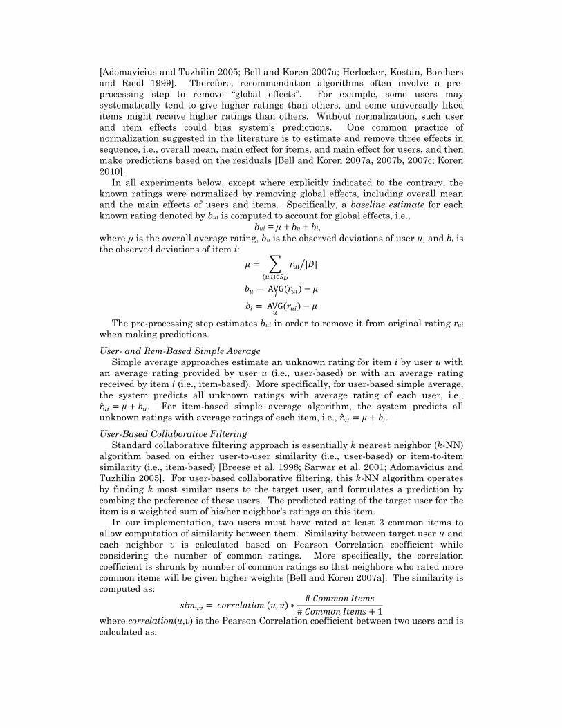
Experimental results on all datasets are summarized in Table 3, where, for the sake of completeness, we provide accuracy and stability numbers both as measured by the mean absolute error and shift (MAE and MAS) as well as the root mean squared error and shift (RMSE and RMSS). However, we note that both sets of measures were highly consistent with each other throughout our experiments, therefore, we will use only RMSE and RMSS measures in the remainder of the paper. Also Figure 6 provides a visual performance illustration of an average (of five runs) accuracy and stability performance (measured in RMSE and RMSS) of all algorithms on Netflix dataset using accuracy-stability plot. The horizontal axis represents accuracy and vertical axis stability. Numeric values on axes are arranged in reverse order of RMSE and RMSS, therefore, techniques located in the bottom left corner are the least accurate and least stable, while techniques in the top right corner are the most accurate and most stable.

Predictably, for all datasets, the more sophisticated recommendation algorithms (such as SVD, CF_Item, and CF_User) demonstrated better predictive accuracy than much simpler average-based techniques. In terms of stability, as expected, both user-based and item-based averages had prediction shift values of zero, i.e., adding new ratings that are identical to the current item (or user) average does not change the item (or user) average, thus, leaving the original predictions made using the simple average heuristics unaffected. In other words, user-based and item-based averages are perfectly stable due to their sum-of-squares-minimizing nature, as discussed in Section 2. Both CF_User and CF_Item regularly demonstrated a high level of instability; for example, RMSS for these techniques was 0.471 and 0.454, respectively, on the Netflix dataset. This is a significant shift in prediction, considering the length of the rating scale for this dataset is 4.0 (i.e., ratings go from 1

to 5). For datasets that have comparable total numbers of users and items (which is a proxy of the size of pool for identifying similar neighbors), CF_Item also exhibited higher stability than CF_User. The only exception took place in Jester data in which the number of users is more than 70 times of the number of items. Furthermore, while SVD demonstrated slightly higher or comparable predictive accuracy than CF_Item and CF_User, this model-based matrix factorization (SVD) technique, which is based on the global optimization approach, exhibited much higher stability than the memory-based neighborhood techniques (CF_Item and CF_User) that are based on the “local”, nearest neighbor heuristics. For example, RMSS for SVD were only 0.116, 0.12, and 0.1 on Netflix, Movielens 100K, and 1M datasets (with rating scale of length 4), respectively, and 0.354 on the Jester dataset (with rating scale of length 20). In addition, the baseline approach (User_Item_Avg) demonstrated comparable level of stability to SVD, but its accuracy typically was lower than the accuracy of the more sophisticated algorithms (SVD, CF_User, and CF_Item).

Table 3. Accuracy and stability of recommendation algorithms.

Dataset Recommendation algorithm

Accuracy Stability RMS Error MA Error RMS Shift MA Shift

Movielens 100K (scale: 1~5)

SVD 0.939 0.739 0.120 0.089 CF_User 0.954 0.749 0.389 0.269 CF_Item 0.934 0.733 0.292 0.195 User_Avg 1.041 0.834 0 0 Item_Avg 1.022 0.815 0 0 User_Item_Avg 0.965 0.757 0.107 0.086

Movielens 1M (scale: 1~5)


Netflix (scale: 1~5)


Jester (scale: -10 ~10)


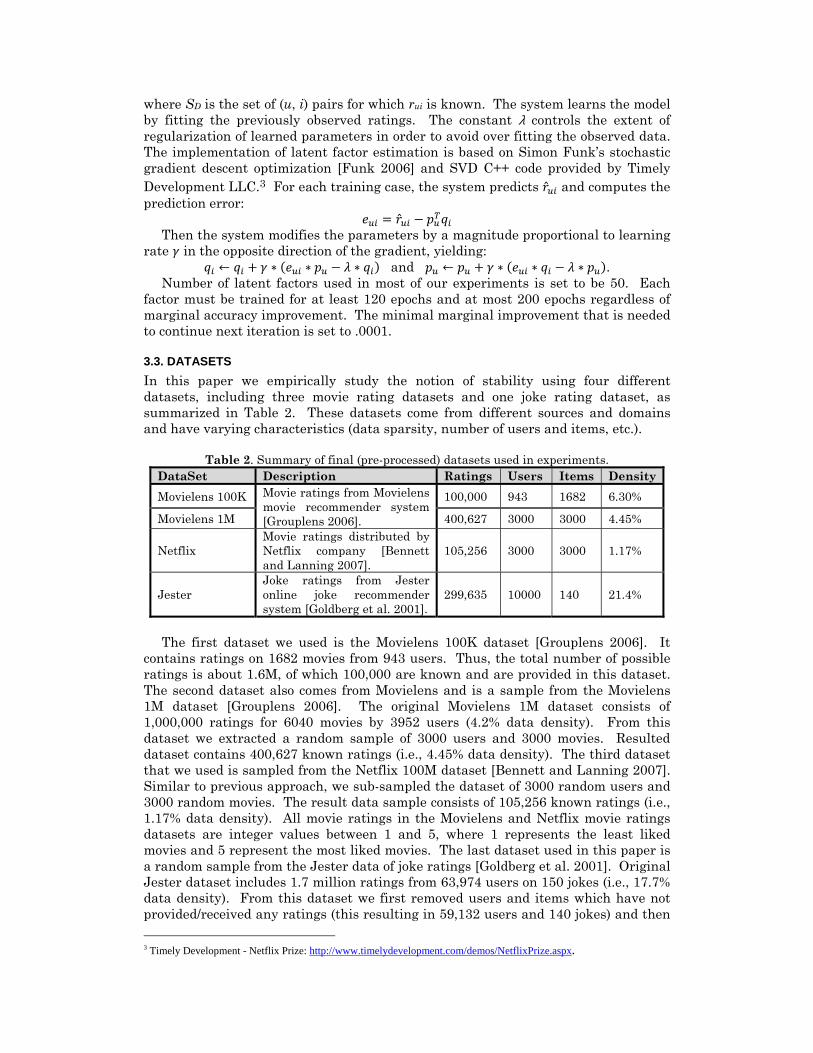
Figure 7 illustrates accuracy-stability plots of all five runs on four datasets. From

Figure 7, it can be seen that the variances of experiment results of five runs for all algorithms are relatively small. This is especially true for stability, suggesting that the stability performance of different recommendation techniques can be largely attributed to inherent characteristics of the algorithms rather than data variation in the random samples. Figure 7 also shows that stability of a recommendation algorithm does not necessarily correlate with its predictive accuracy. Recommendation algorithms can be relatively accurate but not stable (e.g., user- and item-based collaborative filtering approaches), or stable but not accurate (e.g., simple user average and item average heuristics), or both (e.g., matrix factorization approach), or neither (e.g., random guess heuristics would fit in this category).

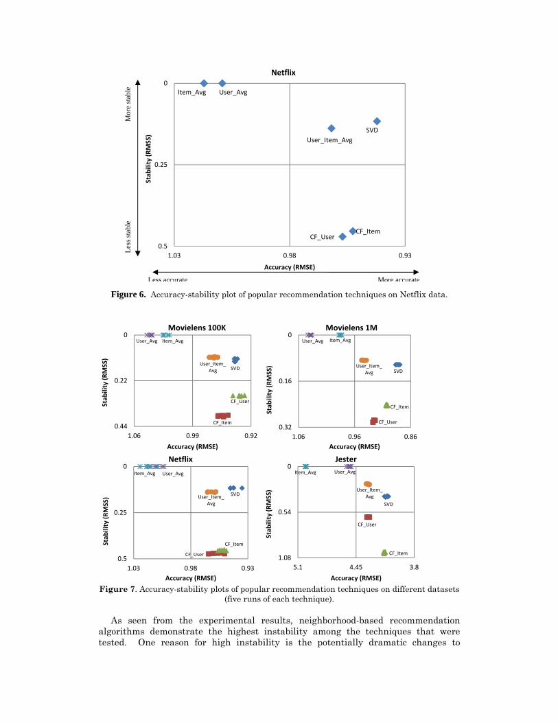
Figure 6. Accuracy-stability plot of popular recommendation techniques on Netflix data.

Figure 7. Accuracy-stability plots of popular recommendation techniques on different datasets

(five runs of each technique). As seen from the experimental results, neighborhood-based recommendation

algorithms demonstrate the highest instability among the techniques that were tested. One reason for high instability is the potentially dramatic changes to

SVD

CF_UserCF_Item

User_AvgItem_Avg

User_Item_Avg

0

0.25

0.50.930.981.03

Stab

ility (R

MSS)

Accuracy (RMSE)

Netflix

CF_User

SVD

CF_Item

User_Item_Avg

Item_AvgUser_Avg0

0.22

0.440.920.991.06

Stab

ility (R

MSS)

Accuracy (RMSE)

Movielens 100K

SVD

CF_Item

User_Item_Avg

Item_AvgUser_Avg

CF_User

0

0.16

0.320.860.961.06

Stab

ility (R

MSS)

Accuracy (RMSE)

Movielens 1M

CF_User

Item_Avg

SVDUser_Item_Avg

CF_Item

User_Avg0

0.25

0.50.930.981.03

Stab

ility (R

MSS)

Accuracy (RMSE)

Netflix

CF_User

SVD

CF_Item

User_Item_Avg

Item_Avg User_Avg0

0.54

1.083.84.455.1

Stab

ility (R

MSS)

Accuracy (RMSE)

Jester

Less

stab

le

Mor

e st

able

More accurateLess accurate

neighborhoods re-estimation when new ratings are added. To illustrate this, Figure 8 gives a simple numeric example that follows the scenario described in Section 1 (see Figure 1). Assume that we have five users and seven items, and the recommender system uses the simple variation of the traditional user-based collaborative filtering approach to make predictions for target users based on two nearest neighbors who share similar personal tastes in movies. As Figure 8 indicates, the system initially knows Alice’s ratings only for items 1, 2, 3, but not for items 4, 5, 6 and 7. At that time, the system indicates that users Bob and Carol are two nearest neighbors of Alice, as both of them provided the same exact ratings to common items (i.e., items 1, 2, and 3). Therefore, Alice’s ratings on items 4-7 are predicted to be the average of Bob and Carol’s ratings on these items, i.e., Alice is predicted to rate items 4-7 as 4, 4, 5, and 1, respectively. Then, following our earlier scenario, let’s assume that Alice has consumed recommended items 4-6 and submitted ratings on these items that were exactly the same as the system’s predictions. With the new incoming ratings, the system now finds the most similar users for Alice to be Dave and Eve, because they rated all common items exactly the same. Following the same user-based collaborative filtering approach, the prediction for Alice’s rating on item 7 is the average of Dave and Eve’s ratings on this item. Thus, the predicted rating for Alice on item 7 changes from 1 to 5 (from the least liked to most liked). The two contradictory predicted ratings on item 7 for Alice can be attributed to the dramatic change in the neighborhood that the system’s determined for Alice. With the small neighborhood size used for making predictions (i.e., k = 2), new addition of incoming ratings completely changed Alice’s neighborhood.

Stage 1

Alice 4 2 1 ? ? ? ? Bob 4 2 1 3 5 5 1

Carol 4 2 1 5 3 5 1

Dave 4 ? ? 4 4 5 5

Eve ? 2 ? 4 4 5 5

Stage 2

Alice 4 2 1 4 4 5 ? Bob 4 2 1 3 5 5 1

Carol 4 2 1 5 3 5 1

Dave 4 ? ? 4 4 5 5

Eve ? 2 ? 4 4 5 5 Figure 8. Instability of neighborhood-based recommendation algorithms: a numeric example.

In previous experiments, we used ratings given/received by 50 neighbors to make

predictions for each user/item. We also used 50 latent factors to represent each user and item in SVD implementation. In this section, we varied these algorithmic parameters to explore their influence on stability of these recommendation algorithms. More specifically, the size of neighborhood (i.e., denoted by k) used in neighborhood-based algorithms was varied from 1 to 100, and number of latent factors used to represent each user and item in matrix factorization (i.e., SVD) was also varied from 1 to 100. Prior studies have established that size of neighborhood and number of latent factors have some impact on predictive accuracy. We design a set of experiments to examine if stability is influenced by these algorithmic

parameters. Figure 9 illustrates the accuracy-stability plots for all four datasets. Increasing

number of neighbors and number of latent variables can significantly improve both accuracy and stability. When only a small number of neighbors are used to make predictions, adding new incoming ratings can change the neighborhood dramatically and, therefore, change the predicted ratings significantly. On the other hand, large neighborhood is more robust to additions of new incoming ratings, and hence leads to higher stability in future predictions. However, increasing number of latent factors did not seem to have significant impact on stability of SVD. In other words, neighborhood-based techniques are much more susceptible to changes in algorithmic parameters.

Figure 9 also shows that, for all datasets, the increment in both stability and accuracy by increasing size of neighborhood become subtle after going beyond 50 neighbors. Therefore, in the remainder of this paper, 50 neighbors were used for neighborhood-based techniques, i.e., the ratings provided by 50 most similar users for CF_User or received by 50 most similar items for CF_Item were used to compute predictions. Meanwhile, the number of latent variables used in SVD did not have significant impact for SVD. However, to be consistent and comparable across parameter settings, throughout the paper 50 latent variables were used in all SVD experiments to represent each user and item. In summary, all following experiments are based on the setting of 50 neigbhors for CF_User and CF_Item and 50 latent variables for SVD.

Figure 9. Stability of recommendation techniques for different neighborhood sizes and different numbers of latent factors.

4.2. IMPACT OF DATA SPARSITY Data sparsity is often cited as one of the reasons for inadequate recommender systems accuracy [Adomavicius and Tuzhilin 2005; Balabanovic and Shoham 1997; Billsus and Pazzani 1998; Breese et al. 1998; Sarwar et al. 1998]. In this section we

K=1

K=2K=3

K=5K=10 K=50

K=100

K=20

0

0.3

0.6

0.9

1.2

1.50.911.11.21.3

Stab

ility (R

MSS)

Accuracy (RMSE)

Movielens 100K

K=1

K=2K=3

K=5K=10

K=20K=50K=100

0

0.3

0.6

0.9

1.2

1.50.811.21.4

Stab

ility (R

MSS)

Accuracy (RMSE)

Movielens 1M

K=1

K=2K=3

K=10K=5 K=50

K=20

K=100

0

0.2

0.4

0.6

0.8

1

1.20.911.11.21.3

Stab

ility (R

MSS)

Accuracy (RMSE)

Netflix

K=1

K=2

K=3K=5K=10

K=20K=50K=100

0

1

2

3

4

5

644.555.56

Stab

ility (R

MSS)

Accuracy (RMSE)

Jester

perform an empirical investigation on whether data sparsity (or density) has an impact on the stability as well, by observing the stability and accuracy of recommendation algorithms at different data density levels. Density of the four datasets used for our original experiments is 6.3%, 4.45%, 1.17%, and 21.4%, respectively, and to manipulate these density levels, we draw random samples from the original datasets that contained 30%, 40%, 50%, …, 90% of ratings, thus, obtaining rating data subsamples with wide-ranging density. Also, because only subsets of actual ratings in the dataset were used for training, we were able to use the rest of the data as part of the predictive accuracy evaluation.

Graphs on the left side in Figure 10 show the comparisons of accuracy of recommendation algorithms with varied levels of data density. Our results are consistent with prior literature in that the recommendation algorithms typically demonstrate higher predictive accuracy on denser rating datasets. More importantly, graphs on the right in Figure 10 show that the density level of the rating data also has a significant influence on recommendation stability for the neighborhood-based CF techniques (CF_Item and CF_User) – RMSS increases as the rating data becomes sparser. In other words, as data becomes sparser, these techniques are increasingly more sensitive to additions of new ratings (even though they are in complete agreement with the algorithms’ own predictions). In particular, in our sparsest samples (0.351% rating density, sampled from Netflix), both CF_User and CF_Item demonstrate a very significant 0.57 RMSS (on the rating scale from 1 to 5). Meanwhile, the stability performance of the model-based matrix factorization (SVD) as well as the baseline (User_Item_Avg) approaches is much more advantageous and more consistent across different density levels, consistently staying in the 0.1-0.15 RMSS range for the movie rating datasets (with the 1-5 rating scale) and in the 0.3-0.4 RMSS range for the Jester dataset (with the scale from -10 to +10). In summary, the experimental results show that the stability of the model-based approaches (SVD, User_Item_Avg, User_Avg, Item_Avg) is robust to data density changes, in contrast to the neighborhood-based collaborative filtering heuristics.

4.3. IMPACT OF NUMBER OF NEW RATINGS ADDED

In order to further understand the dynamics of recommendation stability, in the next set of experiments we varied the number of new incoming ratings (that are in complete agreement with the system’s prior predictions). Note that these experiments can be thought of as simulating the length of the time period over which the stability is being measured. More and more ratings are made available to the system as time passes by, thus, longer time period is associated with more incoming ratings. The number of new ratings (to be added to the existing set of known ratings) ranged from 10% to 500% of the size of known ratings, and these ratings were randomly drawn from all the available predicted ratings. Figure 11 shows the dynamics of recommendation stability (as measured by RMSS) for different numbers of new ratings.

In particular, as expected, we find that the prediction shift for the simple user- and item-average approaches is always zero, regardless of how many predictions were added to rating matrix. For all other techniques, including the matrix factorization (SVD), user- and item-based collaborative filtering (CF_User and CF_Item), and baseline estimates using user and item averages (User_Item_Avg), the prediction shift curves generally indicate a convex shape. In particular, with only very few newly introduced ratings the prediction shift is small, but the instability rises very rapidly until the number of newly introduced ratings reaches about 20% of the original data, at which point the rise of the prediction shift slows down and later starts exhibiting a slow continuous decrease.

Figure 10. Comparison of accuracy and stability of recommendation techniques for different data density levels.

Our experiments suggest that the stability of memory-based neighborhood

techniques is more sensitive to the number of new incoming ratings than the stability

0.9

0.93

0.96

0.99

1.02

1.05

1.08

1.5 3.5 5.5

RMS Error

Rating Data Density (%)

Movielens 100K

0

0.1

0.2

0.3

0.4

0.5

0.6

1.5 2.5 3.5 4.5 5.5

RMS Shift


Movielens 100K

0.85

0.9

0.95

1

1.05

1.1

1 2 3 4

RMS Error


Movielens 1M

0

0.1

0.2

0.3

0.4

0.5

1 2 3 4

RMS Shift


Movielens 1M

0.92

0.94

0.96

0.98

1

1.02

1.04

1.06

0.3 0.6 0.9 1.2

RMS Error


Netflix

0

0.1

0.2

0.3

0.4

0.5

0.6

0.3 0.6 0.9 1.2

RMS Shift


Netflix

4

4.2

4.4

4.6

4.8

5

5.2

6 11 16 21

RMS Error


Jester

0

0.3

0.6

0.9

1.2

1.5

6 11 16 21

RMS Shift


Jester

of model-based techniques that are based on global optimization approaches (including both matrix factorization and simpler average-based models). When only a very small number of new ratings is added, the original rating patterns persist in the data and the neighborhood of each user (or item) does not change dramatically, resulting in similar predictions for the same items (i.e., higher stability). In contrast, when more and more new ratings are made available, the neighborhoods can be affected very dramatically. This is supported by the observed more rapid decrease of stability in neighborhood-based techniques as compared to the model-based approaches, which are based on global optimization and, thus, are less malleable to additions of new ratings (that are in agreement of what the algorithm had predicted earlier).

In addition, it is important to note that, after the initial increase in prediction shift, its subsequent slow decrease (for all recommendation algorithms) can be attributed to the sheer numbers of additional new ratings that are introduced, all of which are in agreement with the initial recommendation model. Whether the recommendation algorithm is more computationally sophisticated (e.g., SVD) or less (e.g., CF_User), providing it with increasingly more data that is in consistent agreement with some specific model will make this algorithm represent this model better and make more accurate and more stable recommendations.

Figure 11. Stability of recommendation techniques for varying numbers of incoming ratings.

4.4. IMPACT OF NEW RATING DISTRIBUTION

We also varied the sampling strategy that was used to select the new incoming ratings. The objective was to test the impact of the incoming rating distribution on the stability of recommendation algorithms. We applied five different sampling strategies to draw samples of the same sizes (i.e., 100K, 400K, 105K and 300K, respectively, for the four datasets described in Table 2) as the original rating data

0

0.1

0.2

0.3

0.4

0 2 4

RMS Shift

Size of Incoming Ratingsx 100000

Movielens 100K

0

0.05

0.1

0.15

0.2

0.25

0.3

0 1 2

RMS Shift

Size of Incoming Ratings Millions

Movielens 1M

0

0.1

0.2

0.3

0.4

0.5

0 2 4

RMS Shfit

Size of Incoming Ratings x 100000

Netflix

0

0.2

0.4

0.6

0.8

1

1.2

0 5 10

RMS Shift

Size of Incoming Ratings x 100000

Jester

from all the available system’s predicted ratings: Random, High, HighHalf, Low, and LowHalf.

Random strategy draws a sample of predictions from each user at random to be added as new incoming ratings to the set of original ratings (i.e., corresponding to the situation where the users will choose to watch new movies at random); High strategy sorts all predictions for each user and only chooses those with highest predicted rating values (i.e., in this scenario the users will exactly follow the recommendation algorithm to choose movies and highest ratings are the ones that will be added to the system); HighHalf sorts predictions for each user and then draws a random sample of predictions with values greater than the median prediction (i.e., users will follow the recommender algorithm to separate good movies from the bad, but then will choose among the good movies at random); Low sorts predictions for each user and only adds lowest predictions (i.e., opposite of High; included here for completeness); and LowHalf sorts predictions and draws a random sample from ratings whose values are lower than the median prediction (i.e., opposite of HighHalf; included for completeness). The five strategies are summarized in Table 4. In summary, we wanted to test whether adding skewed rating samples (e.g., high ratings only or low ratings only) will bias the original rating distribution and, as a result, decrease recommendation algorithm stability, as compared to the random samples of new predictions.

Table 4. Summary of sampling strategies for new rating selection.

Strategy

Details

Random Randomly add a sample of predicted ratings to existing known ratings High Add highest predicted ratings (e.g., 5) to existing known ratings HighHalf Add a random sample of predicted ratings with values above median

prediction Low Add lowest predicted ratings (e.g., 1) to existing known ratings LowHalf Add a random sample of predicted ratings with values below median

prediction Comparison of recommendation algorithms in terms of their stability for different

incoming rating distributions is presented in Figure 12. As can be seen from the figure, the distribution of new incoming ratings significantly influences the stability of recommendation algorithms, except for simple user- and item-based average techniques, which are always perfectly stable, as discussed earlier. In particular, among the five sampling strategies, Random strategy demonstrated the highest stability for nearly all recommendation algorithms. Moreover, all recommendation algorithms exhibited an increase in instability with High or Low sampling strategies, as compared to the Random strategy, and this difference was especially substantial for memory-based neighborhood CF techniques (CF_User and CF_Item). For example, the prediction shift of user-based CF method rises from about 0.45 with Random strategy all the way to about 1.0 with Low strategy on Netflix dataset (on the scale of length 4, i.e., from 1 to 5). Furthermore, adding new ratings selected by HighHalf and LowHalf strategies led to moderate prediction shift for all algorithms. In summary, Random rating samples that are in complete agreement with previous predictions have more favorable impact on stability than samples with skewed distribution.

Figure 12 also shows that the stability patterns obtained using all datasets are essentially consistent. More specifically, the more skewed the distribution of new incoming ratings is, the less stable the recommendation algorithms become. In addition, model-based approaches (including matrix factorization and simple average estimates) continue to be substantially more stable than neighborhood-based

heuristics.

Figure 12. Stability of recommendation techniques with varied distributions of added ratings.

Figure 13. Difference in mean ratings for User_Item_Avg for different sampling strategies on

Movielens 100K dataset.

Our results also suggest that the impact of adding skewed samples of new ratings on recommendation stability can be asymmetric for some algorithms on some datasets, e.g., User_Item_Avg had the best stability using HighHalf strategy (and not Random strategy, like many other techniques) on Movielens 100K, Movielens 1M, and Netflix datasets. One explanation for this phenomenon is that the original ratings data is skewed toward high ratings. For example, in Movielens 100K dataset, the mean of ratings in the original data is 3.5 (on a scale 1 to 5). Because of this, among the five sampling strategies, the HighHalf strategy used with User_Item_Avg algorithm provided the ratings that turned out to have the distribution that was the most similar to the distribution of the original data and,

0

0.2

0.4

0.6

0.8

1

Low LowHalf Random HighHalf High

RMS Shift

Movielens 100K

0

0.2

0.4

0.6

0.8


RMS Shift

Movielens 1M

0

0.2

0.4

0.6

0.8

1

1.2


RMS Shift

Netflix

0

0.5

1

1.5

2

2.5


RMS Shift

Jester

0.0

0.3

0.6

0.9

1.2


Mean Ra

ting

Differen

ce

Movielens 100K

Avg(Original+New)‐Avg(Original)

therefore, introduced least prediction shift. This is illustrated in Figure 13, which presents the difference between rating means in the original 100K dataset and the data resulting from all five sampling strategies for the User_Item_Avg technique.

4.5. IMPACT OF DATA NORMALIZATION In all previous experiments, before applying collaborative filtering approaches or matrix factorization method, the rating data was normalized by removing “global effects” (including the overall mean, user average, and item average) in the way that is often used in recommender systems literature [Bell and Koren 2007a]. In this section, we investigate the impact of data normalization on the stability of recommendation algorithms. Figure 14 summarizes our findings. In particular, we implemented two versions of matrix factorization (SVD) algorithm, with normalization (i.e., removing the baseline) and without. For the two neighborhood-based approaches (CF_User and CF_Item), we implemented three versions of each: with normalization by removing the baseline, with normalization by removing the user average for CF_User or item average for CF_Item, and without normalization. Simple average heuristics essentially represent the normalization procedures and, thus, we only have a single version of each.

Figure 14. Stability of recommendation techniques with and without data normalization.

The results suggest that normalizing rating data in general can improve predictive accuracy for all recommendation algorithms. Meanwhile, normalization also impacts the stability of these algorithms in different ways. For example, normalizing data by removing baseline estimate slightly reduced the stability of matrix factorization algorithm as compared to no normalization. However, normalization by removing just the item average or user average dramatically improved both accuracy and stability of neighborhood-based approaches as compared

SVD

CF_User

CF_Item

CF_USer

CF_Item

SVD

CF_User

CF_Item

Item_AvgUser_Avg

User_Item_Avg

0

0.47

0.940.881.031.18

Stab

ility (R

MSS)

Accuracy (RMSE)

Movielens 100K

SVD

CF_UserCF_Item

CF_USer

CF_Item SVD

CF_User

CF_Item

Item_AvgUser_Avg

User_Item_Avg

0

0.45

0.90.840.971.1

Stab

ility (R

MSS)

Accuracy (RMSE)

Movielens 1M

SVD

CF_UserCF_Item

CF_USerCF_Item

SVD

CF_User

CF_Item

Item_Avg User_Avg

User_Item_Avg

0

0.8

1.60.91.151.4

Stab

ility (R

MSS)

Accuracy (RMSE)

Netflix

SVD

CF_User

CF_Item

CF_USer

CF_Item

SVD

CF_UserCF_Item

Item_Avg User_Avg

User_Item_Avg

0

0.75

1.53.94.55.1

Stab

ility (R

MSS)

Accuracy (RMSE)

Jester

to their non-normalized versions. On top of this, removing all the global effects (i.e., baseline estimate) resulted in a comparable accuracy and only very slight stability improvement, as compared to removing only one main effect (i.e., user average or item average). Moreover, the impacts of normalization on stability and accuracy are consistent across all datasets.

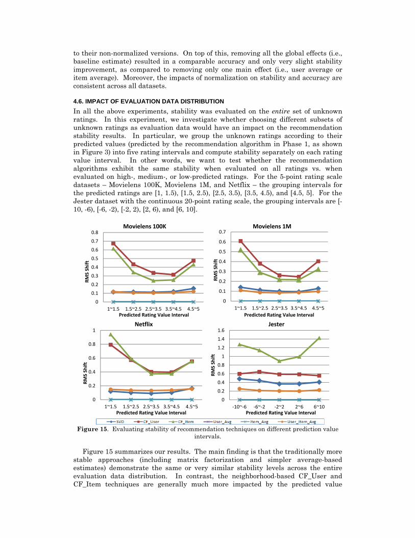
4.6. IMPACT OF EVALUATION DATA DISTRIBUTION In all the above experiments, stability was evaluated on the entire set of unknown ratings. In this experiment, we investigate whether choosing different subsets of unknown ratings as evaluation data would have an impact on the recommendation stability results. In particular, we group the unknown ratings according to their predicted values (predicted by the recommendation algorithm in Phase 1, as shown in Figure 3) into five rating intervals and compute stability separately on each rating value interval. In other words, we want to test whether the recommendation algorithms exhibit the same stability when evaluated on all ratings vs. when evaluated on high-, medium-, or low-predicted ratings. For the 5-point rating scale datasets – Movielens 100K, Movielens 1M, and Netflix – the grouping intervals for the predicted ratings are [1, 1.5), [1.5, 2.5), [2.5, 3.5), [3.5, 4.5), and [4.5, 5]. For the Jester dataset with the continuous 20-point rating scale, the grouping intervals are [-10, -6), [-6, -2), [-2, 2), [2, 6), and [6, 10].

Figure 15. Evaluating stability of recommendation techniques on different prediction value intervals.

Figure 15 summarizes our results. The main finding is that the traditionally more

stable approaches (including matrix factorization and simpler average-based estimates) demonstrate the same or very similar stability levels across the entire evaluation data distribution. In contrast, the neighborhood-based CF_User and CF_Item techniques are generally much more impacted by the predicted value

0

0.1

0.2

0.3

0.4

0.5

0.6

0.7

0.8

1~1.5 1.5~2.5 2.5~3.5 3.5~4.5 4.5~5

RMS Shift

Predicted Rating Value Interval

Movielens 100K

0

0.1

0.2

0.3

0.4

0.5

0.6

0.7

1~1.5 1.5~2.5 2.5~3.5 3.5~4.5 4.5~5

RMS Shift


Movielens 1M

0

0.2

0.4

0.6

0.8

1

1~1.5 1.5~2.5 2.5~3.5 3.5~4.5 4.5~5

RMS Shift


Netflix

0

0.2

0.4

0.6

0.8

1

1.2

1.4

1.6

‐10~‐6 ‐6~‐2 ‐2~2 2~6 6~10

RMS Shift


Jester

distribution of the unknown ratings used for evaluation. Specifically, the predictions provided by neighborhood-based approaches are much less stable for the more extreme rating values (high or low) than for medium/neutral rating values. Furthermore, these patterns are highly consistent across different datasets.

5. RELATED WORK The notions of “stability” have appeared in many fields. Each field typically has its own definition(s) of stability, and these definitions may often refer to very different phenomena. For example, in mathematics alone one can find a number of different definitions of stability. In the dynamical systems subfield there are notions of structural stability and Lyapunov stability. Structural stability refers to the property of a dynamical system that the quantitative behavior of the trajectory is not affected by small perturbations of the system itself [Simitses and Hodges 2005]. Lyapunov stability considers perturbation of initial conditions for a fixed system and occurs when all solutions of the system converge to an equilibrium point [Lyapunov 1992]. Meanwhile, in the subfield of numerical analysis, numerical stability captures the property of an algorithm with respect to the round-off or truncation computation errors when performed on digital computers in practice [Burden and Faires 2004; Higham 2002]. Depending on specific computational method, small round-off or truncation errors can be damped out, or can be magnified and lead to much larger errors. Therefore, it is important for numerical analysts to identify numeric computation algorithms that are robust, i.e., that have good numerical stability among other desirable properties.

We find that many of the available definitions of stability are not directly related to the concept that we explore in this paper. Below we discuss the two notions that are somewhat related to our work, and which come from the areas of machine learning and attack detection in recommender systems.

Subsample-based stability of classification models. In the machine learning literature, the stability of a predictive algorithm is the degree to which it generates repeatable results, given different subsamples of the entire dataset [Turney 1994, 1995]. An algorithm is stable if it induces approximately the same model from two samples with the same probability distribution. Prior research has focused on the stability of binary classifiers (in particular, decision trees), and described a method to quantify stability based on the expected agreement between predictions from two different samples [Turney 1994, 1995]. More specifically, let D1 and D2 be two independent random sub samples of same size drawn from dataset D, and , and

, represent the models built using some learning algorithm T on samples D1 and D2, respectively. The stability of T is then defined to be the expected agreement between predictions on common unknown ratings made by two models, i.e.,

, ,

where , , is the probability that two predictions made on the same input x are of the same value.

Turney’s definition of stability essentially measures how robust a predictive algorithm is in detecting underlying patterns from random subsamples of the same dataset. In his own words, Turney describes that “[t]he instability of the algorithm is the sensitivity of the algorithm to noise in the data. Instability is closely related to our intuitive notion of complexity. Complex models tend to be unstable and simple models tend to be stable.” [Turney 1994] In contrast, the stability that we are interested in reflects not the representativeness of the random subsamples of original data or the strength of the underlying patterns in the original dataset with respect to a given learning technique, but rather reflects the inherent characteristics of this

learning technique, specifically, how internally (in)consistent the predictions made by this technique are.

Attack detection in recommender systems. Because recommender systems depend heavily on input from users, they are subject to manipulations and attacks [Lam and Riedl 2004; Massa and Bhattacharjee 2004; Mobasher et al. 2007; Mobasher et al. 2006a; Mobasher et al. 2006b; O’Mahony et al. 2004]. In this literature, the vulnerabilities of recommender systems are studied in terms of the robustness of such systems in the face of malicious attacks and are evaluated using a variety of metrics including robustness, stability, percentage of attack profiles, hit ratio, and average rank [Mobasher et al. 2007; O’Mahony et al. 2004]. Among them, the two commonly used metrics are robustness and stability. Robustness measures the performance of the system before and after an attack (e.g., difference in predictive accuracy). Stability looks at the shift in system’s predictions for the attacked items. Stability is often measured as the average prediction shift, which is a metric that corresponds to the MAS metric mentioned in this paper. However, in the recommendation system attack detection literature, stability of a recommender system measures the dynamics in system’s predictions when facing attacks from outside. In contrast, in this paper, we measure a very different aspect of stability (which can also be thought of as internal consistency) which represents not a consequence of an external force that deliberately attempts to manipulate the recommender system for some purpose, but a consequence of the algorithm’s own inherent inconsistencies.

6. CONCLUSIONS

In this paper, we introduce and investigate the notion of stability of recommendation algorithms. As discussed earlier, stability measures the extent to which a recommendation algorithm provides predictions that are consistent with each other; in stable algorithms, assuming that one prediction is perfectly accurate and, consequently, adding this prediction value to the algorithm’s training data would not invalidate or change other predictions. Another way to think about stability is that stable algorithms provide consistent predictions over time, assuming that new incoming ratings available to system are in complete agreement with system’s prior predictions. We believe that the stability should be a desired property for recommender systems designers, because it represents the internal consistency of a recommendation algorithm (as measured by the potential impact of algorithm’s predictions on its own future performance). We advocate that stability is an important dimension for measuring recommender systems performance; providing unstable, contradictory predictions could negatively affect the users’ confidence and trust in the system.

Aside from the development of the recommendation stability metric, this paper investigates the stability performance of six popular recommendation algorithms. In particular, we conducted extensive experiments using these algorithms on four different real-world datasets. The results of our experiments show that model-based techniques (e.g., matrix factorization, user average, item average, and baseline estimates using combined user and item averages) are regularly more stable, i.e., more consistent in their predictions, than memory-based collaborative filtering heuristics in a wide variety of settings. We also find that normalizing rating data before applying any algorithms not only improves accuracy for all recommendation algorithms, but also plays a critical role in improving their stability. More generally, we perform a comprehensive empirical analysis of many important factors (e.g., the sparsity of original rating data, the number of new incoming ratings, the distribution of incoming ratings, the distribution of evaluation data, etc.) and report the impact they have on the stability of the recommender system.

We also empirically show that stability of a recommendation algorithm does not necessarily correlate with its predictive accuracy. Recommendation algorithms can be relatively accurate but not stable (e.g., user- and item-based collaborative filtering approaches), or stable but not accurate (e.g., simple user average and item average heuristics), or both (e.g., matrix factorization approach), or neither (e.g., random guess heuristics).

This research also provides opportunities for some interesting and important research directions. In particular, in this paper we show that several widely popular recommendation algorithms (such as neighborhood-based collaborative filtering techniques) do not exhibit a high degree of stability in many data settings. Therefore, developing stability-aware or stability-maximizing recommendation techniques represents an interesting direction for future work. In summary, we believe that addressing the issue of recommendation stability deserves our attention and exploration in both research and practice. This paper represents just the first step in studying stability-related issues in recommender systems, and significant additional work is needed to explore this issue in a more comprehensive manner.

ACKNOWLEDGMENTS This work was supported in part by the National Science Foundation grant IIS-0546443.

REFERENCES ADOMAVICIUS, G. and TUZHILIN, A. 2005. Toward the Next Generation of Recommendation System: A

Survey of the State-of-the-Art and Possible Extensions. IEEE Transactions on Knowledge and Data Engineering 17, 734-749.

ADOMAVICIUS, G. and ZHANG, J. 2010. On the Stability of Recommendation Algorithms. In ACM Conference on Recommender systems, New York, Barcelona, Spain, 47-54.

BALABANOVIC, M. AND SHOHAM, Y. 1997. Fab: Content-based, collaborative recommendation. Communications of the ACM. 40, 3, 66–72.

BELL, R.M. and KOREN, Y. 2007a. Improved Neighborhood-based Collaborative Filtering. In KDD Cup'07, San Jose, CA, USA, 7-14.

BELL, R.M. and KOREN, Y. 2007b. Lessons from the Netflix prize challenge. ACM SIGKDD Explorations Newsletter 9, 75-79.

BELL, R.M. and KOREN, Y. 2007c. Scalable Collaborative Filtering with Jointly Derived Neighborhood Interpolation Weights In Seventh IEEE International Conference on Data Mining, Omaha, NE, USA.

BENNETT, J. and LANNING, S. 2007. The Netflix Prize. In KDD-Cup and Workshop, San Jose, CA, www.netflixprize.com.

BILLSUS, D. AND PAZZANI, M. 1998. Learning collaborative information Filters. In the Fifteenth International Conference on Machine Learning (ICML '98). 46-54.

BREESE, J.S., HECKERMAN, D. and KADIE, C. 1998. Empirical analysis of predictive algorithms for collaborative filtering. In Fourteenth Conference on Uncertainty in Artificial Intelligence, Madison, WI.

BURDEN, R.L. and FAIRES, D. 2004. Numerical Analysis. Thomson Brooks/Cole, U.S. D’ASTOUS, A., and TOUIL, N. 1999. Consumer Evaluations of Movies on the Basis of Critics' Judgments.

Psychology & Marketing 16, 677–694. DIAS, M.B., LOCHER, D., LI, M., EL-DEREDY, W., and LISBOA, P. 2008. The value of personalised

recommender systems to e-business: a case study. In 2008 ACM conference on Recommender systems (RecSys '08). ACM, New York, NY, USA, 291-294. DOI=10.1145/1454008.1454054 http://doi.acm.org/10.1145/1454008.1454054.

DUDA, R.O., HART, P.E. and STORK, D.G. 2000. Pattern Classification. Wiley-Interscience. FUNK, S. 2006. Netflix Update: Try This at Home. In Netflix Update: Try This at Home. GARFINKEL, R., GOPAL, R., PATHAK, B., VENKATESAN, R. and YIN, F. 2006. Empirical Analysis of

the Business Value of Recommender Systems (November 2006). Available at SSRN: http://ssrn.com/abstract=958770.

GERSHOFF, A., MUKHERJEE, A., and MUKHOPADHYAY, A. 2003. Consumer Acceptance of Online Agent Advice: Extremity and Positivity Effects. Journal of Consumer Psychology 13:1&2, 161-170.

GOLDBERG, K., ROEDER, T., GUPTA, D. and PERKINS, C. 2001. Eigentaste: A Constant Time Collaborative Filtering Algorithm. Information Retrieval 4, 133-151.

GROUPLENS 2006. Movielens Data Sets. HASTIE, T., TIBSHIRANI, R. and FRIEDMAN, J. 2009. The Elements of Statistical Learning: Data

Mining, Inference, and Prediction. Springer. HERLOCKER, J., KOSTAN, J., BORCHERS, A. and RIEDL, J. 1999. An Algorithmic Framework for

Performing Collaborative Filtering. In 22nd ACM SIGIR Conference on Information Retrieval, 230-237.

HERLOCKER, J.L., KONSTAN, J.A., TERVEEN, K. and RIEDL, J.T. 2004. Evaluating collaborative filtering recommender systems. ACM Transactions on Information Systems 22, 5-53.

HIGHAM, N.J. 2002. Accuracy and Stability of Numerical Algorithms. SIAM: Society for Industrial and Applied Mathematics, Philadelphia.

KOMIAK, S. and BENBASAT, I. 2006. The effects of personalization and familiarity on trust and adoption of recommendation agents. MIS Quarterly 30, 941-960.

KOREN, Y. 2010. Factor in the Neighbors: Scalable and Accurate Collaborative Filtering. ACM Transactions on Knowledge Discovery from Data 4, 1-24.

KOREN, Y., BELL, R. and VOLINSKY, C. 2009. Matrix Factorization Techniques For Recommender Systems. IEEE Computer 42, 30-37.

KOSTAN, J., MILLER, B., MALTZ, D., HERLOCKER, J., GORDON, L. and RIEDL, J. 1997. GroupLens: Applying Collaborative Filtering to Usenet news. Communications of the ACM 40, 77-87.

LAM, S. and RIEDL, J. 2004. Shilling Recommender Systems for Fun and Profit. In the 13th international conference on World Wide Web New York City, NY.

LEGWINSKI, T. 2010. Recommendation Explanations Increase Sales & Customer Confidence. http://blog.strands.com/2010/03/17/recommendations-increase-sales-customer-confidence/

LYAPUNOV, A.M. 1992. The general problem of the stability of motion. CRC Press. MASSA, P. and AVESANI, P. 2006. Trust-aware Bootstrapping of Recommender Systems. In ECAI

Workshop on Recommender Systems. MASSA, P. and BHATTACHARJEE, B. 2004. Using trust in recommender systems: An experimental

analysis. In Trust Management, Proceeding Springer-Verlag Berlin, Berlin, 221-235. MOBASHER, B., BURKE, R., BHAUMIK, R. and WILLIAMS, C. 2007. Toward Trustworthy Recommender

Systems: An Analysis of Attack Models and Algorithm Robustness. ACM Transactions on Internet Technology 7, 23:21-23:38.

MOBASHER, B., BURKE, R. and SANDVIG, J.J. 2006a. Model-Based Collaborative Filtering as a Defense against Profile Injection Attacks. In 21st Conference on Artificial Intelligence (AAAI'06), Boston, MA.

MOBASHER, B., BURKE, R., WILLIAMS, C. and BHAUMIK, R. 2006b. Analysis and detection of segment-focused attacks against collaborative recommendation. In Advances in Web Mining and Web Usage Analysis Springer-Verlag Berlin, Berlin, 96-118.

O'DONOVAN, J. and SMYTH, B. 2006. Mining trust values from recommendation errors. International Journal on Artificial Intelligence Tools 15, 945-962.

O'MAHONY, M.P., HURLEY, N.J. and SILVESTRE, G.C.M. 2004. An evaluation of neighbourhood formation on the performance of collaborative filtering. Artificial Intelligence Review 21, 215-228.

O’DONOVAN, J. and SMYTH, B. 2005. Trust in recommender systems. In 10th international conference on Intelligent user interfaces, San Diego, California, USA.

RESNICK, P., IACOVOU, N., SUCHAK, M., BERGSTROM, P. and RIEDL, J. 1994. Grouplens: an open architecture for collaborative filtering of netnews. In Conference on Computer Supported Cooperative Work (CSCW94), 175–186.

RIGBY, C. 2011. Internet Retailing webinars. Review: Boosting email marketing revenue with personalised recommendations by Silverpop, Baynote and MusicRoom.com. http://www.internetretailing.net/2011/10/internet-retailing-webinars-review-boosting-email-marketing-revenue-with-personalised-recommendations-by-silverpop-baynote-and-musicroom-com/.

SARWAR, B., KARYPIS, G., KONSTAN, J.A. and RIEDL, J. 2001. Item-based Collaborative Filtering Recommendation Algorithms. In the 10th International WWW Conference, Hong Kong, 285 - 295.

SARWAR,B., KONSTAN, J., BORCHERS, A., HERLOCKER, J., MILLER, B. AND RIEDL, J. 1998. Using filtering agents to improve prediction quality in the Grouplens research collaborative filtering system. In ACM Conf. on Computer Supported Cooperative Work, 345–354. New York, NY, USA.

SHANI, G. and GUNAWARDANA, A. 2011. Evaluating Recommender Systems [book chapter]. In P. Kantor, F. Ricci, L. Rokach, B. Shapira (Eds.), Recommender Systems Handbook: A Complete Guide for Research Scientists and Practitioners, Springer, 2011.

SIMITSES, G. and HODGES, D. 2005. Fundamentals of Structural Stability. Butterworth-Heinemann, Burlington, MA.

TURNEY, P. 1994. A Theory of Cross-Validation Error. Journal of Experimental and Theoretical Artificial Intelligence 6, 361-391.

TURNEY, P. 1995. Technical Note: Bias and the Quantification of Stability. Machine Learning 20, 23-33. VAN SWOL, L.M., and SNIEZEK, J.A. 2005. Factors Affecting the Acceptance of Expert Advice. British

Journal of Social Psychology 44:3, 443-461. WANG, W. and BENBASAT, I. 2005. Trust in and adoption of online recommendation agents. Journal of

the Association for Information Systems 6, 72-101.

stability of collaborative filtering recommendation

Documents