stability - ptolemy projectin particular, let xˆ denote the laplace or z transform of x, depending...
TRANSCRIPT

Chapter 12
Stability
The four Fourier transforms prove to be useful tools for analyzing signals and systems. When asystem is LTI, it is characterized by its frequency response H , and its input x and output y arerelated simply by
∀ω∈ Reals, Y(ω) = H(ω)X(ω),
where Y is the Fourier transform of y, and X is the Fourier transform of x.
However, we ignored a lurking problem. Any of the three Fourier transforms, X, Y, or H , may notexist. Suppose for example that x is a discrete-time signal. Then its Fourier transform (the DTFT)is given by
∀ ω∈ Reals, X(ω) =∞
∑n=−∞
x(n)e−iωn. (12.1)
This is an infinite sum, properly viewed as the limit
∀ ω∈ Reals, X(ω) = limN→∞
N
∑n=−N
x(n)e−iωn. (12.2)
As with all such limits, there is a risk that it does not exist. If the limit does not exist for anyω∈ Reals, then the Fourier transform becomes mathematically treacherous at best (involving, forexample, Dirac delta functions), and mathematical nonsense at worst.
Example 12.1: Consider the sequence
x(n) ={
0, n≤ 0an−1, n > 0
,
where a > 1 is a constant. Plugging into (12.1), the Fourier transform should be
∀ ω∈ Reals, X(ω) =∞
∑n=0
an−1e−iωn.
At ω= 0, it is easy to see that this sum is infinite (every term in the sum is greater thanor equal to one). At other values of ω, there are also problems. For example, at ω= π,
393

394 CHAPTER 12. STABILITY
Mbody
tail
main rotor shaft
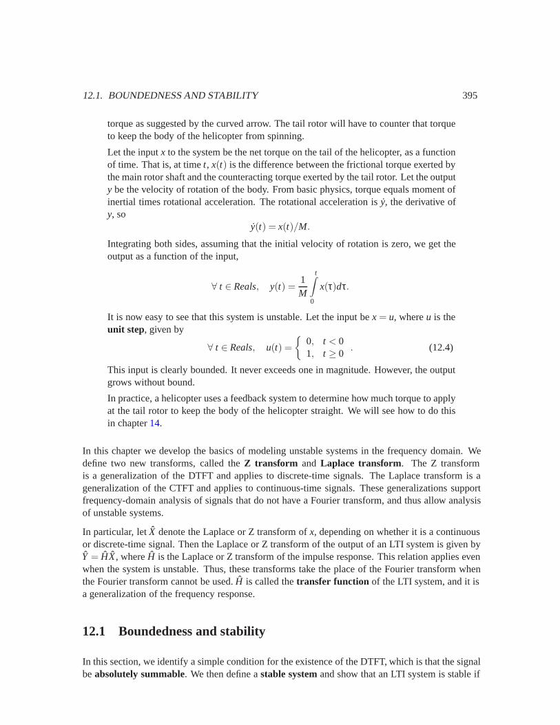
Figure 12.1: A highly simplified helicopter.
the terms of the sum alternate in sign and increase in magnitude as n gets larger. Thelimit (12.2) clearly will not exist.
A similar problem arises with continuous-time signals. If x is a continuous-time signal, then itsFourier transform (the CTFT) is given by
∀ ω∈Reals, X(ω) =∞∫−∞
x(t)e−iωtdt. (12.3)
Again, there is a risk that this integral does not exist.
This chapter studies signals for which the Fourier transform does not exist. Such signals prove to beboth common and useful. The signal in example 12.1 gives the bank balance of example 5.12 whenan initial deposit of one dollar is made, and no further deposits or withdrawals are made (thus, it isthe impulse response of the bank account). This signal grows without bound, and any signal thatgrows without bound will cause difficulties when using the Fourier transform.
The bank account is said to be an unstable system, because its output can grow without bound evenwhen the input is always bounded. Such unstable systems are common, so it is unfortunate that thefrequency domain methods we have studied so far do not appear to apply.
Example 12.2: A helicopter is intrinsically an unstable system, requiring an electronicor mechanical feedback control system to stabilize it. It has two rotors, one above,which provides lift, and one on the tail. Without the rotor on the tail, the body of thehelicopter would start to spin. The rotor on the tail counteracts that spin. However, theforce produced by the tail rotor must perfectly counter the friction with the main rotor,or the body will spin.
A highly simplified version of the helicopter is shown in figure 12.1. The body of thehelicopter is modeled as a horizontal arm with moment of intertia M. The tail rotorgoes on the end of this arm. The body of the helicopter rotates freely around the mainrotor shaft. Friction with the main rotor will tend to cause it to rotate by applying a
12.1. BOUNDEDNESS AND STABILITY 395
torque as suggested by the curved arrow. The tail rotor will have to counter that torqueto keep the body of the helicopter from spinning.
Let the input x to the system be the net torque on the tail of the helicopter, as a functionof time. That is, at time t, x(t) is the difference between the frictional torque exerted bythe main rotor shaft and the counteracting torque exerted by the tail rotor. Let the outputy be the velocity of rotation of the body. From basic physics, torque equals moment ofinertial times rotational acceleration. The rotational acceleration is y, the derivative ofy, so
y(t) = x(t)/M.
Integrating both sides, assuming that the initial velocity of rotation is zero, we get theoutput as a function of the input,
∀ t ∈ Reals, y(t) =1M
t∫0
x(τ)dτ.
It is now easy to see that this system is unstable. Let the input be x = u, where u is theunit step, given by
∀ t ∈ Reals, u(t) ={
0, t < 01, t ≥ 0
. (12.4)
This input is clearly bounded. It never exceeds one in magnitude. However, the outputgrows without bound.
In practice, a helicopter uses a feedback system to determine how much torque to applyat the tail rotor to keep the body of the helicopter straight. We will see how to do thisin chapter 14.
In this chapter we develop the basics of modeling unstable systems in the frequency domain. Wedefine two new transforms, called the Z transform and Laplace transform. The Z transformis a generalization of the DTFT and applies to discrete-time signals. The Laplace transform is ageneralization of the CTFT and applies to continuous-time signals. These generalizations supportfrequency-domain analysis of signals that do not have a Fourier transform, and thus allow analysisof unstable systems.
In particular, let X denote the Laplace or Z transform of x, depending on whether it is a continuousor discrete-time signal. Then the Laplace or Z transform of the output of an LTI system is given byY = HX, where H is the Laplace or Z transform of the impulse response. This relation applies evenwhen the system is unstable. Thus, these transforms take the place of the Fourier transform whenthe Fourier transform cannot be used. H is called the transfer function of the LTI system, and it isa generalization of the frequency response.
12.1 Boundedness and stability
In this section, we identify a simple condition for the existence of the DTFT, which is that the signalbe absolutely summable. We then define a stable system and show that an LTI system is stable if
396 CHAPTER 12. STABILITY
and only if its impulse response is absolutely summable. Continuous-time signals are slightly morecomplicated, requiring slightly more than that they be absolutely integrable. The conditions for theexistence of the CTFT are called the Dirichlet conditions, and once again, if the impulse responseof an LTI system satisfies these conditions, then it is stable.
12.1.1 Absolutely summable and absolutely integrable
A discrete-time signal x is said to be absolutely summable if
∞
∑n=−∞
|x(n)|
exists and is finite. The “absolutely” in “absolutely summable” refers to the absolute value (ormagnitude) in the summation. The sum is said to converge absolutely. The following simple factgives a condition for the existence of the DTFT:
If a discrete-time signal x is absolutely summable, then its DTFT exists and is finitefor all ω.
To see that this is true, note that the DTFT exists and is finite if and only if
∀ ω∈ Reals, |X(ω)|=∣∣∣∣∣
∞
∑n=−∞
x(n)e−iωn
∣∣∣∣∣exists and is finite. But ∣∣∣∣∣
∞
∑n=−∞
x(n)e−iωn
∣∣∣∣∣ ≤∞
∑n=−∞
|x(n)e−iωn| (12.5)
=∞
∑n=−∞
|x(n)| · |e−iωn| (12.6)
=∞
∑n=−∞
|x(n)|. (12.7)
This follows from the following facts about complex (or real) numbers:
|a+b| ≤ |a|+ |b|,
which is known as the triangle inequality (and generalizes to infinite sums),
|ab| = |a| · |b|,
and∀ θ∈ Reals, |eiθ|= 1.
12.1. BOUNDEDNESS AND STABILITY 397
We can conclude from (12.5) that
∀ ω∈ Reals, |X(ω)| ≤∞
∑n=−∞
|x(n)|.
This means that if x is absolutely summable, then the DTFT exists and is finite. It follows from thefact that if a sum converges absolutely, then it also converges (without the absolute value).
A continuous-time signal x is said to be absolutely integrable if
∞∫−∞
|x(t)|dt
exists and is finite. A similar argument to that above (with summations replaced by integrals)suggests that if a continuous-time signal x is absolutely integrable, then its CTFT should exist and befinite for all ω. However, caution is in order. Integrals are more complicated than summations, andwe need some additional conditions to ensure that the integral is well defined. We can use essentiallythe same conditions given on page 234 for the convergence of the continuous-time Fourier series.These are called the Dirichlet conditions, and require three things:
• x is absolutely integrable;
• in any finite interval, x is of bounded variation, meaning that there are no more than a finitenumber of maxima or minima; and
• in any finite interval, x is continuous at all but a finite number of points.
Most any signal of practical engineering importance satisfies the last two conditions, so the impor-tant condition is that it be absolutely integrable. We will henceforth assume without comment thatall continuous-time signals satisfy the last two conditions, so the only important condition becomesthe first one. Under this assumption, the following simple fact gives a condition for the existence ofthe CTFT:
An absolutely integrable continuous-time signal x has a CTFT X, and its CTFTX(ω) is finite for all ω∈Reals.
12.1.2 Stability
A system is said to be bounded-input bounded-output stable (BIBO stable or just stable) if theoutput signal is bounded for all input signals that are bounded.
Consider a discrete-time system with input x and output y. An input is bounded if there is a realnumber M < ∞ such that |x(k)| ≤ M for all k ∈ Integers. An output is bounded if there is a realnumber N < ∞ such that |y(n)| ≤ N for all n ∈ Integers. The system is stable if for any inputbounded by M, there is some bound N on the output.
398 CHAPTER 12. STABILITY
Consider a discrete-time LTI system with impulse response h. The output y corresponding to theinput x is given by the convolution sum,
∀n∈ Integers, y(n) = (h∗x)(n) =∞
∑m=−∞
h(m)x(n−m). (12.8)
Suppose that the input x is bounded with bound M. Then, applying the triangle inequality, we seethat
|y(n)| ≤∞
∑m=−∞
|h(m)||x(n−m)| ≤M∞
∑m=−∞
|h(m)|.
Thus, if the impulse response is absolutely summable, then the output is bounded with bound
N = M∞
∑m=−∞
|h(m)|.
Thus, if the impulse response of an LTI system is absolutely summable, then the system is stable.The converse is also true, but more difficult to show. That is, if the system is stable, then theimpulse response is absolutely summable (see box on page 399). The same argument applies forcontinuous-time signals, so in summary:
A discrete-time LTI system is stable if and only if its impulse response is abso-lutely summable. A continuous-time LTI system is stable if and only if its impulseresponse is absolutely integrable.
The following example makes use of the geometric series identity, valid for any real or complexa where |a|< 1,
∞
∑m=0
am =1
1−a. (12.9)
To verify this identity, just multiply both sides by 1−a to get
∞
∑m=0
am−a∞
∑m=0
am = 1.
This can be written
a0 +∞
∑m=1
am−∞
∑m=1
am = 1.
Now note that a0 = 1 and that the two sums are identical. Since |a| < 1, the sums converge, andhence they cancel, so the identity is true.
Example 12.3: As in example 12.1, the impulse response of the bank account ofexample 5.12 is
h(n) ={
0, n≤ 0an−1, n > 0
,
12.1. BOUNDEDNESS AND STABILITY 399
Probing further: Stable systems and their impulse response
Consider a discrete-time LTI system with real-valued impulse response h. In thisbox, we show that if the system is stable, then its impulse response is absolutelysummable. To show this, we show the contrapositive.a That is, we show that if theimpulse response is not absolutely summable, then the system is not stable. To dothis, suppose that the impulse response is not absolutely summable. That is, thesum
∞
∑n=−∞
|h(n)|
is not bounded. To show that the system is not stable, we need only to find onebounded input for which the output either does not exist or is not bounded. Suchan input is given by
∀ n∈ Integers, x(n) ={
h(−n)/|h(−n)|, h(n) �= 00, h(n) = 0
This input is clearly bounded, with bound M = 1. Plugging this input into theconvolution sum (12.8) and evaluating at n = 0 we get
y(0) =∞
∑m=−∞
h(m)x(−m)
=∞
∑m=−∞
(h(m))2/|h(m)|
=∞
∑m=−∞
|h(m)|,
where the last step follows from the fact that for real-valued h(m), (h(m))2 =|h(m)|2. But since the impulse response is not absolutely summable, y(0) doesnot exist or is not finite, so the system is not stable.
A nearly identical argument works for continuous-time systems.
aThe contrapositive of a statement “if p then q” is “if not q then not p.” The contrapositive is trueif and only if the original statement is true.
400 CHAPTER 12. STABILITY
where a > 1 is a constant that reflects the interest rate. This impulse response is notabsolutely summable, so this system is not stable. A system with the same impulseresponse, but where 0 < a < 1, however, would be stable, as is easily verified using(12.9). To use this identity, note that
∞
∑n=−∞
|h(n)| =∞
∑n=1
an−1
=∞
∑m=0
am
=1
1−a,
where the second step results from a change of variables, letting m= n−1.
Example 12.4: Consider a continuous-time LTI system with impulse response
∀ t ∈ Reals, h(t) = atu(t),
where a > 0 is a real number and u is the unit step, given by (12.4). To determinewhether this system is stable, we need to determine whether the impulse response isabsolutely integrable. That is, we need to determine whether the following integralexists and is finite,
∞∫−∞
|atu(t)|dt.
Since a > 0 and u is the unit step, this simplifies to
∞∫0
atdt.
From calculus, we know that this integral is infinite if a≥ 1, so the system is unstableif a≥ 1. The integral is finite if 0 < a < 1 and is equal to
∞∫0
atdt =−1/ ln(a).
Thus, the system is stable if 0 < a < 1.
As we see, when all pertinent signals are absolutely summable (or absolutely integrable), then wecan use Fourier transform techniques with confidence. However, many useful signals do not fall inthis category (the unit step and sinusoidal signals, for example). Moreover, many useful systemshave impulse responses that are not absolutely summable (or absolutely integrable). Fortunately,we can generalize the DTFT and CTFT to get the Z transform and Laplace transform, which easilyhandle signals that are not absolutely summable.
12.2. THE Z TRANSFORM 401
12.2 The Z transform
Consider a discrete-time signal x that is not absolutely summable. Consider the scaled signal xrgiven by
∀ n∈ Integers, xr(n) = x(n)r−n, (12.10)
for some real number r ≥ 0. Often, this signal is absolutely summable when r is chosen appropri-ately. This new signal, therefore, will have a DTFT, even if x does not.
Example 12.5: Continuing with example 12.3, the impulse response of the bankaccount is
h(n) ={
0, n≤ 0an−1, n > 0
,
where a > 1. This system is not stable. However, the scaled signal
hr(n) = h(n)r−n
is absolutely summable if r > a. Its DTFT is
∀r > a,∀ω∈ Reals, Hr(ω) =∞
∑m=−∞
h(m)r−me−iωm
=∞
∑m=1
am−1(reiω)−m
=∞
∑n=0
an(reiω)−n−1
= (reiω)−1∞
∑n=0
(a(reiω)−1)n
=(reiω)−1
1−a(reiω)−1 .
The second step is by change of variables, n = m− 1, and the final step applies thegeometric series identity (12.9).
In general, the DTFT of the scaled signal xr in (12.10) is
∀ ω∈ Reals, Xr(ω) =∞
∑m=−∞
x(m)(reiω)−m.
Notice that this is a function not just of ω, but also of r , and in fact, we are only sure it is valid forvalues of r that yield an absolutely summable signal hr . If we define the complex number
z= reiω
then we can write this DTFT as
∀ z∈ RoC(x), X(z) =∞∑
m=−∞x(m)z−m, (12.11)

402 CHAPTER 12. STABILITY
where X is a function called the Z transform of x,
X:RoC(x)→ Complex
where RoC(x) ⊂ Complexis given by
RoC(x) = {z= reiω ∈ Complex| x(n)r−n is absolutely summable.} (12.12)
The term RoCis shorthand for region of convergence.
Example 12.6: Continuing example 12.5, we can recognize from the form of Hr(ω)that the Z transform of the impulse response h is
∀ z∈RoC(h), H(z) =z−1
1−az−1 =1
z−a,
where the last step is the result of multiplying top and bottom by z. The RoCis
RoC(h) = {z= reiω∈ Complex| r > a}
The Z tranform H of the impulse response h of an LTI system is called the transfer function of thesystem.
12.2.1 Structure of the region of convergence
When a signal has a Fourier transform, then knowing the Fourier transform is equivalent to knowingthe signal. The signal can be obtained from its Fourier transform, and the Fourier transform can beobtained from the signal. The same is true of a Z transform, but there is a complication. The Ztransform is a function X:RoC→ Complex, and it is necessary to know the set RoC to know thefunction X. The region of convergence is a critical part of the Z transform. We will see that verydifferent signals can have very similar Z transforms that differ only in the region of convergence.
Given a discrete-time signal x, RoC(x) is defined to be the set of all complex numbers z= reiω forwhich the following series converges:
∞
∑m=−∞
|x(m)r−m|.
Notice that if this series converges, then so does
∞
∑m=−∞
|x(m)z−m|
for any complex number z with magnitude r . This is because
|x(m)z−m|= |x(m)(reiω)−m|= |x(m)| · |r−m| · |e−iωm|= |x(m)| · |r−m|.
12.2. THE Z TRANSFORM 403
Re z
Im zIm z
Re z
Im z
causal or right sided
Re z
anti-causaltwo-sided
RoC RoCRoC
(a) (b) (c)
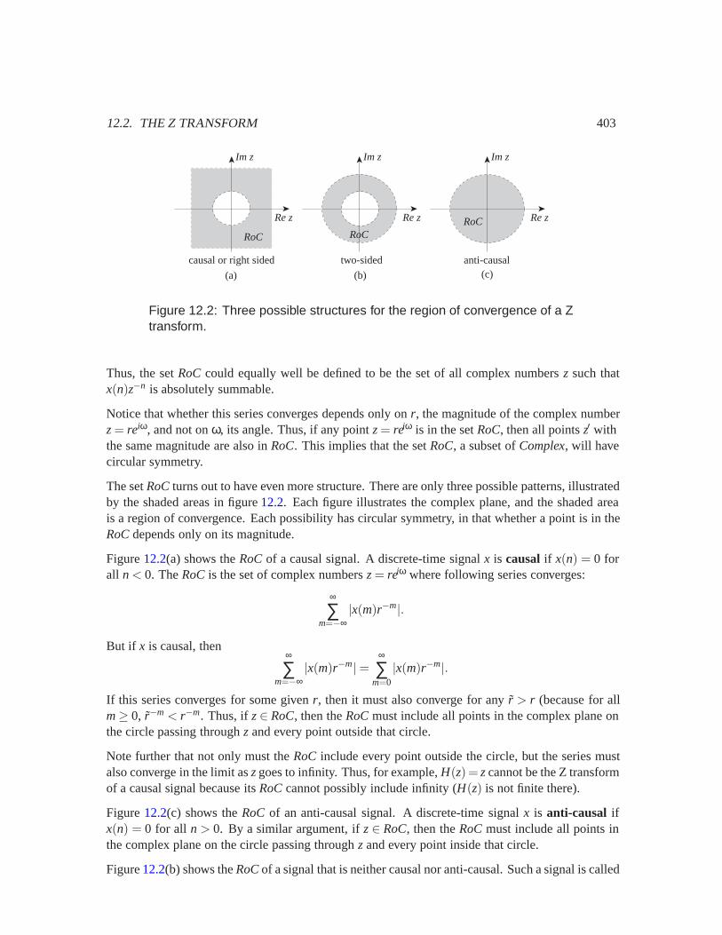
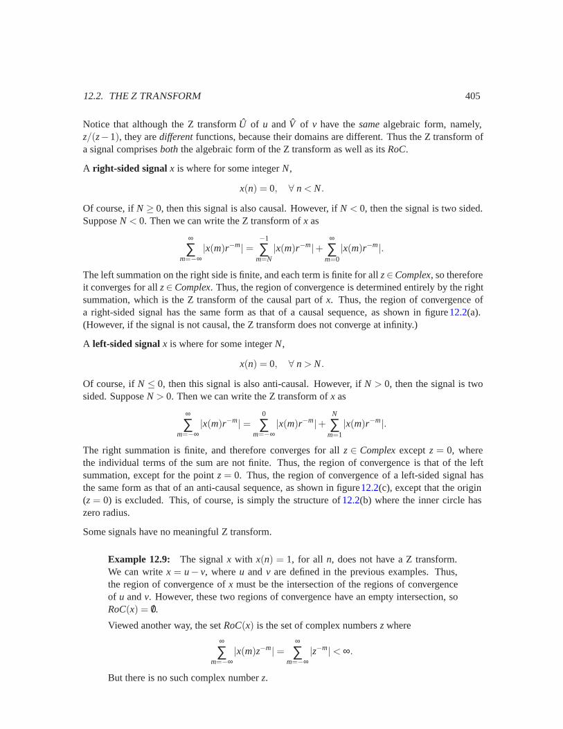
Figure 12.2: Three possible structures for the region of convergence of a Ztransform.
Thus, the set RoCcould equally well be defined to be the set of all complex numbers z such thatx(n)z−n is absolutely summable.
Notice that whether this series converges depends only on r , the magnitude of the complex numberz= reiω, and not on ω, its angle. Thus, if any point z= reiω is in the set RoC, then all points z′ withthe same magnitude are also in RoC. This implies that the set RoC, a subset of Complex, will havecircular symmetry.
The set RoCturns out to have even more structure. There are only three possible patterns, illustratedby the shaded areas in figure 12.2. Each figure illustrates the complex plane, and the shaded areais a region of convergence. Each possibility has circular symmetry, in that whether a point is in theRoCdepends only on its magnitude.
Figure 12.2(a) shows the RoCof a causal signal. A discrete-time signal x is causal if x(n) = 0 forall n < 0. The RoCis the set of complex numbers z= reiω where following series converges:
∞
∑m=−∞
|x(m)r−m|.
But if x is causal, then∞
∑m=−∞
|x(m)r−m|=∞
∑m=0
|x(m)r−m|.
If this series converges for some given r , then it must also converge for any r > r (because for allm≥ 0, r−m < r−m. Thus, if z∈ RoC, then the RoCmust include all points in the complex plane onthe circle passing through z and every point outside that circle.
Note further that not only must the RoC include every point outside the circle, but the series mustalso converge in the limit as zgoes to infinity. Thus, for example, H(z) = zcannot be the Z transformof a causal signal because its RoCcannot possibly include infinity (H(z) is not finite there).
Figure 12.2(c) shows the RoCof an anti-causal signal. A discrete-time signal x is anti-causal ifx(n) = 0 for all n > 0. By a similar argument, if z∈ RoC, then the RoCmust include all points inthe complex plane on the circle passing through z and every point inside that circle.
Figure 12.2(b) shows the RoCof a signal that is neither causal nor anti-causal. Such a signal is called
404 CHAPTER 12. STABILITY
a two-sided signal. Such a signal can always be expressed as a sum of a causal signal and an anti-causal signal. The RoCis the intersection of the regions of convergence for these two components.To see this, just note that the RoC is the set of complex numbers z = reiω where following seriesconverges:
∞
∑m=−∞
|x(m)r−m|=−1
∑m=−∞
|x(m)r−m|+∞
∑m=0
|x(m)r−m|.
The first sum on the right corresponds to an anti-causal signal, and the second sum on the right to acausal signal. For this series to converge, both sums must converge. Thus, for a two-sided signal,the RoChas a ring structure.
Example 12.7: Consider the discrete-time unit step signal u, given by
u(n) ={
0, n < 01, n≥ 0
. (12.13)
The Z transform is, using geometric series identity (12.9),
U(z) =∞
∑m=−∞
u(m)z−m =∞
∑m=0
z−m =1
1−z−1 =z
z−1,
with domain
RoC(u) = {z∈ Complex|∞
∑m=1
|z|−m < ∞}= {z | |z|> 1}.
This region of convergence has the structure of figure12.2(a), where the dashed circlehas radius one (that circle is called the unit circle). Indeed, this signal is causal, so thisstructure makes sense.
Example 12.8: The signal v given by
v(n) ={ −1, n < 0
0, n≥ 0,
has Z transform
V(z) =∞
∑m=−∞
v(m)z−m =−1
∑m=−∞
z−m =−z∞
∑k=0
zk =z
z−1,
with domain
RoC(v) = {z∈ Complex|1
∑m=−∞
|z|−m < ∞}= {z | |z|< 1}.
This region of convergence has the structure of figure12.2(c), where the dashed circleis again the unit circle. Indeed, this signal is anti-causal, so this structure makes sense.
12.2. THE Z TRANSFORM 405
Notice that although the Z transform U of u and V of v have the samealgebraic form, namely,z/(z−1), they are differentfunctions, because their domains are different. Thus the Z transform ofa signal comprises both the algebraic form of the Z transform as well as its RoC.
A right-sided signal x is where for some integer N,
x(n) = 0, ∀ n < N.
Of course, if N≥ 0, then this signal is also causal. However, if N < 0, then the signal is two sided.Suppose N < 0. Then we can write the Z transform of x as
∞
∑m=−∞
|x(m)r−m|=−1
∑m=N|x(m)r−m|+
∞
∑m=0
|x(m)r−m|.
The left summation on the right side is finite, and each term is finite for all z∈Complex, so thereforeit converges for all z∈Complex. Thus, the region of convergence is determined entirely by the rightsummation, which is the Z transform of the causal part of x. Thus, the region of convergence ofa right-sided signal has the same form as that of a causal sequence, as shown in figure 12.2(a).(However, if the signal is not causal, the Z transform does not converge at infinity.)
A left-sided signal x is where for some integer N,
x(n) = 0, ∀ n > N.
Of course, if N ≤ 0, then this signal is also anti-causal. However, if N > 0, then the signal is twosided. Suppose N > 0. Then we can write the Z transform of x as
∞
∑m=−∞
|x(m)r−m|=0
∑m=−∞
|x(m)r−m|+N
∑m=1
|x(m)r−m|.
The right summation is finite, and therefore converges for all z∈ Complexexcept z = 0, wherethe individual terms of the sum are not finite. Thus, the region of convergence is that of the leftsummation, except for the point z = 0. Thus, the region of convergence of a left-sided signal hasthe same form as that of an anti-causal sequence, as shown in figure12.2(c), except that the origin(z = 0) is excluded. This, of course, is simply the structure of 12.2(b) where the inner circle haszero radius.
Some signals have no meaningful Z transform.
Example 12.9: The signal x with x(n) = 1, for all n, does not have a Z transform.We can write x = u− v, where u and v are defined in the previous examples. Thus,the region of convergence of x must be the intersection of the regions of convergenceof u and v. However, these two regions of convergence have an empty intersection, soRoC(x) = /0.
Viewed another way, the set RoC(x) is the set of complex numbers z where
∞
∑m=−∞
|x(m)z−m|=∞
∑m=−∞
|z−m|< ∞.
But there is no such complex number z.
406 CHAPTER 12. STABILITY
Note that the signal x in example 12.9 is periodic with any integer period p (because x(n+ p) = x(n)for any p∈ Integers). Thus, it has a Fourier series representation. In fact, as shown in section10.6.3,a periodic signal also has a Fourier transform representation, as long as we are willing to allow Diracdelta functions in the Fourier transform. (Recall that this means that there are values of ω whereX(ω) will not be finite.) With periodic signals, the Fourier series is by far the simplest frequency-domain tool to use. The Fourier transform can also be used if we allow Dirac delta functions. TheZ transform, however, is more problematic, because the region of convergence is empty.
12.2.2 Stability and the Z transform
If a discrete-time signal x is absolutely summable, then it has a DTFT X that is finite for all ω∈Reals. Moreover, the DTFT is equal to the Z transform evaluated on the unit circle,
∀ ω∈ Reals, X(ω) = X(z)|z=eiω = X(eiω).
The complex number z= eiω has magnitude one, and therefore lies on the unit circle. Recall that anLTI system is stable if and only if its impulse response is absolutely summable. Thus,
A discrete-time LTI system with impulse response h is stable if and only if thetransfer function H, which is the Z transform of h, has a region of convergence thatincludes the unit circle.
Example 12.10: Continuing example 12.6, the transfer function of the bank accountsystem has region of convergence given by
RoC(h) = {z= reiω ∈ Complex| r > a},where a > 1. Thus, the region of convergence includes only complex numbers withmagnitude greater than one, and therefore does not include the unit circle. The bankaccount system is therefore not stable.
12.2.3 Rational Z tranforms and poles and zeros
All of the Z transforms we have seen so far are rational polynomials in z. A rational polynomial issimply the ratio of two finite-order polynomials. For example, the bank account system has transferfunction
H(z) =1
z−a
(see example 12.6). The unit step of example 12.7 and its anti-causal cousin of example 12.8 haveZ transforms given by
U(z) =z
z−1, V(z) =
zz−1
,
albeit with different regions of convergence.
12.2. THE Z TRANSFORM 407
In practice, most Z transforms of practical interest can be written as the ratio of two finite orderpolynomials in z,
X(z) =A(z)B(z)
.
The order of the polynomial A or B is the power of the highest power of z. For the unit step, thenumerator polynomial is A(z) = z, a first-order polynomial, and the denominator is B(z) = z− 1,also a first-order polynomial.
Recall from algebra that a polynomial of order N has N (possibly complex-valued) roots, whichare values of z where the polynomial evaluates to zero. The roots of the numerator A are called thezeroes of the Z transform, and the roots of the denominator B are called the poles of the Z transform.The term “zero” refers to the fact that the Z transform evaluates to zero at a zero. The term “pole”suggests an infinitely high tent pole, where the Z transform evaluates to infinity. The locations inthe complex plane of the poles and zeros turn out to yield considerable insight about a Z transform.A plot of these locations is called a pole-zero plot. The poles are shown as crosses and the zeros ascircles.
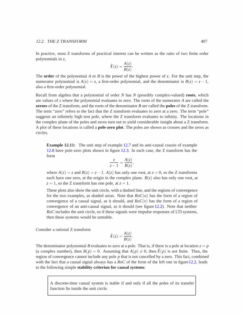
Example 12.11: The unit step of example 12.7 and its anti-causal cousin of example12.8 have pole-zero plots shown in figure 12.3. In each case, the Z transform has theform
zz−1
=A(z)B(z)
,
where A(z) = z and B(z) = z−1. A(z) has only one root, at z= 0, so the Z transformseach have one zero, at the origin in the complex plane. B(z) also has only one root, atz= 1, so the Z transform has one pole, at z= 1.
These plots also show the unit circle, with a dashed line, and the regions of convergencefor the two examples, as shaded areas. Note that RoC(u) has the form of a region ofconvergence of a causal signal, as it should, and RoC(v) has the form of a region ofconvergence of an anti-causal signal, as it should (see figure12.2). Note that neitherRoCincludes the unit circle, so if these signals were impulse responses of LTI systems,then these systems would be unstable.
Consider a rational Z transform
X(z) =A(z)B(z)
.
The denominator polynomial B evaluates to zero at a pole. That is, if there is a pole at location z= p(a complex number), then B(p) = 0. Assuming that A(p) �= 0, then X(p) is not finite. Thus, theregion of convergence cannot include any pole p that is not cancelled by a zero. This fact, combinedwith the fact that a causal signal always has a RoCof the form of the left one in figure12.2, leadsto the following simple stability criterion for causal systems:
A discrete-time causal system is stable if and only if all the poles of its transferfunction lie inside the unit circle.
408 CHAPTER 12. STABILITY
|z|=1
Re z
Im z
RoC(u) |z|=1
Re z
Im z
RoC(v)
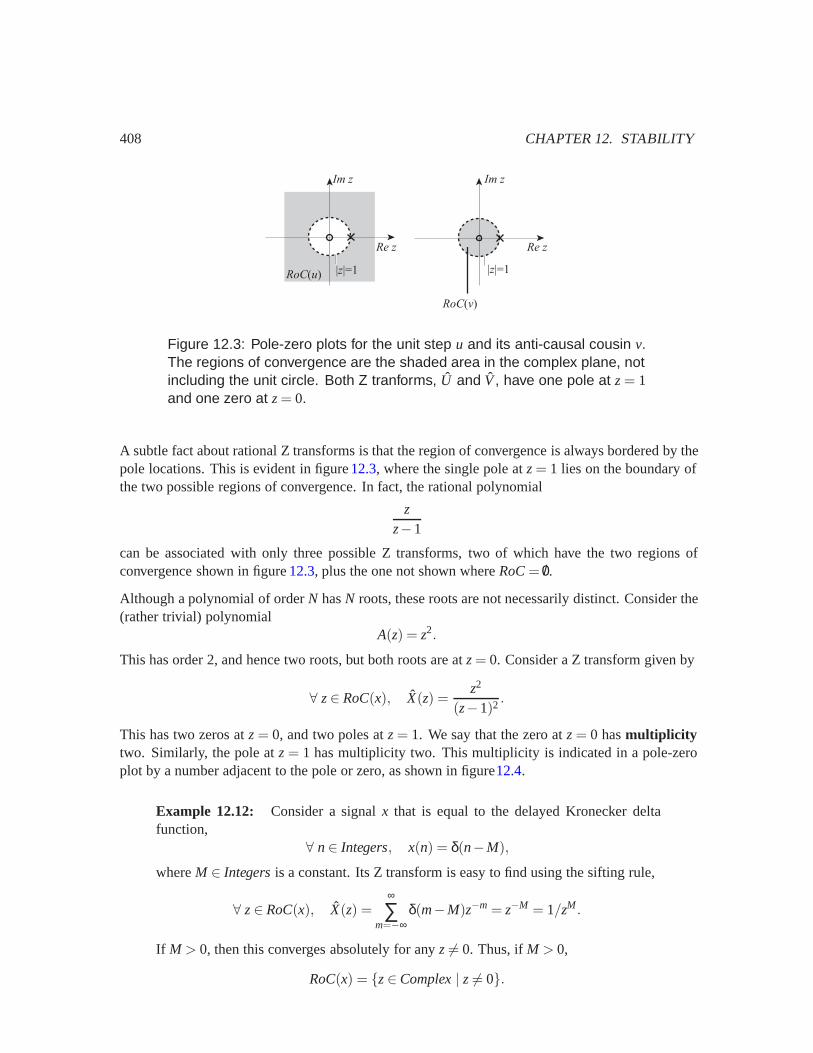
Figure 12.3: Pole-zero plots for the unit step u and its anti-causal cousin v.The regions of convergence are the shaded area in the complex plane, notincluding the unit circle. Both Z tranforms, U and V, have one pole at z= 1and one zero at z= 0.
A subtle fact about rational Z transforms is that the region of convergence is always bordered by thepole locations. This is evident in figure 12.3, where the single pole at z= 1 lies on the boundary ofthe two possible regions of convergence. In fact, the rational polynomial
zz−1
can be associated with only three possible Z transforms, two of which have the two regions ofconvergence shown in figure 12.3, plus the one not shown where RoC= /0.
Although a polynomial of order N has N roots, these roots are not necessarily distinct. Consider the(rather trivial) polynomial
A(z) = z2.
This has order 2, and hence two roots, but both roots are at z= 0. Consider a Z transform given by
∀ z∈ RoC(x), X(z) =z2
(z−1)2 .
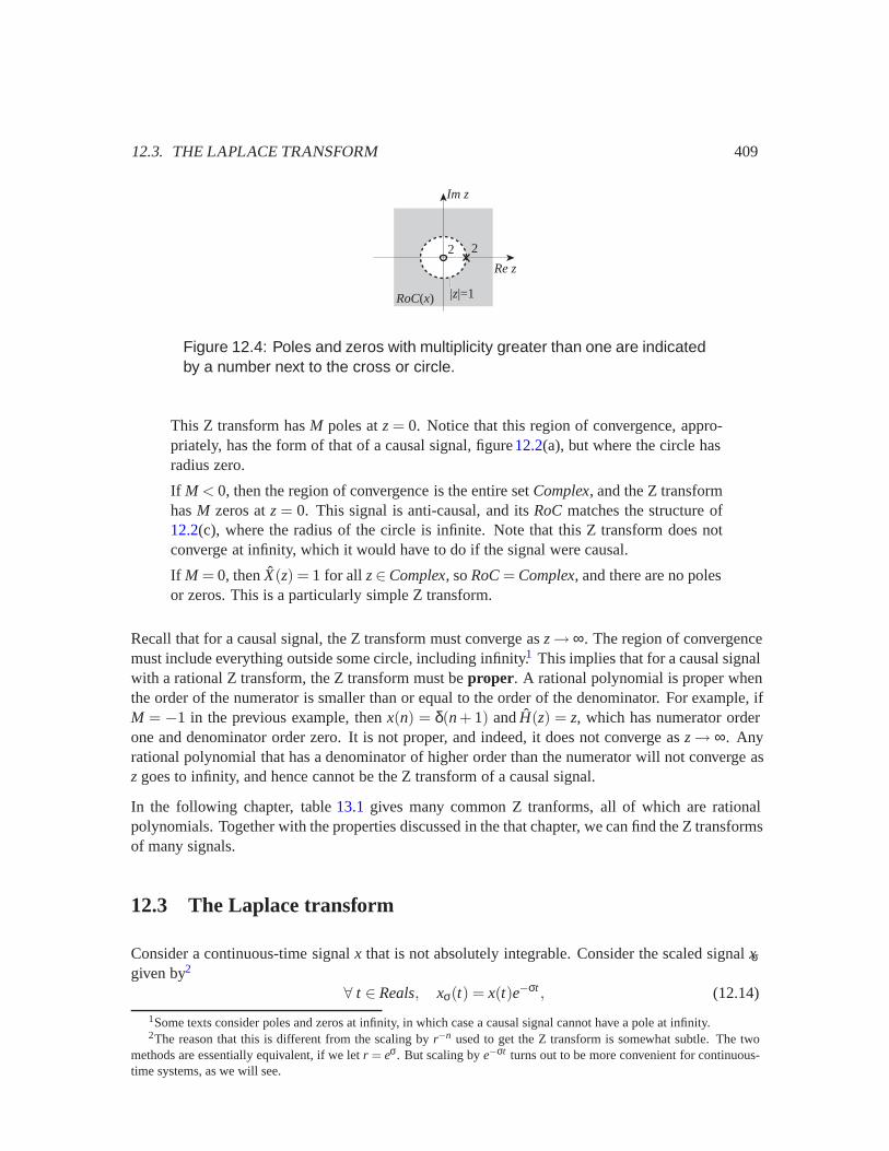
This has two zeros at z= 0, and two poles at z= 1. We say that the zero at z= 0 has multiplicitytwo. Similarly, the pole at z= 1 has multiplicity two. This multiplicity is indicated in a pole-zeroplot by a number adjacent to the pole or zero, as shown in figure12.4.
Example 12.12: Consider a signal x that is equal to the delayed Kronecker deltafunction,
∀ n∈ Integers, x(n) = δ(n−M),
where M ∈ Integersis a constant. Its Z transform is easy to find using the sifting rule,
∀ z∈RoC(x), X(z) =∞
∑m=−∞
δ(m−M)z−m = z−M = 1/zM .
If M > 0, then this converges absolutely for any z �= 0. Thus, if M > 0,
RoC(x) = {z∈Complex| z �= 0}.
12.3. THE LAPLACE TRANSFORM 409
|z|=1
Re z
Im z
RoC(x)
22
Figure 12.4: Poles and zeros with multiplicity greater than one are indicatedby a number next to the cross or circle.
This Z transform has M poles at z= 0. Notice that this region of convergence, appro-priately, has the form of that of a causal signal, figure12.2(a), but where the circle hasradius zero.
If M < 0, then the region of convergence is the entire set Complex, and the Z transformhas M zeros at z= 0. This signal is anti-causal, and its RoCmatches the structure of12.2(c), where the radius of the circle is infinite. Note that this Z transform does notconverge at infinity, which it would have to do if the signal were causal.
If M = 0, then X(z) = 1 for all z∈Complex, so RoC= Complex, and there are no polesor zeros. This is a particularly simple Z transform.
Recall that for a causal signal, the Z transform must converge as z→∞. The region of convergencemust include everything outside some circle, including infinity.1 This implies that for a causal signalwith a rational Z transform, the Z transform must be proper. A rational polynomial is proper whenthe order of the numerator is smaller than or equal to the order of the denominator. For example, ifM = −1 in the previous example, then x(n) = δ(n+ 1) and H(z) = z, which has numerator orderone and denominator order zero. It is not proper, and indeed, it does not converge as z→ ∞. Anyrational polynomial that has a denominator of higher order than the numerator will not converge asz goes to infinity, and hence cannot be the Z transform of a causal signal.
In the following chapter, table 13.1 gives many common Z tranforms, all of which are rationalpolynomials. Together with the properties discussed in the that chapter, we can find the Z transformsof many signals.
12.3 The Laplace transform
Consider a continuous-time signal x that is not absolutely integrable. Consider the scaled signal xσgiven by2
∀ t ∈Reals, xσ(t) = x(t)e−σt , (12.14)
1Some texts consider poles and zeros at infinity, in which case a causal signal cannot have a pole at infinity.2The reason that this is different from the scaling by r−n used to get the Z transform is somewhat subtle. The two
methods are essentially equivalent, if we let r = eσ. But scaling by e−σt turns out to be more convenient for continuous-time systems, as we will see.

410 CHAPTER 12. STABILITY
for some real number σ. Often, this signal is absolutely integrable when σ is chosen appropriately.This new signal, therefore, will have a CTFT, even if x does not.
Example 12.13: Consider the impulse response of the simplified helicopter systemdescribed in example 12.2. The output as a function of the input is given by
∀ t ∈ Reals, y(t) =1M
t∫0
x(τ)dτ.
The impulse response is found by letting the input be a Dirac delta function and usingthe sifting rule to get
∀ t ∈ Reals, h(t) = u(t)/M,
where u is the continuous-time unit step in (12.4). This is not absolutely integrable, sothis system is not stable. However, the scaled signal
∀ t ∈ Reals, hσ(t) = h(t)e−σt
is absolutely integrable if σ > 0. Its CTFT is
∀ σ > 0,∀ω∈ Reals, Hσ(ω) =∞∫−∞
h(t)e−σt e−iωtdt
=1M
∞∫0
e−σte−iωtdt
=1M
∞∫0
e−(σ+iω)tdt
=1
M(σ+ iω).
The last step in example 12.13 uses the following useful fact from calculus,
b∫a
ectdt =1c(ecb−eca) , (12.15)
for any c∈ Complexand a,b∈ Reals∪{−∞,∞} where ecb and eca are finite.
In general, the CTFT of the scaled signal xσ in (12.14) is
∀ ω∈ Reals, Xσ(ω) =∫ ∞
−∞x(t)e−(σ+iω)tdt.
Notice that this is a function not just of ω, but also of σ. We are only sure it is valid for values of σthat yield an absolutely integrable signal hσ.

12.3. THE LAPLACE TRANSFORM 411
Define the complex numbers= σ+ iω.
Then we can write this CTFT as
∀ s∈ RoC(x), X(s) =∞∫−∞
x(t)e−stdt, (12.16)
where X is a function called the Laplace transform of x,
X:RoC(x)→ Complex
where RoC(x) ⊂ Complexis given by
RoC(x) = {s= σ+ iω∈Complex| x(t)e−σt is absolutely integrable.} (12.17)
The Laplace tranform H of the impulse response h of an LTI system is called the transfer functionof the system, just as with discrete-time systems.
Example 12.14: Continuing example 12.13, we can recognize from the form of Hσ(ω)that the transfer function of the helicopter system is
∀ s∈RoC(h), H(s) =1
Ms.
The RoCisRoC(h) = {s= σ+ iω∈Complex| σ < 0}
12.3.1 Structure of the region of convergence
As with the Z transform, the region of convergence is an essential part of a Laplace transform. Itgives the domain of the function X. Whether a complex number s is in the RoCdepends only on σ,not on ω, as is evident in the definition (12.17). Since s= σ+ iω, whether a complex number is inthe region of convergence depends only on its real part. Once again, there are only three possiblepatterns for the region of convergence, shown in figure 12.5. Each figure illustrates the complexplane, and the shaded area is a region of convergence. Each possibility has vertical symmetry, inthat whether a point is in the RoCdepends only on its real part.
Figure 12.5(a) shows the RoCof a causal or right-sided signal. A continuous-time signal x is right-sided if x(t) = 0 for all t < T for some T ∈Reals. The RoCis the set of complex numbers s= σ+ iωwhere following integral converges:
∞∫−∞
|x(t)e−σt |dt.
But if x is right-sided, then∞∫−∞
|x(t)e−σt |dt =∞∫
T
|x(t)e−σt |dt.

412 CHAPTER 12. STABILITY
Re s
Im sIm s
Re s
Im s
causal or right-sided
Re s
anti-causal or left-sidedtwo-sided
RoC RoC RoC
(a) (b) (c)
Figure 12.5: Three possible structures for the region of convergence of aLaplace transform.
If T ≥ 0 and this integral converges for some given σ, then it must also converge for anyσ > σbecause for all t ≥ 0, e−σt < e−σt . Thus, if s= σ+ iω∈ RoC(x), then the RoC(x) must include allpoints in the complex plane on the vertical line passing through sand every point to the right of thatline.3
If T < 0, then∞∫
T
|x(t)e−σt |dt =0∫
T
|x(t)e−σt |dt +∞∫
0
|x(t)e−σt |dt,
then the finite integral exists and is finite for all σ, so the same argument applies.
Figure 12.5(c) shows the RoC of a left-sided signal. A continuous-time signal x is left-sided ifx(t) = 0 for all t > T for some T ∈ Reals. By a similar argument, if s= σ+ iω∈ RoC(x), then theRoC(x) must include all points in the complex plane on the vertical line passing through sand everypoint to the left of that line.
Figure 12.5(b) shows the RoCof a signal that is a two-sided signal. Such a signal can always beexpressed as a sum of a right-sided signal and left-sided signal. The RoCis the intersection of theregions of convergence for these two components.
Example 12.15: Using the same methods as in examples 12.13 and 12.14 we can findthe Laplace transform of the continuous-time unit step signal u, given by
∀ t ∈ Reals, u(t) ={
0, t < 01, t ≥ 0
. (12.18)
The Laplace transform is
∀ s∈RoC(u), U(s) =∞∫−∞
u(t)e−stdt
3It is convenient but coincidental that the region of convergence is the right half of a plane when the sequence is rightsided.
12.3. THE LAPLACE TRANSFORM 413
=∞∫
0
e−stdt
=1s,
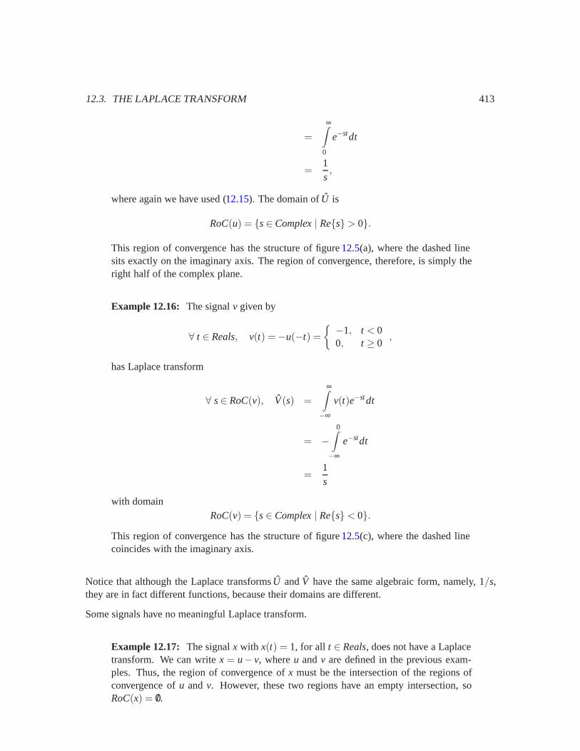
where again we have used (12.15). The domain of U is
RoC(u) = {s∈Complex| Re{s}> 0}.
This region of convergence has the structure of figure 12.5(a), where the dashed linesits exactly on the imaginary axis. The region of convergence, therefore, is simply theright half of the complex plane.
Example 12.16: The signal v given by
∀ t ∈ Reals, v(t) =−u(−t) ={ −1, t < 0
0, t ≥ 0,
has Laplace transform
∀ s∈ RoC(v), V(s) =∞∫−∞
v(t)e−stdt
= −0∫
−∞
e−stdt
=1s
with domainRoC(v) = {s∈ Complex| Re{s} < 0}.
This region of convergence has the structure of figure 12.5(c), where the dashed linecoincides with the imaginary axis.
Notice that although the Laplace transforms U and V have the same algebraic form, namely, 1/s,they are in fact different functions, because their domains are different.
Some signals have no meaningful Laplace transform.
Example 12.17: The signal x with x(t) = 1, for all t ∈ Reals, does not have a Laplacetransform. We can write x = u− v, where u and v are defined in the previous exam-ples. Thus, the region of convergence of x must be the intersection of the regions ofconvergence of u and v. However, these two regions have an empty intersection, soRoC(x) = /0.
414 CHAPTER 12. STABILITY
Viewed another way, the set RoC(x) is the set of complex numbers s where
∞∫−∞
|x(t)e−st|dt =∞∫−∞
|e−st|dt < ∞.
But there is no such complex number s.
Note that the signal x in example12.17 is periodic with any period p∈Reals(because x(t + p) = x(t)for any p∈ Reals). Thus, it has a Fourier series representation. In fact, as shown in section10.6.3,a periodic signal also has a Fourier transform representation, as long as we are willing to allowDirac delta functions in the Fourier transform. (Recall that this means that there are values ofω where X(ω) will not be finite.) In the continuous-time case as in the discrete-time case, withperiodic signals, the Fourier series is by far the simplest frequency-domain tool to use. The Fouriertransform can also be used if we allow Dirac delta functions. The Laplace transform, however, ismore problematic, because the region of convergence is empty.
12.3.2 Stability and the Laplace transform
If a continuous-time signal x is absolutely integrable, then it has a CTFT X that is finite for allω∈Reals. Moreover, the CTFT is equal to the Laplace transform evaluated on the imaginary axis,
∀ ω∈Reals, X(ω) = X(s)|s=iω = X(iω).
The complex number s= iω is pure imaginary, and therefore lies on the imaginary axis. Recall thatan LTI system is stable if and only if its impulse response is absolutely integrable. Thus
A continuous-time LTI system with impulse response h is stable if an only if thetransfer function H, which is the Laplace transform of h, has a region of conver-gence that includes the imaginary axis.
Example 12.18: Consider the exponential signal h given by
∀ t ∈ Reals, h(t) = e−atu(t),
for some real or complex number a, where, as usual, u is the unit step. The Laplacetransform is
∀ s∈ RoC(h), H(s) =∞∫−∞
h(t)e−stdt
=∞∫
0
e−ate−stdt

12.3. THE LAPLACE TRANSFORM 415
=∞∫
0
e−(s+a)tdt
=1
s+a,
where again we have used (12.15). It is evident from (12.15) that for this integral to bevalid, the domain of H must be
RoC(h) = {s∈ Complex| Re{s}>−Re{a}}.This region of convergence has the structure of figure12.5(a), where the vertical dashedline passes through a.
Now suppose that h is the impulse response of an LTI system. That LTI system is stableif an only if Re{a}> 0. Indeed, if Re{a}< 0, then the impulse response grows withoutbound, because e−at grows without bound as t gets large.
12.3.3 Rational Laplace tranforms and poles and zeros
All of the Laplace transforms we have seen so far are rational polynomials in s. In practice, mostLaplace transforms of interest can be written as the ratio of two finite order polynomials in s,
X(s) =A(s)B(s)
.
An exception is illustrated in the following example.
Example 12.19: Consider a signal x that is equal to the delayed Dirac delta function,
∀ t ∈ Reals, x(t) = δ(t− τ),
where τ ∈ Realsis a constant. Its Laplace transform is easy to find using the siftingrule,
∀ s∈ RoC(x), X(s) =∞∫−∞
δ(t− τ)e−stdt = e−sτ.
This has no finite-order rational polynomial representation.
Unlike the discrete-time case, pure time delays turn out to be rather difficult to realize in manyphysical systems that are studied using Laplace transforms, so we need not be overly concernedwith them. We focus henceforth on rational Laplace transforms.
For a rational Laplace transform, the order of the polynomial A or B is the power of the highestpower of s. For the exponential of example 12.18, the numerator polynomial is A(s) = 1, a zero-order polynomial, and the denominator is B(s) = s+ a, a first-order polynomial. As with the Ztransform, the roots of the numerator polynomial are called the zeros of the Laplace transform, andthe roots of the denominator polynomial are called the poles.

416 CHAPTER 12. STABILITY
Im s
Re s
RoC
s = − a
Figure 12.6: Pole-zero plot for the exponential signal of example 12.18,assuming a has a positive real part.
Example 12.20: The exponential of example 12.18 has a single pole at s=−a, and nozeros.4 A pole-zero plot is shown in figure 12.6, where we assume that a is a complexnumber with a positive real part. The region of convergence includes the imaginaryaxis, so this signal is absolutely integrable.
As with Z transforms, the region of convergence of a rational Laplace transform bordered by thepole locations. Hence,
A continuous-time causal system is stable if and only if all the poles of its transferfunction lie in the left half of the complex plane. That is, all the poles must havenegative real parts.
Table 13.3 in the following chapter gives many common Laplace tranforms.
12.4 Summary
Many useful signals have no Fourier transform. A sufficient condition for a signal to have a Fouriertransform that is finite at all frequencies is that the signal be absolutely summable (if it is a discrete-time signal) or absolutely integrable (if it is a continuous-time system).
Many useful systems are not stable, which means that even with a bounded input, the output maybe unbounded. An LTI system is stable if and only if its impulse response is absolutely summable(discrete-time) or absolutely integrable (continuous-time).
Many signals that are not absolutely summable (integrable) can be scaled by an exponential to geta new signal that is absolutely summable (integrable). The DTFT (CTFT) of the scaled signal iscalled the Z transform (Laplace transform) of the signal.
4In some texts, it will be observed that as s approaches infinity, this Laplace transform approaches zero, and hence itwill be said that there is a zero at infinity. So to avoid conflict with such texts, we might say that this Laplace transformhas no finite zeros.

12.4. SUMMARY 417
The Z transform (Laplace transform) is defined over a region of convergence, where the structureof the region of convergence depends on whether the signal is causal, anti-causal, or two-sided.The Z transform (Laplace transform) of the impulse response is called the transfer function of anLTI system. The region of convergence includes the unit circle (imaginary axis), if and only if thesystem is stable.
A rational Z transform (Laplace transform) has poles and zeros, and the poles bound the region ofconvergence. The locations of the poles and zeros yield considerable information about the system,including whether it is stable.
Exercises
Each problem is annotated with the letter E, T, C which stands for exercise, requires some thought,requires some conceptualization. Problems labeled E are usually mechanical, those labeled T re-quire a plan of attack, those labeled C usually have more than one defensible answer.
1. E Consider the signal x given by
∀ n∈ Integers, x(n) = anu(−n),
where a is a complex constant.
(a) Find the Z transform of x. Be sure to give the region of convergence.
(b) Where are the poles and zeros?
(c) Under what conditions on a is x absolutely summable?
(d) Assuming that x is absolutely summable, find its DTFT.
2. T Consider the signal x given by
∀ n∈ Integers, x(n) ={
1, |n| ≤M0, otherwise
,
for some integer M > 0.
(a) Find the Z transform of x. Simplify so that there remain no summations. Be sure to givethe region of convergence.
(b) Where are the poles and zeros? Do not give poles and zeros that cancel each other out.
(c) Under what conditions is x absolutely summable?
(d) Assuming that x is absolutely summable, find its DTFT.
3. T Consider the unit ramp signal w given by
∀ n∈ Integers, w(n) = nu(n),

418 CHAPTER 12. STABILITY
where u is the unit step. The following identity will be useful,
∞
∑m=0
(m+ 1)am = (∞
∑m=0
am)2 =1
(1−a)2 . (12.19)
This is a generalization of the geometric series identity, given by (12.9). This series convergesfor any complex number a with |a|< 1, because
∞
∑m=0
(m+ 1)|a|m = 1+ 2|a|+ 3|a|2 + · · ·
= (1+ |a|+ |a|2 + · · ·)(1+ |a|+ |a|2 + · · ·)= (
∞
∑m=0
|a|m)2
< ∞.
(a) Use the given identity to find the Z transform of the unit ramp. Be sure to give the regionof convergence. Check your answer against that given on page432.
(b) Sketch the pole-zero plot of the Z transform.
(c) Is the unit ramp absolutely summable?
4. E Sketch the pole-zero plots and regions of convergence for the Z transforms of the follow-ing impulse responses, and indicate whether a discrete-time LTI system with these impulseresponses is stable:
(a) h1(n) = δ(n)+ 0.5δ(n−1).
(b) h2(n) = (0.5)nu(n).
(c) h3(n) = 2nu(n).
5. E Consider the anti-causal continuous-time exponential signal x given by
∀ t ∈Reals, x(t) =−e−atu(−t),
for some real or complex number a, where, as usual, u is the unit step.
(a) Show that the Laplace transform of x is
X(s) =1
s+a
with region of convergence
RoC(x) = {s∈ Complex| Re{s} <−Re{a}}.
(b) Where are the poles and zeros?
(c) Under what conditions on a is x absolutely integrable?
(d) Assuming that x is absolutely integrable, find its CTFT.

12.4. SUMMARY 419
6. E This exercise demonstrates that the Laplace transform is linear. Show that if x and y arecontinuous-time signals, a and b are complex (or real) constants, and w is given by
∀ t ∈Reals, w(t) = ax(t)+by(t),
then the Laplace transform is
∀ s∈ RoC(w), W(s) = aX(s)+bY(s),
whereRoC(w)⊃RoC(x)∩RoC(y).
7. T Let the causal sinusoidal signal y be given by
∀ t ∈ Reals, y(t) = cos(ω0t)u(t),
where ω0 is a real number and u is the unit step.
(a) Show that the Laplace transform is
∀ s∈ {s | Re{s}> 0}, Y(s) =s
s2 +ω20
.
Hint: Use linearity, demonstrated in exercise 6, and Euler’s relation.
(b) Sketch the pole-zero plot and show the region of convergence.
8. E Consider a discrete-time LTI system with impulse response
∀n, h(n) = an cos(ω0n)u(n),
for some ω0 ∈Reals. Determine for what values of a this system is stable.
9. T The continuous-time unit ramp signal w is given by
∀t ∈Reals, x(t) = tu(t),
where u is the unit step.
(a) Find the Laplace transform of the unit ramp, and give the region of convergence.Hint: Use integration by parts in (12.16) and the fact that
∫ ∞0 te−σtdt < ∞ for σ > 0.
(b) Sketch the pole-zero plot of the Laplace transform.
10. E Let h and g be the impulse response of two stable systems. They may be discrete-time orcontinuous-time. Let a and b be two complex numbers. Show that the system with impulseresponse ah+bg is stable.
11. T Consider a series composition of two (continuous- or discrete-time) systems with impulseresponse h and g. The output v of the first system is related to its input x by v = h∗x. Theoutput y of the second system (and of the series composition) is y = g∗ v. Suppose bothsystems are stable. Show that the series composition is stable.Hint: Use the definition of stability.
420 CHAPTER 12. STABILITY
x y
h1
h2 g2
g1
+
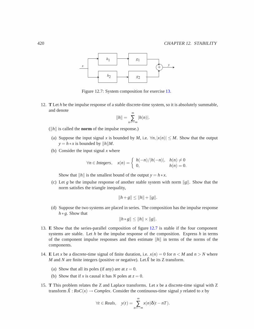
Figure 12.7: System composition for exercise 13.
12. T Let h be the impulse response of a stable discrete-time system, so it is absolutely summable,and denote
‖h‖=∞
∑n=−∞
|h(n)|.
(‖h‖ is called the norm of the impulse response.)
(a) Suppose the input signal x is bounded by M, i.e. ∀n, |x(n)| ≤M. Show that the outputy = h∗x is bounded by ‖h‖M.
(b) Consider the input signal x where
∀n∈ Integers, x(n) ={
h(−n)/|h(−n)|, h(n) �= 00, h(n) = 0.
Show that ‖h‖ is the smallest bound of the output y = h∗x.
(c) Let g be the impulse response of another stable system with norm ‖g‖. Show that thenorm satisfies the triangle inequality,
‖h+g‖ ≤ ‖h‖+‖g‖.
(d) Suppose the two systems are placed in series. The composition has the impulse responseh∗g. Show that
‖h∗g‖ ≤ ‖h‖×‖g‖.13. E Show that the series-parallel composition of figure 12.7 is stable if the four component
systems are stable. Let h be the impulse response of the composition. Express h in termsof the component impulse responses and then estimate ‖h‖ in terms of the norms of thecomponents.
14. E Let x be a discrete-time signal of finite duration, i.e. x(n) = 0 for n < M and n > N whereM and N are finite integers (positive or negative). Let X be its Z transform.
(a) Show that all its poles (if any) are at z= 0.
(b) Show that if x is causal it has N poles at z= 0.
15. T This problem relates the Z and Laplace transforms. Let x be a discrete-time signal with Ztransform X : RoC(x)→ Complex. Consider the continuous-time signal y related to x by
∀t ∈Reals, y(t) =∞
∑n=−∞
x(n)δ(t−nT).
12.4. SUMMARY 421
Here T > 0 is a fixed period. So y comprises delta functions located at t = nT of magnitudex(n).
(a) Use the sifting property and the definition (12.16) to find the Laplace transform Y of y.What is RoC(y)?
(b) Show that Y(s) = X(esT), where X(esT) is X(z) evaluated at s= esT.
(c) Suppose X(z) = 1z−1 with RoC(x) = {z | |z|> 1}. What are Y and RoC(y)?

422 CHAPTER 12. STABILITY
Chapter 13
Laplace and Z Transforms
In the previous chapter, we defined Laplace and Z transforms to deal with signals that are notabsolutely summable and systems that are not stable. The Z transform of the discrete-time signal xis given by
∀ z∈ RoC(x), X(z) =∞
∑m=−∞
x(m)z−m,
where RoC(x) is the region of convergence, the region in which the sum above converges abso-lutely.
The Laplace transform of the continuous-time signal x is given by
∀ s∈ RoC(x), X(s) =∞∫−∞
x(t)e−stdt,
where RoC(x) is again the region of convergence, the region in which the integral above convergesabsolutely.
In this chapter, we explore key properties of the Z and Laplace transforms and give examples oftransforms. We will also explain how, given a rational polynomial in z or s, plus a region of con-vergence, one can find the corresponding time-domain function. This inverse transform provesparticularly useful, because compositions of LTI systems, studied in the next chapter, often lead torather complicated rational polynomial descriptions of a transfer function.
Z transforms of common signals are given in table 13.1. Properties of the Z transform are summa-rized in table 13.2 and elaborated in the first section below.
13.1 Properties of the Z tranform
The Z transform has useful properties that are similar to those of the four Fourier transforms. Theyare summarized in table 13.2 and elaborated in this section.
423

424 CHAPTER 13. LAPLACE AND Z TRANSFORMS
Discrete-time signal∀ n∈ Integers
Z transform∀ z∈ RoC(x)
Roc(x)⊂ Complex Reference
x(n) = δ(n−M) X(z) = z−M Complex Example12.12
x(n) = u(n) X(z) = zz−1
{z | |z|> 1} Example12.7
x(n) = anu(n) X(z) = zz−a
{z | |z|> |a|} Example13.3
x(n) = anu(−n) X(z) = 11−a−1z
{z | |z|< |a|} Exercise 1in chapter
12
x(n) = cos(ω0n)u(n) X(z) = z2−zcos(ω0)z2−2zcos(ω0)+1
{z | |z|> 1} Example13.3
x(n) = sin(ω0n)u(n) X(z) = zsin(ω0)z2−2zcos(ω0)+1 , {z | |z|> 1} Exercise 1
x(n) =1
(N−1)! (n−1) · · · (n−N +1)
an−Nu(n−N)
X(z) = 1(z−a)N
{z | |z|> |a|} ( 13.13)
x(n) =(−1)N
(N−1)! (N−1−n) · · · (1−n)
an−Nu(−n)
X(z) = 1(z−a)N
{z | |z|< |a|} (13.14)
Table 13.1: Z transforms of key signals. The signal u is the unit step (12.13),δ is the Kronecker delta, a is any complex constant, ω0 is any real constant,M is any integer constant, and N > 0 is any integer constant.
13.1. PROPERTIES OF THE Z TRANFORM 425
Time domain∀ n∈ Integers
Frequency domain∀ z∈RoC
RoC Name(reference)
w(n) = ax(n)+by(n) W(z) = aX(z)+bY(z) RoC(w)⊃ RoC(x)∩RoC(y) Linearity(section 13.1.1)
y(n) = x(n−N) Y(z) = z−NX(z) RoC(y) = RoC(x) Delay(section 13.1.2)
y(n) = (x∗h)(n) Y(z) = X(z)H(z) RoC(y)⊃RoC(x)∩RoC(h) Convolution(section 13.1.3)
y(n) = x∗(n) Y(z) = [X(z∗)]∗ RoC(y) = RoC(x) Conjugation(section 13.1.4)
y(n) = x(−n) Y(z) = X(z−1) RoC(y) ={z | z−1 ∈RoC(x)}
Time reversal(section 13.1.5)
y(n) = nx(n) Y(z) =−z ddzX(z) RoC(y) = RoC(x) Scaling by n
(page 432)
y(n) = a−nx(n) Y(z) = X(az) RoC(y) ={z | az∈RoC(x)}
Exponentialscaling
(section 13.1.6)
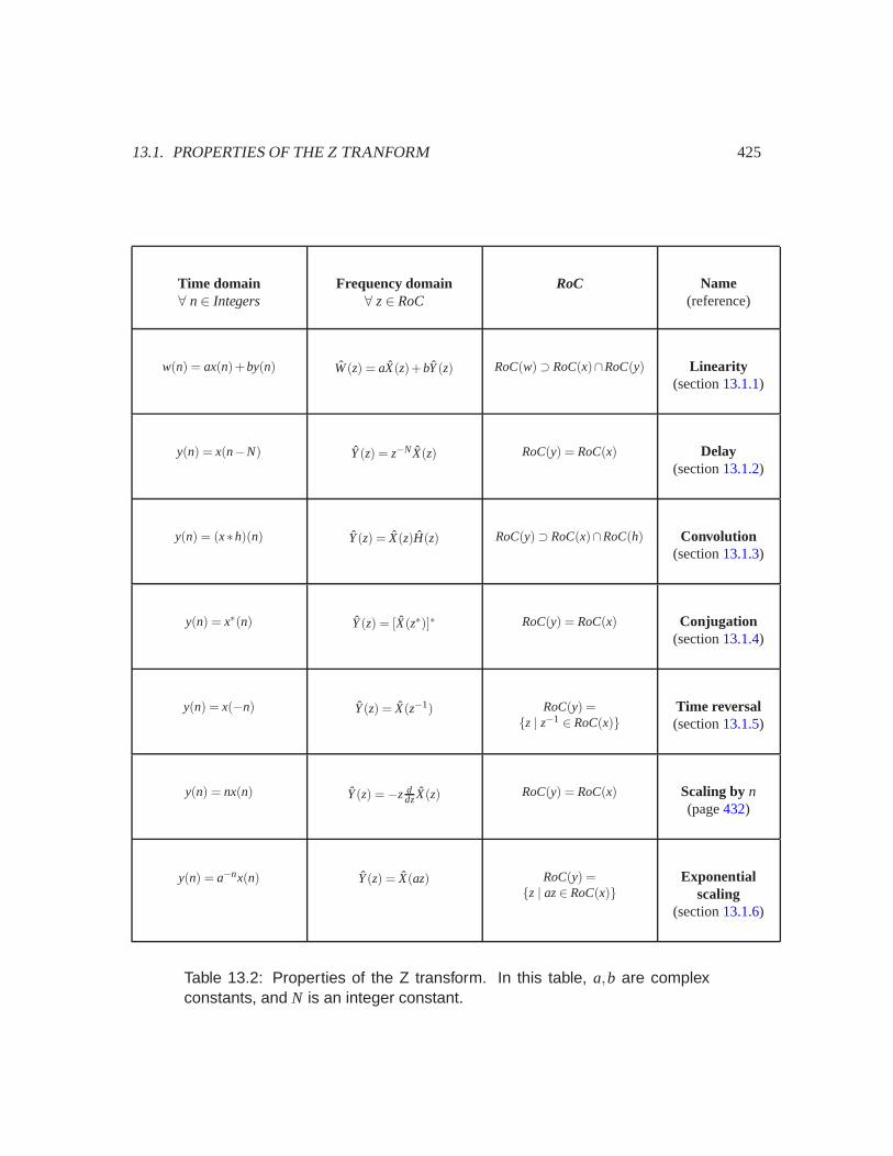
Table 13.2: Properties of the Z transform. In this table, a,b are complexconstants, and N is an integer constant.

426 CHAPTER 13. LAPLACE AND Z TRANSFORMS
13.1.1 Linearity
Suppose x and y have Z transforms X and Y, that a,b are two complex constants, and that
w = ax+by.
Then the Z transform of w is
∀ z∈ RoC(w), W(z) = aX(z)+bY(z).
This follows immediately from the definition of the Z transform,
W(z) =∞
∑m=−∞
w(m)z−m
=∞
∑m=−∞
(ax(m)+by(m))z−m
= aX(z)+bY(z).
The region of convergence of w must include at least the regions of convergence of x and y, sinceif x(n)r−n and y(n)r−n are absolutely summable, then certainly (ax(n) + by(n))r−n is absolutelysummable. Conceivably, however, the region of convergence may be larger. Thus, all we can assertin general is
RoC(w)⊃ RoC(x)∩RoC(y). (13.1)
Linearity is extremely useful because it makes it easy to find the Z transform of complicated signalsthat can be expressed a linear combination of signals with known Z transforms.
Example 13.1: We can use the results of example 12.12 plus linearity to find, forexample, the Z transform of the signal x given by
∀ n∈ Integers, x(n) = δ(n)+ 0.9δ(n−4)+ 0.8δ(n−5).
This is simply
X(z) = 1+ 0.9z−4 + 0.8z−5.
We can identify the poles by writing this as a rational polynomial in z (multiply top andbottom by z5),
X(z) =z5 + 0.9z+ 0.8
z5 ,
from which we see that there are 5 poles at z= 0. The signal is causal, so the regionof convergence is the region outside the circle passing through the pole with the largestmagnitude, or in this case,
RoC(x) = {z∈Complex| z �= 0}.
13.1. PROPERTIES OF THE Z TRANFORM 427
Example 13.1 illustrates how to find the transfer function of any finite impulse response (FIR) filter.It also suggests that the transfer function of an FIR filter always has a region of convergence thatincludes the entire complex plane, except possibly z= 0. The region of convergence will also notinclude z= ∞ if the FIR filter is not causal.
Linearity can also be used to invert a Z transform. That is, given a rational polynomial and a regionof convergence, we can find the time-domain function that has this Z transform. The general methodfor doing this will be considered in the next chapter, but for certain simple cases, we just have torecognize familiar Z transforms.
Example 13.2: Suppose we are given the Z transform
∀ z∈ {z∈ Complex| z �= 0}, X(z) =z5 + 0.9z+ 0.8
z5 .
We can immediately recognize this as the Z transform of a causal signal, because it is aproper rational polynomial and the region of convergence includes the entire complexplane except z= 0 (thus, it has the form of figure 12.2(a)).
If we divide through by z5, this becomes
∀ z∈ {z∈ Complex| z �= 0}, X(z) = 1+ 0.9z−4 + 0.8z−5.
By linearity, we can see that
∀ n∈ Integers, x(n) = x1(n)+ 0.9x2(n)+ 0.8x3(n),
where x1 has Z transform 1, x2 has Z transform z−4, and x3 has Z transform z−5. Theregions of convergence for each Z transform must be at least that of x, or at least {z∈Complex| z �= 0}. From example 12.12, we recognize these Z transforms, and henceobtain
∀ n∈ Integers, x(n) = δ(n)+ 0.9δ(n−4)+ 0.8δ(n−5).
Another application of linearity uses Euler’s relation to deal with sinusiodal signals.
Example 13.3: Consider the exponential signal x given by
∀ n∈ Integers, x(n) = anu(n),
where a is a complex constant. Its Z transform is
X(z) =∞
∑m=−∞
x(m)z−m =∞
∑m=0
amz−m =1
1−az−1 =z
z−a, (13.2)
where we have used the geometric series identity (12.9). This has a zero at z= 0 and apole at z= a. The region of convergence is
RoC(x) = {z∈ Complex|∞
∑m=0
|a|m|z|−m < ∞}= {z | |z|> |a|}, (13.3)
428 CHAPTER 13. LAPLACE AND Z TRANSFORMS
Re z
Im z
RoC(x) |z|=1
Re z
Im z
RoC(y)
a
|z|=|a|
eiω0
e-iω0
(a) (b)
Figure 13.1: Pole-zero plots for the exponential signal x and the sinusoidalsignal y of example 13.3.
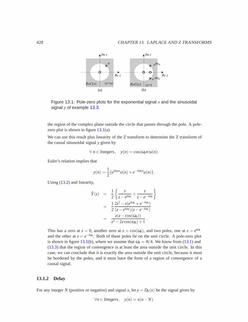
the region of the complex plane outside the circle that passes through the pole. A pole-zero plot is shown in figure 13.1(a).
We can use this result plus linearity of the Z transform to determine the Z transform ofthe causal sinusoidal signal y given by
∀ n∈ Integers, y(n) = cos(ω0n)u(n).
Euler’s relation implies that
y(n) =12{eiω0nu(n)+e−iω0nu(n)}.
Using (13.2) and linearity,
Y(z) =12
{z
z−eiω0+
zz−e−iω0
}
=12
2z2−z(eiω0 +e−iω0)(z−eiω0)(z−e−iω0)
=z(z− cos(ω0))
z2−2zcos(ω0)+ 1.
This has a zero at z = 0, another zero at z = cos(ω0), and two poles, one at z = eiω0
and the other at z= e−iω0 . Both of these poles lie on the unit circle. A pole-zero plotis shown in figure 13.1(b), where we assume that ω0 = π/4. We know from (13.1) and(13.3) that the region of convergence is at least the area outside the unit circle. In thiscase, we can conclude that it is exactly the area outside the unit circle, because it mustbe bordered by the poles, and it must have the form of a region of convergence of acausal signal.
13.1.2 Delay
For any integer N (positive or negative) and signal x, let y = DN(x) be the signal given by
∀n∈ Integers, y(n) = x(n−N).
13.1. PROPERTIES OF THE Z TRANFORM 429
Suppose x has Z transform X with domain RoC(x). Then RoC(y) = RoC(x) and
∀z∈ RoC(y), Y(z) =∞
∑m=−∞
y(m)z−m =∞
∑m=−∞
x(m−N)z−m = z−NX(z). (13.4)
Thus
If a signal is delayed by N samples, its Z transform is multiplied by z−N.
13.1.3 Convolution
Suppose x and h have Z transforms X and H. Let
y = x∗h.
Then∀z∈ RoC(y), Y(z) = X(z)H(z). (13.5)
This follows from using the definition of convolution,
∀n∈ Integers, y(n) =∞
∑m=−∞
x(m)h(n−m),
in the definition of the Z transform,
Y(z) =∞
∑n=−∞
y(n)z−n =∞
∑n=−∞
∞
∑m=−∞
x(m)z−mh(n−m)z−(n−m)
=∞
∑l=−∞
∞
∑m=−∞
x(m)z−mh(l)z−l = X(z)H(z).
The Z transform of y converges absolutely at least at values of z where both X and H convergeabsolutely. Thus,
RoC(y)⊃ RoC(x)∩RoC(h).
This is true because the double sum above can be written as
∞
∑n=−∞
y(n)z−n =
(∞
∑m=−∞
x(m)z−m
)(∞
∑l=−∞
h(l)z−l
).
This obviously converges absolutely if each of the two factors converges absolutely. Note that theregion of convergence may actually be larger than RoC(x)∩RoC(h). This can occur, for example,if the product (13.5) results in zeros of X(z) cancelling poles of H(z) (see exercise 3).
If h is the impulse response of an LTI system, then its Z transform is called the transfer functionof the system. The result (13.5) tells us that the Z transform of the output is the product of the Ztransform of the input and the transfer function. The transfer function, therefore, serves the samerole as the frequency response. It converts convolution into simple multiplication.
430 CHAPTER 13. LAPLACE AND Z TRANSFORMS
13.1.4 Conjugation
Suppose x is a complex-valued signal. Let y be defined by
∀ n∈ Integers, y(n) = [x(n)]∗.
Then∀ z∈ RoC(y), Y(z) = [X(z∗)]∗,
whereRoC(y) = RoC(x).
This follows because
∀ z∈ RoC(x), Y(z) =∞
∑n=−∞
y(n)z−n
=∞
∑n=−∞
x∗(n)z−n
=
[∞
∑n=−∞
x(n)(z∗)−n
]∗= [X(z∗)]∗.
If x happens to be a real signal, then y = x, soY = X, so
X(z) = [X(z∗)]∗.
The key consequence is:
For the Z transform of a real-valued signal, poles and zeros occur in complex-conjugate pairs. That is, if there is a zero at z = q, then there must be a zero atz= q∗, and if there is a pole at z= p, then there must be a pole at z= p∗.
This is because0 = X(q) = (X(q∗))∗
Similarly, if there is a pole at z= p, then there must also be a pole at z= p∗.
Example 13.4: Example 13.3 gave the Z transform of a signal of the form x(n) =anu(n), where a is allowed to be complex, and the Z tranform of a signal of the formy(n) = cos(ω0n)u(n), which is real-valued. The pole-zero plots are shown in figure13.1. In that figure, the complex signal has a pole at z = a, and none at z = a∗. Butthe real signal has a pole at z = eiω0 and a matching pole at the complex conjugate,z= e−iω0 .
13.1. PROPERTIES OF THE Z TRANFORM 431
13.1.5 Time reversal
Suppose x has Z transform X and y is obtained from x by reversing time, so that
∀ n∈ Integers, y(n) = x(−n).
Then∀z∈ {z∈ Complex| z−1 ∈ Roc(x)}, Y(z) = X(z−1).
This is evident from the definition of the Z transform, which implies that
Y(z) =∞
∑m=−∞
x(−m)z−m =∞
∑n=−∞
x(n)(z−1)−n = X(z−1),
where X(z−1) is X evaluated at z−1.
13.1.6 Multiplication by an exponential
Suppose x has Z transform X, a is a complex constant, and y(n) = a−nx(n) for all n. Then
∀z∈ {z∈Complex| az∈RoC(x)}, Y(z) = X(az),
where X(az) is X evaluated at az. This is because
Y(z) =∞
∑m=−∞
y(m)z−m =∞
∑m=−∞
x(m)(az)−m = X(az).
Note that if X has a pole at p (or a zero at q), then Y has a pole at p/a (or a zero at q/a).
Example 13.5: Suppose x is given by
∀ n∈ Integers, x(n) = anu(n).
Then we know from example 13.3 that
∀ z∈ {z | |z|> |a|}, X(z) =z
z−a.
This has a pole at z= a. Now let y(n) = a−nx(n) = u(n). The Z transform is
Y(z) = X(az) =az
az−a=
zz−1
,
as expected. Moreover, this has a pole at z= a/a = 1, as expected, and the region ofconvergence is indeed given by
{z∈ Complex| az∈ RoC(x)} = {z∈ Complex| |z|> 1}.
432 CHAPTER 13. LAPLACE AND Z TRANSFORMS
Probing further: Derivatives of Z transforms
Calculus on complex-valued functions of complex variables can be somewhat intri-cate. Suppose X is a function of a complex variable. The derivative can be definedas a limit,
ddz
X(z) = limε→0
X(z+ ε)− X(z)ε
,
where ε is a complex variable that can approach zero from any direction in thecomplex plane. The derivative exists if the limit does not depend on the direction.If the derivative exists at all points within a distance ε > 0 of a point z in the complexplane, then X is said to be analytic at z. A Z transform is a series of the form
∀ z∈ RoC(x), X(z) =∞
∑n=−∞
x(n)z−n.
This is called a Laurent series in the theory of complex variables. It can be shownthat a Laurent series is analytic at all points z∈ RoC(x), and that the derivative is
∀ z∈ RoC(x),ddz
X(z) =∞
∑m=−∞
−mx(m)z−m−1.
We can use this fact to show that the Z transform of y given by y(n) = nx(n) is
∀z∈Roc(x), Y(z) =−zddz
X(z).
This is because
Y(z) =∞
∑n=−∞
nx(n)z−n =∞
∑n=−∞
(−z)ddz
x(n)z−n =−zddz
X(z).
It is not difficult to show that Roc(y) = Roc(x) (see exercise 5).
This property can be used to find other Z transforms. For example, the Z transformof the unit step, x = u, is X(z) = z/(z−1), with RoC(x) = {z∈Complex| |z|> 1}.So the Z transform of the unit ramp y, given by y(n) = nu(n), is
Y(z) =−zddz
zz−1
=z
(z−1)2 ,
with RoC(y) = {z∈Complex| |z|> 1}. Another method for finding the Z transformof the unit ramp is given in exercise 3 of chapter 12.
13.1. PROPERTIES OF THE Z TRANFORM 433
13.1.7 Causal signals and the initial value theorem
Consider a causal discrete-time signal x. Its Z transform is
∀ z∈ {z∈ Complex| |z|> r}, X(z) =∞
∑m=0
x(m)z−m,
for some r (the largest magnitude of a pole). Then
limz→∞
∞
∑m=0
x(m)z−m = x(0)+ limz→∞
∞
∑m=1
x(m)z−m = x(0).
This is because as z goes to ∞, each term x(m)z−m goes to zero. Thus
If x is causal, x(0) = limz→∞
X(z) .
This is called the initial value theorem.
Example 13.6: The Z transform of the unit step x(n) = u(n) is X(z) = z/(z−1), so, asexpected,
x(0) = limz→∞
X(z) = limz→∞
zz−1
= limz→∞
11−z−1 = 1,
becauselimz→∞
z−1 = 0.
Suppose a Z transform X is the rational polynomial
X(z) =aMzM +aM−1zM−1 · · ·+a0
zN +bN−1zN−1 + · · ·+b0.
If x is causal, then this rational polynomial must be proper. Were this not the case, if M > N, thenby the initial value theorem, we would have
x(0) = limz→∞
X(z) = ∞,
which is certainly not right.
Example 13.7: Consider the Z transform
∀ z∈ Complex, X(z) = z.
This is not a proper rational polynomial (the numerator has order 1 and the denominator,which is 1, has order 0). From example 12.12, we know that this corresponds to
∀ n∈ Integers, x(n) = δ(n+ 1).
This is not a causal signal.
434 CHAPTER 13. LAPLACE AND Z TRANSFORMS
13.2 Frequency response and pole-zero plots
A pole-zero plot can be used to get a quick estimate of key properties of an LTI system. We havealready seen that it reveals whether the system is stable. It also reveals key features of the frequencyresponse, such as whether the system is highpass or lowpass.
Consider a stable discrete-time LTI system with impulse response h, frequency response H , andrational transfer function H. We know that the frequency response and transfer function are relatedby
∀ω∈ Reals, H(ω) = H(eiω).
That is, the frequency response is equal to the Z transform evaluated on the unit circle. The unitcircle is in the region of convergence because the system is stable.
Assume that H is a rational polynomial, in which case we can express it in terms of the first-orderfactors of the numerator and denominator polynomials,
H(z) =(z−q1) · · · (z−qM)(z− p1) · · · (z− pN)
,
with zeros at q1, · · · ,qM and poles at p1, · · · , pN. The zeros and poles may be repeated (i.e., they mayhave multiplicity greater than one). The frequency response is therefore
∀ ω∈ Reals, H(ω) =(eiω−q1) · · · (eiω−qM)(eiω− p1) · · · (eiω− pN)
.
The magnitude response is
∀ ω∈ Reals, |H(ω)|= |eiω−q1| · · · |eiω−qM||eiω− p1| · · · |eiω− pN| .
Each of these factors has the form|eiω−b|
where b is the location of either a pole or a zero. The factor |eiω−b| is just the distance from eiω tob in the complex plane.
Of course, eiω is a point on the unit circle. If that point is close to a zero at location q, then the factor|eiω−q| is small, so the magnitude response will be small. If that point is close to a pole at p, thenthe factor |eiω− p| is small, but since this factor is in the denominator, the magnitude response willbe large. Thus,
The magnitude response of a stable LTI system may be estimated from the pole-zero plot of its transfer function. Starting at ω= 0, trace counterclockwise aroundthe unit circle as ω increases. If you pass near a zero, then the magnitude responseshould dip. If you pass near a pole, then the magnitude response should rise.
13.2. FREQUENCY RESPONSE AND POLE-ZERO PLOTS 435
Example 13.8: Consider the causal LTI system of example 9.16, which is defined bythe difference equation
∀ n∈ Integers, y(n) = x(n)+ 0.9y(n−1).
We can find the transfer function by taking Z transforms on both sides, using linearity,to get
Y(z) = X(z)+ 0.9z−1Y(z).
The transfer function is
H(z) =Y(z)X(z)
=1
1−0.9z−1 =z
z−0.9.
This has a pole at z = 0.9, which is closest to z = 1 on the unit circle, and a zero atz= 0, which is equidistant from all points on the unit circle. The zero, therefore, hasno effect on the magnitude response. The pole is closest to z= 1, which corresponds toω= 0, so the magnitude response peaks at ω= 0, as shown in figure9.12.
Example 13.9: Consider a legnth-4 moving average. Using methods like those inexample 9.12, we can show that the transfer function is
∀ z∈ {z∈ Complex| z �= 0}, H(z) =14· 1−z−4
1−z−1 =14
z4−1z3(z−1)
.
The numerator polynomial has roots at the four roots of unity, which are z= 1, z= eiπ/2,z=−1, and z= ei3π/2. Thus, we can write this transfer function as
∀ z∈ {z∈Complex| z �= 0},
H(z) =14
(z−1)(z−eiπ/2)(z+ 1)(z−ei3π/2)z3(z−1)
=14
(z−eiπ/2)(z+ 1)(z−ei3π/2)z3 .
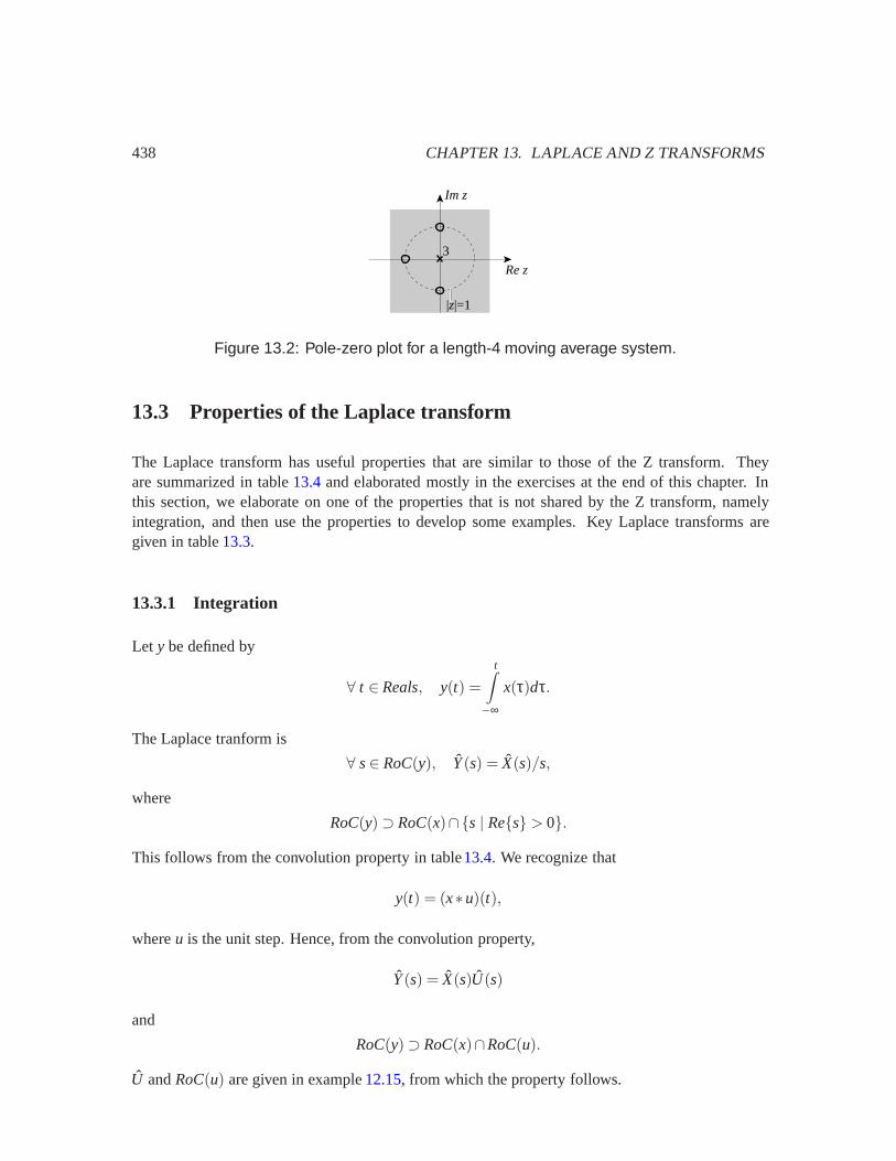
The (z−1) factors in the numerator and denominator cancel (fortunately, or we wouldhave a pole at z= 1, on the unit circle, and we would have to conclude that the systemwas unstable). A pole-zero plot is shown in figure 13.2.
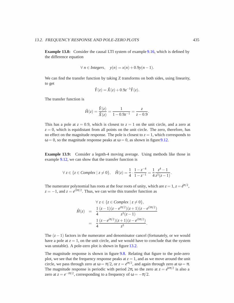
The magnitude response is shown in figure 9.8. Relating that figure to the pole-zeroplot, we see that the frequency response peaks at z= 1, and as we move around the unitcircle, we pass through zero at ω= π/2, or z= eiπ/2, and again through zero at ω= π.The magnitude response is periodic with period 2π, so the zero at z= e3iπ/2 is also azero at z= e−iπ/2, corresponding to a frequency of ω=−π/2.
436 CHAPTER 13. LAPLACE AND Z TRANSFORMS
Continuous-time signal∀ t ∈Reals
Laplace transform∀ s∈ RoC(x)
Roc(x) Reference
x(t) = δ(t− τ) X(s) = e−sτ Complex Exercise12.19
x(t) = u(t) X(s) = 1/s {s∈Complex| Re{s} > 0} Example12.15
x(t) = e−atu(t)
X(s) =1
s+a
{s∈Complex| Re{s} >−Re{a}}
Example12.18
x(t) =−e−atu(−t)
X(s) =1
s+a
{s∈Complex| Re{s} <−Re{a}}
Exercise 5
x(t) = cos(ω0t)u(t)X(s) =
s
s2 +ω20
{s | Re{s}> 0} Exercise 7
x(t) = sin(ω0t)u(t)X(s) =
ω0
s2 +ω20
{s | Re{s}> 0} Example13.10
x(t) =tN−1
(N−1)!e−atu(t) X(z) =
1(s+a)N
{s∈Complex| Re{s} >−Re{a}}
—
x(t) =− tN−1
(N−1)!e−atu(−t) X(z) =
1(s+a)N
{s∈Complex| Re{s} <−Re{a}}
—
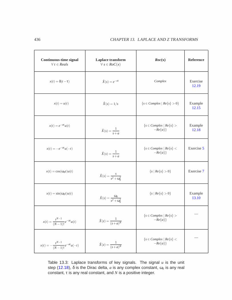
Table 13.3: Laplace transforms of key signals. The signal u is the unitstep (12.18), δ is the Dirac delta, a is any complex constant, ω0 is any realconstant, τ is any real constant, and N is a positive integer.

13.2. FREQUENCY RESPONSE AND POLE-ZERO PLOTS 437
Time domain∀ t ∈Reals
s domain∀ s∈RoC
RoC Name(reference)
w(t) = ax(t)+by(t) W(s) = aX(s)+bY(s) RoC(w)⊃ RoC(x)∩RoC(y) Linearity(exercise 6)
y(t) = x(t− τ) Y(s) = e−sτX(s) RoC(y) = RoC(x) Delay(exercise 7)
y(t) = (x∗h)(r) Y(s) = X(s)H(s) RoC(y)⊃RoC(x)∩RoC(h) Convolution(exercise 8)
y(t) = x∗(t) Y(s) = [X(s∗)]∗ RoC(y) = RoC(x) Conjugation(exercise 9)
y(t) = x(ct) Y(s) = X(s/c)/|c| RoC(y) ={s | s/c∈RoC(x)}
Time scaling(exercise 10)
y(t) = tx(t)
Y(s) =− dds
X(s)
RoC(y) = RoC(x) Scaling by t—
y(t) = eatx(t) Y(s) = X(s−a) RoC(y) ={s | s−a∈ RoC(x)}
Exponentialscaling
(exercise 11)
y(t) =t∫−∞
x(τ)dτ Y(s) = X(s)/s RoC(y)⊃RoC(x)∩{s | Re{s}> 0}
Integration(section 13.3.1)
y(t) =ddt
x(t)Y(s) = sX(s) RoC(y)⊃ RoC(x) Differentiation
(page 44)
Table 13.4: Properties of the Laplace transform. In this table, a,b are com-plex constants, c and τ are real constants.
438 CHAPTER 13. LAPLACE AND Z TRANSFORMS
|z|=1
Re z
Im z
3
Figure 13.2: Pole-zero plot for a length-4 moving average system.
13.3 Properties of the Laplace transform
The Laplace transform has useful properties that are similar to those of the Z transform. Theyare summarized in table 13.4 and elaborated mostly in the exercises at the end of this chapter. Inthis section, we elaborate on one of the properties that is not shared by the Z transform, namelyintegration, and then use the properties to develop some examples. Key Laplace transforms aregiven in table 13.3.
13.3.1 Integration
Let y be defined by
∀ t ∈Reals, y(t) =t∫
−∞
x(τ)dτ.
The Laplace tranform is
∀ s∈ RoC(y), Y(s) = X(s)/s,
where
RoC(y)⊃ RoC(x)∩{s | Re{s} > 0}.
This follows from the convolution property in table13.4. We recognize that
y(t) = (x∗u)(t),
where u is the unit step. Hence, from the convolution property,
Y(s) = X(s)U(s)
and
RoC(y)⊃ RoC(x)∩RoC(u).
U and RoC(u) are given in example 12.15, from which the property follows.
13.3. PROPERTIES OF THE LAPLACE TRANSFORM 439
Im s
Re s
RoC
s = iω
s = − iω
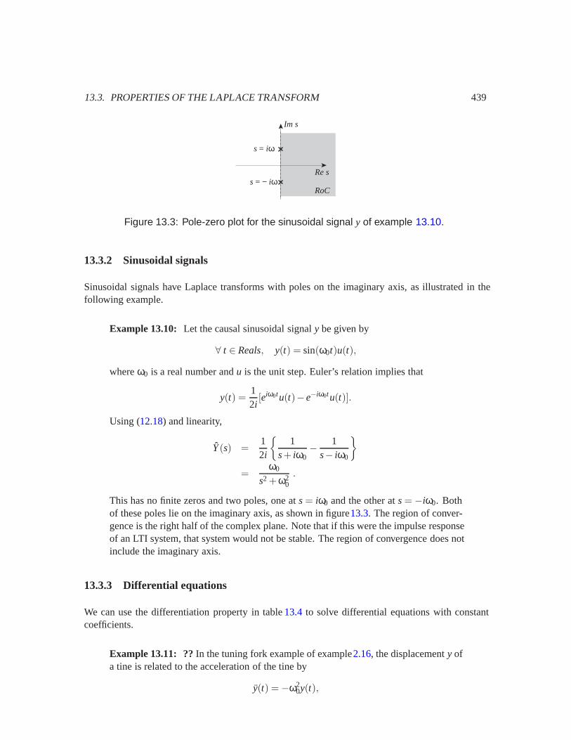
Figure 13.3: Pole-zero plot for the sinusoidal signal y of example 13.10.
13.3.2 Sinusoidal signals
Sinusoidal signals have Laplace transforms with poles on the imaginary axis, as illustrated in thefollowing example.
Example 13.10: Let the causal sinusoidal signal y be given by
∀ t ∈ Reals, y(t) = sin(ω0t)u(t),
where ω0 is a real number and u is the unit step. Euler’s relation implies that
y(t) =12i
[eiω0tu(t)−e−iω0tu(t)].
Using (12.18) and linearity,
Y(s) =12i
{1
s+ iω0− 1
s− iω0
}=
ω0
s2 +ω20
.
This has no finite zeros and two poles, one at s= iω0 and the other at s= −iω0. Bothof these poles lie on the imaginary axis, as shown in figure13.3. The region of conver-gence is the right half of the complex plane. Note that if this were the impulse responseof an LTI system, that system would not be stable. The region of convergence does notinclude the imaginary axis.
13.3.3 Differential equations
We can use the differentiation property in table 13.4 to solve differential equations with constantcoefficients.
Example 13.11: ?? In the tuning fork example of example2.16, the displacement y ofa tine is related to the acceleration of the tine by
y(t) =−ω20y(t),
440 CHAPTER 13. LAPLACE AND Z TRANSFORMS
where ω0 is a real constant. Let us assume that the tuning fork is initially at rest, and anexternal input x (representing say, a hammer strike) adds to the acceleration as follows,
y(t) =−ω20y(t)+x(t).
We can use Laplace transforms to find the impulse response of this LTI system. TakingLaplace transforms on both sides, using linearity and the differentiation property,
∀ s∈ RoC(y)∩RoC(x), s2Y(s) =−ω20Y(s)+ X(s).
From this, we can find the transfer function of the system,
H(s) =Y(s)X(s)
=1
s2 +ω20
.
Comparing this with example 13.10, we see that this differs only by a scaling by ω0
from the Laplace transform in that example. Thus, the pole-zero plot of the tuning forkis shown in figure 13.3, and the impulse response is given by
∀ t ∈ Reals, h(t) = sin(ω0t)u(t)/ω0.
Interestingly, this implies that the tuning fork is not stable. This impulse response isnot absolutely integrable. However, this model of the tuning fork is idealized. It failsto account for loss of energy due to friction. A more accurate model would be stable.
The above example can be easily generalized to find the transfer function of any LTI system de-scribed by a differential equation. In fact, Laplace transforms offer a powerful and effective way tosolve differential equations.
In the previous example, we inverted the Laplace transform by recognizing that it matched theexample before that. In the next chapter, we will give a more general method for inverting a Laplacetransform.
13.4 Frequency response and pole-zero plots, continuous time
Just as with Z transforms, the pole-zero plot of a Laplace transform can be used to get a quickestimate of key properties of an LTI system. Consider a stable continuous-time LTI system withimpulse response h, frequency response H , and rational transfer function H. We know that thefrequency response and transfer function are related by
∀ω∈ Reals, H(ω) = H(iω).
That is, the frequency response is equal to the Laplace transform evaluated on the imaginary axis.The imaginary axis is in the region of convergence because the system is stable.
Assume that H is a rational polynomial, in which case we can express it in terms of the first-orderfactors of the numerator and denominator polynomials,
H(s) =(s−q1) · · · (s−qM)(s− p1) · · · (s− pN)
,

13.4. FREQUENCY RESPONSE AND POLE-ZERO PLOTS, CONTINUOUS TIME 441
with zeros at q1, · · · ,qM and poles at p1, · · · , pN. The zeros and poles may be repeated (i.e., they mayhave multiplicity greater than one). The frequency response is therefore
∀ ω∈ Reals, H(ω) =(iω−q1) · · · (iω−qM)(iω− p1) · · · (iω− pN)
.
The magnitude response is
∀ ω∈ Reals, |H(ω)|= |iω−q1| · · · |iω−qM||iω− p1| · · · |iω− pN| .
Each of these factors has the form|iω−b|
where b is the location of either a pole or a zero. The factor |iω−b| is just the distance from iω tob in the complex plane.
Of course, iω is a point on the imaginary axis. If that point is close to a zero at location q, then thefactor |iω−q| is small, so the magnitude response will be small. If that point is close to a pole at p,then the factor |iω− p| is small, but since this factor is in the denominator, the magnitude responsewill be large. Thus,
The magnitude response of a stable LTI system may be estimated from the pole-zero plot of its transfer function. Starting at iω= 0, trace upwards and downwardsalong the imaginary axis to increase or decrease ω. If you pass near a zero, thenthe magnitude response should dip. If you pass near a pole, then the magnituderesponse should rise.
Example 13.12: Consider an LTI system with transfer function given by
∀ s∈ {s | Re{s} > Re{a}}, H(s) =s
(s−a)(s−a∗).
Suppose that a = c+ iω0. Figure 13.4 shows three pole-zero plots for ω0 = 1 andthree values of c, namely c = −1, c = −0.5, and c = −0.1. The magnitude frequencyresponses can be calculated and plotted using the following Matlab code:
omega = [-10:0.05:10];a1 = -1.0 + i;H1 = i*omega./((i*omega - a1).*(i*omega-conj(a1)));a2 = -0.5 + i;H2 = i*omega./((i*omega - a2).*(i*omega-conj(a2)));a3 = -0.1 + i;H3 = i*omega./((i*omega - a3).*(i*omega-conj(a3)));plot(omega, abs(H1), omega, abs(H2), omega, abs(H3));
The plots are shown together at the bottom of figure 13.4. The plot with the higherpeaks corresponds to the pole-zero plot with the poles closer to the imaginary axis.
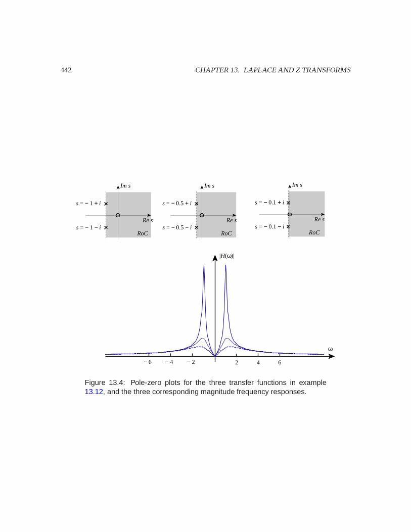
442 CHAPTER 13. LAPLACE AND Z TRANSFORMS
Im s
Re s
RoC
s = − 1 + i
2 4 6− 2− 4− 6
ω
|H(ω)|
s = − 1 − i
Im s
Re s
RoC
s = − 0.5 + i
s = − 0.5 − i
Im s
Re s
RoC
s = − 0.1 + i
s = − 0.1 − i
Figure 13.4: Pole-zero plots for the three transfer functions in example13.12, and the three corresponding magnitude frequency responses.
13.5. THE INVERSE TRANSFORMS 443
13.5 The inverse transforms
There are two inverse transforms. The inverse Z transform recovers the discrete-time signal x fromits Z transform X. The inverse Laplace transform recovers the continuous-time signal x from itsLaplace transform X. We study the inverse Z transform in detail. The inverse Laplace transform isalmost identical. The general approach is to break down a complicated rational polynomial into asum of simple rational polynomials whose inverse transforms we recognize. We consider only thecase where X can be expressed as a rational polynomial.
13.5.1 Inverse Z transform
The procedure is to construct the partial fraction expansion ofX, which breaks it down into a sumof simpler rational polynomials.
Example 13.13: Consider a Z transform given by
∀ z∈RoC(x), X(z) =1
(z−1)(z−2)=−1
z−1+
1z−2
. (13.6)
This sum is called the partial fraction expansion of X, and we will see below how tofind it systematically. We can write this as
∀ z∈ RoC(x), X(z) = X1(z)+ X2(z),
where X1(z) =−1/(z−1) and X2(z) = 1/(z−2) are the two terms.
To determine the inverse Z transforms of the two terms, we need to know their regionsof convergence. Recall from the linearity property that RoC(x) includes the intersectionof the regions of convergence of the two terms,
RoC(x) ⊃ RoC(x1)∩RoC(x2). (13.7)
Once we know these two regions of convergence, we can use table 13.1 to obtain theinverse Z transform of each term. By the linearity property the sum of these inverses isthe inverse Z transform of X.
X given by (13.6) has one pole at z= 1 and one pole at z= 2. From section 12.2.3 weknow that RoC(x) is bordered by these poles, so it has one of three forms:
1. RoC(x) = {z∈ Complex| |z|< 1},2. RoC(x) = {z∈ Complex| 1 < |z|< 2}, or
3. RoC(x) = {z∈ Complex| |z|> 2}.Suppose we have case (1), which implies that x is anti-causal. From (13.7), the regionof convergence of the term −1/(z− 1) must be {z∈ Complex| |z| < 1}. The onlyother possibility is {z∈ Complex| |z| > 1}, which would violate (13.7) unless theintersection is empty (which would not be an interesting case). Thus, from table13.1,

444 CHAPTER 13. LAPLACE AND Z TRANSFORMS
the inverse Z transform of the first term must be the anti-causal signal x1(n) = u(−n),for all n∈ Integers.
For the second term, 1/(z−2), its region of convergence could be either {z∈Complex| |z|<2} or {z∈ Complex| |z| > 2}. Again, the second possibility would violate (13.7), sowe must have the first possibility. This results in x2(n) = −2n−1u(−n), from the lastentry in table 13.1. Hence, the inverse Z transform is
∀ n∈ Integers, x(n) = u(−n)−2n−1u(−n).
If RoC(x) is given by case (2), we rewrite (13.6) slightly as
X(z) =−z−1 zz−1
+1
z−2.
The inverse Z transform of the first term is obtained from table 13.1, together with thedelay property in table 13.2. The inverse Z transform of the second term is the same asin case (1). We conclude that in case (2) the inverse Z transform is the two-sided signal
∀n, x(n) =−u(n−1)−2n−1u(−n).
In case (3), we write (13.6) as
X(z) =−z−1 zz−1
+z−1 zz−2
,
and conclude that the inverse Z transform is the causal signal
∀n, x(n) =−u(n−1)+ 2n−1u(n−1).
We can generalize this example. Consider any strictly proper rational polynomial
X(z) =A(z)B(z)
=aMzM + · · ·+a1z+a0
zN +bN−1zN−1 + · · ·+b1z+b0.
The numerator is of order M, the denominator is of order N. ‘Strictly proper’ means that M < N.We can factor the denominator,
X(z) =aMzM + · · ·+a1z+a0
(z− p1)m1(z− p2)m2 · · · (z− pk)mk. (13.8)
Thus X has k distinct poles at pi , each with multiplicy mi . Since the order of the denominator is N,it must be true that
N =k
∑i=1
mi . (13.9)
The partial fraction expansion of (13.8) is
X(z) =k
∑i=1
[Ri1
(z− pi)+
Ri2
(z− pi)2 + · · ·+ Rimi
(z− pi)mi
]. (13.10)

13.5. THE INVERSE TRANSFORMS 445
A pole with multiplicity mi contributes mi terms to the partial fraction expansion, so the total numberof terms is N, the order of the denominator, from (13.9). The coefficients Ri j are complex numberscalled the residues of the pole pi .
We assume that the poles p1, · · · , pN are indexed so that |p1| ≤ · · · |pN|. The RoC(x) must have oneof the following three forms:
1. RoC= {z∈ Complex| |z|< |p1|},2. RoC= {z∈ Complex| |pj−1|< |z|< |pj |}, for j ∈ {2, · · · ,k}, or
3. RoC= {z∈ Complex| |z|> |pk|} .
As in example 13.13, each term in the partial fraction expansion has two possible regions of conver-gence, only one of which overlaps with RoC(x). Thus, if we know RoC(x), we can determine theregion of convergence of each term of the partial fraction expansion, and then use table13.1 to findits inverse.
The following example illustrates how to find the residues.
Example 13.14: We will find the inverse Z transform of
X(z) =2z+ 3
(z−1)(z+ 2)=
R1
z−1+
R2
z+ 2.
The residues R1,R2 can be found by matching coefficients on both sides. Rewrite theright-hand side as
(R1 +R2)z+(2R1−R2)(z−1)(z+ 2)
.
Matching the coefficients of the numerator polynomials on both sides we conclude thatR1 +R2 = 2 and 2R1−R2 = 3. We can solve these simultaneous equations to determinethat R1 = 5/3 and R2 = 1/3.
Alternatively, we can find residue R1 by multiplying both sides by (z−1) and evaluatingat z= 1. That is,
R1 =2z+ 3z+ 2
∣∣∣∣z=1
=53.
Similarly, we can find R2 by we multiplying both sides by z+ 2 and evaluating atz=−2, to get
2z+ 3z−1
|z=−2 = R2,
so R2 = 1/3. Thus the partial fraction expansion is
X(z) =5/3z−1
+1/3z+ 2
.
RoC(x) is either
1. {z∈ Complex| |z|< 1},

446 CHAPTER 13. LAPLACE AND Z TRANSFORMS
2. {z∈ Complex| 1 < |z|< 2}, or
3. {z∈ Complex| |z|> 2}.Knowing which case holds, we can find the inverse Z transform of each term from table13.1. In the first case, x is the anti-causal signal
∀n, x(n) =−53
u(−n)− 13(−2)n−1u(−n).
In the second case it is the two-sided signal
∀n, x(n) =53
u(n−1)− 13(−2)n−1u(−n).
In the third case it is the causal signal
∀n, x(n) =53
u(n−1)+13(−2)n−1u(n−1).
If some pole of X has multiplicity greater than one, it is slightly more difficult to carry out the partialfraction expansion. The following example illustrates the method.
Example 13.15: Consider the expansion
X(z) =2z+ 3
(z−1)(z+ 2)2 =R1
z−1+
R21
z+ 2+
R22
(z+ 2)2 .
Again we can match coefficients and determine the residues. Alternatively, to obtainR1 we multiply both sides by (z− 1) and evaluate the result at z= 1, to get R1 = 5/9.To obtain R22 we multiply both sides by (z+ 2)2 and evaluate the result at z= −2, toget R22 = 1/3.
To obtain R21 we multiply both sides by (z+ 2)2,
2z+ 3z−1
=(z+ 2)2R1
z−1+R21(z+ 2)+R22,
and then differentiate both sides with respect to z. We evaluate the result at z= −2, toget
ddz
2z+ 3z−1
∣∣∣∣z=−2
= R21.
Hence R21 =−5/9. So the partial fraction expansion is
2z+ 3(z−1)(z+ 2)2 =
5/9z−1
− 5/9z+ 2
+1/3
(z+ 2)2 .
Knowing the RoC, we can now obtain the inverse Z transform ofX. For instance, in thecase where RoC= {z∈Complex| |z|> 2}, the inverse Z transform is the causal signal
∀n, x(n) =59
u(n−1)− 59(−2)n−1u(n−1)+
13(n−1)(−2)n−2u(n−2).
13.5. THE INVERSE TRANSFORMS 447
In example 13.15, we used the next to the last entry in table 13.1 to find the inverse transform ofthe term (1/3)/(z+ 2)2. That entry in the table is based on a generalization of the geometric seriesidentity, given by (12.9). The first generalization is
∞
∑n=0
(n+ 1)an = (∞
∑n=0
an)2 =1
(1−a)2 . (13.11)
The series above converges for any complex number a with |a| < 1 (see exercise3 of chapter 12).The broader generalization, for any integer k≥ 1, is
1k!
∞
∑n=0
(n+k)(n+k−1) · · · (n+ 1)an =1
(1−a)k+1 , (13.12)
for any complex number a with |a|< 1.
Consider then a Z transform X that has a pole at p of multiplicity m and no zeros. Since the pole pcannot belong to RoC, the RoCis either
{z∈ Complex| |z|> |p|} or {z∈ Complex| |z|< |p|}.
In the first case we expand X in a series involving only the terms z−n,n≥ 0,
X(z) =1
(z− p)m
=z−m
(1− pz−1)m
= z−m 1(m−1)!
∞
∑n=0
(m+n−1) · · ·(n+ 1)(pz−1)n, using (13.12)
=1
(m−1)!
∞
∑k=m
(k−1) · · · (k−m+ 1)pk−mz−k, defining k = n+m,
and the series converges for any z with |z| > |p|. We can match the coefficients of the powers of zin the Z transform definition,
X(z) =∞
∑k=−∞
x(k)z−k,
from which we can recognize that
∀k∈ Integers, x(k) =
{0, k < m
1(m−1)!(k−1) · · · (k−m+ 1)pk−m, k≥m
=1
(m−1)!(k−1) · · · (k−m+ 1)pk−mu(k−m). (13.13)
In the second case, RoC= {z∈ Complex| |z| < |p|}, we expand X in a series involving only theterms z−n,n≤ 0,
X(z) =1
(z− p)m
448 CHAPTER 13. LAPLACE AND Z TRANSFORMS
=1
(−p)m
1(1− p−1z)m
=1
(−p)m
1(m−1)!
∞
∑n=0
(m+n−1) · · ·(n+ 1)(p−1z)n, using (13.12)
=(−1)m
(m−1)!
0
∑k=−∞
(m−k−1) · · ·(1−k)pk−mz−k, defining k =−n,
and the series converges for any z with |z| < |p|. Again, we match powers of z in the Z transformdefinition to get
∀k∈ Integers, x(k) =
{(−1)m
(m−1)!(m−1−k) · · ·(1−k)pk−m, k≤ 0
0, k > 0
=(−1)m
(m−1)!(m−1−k) · · ·(1−k)pk−mu(−k). (13.14)
Example 13.16: Suppose
X(z) =1
(z−2)2
with RoC= {z∈ Complex| |z| > 2}. Then, by (13.13), X is the Z transform of thesignal
∀k∈ Integers, x(k) ={
0, k < 2(k−1)2k−2, k≥ 2
.
Suppose
Y(z) =1
(z−2)2
with RoC= {z∈ Complex| |z| < 2}. Then, by (13.14), Y is the Z transform of thesignal
∀k∈ Integers, y(k) ={
(1−k)2k−2, k≤ 00, k > 0
.
Since the unit circle {z∈Complex| |z|= 1} ⊂RoC, the DTFT of y is defined and givenby
∀ω∈ Reals, Y(ω) = Y(eiω) =1
(eiω−2)2 .
Now that we know how to inverse transform all the terms of the partial fraction expansion, we cangeneralize the method used in example 13.15 to calculate the inverse Z transform of any X of theform
X(z) =aMzM + · · ·+a0
zN +bN−1zN−1 + · · ·+b0.
Step 1 If M ≥ N, divide through to obtain
X(z) = cM−NzM−N + · · ·+c0 +W(z),

13.5. THE INVERSE TRANSFORMS 449
where W is strictly proper.
Step 2 Carry out the partial fraction expansion ofW and, knowing the RoC, obtain the inverse Ztransform w. Then from table 13.1,
∀n, x(n) = cm+l−Nδ(n+m+ l−N)+ · · ·+c0δ(n)+w(n).
Example 13.17: We follow the procedure for
X(z) =z2 +z+ 1+z−1
(z+ 2)2 .
First, to get this into the proper form, as a rational polynomial in z, notice that
X(z) = z−1Y(z),
where
Y(z) =z3 +z2 +z+ 1
(z+ 2)2 .
Since z−1 corresponds to a one-step delay,
x(n) = y(n−1),
so if we find the inverse Z transform of Y, then we have found the inverse Z trasformof X.
Working now with Y, step 1 yields
Y(z) = z−3+9z+ 13
z2 + 4z+ 4.
Step 2 gives
W(z) =9z+ 13(z+ 2)2 =
−5(z+ 2)2 +
9z+ 2
.
Suppose RoC= {z∈ Complex| |z|> 2}. Then from table 13.1,
∀n, w(n) = −5(n−1)(−2)n−2u(n−2)+ 9(−2)n−1u(n−1),∀n, y(n) = δ(n+ 1)−3δ(n)+w(n),∀n, x(n) = y(n−1).
Hence, for all n∈ Integers,
x(n) = δ(n)−3δ(n−1)−5(n−2)(−2)n−3u(n−3)+ 9(−2)n−2u(n−2).
450 CHAPTER 13. LAPLACE AND Z TRANSFORMS
13.5.2 Inverse Laplace transform
The procedure to calculate the inverse Laplace transform is virtually identical. Suppose the Laplacetransform X is a rational polynomial
X(s) =aMsM + · · ·+a0
sN +bN−1sN−1 + · · ·+b0.
We follow Steps 1 and 2 above. We divide through in case M ≥ N to obtain
X(s) = cM−NsM−N + · · ·+c0 +W(s),
where W is strictly proper. We carry out the partial fraction expansion ofW. Knowing RoC(x),we can again infer the region of convergence of each term. We then obtain the inverse Laplacetransform term by term using table 13.3,
∀t ∈ Reals, x(t) = cm−nδ(M−N)(t)+ · · ·+c0δ(t)+w(t).
Here w is the inverse Laplace transform of W, δ is the Dirac delta function, and δ(i) is the ithderivative of the Dirac delta function.1
Example 13.18: We follow the procedure and obtain the partial fraction expansion of
X(s) =s3 +s2 +s+ 1
s(s+ 2)2
= 1+−3s2−3s+ 1
s(s+ 2)2
= 1+1/4s
+−13/4s+ 2
+5/2
(s+ 2)2 .
X has one pole at s= 0 and a pole at s=−2 of multiplicity two. So its RoChas one ofthree forms:
1. RoC= {s∈ Complex| Re{s}<−2},2. RoC= {s∈ Complex| −2 < Re{s} < 0}, or
3. RoC= {s∈ Complex| Re{s}> 0}.We now use table 13.3 to obtain the inverse Laplace transform of each term. In case(1), the continuous-time signal is the anti-causal signal
∀ t, x(t) = δ(t)− 14
u(−t)+134
e−2tu(−t)− 52
te−2tu(−t).
In case (2), it is the two-sided signal,
∀t, x(t) = δ(t)− 14
u(−t)− 134
e−2tu(t)+52
te−2tu(t).
In case (3), it is the causal signal,
∀t, x(t) = δ(t)+14
u(t)− 134
e−2tu(t)+52
te−2tu(t).
1The derivative of δ is a function only in a formal sense, and we obtain its Laplace transform using the differentiationproperty in table 13.4.
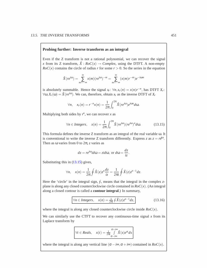
13.5. THE INVERSE TRANSFORMS 451
Probing further: Inverse transform as an integral
Even if the Z transform is not a rational polynomial, we can recover the signalx from its Z transform, X : RoC(x) → Complex, using the DTFT. A non-emptyRoC(x) contains the circle of radius r for some r > 0. So the series in the equation
X(reiω) =∞
∑m=−∞
x(m)(reiω)−m =∞
∑m=−∞
(x(m)r−m)e−iωm
is absolutely summable. Hence the signal xr : ∀n,xr(n) = x(n)r−n, has DTFT Xr :∀ω,Xr(ω) = X(reiω). We can, therefore, obtain xr as the inverse DTFT of Xr
∀n, xr(n) = r−nx(n) =1
2π
∫ 2π
0X(reiω)eiωndω.
Multiplying both sides by rn, we can recover x as
∀n∈ Integers, x(n) =1
2π
∫ 2π
0X(reiω)(reiω)ndω. (13.15)
This formula defines the inverse Z transform as an integral of the real variable ω. Itis conventional to write the inverse Z transform differently. Express z as z= reiω.Then as ω varies from 0 to 2π, z varies as
dz= reiωidω= zidω, or dω=dziz
.
Substituting this in (13.15) gives,
∀n, x(n) =1
2π
∮X(z)zn dz
iz=
12πi
∮X(z)zn−1dz.
Here the ‘circle’ in the integral sign,∮
, means that the integral in the complex z-plane is along any closed counterclockwise circle contained in RoC(x). (An integralalong a closed contour is called a contour integral.) In summary,
∀n∈ Integers, x(n) = 12πi
∮X(z)zn−1dz, (13.16)
where the integral is along any closed counterclockwise circle inside RoC(x).
We can similarly use the CTFT to recover any continuous-time signal x from itsLaplace transform by
∀t ∈ Reals, x(t) = 12πi
σ+i∞∫σ−i∞
X(s)estds
where the integral is along any vertical line (σ− i∞,σ+ i∞) contained in RoC(x).

452 CHAPTER 13. LAPLACE AND Z TRANSFORMS
Probing further: Differentiation property of the Laplace transform
We can use the inverse Laplace transform as given in the box on page451 to demon-strate the differentiation property in table 13.4. Let y be defined by
∀ t ∈ Reals, y(t) =ddt
x(t).
We can write x in terms of its Laplace transform as
∀t ∈ Reals, x(t) =1
2πi
∫ σ+i∞
σ−i∞X(s)estds.
Differentiating this with respect to t is easy,
∀t ∈ Reals,ddt
x(t) =1
2πi
∫ σ+i∞
σ−i∞sX(s)estds.
Consequently, y(t) = dx(t)/dt is the inverse transform of sX(s), so
∀ s∈ RoC(y), Y(s) = sX(s),
where RoC(y) ⊃RoC(x).
13.6 Steady state response
Although it has been a fair amount of work, being able to compute an inverse transform for anarbitrary rational polynomial proves useful. Our first use will be to study the stead-state responseof a causal and stable LTI system that has a sinusoidal input that starts at time zero.
If the input to an LTI system is a complex exponential,
∀t ∈ Reals, x(t) = eiωt ,
then the output y is an exponential of the same frequency but with amplitude and phase given byH(ω),
∀t ∈ Reals, y(t) = H(ω)eiωt ,
where H is the frequency response. However, this result requires the exponential input to start att = −∞. In practice, of course, an input may start at some finite time, say at t = 0, but this resultdoes not describe the output if the input is
∀t ∈Reals, x(t) = eiωtu(t). (13.17)
We will see that if the system is stable and causal,2 then the output y decomposes into two parts, a
2This result can be generalized to non-causal systems, but causal systems will be sufficient for our purposes.
13.6. STEADY STATE RESPONSE 453
transient output and a steady state output,
y = ytr +yss,
where the transient becomes vanishingly small for large t. That is,
limt→∞
ytr(t) = 0.
Moreover, the steady state signal is the exponential,
∀t, yss(t) = H(ω)eiωtu(t). (13.18)
Thus for stable systems, we can use the frequency response to describe the eventual output to sinu-soidal signals that start at some finite time.
For the special case ω= 0, the input (13.17) is the unit step, x = u, and yss= H(0)u. So for stablesystems, the steady state response to a unit step input is a step of size H(0). (H(0) is called the dcgain.) This case is important in the design of feedback control, considered in the next chapter.
Let h be the impulse response and H be the Laplace transform of a stable and causal LTI system.We assume for simplicity that H is a strictly proper rational polynomial all of whose poles havemultiplicity one,
H(s) =A(s)
(s− p1) · · · (s− pN).
Because the system is causal, RoC(h) has the form
RoC(h) = {s | Re{s} > q},where q is the largest real part of any pole. Since the system is stable, q < 0, so that the region ofconvergence includes the imaginary axis.
From table 13.3 the Laplace transform X of the signal (13.17) is
X(s) =1
s− iω,
with RoC(x) = {s∈ Complex| Re{s} > 0}.The Laplace transform of the output y = h∗x is
Y = HX,
withRoC(y)⊃RoC(h)∩RoC(x) = {s∈ Complex| Re{s}> 0}.
The partial fraction expansion ofY is
Y(s) = H(s)X(s) =A(s)
(s− p1) · · · (s− pN)· 1s− iω
(13.19)
=R1
s− p1+ · · ·+ RN
s− pN+
Rω
s− iω. (13.20)
454 CHAPTER 13. LAPLACE AND Z TRANSFORMS
Because everything is causal, each term must be causal, so from table13.3 we obtain
∀t, y(t) =N
∑k=1
Rkepktu(t)+Rωeiωtu(t).
We decompose y = ytr +yss, with
∀t, ytr(t) =N
∑k=1
Rkepktu(t),
∀t, yss(t) = Rωeiωtu(t).
Since Re{pk}< 0 for k = 1, · · · ,N,limt→∞
ytr(t) = 0.
Thus, the steady-state response yss is eventually all that is left.
Finally, the residue Rω is obtained by multiplying both sides of (13.19) by s− iω and evaluating ats= iω to get Rω = H(iω) = H(ω), so that
∀t, yss(t) = H(ω)eiωtu(t).
This analysis reveals several interesting features of the total response y. First, from (13.20) we seethe poles p1, · · · , pN of the transfer function contribute to the transient response ytr , and the pole ofthe input X at iω contributes to the steady state response. Second we can determine how quickly thetransient response dies down. The transient response is
∀t, ytr(t) = R1ep1tu(t)+ · · ·+RNepNtu(t).
The magnitude of the terms is
|R1|eRe{p1}t , · · · , |RN|eRe{pN}t .
Each term decreases exponentially with t, since the real parts of the poles are negative. The slowestdecrease is due to the pole with the least negative part. Thus the pole of the stable, causal transferfunction with the least negative part determines how fast the transient response goes to zero. Indeedfor large t, we can approximate the response y as
y(t) ≈ Riepit +H(ω)eiωt ,
where pi is the pole with the largest (least negative) real part.
There is a similar result for discrete-time systems, and it is obtained in the same way. Suppose anexponential input
∀n∈ Integers, x(n) = eiωnu(n),
is applied to a stable and causal system with impulse response h, transfer functionH, and frequencyresponse H . Then the output y = h∗x can again be decomposed as
∀n, y(n) = ytr(n)+yss(n),
13.7. LINEAR DIFFERENCE AND DIFFERENTIAL EQUATIONS 455
where the transient ytr(n)→ 0 as n→ ∞, and the steady state response is
∀n, yss(n) = H(eiω)eiωnu(n) = H(ω)eiωnu(n).
For large n, the transient response decays exponentially as pni , i.e.
y(n)≈ Ri pni +yss(n),
where pi is the pole with the largest magnitude (which must be less than one, since the system isstable).
13.7 Linear difference and differential equations
Many natural and man-made systems can be modeled as linear differential equations or differenceequations. We have seen that when such systems are initially at rest, they are LTI systems. Hence,we can use their transfer functions (which are Z transforms or Laplace transforms) to analyze theresponse of these systems to external inputs.
However, physical systems are often not initially at rest. Dealing with non-zero initial conditionsintroduces some complexity in the analysis. Mathematicians call such systems with non-zero initialconditions initial value problems. We can adapt our methods to deal with initial conditions. Therest of this chapter is devoted to these methods.
Example 13.19: In example 13.8 we considered the LTI system described by thedifference equation
y(n)−0.9y(n−1) = x(n).
The transfer function of this system is H(z) = z/(z− 0.9). If the system is initially atrest, we can calculate its response y from its Z transformY = HX. For instance, if theinput is the unit step, X(z) = z/(z−1),
Y(z) =z2
(z−0.9)(z−1)=−9z
z−0.9+
10zz−1
,
and so y(n) =−9(0.9)n + 10,n≥ 0.
We cannot use the transfer function, however, to determine the response if the initialcondition at time n= 0 is y(−1) = y(−1), and the input is x(n) = 0,n≥ 0. The responseto this initial condition is
y(n) = y(−1)(0.9)n+1, n≥−1.
We can check that this expression is correct by verifying that it satisfies both the initialcondition and the difference equation.
If the initial condition is y(−1) = y(−1) and the input is a unit step, the response turnsout to be the sum of the response due to the input (with zero initial condition) and theresponse due to the initial condition (with zero input),
y(n) = [−9(0.9)n + 10]+ [y(−1)(0.9)n+1], n≥ 0.
456 CHAPTER 13. LAPLACE AND Z TRANSFORMS
For small values of n the response depends heavily on the initial condition, especiallyif y(0) is large. Because this system is stable, the effect of the initial condition becomesvanishingly small for large n.
An LTI difference equation has the form
y(n)+a1y(n−1)+ · · ·+amy(n−m) = b0x(n)+ · · ·+bkx(n−k), n≥ 0. (13.21)
We interpret this equation as describing a causal discrete-time LTI system in which x(n) is the inputand y(n) is the output at time n. The ai and bj are constant coefficients that specify the system.
We have used difference equations before. In section 8.2.1 we used this form and the discrete timeFourier transform to find the frequency response of this system. In section 9.5 we showed howto realize such systems as IIR filters. In example 13.19 we used the transfer function to find theresponse. But in all these cases, we had to assume that the system was initially at rest. We nowdevelop a method to find the response for arbitrary inital conditions.
We assume the input signal x starts at some finite time, which we take to be zero, x(n) = 0,n< 0. Wewish to calculate y(n),n≥ 0. From (13.21) we can see that we need to be given m initial conditions,
y(−1) = y(−1), · · · ,y(−m) = y(−m).
Given the input signal and these initial conditions, there is a straightforward procedure to calculatethe output response y(n),n≥ 0: Rewrite (13.21) as
y(n) =−a1y(n−1)−·· ·−amy(n−m)+b0x(n)+ · · ·+bkx(n−k), (13.22)
and recursively use (13.22) to obtain y(0),y(1),y(2), · · ·. For n = 0, (13.22) yields
y(0) = −a1y(−1)−·· ·−amy(−m)+b0x(0)+ · · ·+bkx(−k)= −a1y(−1)−·· ·−amy(−m)+b0x(0).
All the terms on the right are known from the initial conditions and the input x(0), so we cancalculate y(0). Next, taking n = 1 in (13.22),
y(1) =−a1y(0)+ · · ·+amy(1−m)+b0x(1)+ · · ·+bkx(1−k).
All the terms on the right are known either from the given data or from precalculated values—y(0)in this case. Proceeding in this way we can calculate the remaining values of the output sequencey(2),y(3), · · ·, one at a time.
We now use the Z transform to calculate the entire output sequence. Multiplying both sides of(13.21) by u(n), the unit step, gives us a relation that holds among signals whose domain is Integers:
y(n)u(n)+a1y(n−1)u(n)+ · · ·+amy(n−m)u(n) = b0x(n)u(n)+ · · ·+bkx(n−k)u(n), n∈ Integers.
We can now take the Z transforms of both sides. We multiply both sides by z−n and sum,
∞
∑n=0
y(n)z−n+a1
∞
∑n=0
y(n−1)z−n+ · · ·+am
∞
∑n=0
y(n−m)z−n = b0
∞
∑n=0
x(n)z−n+ · · ·+bk
∞
∑n=0
x(n−k)z−n.
(13.23)
13.7. LINEAR DIFFERENCE AND DIFFERENTIAL EQUATIONS 457
Define
X(z) =∞
∑n=0
x(n)z−n, Y(z) =∞
∑n=0
y(n)z−n.
Each sum in (13.23) can be expressed in terms ofY or X. In evaluting the Z transforms of the signalsy(n−1)u(n),y(n−2)u(n), · · · we need to include the initial conditions:
∞
∑n=0
y(n−1)z−n = y(−1)z0 +z−1∞
∑n=1
y(n−1)z−(n−1) = y(−1)z0 +z−1Y(z),
∞
∑n=0
y(n−2)z−n = y(−2)z0 + y(−1)z−1 +z−2∞
∑n=2
y(n−2)z−(n−2)
= y(−2)z0 + y(−1)z−1 +z−2Y(z),· · ·
∞
∑n=0
y(n−m)z−n = y(−m)z0 + · · ·+ y(−1)z−(m−1) +z−m∞
∑n=m
y(n−m)z−(n−m)
= y(−m)z0 + · · ·+ y(−1)z−(m−1) +z−mY(z).
Because x(n) = 0,n < 0, by assumption, the sums on the right in (13.23) are simpler:
∞
∑n=0
x(n−1)z−n = x(−1)z0 +z−1X(z) = z−1X(z)
∞
∑n=0
x(n−2)z−n = x(−2)z0 +x(−1)z−1 +z−2X(z) = z−2X(z)
· · ·∞
∑n=0
x(n−k)z−n = x(−k)z0 + · · ·+x(−1)z−(k−1) +z−kX(z) = z−kX(z).
(If there were non-zero initial conditions for x(−1), · · · ,x(−k), we could include them in the Ztransforms of x(n−1)u(n), · · · ,x(n−k)u(n).) Substituting these relations in (13.23) yields
Y(z) + a1[z−1Y(z)+ y(−1)z0]+ · · ·+am[z−mY(z)+ y(−m)z0 + · · · y(−1)z−(m−1)]= b0X(z)+b1z−1X(z)+ · · ·bkXz−k, (13.24)
from which, by rearranging terms, we obtain
[1+a1z−1 + · · ·+amz−m]Y(z) = [b0 +b1z−1 + · · ·+bkz−k]X(z)+C(z),
where C(z) is an expression involving only the initial conditions y(−1), · · · , y(−m). Therefore,
Y(z) =b0 +b1z−1 + · · ·bkz−k
1+a1z−1 + · · ·+amz−mX(z)+
C(z)1+a1z−1 + · · ·+amz−m
.
We rewrite this relation as
Y(z) = H(z)X(z)+C(z)
1+a1z−1 + · · ·+amz−m. (13.25)
458 CHAPTER 13. LAPLACE AND Z TRANSFORMS
where
H(z) = b0+b1z−1+···+bkz−k
1+a1z−1+···+amz−m . (13.26)
Observe that if the initial conditions are all zero, C(z) = 0, and we only have the first term on theright in (13.25); and if the input is zero—i.e., x(n) = 0 for all n, then X(z) = 0, and we only havethe second term.
By definition, Y(z) is the Z transform of the causal signal y(n)u(n),n∈ Integers. So its RoC= {z∈Complex| |z| > |p|} in which p is the pole of the right side of (13.25) with the largest magnitude.The inverse Z transform of Y can be expressed as
∀n≥ 0, y(n) = yzs(n)+yzi(n), (13.27)
where yzs(n), the inverse Z transform of HX, is the zero-state response, and yzi(n), the inverse Ztransform of C(z)/[1 + a1z−1 + · · ·+ amz−m], is the zero-input response. The zero-state response,also called the forced response, is the output when all initial conditions are zero. The zero-inputresponse, also called the natural response, is the output when the input is zero.
Thus the (total) response is the sum of the zero-state and zero-input response. We first encounteredthis property of linearity in chapter 5.
By definition, the transfer function is the Z transform of the zero-state impulse response. TakingC = 0 and X = 1 in (13.25) shows that the transfer function is H(z). From (13.26) we see that Hcan be written down by inspection of the difference equation (13.21). If the system is stable—allpoles of H are inside the unit circle—the frequency response is
∀ω, H(ω) = H(eiω) =b0 +b1e−iω+ · · ·+bke−ikω
1+a1e−iω+ · · ·+ame−imω .
We saw this relation in (8.21).
Example 13.20: Consider the difference equation
y(n)− 56
y(n−1)+16
y(n−2) = x(n), n≥ 0.
Taking Z transforms as in (13.24) yields
Y(z)− 56[z−1Y(z)+ y(−1)]+
16[z−2Y(z)+ y(−2)+ y(−1)z−1] = X(z).
Therefore
Y(z) =1
1− 56z−1 + 1
6 z−2X(z)+
56 y(−1)+ 1
6 y(−2)+ 16 y(−1)z−1
1− 56z−1 + 1
6z−2
=z2
z2− 56 z+ 1
6
X(z)+[5
6 y(−1)+ 16 y(−2)]z2 + 1
6 y(−1)z
z2− 56z+ 1
6
,
from which we can obtain Y for a specified X and initial conditions y(−1), y(−2). Thetransfer function is
H(z) =z2
z2− 56z+ 1
6
=z2
(z− 13)(z− 1
2),
13.7. LINEAR DIFFERENCE AND DIFFERENTIAL EQUATIONS 459
which has poles at z= 1/3 and z= 1/2 (and two zeros at z= 0). The system is stable.The zero-state impulse response h is the inverse Z transform ofH(z), which we obtainusing partial fraction expansion,
H(z) = z
[−2
z− 13
+3
z− 12
]
so that
∀n∈ Integers, h(n) =−2
(13
)n
u(n)+ 3
(12
)n
u(n).
We can recognize that the impulse response consists of two terms, each contributed byone pole of the transfer function.
Suppose the initial conditions are y(−1) = 1, y(−2) = 1 and the input x is the unit step,so X(z) = z/(z−1). Then the zero-input response, yzi, has Z transform
Yzi(z) =[5
6 y(−1)+ 16 y(−2)]z2 + 1
6 y(−1)z(z− 1
3)(z− 12)
=z2 + 1
6z
(z− 13)(z− 1
2)= z
[−3
z− 13
+4
z− 12
],
so
∀n, yzi(n) =−3
(13
)n
u(n)+ 4
(12
)n
u(n).
The zero-state response, yzs, has Z transform
Yzs(z) = H(z)X(z) =z3
(z− 13 )(z− 1
2)(z−1)
= z
[1
z− 13
+−3
z− 12
+3
z−1
],
so
∀n, yzs(n) =(
13
)n
u(n)−3
(12
)n
u(n)+ 3u(n).
The (total) response
∀n∈ Integers, y(n) = yzs(n)+yzi(n) = 3u(n)+ [−2(1/3)n +(1/2)n]u(n),
can also be expressed as the sum of the steady-state and the transient response withyss(n) = 3u(n) and ytr(n) = −2(1/3)nu(n)+ (1/2)nu(n). Note that the decompositionof the response into the sum of the zero-state and zero-input responses is different fromits decomposition into the steady-state and transient responses.
460 CHAPTER 13. LAPLACE AND Z TRANSFORMS
13.7.1 LTI differential equations
The analogous development for continuous time concerns systems described by a LTI differentialequation of the form
dmydtm
(t)+am−1dm−1ydtm−1 (t)+ · · ·+a1
dydt
(t)+a0y(t) = bkdkxdtk
(t)+ · · ·+b1dxdt
(t)+b0x(t), t ≥ 0.
(13.28)We interpret this equation as describing a causal continuous-time LTI system in which x(t) is theinput and y(t) is the output at time t. The constant coefficients ai and bj specify the system.
In section 8.2.1 we used this form to find the frequency response. In example 13.11, we used theLaplace transform to find the transfer function of a tuning force. But in both cases, we assumed thatthe system was initially at rest. We now develop a method to find the response to arbitrary initialconditions. We begin with a simple circuit example.
Example 13.21: A series connection of a resistor R, a capacitor C, and a voltagesource x, is described by the differential equation
dydt
(t)+1
RCy(t) = x(t),
in which y is the voltage across the capacitor. The differential equation is obtained fromKirchhoff’s voltage law. The transfer function of this system isH(s) = 1/(s+ 1/RC).So if the system is initially at rest, we can calculate the response y from its Laplacetransform Y = HX. For instance, if the input is a unit step, X(s) = 1/s,
Y(s) =1
(s+ 1/RC)s=−RC
s+ 1/RC+
RCs
,
therefore, y(t) =−RCe−t/RC+RC, t ≥ 0.
We cannot use this transfer function, however, to determine the response if the initialcapacitor voltage is y(0) = y(0) and x(t) = 0, t ≥ 0. The response in this case is
y(t) = y(0)e−t/RC, t ≥ 0.
We can check that expression is correct by verifying that it satisfies the given initialcondition and the differential equation.
If the initial condition is y(0) = y(0) and the input is a unit step, the response turnsout to be the sum of the response due to the input (with zero initial condition) and theresponse due to the initial condition (with zero input),
y(t) = [−RCe−t/RC+RC]+ [y(0)e−t/RC], t ≥ 0.
For the general case (13.28) we assume that the input x starts at some finite time which we take tobe zero, so x(t) = 0, t < 0. We wish to calculate y(t), t ≥ 0. From the theory of differential equationswe know that we need to be given m initial conditions,
y(0) = y(0),dydt
(0) = y(1)(0), · · · , dm−1ydtm−1 (0) = y(m−1)(0),
13.7. LINEAR DIFFERENCE AND DIFFERENTIAL EQUATIONS 461
in order to calculate y(t), t ≥ 0.
Because time is continuous, there is no recursive procedure for calculating the output from the givendata as we did in (13.22). Instead we calculate the output signal using the Laplace transform. Wedefine the Laplace transforms of the signals y(t)u(t),y(1)(t)u(t), · · · ,y(m)(t)u(t),x(t)u(t):
Y(s) =∫ ∞
−∞y(t)u(t)e−stdt =
∫ ∞
0y(t)e−stdt
Y(i)(s) =∫ ∞
−∞y(i)(t)u(t) =
∫ ∞
0y(i)(t)e−stdt, i = 1, · · · ,m
X(s) =∫ ∞
−∞x(t)u(t)e−stdt =
∫ ∞
0x(t)e−stdt.
Here we use the notation y(i)(t) = ditdti y(t), t ≥ 0. We now derive the relations between these Laplace
transforms.
The derivative y(1)(t) = dydt (t) and y are related by
y(t)u(t) = y(0)u(t)+∫ t
0y(1)(τ)u(τ)dτ = y(0)u(t)+
∫ t
0y(1)(τ)u(τ)dτ, t ∈ Reals.
Using integration by parts,
Y(s) =∫ ∞
0y(t)e−stdt =
∫ ∞
0y(0)e−stdt +
∫ ∞
0
(∫ t
0y(1)(τ)dτ
)e−stdt
=1sy(0)− 1
s
∫ t
0y(1)(τ)dτe−st |∞t=0 +
1s
∫ ∞
0y(1)(t)e−stdt
=1s[Y(1)(s)+ y(0)].
Therefore,
Y(1)(s) = sY(s)− y(0). (13.29)
Repeating this procedure, we get the Laplace transforms of the higher-order derivatives,
Y(2)(s) = sY(1)(s)− y(1)(0)= s2Y(s)−sy(0)− y(1)(0)· · ·
Y(m)(s) = smY(s)−sm−1y(0)−sm−2y(1)(0)−·· ·− y(m−1)(0).
On the other hand, because x(i)(t) = dixdti (t) for all t ∈ Reals, using the differentiation property in
table 13.4, we obtain
X(1)(s) = sX(s)· · ·
X(k)(s) = skX(s).
462 CHAPTER 13. LAPLACE AND Z TRANSFORMS
By substituting from the relations just derived, we obtain the Laplace transforms of all the terms in(13.28),
[smY(s)−sm−1y(0)−·· ·− ym−1(0)]+am−1[sm−1Y(s)−sm−2y(0)−·· ·− ym−2(0)]· · ·+a1[sY(s)− y(0)]+a0Y(s) = bks
kX(s)+ · · ·+b1sX(s)+b0X(s). (13.30)
Rearranging terms yields
[sm+am−1sm−1 + · · ·+a1s+a0]Y(s) = [bksk + · · ·+b1s+b0]X(s)+C(s),
in which C is an expression involving only the intial conditions y(0), · · · , y(m−1)(0). Therefore,
Y(s) =bksk +bk−1sk−1 + · · ·b1s+b0
sm+am−1sm−1 + · · ·a1s+a0X(s)+
C(s)sm+am−1sm−1 + · · ·a1s+a0
, (13.31)
which we also write as
Y(s) = H(s)X(s)+C(s)
sm+am−1sm−1 + · · ·a1s+a0, (13.32)
in which
H(s) = bksk+···+b1s+b0sm+···+a1s+a0
. (13.33)
If the initial conditions are all zero,C(s) = 0, and we only have the first term on the right in (13.32);if the input is zero—i.e., x(t) = 0 for all t, then X(s) = 0, and we only get the second term in (13.32).
By definition, Y(s) is the Laplace transform of the causal signal y(t)u(t), t ∈ Reals. So its RoC={s∈ Complex| Re{s} > Re{p}}, where p is a pole of the right side of (13.32) with the largest realpart.
Taking the inverse Laplace transform ofY, we can decompose the output signal y as
∀t, y(t) = yzs(t)+yzi(t),
where yzs, the inverse Laplace transform of HX, is the zero-state or forced response and yzi, theinverse Laplace transform ofC(s)/[sm+ · · ·+a0], is the zero-input or natural response. The (total)response is the sum of the zero-state and zero-input response, which is a general property of linearsystems.
By definition, the transfer function is the Laplace transform of the zero-state impulse response.Taking C = 0 and X = 1 (the Laplace transform of the unit impulse) in (13.32) shows that thetransfer function is H(s) which, as we see from (13.33), can be written down by inspection of thedifferential equation (13.28). If the system is stable—all poles of H(s) have real parts strictly lessthan zero—the frequency response is
∀ω, H(ω) = H(iω) =bk(iω)k + · · ·+b1iω+b0
(iω)m+ · · ·+a1iω+a0.
We saw this relation in (??).
13.8. STATE-SPACE MODELS 463
Example 13.22: We find the response y(t), t ≥ 0, for the differential equation
d2ydt2
+ 3dydt
+ 2y = 3x(t)+dxdt
,
when the input is a unit step x(t) = u(t) and the initial conditions are y(0) = 1,y(1)(0) =2. Taking Laplace transforms of both sides as in (13.30),
[s2Y(s)−sy(0)− y(1)(0)]+ 3[sY(s)− y(0)]+ 2Y(s) = 3X(s)+sX(s).
Therefore,
Y(s) =s+ 3
s2 + 3s+ 2X(s)+
sy(0)+ y(1)(0)+ 3y(0)s2 + 3s+ 2
.
Substituting X(s) = 1/s, y(0) = 1, y(1) = 2, yields
Y(s) =s+ 3
s(s2 + 3s+ 2)+
s+ 5s2 + 3s+ 2
= [3/2
s− 2
s+ 1+
1/2s+ 2
]+ [4
s+ 1− 3
s+ 2].
Taking inverse Laplace transforms gives
∀t, y(t) = yzs(t)+yzi(t)
= [32
u(t)−2e−tu(t)+12
e−2tu(t)]+ [4e−tu(t)−3e−2tu(t)]
=32
u(t)+ [2e−t − 52
e−2t ]u(t)
= yss(t)+ytr(t).
As in the case of difference equations, the decomposition of the response into zero-state and zero-input responses is different from the decomposition into transient andsteady-state responses. (Indeed, the steady-state response does not exist if the systemis unstable, whereas the former decomposition always exists.)
13.8 State-space models
This section is mathematically more advanced in that it uses the operation of matrix inverse.
In section 5.3 we introduced single-input, single-output (SISO) multidimensional state-space mod-els of discrete-time and continuous-time LTI systems. For LTI systems, state-space models providean alternative description to difference or differential equation representations. The advantage ofstate-space models is that by using matrix notation we have a very compact representation of theresponse, independent of the order of the system. We develop a method that combines this matrixnotation with transform techniques to calculate the response.
The discrete-time SISO state-space model is
∀ n≥ 0, s(n+ 1) = As(n)+bx(n), (13.34)
y(n) = cTs(n)+dx(n), (13.35)
464 CHAPTER 13. LAPLACE AND Z TRANSFORMS
in which s(n) ∈ RealsN is the state, x(n) ∈ Realsis the input, and y(n) ∈ Realsis the output at timen. In this [A,b,c,d] representation, A is an N×N (square) matrix, b,c are N-dimensional columnvectors, and d is a scalar. If the initial state is s(0), and the input sequence is x(0),x(1), · · ·, byrecursively using (13.34) and (13.35) we obtain the state and output responses:
s(n) = Ans(0)+n−1
∑m=0
An−1−mbx(m), (13.36)
y(n) = cTAns(0)+{n−1
∑m=0
cTAn−1−mbx(m)+dx(n)}, (13.37)
for all n≥ 0. Notice that these “closed-form” formulas for the response are independent of the orderN. Difference equation representations do not have such a closed-form formula.
Example 13.23: Consider the system described by the difference equation
y(n)−2y(n−1)−3y(n−2) = x(n).
As in section 5.3, we can construct a state-space model for this system by noting thatthe state at time n should remember the previous two inputs y(n−1),y(n−2). Definethe two-dimensional state vector s(n) = [s1(n) s2(n)]T by s1(n) = y(n− 1),s2(n) =ay(n−2), in which a �= 0 is a constant. Problem 23 at the end of this chapter asks youto show that the [A,b,c,d] representation for this choice of state is given by
A =[
2 3/aa 0
], b =
[10
], cT = [2 3/a], and d = 1.
Different choices of a give a different state-space model. However, they all have thesame input-output relation because they all have the same transfer function.
We will obtain the Z transforms of the response sequences (13.36), (13.37). The key is to computethe Z transform of the entire N×N matrix sequence Anu(n),n∈ Integers. This Z transform is
∑∞n=0 z−nAn = [I −z−1A]−1 = z[zI−A]−1. (13.38)
Here z is a complex number and I is the N×N identity matrix. The series on the left is an infinitesum of N×N matrices which converges to the N×N matrix on the right, for z∈ RoC. RoC isdetermined later.
Assuming the series converges, it is easy to check the equality (13.38): Just multiply both sides by[I −z−1A] and verify that
[I −z−1A]∞
∑n=0
z−nAn =∞
∑n=0
z−nA−n−∞
∑n=0
z−(n+1)An+1 = z0A0 = I .
Next, denote by F the matrix inverse,
F(z) = [I −z−1A]−1 = z[zI−A]−1, (13.39)
13.8. STATE-SPACE MODELS 465
and the coefficients of An and F(z) by
An = [ai j (n) | 1≤ i, j ≤ N], F(z) = [ fi j (z) | 1≤ i, j ≤ N].
Then fi j (z) = ∑∞n=0 z−nai j (n) is the Z transform of the sequence ai j (n),n≥ 0, 1 ≤ i, j ≤ N. So we
can obtain An,n≥ 0, by taking the inverse Z transform of each of the N2 coefficients of F(z).
Example 13.24: Let
A =[
2 13 4
],
then
[zI−A]−1 =[
z−2 −1−3 z−4
]−1
=1
det[zI−A]
[z−4 1
3 z−2
],
in which det[zI−A] denotes the determinant of [zI−A],
det[zI−A] = (z−2)(z−4)−3 = z2−6z+ 5 = (z−1)(z−5).
Hence,
F(z) = z[zI−A]−1 =z
(z−1)(z−5)
[z−4 1
3 z−2
]=
[z(z−4)
(z−1)(z−5)z
(z−1)(z−5)3z
(z−1)(z−5)z(z−2)
(z−1)(z−5)
].
The partial fraction expansion of the coefficients of F is
F(z) =
[(3/4)zz−1 + (1/4)z
z−5(−1/4)z
z−1 + (1/4)zz−5
(−3/4)zz−1 + (3/4)z
z−5(1/4)zz−1 + (3/4)z
z−5
].
Using table 13.1 we find the inverse Z transform of every coefficient of F(z): for alln∈ Integers,
Anu(n) =[ 3
4u(n)+ 145nu(n) −1
4u(n)+ 14 5nu(n)
− 34u(n)+ 3
45nu(n) 14u(n)+ 3
45nu(n)
].
This is more revealingly expressed as
An =[
3/4 −1/4−3/4 1/4
]+ 5n
[1/4 1/43/4 3/4
], n≥ 0,
because it shows that the variation in n of An is determined by the two poles, at z= 1and z= 5, in the coefficients of F(z). Moreover, these two poles are the zeros of
det[zI−A] = (z−1)(z−5).
This determinant is called the characterstic polynomial of the matrix A and its zerosare called the eigenvalues of A. The domain of convergence is RoC= {z∈Complex| |z|>5}.
466 CHAPTER 13. LAPLACE AND Z TRANSFORMS
We return to the general case in (13.39). Denote the matrix inverse of [zI−A] as
[zI−A]−1 =1
det[zI−A]G(z),
in which G(z) is the N×N matrix of co-factors of [zI−A]. It follows that each coefficient fi j (z) ofF(z) = z[zI−A]−1 is a rational polynomial whose denominator is the characteristic polynomial ofA, det[zI−A]. Therefore, if there are no pole-zero cancellations, all coefficients of F(z) have thesame poles, which are the zeros of det[zI−A]. These zeros are called the eigenvalues of A. Thepolynomial det[zI−A] is of order N, and so A has N eigenvalues.
Because Anu(n),n ∈ Integers, is a causal sequence, the region of convergence is RoC= {z ∈Complex| |z| > |p|}, in which p is the pole of F (or eigenvalue of A) with the largest magnitude.For the system (13.34), (13.35) to be stable, the poles of F must have magnitudes strictly smallerthan 1.
Suppose A has N distinct eigenvalues p1, · · · , pN,
det[zI−A] = (z− p1) · · · (z− pN).
Then the partial fraction expansion of F(z) has the form
F(z) =z
z− p1R1 + · · ·+ z
z− pNRN,
in which Ri is the matrix of residues of the coefficients of F at the pole pi . Ri is a constant matrix,possibly with complex coefficients if pi is complex. Recalling that z
z−piis the inverse Z transform
of pni u(n), we can take the inverse Z transform of F(z) to conclude that
An = pn1R1 + · · · pn
NRN, n≥ 0. (13.40)
Thus An is a linear combination of pn1, · · · , pn
N.
We can decompose the response (13.37) into the zero-input and zero-state responses, expressing thelatter as a convolution sum,
y(n) = cTAns(0)+n
∑m=0
h(n−m)x(m), n≥ 0,
where the (zero-state) impulse response is
h(n) =
0, n < 0d, n = 0cTAn−1b, n≥ 1
.
Let X,Y, H,Yzi be the Z transforms:
X(z) =∞
∑n=0
x(n)z−n, Y(z) =∞
∑n=0
y(n)z−n, H(z) =∞
∑n=0
h(n)z−n, Yzi(z) =∞
∑n=0
cTz−nAns(0).
13.8. STATE-SPACE MODELS 467
ThenY = HX +Yzi.
Because ∑∞n=0 z−nAn = z[zI−A]−1, we obtain
H(z) = cT [zI−A]−1b+d,
andYzi(z) = zcT [zI−A]−1s(0).
Example 13.25: Suppose A is as in example 13.24, bT = [1 1],cT = [2 0],d = 3, and(s(0))T = [0 4]. Then the transfer function is
H(z) = [2 0]
[ (z−4)(z−1)(z−5)
1(z−1)(z−5)
3(z−1)(z−5)
(z−2)(z−1)(z−5)
][11
]+ 3 =
2(z−4)+ 2(z−1)(z−5)
+ 3,
and the Z transform of the zero-input response is
Yzi(z) = [2 0]
[z(z−4)
(z−1)(z−5)z
(z−1)(z−5)3z
(z−1)(z−5)z(z−2)
(z−1)(z−5)
][04
]=
8z(z−1)(z−5)
.
The transfer function
H(z) =2(z−4)+ 2(z−1)(z−5)
+ 3 =3z2−16z+ 9z2−6z+ 5
=3−16z−1 + 9z−2
1−6z−1 + 5z−2 .
From (13.26) we recognize that H is also the transfer function of the difference equation
y(n)−6y(n−1)+ 5y(n−2) = 3x(n)−16x(n−1)+ 9x(n−2).
This difference equation describes the same input-output relation as the state-spacemodel of this example.
13.8.1 Continuous-time state-space models
The continuous-time SISO state-space model introduced in section 5.4 has the [A,b,c,d] represen-tation
v(t) = Av(t)+bx(t), (13.41)
y(t) = cTv(t)+dx(t), (13.42)
in which v(t) ∈ RealsN is the state, x(t) ∈ Realsis the input, and y(t) ∈ Realsis the output at timet ∈ Reals. A is an N×N matrix, and b,c are N-dimensional column vectors, and d is a scalar. (Weuse v instead of s to denote the state, because s is reserved for the Laplace transform variable.)
468 CHAPTER 13. LAPLACE AND Z TRANSFORMS
Given the initial state v(0) and the input signal x(t), t ≥ 0, we will show that the state response andthe output response obey the formulas
v(t) = etAv(0)+∫ t
0e(t−τ)Abx(τ)dτ, (13.43)
y(t) = cTetAv(0)+ [∫ t
0cTe(t−τ)Abx(τ)dτ]+dx(t). (13.44)
In these formulas, etA or exp(tA) is the name of the N×N matrix
etA =∞
∑k=0
(tA)k
k!= I + tA+
(tA)2
2!+
(tA)3
3!+ · · · , (13.45)
where (tA)k is the matrix tA multiplied by itself k times, and (tA)0 = I , the N×N identity matrix.Definition (13.45) of the matrix exponential is the natural generalization of the exponential of areal or complex number. (The series in (13.45) is absolutely summable because of the factor k! inthe denominator.)
Unlike in the discrete-time case, there is no recursive procedure to compute the responses (13.43),(13.44). This is because time is continuous, and the difficulty has to do with the integrals in theseformulas. For numerical calculation, one resorts to a finite sum approximation of the integrals, aswe indicated in section 5.4. The Laplace transform provides an alternative approach that is exact.
The key to showing (13.43) is the fact that etA, t ≥ 0, is the solution to the differential equation
ddt
etA = AetA, t ≥ 0, (13.46)
with initial condition e0A = I . Note that (13.44) follows immediately from (13.43) and (13.42).
To verify (13.46) we substitute for etA from (13.45) and differentiate the sum term by term,
ddt
etA =∞
∑k=0
ddt
(tA)k
k!=
∞
∑k=1
kAk!
(tA)k−1 = A∞
∑k=1
(tA)k−1
(k−1)!= AetA.
We can now check that (13.43) is indeed the solution of (13.41) by taking derivatives of both sidesand using (13.46):
v(t) = AetAv(0)+e0Abx(t)+∫ t
0Ae(t−τ)Abx(τ)dτ
= A[etAv(0)+∫ t
0Ae(t−τ)Abx(τ)dτ]+bx(t)
= Av(t)+bx(t).
We turn to the main difficulty in calculating the terms on the right in the responses (13.43), (13.44),namely the calculation of the N×N matrix etA, t ≥ 0. We determine the Laplace transform ofetAu(t), t ∈ Reals, denoting it by
G(s) =∫ ∞
0etAe−stdt.
13.8. STATE-SPACE MODELS 469
This means that gi j (s) is the Laplace transform of ai j (t), t ≥ 0, denoting by ai j (t) and gi j (s) thecoefficients of the N×N matrices etA and G(s), respectively. The region of convergence of G, RoC,is determined later.
Using the derivative formula (13.29) in (13.46) we see that
sG(s)− I = AG(s),
which gives G(s) = [sI−A]−1, so that the Laplace transform of etAu(t) is
G(s) =∫ ∞
0 etAe−stdt = [sI−A]−1. (13.47)
Example 13.26: Let
A =[
1 2−2 1
],
then
[sI−A]−1 =[
s−1 −22 s−1
]−1
=1
det[sI−A]
[s−1 2−2 s−1
].
The determinant is
det[sI−A] = (s−1)2 + 4 = (s−1+ 2i)(s−1−2i),
so that
[sI−A]−1 =
[s−1
(s−1+2i)(s−1−2i)2
(s−1+2i)(s−1−2i)−2
(s−1+2i)(s−1−2i)s−1
(s−1+2i)(s−1−2i)
]
=
[1/2
s−1+2i +1/2
s−1−2ii/2
s−1+2i +−i/2
s−1−2i−i/2s−1+2i +
i/2s−1−2i
1/2s−1+2i +
1/2s−1−2i
].
The region of convergence RoC= {s∈ Complex| Re{s} > 1}. We find the inverseLaplace transform using table 13.3 and express it in two ways: for all t ≥ 0,
etA = e(1−2i)t[
1/2 i/2−i/2 1/2
]+e(1+2i)t
[1/2 −i/2i/2 1/2
]
= et[
cos2t sin2t−sin2t cos 2t
].
The first expression shows etA as a linear combination of the exponentials e(1−2i)t ande(1+2i)t , in which the exponents, 1− 2i and 1 + 2i, are the two eigenvalues of A—thatis, the zeros of its characteristic polynomial, det[sI−A]. The second expression showsthat etA is sinusoidal with frequency 2 radians/sec equal to the imaginary part of theeigenvalues whose amplitude grows exponentially corresponding to the real part of theeigenvalues.
470 CHAPTER 13. LAPLACE AND Z TRANSFORMS
Returning to the general case (13.47), denote the matrix inverse of [sI−A] as
G(s) = [sI−A]−1 =1
det[sI−A]K(s),
in which K(s) is the N×N matrix of co-factors of [sI−A]. Each coefficient gi j (s) of G(s) isa rational polynomial of A whose denominator is the characterstic polynomial of A, det[sI−A].Therefore, if there are no pole-zero cancellations, all coefficients of G(s) have the same poles—theeigenvalues of A. Because etAu(t), t ∈ Reals, is a causal signal, the region of convergence of itsLaplace transform G(s) is {s∈ Complex| Re{s} > Re{p}}, in which p is the pole of G with thelargest real part.
Because det[sI−A] is a polynomial of order N, G has N poles. For the system (13.41), (13.42) tobe stable, the poles of G(s) must have strictly negative real parts. The system of example (13.26) isunstable, because the real part of the eigenvalues is +1.
Suppose the characteristic polynomial has N distinct zeros p1, · · · , pN,
det[sI−A] = (s− p1) · · · (s− pN).
Then the partial fraction expansion of G(s) has the form
G(s) = [sI−A]−1 =1
s− p1R1 + · · ·+ 1
s− pNRN,
in which Ri is the matrix of residues at the pole pi of the coefficients of G(s). Ri is a constant matrix,possibly with complex coefficients, if pi is complex. Because the inverse Laplace transform of 1
s−pi
is epitu(t), the inverse Laplace transform of [sI−A]−1 is
etAu(t) = [ep1tR1 + · · ·+epNtRN]u(t). (13.48)
Thus the matrix etA as a function of t is a linear combination of ep1t , · · · ,epNt , where the pi are theeigenvalues of A—that is the zeros of det[sI−A].
We decompose the response (13.44) into the sum of the zero-input and zero-state responses, ex-pressing the latter as a convolution integral,
y(t) = cTetAv(0)+∫ t
0h(t− τ)x(τ)dτ, t ≥ 0,
in which the (zero-state) impulse response is: for all t ∈ Reals,
h(t) = cTetAbu(t)+dδ(t).
(Here δ is the Dirac delta function.) Let X,Y, H,Yzi be the Laplace transforms
X(s) =∫ ∞
0x(t)e−stdt, Y(s) =
∫ ∞
0y(t)e−stdt, H(s) =
∫ ∞
−∞h(t)e−stdt, Yzi(s) =
∫ ∞
0cTetAv(0)e−stdt.
ThenY = HX +Yzi,

13.8. STATE-SPACE MODELS 471
in whichH(s) = cT [sI−A]−1b+d,
andYzi(s) = cT [sI−A]−1v(0).
We continue with example 13.26.
Example 13.27: Suppose A is as in example 13.26, bT = [1 1]T ,cT = [2 0]T ,d = 3,and v(0)T = [0 4]T . Then the transfer function is
H(s) = [2 0]
[s−1
(s−1)2−4−2
(s−1)2−42
(s−1)2−4s−1
(s−1)2−4
][11
]+ 3 =
2s−6(s−1)2−4
+ 3,
and the Laplace transform of the zero-input response is
Yzi(s) = [2 0]
[s−1
(s−1)2−4−2
(s−1)2−42
(s−1)2−4s−1
(s−1)2−4
][04
]=
−16(s−1)2−4
.
The transfer function
H(s) =2s−6
(s−1)−4+ 3 =
3s2−4s−15s2−2s−3
.
From (13.33) we know that H is also the transfer function of the differential equation
d2ydt2
(t)−2dydt
(t)−3y(t) = 3d2xdt2
(t)−4dxdt
(t)−15x(t).
Thus this differential equation describes the same system as the state-space model ofexample 13.24.
This example illustrates a general way of obtaining a differential equation description of a continuous-time state-space model by means of its transfer function.
It is easier to obtain a state-space model with a specified proper transfer function,
H(s) =bN−1sN−1 + · · ·+b1s+b0
sN + · · ·+a1s+a0+bN.
(The first term in H is strictly proper. Some of the coefficients bi ,aj may be zero.) Then the N-dimensional [A,b,c,d] representation
A =
0 1 0 · · · 00 0 1 · · · 0· · · · · · · · · · · ·0 0 0 · · · 1−a0 −a1 −a2 · · · −aN−1
, b =
00· · ·01
, cT = [b0b1 · · ·bN−1], d = bN.
(13.49)
472 CHAPTER 13. LAPLACE AND Z TRANSFORMS
has the same transfer function as H, that is
cT [sI−A]−1b+d = H(s). (13.50)
Exercise 30 at the end of this chapter asks you to verify (13.50).
Simply by interchanging the variables s and z we see that the proper rational polynomial
H(z) =bN−1zN−1 + · · ·+b1z+b0
zN + · · ·+a1z+a0+bN = d+cT [zI−A]−1b
is the transfer function of the discrete-time [A,b,c,d] representation.
Thus we can use any of three equivalent representations of LTI systems:
• difference or differential equations, used to describe many physical systems,
• transfer functions used for frequency-domain analysis, and in feedback design considered inthe next chapter,
• state-space models, used in modern control theory.
13.9 Summary
The Z transform and Laplace transform have many of the same properties as the Fourier trans-forms. They are linear, which greatly facilitates computation of the transforms and their inverses.Moreover, the Z transform (Laplace transform) of the output of an LTI system is the product ofthe Z transforms (Laplace transforms) of the input and the transfer function. Thus, the Z trans-form (Laplace transform) plays the same role as the frequency response, describing the relationshipbetween the input and the output as a product rather than a convolution.
Linear difference and differential equations, and state-space models of LTI systems were introducedin chapter 5 and chapter 8. However, we lacked a method to calculate the response of these modelsfor non-zero initial conditions. The Z transform and the Laplace transform provide such a method.
Exercises
Each problem is annotated with the letter E, T, C which stands for exercise, requires some thought,requires some conceptualization. Problems labeled E are usually mechanical, those labeled T re-quire a plan of attack, those labeled C usually have more than one defensible answer.
1. E Consider the signal x given by
∀n, x(n) = sin(ω0n)u(n).

13.9. SUMMARY 473
(a) Show that the Z transform is
∀ z∈ RoC(x), X(z) =zsin(ω0)
z2−2zcos(ω0)+ 1,
whereRoC(x) = {z∈ Complex| |z|> 1}.
(b) Where are the poles and zeros?
(c) Is x absolutely summable?
2. T Consider the signal x given by
∀ n∈ Integers, x(n) = a|n|,
where a∈Complex.
(a) Find the Z transform of x. Be sure to give the region of convergence.
(b) Where are the poles?
(c) Under what conditions is x absolutely summable?
3. E Consider a discrete-time LTI system with transfer function given by
∀ z∈ {z | |z|> 0.9}, H(z) =z
z−0.9.
Suppose that the input x is given by
∀ n∈ Integers, x(n) = δ(n)−0.9δ(n−1).
Find the Z transform of the output y, including its region of convergence.
4. E Consider the exponentially modulated sinusoid y given by
∀ n∈ Integers, y(n) = a−n cos(ω0n)u(n),
where a is a real number, ω0 is a real number, and u is the unit step signal.
(a) Find the Z transform. Be sure to give the region of convergence. Hint: Use example13.3 and section 13.1.6.
(b) Where are the poles?
(c) For what values of a is this signal absolutely summable?
5. T Suppose x∈ DiscSignalssatisfies
∞
∑n=−∞
|x(n)r−n|< ∞, 0 < r1 < r < r2,
for some real numbers r1 and r2 such that r1 < r2. Show that∞
∑n=−∞
|nx(n)r−n|< ∞, 0 < r1 < r < r2.
Hint: Use the fact that for any ε > 0 there exists N < ∞ such that n(1+ε)−n < 1 for all n> N.
474 CHAPTER 13. LAPLACE AND Z TRANSFORMS
6. T Consider a causal discrete-time LTI system where the input x and output y are related bythe difference equation
∀ n∈ Integers, y(n)+b1y(n−1)+b2y(n−2) = a0x(n)+a1x(n−1)+a2x(n−2),
where b1, b2, a0, a1, and a2 are real-valued constants.
(a) Find the transfer function.
(b) Say as much as you can about the region of convergence.
(c) Under what conditions is the system stable?
7. E This exercise verifies the time delay property of the Laplace transform. Show that if x is acontinuous-time signal, τ is a real constant, and y is given by
∀ t ∈ Reals, y(t) = x(t− τ),
then its Laplace transform is
∀ s∈ RoC(y), Y(s) = e−sτX(s),
with region of convergenceRoC(y) = RoC(x).
8. E This exercise verifies the convolution property of the Laplace transform. Suppose x and hhave Laplace transforms X and H. Let y be given by
∀ t ∈Reals, y(t) = (x∗h)(t) =∞∫−∞
x(τ)h(t− τ)dτ.
Then show that the Laplace transform is
∀s∈ RoC(y), Y(s) = X(s)H(s),
withRoC(y)⊃ RoC(x)∩RoC(h).
9. T This exercise verifies the conjugation property of the Laplace transform, and then usesthis property to demonstrate that for real-valued signals, poles and zeros come in complex-conjugate pairs.
(a) Let x be a complex-valued continuous-time signal and y be given by
∀ t ∈ Reals, y(t) = [x(t)]∗.
Show that∀ s∈ RoC(y), Y(s) = [X(s∗)]∗,
whereRoC(y) = RoC(x).

13.9. SUMMARY 475
(b) Use this property to show that if x is real, then complex poles and zeros occur in complexconjugate pairs. That is, if there is a zero at s= q, then there must be a zero at s= q∗,and if there is a pole at s= p, then there must also be a pole at s= p∗.
10. T This exercise verifies the time scaling property of the Laplace transform. Let y be definedby
∀ t ∈ Reals, y(t) = x(ct),
for some real number c. Show that
∀ s∈ RoC(y), Y(s) = X(s/c)/|c|,where
RoC(y) = {s | s/c∈RoC(x)}.11. E This exercise verifies the exponential scaling property of the Laplace transform. Let y be
defined by∀ t ∈Reals, y(t) = eatx(t),
for some complex number a. Show that
∀ s∈ RoC(y), Y(s) = X(s−a),
whereRoC(y) = {s | s−a∈RoC(x)}.
12. T Consider a discrete-time LTI system with impulse response
∀n, h(n) = an cos(ω0n)u(n),
for some ω0 ∈Reals. Show that if the input is
∀ n∈ Integers, x(n) = eiω0nu(n),
then the output y is unbounded.
13. E Find and plot the inverse Z transform of
X(z) =1
(z−3)3
with
(a) Roc(x) = {z∈ Complex| |z|> 3}(b) Roc(x) = {z∈ Complex| |z|< 3}.
14. E Obtain the partial fraction expansions of the following rational polynomials. First dividethrough if necessary to get a strictly proper rational polynomial.
(a)
z+ 2(z+ 1)(z+ 3)

476 CHAPTER 13. LAPLACE AND Z TRANSFORMS
(b)
(z+ 2)2
(z+ 1)(z+ 3)
(c)
z+ 2z2 + 4
.
15. E Find the inverse Z transform x for each of the three possible regions of convergence asso-ciated with
X(z) =(z+ 2)2
(z+ 1)(z+ 3).
For which region of convergence is x causal? For which is x strictly anti-causal? For which isx two-sided?
16. E Find the inverse Z transform x for each of the two possible regions of convergence associ-ated with
X(z) =z+ 2z2 + 4
.
17. E Consider a stable system with impulse response
h(n) = (0.5)nx(n).
Find the steady-state response to a unit step input.
18. E Let h(n) = 2nu(−n), all n, and g(n) = 0.5nu(n), for all n. Find h∗u and g∗u, where u isthe unit step.
19. This exercise shows how we can determine the transfer function and frequency response of anLTI system from its step response. Suppose a causal system with step input x = u, producesthe output
∀ n∈ Integers, y(n) = (1−0.5n)u(n).
(a) Find the transfer function (including its region of convergence).
(b) If the system is stable, find its frequency response.
(c) Find the impulse response of the system.
20. Consider an LTI system with impulse response h given by
∀ n∈ Integers, h(n) = 2nu(n).
(a) Find the transfer function, including its region of convergence.
(b) Use the transfer function to find the Z transform of the step response.
(c) Find the inverse transform of the result of part (b) to obtain the step response in the timedomain.
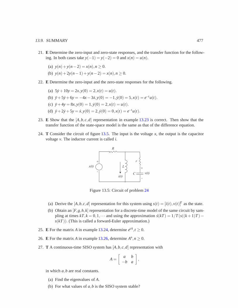
13.9. SUMMARY 477
21. E Determine the zero-input and zero-state responses, and the transfer function for the follow-ing. In both cases take y(−1) = y(−2) = 0 and x(n) = u(n).
(a) y(n)+y(n−2) = x(n),n≥ 0.
(b) y(n)+ 2y(n−1)+y(n−2) = x(n),n≥ 0.
22. E Determine the zero-input and the zero-state responses for the following.
(a) 5y+ 10y = 2x,y(0) = 2,x(t) = u(t).
(b) y+ 5y+ 6y =−4x−3x,y(0) =−1, y(0) = 5,x(t) = e−tu(t).
(c) y+ 4y = 8x,y(0) = 1, y(0) = 2,x(t) = u(t).
(d) y+ 2y+ 5y = x,y(0) = 2, y(0) = 0,x(t) = e−tu(t).
23. E Show that the [A,b,c,d] representation in example 13.23 is correct. Then show that thetransfer function of the state-space model is the same as that of the difference equation.
24. T Consider the circuit of figure 13.5. The input is the voltage x, the output is the capacitorvoltage v. The inductor current is called i.
+
-x(t)
R
L
v(t)i(t)
r
C
+
-
Figure 13.5: Circuit of problem 24
(a) Derive the [A,b,c,d] representation for this system using s(t) = [i(t),v(t)]T as the state.
(b) Obtain an [F,g,h,k] representation for a discrete-time model of the same circuit by sam-pling at times kT,k = 0,1, · · · and using the approximation s(kT) = 1/T(s((k+ 1)T)−s(kT)). (This is called a forward-Euler approximation.)
25. E For the matrix A in example 13.24, determine etA, t ≥ 0.
26. E For the matrix A in example 13.26, determine An,n≥ 0.
27. T A continuous-time SISO system has [A,b,c,d] representation with
A =[
a b−b a
],
in which a,b are real constants.
(a) Find the eigenvalues of A.
(b) For what values of a,b is the SISO system stable?
478 CHAPTER 13. LAPLACE AND Z TRANSFORMS
(c) Calculate etA, t ≥ 0.
(d) Suppose b = c = [1 0]T , and d = 0. Find the transfer function.
28. T Let A be an N×N matrix. Let p be an eigenvalue of A. An N-dimensional (column) vectore, possibly complex-valued, is said to be an eigenvector of A corresponding to p if e �= 0 andAe= pe. Note that an eigenvector always exists since det[pI−A] = 0. Find eigenvectors foreach of the two eigenvalues of the matrices in examples13.24 and 13.26.
29. E Let A be a square matrix with eigenvalue p and corresponding eigenvector e. Determinethe response of the following.
(a) s(k+ 1) = As(k),k≥ 0; s(0) = e.
(b) s(t) = As(t), t ≥ 0; s(0) = e.
Hint. Show that Ane= pne and etAe= epte.
30. T Verify (13.50). Hint. First show that
[sI−A]−1b =1
sN +aN−1sN−1 + · · ·+a0
1s· · ·
sN−1
,
by multiplying both sides by [sI−A]. Then check (13.50).

Chapter 14
Composition and Feedback Control
A major theme of this book is that interesting systems are often compositions of simpler systems.Systems are functions, so their composition is function composition, as discussed in section2.1.5.However, systems are often not directly described as functions, so function composition is not theeasiest tool to use to understand the composition. We have seen systems described as state machines,frequency responses, and transfer functions. In chapter4 we obtained the state machine of the com-posite system from its component state machines. In section8.5 we obtained the frequency responseof the composite system from the frequency response of its component linear time-invariant (LTI)systems. We extend the latter study in this chapter to the composition of LTI systems describedby their transfer functions. This important extension allows us to consider unstable systems whoseimpulse response has a Z or Laplace transform, but not a Fourier transform.
As before, feedback systems prove challenging. A particularly interesting issue is how to maintainstability, and how to construct stable systems out of unstable ones. We will find that some feedbackcompositions of stable systems result in unstable systems, and conversely, some compositions ofunstable systems result in stable systems. For example, we can stabilize the helicopter in example12.2 using feedback, in fact we can precisely control its orientation, despite the intrinsic instability.The family of techniques for doing this is known as feedback control. This chapter serves as anintroduction to that topic. Feedback control can also be used to drive stable systems, in whichcase it serves to improve their response. For example, feedback can result in faster or more preciseresponses, and can also prevent overshoot, where a system overreacts to a command.
We will consider three styles of composition, cascade composition, parallel composition, andfeedback composition. In each case, two LTI systems with transfer functions H1 and H2 are com-bined to get a new system. The transfer functions H1 and H2 are the (Z or Laplace) transforms ofthe respective impulse responses, h1 and h2. Much of our discussion applies equally well whetherthe system is a continuous-time system or a discrete-time system, so in many cases we leave thisunspecified.
479
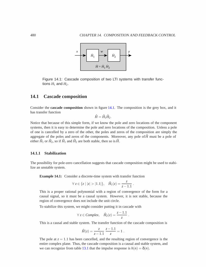
480 CHAPTER 14. COMPOSITION AND FEEDBACK CONTROL
H1
x wH2
y
H = H1 H2
Figure 14.1: Cascade composition of two LTI systems with transfer func-tions H1 and H2.
14.1 Cascade composition
Consider the cascade composition shown in figure 14.1. The composition is the grey box, and ithas transfer function
H = H1H2.
Notice that because of this simple form, if we know the pole and zero locations of the componentsystems, then it is easy to determine the pole and zero locations of the composition. Unless a poleof one is cancelled by a zero of the other, the poles and zeros of the composition are simply theaggregate of the poles and zeros of the components. Moreover, any pole of H must be a pole ofeither H1 or H2, so if H1 and H2 are both stable, then so is H.
14.1.1 Stabilization
The possibility for pole-zero cancellation suggests that cascade composition might be used to stabi-lize an unstable system.
Example 14.1: Consider a discrete-time system with transfer function
∀ z∈ {z | |z|> |1.1|}, H1(z) =z
z−1.1.
This is a proper rational polynomial with a region of convergence of the form for acausal signal, so it must be a causal system. However, it is not stable, because theregion of convergence does not include the unit circle.
To stabilize this system, we might consider putting it in cascade with
∀ z∈Complex, H2(z) =z−1.1
z.
This is a causal and stable system. The transfer function of the cascade composition is
H(z) =z
z−1.1z−1.1
z= 1 .
The pole at z= 1.1 has been cancelled, and the resulting region of convergence is theentire complex plane. Thus, the cascade composition is a causal and stable system, andwe can recognize from table 13.1 that the impulse response is h(n) = δ(n).

14.1. CASCADE COMPOSITION 481
Stabilizing systems by cancelling their poles in a cascade composition, however, is almost never agood idea. If the pole is not precisely cancelled, then no matter how small the error, the resultingsystem is still unstable.
Example 14.2: Suppose that in the previous example the pole location is not knownprecisely, and turns out to be at z= 1.1001 instead of z= 1.1. Then the cascade com-position has transfer function
H(z) =z
z−1.1001z−1.1
z=
z−1.1z−1.1001
,
which is unstable.
14.1.2 Equalization
While cascade compositions do not usually work well for stabilization, they do often work well forequalization. An equalizer is a compensator that reverses distortion. The source of the distortion,which is often called a channel, must be an LTI system, and the equalizer is composed in cascadewith it. At first sight this is easy to do. If the channel has transfer function H1, then the equalizercould have transfer function
H2 = H−11 ,
in which case the cascade composition will have transfer function
H = H1H2 = 1,
which is certainly distortion-free.
Example 14.3: Some acoustic environments for audio have resonances, where certainfrequencies are enhanced as the sound propagates through the environment (see labC.8for an example). This will typically occur if the physics of the acoustic environmentresults in a transfer function with poles near the unit circle (for a discrete-time model)or near the imaginary axis (for a continuous-time model). Suppose for example thatthe acoustic environment is well modeled by a discrete-time LTI system with transferfunction
∀ z∈ {z | |z|> 0.95}, H1(z) =z2
(z−a)(z−a∗),
where a = 0.95eiω1 for some frequency ω1. Using the methods of section 13.2, we caninfer that the magnitude response will have a strong peak at frequencies ω1 and −ω1,because the positions on the unit circle eiω1 and e−iω1 are very close to the poles. Thiswill result in distortion of the audio signal, where frequencies near ω1 will be amplified.
An equalizer that will compensate for this distortion has transfer function
H2(z) = [H1(z)]−1 =(z−a)(z−a∗)
z2 =z2−2Re{a}z+ |a|2
z2 .
482 CHAPTER 14. COMPOSITION AND FEEDBACK CONTROL
As in example 13.2, we can recognize this as the Z transform of an FIR filter withimpulse response
∀ n∈ Integers, h2(n) = δ(n)−2Re{a}δ(n−1)+ |a|2δ(n−2).
This filter is causal and stable, and hence can serve as an effective equalizer.
There are a number of potential problems with this approach, however. First, the transfer functionof the channel is probably not known, or at least not known precisely. Second, the channel may nothave a stable and causal inverse.
Let us first examine the first difficulty, that the channel may not be known (precisely). If the channelmodel H1 and its inverse H2 are both stable, then the cascade composition is at least assured of beingstable, even if the channel has been misconstrued. Moreover, if the equalizer is close to the inverseof the true channel, then often the distortion is significantly reduced despite the errors (see exercise1).
This difficulty can sometimes be dealt with by adaptively varying the equalizer based on measure-ments of the distortion. One way to measure the distortion is to send through the channel a knownsequence called a training sequence and observe the output of the channel. Suppose that the train-ing sequence is a signal x with Z transform X, and that the channel H1 is unknown. If we can observethe output y of the channel, and calculate its Z transform Y, then the channel transfer function issimply
∀ z∈RoC(h1), H1(z) =Y(z)X(z)
,
where RoC(h1) is determined by identifying the poles and zeros of the rational polynomialY(z)/X(z)and finding the one ring-shaped region that includes the unit circle and is bordered by poles. Thisresults in a stable channel model.
Training sequences are commonly used in digital communication systems, where, for example, aradio channel introduces distortion. However, it is also common for such channels to change overtime. Radio channels, for example, change if either the transmitter or receiver moves, or if theweather changes, or if obstacles appear or disappear. Repeatedly transmitting training sequences isan expensive waste of radio bandwidth, and fortunately, is not usually necessary, as illustrated in thefollowing example.
Example 14.4: Consider a digital communication system where the channel is mod-eled as a discrete-time LTI system with transfer function H1, representing for examplea radio transmission subsystem. Suppose that this digital communication system trans-mits a bit sequence represented as a discrete-time signal x of form
x: Integers→{0,1}.Suppose further that we use a training sequence to obtain an initial estimate H2 ofthe inverse of the channel. But over time, the channel drifts, so that H2 is no longerthe inverse of H1. Assuming the drift is relatively slow, then after a short time, H2 isstill close to the inverse of H1, in that the cascade H1H2 yields only mild distortion.
14.1. CASCADE COMPOSITION 483
That is, if x(n) = 0 for some n, then y(n) ≈ 0. Similarly, if x(n) = 1 for some n, theny(n) ≈ 1. Thus, we can quantize y, getting an accurate estimate x without it having tobe a known training sequence. That is, when y(n) ≈ 0, we assume that x(n) = 0, andwhen y(n) ≈ 1, we assume that x(n) = 1. These assumptions are called decisions, andin fact, such decisions must be made anyway for digital communication to occur. Wehave to decide whether a 1 or a 0 was transmitted, and closeness to 1 or 0 seems like aneminently reasonable basis on which to make such a decision.
Assuming there are no errors in these decisions, we can infer that
H1H2Xd = Y,
where Xd is the Z transform of the decision sequence. So, without using another trainingsequence, we can revise our estimate of the channel transfer function as follows,
H1 =Y
H2Xd.
We replace our equalizer H2 with
H ′2 = [H1]−1 =H2Xd
Y.
Of course, we now start using H ′2, which will come closer to correcting the channeldistortion, which will make our decisions more reliable for the next update.
Example 14.4 outlines a widely used technique called decision-directed adaptive equalization.It is so widely used, in fact, that it may be found in every digital cellular telephone and almostevery modem, including voiceband data modems, radio modems, cable modems, DSL modems,etc. The algorithms used in practice to update the transfer function of the equalizer are not exactlyas shown in the example, and their details are beyond the scope of this text, but they follow thegeneral principle in the example.
Let us now turn our attention to the second difficulty with equalization, that the channel may nothave a stable and causal inverse. We begin with an example.
Example 14.5: Suppose that, similar to example 14.3, a channel has transfer function
∀ z in{z | |z|> 0.95}, H1(z) =z
(z−a)(z−a∗),
where a = 0.95eiω1 for some frequency ω1. The inverse is
[H1(z)]−1 =(z−a)(z−a∗)
z=
z2−2Re{a}z+ |a|2)z
,
which is not a proper rational polynomial. Thus, this cannot be the Z transform of acausal signal. Implementing a non-causal equalizer will usually be impossible, sinceit will require knowing future inputs. However, suppose we simply force the equalizer

484 CHAPTER 14. COMPOSITION AND FEEDBACK CONTROL
have a proper rational polynomial transfer function by dividing by a high enough powerM of z to make [H1(z)]−1/zM proper. In this example, M = 1 is sufficient, so we definethe equalizer to be
H2(z) =[H1(z)]−1
z=
z2−2Re{a}z+ |a|2)z2 ,
which we again recognize as the Z transform of an FIR filter with impulse response
∀ n∈ Integers, h2(n) = δ(n)−2Re{a}δ(n−1)+ |a|2δ(n−2).
This filter is causal and stable, but does it serve as an effective equalizer? Consider nowthe cascade,
H(z) = H1(z)H2(z) =1z.
From section 13.1.2 we recognize this as the transfer function of the unit delay system.That is, the equalizer completely compensates for the distortion, but at the expense ofintroducing a one sample delay. This is usually a perfectly acceptable cost.
Example 14.5 demonstrates that when the channel inverse is not a proper rational polynomial, thenintroducing a delay may enable construction of a stable and causal equalizer. Not all equalizationstories have such a happy ending, however. Consider the following example.
Example 14.6: Consider a channel with the following transfer function,
∀ z∈ {z∈ Complex| z �= 0}, H1(z) =z−2
z.
This is a stable and causal channel. Its inverse is
[H1(z)]−1 =z
z−2.
This has a pole at z = 2, so in order to be stable, it would have to be anti-causal (sothat the region of convergence can include the unit circle). Implementing an anti-causalequalizer is usually not possible.
Example 14.6 shows that not all channels can be inverted by an equalizer. All is not lost, however.Given a channel H1(z) that has a rational Z transform, we can usually find a transfer functionH2(z)that compensates for the magnitude response part of the distortion. That is, we can find a transferfunction H2(z) that is stable and causal such that the magnitude response of the composite satisfies
|H1(ω)H2(ω)| = |H1(eiω)H2(eiω)|= 1.
For some applications, this is sufficient. In audio equalization, for example, this is almost alwayssufficient, because the human ear is not very sensitive to the phase of audio signals. It hears onlythe magnitude of the frequency components.
14.2. PARALLEL COMPOSITION 485
Example 14.7: Continuing example 14.6, let H2 be given by
H2 =z
1−2z=−0.5zz−0.5
.
This has a pole at z= 0.5, and is a proper rational polynomial, so it can be the transferfunction of a causal and stable filter. Consider the cascade composition,
H(z) = H1(z)H2(z) =z−2
z· −0.5zz−0.5
=1−0.5zz−0.5
.
This hardly looks like what we want, but if we rewrite it slightly, it is easy to show thatthe magnitude frequency response has value one for all ω,
H(z) =1−0.5zz−0.5
= zz−1−0.5z−0.5
.
The magnitude frequency response is
|H(ω)|= |H(eiω)|= |eiω| · |e−iω−0.5||eiω−0.5| = 1 .
This magnitude is equal to 1 because the numerator, e−iω−0.5, is the complex conju-gate of the denominator, eiω−0.5, so they have the same magnitude.
The method in example 14.7 can be generalized so that for most channels it is possible to cancelany magnitude distortion. The key is that if the channel transfer function has a zero outside the unitcircle, say at z= a, then its inverse has a pole at the same location, z= a. A pole outside the unitcircle makes it impossible to have a stable and causal filter. So the trick is to place a pole instead atz= 1/a∗. This pole will cancel the effect on the magnitude (but not the phase) of the zero at z= a.
There are still channels for which this method will not work.
Example 14.8: Consider a channel given by
∀ z∈ {z∈ Complex| z �= 0}, H1(z) =z−1
z.
This has a pole at z = 0 and a zero at z = 1. Its inverse cannot be stable because itwill have a pole at z= 1. In fact, no equalization is possible. This is intuitive becausethe frequency response is zero at ω = 0, and no stable equalizer in cascade with thischannel can reconstruct the original component at ω= 0. It would have to have infinitegain at ω= 0, which would make it unstable.
14.2 Parallel composition
Consider the parallel composition shown in figure 14.2. The transfer function of the compositionsystem is
H = H1 + H2.
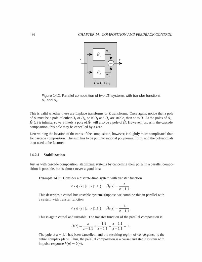
486 CHAPTER 14. COMPOSITION AND FEEDBACK CONTROL
H1
x
w1
H2
y
H = H1+ H2
w2
Figure 14.2: Parallel composition of two LTI systems with transfer functionsH1 and H2.
This is valid whether these are Laplace transforms or Z transforms. Once again, notice that a poleof H must be a pole of either H1 or H2, so if H1 and H2 are stable, then so is H. At the poles of H1,H1(z) is infinite, so very likely a pole of H1 will also be a pole of H. However, just as in the cascadecomposition, this pole may be cancelled by a zero.
Determining the location of the zeros of the composition, however, is slightly more complicated thanfor cascade composition. The sum has to be put into rational polynomial form, and the polynomialsthen need to be factored.
14.2.1 Stabilization
Just as with cascade composition, stabilizing systems by cancelling their poles in a parallel compo-sition is possible, but is almost never a good idea.
Example 14.9: Consider a discrete-time system with transfer function
∀ z∈ {z | |z|> |1.1|}, H1(z) =z
z−1.1.
This describes a causal but unstable system. Suppose we combine this in parallel witha system with transfer function
∀ z∈ {z | |z|> |1.1|}, H2(z) =−1.1
z−1.1.
This is again causal and unstable. The transfer function of the parallel composition is
H(z) =z
z−1.1+−1.1
z−1.1=
z−1.1z−1.1
= 1 .
The pole at z= 1.1 has been cancelled, and the resulting region of convergence is theentire complex plane. Thus, the parallel composition is a causal and stable system withimpulse response h(n) = δ(n).
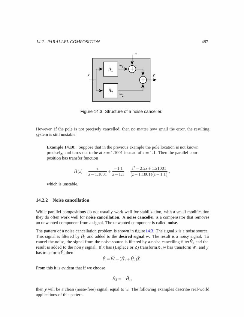
14.2. PARALLEL COMPOSITION 487
H1
x
w
H2
y
w1
w2
Figure 14.3: Structure of a noise canceller.
However, if the pole is not precisely cancelled, then no matter how small the error, the resultingsystem is still unstable.
Example 14.10: Suppose that in the previous example the pole location is not knownprecisely, and turns out to be at z= 1.1001 instead of z= 1.1. Then the parallel com-position has transfer function
H(z) =z
z−1.1001+−1.1
z−1.1=
z2−2.2z+ 1.21001(z−1.1001)(z−1.1)
,
which is unstable.
14.2.2 Noise cancellation
While parallel compositions do not usually work well for stabilization, with a small modificationthey do often work well for noise cancellation. A noise canceller is a compensator that removesan unwanted component from a signal. The unwanted component is called noise.
The pattern of a noise cancellation problem is shown in figure14.3. The signal x is a noise source.This signal is filtered by H1 and added to the desired signal w. The result is a noisy signal. Tocancel the noise, the signal from the noise source is filtered by a noise cancelling filterH2 and theresult is added to the noisy signal. If x has (Laplace or Z) transform X, w has transform W, and yhas transform Y, then
Y = W +(H1 + H2)X.
From this it is evident that if we choose
H2 =−H1,
then y will be a clean (noise-free) signal, equal to w. The following examples describe real-worldapplications of this pattern.
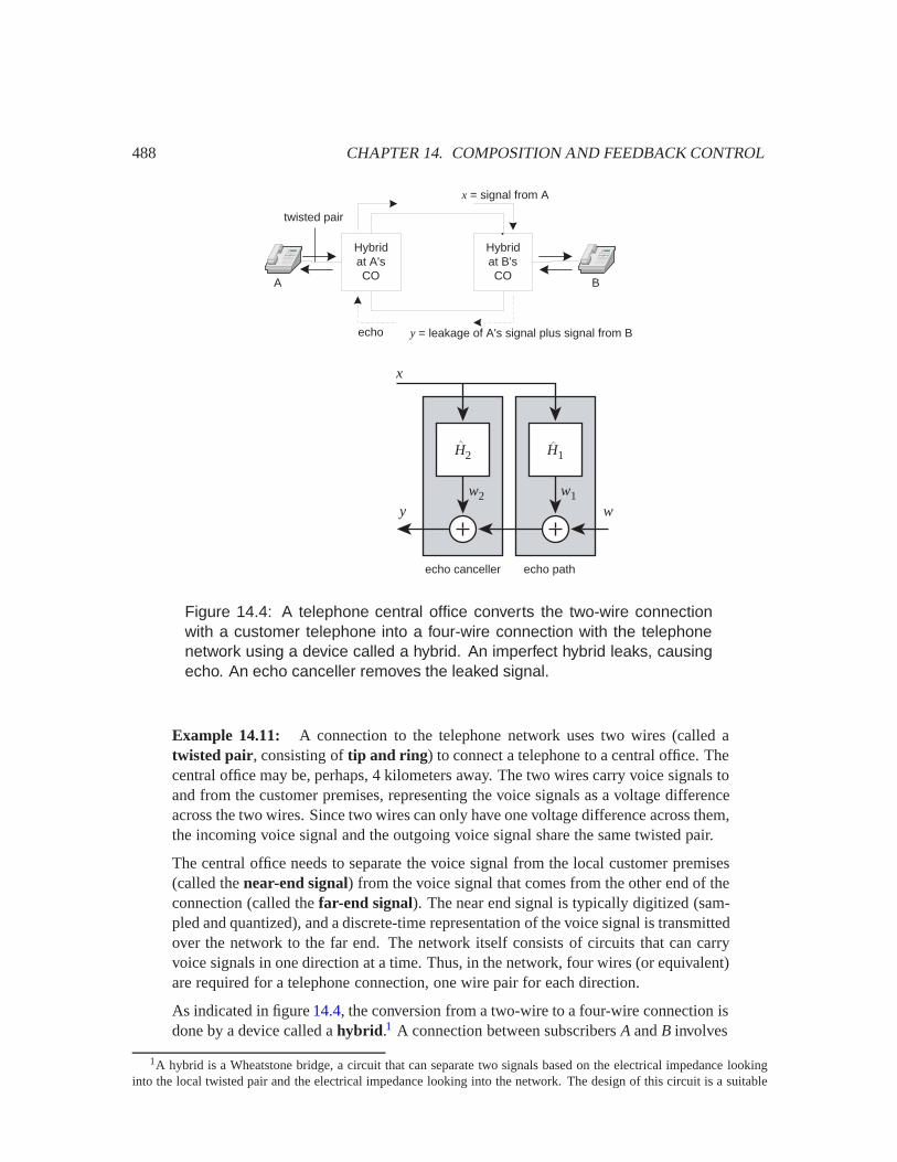
488 CHAPTER 14. COMPOSITION AND FEEDBACK CONTROL
A B
Hybridat A'sCO
Hybridat B'sCO
x = signal from A
y = leakage of A's signal plus signal from Becho
twisted pair
H1
x
w
H2
y
echo pathecho canceller
w1w2
Figure 14.4: A telephone central office converts the two-wire connectionwith a customer telephone into a four-wire connection with the telephonenetwork using a device called a hybrid. An imperfect hybrid leaks, causingecho. An echo canceller removes the leaked signal.
Example 14.11: A connection to the telephone network uses two wires (called atwisted pair, consisting of tip and ring) to connect a telephone to a central office. Thecentral office may be, perhaps, 4 kilometers away. The two wires carry voice signals toand from the customer premises, representing the voice signals as a voltage differenceacross the two wires. Since two wires can only have one voltage difference across them,the incoming voice signal and the outgoing voice signal share the same twisted pair.
The central office needs to separate the voice signal from the local customer premises(called the near-end signal) from the voice signal that comes from the other end of theconnection (called the far-end signal). The near end signal is typically digitized (sam-pled and quantized), and a discrete-time representation of the voice signal is transmittedover the network to the far end. The network itself consists of circuits that can carryvoice signals in one direction at a time. Thus, in the network, four wires (or equivalent)are required for a telephone connection, one wire pair for each direction.
As indicated in figure 14.4, the conversion from a two-wire to a four-wire connection isdone by a device called a hybrid.1 A connection between subscribers A and B involves
1A hybrid is a Wheatstone bridge, a circuit that can separate two signals based on the electrical impedance lookinginto the local twisted pair and the electrical impedance looking into the network. The design of this circuit is a suitable
14.2. PARALLEL COMPOSITION 489
two hybrids, one in each subscriber’s central office. The hybrid in B’s central officeideally will pass all of the incoming signal x to B’s two-wire circuit, and none back intothe network. However, the hybrid is not perfect, and some of the incoming signal xleaks through the hybrid into the return path back to A. The signal y in the figure is thesum of the signal from B and the leaked signal from A. A hears the leaked signal as anecho, since it is A’s own signal, delayed by propagation through the telephone network.
If the telephone connection includes a satellite link, then the delay from one end of theconnection to the other is about 300ms. This is the time it takes for a radio signal topropagate to a geosynchronous satellite and back. The echo traverses this link twice:once going from A to B, and the second time coming back. Thus, the echo is A’sown signal delayed by about 600ms. For voice signals, 600ms of delay is enough tocreate a very annoying echo that can make it difficult to speak. Humans have difficultyspeaking when they hear their own voices 600ms later. Consequently, the designers ofthe telephone network have put echo cancellers in to prevent the echo from occuring.
Let H1 be the transfer function of the hybrid leakage path. The echo canceller is thefilter H2 placed in parallel composition with the hybrid, as shown in the figure. Theoutput w2 of this filter is added to the output w1 + w of the hybrid, so the signal thatactually goes back is y = w2 +w1 +w. If
H2 =−H1,
then y = w and the echo is cancelled perfectly. Moreover, note that as long as H1 isstable and causal, so will be the echo canceller H2.
However, H1 is not usually known in advance, and also it changes over time. So eithera fixed H2 is designed to match a ‘typical’ H1, or an adaptive echo canceller is designedthat estimates the characteristics of the echo path (H1) and changes H2 accordingly.Adaptive echo cancellers are common in the telephone network today.
The following example combines cascade and parallel composition to achieve noise cancellation.
Example 14.12: Consider a microphone in a noisy environment. For example, atraffic helicopter might be used to deliver live traffic reports over the radio, but the(considerable) background noise of the helicopter would be highly undesirable on theradio. Fortunately, the background noise can be cancelled. Referring to figure14.5,suppose that w is the announcer’s voice, x is the engine noise, and H1 represents theacoustic path from the engine noise to the microphone. The microphone picks up boththe engine noise and the announcer’s voice, producing the noisy signal w4. We canplace a second microphone somewhere far enough from the announcer so as to not pickup much of his or her voice. Since this microphone is in a different place, say on theback of the announcer’s helmet, the acoustic path is different, so we model that pathwith another transfer function H2. To cancel the noise, we design a filter H3. This filterneeds to equalize (invert) H2 and cancel H1. That is, its ideal value is
H3 =−H1/H2.
topic for a text on electrical circuits.
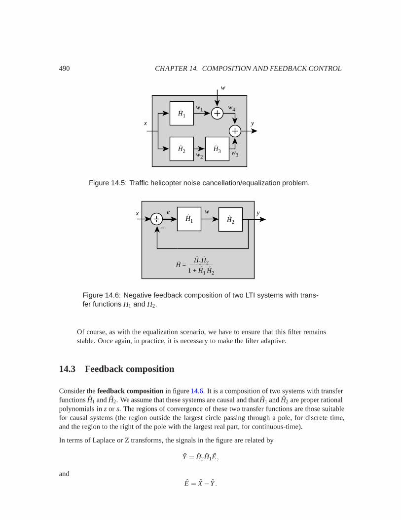
490 CHAPTER 14. COMPOSITION AND FEEDBACK CONTROL
H1
x
w
H2
y
w1
w2
H3 w3
w4
Figure 14.5: Traffic helicopter noise cancellation/equalization problem.
H1
x eH2
y
H =
w
H1H2
1 + H1 H2
−
Figure 14.6: Negative feedback composition of two LTI systems with trans-fer functions H1 and H2.
Of course, as with the equalization scenario, we have to ensure that this filter remainsstable. Once again, in practice, it is necessary to make the filter adaptive.
14.3 Feedback composition
Consider the feedback composition in figure 14.6. It is a composition of two systems with transferfunctions H1 and H2. We assume that these systems are causal and thatH1 and H2 are proper rationalpolynomials in z or s. The regions of convergence of these two transfer functions are those suitablefor causal systems (the region outside the largest circle passing through a pole, for discrete time,and the region to the right of the pole with the largest real part, for continuous-time).
In terms of Laplace or Z transforms, the signals in the figure are related by
Y = H2H1E,
andE = X−Y.

14.3. FEEDBACK COMPOSITION 491
Notice that, by convention, the feedback term is subtracted, as indicated by the minus sign adjacentto the adder (for this reason, this composition is called negative feedback). Combining these twoequations to elimintate E, we get
Y = H1H2(X−Y),
which we can solve for the transfer function of the composition,
H =Y
X=
H1H2
1+ H1H2. (14.1)
This is often called the closed-loop transfer function, to contrast it with the open-loop transferfunction, which is simply H1H2. We will assume that this resulting system is causal, and that the re-gion of convergence of this transfer function is therefore determined by the roots of the denominatorpolynomial, 1+ H1H2.
The closed-loop transfer function is valid as long as the denominator 1 +H1H2 is not identicallyzero (that is, it is not zero for all s or z in Complex– it may be zero some sor z in Complex). Thisis sufficient for the feedback loop to be well-formed, although in general, this fact is not trivial todemonstrate (exercise 8 considers the easier case where H1H2 is causal and strictly proper, in whichcase the system H1H2 has state-determined output). We will assume henceforth, without comment,that the denominator is not identically zero.
Feedback composition is useful for stabilizing unstable systems. In the case of cascade and parallelcomposition, a pole of the composite must be a pole of one of the components. The only way toremove or alter a pole of the components is to cancel it with a zero. For this reason, cascade and par-allel composition are not effective for stabilizing unstable systems. Any error in the specification ofthe unstable pole location results in a failed cancellation, which results in an unstable composition.
In contrast, the poles of the feedback composition are the roots of the denominator 1+H1H2, whichare generally quite different from the poles of H1 and H2. This leads to the following importantconclusion:
The poles of a feedback composition can be different from the poles of its com-ponent subsystems. Consequently, unstable system can be effectively and robustlystabilized by feedback.
The stabilization is robust in that small changes in the pole or zero locations do not result in thecomposition going unstable. We will be able to quantify this robustness.
14.3.1 Proportional controllers
In control applications, one of the two systems being composed, sayH2, is called the plant. This is aphysical system that is given to us to control. Its transfer function is determined by its physics. Thesecond system being composed, say H1, is the controller. We design this system to get the plantto do what we want. The following example illustrates a simple strategy called a proportionalcontroller or P controller.

492 CHAPTER 14. COMPOSITION AND FEEDBACK CONTROL
H1=Kx e
H2
y
H =
w
K / M
s + K / M
−Ms1=
desiredangularvelocity
angularvelocity
torqueerror
Figure 14.7: A negative feedback proportional controller with gain K.
Example 14.13: For this example we take as the plant the simplified continuous-timehelicopter model of example 12.2,
y(t) =1M
w(t).
Here y(t) is the angular velocity at time t and w(t) is the torque. M is the moment ofinertia.
We have renamed the input w (instead of x) because we wish to control the helicopter,and the control input signal will not be the torque. Instead, let’s define the input x tobe the desired angular velocity. So, to get the helicopter to not rotate, we provide inputx(t) = 0.
Let us call the impulse response of the plant h2, to conform with the notation in figure14.6; it is given by
∀ t ∈ Reals, h2(t) = u(t)/M,
where u is the unit step. The transfer function is H2(s) = 1/(Ms), with RoC(h) = {s∈Complex| Re(s) > 0}. H2 has a pole at s= 0, so this is an unstable system.
As a compensator we can simply place a gain K in a negative feedback composition,as shown in figure 14.7. The intuition is as follows. Suppose we wish to keep the he-licopter from rotating. That is, we would like the output angular velocity to be zero,y(t) = 0. Then we should apply an input of zero, x(t) = 0. However, the plant is un-stable, so even with a zero input, the output diverges (even the smallest non-zero initialcondition or the smallest input disturbance will cause it to diverge). With the feedbackarrangement in figure 14.7, if the output angular velocity rises above zero, then the in-put is modified downwards (the feedback is negative), which will result in a negativetorque being applied to the plant, which will counter the rising velocity. If the outputangular velocity drops below zero, then the torque will be modified upwards, whichagain will tend to counter the dropping velocity. The output velocity will stabilize atzero.
To get the helicopter to rotate, for example to execute a turn, we simply apply a non-zero input. The feedback system will again compensate so that the helicopter will rotateat the angular velocity specified by the input.

14.3. FEEDBACK COMPOSITION 493
2− −2
K = −2K = +2 K = −K =
root locus
K = 0
Figure 14.8: Root locus of the helicopter P controller.
The signal e is the difference between the input x, which is the desired angular velocity,and the output y, which is the actual angular velocity. It is called the error signal.Intuitively, this signal is zero when everything is as desired, when the output angularvelocity matches the input.
A compensator like that in example 14.13 and figure 14.7 is called a proportional controller orP controller. The input w to the plant is proportional to the error e. The objective of the controlsystem is to have the output y of the plant track the input x as closely as possible. I.e., the error eneeds to be small. We can use (14.1) to find the transfer function of the closed-loop system.
Example 14.14: Continuing with the helicopter of example 14.13, the closed loopsystem transfer function is
G(s) =KH(s)
1+KH(s)=
K/Ms+K/M
. (14.2)
which has a pole at s=−K/M. If K > 0, the closed loop system is stable, and if K < 0,it is unstable. Thus, we have considerable freedom to choose K. How should we chooseits value?
As K increases from 0 to ∞, the pole at at s = −K/M moves left from 0 to −∞. AsK decreases from 0 to −∞, the pole moves to the right from 0 to ∞. The locus of thepole as K varies is called the root locus, since the pole is a root of the denominatorpolynomial.
Figure 14.8 shows the root locus as a thick gray line, on which are marked the locationsof the pole for K = 0,±2,±∞. Since there is only one pole, the root locus comprisesonly one ‘branch’. In general the root locus has as many branches as the number ofpoles, with each branch showing by the movement of one pole as K varies.
Note that in principle, the same transfer function as the closed-loop transfer function can be achievedby a cascade composition. But as in example14.1, the resulting system is not robust, in that even thesmallest change in the pole location of the plant can cause the system to go unstable (see problem6). The feedback system, however, is robust, as shown in the following example
494 CHAPTER 14. COMPOSITION AND FEEDBACK CONTROL
Example 14.15: Continuing with the P controller for the helicopter, suppose that ourmodel of the plant is not perfect, and its actual transfer function is
H2(s) =1
M(s− ε),
for some small value of ε > 0. In that case, the closed loop transfer function is
H(s) =K/M
s− ε+K/M,
which has a pole at s= ε−K/M. So the feedback system remains stable so long as
ε < K/M.
In practice, when designing feedback controllers, we first quantify our uncertainty about the plant,and then determine the controller parameters so that under all possible plant transfer functions, theclosed-loop system is stable.
Example 14.16: Continuing the helicopter example, we might say that ε < 0.5. In thatcase, if we choose K so that K/M > 0.5, we would guarantee stability for all values ofε < 0.5. We then say that the proportional feedback controller is robust for all plantswith ε < 0.5.
We still have a large number of choices for K. How do we select one? To understand the implicationsof different choices of K we need to study the behavior of the output y (or the error signal e) fordifferent choices of K. In the following examples we use the closed-loop transfer function to analyzethe response of a proportional controller system to various inputs. The first example studies theresponse to a step function input.
Example 14.17: Continuing the helicopter example, suppose that the input is a stepfunction, ∀t,x(t) = au(t) where a is a constant and u is the unit step. This input declaresthat at time t = 0, we wish for the helicopter to begin rotating with angular velocity a.The closed-loop transfer function is given by (14.2), and the Laplace transform of x isX(s) = a/s, from table 13.3, so the Laplace transform of the output is
Y(s) = G(s)X(s) =K/M
s+K/M· a
s
Carrying out the partial fraction expansion, this becomes
Y(s) =−a
s+K/M+
as
.
We can use this to find the inverse Laplace transform,
∀t, y(t) =−ae−Kt/Mu(t)+au(t).
The second term is the steady-state response yss, which in this case equals the input.So the first term is the tracking error ytr , which goes to zero faster for larger K. Hencefor step inputs, the larger the gain K, the smaller the tracking error.
14.3. FEEDBACK COMPOSITION 495
In the previous example, we find that the error goes to zero when the input is a step function.Moreover, the error goes to zero faster if the gain K is larger than if it is smaller. In the followingexample, we find that if the input is sinusoidal, then larger gain K results in an ability to track higherfrequency inputs.
Example 14.18: Suppose the input to the P controller helicopter system is a sinusoidof amplitude A and frequency ω0,
∀ t ∈ Reals, x(t) = A(cosω0t)u(t).
We know that the response can be decomposed as y = ytr +yss. The transient responseytr is due to the pole at s=−K/M, and so it is of the form
∀ t ∈ Reals, ytr(t) = Re−Kt/M,
for some constant R. The steady-state response is determined by the frequency responseat ω0. The frequency response is
∀ ω∈ Reals, H(ω) = H(iω) =K/M
iω+K/M,
with magnitude and phase given by
|H(ω)|= K/M
[ω2 +(K/M)2]1/2, � H(ω) =− tan−1 ωM
K.
So the steady-state response is
∀t, yss(t) = |H(ω0)|Acos(ω0t + � H(ω0)).
Thus the steady-state output is a sinusoid of the same frequency as the input but with asmaller amplitude (unless ω0 = 0). The larger ω0 is, the smaller the output amplitude.Hence, the ability of the closed-loop system to track a sinusoidal input decreases as thefrequency of the sinusoidal input increases. However, increasing K reduces this effect.Thus, larger gain in the feedback loop improves its ability to track higher frequencysinusoidal inputs.
In addition to the reduction in amplitude, the output has a phase difference. Again,if ω0 = 0, there is no phase error, because tan−1(0) = 0. As ω0 increases, the phaselag increases (the phase angle decreases). Once again, however, increasing the gain Kreduces the effect.
The previous two examples suggest that large gain in the feedback loop is always better. For a stepfunction input, it causes the transient error to die out faster. For a sinusoidal input, it improves theability to track higher frequency inputs, and it reduces the phase error in the tracking. A large gainis not always a good idea, however, as seen in the next example, a DC motor.

496 CHAPTER 14. COMPOSITION AND FEEDBACK CONTROL
Example 14.19: The angular position y of a DC motor is determined by the inputvoltage w according to the differential equation
My(t)+Dy(t) = Lw(t),
where M is the moment of inertia of the rotor and attached load, Dy is the dampingforce, and the torqe Lw is proportional to the voltage. The transfer function is
H2(s) =L
Ms2 +Ds=
L/Ms(s+D/M)
.
which has one pole at s = 0 and one pole at s = −D/M. By itself the DC motor isunstable because of the pole at s= 0. The transfer function of the feedback compositionwith proportional gain K is
H(s) =KH2(s)
1+KH2(s)=
KLMs2 +Ds+KL
.
There are two closed loop poles—the roots of Ms2 +Ds+KL—located at
s=− D2M±
√D2
4M2 −KLM
.
The closed loop system is stable if both poles have negative real parts, which is the caseif K > 0. If K < D2/(4ML) both poles are real. But if K > D2/(4ML), the two polesform a complex conjugate pair located at
s=− D2M± i
√KLM− D2
4M2 .
The real part is fixed at D/2M, but the imaginary part increases with K. We investigateperformance for the parameter values L/M = 10,D/M = 0.1. The transfer function is
H(s) =10K
s2 + 0.1s+ 10K.
Because there are two poles, the root locus has two branches, as shown in figure14.9.For K = 0, the two poles are located at 0 and -0.1, as illustrated by crosses in thefigure. As K increases the two poles move towards each other, coinciding at -0.05when K = 0.00025. For larger values of K, the two branches split into a pair of complexconjugate poles.
To appreciate what values of K > 0 to select for good tracking, we consider the responseto a step input x = u(t) for two different values of K. For K = 0.00025, the Laplacetransform of the output y is
Y(s) =10K
s2 + 0.1s+ 10K1s
=0.0025
(s+ 0.05)2
1s
=− 1s+ 0.05
− 0.05(s+ 0.05)2 +
1s
.
So the time domain response is
∀t, y(t) = {−e−0.05t −0.05te−0.05t}u(t)+u(t). (14.3)
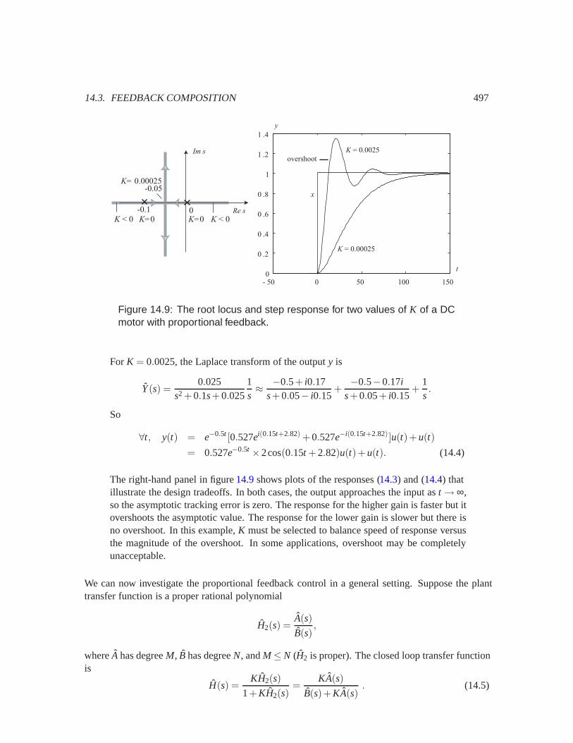
14.3. FEEDBACK COMPOSITION 497
-0.05
-0.1 0K=0
K= 0.00025
K < 0Re s
Im s
K=0K < 0
- 50 0 50 100 1500
0 .2
0 .4
0 .6
0 .8
1
1 .2
1 .4
K = 0.0025
K = 0.00025
t
y
x
overshoot
Figure 14.9: The root locus and step response for two values of K of a DCmotor with proportional feedback.
For K = 0.0025, the Laplace transform of the output y is
Y(s) =0.025
s2 + 0.1s+ 0.0251s≈ −0.5+ i0.17
s+ 0.05− i0.15+−0.5−0.17i
s+ 0.05+ i0.15+
1s.
So
∀t, y(t) = e−0.5t [0.527ei(0.15t+2.82) + 0.527e−i(0.15t+2.82)]u(t)+u(t)= 0.527e−0.5t ×2cos(0.15t + 2.82)u(t)+u(t). (14.4)
The right-hand panel in figure 14.9 shows plots of the responses (14.3) and (14.4) thatillustrate the design tradeoffs. In both cases, the output approaches the input as t→ ∞,so the asymptotic tracking error is zero. The response for the higher gain is faster but itovershoots the asymptotic value. The response for the lower gain is slower but there isno overshoot. In this example, K must be selected to balance speed of response versusthe magnitude of the overshoot. In some applications, overshoot may be completelyunacceptable.
We can now investigate the proportional feedback control in a general setting. Suppose the planttransfer function is a proper rational polynomial
H2(s) =A(s)B(s)
,
where A has degree M, B has degree N, and M≤N (H2 is proper). The closed loop transfer functionis
H(s) =KH2(s)
1+KH2(s)=
KA(s)B(s)+KA(s)
. (14.5)
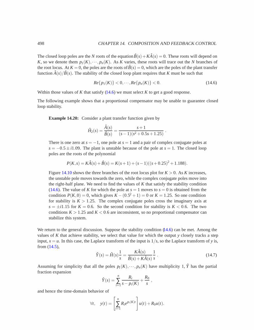
498 CHAPTER 14. COMPOSITION AND FEEDBACK CONTROL
The closed loop poles are the N roots of the equation B(s)+KA(s) = 0. These roots will depend onK, so we denote them p1(K), · · · , pn(K). As K varies, these roots will trace out the N branches ofthe root locus. At K = 0, the poles are the roots of B(s) = 0, which are the poles of the plant transferfunction A(s)/B(s). The stability of the closed loop plant requires that K must be such that
Re{p1(K)}< 0, · · · ,Re{pn(K)}< 0. (14.6)
Within those values of K that satisfy (14.6) we must select K to get a good response.
The following example shows that a proportional compensator may be unable to guarantee closedloop stability.
Example 14.20: Consider a plant transfer function given by
H2(s) =A(s)B(s)
=s+ 1
(s−1)(s2 + 0.5s+ 1.25).
There is one zero at s=−1, one pole at s= 1 and a pair of complex conjugate poles ats= −0.5± i1.09. The plant is unstable because of the pole at s= 1. The closed looppoles are the roots of the polynomial
P(K,s) = KA(s)+ B(s) = K(s+ 1)+ (s−1)((s+ 0.25)2 + 1.188).
Figure 14.10 shows the three branches of the root locus plot for K > 0. As K increases,the unstable pole moves towards the zero, while the complex conjugate poles move intothe right-half plane. We need to find the values of K that satisfy the stability condition(14.6). The value of K for which the pole at s= 1 moves to s= 0 is obtained from thecondition P(K,0) = 0, which gives K− (0.52 + 1) = 0 or K = 1.25. So one conditionfor stability is K > 1.25. The complex conjugate poles cross the imaginary axis ats = ±i1.15 for K = 0.6. So the second condition for stability is K < 0.6. The twoconditions K > 1.25 and K < 0.6 are inconsistent, so no proportional compensator canstabilize this system.
We return to the general discussion. Suppose the stability condition (14.6) can be met. Among thevalues of K that achieve stability, we select that value for which the output y closely tracks a stepinput, x = u. In this case, the Laplace transform of the input is 1/s, so the Laplace transform of y is,from (14.5),
Y(s) = H(s)1s
=KA(s)
B(s)+KA(s)1s
. (14.7)
Assuming for simplicity that all the poles p1(K), · · · , pn(K) have multiplicity 1, Y has the partialfraction expansion
Y(s) =n
∑i=1
Ri
s− pi(K)+
R0
s,
and hence the time-domain behavior of
∀t, y(t) =
[n
∑i=1
Riepi (K)t
]u(t)+R0u(t).
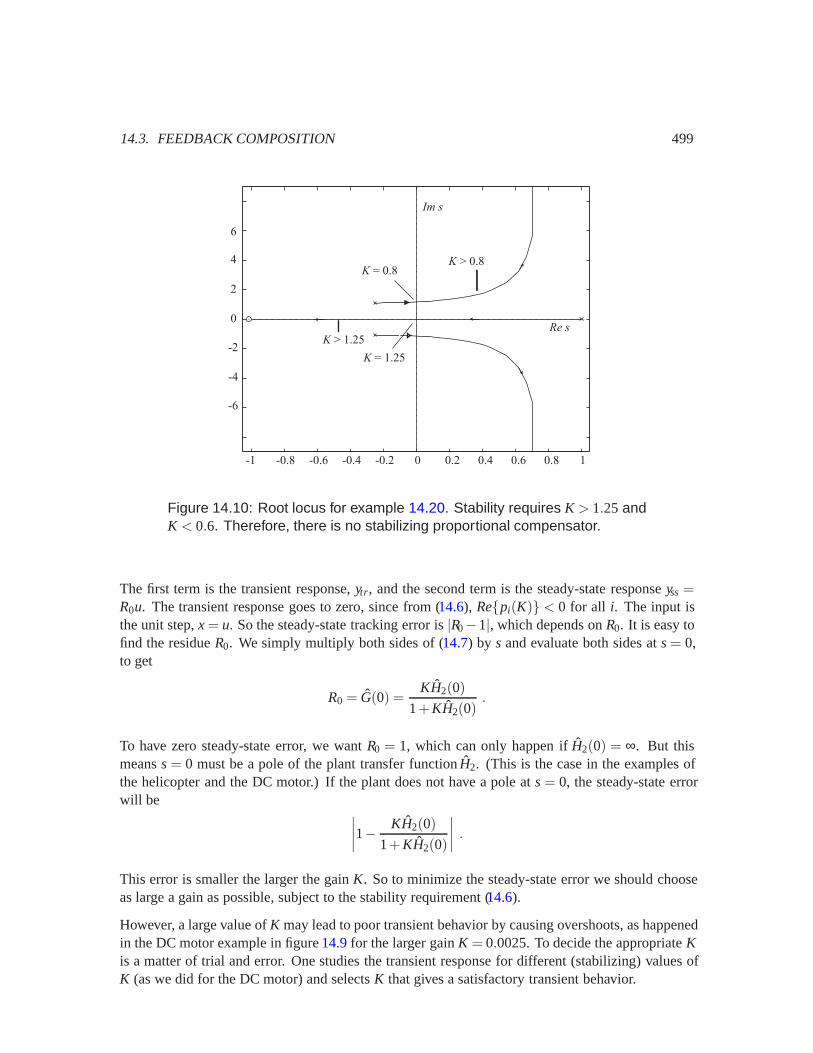
14.3. FEEDBACK COMPOSITION 499
-1 -0.8 -0.6 -0.4 -0.2 0 0.2 0.4 0.6 0.8 1
-4
-2
-6
2
4
6
0Re s
Im s
K = 1.25K > 1.25
K = 0.8K > 0.8
Figure 14.10: Root locus for example 14.20. Stability requires K > 1.25 andK < 0.6. Therefore, there is no stabilizing proportional compensator.
The first term is the transient response, ytr , and the second term is the steady-state response yss =R0u. The transient response goes to zero, since from (14.6), Re{pi(K)} < 0 for all i. The input isthe unit step, x = u. So the steady-state tracking error is |R0−1|, which depends on R0. It is easy tofind the residue R0. We simply multiply both sides of (14.7) by s and evaluate both sides at s= 0,to get
R0 = G(0) =KH2(0)
1+KH2(0).
To have zero steady-state error, we want R0 = 1, which can only happen if H2(0) = ∞. But thismeans s= 0 must be a pole of the plant transfer function H2. (This is the case in the examples ofthe helicopter and the DC motor.) If the plant does not have a pole at s= 0, the steady-state errorwill be ∣∣∣∣1− KH2(0)
1+KH2(0)
∣∣∣∣ .
This error is smaller the larger the gain K. So to minimize the steady-state error we should chooseas large a gain as possible, subject to the stability requirement (14.6).
However, a large value of K may lead to poor transient behavior by causing overshoots, as happenedin the DC motor example in figure 14.9 for the larger gain K = 0.0025. To decide the appropriate Kis a matter of trial and error. One studies the transient response for different (stabilizing) values ofK (as we did for the DC motor) and selects K that gives a satisfactory transient behavior.
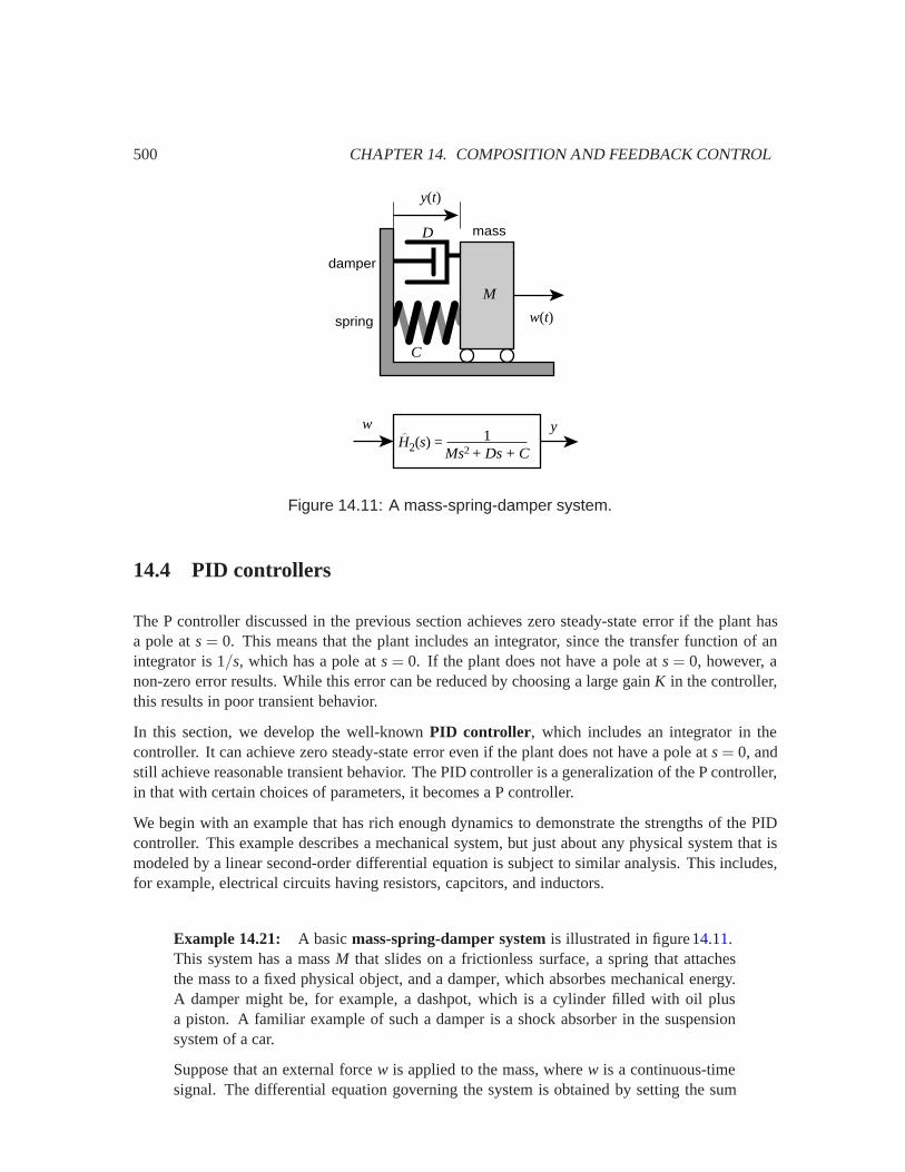
500 CHAPTER 14. COMPOSITION AND FEEDBACK CONTROL
w(t)
D
y(t)
M
C
spring
damper
mass
H2(s) =yw
1Ms2 + Ds + C
Figure 14.11: A mass-spring-damper system.
14.4 PID controllers
The P controller discussed in the previous section achieves zero steady-state error if the plant hasa pole at s= 0. This means that the plant includes an integrator, since the transfer function of anintegrator is 1/s, which has a pole at s= 0. If the plant does not have a pole at s= 0, however, anon-zero error results. While this error can be reduced by choosing a large gain K in the controller,this results in poor transient behavior.
In this section, we develop the well-known PID controller, which includes an integrator in thecontroller. It can achieve zero steady-state error even if the plant does not have a pole at s= 0, andstill achieve reasonable transient behavior. The PID controller is a generalization of the P controller,in that with certain choices of parameters, it becomes a P controller.
We begin with an example that has rich enough dynamics to demonstrate the strengths of the PIDcontroller. This example describes a mechanical system, but just about any physical system that ismodeled by a linear second-order differential equation is subject to similar analysis. This includes,for example, electrical circuits having resistors, capcitors, and inductors.
Example 14.21: A basic mass-spring-damper system is illustrated in figure 14.11.This system has a mass M that slides on a frictionless surface, a spring that attachesthe mass to a fixed physical object, and a damper, which absorbes mechanical energy.A damper might be, for example, a dashpot, which is a cylinder filled with oil plusa piston. A familiar example of such a damper is a shock absorber in the suspensionsystem of a car.
Suppose that an external force w is applied to the mass, where w is a continuous-timesignal. The differential equation governing the system is obtained by setting the sum
14.4. PID CONTROLLERS 501
of all forces to zero,My(t)+Dy(t)+Cy(t) = w(t).
The output y(t) is the position of the mass at time t, My(t) is the inertial force, Dy(t)is the damping force due to the damper, Cy(t) is the restoring force of the spring, andw(t) is the externally applied force. We assume that y(t) = 0 when the spring is in itsequilibrium position (neither extended nor compressed). M, D, and C are constants.Taking the Laplace transform, using the differentiation property from table13.4, gives
s2Y(s)+DsY(s)+CY(s) = W(s),
so the plant or open loop transfer function is
H2(s) =Y(s)W(s)
=1
Ms2 +Ds+C.
Suppose for example that the constants have values M = 1, D = 1,and C = 1.25. Then
H2(s) =1
s2 +s+ 1.25. (14.8)
In this case, the transfer function has a pair of complex poles at s = −0.5± i. Sincetheir real part is strictly negative, the system is stable.
Suppose we wish to drive the system to move the mass to the right one unit of distanceat time t = 0. We can apply an input force that is a unit step, scaled so that the steady-state response places the mass at position y(t) = 1. The final steady-state output isdetermined by the DC gain, which is H2(0) = 1/1.25 = 0.8, so we can apply an inputgiven by
∀ t, ,w(t) =1
0.8u(t) = 1.25u(t),
where u is the unit step signal. The resulting response yo has Laplace transform
Yo(s) =1
s2 +s+ 1.25· 1.25
s=−0.5+ 0.25i
s+ 0.5− i+−0.5−0.25i
s+ 0.5+ i+
1s
.
We call this the open-loop step response, because there is no control loop (yet).
Taking the inverse transform gives the open-loop step response
∀ t, yo(t) = e−0.5t [(−0.5+ 0.25i)eit +(−0.5−0.25i)e−it ]u(t)+u(t).
By combining the complex conjugate terms, this can be expressed as
∀t, yo(t) = Re−0.5t cos(t +θ)u(t)+u(t),
where R = 1.12 and θ = 2.68. Figure 14.12 displays a plot of this open-loop stepresponse yo. Notice that the mass settles to position y(t) = 1 for large t.
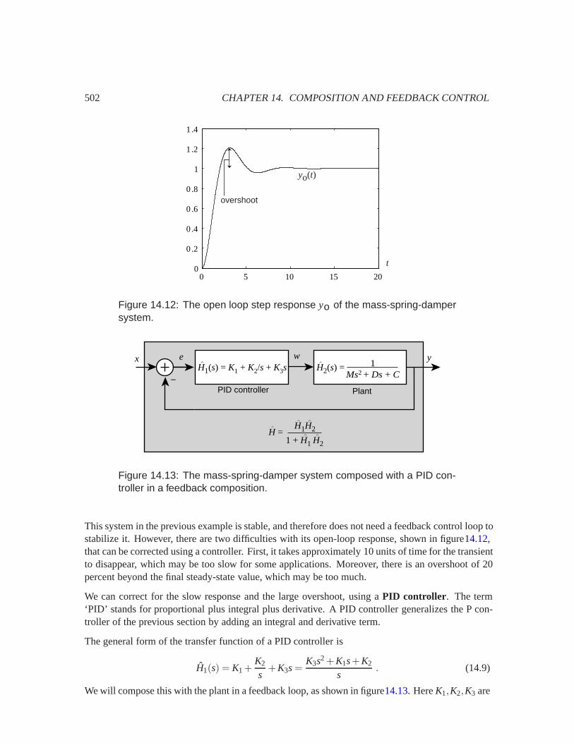
502 CHAPTER 14. COMPOSITION AND FEEDBACK CONTROL
yo(t)
t
overshoot
0 5 10 15 200
0 .2
0 .4
0 .6
0 .8
1
1 .2
1 .4
Figure 14.12: The open loop step response yo of the mass-spring-dampersystem.
x e y
H =H1H2
1 + H1 H2
−H2(s) =
w1
Ms2 + Ds + CH1(s) = K1 + K2/s + K3s
PID controller Plant
Figure 14.13: The mass-spring-damper system composed with a PID con-troller in a feedback composition.
This system in the previous example is stable, and therefore does not need a feedback control loop tostabilize it. However, there are two difficulties with its open-loop response, shown in figure14.12,that can be corrected using a controller. First, it takes approximately 10 units of time for the transientto disappear, which may be too slow for some applications. Moreover, there is an overshoot of 20percent beyond the final steady-state value, which may be too much.
We can correct for the slow response and the large overshoot, using a PID controller. The term‘PID’ stands for proportional plus integral plus derivative. A PID controller generalizes the P con-troller of the previous section by adding an integral and derivative term.
The general form of the transfer function of a PID controller is
H1(s) = K1 +K2
s+K3s=
K3s2 +K1s+K2
s. (14.9)
We will compose this with the plant in a feedback loop, as shown in figure14.13. Here K1,K2,K3 are
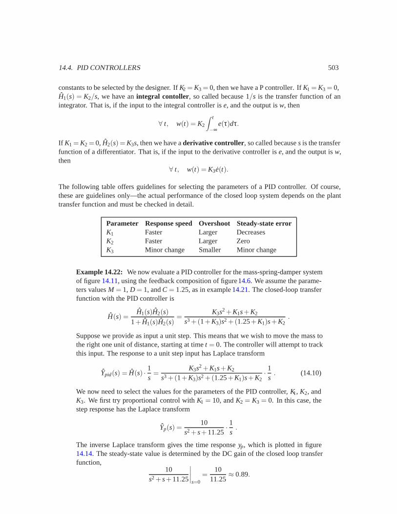
14.4. PID CONTROLLERS 503
constants to be selected by the designer. If K2 = K3 = 0, then we have a P controller. If K1 = K3 = 0,H1(s) = K2/s, we have an integral contoller, so called because 1/s is the transfer function of anintegrator. That is, if the input to the integral controller is e, and the output is w, then
∀ t, w(t) = K2
∫ t
−∞e(τ)dτ.
If K1 = K2 = 0, H2(s) = K3s, then we have a derivative controller, so called because s is the transferfunction of a differentiator. That is, if the input to the derivative controller is e, and the output is w,then
∀ t, w(t) = K3e(t).
The following table offers guidelines for selecting the parameters of a PID controller. Of course,these are guidelines only—the actual performance of the closed loop system depends on the planttransfer function and must be checked in detail.
Parameter Response speed Overshoot Steady-state errorK1 Faster Larger DecreasesK2 Faster Larger ZeroK3 Minor change Smaller Minor change
Example 14.22: We now evaluate a PID controller for the mass-spring-damper systemof figure 14.11, using the feedback composition of figure14.6. We assume the parame-ters values M = 1, D = 1, and C = 1.25, as in example 14.21. The closed-loop transferfunction with the PID controller is
H(s) =H1(s)H2(s)
1+ H1(s)H2(s)=
K3s2 +K1s+K2
s3 +(1+K3)s2 +(1.25+K1)s+K2.
Suppose we provide as input a unit step. This means that we wish to move the mass tothe right one unit of distance, starting at time t = 0. The controller will attempt to trackthis input. The response to a unit step input has Laplace transform
Ypid(s) = H(s) · 1s
=K3s2 +K1s+K2
s3 +(1+K3)s2 +(1.25+K1)s+K2· 1
s. (14.10)
We now need to select the values for the parameters of the PID controller, K1, K2, andK3. We first try proportional control with K1 = 10, and K2 = K3 = 0. In this case, thestep response has the Laplace transform
Yp(s) =10
s2 +s+ 11.25· 1
s.
The inverse Laplace transform gives the time response yp, which is plotted in figure14.14. The steady-state value is determined by the DC gain of the closed loop transferfunction,
10s2 +s+ 11.25
∣∣∣∣s=0
=10
11.25≈ 0.89.

504 CHAPTER 14. COMPOSITION AND FEEDBACK CONTROL
0 2 4 6 8 10 12 14 16 18 200
0.5
1
1.5
yo
yp
ypd
ypid
Figure 14.14: The step response for open loop, yo, with P-control, yp, PD-control, ypd, and PID-control, ypid .
14.5. SUMMARY 505
This yields an error of 11 percent, and the overshoot of 50 percent is much worse thanthat of the open-loop response yo, also shown in the figure. Thus, a P controller withgain K = 10 is useless for this application.
Following the guidelines in the table above, we add derivative control to reduce theovershoot. The result is a so-called PD controller, because it adds a proportional anda derivative term. For the PD controller we choose K1 = 10 and K3 = 10. Substitutionin (14.10) gives the Laplace transform of the step response,
Ypd(s) =10s+ 10
s2 + 11s+ 11.25· 1
s.
The steady-state value is given by the DC gain of the closed loop transfer function,
10s+ 10s2 + 11s+ 11.25
∣∣∣∣s=0≈ 0.89,
which is the same as the steady-state value for the P controller. The inverse Laplacetransform gives the time response ypd, which is plotted in figure 14.14. The overshootis reduced to 10 percent—a large improvement. Also, the response is quicker—thetransient disappears in about 4 time units.
Finally, to eliminate the steady-state error we add integral control. For the PID con-troller we choose K1 = 10,K2 = 5,K3 = 10. Substitution in (14.10) gives the Laplacetransform of the step response
Ypid(s) =10s2 + 10s+ 5
s3 + 11s2 + 11.25s+ 5· 1
s.
The steady-state value is again given by the DC gain of the closed loop transfer func-tion,
10s2 + 10s+ 5s3 + 11s2 + 11.25s+ 5
∣∣∣∣s=0
= 1.
So the steady-state error is eliminated, as expected. The time response ypid is plottedin figure 14.14. It shows significant improvement over the other responses. There isno overshoot, and the transient disappears in about 4 time units. Further tuning of theparameters K1,K2,K3 could yield small improvements.
14.5 Summary
This chapter considers cascade, parallel, and feedback compositions of LTI systems described byZ or Laplace transforms. Cascade composition is applied to equalization, parallel composition isapplied to noise cancellation, and feedback composition is applied to control.
Because we are using Z and Laplace transforms rather than Fourier transforms, we are able to con-sider unstable systems. In particular, we find that while, in principle, cascade and parallel composi-tions can be used to stabilize unstable systems, the result is not robust. Small changes in parameter

506 CHAPTER 14. COMPOSITION AND FEEDBACK CONTROL
values can result in the system being once again unstable. Feedback composition, on the other hand,can be used to robustly stabilize unstable systems. We illustrate this first with a simple helicopterexample. The second example, a DC motor, benefits from more sophisticated controllers. Thethird example, a mass-spring-damper system, motivates the development of the well-known PIDcontroller structure. PID controllers can be used to stabilize unstable systems and to improve theresponse time, precision, and overshoot of stable systems.
Exercises
Each problem is annotated with the letter E, T, C which stands for exercise, requires some thought,requires some conceptualization. Problems labeled E are usually mechanical, those labeled T re-quire a plan of attack, those labeled C usually have more than one defensible answer.
1. E This exercise studies equalization when the channel is only known approximately. Considerthe cascade composition of figure 14.1, where H1 is the channel to be equalized, and H2 is theequalizer. If the equalizer is working perfectly, then x = y. For example, if
H1(z) =z
z−0.5and H2(z) =
z−0.5z
,
then x = y because H1(z)H2(z) = 1.
(a) Suppose that H2(z) is as given above, but the plant is a bit different,
H1(z) =z
z−0.5− ε.
Suppose that x = δ, the Kronecker delta function. Plot y−x for ε = 0.1 and ε =−0.1.
(b) Now suppose that the equalizer is
H2(z) =z−2
z,
and the channel isH1(z) =
zz−2− ε
.
Again suppose that x = δ, the Kronecker delta function. Plot y−x for ε = 0.1,−0.1.
(c) For part (b), show that equalization error y− x grows without bound whenever ε �= 0,|ε|< 1.
2. E This exercise studies equalization for continuous-time channels. Consider the cascade com-position of figure 14.1, where H1 is the channel to be equalized, and H2 is the equalizer. Bothare causal. If
H1(s) =s+ 1s+ 2
and H2(s) =s+ 2s+ 1
,
then x = y because H1(s)H2(s) = 1.
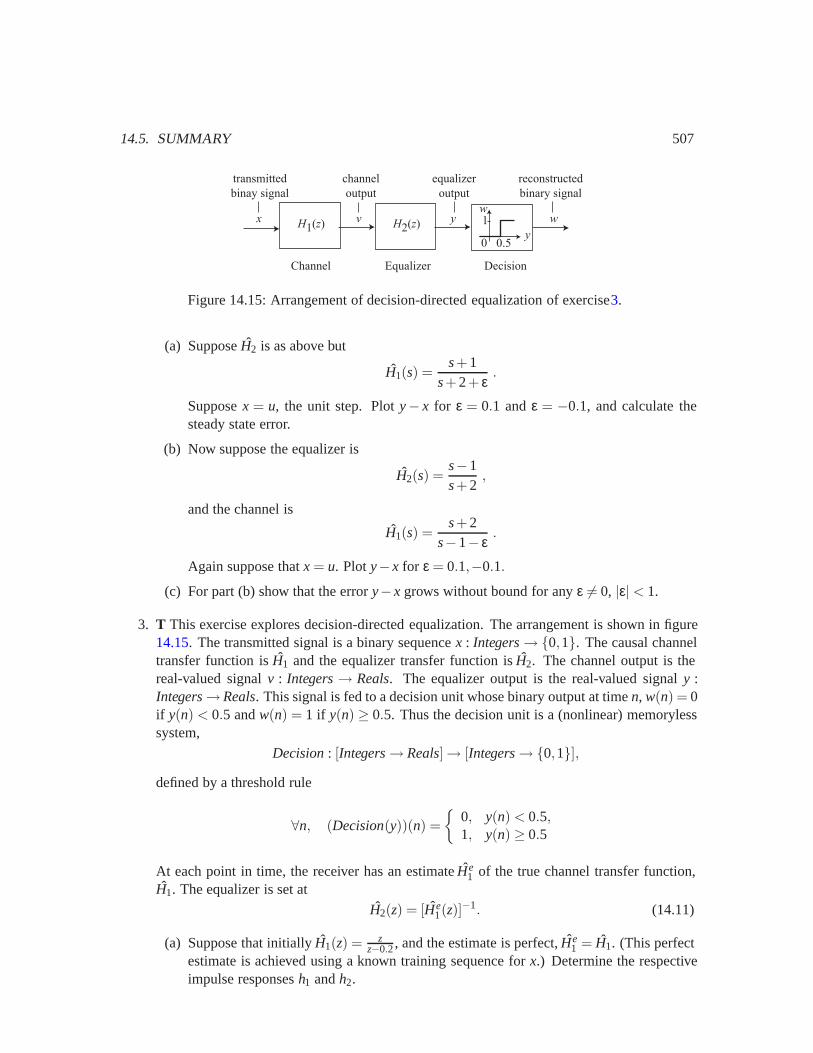
14.5. SUMMARY 507
x v y wy
w
0.50
1H1(z) H2(z)
Channel Equalizer Decision
transmittedbinay signal
equalizeroutput
reconstructedbinary signal
channeloutput
Figure 14.15: Arrangement of decision-directed equalization of exercise3.
(a) Suppose H2 is as above but
H1(s) =s+ 1
s+ 2+ ε.
Suppose x = u, the unit step. Plot y− x for ε = 0.1 and ε = −0.1, and calculate thesteady state error.
(b) Now suppose the equalizer is
H2(s) =s−1s+ 2
,
and the channel is
H1(s) =s+ 2
s−1− ε.
Again suppose that x = u. Plot y−x for ε = 0.1,−0.1.
(c) For part (b) show that the error y−x grows without bound for any ε �= 0, |ε|< 1.
3. T This exercise explores decision-directed equalization. The arrangement is shown in figure14.15. The transmitted signal is a binary sequence x : Integers→ {0,1}. The causal channeltransfer function is H1 and the equalizer transfer function is H2. The channel output is thereal-valued signal v : Integers→ Reals. The equalizer output is the real-valued signal y :Integers→Reals. This signal is fed to a decision unit whose binary output at time n, w(n) = 0if y(n) < 0.5 and w(n) = 1 if y(n) ≥ 0.5. Thus the decision unit is a (nonlinear) memorylesssystem,
Decision: [Integers→ Reals]→ [Integers→ {0,1}],defined by a threshold rule
∀n, (Decision(y))(n) ={
0, y(n) < 0.5,1, y(n) ≥ 0.5
At each point in time, the receiver has an estimate He1 of the true channel transfer function,
H1. The equalizer is set at
H2(z) = [He1(z)]−1. (14.11)
(a) Suppose that initially H1(z) = zz−0.2 , and the estimate is perfect, He
1 = H1. (This perfectestimate is achieved using a known training sequence for x.) Determine the respectiveimpulse responses h1 and h2.
508 CHAPTER 14. COMPOSITION AND FEEDBACK CONTROL
Now suppose the signal x is
∀n, x(n) =
0, n < 01, n≥ 0,n even0, n≥ 0,n odd
(14.12)
Calculate the channel output v(n) = (h1 ∗ x)(n),n ≤ 3. Then calculate the equalizeroutput y(n) = (h2 ∗ v)(n),n ≤ 3, and check that y(n) = x(n),n ≤ 3. Also check thatw(n) = x(n),n≤ 3.
(b) Now suppose the channel transfer function has changed to
H1(z) =z
z−0.3,
but the receiver’s estimate hasn’t changed, i.e.
He1(z) =
zz−0.2
,
so the equalizer (14.11) hasn’t change either. For the same input signal again calculatethe channel and equalizer outputs v(n),y(n),n≤ 3. Check that y(n) �= x(n),n > 0. Butshow that the decision w(n) = x(n),n≤ 3. So the equalizer correctly determines x.
(c) Since the receiver’s decision w = x, it can make a new estimate of the channel using thefact that Y = H1H2X = H1H2W. The new estimate is
He1 =
Y
H2W. (14.13)
Suppose time is 3, and the receiver has observed y(n),w(n),n≤ 3. Since the Z trans-forms Y and W also depend on values of y(n),w(n) for n> 3, these Z transforms can notbe calculated at time n = 3, and so the estimator (14.13) cannot be used. The followingapproach will work, however.
Suppose the receiver knows that the unknown channel transfer function is of the form
H1(z) =z
z−a,
so that only the parameter a has to be estimated. Using this information, we have
Y(z) =z
z−az−0.2
zW(z) =
z−0.2z−a
W(z).
Now take the inverse Z transform and express the time-domain relation between y andw. Show that you can estimate a knowing y(0),y(1),w(0),w(1).
4. E This continues exercise 3. It shows that if the channel estimate He1 is not sufficiently close
to the true channel H1, the decision may become incorrect. Suppose the true channel isH1(z) = z
z−a, the estimate is He1(z) = z
z−0.2 , the equalizer is H2(z) = [He1(z)]−1 = z−0.2
z , andthe decision is as in figure 14.15. Assume the input signal x to be the same as in (14.12) Showthat if a = 0.6 then w(0) = x(0),w(1) = x(1),w(2) = x(2), but w(3) �= x(3).

14.5. SUMMARY 509
5. E This exercise continues the discussion in examples 14.5, 14.6 for the continuous-time,causal and stable channel with impulse response h1 and transfer function
∀s∈ RoC(h1) = {s | Re{s} >−1}, H1(s) =s−2s+ 1
.
(a) Calculate h1 and sketch it. (Observe how the zero in the right-half plane at s= 2 accountsfor the negative values.)
(b) The inverse of H1,
H2(s) =s+ 1s−2
,
has a pole at s= 2. So as a causal system, the inverse is unstable. But as a non-causalsystem, it is stable with RoC= {s | Re{s} < 2} which includes the imaginary axis.Evaluate the impulse response h2 of H2 as an anti-causal system, and give a sketch.
(c) The impulse response h2 calculated in (a) is non-zero for t ≤ 0. Consider the finite-duration, anti-causal impulse response h3 obtained by truncating h2 before time -5,
∀t ∈ Reals, h3(t) ={
h2(t), t ≥−50, t <−5
and sketch h3. Calculate the transfer function H3, including its RoC, by using the defi-nition of the Laplace transform.
(d) Obtain the causal impulse response h4 by delaying h3 by time T, i.e.
∀t ∈ Reals, h4(t) = h3(t +T).
Sketch h4 and find its transfer function, H4. Then H4 is an approximate inverse of H1
with a delay of 5 time units. (Note: h3 has a delta function at 0.)
6. T The proportional controller of figure 14.7 stabilizes the plant for K > 1. In this exercise,we try to achieve the same effect by the cascade compensator of figure14.1.
(a) Assume that the plant H2 is as given in figure 14.7. Design H1 for the cascade composi-tion of figure 14.1 so that H2H1 is the same as the closed-loop transfer function achievedin figure 14.7.
(b) Now suppose that the model of the plant is not perfect, and the plant’s real transferfunction is
H2(s) =1
M(s− ε),
for some small value of ε > 0. Using the same H1 that you designed in part (a), what isthe transfer function of the cascade composition? Is it stable?
7. T Consider a discrete-time causal plant with transfer function
H2(z) =z
z−2.
(a) Where are the poles and zeros? Is the plant stable?

510 CHAPTER 14. COMPOSITION AND FEEDBACK CONTROL
(b) Find the impulse response of the plant. Is it bounded?
(c) Give the closed-loop transfer function for the P controller for this plant.
(d) Sketch the root locus for the P controller for this plant.
(e) For what values of K is the closed-loop system stable?
(f) Find the step response of the closed-loop system. Identify the transient and steady-stateresponses. For K = 10, what is the steady-state tracking error?
(g) Suppose that the plant is instead given by
H2 =z
z−2− ε,
for some real ε ≥ 0. For what values of K is the P controller robust for plants with|ε|< 0.5?
8. T Consider the feedback composition in figure14.6. Suppose that H1H2 is causal and strictlyproper, meaning that the order of the numerator is greater than the order of the denominator.
(a) Show that if H1H2 is causal and strictly proper, then so is H, the transfer function of thefeedback composition given by (14.1).
(b) For the discrete-time case, show that we can write
H1(z)H2(z) = z−1G(z), (14.14)
where G(z) is proper, and is the transfer function of a causal system. Intuitively, thismeans that there must be a net unit delay in the feedback loop, because z−1 is the transferfunction of a unit delay.
(c) Use the result of part (a) to argue that the system H1H2 has state-determined output.
(d) For the continuous-time case, show that we can write
H1(s)H2(s) = s−1G(s), (14.15)
where G(s) is proper, and is the transfer function of a causal system. Intuitively, thismeans that there must be an integration in the feedback loop, because s−1 is the transferfunction of an integrator.
(e) Use the result of part (c) to argue that the system H1H2 has state-determined output,assuming that the input is bounded and piecewise continuous.
9. E Consider the mth order polynomial sN + am−1sm−1 + · · ·+ a1s+ a0. Suppose all its rootshave negative real parts. Show that all coefficients of the polynomial must be positive, i.e.,am−1 > 0, · · · ,a0 > 0. Hint. Express the polynomial as (s− p1) · · · (s− pm) with Re{pi} > 0.Note that complex roots must occur in complex conjugate pairs. (The positiveness of allcoefficients is a necessary condition. A sufficient condition is given by the Routh-Hurwitzcriterion, described in control theory texts.)
10. T Consider the feedback composition in figure 14.6. The plant’s transfer function is H2(s) =1/s2.

14.5. SUMMARY 511
(a) Show that no PI controller in the form H1(s) = K1 +K2/s can stabilize the closed loopsystem for any values of K1,K2. Hint. Use the result of problem 9.
(b) Show that by the proper choice of the coefficients K1,K2 of a PD controller in the formH1(s) = K1 + K2s, you can place the closed-loop poles at any locations p1, p2 (thesemust be complex conjugate if they are complex).
11. T Consider the feedback composition in figure 14.6. The plant’s transfer function is H2(s) =1/(s2 + 2s+ 1). The PI controller is H1(s) = K1 +K2/s.
(a) Take K2 = 0, and plot the root locus as K1 varies. For what values of K1 is the closedloop system stable? What is the steady state error to a step input as a function of K1?
(b) Select K1,K2 such that the closed loop system is stable and has zero-steady state error.