stability results for the time-harmonic maxwell equations

Stability results for the time-harmonic Maxwell equations with impedance boundary conditions Article

Accepted Version

Hiptmair, R., Moiola, A. and Perugia, I. (2011) Stability results for the time-harmonic Maxwell equations with impedance boundary conditions. Mathematical models and methods in applied Sciences (M3AS), 21 (11). pp. 2263-2287. ISSN 0218-2025 doi: https://doi.org/10.1142/S021820251100574X Available at https://centaur.reading.ac.uk/28024/

It is advisable to refer to the publisher’s version if you intend to cite from the work. See Guidance on citing .

To link to this article DOI: http://dx.doi.org/10.1142/S021820251100574X

Publisher: World Scientific

All outputs in CentAUR are protected by Intellectual Property Rights law, including copyright law. Copyright and IPR is retained by the creators or other copyright holders. Terms and conditions for use of this material are defined in the End User Agreement .

www.reading.ac.uk/centaur

CentAUR

http://centaur.reading.ac.uk/71187/10/CentAUR%20citing%20guide.pdf

http://www.reading.ac.uk/centaur

http://centaur.reading.ac.uk/licence

Central Archive at the University of Reading Reading’s research outputs online

November 11, 2010 10:24 WSPC/INSTRUCTION FILE mainM3AS

Mathematical Models and Methods in Applied Sciencesc© World Scientific Publishing Company

STABILITY RESULTS FOR THE TIME-HARMONIC MAXWELL

EQUATIONS WITH IMPEDANCE BOUNDARY CONDITIONS

RALF HIPTMAIR

Seminar for Applied Mathematics, ETH Zurich, Ramistrasse 101

8092 Zurich, Switzerland

[email protected]

ANDREA MOIOLA

Seminar for Applied Mathematics, ETH Zurich, Ramistrasse 101

8092 Zurich, Switzerland

[email protected]

ILARIA PERUGIA

Department of Mathematics, University of Pavia, Via Ferrata 1

27100 Pavia, Italy

[email protected]

Received (Day Month Year)Revised (Day Month Year)

Communicated by (xxxxxxxxxx)

We consider the time-harmonic Maxwell equations with constant coefficients in abounded, uniformly star-shaped polyhedron. We prove wavenumber-explicit normbounds for weak solutions. This result is pivotal for convergence proofs in numericalanalysis and may be a tool in the analysis of electromagnetic boundary integral opera-tors.

Keywords: Time-harmonic Maxwell’s equations; impedance boundary conditions; stabil-ity estimates; regularity.

AMS Subject Classification: 35B65, 35D30, 35Q61

1. Introduction

Stability estimates of variational solutions to PDE’s with stability constants which

are explicit in some of the characteristic parameters are important in the theoreti-

cal analysis, and then in the design, of discretization methods. Often, discretization

parameters have to be chosen in relation to the physical ones, in order to design ac-

curate, robust, and efficient numerical methods. This is the case for time-harmonic

wave propagation problems, where the choice of the discretization parameters in

relation to the wavenumber is crucial. There, fundamental model problems con-

sider bounded domains with piecewise smooth boundary and first order absorbing

1


2 R. Hiptmair, A. Moiola, I. Perugia

boundary conditions (impedance boundary conditions, IBC).

For the Helmholtz problem with IBC, stability estimates in weighted H1–norm

with explicit dependence on the wavenumber were derived in Proposition 8.1.4

of [17] in the 2D case, then extended to the 3D case, with a similar argument, in [7]

and [11]; in the latter reference, the case of mixed boundary conditions was also

considered. In these results, in order to use Rellich identities, the problem domain

is assumed to be star-shaped with respect to a ball; a key ingredient in the proof is

the fact that the weak solution is smoother than merely H1, which holds true for

polygonal/polyhedral domains.

For the time-harmonic Maxwell equations with IBC, stability estimates were

derived with a Fredholm-type argument in [18, Theorem 4.17]. Unfortunately, this

analysis does not allow to establish how the stability constant depends on the

wavenumber. The main obstacle to extending the argument of [17] to the Maxwell

case consists in the poor regularity of the analytical solutions, even in the case of

constant material coefficients. In fact, while for Dirichlet boundary conditions, the

solution always has H1–regularity in convex domains, for IBC, H1–regularity is

guaranteed only for smooth domains (see [8]).

In this paper, we consider the time-harmonic Maxwell equations with constant

coefficients in bounded, uniformly star-shaped domains. In Section 3, stability esti-

mates in a weighted H(curl)–norm are derived. For smooth domains, relying upon

the regularity results established in [8], we extend the argument of [17] and prove

stability with constants independent of the wavenumber (see Theorem 3.1). Then,

with a technique similar to that of [10, Thm. 3.2.1.3], we extend this result to

polyhedral domains (see Theorem 3.2).

For the analysis of numerical approximations of Maxwell solutions, which relies

on duality arguments, it is also interesting to derive elliptic regularity results. For

this reason, in Section 4 (see Theorem 4.4), we prove that, provided that the bound-

ary data are in Hs′

, 0 < s′ < 1/2, the solutions reach a regularity H1/2+s, for some

0 < s ≤ s′ < 1/2, in polyhedral domains. In a convex polyhedron, the regularity is

always optimal: s = s′ < 1/2. The constant in the stability estimates in stronger

norms (H1 for smooth domains, H1/2+s for polyhedral domains) linearly depends

on the wavenumber.

Our main reason of interest in these stability and regularity results was their

application in the error analysis of Trefftz-discontinuous Galerkin approximations

of the time-harmonic Maxwell equations. In fact, in [13], we are extending to the

Maxwell case the theory developed in [14] for the Helmholtz problem, where uniform

stability with respect to the wavenumber, together with elliptic regularity, played

an essential role. Another potential application is the extension to electromagnetic

waves of the norm and stability bounds of boundary integral operators for acoustic

scattering derived in [6] and [23].

We conclude this introduction by setting some notation used throughout this

paper. If D is a domain in R2 or R3, we denote by Hk(D)d, d = 1, 2, 3, the Sobolev


Stability Results for the Time-Harmonic Maxwell Equations 3

space with integer or fractional regularity index k and values in Cd, and by ‖·‖k,Ω

the corresponding Sobolev norm; we denote by H10 (D) the closure in H1(D) of

C∞0 (D) and set L2(D) = H0(D).

For D ⊂ R3, we introduce the following Hilbert spaces, see also [9, Ch. 1],

H(curl;D) = v ∈ L2(D)3 : ∇× v ∈ L2(D)3 ,H(div;D) = v ∈ L2(D)3 : ∇ · v ∈ L2(D) ,H(div0;D) = v ∈ L2(D)3 : ∇ · v = 0 in D ,L2

T (∂D) := v ∈ L2(∂D)3 : v · n = 0 ,

endowed with the corresponding graph norms.

If D is a Lipschitz domain in R3 and n is the exterior unit normal vector field to

∂D, the following integration by parts formula holds true for functions inH(curl;D):∫

D

∇× F · G dV =

∫

D

F · ∇ × G dV +

∫

∂D

n × F · G dS ,

provided that the second integral on the right-hand side is intended as a duality

product between the appropriate trace spaces (see [3]). If D is a vector-valued

function defined in D, we denote its normal and tangential components on ∂D by

DN := (D · n)n and DT := (n × D) × n, respectively.

Finally, we write Br(x0) for the (open) ball of radius r centered at x0 and by

S2 = x ∈ R3 : |x| = 1 the unit sphere.

2. The Maxwell boundary value problem

Let Ω ⊂ R3 be an open bounded domain, which is either has a C2 boundary or is

a polyhedron. We assume that

there exist a point x0 ∈ Ω and a real number γ > 0 for which Ω is

star-shaped with respect to all points in Bγ(x0).

For each point x ∈ ∂Ω, the open cone with vertex x, height |x − x0| and opening

angle θ = arctan(γ/|x − x0|) > arctan(γ/ diam(Ω)) is contained in Ω. This means

that the domain satisfies the uniform cone condition; therefore, by [10, Thm. 1.2.2.2],

Ω is Lipschitz.

We consider the following frequency-domain formulation of the Maxwell equa-

tions in terms of electric field E and magnetic field H with impedance boundary

conditions in the domain Ω:

−iωǫ E −∇× H = −J/iω in Ω ,

−iωµ H + ∇× E = 0 in Ω ,

H × n − λ(n × E) × n = g/iω on ∂Ω ,

(2.1)

where ω > 0 is a fixed wave number, J ∈ H(div0; Ω) is related to a given current

density, and g ∈ L2T (∂Ω). The material coefficients



ǫ, µ, λ ∈ R are assumed to be constant

with ǫ, µ > 0 and λ 6= 0.

By expressing H in terms of E using the second equation of (2.1) and replacing

into the first equation and into the boundary condition, we obtain∇× (µ−1∇× E) − ω2ǫ E = J in Ω ,

(µ−1∇× E) × n − iωλ(n × E) × n = g on ∂Ω .(2.2)

Introducing the “energy space” (equipped with graph norm)

Himp(curl; Ω) = v ∈ H(curl; Ω) : vT ∈ L2T (∂Ω) ,

the variational formulation of the Maxwell problem (2.2) reads as follows: find

E ∈ Himp(curl; Ω) such that, for all ξ ∈ Himp(curl; Ω), it holds

A(E, ξ) =

∫

Ω

J · ξ dV +

∫

∂Ω

g · ξT dS , (2.3)

where

A(E, ξ) :=

∫

Ω

[(µ−1∇× E) · (∇× ξ) − ω2(ǫE) · ξ

]dV − iω

∫

∂Ω

λET · ξT dS .

Well-posedness of problem (2.3) in Himp(curl; Ω) is proved in [18, Thm. 4.17]

that we report here.

Theorem 2.1. Under the assumptions made on Ω, J , g and on the material coef-

ficients, there exists a unique E ∈ Himp(curl; Ω) with ∇· (ǫE) = 0 solution to (2.3).

3. Stability estimates

In this section, we prove stability estimates in energy-norm for problem (2.3), with

stability constants independent of the wave number ω.

We use the argument developed in [17, Sect. 8.1] (see also [7] and [11]) for

the Helmholtz problem. In order to do that, we have to choose a particular test

functions, the admissibility of which requires some smoothness of the Maxwell solu-

tion. Therefore, we will proceed in two steps: in Section 3.1, following [17, Proof of

Prop. 8.1.4] and [11], we prove stability estimates for problem (2.3) for C2–domains

(see Theorem 3.1). Then, in Section 3.2, we extend this result to non-smooth do-

mains (see Theorem 3.2). Before doing that, we establish the following geometric

equivalence.

Lemma 3.1. Let Ω ⊂ R3 be a bounded, either C2 or polyhedral domain. Then Ω

is star-shaped with respect to Bγ(x0) if and only if, for all x ∈ ∂Ω for which n(x)

is defined, (x − x0) · n(x) ≥ γ.

Proof. Set Γ := x ∈ ∂Ω : n(x) is defined; our assumptions on Ω imply that

∂Ω \ Γ has zero 2–measure.



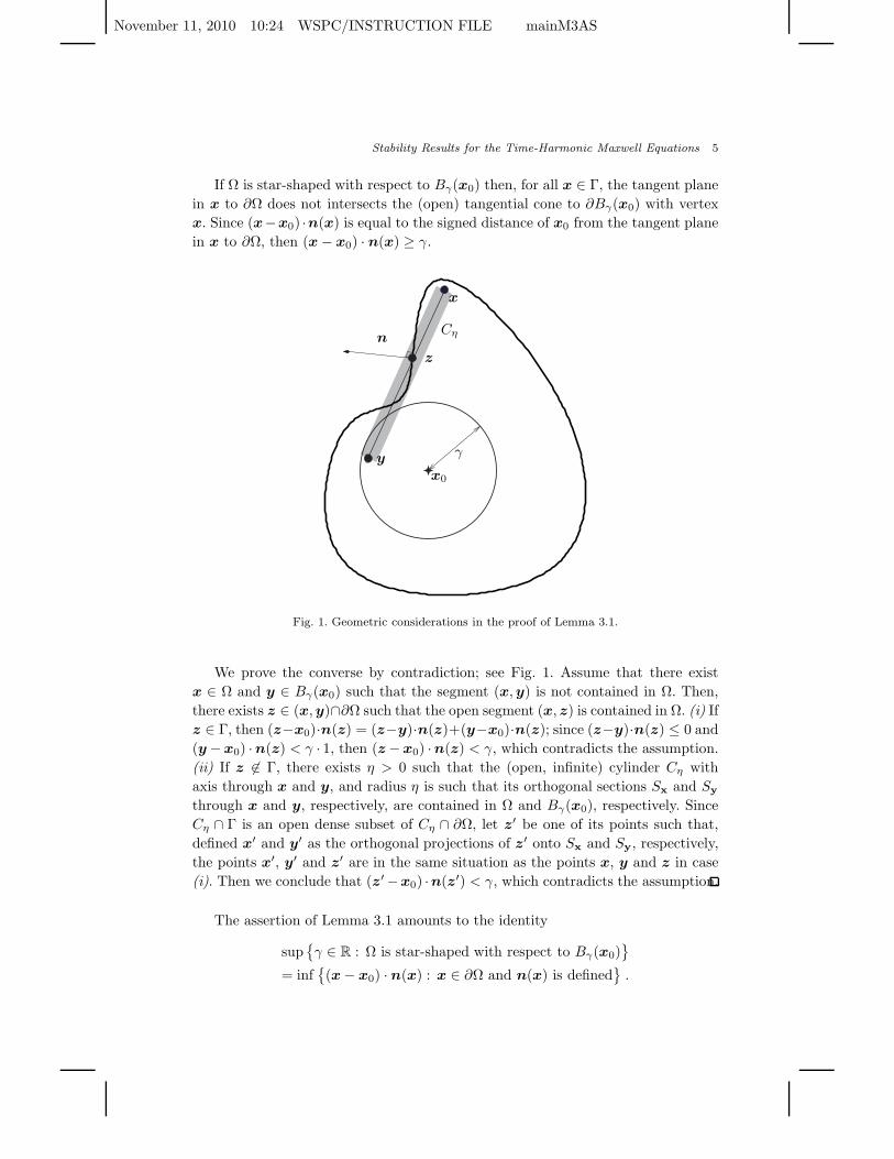
If Ω is star-shaped with respect to Bγ(x0) then, for all x ∈ Γ, the tangent plane

in x to ∂Ω does not intersects the (open) tangential cone to ∂Bγ(x0) with vertex

x. Since (x−x0) ·n(x) is equal to the signed distance of x0 from the tangent plane

in x to ∂Ω, then (x − x0) · n(x) ≥ γ.

x

y

z

Cη

γ

n

x0

Fig. 1. Geometric considerations in the proof of Lemma 3.1.

We prove the converse by contradiction; see Fig. 1. Assume that there exist

x ∈ Ω and y ∈ Bγ(x0) such that the segment (x,y) is not contained in Ω. Then,

there exists z ∈ (x,y)∩∂Ω such that the open segment (x, z) is contained in Ω. (i) If

z ∈ Γ, then (z−x0)·n(z) = (z−y)·n(z)+(y−x0)·n(z); since (z−y)·n(z) ≤ 0 and

(y −x0) ·n(z) < γ · 1, then (z −x0) ·n(z) < γ, which contradicts the assumption.

(ii) If z 6∈ Γ, there exists η > 0 such that the (open, infinite) cylinder Cη with

axis through x and y, and radius η is such that its orthogonal sections Sx and Sy

through x and y, respectively, are contained in Ω and Bγ(x0), respectively. Since

Cη ∩ Γ is an open dense subset of Cη ∩ ∂Ω, let z′ be one of its points such that,

defined x′ and y′ as the orthogonal projections of z′ onto Sx and Sy, respectively,

the points x′, y′ and z′ are in the same situation as the points x, y and z in case

(i). Then we conclude that (z′−x0) ·n(z′) < γ, which contradicts the assumption.

The assertion of Lemma 3.1 amounts to the identity

supγ ∈ R : Ω is star-shaped with respect to Bγ(x0)

= inf(x − x0) · n(x) : x ∈ ∂Ω and n(x) is defined

.



3.1. Stability for smooth domains

In this section, we consider the case of C2–domains. This ensures that all the Sobolev

spaces Hs(∂Ω), −2 < s < 2, and their tangential vectorial counterparts HsT (∂Ω) :=

ϕ ∈ Hs(∂Ω)3 : ϕ · n = 0 are well defined (see [1, p. 825]).

In order to prove stability estimates for problem (2.3), we need the following

regularity result proved in [8, Sect. 4.5.d]a. We report here the proof for the sake of

completeness.

Lemma 3.2. Let Ω ⊂ R3 be a bounded C2–domain. In addition to the assump-

tions made on J, g and on the material coefficients in Section 2, we assume

g ∈ H1/2T (∂Ω). Then, the solution E to problem (2.3) belongs to H1(curl; Ω) :=

v ∈ H1(Ω)3 : ∇× v ∈ H1(Ω)3.

Proof. Decompose E as

E = ΦΦΦ0 + ∇ψ ,where ΦΦΦ0 ∈ H1(Ω) ∩ H(div0; Ω) and ψ ∈ H1(Ω) (see [12, Lemma 2.4]); clearly,

∆ψ = 0 in Ω. By using this decomposition, we can write the boundary condition in

problem (2.3) by

(µ−1∇× E) × n − iωλΦΦΦ0T − iωλ∇Tψ = g on ∂Ω ,

where ∇Tψ is the tangential gradient of ψ, i.e., ∇Tψ := (n ×∇ψ) × n.

Using the results of [3] (see also [18, eq. (3.52)]), the tangential divergence

divT of (µ−1∇× E) × n is well-defined, belongs to H−1/2(∂Ω). Moreover, ΦΦΦ0T , g ∈

H1/2(∂Ω)3, and thus divT (λΦΦΦ0T + g) ∈ H−1/2(∂Ω). It follows that divT λ∇Tψ ∈

H−1/2(∂Ω) and, by an elliptic lifting theorem for the Laplace-Beltrami operator on

smooth surfaces, we find ψ ∈ H3/2(∂Ω); this, together with ∆ψ = 0 in Ω, gives

ψ ∈ H2(Ω), due to the smoothness of ∂Ω, which implies E ∈ H1(Ω)3.

Similarly, we prove the smoothness of ∇× E: decompose ∇× E as

∇× E = ΨΨΨ0 + ∇φwhere ΨΨΨ0 ∈ H1(Ω)3 ∩ H(div0; Ω), and φ ∈ H1(Ω); again, ∆φ = 0 in Ω. The

boundary condition in problem (2.3) can be written as

µ−1ΨΨΨ0 × n + µ−1∇φ × n − iωλET = g on ∂Ω .

The tangential curl curlT ET is well-defined and belongs to H−1/2(∂Ω). Moreover,

ΨΨΨ0 × n, g ∈ H1/2T (∂Ω). Thus, curlT (µ−1ΨΨΨ0 × n − g) ∈ H−1/2(∂Ω). Thus, since

curlT (µ−1∇φ × n) = − divT

(n × (µ−1∇φ× n)

)= − divT µ

−1∇Tφ

(see [18, Formula (3.15), p. 49]), we have that divT µ−1∇Tφ ∈ H−1/2(∂Ω). Again,

the regularity results for the Laplace-Beltrami operator confirm φ ∈ H3/2(∂Ω),

which, together with ∆φ = 0, gives φ ∈ H2(Ω), and thus ∇× E ∈ H1(Ω)3.

aThe authors wish to thank Monique Dauge for pointing to Ref. [8] and for related discussions.



We are now ready to prove our stability result for smooth domains.

Theorem 3.1. Let Ω ⊂ R3 be a bounded C2–domain which is star-shaped with

respect to Bγ(x0), and let J , g and the material coefficients satisfy the assumptions

made in Section 2. Then, there exist two positive constants C1, C2 independent of

ω, but depending on d := diam(Ω), γ, λ, ǫ and µ, such that, if E is the solution

to (2.3),∥∥∥µ−1/2∇× E

∥∥∥0,Ω

+ ω∥∥∥ǫ1/2E

∥∥∥0,Ω

≤ C1 ‖J‖0,Ω + C2 ‖g‖0,∂Ω . (3.1)

Moreover, there exist two positive constants C3 and C4 independent of ω, but de-

pending on d, γ, λ, ǫ and µ, such that

ω∥∥∥λ1/2ET

∥∥∥0,∂Ω

≤ C3 ‖J‖0,Ω + C4 ‖g‖0,∂Ω . (3.2)

Proof. It is enough to prove the result in the case g ∈ H1/2T (∂Ω), then the general

case g ∈ L2T (∂Ω)3 will follow by a density argument.

We assume, with no loss of generality, that x0 = 0. Taking the imaginary part

of A(E,E) and using the Young inequality give

ω∥∥∥λ1/2ET

∥∥∥2

0,∂Ω≤

∣∣∣∣∫

Ω

J · E dV

∣∣∣∣ +ω−1

2

∥∥∥λ−1/2g∥∥∥

2

0,∂Ω+ω

2

∥∥∥λ1/2ET

∥∥∥2

0,∂Ω,

from which

ω2∥∥∥λ1/2ET

∥∥∥2

0,∂Ω≤ 2ω

∣∣∣∣∫

Ω

J · E dV

∣∣∣∣ +∥∥∥λ−1/2g

∥∥∥2

0,∂Ω. (3.3)

We proceed along the lines of the proof of [17, Prop. 8.1.4], and set ξ = (∇ ×E) × x, which is an admissible test function, since, thanks to Lemma 3.2, E ∈H1(curl; Ω).

In order to compute Re[A(E, ξ)], observe that the identity

∇× (a × b) = a(∇ · b) − b(∇ · a) + (b · ∇)a − (a · ∇)b ,

together with ∇ · x = 3, gives

∇× ξ = 3∇× E + (x · ∇)∇× E − (∇× E · ∇)x ;

this, along with the identities

2 Re[w · (x · ∇)w] = x · ∇(|w|2) ,(w · ∇)x = w ,

(3.4)

gives

Re[A(E, ξ)] =2∥∥∥µ−1/2∇× E

∥∥∥2

0,Ω+

1

2

∫

Ω

x · ∇(|µ−1/2∇× E|2) dV

− Re

[ω2

∫

Ω

(ǫE) · ((∇× E) × x) dV

]

− Re

[iω

∫

∂Ω

λET · ((∇× E) × x)T dS

].

(3.5)



Integrating by parts and recalling that ∇ · x = 3, we get

1

2

∫

Ω

x · ∇(|µ−1/2∇× E|2) dV = − 3

2

∥∥∥µ−1/2∇× E∥∥∥

2

0,Ω

+1

2

∫

∂Ω

(x · n)|µ−1/2∇× E|2 dV .

Using the identity

∇(a · b) = (a · ∇)b + (b · ∇)a + a × (∇× b) + b × (∇× a) ,

and taking into account that ∇× x = 0, we obtain

Re

[ω2

∫

Ω

(ǫE) · ((∇× E) × x) dV

]

= Re

[ω2

∫

Ω

[(ǫE) · (E · ∇)x + (ǫE) · (x · ∇)E − (ǫE) · ∇(E · x)] dV

]

= ω2∥∥∥ǫ1/2E

∥∥∥2

0,Ω+ω2

2

∫

Ω

x · ∇(|ǫ1/2E|2) dV − Re

[ω2

∫

Ω

(ǫE) · ∇(E · x)

]

= −ω2

2

∥∥∥ǫ1/2E∥∥∥

2

0,Ω+ω2

2

∫

∂Ω

(x·n)|ǫ1/2E|2 dS − Re

[ω2

∫

∂Ω

(ǫE) · n(E · x) dS

],

(3.6)

where the second identity is a consequence of the two formulas in (3.4), and the third

one has been obtained integrating by parts and taking into account that ∇ · x = 3

and ∇ · (ǫE) = 0.

Then (3.5) becomes

Re[A(E, ξ)] =1

2

∥∥∥µ−1/2∇× E∥∥∥

2

0,Ω+ω2

2

∥∥∥ǫ1/2E∥∥∥

2

0,Ω+ T 1 + T 2 , (3.7)

where

T 1 := −ω2

2

∫

∂Ω

(x · n)∣∣∣ǫ1/2E

∣∣∣2

dS + Re

[ω2

∫

∂Ω

(ǫE) · n(E · x) dS

],

T 2 :=1

2

∫

∂Ω

(x · n)∣∣∣µ−1/2∇× E

∣∣∣2

dS − Re

[iω

∫

∂Ω

λET · ((∇× E) × x)T dS

].

The term T 1 can be estimated by using the splitting of vector-valued functions

on ∂Ω into their normal and tangential components and the Young inequality with

weight√

x · n:

T 1 = − ω2

2

∫

∂Ω

(x · n)∣∣∣ǫ1/2ET

∣∣∣2

dS +ω2

2

∫

∂Ω

(x · n)∣∣∣ǫ1/2EN

∣∣∣2

dS

+ Re

[ω2

∫

∂Ω

ǫ(E · n)(xT · ET )

]

≥− ω2

2

∫

∂Ω

(x · n)∣∣∣ǫ1/2ET

∣∣∣2

dS − ω2

2

∫

∂Ω

1

x · n |xT |2∣∣∣ǫ1/2ET

∣∣∣2

dS

= − ω2

2

∫

∂Ω

|x|2x · n

∣∣∣ǫ1/2ET

∣∣∣2

dS .



In order to estimate the term T 2, we replace iωλET on ∂Ω by its expression

given by the boundary condition, i.e.,

iωλET = −n × (µ−1∇× E) − g on ∂Ω , (3.8)

and get

T 2 =1

2

∫

∂Ω

(x · n)∣∣∣µ−1/2∇× E

∣∣∣2

dS

+ Re

[∫

∂Ω

[n × (µ−1∇× E) + g] · ((∇× E) × x)T dS

]

= − 1

2

∫

∂Ω

(x · n)∣∣∣µ−1/2∇× E

∣∣∣2

dS

+ Re

[∫

∂Ω

((µ−1/2∇× E) · n)((µ−1/2∇× E) · x) dS

]

+ Re

[∫

∂Ω

g · ((∇× E) × x)T dS

],

where in the last step we have used n×(µ−1∇×E) ·((∇×E)×x)T = n×(µ−1∇×E) · ((∇× E) × x) and the identity

(a × b) · (c × d) = (a · c)(b · d) − (b · c)(a · d) .

We proceed like in the estimate of T 1 and obtain

T 2 ≥ −1

2

∫

∂Ω

|x|2x · n

∣∣∣(µ−1/2∇× E)T

∣∣∣2

dS + Re

[∫

∂Ω

g · ((∇× E) × x)T dS

].

By taking into account (2.3), (3.7) and the obtained estimates of T 1 and T 2, we

obtain

1

2

∥∥∥µ−1/2∇× E∥∥∥

2

0,Ω+ω2

2

∥∥∥ǫ1/2E∥∥∥

2

0,Ω

− ω2

2

∫

∂Ω

|x|2x · n

∣∣∣ǫ1/2ET

∣∣∣2

dS − 1

2

∫

∂Ω

|x|2x · n

∣∣∣(µ−1/2∇× E)T

∣∣∣2

dS

+ Re

[∫

∂Ω

g · ((∇× E) × x)T dS

]

≤ Re

[∫

Ω

J · ((∇× E) × x) dV

]+ Re

[∫

∂Ω

g · ((∇× E) × x)T dS

],



and thus, taking into account Lemma 3.1,∥∥∥µ−1/2∇× E

∥∥∥2

0,Ω+ ω2

∥∥∥ǫ1/2E∥∥∥

2

0,Ω

≤ ω2

∫

∂Ω

|x|2x · n

∣∣∣ǫ1/2ET

∣∣∣2

dS +

∫

∂Ω

|x|2x · n

∣∣∣(µ−1/2∇× E)T

∣∣∣2

dS

+ 2

∣∣∣∣∫

Ω

J · ((∇× E) × x) dV

∣∣∣∣

≤ d2

γǫ |λ|−1 ω2

∥∥∥λ1/2ET

∥∥∥2

0,∂Ω+d2

γµ

∥∥(µ−1∇× E)T

∥∥2

0,∂Ω

+ 2

∣∣∣∣∫

Ω

J · ((∇× E) × x) dV

∣∣∣∣ .

From (3.8) and (3.3), we have

∥∥(µ−1∇× E)T

∥∥2

0,∂Ω≤ 2 |λ|ω2

∥∥∥λ1/2ET

∥∥∥2

0,∂Ω+ 2 |λ|

∥∥∥λ−1/2g∥∥∥

2

0,∂Ω

≤ 4 |λ|ω∣∣∣∣∫

Ω

J · E dV

∣∣∣∣ + 4 |λ|∥∥∥λ−1/2g

∥∥∥2

0,∂Ω,

which, together with (3.3), gives

∥∥∥µ−1/2∇× E∥∥∥

2

0,Ω+ ω2

∥∥∥ǫ1/2E∥∥∥

2

0,Ω

≤ d2

γ

(ǫ |λ|−1

+ 2µ |λ|)

2ω

∣∣∣∣∫

Ω

J · E dV

∣∣∣∣

+d2

γ

(ǫ |λ|−1

+ 4µ |λ|)∥∥∥λ−1/2g

∥∥∥2

0,∂Ω

+ 2

∣∣∣∣∫

Ω

J · ((∇× E) × x) dV

∣∣∣∣ .

Set, for convenience,

Z :=d2

γ

(ǫ |λ|−1 + 4µ |λ|

);

the weighted Cauchy-Schwarz inequality gives∥∥∥µ−1/2∇× E

∥∥∥2

0,Ω+ ω2

∥∥∥ǫ1/2E∥∥∥

2

0,Ω

≤ Z

(1

η1‖J‖2

0,Ω + η1ǫ−1ω2

∥∥∥ǫ1/2E∥∥∥

2

0,Ω

)

+ Z∥∥∥λ−1/2g

∥∥∥2

0,∂Ω+

1

η2‖J‖2

0,Ω + η2dµ∥∥∥µ−1/2∇× E

∥∥∥2

0,Ω.

We choose

η1 =1

2Zǫ−1, η2 =

1

2dµ,



and obtain

1

2

∥∥∥µ−1/2∇× E∥∥∥

2

0,Ω+

1

2ω2

∥∥∥ǫ1/2E∥∥∥

2

0,Ω

≤(2Z2ǫ−1 + 2dµ

)‖J‖2

0,Ω + Z∥∥∥λ−1/2g

∥∥∥2

0,∂Ω,

i.e.,∥∥∥µ−1/2∇× E

∥∥∥0,Ω

+ ω∥∥∥ǫ1/2E

∥∥∥0,Ω

≤(Zǫ−1/2 + d1/2µ1/2

)‖J‖0,Ω + (Z |λ|−1

)1/2 ‖g‖0,∂Ω ,

from which gives the stability bound (3.1).

The bound (3.2) is obtained from (3.3) using the weighted Cauchy-Schwarz

inequality and the bound (3.1).

The proof of the previous theorem hinges on the identities (3.5) and (3.6), ob-

tained form the integration by parts of the two volume terms of the bilinear form

A(E, ξ) with the special test function ξ = (∇ × E) × x. These equalities are a

generalization to the vector field setting of the so-called “Rellich-type identity”

(see [23, Sect. 1.2 and Sect. 2], [6, Lemma 2.2, eq. (2.20)] and [7, Prop. 1]), and they

have been used to prove analogous stability results, in the case of the Helmholtz

equation, in [7, 11, 17].

3.2. Stability for polyhedral domains

In order to prove the same result of Theorem 3.1 without assuming Ω to be of class

C2, we need to state some preliminary results.

Lemma 3.3. Let Ω ⊂ R3 be a bounded polyhedral domain which is star-shaped with

respect to Bγ(x0), and let R > 0 be such that Ω ⊂ BR(x0). Set D := BR(x0) \ Ω.

Then, if z : D → R is the continuous, harmonic function in Ω, with z = 0 on

∂Ω and z = 1 on ∂BR(x0), then the radial derivative of z is strictly positive at all

points of D and, for all δ ∈ (0, 1), the domains

Ωδ := Ω ∪ x ∈ R3 : z(x) < δ

are C∞ and star-shaped with respect to Bγ(x0). Moreover,

limδ→0

dist(∂Ω, ∂Ωδ) = 0 .

Proof. See [22, Thm. 2.2].

Lemma 3.4. Let Ω and Ωδ, 0 < δ < 1, be as in Lemma 3.3. Then, for every

δ ∈ (0, 1), there exists a homeomorphism Φδ : R3 → R3, bijective from Ω to Ωδ,

such that:



i) there exists δ0 ∈ (0, 1) such that

‖DΦδ‖L∞(Ω)3x3 < C,∥∥(DΦδ)

−1∥∥

L∞(Ω)3x3 < C ∀ δ ∈ (0, δ0),

where DΦδ is the Jacobian matrix of Φδ and the constant C > 0 is independent

of δ;

ii) denoting by Id3 the 3 × 3 identity matrix, it holds

limδ→0

DΦδ(x) = limδ→0

(DΦδ(x))−1 = Id3 for a.e. x ∈ Ω and a.e. x ∈ ∂Ω.

Proof. We assume, with no loss of generality, that x0 = 0. For every point x ∈R3 \ 0 we denote its direction by x = x/|x| ∈ S2.

Since both Ω and Ωδ are open and star-shaped with respect to a neighborhood

of 0, they can be described as follows:

Ω =x ∈ R

3 \ 0 : |x| < ψ0(x)∪ 0 ,

Ωδ =x ∈ R

3 \ 0 : |x| < ψδ(x)∪ 0 ,

where ψ0 ∈ C0(S2) and ψδ ∈ C∞(S2) are positive functions

ψ0, ψδ : S2 → [γ,R]. (3.9)

Notice that ψ0 is piecewise C∞, but globally only continuous. (If Ω were star-shaped

with respect to the origin only, then ψ0 could be discontinuous.)

We define the homeomorphism Φδ by

Φδ(x) =

ψδ(x)

ψ0(x)x x ∈ R3 \ 0,

0 x = 0.

This map is bijective and bicontinuous from R3 to itself, from Ω to Ωδ and from

∂Ω to ∂Ωδ. Thanks to Lemma 3.3, we conclude that, for δ → 0,

ψδ → ψ0 uniformly on S2 ,

and, thus, Φδ converges uniformly in Ω to the identity.

In spherical coordinates (r, x), x = rx, the mapping Φδ reads

Φδ(r, x) =

ψδ(x)

ψ0(x)r

x

.

Hence, the expressions of the Jacobian of Φδ and of its inverse in spherical coordi-

nates are

DΦδ(x) =

(ψδ(x)/ψ0(x) ∂

∂x (ψδ(x)/ψ0(x)) r

0 Id2

),

(DΦδ(x)

)−1=

(ψ0(x)/ψδ(x) −ψ0(x)/ψδ(x) ∂

∂x (ψδ(x)/ψ0(x)) r

0 Id2

) (3.10)

for x ∈ Ω \ 0, where ∂∂x is the surface gradient on S2.



Thanks to (3.9), we have the following uniform bounds (with respect to x and

δ):∣∣∣∣ψδ(x)

ψ0(x)

∣∣∣∣ ≤R

γ,

∣∣∣∣ψ0(x)

ψδ(x)

∣∣∣∣ ≤ 1 ∀ x ∈ S2, δ ∈ (0, 1) ;

therefore, in order to prove assertion i), we only need to prove a uniform bound on∂

∂x (ψδ(x)/ψ0(x)).

Temporarily, fix x ∈ S2 such that ψ0(x)x lies inside a face of Ω. The surface

gradient ∂∂x (ψδ(x)/ψ0(x)) lies in a plane Π containing the origin and x. We call θ

the angular polar coordinate in Π; then the derivative of the ratio is

∣∣∣∣∂

∂x

ψδ(x)

ψ0(x)

∣∣∣∣ =

∣∣∣∣∂

∂θ

ψδ(x)

ψ0(x)

∣∣∣∣ =

∣∣∣∣∣ψ0(x) ∂

∂θψδ(x) − ψδ(x) ∂∂θψ0(x)

ψ20(x)

∣∣∣∣∣

=

∣∣∣∣ψ0(x) tanαδ − ψδ(x) tanα0

ψ20(x)

∣∣∣∣ ,(3.11)

for every x ∈ S2 such that ψ0(x)x belongs to the interior of one of the face of

the polyhedron Ω. Here αδ is the (acute) angle between the tangent to the circle

Π∩ψδ(x)S2 and the line tangent to Π∩∂Ωδ in the point ψδ(x)x; α0 is the analogous

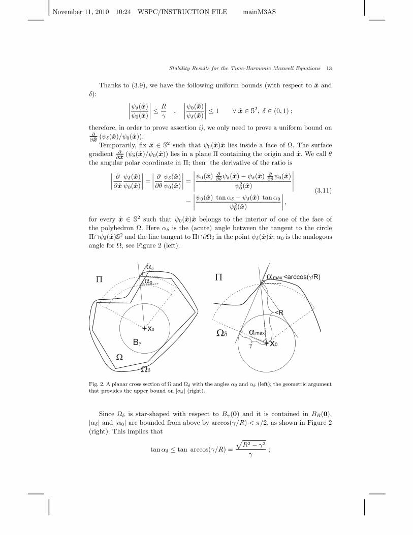
angle for Ω, see Figure 2 (left).

?

?d

Bg

x0

a

a

d

0P

?d

g x0

amaxP

amax

<R

<arccos( /R)g

Fig. 2. A planar cross section of Ω and Ωδ with the angles α0 and αδ (left); the geometric argumentthat provides the upper bound on |αδ| (right).

Since Ωδ is star-shaped with respect to Bγ(0) and it is contained in BR(0),

|αδ| and |α0| are bounded from above by arccos(γ/R) < π/2, as shown in Figure 2

(right). This implies that

tanαδ ≤ tan arccos(γ/R) =

√R2 − γ2

γ;



the same holds for α0. This in turns implies that the angular gradient of

ψδ(x)/ψ0(x) is uniformly bounded, with respect to δ and x, for almost every x

(only the points corresponding to edges and vertices of Ω are excluded, because the

gradient is not defined there). Finally, using the expression (3.10) of the Jacobians

proves assertion i).

Let us consider y ∈ ∂Ω such that it belongs to the interior of one of the faces

of Ω. Thanks to [2, Theorem 4.12], the harmonic function z defined in Lemma 3.3

can be extended in a neighborhood of y to a harmonic function z′. This implies

that z′ is C∞ in a neighborhood of y.

Identifying Ω with Ω0, we notice that

∂Ωδ = x ∈ BR(0) \ Ω : z′(x) = δ = ψδ(x)x, x ∈ S2 δ ∈ [0, δ∗).

Thanks to the smoothness of z′, we can apply the implicit function theorem (in

polar coordinates) and prove that the function

Ψ : S2 × [0, δ∗) → R

(x, δ) 7→ ψδ(x)

is smooth in a neighborhood of (y, 0). This implies the convergence

∂

∂yψδ(y)

δ→0−−−→ ∂

∂yψ0(y) for a.e. y ∈ S

2.

We see from (3.10) and (3.11) that assertion ii) follows from this result and from

the uniform convergence in S2 of ψδ to ψ0.

We can now prove the main result of this section.

Theorem 3.2. Let Ω ⊂ R3 be a bounded polyhedral domain which is star-shaped

with respect to Bγ(x0). Under the assumptions made on J , g and on the material

coefficients in Section 2, the result of Theorem 3.1 holds true.

Proof. Inspired by the proof of [10, Thm. 3.2.1.3], we harness the δ-uniform sta-

bility result of Theorem 3.1 for the smooth domains Ωδ introduced in Lemma 3.3.

Temporarily, fix δ ∈ (0, 1). First we map the data J and g in (2.1) to Ωδ by

suitable pullbacks w.r.t. Φ−1δ : for almost all x := Φδ(x) ∈ Ωδ we define

Jδ(x) := (detDΦ(x))−1DΦ(x)J(x) ,

gδ(x) := DΦ(x)−T g(x) .

Note that this ensures ∇ · Jδ = 0, if J is divergence freea. In addition, gδ will

be a tangential vector field on ∂Ωδ, provided that g is tangential to ∂Ω, see the

aThe operator e∇ indicates differentiation w.r.t. ex ∈ Ωδ.



discussion of pullbacks in [12, Sect. 2.2]. From the defining formulas and Lemma 3.4,

we immediately infer that, for all 0 < δ < δ0,

C−1 ‖J‖0,Ω ≤ ‖Jδ‖0,Ωδ≤ C ‖J‖0,Ω ,

C−1 ‖g‖0,∂Ω ≤ ‖gδ‖0,∂Ωδ≤ C ‖g‖0,∂Ω .

(3.12)

Next, we introduce Eδ ∈ Himp(curl; Ωδ) as solution of the variational problem

Aδ(Eδ, ξ) =

∫

Ωδ

Jδ · ξ dV +

∫

∂Ωδ

gδ · ξT dS ∀ ξ ∈ Himp(curl; Ωδ) , (3.13)

where the bilinear form Aδ(·, ·) is the counterpart of A(·, ·) from (2.3) in the do-

main Ωδ. Theorem 2.1 guarantees existence and uniqueness of Eδ. Further, from

Theorem 3.1, together with (3.12), we conclude the δ-uniform bound

∥∥∥µ−1/2∇ × Eδ

∥∥∥0,Ωδ

+ ω∥∥∥ε1/2Eδ

∥∥∥0,Ωδ

+∥∥∥λ1/2Eδ,T

∥∥∥0,∂Ωδ

≤ C(‖J‖0,Ω + ‖g‖0,∂Ω) , (3.14)

with a constant C > 0 depending only on the coefficients ε, µ, λ and the geometry

parameters γ and diam(Ω). Note that the δ-uniform bound on C is a consequence

of the information on the shape of the Ωδ’s gleaned from Lemma 3.3.

We pull Eδ back to Ω

Eδ(x) := DΦTδ (x)Eδ(x) , a.e. x ∈ Ω , (3.15)

with the special property [12, (2.15)]

(∇× Eδ)(x) = detDΦδ(x)DΦδ(x)−1(∇ × Eδ)(x) , x ∈ Ω . (3.16)

We easily find Eδ ∈ Himp(curl; Ω), since, thanks to Lemma 3.4,

C−1∥∥∥Eδ

∥∥∥0,Ω

≤ ‖Eδ‖0,Ωδ≤ C

∥∥∥Eδ

∥∥∥0,Ω

C−1∥∥∥∇× Eδ

∥∥∥0,Ω

≤∥∥∥∇ × Eδ

∥∥∥0,Ωδ

≤ C∥∥∥∇× Eδ

∥∥∥0,Ω

,

C−1∥∥∥Eδ,T

∥∥∥0,∂Ω

≤ ‖Eδ‖0,∂Ωδ≤ C

∥∥∥Eδ

∥∥∥0,∂Ω

,

for all 0 < δ < δ0. We can even conclude a counterpart of (3.14)

∥∥∥µ−1/2∇× Eδ

∥∥∥0,Ω

+ ω∥∥∥ε1/2Eδ

∥∥∥0,Ω

+∥∥∥λ1/2Eδ,T

∥∥∥0,∂Ω

≤ C(‖J‖0,Ω + ‖g‖0,∂Ω) . (3.17)

Using (3.15) and (3.16) we can transform the variational equation (3.13) to Ω and

find

Aδ(Eδ, ξ) :=

∫

Ω

µ−1Aδ(x)(∇× Eδ)(x) · (∇× ξ)(x)



− ω2εBδ(x)Eδ(x) · ξ(x) dV (x) − iω

∫

∂Ω

λCδ(x)Eδ,T (x) · ξT (x) dS(x)

= Aδ(Eδ, ξ)(3.13)=

∫

Ω

J(x) · ξ(x) dV (x) +

∫

∂Ω

Cδ(x)gT (x) · ξT (x) dS(x) , (3.18)

with matrix-valued functions on Ω and ∂Ω, respectively,

Aδ(x) := (detDΦδ(x))−1DΦδ(x)TDΦδ(x) for almost all x ∈ Ω ,

Bδ(x) := detDΦδ(x)DΦδ(x)−1DΦδ(x)−T for almost all x ∈ Ω ,

Cδ(x) := DΦδ(x)−1DΦδ(x)−TGδ(x) for almost all x ∈ ∂Ω ,

where Gδ ∈ L∞(∂Ω) is the Gram determinant (t1, t2 is any orthonormal basis of

the tangent space to ∂Ω at x)

Gδ(x) = |DΦδt1 ×DΦδ(x)t2| , x ∈ ∂Ω .

We remark that, thanks to Lemma 3.4, part ii), the matrix functions Aδ, Bδ and Cδ

are L2–convergent to the 3× 3 identity matrix Id3, for δ → 0. Eventually, in (3.18)

the test function ξ is obtained from ξ ∈ Himp(curl; Ωδ) by the transformation (3.15).

However, since the transformationHimp(curl; Ωδ) → Himp(curl; Ω), ξ 7→ ξ := DΦTδ ξ

is an isomorphism, (3.18) holds for any ξ ∈ Himp(curl; Ω) in place of ξ.

Owing to (3.17), we can find a sequence (δn)n∈N⊂ (0, δ0), δn → 0 for n → ∞,

and a vector field E∗ ∈ Himp(curl; Ω), such that, with En := Eδn ,

Enn→∞ E∗ weakly in Himp(curl; Ω) .

Observe that the weak limit E∗ also complies with the bound (3.17). To finish the

proof, we have to show that E∗ is the unique solution of the Maxwell variational

problem (2.3).

The sequences (Aδn)n∈N, (Bδn)n∈N

, (Cδn)n∈Nconverge to Id3, for n → ∞, in

L2 and almost everywhere in the respective domains; moreover, due to Lemma 3.4,

part i), they are also uniformly bounded with respect to δn. Since ξ ∈ Himp(curl; Ω),

by the dominated convergence theorem, we have

ATδn∇× ξ

n→∞−→ ∇× ξ ,

BTδn

ξn→∞−→ ξ ,

CTδn

ξTn→∞−→ ξT ,

strongly in the sense of L2. Consequently, since (En)n is weakly convergent in



Himp(curl; Ω), the weak versus strong convergence gives, for instance,

∫

Ω

µ−1Aδn(x)(∇× En)(x) · (∇× ξ)(x) dV (x)

=

∫

Ω

[µ−1(∇× En)(x)]︸︷︷︸weak

· [Aδn(x)T (∇× ξ)(x)]︸︷︷︸strong

dV (x)

n→∞−→∫

Ω

µ−1(∇× E∗)(x) · (∇× ξ)(x) dV (x) ;

the other integrals in the definition of Aδn(En, ξ) (see (3.18)) are amenable to

similar arguments, and, thus, we conclude

limn→∞

Aδn(En, ξ) = A(E∗, ξ) ∀ ξ ∈ Himp(curl; Ω) .

Therefore,

A(E∗, ξ)(3.18)= lim

n→∞

∫

Ω

J(x) · ξ(x) dV (x) +

∫

∂Ω

Cδn(x)gT (x) · ξT (x) dS(x)

=

∫

Ω

J(x) · ξ(x) dV (x) +

∫

∂Ω

gT (x) · ξT (x) dS(x) ,

(3.19)

by the dominated convergence theorem, because limδ→0 Cδ(x) = Id3 a.e. on ∂Ω, and

‖Cδ‖L∞(∂Ω)3×3 is δ-uniformly bounded. From (3.19) and (3.17) we finally conclude

the desired result.

4. Regularity of solutions in polyhedral domains

In this section, we establish the regularity of the solutions to problem (2.3) for

polyhedral domains, when g possesses extra smoothness.

The definition of Sobolev spaces on the polyhedral boundary requires care. De-

noting by Γj , j = 1, . . . ,m, the flat faces of ∂Ω, following [4, Section 2.3] we set

Hs(∂Ω) :=

ϕ ∈ H1(∂Ω) : ϕ|Γj

∈ Hs(Γj), j = 1, . . . ,m

if s ≥ 1 ,

ϕ ∈ L2(∂Ω) : ϕ = Φ|∂Ω for some Φ ∈ Hs+1/2(Ω)

if |s| < 1 ,

(4.1)

and

HsT (∂Ω) :=

ϕ ∈ L2

T (∂Ω) : ϕ|Γj∈ Hs(Γj)

2, j = 1, . . . ,m

∀ s ≥ 0 ;



notice that in [3, 4] the space HsT (∂Ω) was denoted Hs

−(∂Ω). The spaces Hs(∂Ω)

are endowed with the norms

‖ϕ‖s,∂Ω =

(‖ϕ‖2

1,∂Ω +∑m

j=1 ‖ϕ‖2s,Γj

)1/2

if s ≥ 1 ,

infΦ∈Hs+1/2(Ω): Φ|∂Ω=ϕ

‖Φ‖s+1/2,Ω if |s| < 1 .

Thanks to Corollary 1.4.4.5 of [10] and the standard Sobolev trace theorem (see

for instance [19, Thm. 3.9]), for 0 < s < 1/2 the spaces Hs(∂Ω) can be defined

piecewise, i.e.,

Hs(∂Ω) = ϕ ∈ L2(∂Ω) : ϕ|Γj∈ Hs(Γj), j = 1, . . . ,m, 0 < s < 1/2, (4.2)

with an equivalence between the two intrinsic norms; therefore we can identify the

spaces

HsT (∂Ω) = Hs(∂Ω)3 ∩ L2

T (∂Ω), 0 < s < 1/2. (4.3)

From [3, Thm. 3.9 and Thm. 3.10] (see also [5, Thm. 4.1]), we learn that, if

U ∈ H(curl,Ω), then

divT (U × n) ∈ H−1/2(∂Ω), curlT (UT ) ∈ H−1/2(∂Ω) ,

‖divT (U × n)‖−1/2,∂Ω ≤ C(‖U‖0,Ω + ‖∇ × U‖0,Ω

),

‖curlT (UT )‖−1/2,∂Ω ≤ C(‖U‖0,Ω + ‖∇ × U‖0,Ω

),

(4.4)

where curlT and divT are the surface curl and the surface divergence on ∂Ω, respec-

tively, and the constant C > 0 is independent of U .

The identifications (4.3) and (4.2) imply the continuity of the surface differential

operators:

divT , curlT : HsT (∂Ω) → Hs−1(∂Ω) , 0 < s < 1/2 . (4.5)

Eventually, the standard trace theorem for Sobolev spaces yields the continuity

of the tangential traces (see [3, p. 11])H1(Ω)3 → H

1/2T (∂Ω)

U 7→ UT,

H1(Ω)3 → H

1/2T (∂Ω)

U 7→ U × n. (4.6)

The following lemma provides a simple regularity result for the Laplace equation

in the context of the spaces defined in (4.1). As a by-product, we obtain embeddings

between the Sobolev spaces on ∂Ω defined piecewise as above and the ones defined

as traces of functions in Ω, as in [19]; see Remark 4.2 below.

Lemma 4.1. Let Ω be a Lipschitz polyhedron. Then there exists sΩ depending only

on Ω, 0 < sΩ < 1/2, such that if ϕ satisfies−∆ϕ = 0 on Ω,

ϕ|∂Ω ∈ Hs(∂Ω),



for some 1 < s ≤ 1 + sΩ, then ϕ belongs to Hs+1/2(Ω). Moreover the following

bound holds

‖ϕ‖s+1/2,Ω ≤ C ‖ϕ‖s,∂Ω . (4.7)

Proof. We know from the definition (4.1) that the trace operator from Ht(Ω) to

Ht−1/2(∂Ω) is continuous and surjective for any 1/2 < t < 1. This, together with

(4.3), implies that Proposition 3.7 in [1] (see also [19, Thm. 3.50]) can be slightly

generalized as follows: given

v ∈ H(curl; Ω) ∩H(div; Ω) such that vT ∈ Ht−1/2T (∂Ω), 1/2 < t < 1, (4.8)

then v ∈ Hmin1/2+sΩ,t(Ω) for some positive sΩ depending only on Ω. Also the

bound in [19, Thm. 3.50] can be generalized as

‖v‖t,Ω ≤ C(‖v‖0,Ω + ‖∇× v‖0,Ω + ‖∇ · v‖0,Ω + ‖v‖t−1/2,∂Ω

), (4.9)

for every 1/2 < t ≤ 1/2 + sΩ < 1.

We define the vector field w = ∇ϕ, it satisfies the condition (4.8) since

∇ × w = 0, ∇ · w = 0 and its tangential trace is wT = ∇Tϕ ∈ Hs−1(∂Ω)3 ∩L2(∂Ω) = Hs−1

T (∂Ω) thanks to (4.3); therefore w belongs to Hs−1/2(Ω) and finally

ϕ ∈ Hs+1/2(Ω).

The bound (4.7) follows from

‖ϕ‖s+1/2,Ω ≤ C(‖ϕ‖0,Ω + ‖w‖s−1/2,Ω)

(4.9)

≤ C(‖ϕ‖0,Ω + ‖w‖0,Ω + ‖∇Tϕ‖s−1,∂Ω)

(4.2)

≤ C(‖ϕ‖1/2,∂Ω +

m∑

j=1

‖∇Tϕ‖s−1,Γj)

≤ C ‖ϕ‖s,∂Ω ,

where we have used the usual H1–stability of the Laplace problem for u, see for

instance [19, Thm. 3.12].

Remark 4.1. From the proof of the previous lemma, it is clear that the parameter

sΩ is equal to the one called s in [1, Prop. 3.7].

Whenever the domain is convex, Theorem 2.17 of [1] applies and Lemma 4.1

holds for every 1 < s < 3/2.

Remark 4.2. Lemma 4.1 provides the embedding

Hs(∂Ω) ⊆ϕ ∈ L2(∂Ω) : ϕ = Φ|∂Ω for some Φ ∈ Hs+1/2(Ω)

,

for 1 < s < 1 + sΩ; moreover the immersion is continuous, i.e.,

infΦ∈Hs+1/2(Ω), Φ|∂Ω=ϕ

‖Φ‖s+1/2,Ω ≤ C ‖ϕ‖s,∂Ω . (4.10)



The opposite inclusion

Hs(∂Ω) ⊇ϕ ∈ L2(∂Ω) : ϕ = Φ|∂Ω for some Φ ∈ Hs+1/2(Ω)

holds in the larger range 1 < s < 3/2 and it is a simple consequence of the definition

(4.1): for every Φ ∈ Hs+1/2(Ω), 1 < s < 3/2,

‖Φ‖s,∂Ω ≤ C(‖Φ‖0,∂Ω + ‖∇Φ‖0,∂Ω +

m∑

j=1

‖∇Φ‖s−1,Γj

)

(4.2)

≤ C(‖Φ‖0,∂Ω + ‖∇Φ‖s−1,∂Ω

)

≤ C ‖Φ‖s+1/2,Ω .

Notice that in the limit case s = 3/2, (4.10) does not hold: Theorem 3.4 of [3] shows

that the traces of functions in H2(Ω) can not be defined piecewise on the faces of

a polyhedron, but tangential continuity is required along the edges.

Remark 4.3. Lemma (4.1) implies Theorem 3.18 of [19]. Notice that the definition

of Hs(∂Ω) for s > 1 given in [19, (3.12)] is different from the one used in this paper.

A last elliptic regularity result will be instrumental in the treatment of Maxwell

solutions: it concerns the Laplace-Beltrami operator ∆T = divT ∇T , where ∇T

denotes the tangential gradient, and is stated in [4, Thm. 8]; we report it here, for

the sake of completeness.

Lemma 4.2. For any bounded Lipschitz polyhedral domain, there is a 0 < s∗ ≤ 1

depending only on the shape of ∂Ω in neighborhoods of vertices, such that

∆Tψ ∈ H−1+s(∂Ω) for some s > 0

⇒ ψ ∈ H1+sLB (∂Ω) ∀ 0 < sLB ≤ s, sLB < s∗ .

The case sLB = s, when s < s∗, can be deduced from the proof of [4, Thm. 8].

Moreover, formula (57) in [4] shows that, whenever Ω is convex, it is possible to

choose s∗ = 1.

We are now ready to prove the main theorem of this section, namely, a regularity

result for the solutions of the Maxwell equations.

Theorem 4.4. Let Ω ⊂ R3 be a bounded polyhedral domain which is star-shaped

with respect to Bγ(x0). In addition to the assumptions made on J , g and on the

material coefficients in Section 2, we assume g ∈ Hsg

T (∂Ω), with 0 < sg < 1/2.

Then the solution E to problem (2.3) satisfies

E ∈ H1/2+s(Ω)3 and ∇× E ∈ H1/2+s(Ω)3

for all the real parameters s such that

0 < s ≤ minsg, sΩ and s < s∗ ,

where sΩ is defined in Lemma 4.1 (or in [1, Prop. 3.7]), and s∗ is defined in

Lemma 4.2 (or in [4, Thm. 8]).



Moreover, we have the following stability estimate: there is a positive constant

C independent of ω, but depending on s, Ω, γ, λ, ǫ and µ, such that

‖∇× E‖1/2+s,Ω + ω ‖E‖1/2+s,Ω ≤ C((1 + ω)(‖J‖0,Ω + ‖g‖0,∂Ω) + ‖g‖sg,∂Ω

).

(4.11)

Proof. In this proof, we denote by C a positive constant independent of ω, but

depending on λ, Ω, ǫ and µ, whose value might change at each occurrence.

We start by by proving the regularity of E, following the reasoning of [8,

Sect. 4.5.d].

Decompose E as

E = ΦΦΦ0 + ∇ψ ,where ΦΦΦ0 ∈ H1(Ω)3 ∩H(div0; Ω), ψ ∈ H1(Ω) and

∥∥ΦΦΦ0∥∥

1,Ω+ ‖ψ‖1,Ω ≤ C (‖E‖0,Ω + ‖∇ × E‖0,Ω) (4.12)

(see [12, Lemma 2.4]); clearly, ∆ψ = 0 in Ω.

By using this decomposition, we can write the boundary condition in prob-

lem (2.2) by

(µ−1∇× E) × n − iωλΦΦΦ0T − iωλ∇Tψ = g on ∂Ω , (4.13)

where ∇Tψ is the tangential gradient of ψ on ∂Ω, i.e., ∇Tψ := (n ×∇ψ) × n.

Using (4.4), the tangential divergence divT of (µ−1∇× E) × n is well-defined,

belongs to H−1/2(∂Ω) and∥∥divT

((µ−1∇× E) × n

)∥∥−1/2,∂Ω

≤ C(∥∥µ−1∇× E

∥∥0,Ω

+∥∥∇× (µ−1∇× E)

∥∥0,Ω

).

(4.14)

Since g ∈ Hsg

T (∂Ω), (4.5) gives divT g ∈ Hsg−1(∂Ω). Moreover, (4.6) and (4.5) imply

divT ΦΦΦ0T ∈ H−1/2−η(∂Ω) for all η ∈ (0, 1/2], in particular, divT ΦΦΦ0

T ∈ Hsg−1(∂Ω);

they also imply the bounds∥∥divT ΦΦΦ0

T

∥∥sg−1,∂Ω

≤ C∥∥ΦΦΦ0

T

∥∥sg−1,∂Ω

≤ C∥∥ΦΦΦ0

∥∥1,∂Ω

.

From the regularities of the tangential divergence of the terms in (4.13), it follows

that

divT λ∇Tψ ∈ Hsg−1(∂Ω).

Due to the smoothness of the solutions to the Laplace-Beltrami equation provided

by Lemma 4.2, we have that ψ ∈ H1+sLB (∂Ω), for every 0 < sLB ≤ sg, sLB < s∗,

where s∗ is defined in Lemma 4.2. Lemma 4.1 ensures that ψ ∈ H3/2+s(Ω), for

every 0 < s ≤ minsg, sΩ, s < s∗, where 0 < sΩ < 1/2 is given in Lemma 4.1b.

bWhenever Ω is convex, the parameter L in [4, Thm. 8] is equal to 2π, thus s∗ = 1. Moreover,thanks to Remark 4.1, sΩ can be chosen equal to sg. Therefore, if Ω is convex, the only conditionon s is 0 < s ≤ sg.



Moreover the previous steps give

‖ψ‖3/2+s,Ω

(4.7)

≤ C ‖ψ‖1+s,∂Ω

[15, eq. (2.2)]

≤ C ‖divT λ∇Tψ‖sg−1,∂Ω . (4.15)

From ΦΦΦ0 ∈ H1(Ω)3 and ∇ψ ∈ H1/2+s(Ω)3, we have that E ∈ H1/2+s(Ω)3.

We proceed by bounding ‖E‖1/2+s,Ω. By the triangle inequality, we have

‖E‖1/2+s,Ω ≤∥∥ΦΦΦ0

∥∥1/2+s,Ω

+ ‖∇ψ‖1/2+s,Ω ,

and we bound the two terms on the right-hand side separately.

From (4.12) and Theorem 3.2 (see (3.1)), we obtain∥∥ΦΦΦ0

∥∥1,Ω

≤ C (1 + ω−1) (C1 ‖J‖0,Ω + C2 ‖g‖0,∂Ω) . (4.16)

Collecting the bounds proved so far, we obtain

‖∇ψ‖1/2+s,Ω

(4.15)

≤ C ‖divT λ∇Tψ‖sg−1,∂Ω

(4.13)

≤ C(ω−1

∥∥divT

((µ−1∇× E) × n

)∥∥sg−1,∂Ω

+∥∥divT λΦΦΦ

0T

∥∥sg−1,∂Ω

+ ω−1 ‖divT g‖sg−1,∂Ω

)

(4.5)

≤ C(ω−1

∥∥divT

((µ−1∇× E) × n

)∥∥−1/2,∂Ω

+∥∥ΦΦΦ0

T

∥∥sg,∂Ω

+ ω−1 ‖g‖sg,∂Ω

)

(4.14), (4.6)

≤ C(ω−1 ‖∇ × E‖0,Ω + ω−1 ‖∇ ×∇× E‖0,Ω

+∥∥ΦΦΦ0

∥∥1,Ω

+ ω−1 ‖g‖sg ,∂Ω

)

(2.2), (4.16)

≤ C(ω−1 ‖∇× E‖0,Ω + ω ‖E‖0,Ω + ω−1 ‖J‖0,Ω

+ (1 + ω−1) (C1 ‖J‖0,Ω + C2 ‖g‖0,∂Ω) + ω−1 ‖g‖sg,∂Ω

)

(3.1), Thm. 3.2

≤ C((C1 + ω−1C1 + ω−1) ‖J‖0,Ω

+ (1 + ω−1)C2 ‖g‖0,∂Ω + ω−1 ‖g‖sg,∂Ω

).

Therefore, we have the bound

ω ‖E‖1/2+s,Ω ≤ C((1+C1 +C1ω) ‖J‖0,Ω +(1+ω)C2 ‖g‖0,∂Ω +‖g‖sg,∂Ω

). (4.17)

Similarly, we prove the smoothness of ∇× E. Decompose ∇× E as

∇× E = ΨΨΨ0 + ∇φ ,where ΨΨΨ0 ∈ H1(Ω)3 ∩H(div0; Ω), and φ ∈ H1(Ω); again, ∆φ = 0 in Ω and

∥∥ΨΨΨ0∥∥

1,Ω+ ‖φ‖1,Ω ≤ C

(‖∇× E‖0,Ω + ‖∇ ×∇× E‖0,Ω

)

≤ C(‖∇× E‖0,Ω + ω2 ‖E‖0,Ω + ‖J‖0,Ω

),

(4.18)



where the second inequality follows from the first equation in (2.2). The boundary

condition in problem (2.2) can be written as

µ−1ΨΨΨ0 × n + µ−1∇φ× n − iωλET = g on ∂Ω . (4.19)

Thanks to (4.4), the tangential curl curlT of λET is well-defined, belongs to

H−1/2(∂Ω) and

‖curlT λET ‖−1/2,∂Ω ≤ C (‖E‖0,Ω + ‖∇× E‖0,Ω) . (4.20)

Since g ∈ Hsg

T (∂Ω)3, (4.5) gives curlT g ∈ Hsg−1(∂Ω). Moreover, ΨΨΨ0 × n ∈H

1/2T (∂Ω)3 by (4.6), then curlT (µ−1ΨΨΨ0×n) ∈ H−1/2−η(∂Ω), for every 0 < η < 1/2,

by (4.5), in particular, curlT (µ−1ΨΨΨ0 × n) ∈ Hsg−1(∂Ω). Thus, since

curlT (µ−1∇φ× n) = − divT

(n × (µ−1∇φ× n)

)= − divT µ

−1∇Tφ

(see [18, Formula (3.15), p. 49]), we have that

divT µ−1∇Tφ ∈ Hsg−1(∂Ω) .

Proceeding exactly as we did to prove (4.15), Lemmas 4.1 and 4.2 ensure that the

harmonic function φ belongs to H3/2+s(Ω) with the parameter s in the same range

as before (0 < s ≤ minsg, sΩ, s < s∗), and

‖φ‖3/2+s,Ω

(4.7)

≤ C ‖φ‖1+s,∂Ω

[15, eq. (2.2)]

≤ C ‖divT λ∇Tφ‖sg−1,∂Ω . (4.21)

From Ψ0 ∈ H1(Ω)3 and ∇φ ∈ H1/2+s(Ω)3, we have that ∇× E ∈ H1/2+s(Ω)3.

For the bound of ‖∇× E‖1/2+s,Ω, the triangle inequality gives

‖∇× E‖1/2+s,Ω ≤∥∥ΨΨΨ0

∥∥1/2+s,Ω

+ ‖∇φ‖1/2+s,Ω .

Again as in the first part of this proof, from (4.18) and Theorem 3.2 (see (3.1)), we

have∥∥ΨΨΨ0

∥∥1,Ω

≤ C((1 + C1 + C1ω) ‖J‖0,Ω + (1 + ω)C2 ‖g‖0,∂Ω

).

For ‖∇φ‖1/2+s,Ω, by proceeding as in the first part of this proof, using (4.21),

the boundary condition (4.19), the bound (4.20), the continuity (4.5), the stability

bound (4.18) and Theorem 3.2 (see (3.1)) we have

‖∇φ‖1/2+s,Ω ≤ C((1 + C1 + C1ω) ‖J‖0,Ω + (1 + ω)C2 ‖g‖0,∂Ω + ‖g‖sg,∂Ω

)

and consequently

‖∇ × E‖1/2+s,Ω ≤ C((1 + C1 + C1ω) ‖J‖0,Ω + (1 + ω)C2 ‖g‖0,∂Ω + ‖g‖sg,∂Ω

).

(4.22)

The bounds (4.17) and (4.22) give the stability bound (4.11).

Remark 4.5. In the case of convex polyhedral domains, the smoothness parame-

ters s reaches the regularity of the boundary datum s = sg < 1/2, since Lemma 4.1

holds true for all 0 < sΩ < 1/2, and s∗ = 1 in Lemma 4.2 (see footnote 2).



Remark 4.6. The regularity of solutions stated in Theorem 4.4 guarantees that

the tangential traces of E and ∇× E are in L2T (∂Ω).

Remark 4.7. For C2–domains, under all the other assumptions made in Theo-

rem 4.4, the H1–regularity of both E and ∇ × E was already established in [8,

Sect. 4.5.d] (see also Lemma 3.2 in this paper); the stability estimate

‖∇ × E‖1,Ω + ω ‖E‖1,Ω ≤ C((1 + ω)(‖J‖0,Ω + ‖g‖0,∂Ω) + ‖g‖1/2,∂Ω

)

can be obtained along the lines of the proof of Theorem 4.4.

5. Conclusion

In this paper, we have established some new regularity results and stability estimates

for solutions to the time-harmonic Maxwell equations with impedance boundary

conditions. More precisely, we have proved stability estimates with constant inde-

pendent of the wavenumber for smooth domains and for polyhedral domains (see

Theorem 3.1 and Theorem 3.2, respectively), and an elliptic regularity result for

polyhedral domains (see Theorem 4.4).

Possible applications of these results are the convergence analysis of numerical

methods for the approximation of Maxwell’s equations and the stability analysis of

electromagnetic boundary integral operators. For these applications, some extension

of Theorem 3.1 (stability for smooth domains) might be interesting: i) to non-star

shaped domains; in this case, in the definition of the test function ξ, x should be

substituted by a more general vector field; ii) to domains containing a (star-shaped)

hole and with mixed boundary conditions, in order to extend to the Maxwell case

the results proved in [11] for the Helmholtz problem; this would be the key point

to extend to this case also all the other results proved for polyhedral domains; iii)

to non-constant or anisotropic material coefficients ǫ and µ; the key tool for this

extension would be the use of more general Rellich identities, as the one introduced

by Payne and Weinberger in [21] (see also [20, Sect. 5.1.1] and [16, Lemma 4.22]).

Acknowledgment

This section should come after the Appendices if any and should be unnumbered.

Funding information may also be included here.

References

References

1. C. Amrouche, C. Bernardi, M. Dauge, and V. Girault, Vector potentials in

three-dimensional non-smooth domains, Math. Methods Appl. Sci., 21 (1998), pp. 823–864.

2. S. Axler, P. Bourdon, and W. Ramey, Harmonic function theory, Graduate Textsin Mathematics, Springer-Verlag, New York, 2001.



3. A. Buffa and P. Ciarlet, Jr., On traces for functional spaces related to Maxwell’s

equations. I. An integration by parts formula in Lipschitz polyhedra, Math. MethodsAppl. Sci., 24 (2001), pp. 9–30.

4. A. Buffa, M. Costabel, and C. Schwab, Boundary element methods for Maxwell’s

equations on non-smooth domains, Numer. Math., 92 (2002), pp. 679–710.5. A. Buffa, M. Costabel, and D. Sheen, On traces for H(curl, Ω) in Lipschitz

domains, J. Math. Anal. Appl., 276 (2002), pp. 845–867.6. S. N. Chandler-Wilde and P. Monk, Wave-number-explicit bounds in time-

harmonic scattering, SIAM J. Math. Anal., 39 (2008), pp. 1428–1455.7. P. Cummings and X. Feng, Sharp regularity coefficient estimates for complex-valued

acoustic and elastic Helmholtz equations, Math. Models Methods Appl. Sci., 16 (2006),pp. 139–160.

8. M. Dauge, M. Costabel, and S. Nicaise, Corner Singularities and Analytic Reg-

ularity for Linear Elliptic Systems. Part I:

Smooth domains, Tech. Rep. 10-09, IRMAR, 2010. Available at http://perso.univ-rennes1.fr/monique.dauge/publis/CoDaNi Analytic Part I.pdf.

9. V. Girault and P.-A. Raviart, Finite element methods for Navier-Stokes equations,vol. 5 of Springer Series in Computational Mathematics, Springer-Verlag, Berlin, 1986.Theory and algorithms.

10. P. Grisvard, Elliptic problems in nonsmooth domains, vol. 24 of Monographs andStudies in Mathematics, Pitman (Advanced Publishing Program), Boston, MA, 1985.

11. U. Hetmaniuk, Stability estimates for a class of Helmholtz problems, Communicationsin Mathematical Sciences, 5 (2007), pp. 665–678.

12. R. Hiptmair, Finite elements in computational electromagnetism, Acta Numer., 11(2002), pp. 237–339.

13. R. Hiptmair, A. Moiola, and I. Perugia, The Trefftz-DG method for the time-

harmonic Maxwell equations. In preparation.14. , Plane wave discontinuous Galerkin methods for the 2D Helmholtz equation:

analysis of the p–version, Tech. Rep. 2009-20, SAM-ETH Zurich, 2009.15. R. Hiptmair and C. Schwab, Natural boundary element methods for the electric

field integral equation on polyhedra, SIAM J. Numer. Anal., 40 (2002), pp. 66–86.16. W. McLean, Strongly elliptic systems and boundary integral equations, Cambridge

University Press, Cambridge, 2000.17. J. Melenk, On Generalized Finite Element Methods, PhD thesis, University of Mary-

land, USA, 1995.18. P. Monk, Finite element methods for Maxwell’s equations, Clarendon Press, Oxford,

2003.19. P. Monk, Finite element methods for Maxwell’s equations, Numerical Mathematics

and Scientific Computation, Oxford University Press, New York, 2003.20. J. Necas, Les methodes directes en theorie des equations elliptiques, Masson et Cie,

Editeurs, Paris, 1967.21. L. E. Payne and H. F. Weinberger, New bounds for solutions of second order

elliptic partial differential equations, Pacific J. Math., 8 (1958), pp. 551–573.22. J.-P. Rosay and W. Rudin, A maximum principle for sums of subharmonic func-

tions, and the convexity of level sets, Michigan Math. J., 36 (1989), pp. 95–111.23. E. A. Spence, S. N. Chandler-Wilde, I. G. Graham, and V. P. Smyshlyaev,

A new frequency-uniform coercive boundary integral equation for acoustic scattering.Report. Department of Mathematics, University of Bath. Submitted, 2010.

stability results for the time-harmonic maxwell equations

Documents