Michael Armstrong, Christine Ross, Danny Phillips, and Mark BlackwelderRolls-Royce North American Technologies, Inc.—LibertyWorks, Indianapolis, Indiana

Stability, Transient Response, Control, and Safety of a High-Power Electric Grid for Turboelectric Propulsion of Aircraft

NASA/CR—2013-217865

June 2013

https://ntrs.nasa.gov/search.jsp?R=20140000336 2018-05-28T17:54:35+00:00Z

NASA STI Program . . . in Profi le

Since its founding, NASA has been dedicated to the advancement of aeronautics and space science. The NASA Scientifi c and Technical Information (STI) program plays a key part in helping NASA maintain this important role.

The NASA STI Program operates under the auspices of the Agency Chief Information Offi cer. It collects, organizes, provides for archiving, and disseminates NASA’s STI. The NASA STI program provides access to the NASA Aeronautics and Space Database and its public interface, the NASA Technical Reports Server, thus providing one of the largest collections of aeronautical and space science STI in the world. Results are published in both non-NASA channels and by NASA in the NASA STI Report Series, which includes the following report types: • TECHNICAL PUBLICATION. Reports of

completed research or a major signifi cant phase of research that present the results of NASA programs and include extensive data or theoretical analysis. Includes compilations of signifi cant scientifi c and technical data and information deemed to be of continuing reference value. NASA counterpart of peer-reviewed formal professional papers but has less stringent limitations on manuscript length and extent of graphic presentations.

• TECHNICAL MEMORANDUM. Scientifi c

and technical fi ndings that are preliminary or of specialized interest, e.g., quick release reports, working papers, and bibliographies that contain minimal annotation. Does not contain extensive analysis.

• CONTRACTOR REPORT. Scientifi c and

technical fi ndings by NASA-sponsored contractors and grantees.

• CONFERENCE PUBLICATION. Collected papers from scientifi c and technical conferences, symposia, seminars, or other meetings sponsored or cosponsored by NASA.

• SPECIAL PUBLICATION. Scientifi c,

technical, or historical information from NASA programs, projects, and missions, often concerned with subjects having substantial public interest.

• TECHNICAL TRANSLATION. English-

language translations of foreign scientifi c and technical material pertinent to NASA’s mission.

Specialized services also include creating custom thesauri, building customized databases, organizing and publishing research results.

For more information about the NASA STI program, see the following:

• Access the NASA STI program home page at http://www.sti.nasa.gov

• E-mail your question to help@sti.nasa.gov • Fax your question to the NASA STI

Information Desk at 443–757–5803 • Phone the NASA STI Information Desk at 443–757–5802 • Write to:

STI Information Desk NASA Center for AeroSpace Information 7115 Standard Drive Hanover, MD 21076–1320

Michael Armstrong, Christine Ross, Danny Phillips, and Mark BlackwelderRolls-Royce North American Technologies, Inc.—LibertyWorks, Indianapolis, Indiana

Stability, Transient Response, Control, and Safety of a High-Power Electric Grid for Turboelectric Propulsion of Aircraft

NASA/CR—2013-217865

June 2013

National Aeronautics andSpace Administration

Glenn Research CenterCleveland, Ohio 44135

Prepared under Contract NNC10BA14B

Available from

NASA Center for Aerospace Information7115 Standard DriveHanover, MD 21076–1320

National Technical Information Service5301 Shawnee Road

Alexandria, VA 22312

Available electronically at http://www.sti.nasa.gov

Trade names and trademarks are used in this report for identifi cation only. Their usage does not constitute an offi cial endorsement, either expressed or implied, by the National Aeronautics and

Space Administration.

Level of Review: This material has been technically reviewed by NASA technical management.

Acknowledgments

Special thanks to Marty Bradley, John Fifi eld, and John Sheen from the Boeing Company for their contributions to this research effort.

NASA/CR—2013-217865 iii

Contents

Summary .................................................................................................................................... 1 1. Turboelectric Distributed Propulsion System Issues ................................................................ 4

1.1 System Level Performance/Stability/Safety Issues ......................................................... 4 1.1.1 System Level Dynamic Considerations .................................................................. 5 1.1.2 Implementation Considerations ............................................................................. 6

1.2 Nominal/Off-Nominal Operating Scenarios Issues .......................................................... 7 1.2.1 Exogenous Failure Conditions ............................................................................... 7 1.2.2 Endogenous Failure Conditions ............................................................................. 9

1.3 Architecture Design Decisions/Issues ............................................................................13 1.3.1 Bus Voltage Issues ...............................................................................................14 1.3.2 Physical Definition Design Issues .........................................................................14 1.3.3 Definition System/Component Roles ....................................................................14 1.3.4 Failure Response Strategies .................................................................................14

2. Issue Prioritization ................................................................................................................. 16 2.1 Issue Evaluation Categories ..........................................................................................16

2.1.1 Applicability to Electrical Grid Stability and Control ...............................................16 2.1.2 Probability of Occurrence and Severity of Potential Impact ...................................16 2.1.3 Triviality of the Solution .........................................................................................16 2.1.4 Programmatic Constraints ....................................................................................17

2.2 Issue Rankings ..............................................................................................................17 3. Architecture Trades ............................................................................................................... 21

3.1 Contingency Analysis ....................................................................................................21 3.1.1 Generators/Converters .........................................................................................23 3.1.2 Distribution ...........................................................................................................24 3.1.3 Propulsors ............................................................................................................25

3.2 System Level Architecture Concepts .............................................................................26 3.2.1 Concept 1: Baseline Architecture ..........................................................................27 3.2.2 Concept 2: Inner Bus Tie ......................................................................................28 3.2.3 Concept 3: 3-Bus Multi-Feeder Architecture .........................................................29 3.2.4 Concept 4: Cross-Redundant Multi-Feeder Architecture .......................................30

3.3 Architecture Component Breakdown .............................................................................31 4. Architecture Sizing Analysis .................................................................................................. 32

4.1 Component Power, Torque, and Current Densities .......................................................32 4.2 Architecture Weight Comparison ...................................................................................33

5. Component Technology Evaluation ....................................................................................... 37 5.1 Superconducting Generator/Motor ................................................................................37 5.2 Converter Technology ...................................................................................................38 5.3 HVDC Power Distribution ..............................................................................................39

5.3.1 Voltage Level ........................................................................................................39 5.3.2 DC Voltage Configuration .....................................................................................41

5.4 Protection ......................................................................................................................42 5.4.1 Protection Implementation ....................................................................................42 5.4.2 Strategies .............................................................................................................43 5.4.3 Detection ..............................................................................................................45 5.4.4 Protection Equipment ...........................................................................................46

6. Architecture Selection ........................................................................................................... 54 7. Model Overview .................................................................................................................... 56

7.1 Assumptions/Limitations ................................................................................................58 7.2 Model Elements.............................................................................................................62

NASA/CR—2013-217865 iv

7.2.1 Engine ..................................................................................................................62 7.2.2 Generator .............................................................................................................64 7.2.3 Buses and Energy Storage ...................................................................................65 7.2.4 Propulsors ............................................................................................................70

7.3 Simulation Setup ...........................................................................................................71 7.3.1 Scenario Requirements ........................................................................................71 7.3.2 System Attributes .................................................................................................71 7.3.3 Failure Insertion/Response ...................................................................................73

7.4 Simulation Outputs ........................................................................................................77 7.4.1 Nominal Operations: Command Response ...........................................................77 7.4.2 Off-Nominal Operations: Failure Recovery ...........................................................83

7.5 Modeling Section Review ..............................................................................................88 8. System Sensitivity Study ....................................................................................................... 89

8.1 Design of Experiments ..................................................................................................89 8.1.1 Thrust Response Scenario Neural Net Error Overview .........................................91 8.1.2 Engine Failure Scenario Neural Net Error Overview .............................................92

8.2 Sensitivity Analysis Results ...........................................................................................95 8.2.1 Step Change in Thrust ..........................................................................................95 8.2.2 Engine Failure ......................................................................................................97

8.3 Energy Storage Pareto Optimization .............................................................................98 9. Conclusions ........................................................................................................................ 104

9.1 Key Observations and Challenges .............................................................................. 104 9.1.1 Issue Identification and Selection........................................................................ 104 9.1.2 Architecture Selection and Sizing ....................................................................... 105 9.1.3 System Modeling and Factor Sensitivity ............................................................. 106

9.2 Future Work ................................................................................................................ 107 9.2.1 Vehicle Level Requirements Update ................................................................... 107 9.2.2 Directional Control Modeling and Trade Studies ................................................. 108 9.2.3 Architecture Modeling ......................................................................................... 108 9.2.4 Protection and Control Studies ........................................................................... 108 9.2.5 Wholly Cryogenic System Demonstrator ............................................................. 108

Appendix A. Candidate Architectures ...................................................................................... 111 Appendix B. Thrust Response Regression Equation ............................................................... 115 Appendix C. Thrust Recovery Regression Equations .............................................................. 119

NASA/CR—2013-217865 1

Summary This document contains the deliverables for the NASA Research and Technology for

Aerospace Propulsion Systems (RTAPS) regarding the stability, transient response, control, and safety study for a high power cryogenic turboelectric distributed propulsion (TeDP) system. The objective of this research effort is to enumerate, characterize, and evaluate the critical issues facing the development of the N3-X concept aircraft. This includes the proposal of electrical grid architecture concepts and an evaluation of any needs for energy storage.

NASA’s N3-X hybrid wing body aircraft concept promises dramatic improvements to aircraft performance pursuant to N+3 targets. A significant portion of these potential improvements are attributed to closely coupled integration of propulsion, power, and vehicle aerodynamic design. This integration is enabled by an advanced TeDP system1,2.

The current iteration of this vehicle’s TeDP architecture includes two turboshaft engines positioned at the wingtips and a slotted bank of propulsors positioned at the trailing edge of the lifting body3,4. The turboshaft engine drives the superconducting electrical machines used to generate power. This power is converted from alternating current (AC) to direct current (DC) and distributed to the centrally located propulsors.

Providing propulsive power in this fashion introduces three distinct benefits. First, DC power distribution allows for the decoupling of the fan and engine speeds. There is no need to match the speeds of the turbine engines or the propulsor fans. Each propulsor can be individually throttled to achieve the optimal pressure ratio. Additionally, higher propulsive efficiency is attained by operating at very large effective bypass ratios. Finally, reductions in fuel burn may also be achieved through boundary layer ingestion5.

While the advantages of this concept are attractive, significant design challenges arise from this dramatic shift in aircraft systems architecture. For this aircraft, the propulsion system is required to produce and distribute 30,000 horsepower (hp) at a minimum to provide thrust during takeoff. This requires that the generator or generators drawing power from each turboshaft engine be rated to a minimum of 22.4 MVA. For such a high power electric system, the losses from normal conducting electrical components would be significant. To achieve maximum efficiency of the electrical system, an entirely superconducting and cryogenic electrical system with DC distribution is proposed. In addition to eliminating AC losses, a DC distribution system eliminates the need to synchronize multiple AC generators to an AC distribution system and also decouples the fan and engine speeds. The additional weight and power requirements to cool the superconducting electrical system is not considered in this study, although NASA has studied these additional power requirements2,5.

In addition to being more efficient, superconducting electrical system components have higher power density (kW/kg), torque density (Nm/kg), or current density (A/m2/kg) compared to conventional normal conducting, room temperature components. These high density components enable the weight of the electric propulsion system to be minimized while meeting the high power demand.

This wholly superconducting electrical system must meet all steady-state and transient thrust requirements including potential differential yaw control for stability augmentation under the same reliability requirements as a traditional tube-and-wing concept with podded propulsion. Reliability and fail-safe requirements must be met at minimal weight penalty and acceptable levels of system complexity.

The research presented in this report focuses exclusively on the electrical power systems for this aircraft. All cryogenic support for the cold components is assumed to be sufficiently redundant and is not considered in the issue assessment, architecture definition, and system modeling. Additionally, detailed modeling of the superconducting machines and the cryogenic

NASA/CR—2013-217865 2

inverters is not considered to be a part of this Task. As will be discussed in this report, the models generated for system analysis are generic dynamic representations of component responses to power demands.

Although mass and performance models were not generated in association with this task, component and system weights were approximated to differentiate between candidate architecture concepts. The primary objectives of this study were to explore architecture solutions for providing vehicle propulsion power. Therefore, the nonpropulsive electrical system for the aircraft was neglected for the purposes of this study.

The project tasks delivered for this research effort are presented in three main parts of this document. The first part of this work is the identification and prioritization of TeDP electrical grid issues to be explored with system modeling and simulation. This effort is discussed in Sections 1 and 2 of this report. Section 1 reviews the fundamental issues that may be encountered in the design and operation of this system. In Section 2, the prioritization and selection schemes are described. Exogenous (source of disturbances external to system) and endogenous (source of the disturbances internal to system) events are evaluated in terms of the severity of the consequences of the event, probability of occurrence, complexity/triviality of the design solution, and whether the event fits within the scope of this study. Following prioritization, several issues were identified for further evaluation. Issues of interest included engine and generator failure scenarios and aircraft performance requirements (acceleration and flight control).

The second part of this research task involved the definition of a promising electrical power distribution concept architecture to be modeled and analyzed. Sections 3 through 6 address this effort. Four architecture concepts are introduced for comparison. These architectures are discussed in terms of redundancy, interconnectivity, and capacity. Since failure scenarios drive the sizing of systems architectures, Section 3 of this report introduces the method used for identifying sizing critical contingency requirements. The critical failure scenarios and fail-safe requirements were used to determine the sizing critical requirements for each architecture concept.

Following the architecture concept discussion, weight comparisons were made between these architectures using the component specific power, current, and torque information in Section 4. Advantageous application of redundancy and component sizing indicates a potential decrease in propulsor weight by over 40% in comparison to initial NASA blended wing body (BWB) aircraft level trade studies. Reduction in propulsor weight comes at the cost of distribution system weight and complexity. Added redundancy must be included which requires additional protection devices rated at very high current and voltage levels.

This is followed by a discussion in Section 5 of specific technologies that may be implemented in this architecture. These technologies include the options for superconducting machines (flux pinned, flux trapped, and field generated flux) and their control options. Both passive and active AC-to-DC power conversion technologies are then discussed in terms of the TeDP requirements. Next, the definition of the distribution system is addressed. This includes the different configurations available and the definition of the operating voltage. Finally, protection equipment and strategy alternatives are discussed which introduce weight penalties not initially accounted for during initial architecture trades.

All of the architectures discussed in this document exhibit promising features or performance attributes. Selecting from these architecture concepts depends on the future developments in high voltage, superconducting DC breakers, machines, and control technologies. Additionally, other less tangible aspects of these architectures must be weighed with respect to each other. Attributes like failure response complexity, component count, excess power available, and installation issues extrapolated to the 2035 timeframe must influence architecture preferences.

NASA/CR—2013-217865 3

The last portion of this research task focuses on assessing the selected architecture. Discussion of this process begins with an overview of the Simulink® models developed to simulate the transient performance of the selected architecture. Section 7 of this report reviews the structure and logic for the component models. In addition, fault insertion, response, and requirements management logic are discussed. The capability and limitations of the power flow model developed for this study are acknowledged. This includes a discussion of the assumptions and limitations of dynamic power flow requirements modeling.

Section 7 goes on to discuss challenging dynamic characteristics that may limit system performance and drive energy storage requirements. This section also reviews the generated output form following scenario simulation. Additionally, several of the issues selected in the initial sections of this document are precluded from formal sensitivity analysis by observations in model performance. The transient impact of generator failure scenarios on thrust performance is shown to be dominated by engine failure dynamics. Differential thrust scenarios including cross wind, gust, and stability augmentation requirements are also excluded. These issues prove challenging to the power flow models developed under this contract due to propulsor control related issues and lack of insight into the specific states of the system.

Section 8 of this document reviews the sensitivity studies performed during this task for the thrust response scenario and the engine out failure case. This includes a review of the designs of experiments used to characterize factor sensitivities and assess performance trends. The regressions of the model outputs are reviewed and the importance factor values are discussed. Additionally, the trades between energy storage weight and thrust lapse are presented in terms of the effect of technology parameters on energy storage Pareto optimization.

Finally, Section 9 highlights the conclusions from this work and proposes potential avenues of future research to increase concept maturity. Some notable conclusions relate to the need for accurate prediction of protection system weights and the need for future integrated trade studies regarding the extent to which differential thrust is used to fulfill yaw control requirements. The role of energy storage is reduced to that of providing fill-in power for fault conditions. Energy storage was shown to be unnecessary to fulfill FAR acceleration requirements. Additionally, it was observed that the time constants of the mechanical systems drive thrust response performance dynamics. The conclusion reviews potential future work that must be performed to mature this concept further. This includes recommendations for technology development areas and system integration challenges that must be addressed.

NASA/CR—2013-217865 4

1. Turboelectric Distributed Propulsion System Issues Task 1: a) The Contractor shall compile an initial list of system issues that must be addressed for a system that is made up of turbo-shaft engines driving two or more superconducting generators, multi-phase cryogenic rectifiers, multiple superconducting busses, cryogenic inverters, superconducting motors and propulsors (e.g. ducted fans or open rotors). At minimum, the initial issues list shall include the following:

a. Transient events (such as intentional accel or decel of the aircraft, gust loading/unloading of fans, and propulsor blade loss or bird strike)

b. Electrical faults (in motors, generator phases, inverters, transmission lines, etc.) c. Intentional isolation of faults d. Sudden transition to normalcy of motor or generator windings e. The need for energy storage (including type and capacity) f. Arc and discharge issues g. Lightening strike vulnerability h. The degree of redundancy required i. The degree of isolation required between circuits j. Avoidance of total grid failure

Multiple perspectives were required for defining dynamics and safety issues relative to a notional superconducting TeDP microgrid system for a blended wing body aircraft. This section qualitatively reviews potential issues with this system in terms of multiple perspectives. This review is presented here in terms of three categories: System Level Performance/Stability/ Safety Issues, Nominal/Off-Nominal Operating Scenario Issues, and Architecture Design Decisions/Issues.

1.1 System Level Performance/Stability/Safety Issues The first set of issues identified with this study focuses on the definition and provision of

appropriate system level behavior. For the purposes of this study, the TeDP system is tasked solely with the provision of stable uninterrupted high voltage DC power for aircraft propulsion with sufficient response to maintain aircraft stability, control, and response.

Designing a feasible system towards this aim requires that the architecture performs favorably in all nominal and likely off-nominal operating scenarios without incurring undesirable side-effects. These side effects may include unacceptable loss of thrust, inadequate response rates if Stability Augmentation Systems (SAS) are provided by differential thrust, and the exposure of passenger or crew to safety hazards. Therefore, at the system level, the following sets of issues were identified.

NASA/CR—2013-217865 5

Table 1. System Level Issues

Type Category System Level Operational Requirements

Dyn

amic

C

onsi

dera

tions

Nominal Operations Electrical system stability

Maintaining component limits

Failure Isolation/ Recovery

Avoidance of loss of aircraft control

Avoidance of loss of thrust

Provision of flight/safety critical functionality under failure conditions

Minimum required electrical system stability under failure conditions

Impl

emen

tatio

n C

onsi

dera

tions

Physical Limitations

Mechanical Stresses on Cryogenic distribution systems

Thermal Isolation between Engine and Generators

Thermal Isolation between Ground and Onboard Electrical Systems

Passenger Safety

Thermal Hazard Protection

Electrical Hazard Protection

Fire Hazard Protection

The system level issues are decomposed in two groupings. The first group of issues relates to the dynamic electrical system performance of the TeDP architecture. Assessment of the architecture performance with respect to these issues requires transient simulation of aircraft and system operating scenarios.

1.1.1 System Level Dynamic Considerations At the system level, the focus is on what system level behaviors are acceptable or

unacceptable? The cryogenic superconducting electrical system must provide for electrical system stability during all nominal and off-nominal operations. All component limits must be ensured during nominal operations. Component performance limits and the dynamic response capabilities must be defined during the architecture definition task.

The electrical system consisting of the electrical distribution (AC and DC), converters, generators, and energy storage is considered stable when all equipment returns to corresponding normal, acceptable, or stable operation after being subjected to a disturbance. After a disturbance occurs in the system, equipment will experience transient levels of power, voltage, current, or frequency. The transient limitations are governed by the equipment normal and abnormal operating limits (insulation strength, current-carrying capability), system strength (protection and control, redundancy), and system modes (sensitivity to natural oscillations). The duration of abnormal transient events so that system stability can be maintained is also determined by the equipment abnormal operating limits, system strength, and system modes.

Additionally, off-nominal scenarios must not produce a total loss of thrust or adversely impact aircraft control. Under fault conditions, the TeDP system must ensure flight critical electrical loads to enable safe recovery of aircraft and passengers. Blended wing body aircraft have been shown to have similar longitudinal flight dynamic performance to the traditional tube and wing aircraft design. However, in the lateral frame, tailless BWB aircraft have reported deficiencies in providing directional control authority6 and weathercock stability without alternative sources of directional stiffness.7 Asymmetric thrust may be utilized for crosswind scenarios and additional stability augmentation. If the TeDP system is tasked with assisting with damping lateral flight dynamics or responding to transient gust and crosswind scenarios through differential thrust, timely thrust response must be made available to support lateral stability. In

NASA/CR—2013-217865 6

such an aircraft configuration, more stringent transient requirements are placed on the TeDP system.

1.1.2 Implementation Considerations The issues related to implementation do not require electrical transient assessment of the

TeDP systems. While these issues may present significant design challenges for feasible TeDP implementation, they remain external to the purview of the later phases of this task. However, these considerations are used when evaluating the impact of unit level failures as discussed in section 8 of this document. To this end, these issues are discussed qualitatively here.

Commercial superconducting cable has a center “former,” typically composed of copper, around which there are at least one, if not multiple, superconducting layers of tape wound in helical fashion. Around this is the electrical insulation, typically a polyimide on paper, again wound in helical fashion. The helical construction allows for the wide variation in thermal contraction without mechanical stress to the cable components.8 Around the electrical insulation layer is a superconducting shield fabricated in the same manner as the conducting layer. This shield rejects magnetic fields from the conducting layer in order to protect from magnetically induced “Quench,” or sudden loss of superconductivity. Around the superconducting shield there is a mechanical protective layer as the last layer of the core cable. The cable core is then surrounded by a layer of cryogenic liquid, typically liquid nitrogen, contained in metallic plumbing and a vacuum space or insulating layer contained in metallic plumbing. In a similar manner coaxial conductor cable can be constructed with refrigerant counter flow through the former and along the periphery of the cable core (Southwire and Nexan type cable). Surrounding the cryogenic plumbing is either a vacuum cladding or insulation layer to reduce influx of heat to the cryogenic portions.9,10 The stainless steel or aluminum refrigerant pipe and the stainless steel or aluminum vacuum/insulation pipe are additional shielding functionality, since in typical installations these structures are electrically grounded.

The components of high temperature superconducting cable increase in elastic modulus in comparison to room temperature mechanical properties.11 This effect reduces the plasticity of polymers used for dielectrics or insulation in HTS cable, and has not been analyzed for vibration and shock environments that would represent an aircraft. However, shock and vibration isolation may be sufficient for practical reliability and lifetime considering multiple inherent protective layers; including the cryogenic liquid stream, the vacuum or insulation layer, and outer cladding.

Another system level issue which must be addressed for a cryogenic electrical system is the need to thermally isolate system components. This requires a minimization of interfaces between components which operate at cryogenic temperatures and components which operate at ambient or elevated temperatures. However, some interfaces are unavoidable. These include the mechanical interfaces of the engine and propulsors with the electrical machines, and connections between onboard and ground-based power systems. Aircraft application determines if the electrical interface to the cryogenic system is necessary for ground maintenance. The most likely case is that ground power is used to support cryocoolers and recharge/maintain charge of any energy storage. For this scenario, the electrical power interface to the cryogenic system is low power and could be addressed with either a magnetic coupling across a thermal vacuum/insulation gap or through a mechanical intermediary. The “torque tube” is a thermally limiting drive shaft from the cryogenic portions to the ambient portions of the system. The material selection, cooling method, and cooling capacity should be considered in the design of the torque tube.12 Stainless steel is a common material selected for these devices for its high stress and low thermal conductivity.

Sufficient passenger safety must also be provided. Passengers, crew, and flight critical equipment must be protected from electrical, fire, and thermal hazards. Electrical hazards include electrocution from high or low voltage AC or DC due to exposed conductors or

NASA/CR—2013-217865 7

improperly isolated faults. Fire hazards may arise as a result of arcing or short circuits. Improper isolation of the cryogenic cooling system may be thermally hazardous. The possibility of quenching may also present a thermal hazard. The energy from a quench is released as heat and change in air pressure. Asphyxiation may be a hazard from quenching if quenched systems are exposed.

1.2 Nominal/Off-Nominal Operating Scenarios Issues

System level dynamic issues are the product exogenous or endogenous perturbations to the state of the system which result in complex system level behavior. This behavior has the potential to breach component operating limits.

1.2.1 Exogenous Failure Conditions Frequent exogenous operating scenarios are decomposed in Table 2. The first column of

this table indicates the mission segment in which the event may occur. The second column indicates a potential transient event. The third column indicates some of the dynamic questions which arise with this transient event.

Table 2. Frequent and Reasonably Probable Exogenous Operating Conditions/Hazards

Segment Exogenous Requirement/Event Transient Considerations

Ground Ops Engine Start/Warm up Role of Energy Storage

Propel on taxi (accel, decel) Role of Energy Storage

Takeoff

Step change in thrust demand Electrical System Transient Response

Stability Augmentation, Control, Gust, Crosswind Electrical System Transient Response

Debris Ingestion Surge or Flameout

Lightning Strike Likely limited to EMI issues

Aborted Takeoff Role of Energy Storage

Climb

Gradual changes in mach number and altitude Electrical System Transient Response

Stability Augmentation, Control, Gust, Crosswind Electrical System Transient Response

Debris Ingestion Surge or Flameout

Lightning Strike Likely limited to EMI issues

Cruise Stability Augmentation, Control, Gust, Crosswind Electrical System Transient Response

Lightning Strike Likely limited to EMI issues

Descent

Low speed/power Stability Augmentation, Control, Gust, Crosswind Electrical System Transient Response

Bird Ingestion Surge or Flameout

Lightning Strike Likely limited to EMI issues

Land

Reverse Thrust Electrical System Transient Response

Debris Ingestion Surge or Flameout

Lightning Strike Likely limited to EMI issues

Ground Ops Propel on Taxi (acceleration, deceleration) Role of Energy Storage

Engine Shutdown

NASA/CR—2013-217865 8

The nominal mission presents a number of transient issues in itself. As discussed in section 1.1.1, events like gust and crosswind could present scenarios which govern the required temporal response from the TeDP system. If the system is tasked with stability augmentation, these response rates must be available during nominal operation and failure scenarios.

The initial issue considered which arises due to exogenous requirements and nominal aircraft operations involves the sizing of the energy storage device. The attributes of the energy storage device are governed by its defined role during engine start, taxi, takeoff, and engine shutdown. The size of the energy storage device depends on the total amount of energy which must be stored and the rate at which this energy must be provided or accepted by the device. The desired response rate and magnitude, device mission scheduling, and energy budget issues must be addressed to accurately predict the size and role of the energy storage device.

Several aspects impact the design of the TeDP energy storage system with respect to its use on a conventional aircraft. Conventional aircraft use energy storage to start either the main engines directly or an auxiliary power unit, which is used to start the main engines. The other conventional use of energy storage is for emergency electrical power for avionics. The TeDP in contrast may use energy storage to assist with fast dynamic thrust response. Section 7.4 will discuss the challenges in implementing differential thrust via the TeDP system for flight control, failure recovery, and thrust response.

Furthermore, the energy storage device is required to either operate at cryogenic temperatures and to interface, as necessary, with the ambient environment. Energy could also be stored in a superconducting flywheel, which would not require additional interfaces between cryogenic and ambient environments yet would produce additional stresses under flight dynamics.

The benefits of cryogenic energy storage systems such as the Superconducting Magnetic Energy Storage (SMES) include fewer interconnections from the ambient environment to the cryogenic. However, they are limited by structural strength.13 Conventional electrochemical energy storage, such as Lithium Ion batteries, is not capable of operation in cryogenic temperatures.

Another exogenous issue occurs when debris (such as birds or other FOD) is ingested by the turboshaft engines or propulsors during takeoff or climb. Traditional turboshaft engines are designed to withstand bird strike issues without catastrophic failures. However, bird ingestion may induce surge or flameout conditions which represent a loss of shaft power available from the turbomachinery. The altitude threshold for bird strikes is at roughly 10,000 ft with approximately 70% of bird strike events happening below 200 ft in altitude, and 95% below 2,500 ft.14

FAA regulations require that the ingestion of a large bird (for small inlet area engines/propulsors the bird weight is assumed to be roughly 4 lbm) must not yield a sustained reduction in maximum rated takeoff power or thrust of more than 50%. The aircraft test schedule for this event is represented by a 1 minute without power level movement followed by a 13 minute period in which more than 50% power is available. This 13 minute period is followed by periods of lower required power levels for short periods of time.15

Bird/debris ingestion at the propulsor presents a non-standard failure condition for the electrical system. Assuming that the propulsor is designed so as to prevent fan deflagration due to debris/bird ingestion, a bird strike represents a sudden increase in torque, a drop in shaft speed, changes to the fan efficiency, and potential flow path blockages. Due to the distributed nature of the propulsion system, it may be acceptable that a single bird strike at the propulsor may render it useless (e.g. fan loss or generator quench from sudden torque shock).

Allowing a bird strike to yield the loss of a propulsor may be insufficient under some bird strike conditions. When considering flocking bird strikes multiple propulsors may incur damage.

NASA/CR—2013-217865 9

Asymmetric bird strike damage may present control and propulsion issues. If the propulsors are tasked with yaw control requirement an asymmetric loss of propulsion may essentially cause a total loss in thrust capability due to a reduction in the available yaw control moment. In any event, the TeDP system and aircraft vehicle systems manager would be required to augment the power provided to the affected propulsor and/or increase the thrust provided by the remaining unaffected devices.

The last exogenous failure condition that was considered was a lightning strike. Catastrophic damage from a lightning strike is extremely rare for traditional aircraft due to the inherent protection provided by the conductive nature of the aircraft skin. Composite aircraft protection is provided by inlaying conductive materials in the composite structure of the aircraft skin. Assuming adequate protections are in place, it is unlikely that a lightning strike would produce high current pulses (100-200 kA) that would be seen by the superconducting electrical grid components.

Additional protections must also be put into place to reduce the risk of quenching due to EMI produced by a lightning strike. However, construction of superconducting cable consists of a metallic cladding for the vacuum/insulation and cryocooling fluid layers. This composition could allow for eddy current cancellation of dynamic magnetic fields induced by lightning strikes. Steady-state magnetic fields could be canceled by the non-current carrying superconducting shield layer. Further detailed design would dictate whether it is necessary for additional cable protections to shield magnetic field and thermal heating produced by localized lightning strikes. Preliminary review of the literature does not indicate any specific studies of superconductor cable lightning protection.

1.2.2 Endogenous Failure Conditions To address these issues, the architecture was generically decomposed as illustrated in

Figure 1.

Distributed Electrical Propulsion Power Systems

Power Distribution(Multiple Instances)

Power Generation(Multiple Instances)

DC Electrical Generation

(Multiple Instances per Engine)

Propulsor(Multiple Instances)

Turboshaft Engine(Multiple

Instances)

Generator

Inverter

Engine Control

Generator Controller

Fan

Rectifier

Energy Storage

Aircraft

Distribution

DC Motor

Motor

Motor Controller

Figure 1. Decomposition of the TeDP system for Endogenous Failure Identification

NASA/CR—2013-217865 10

This generic TeDP system is comprised of multiple ducted fans driven by cryogenic

superconducting generators (propulsors) situated at the trailing edge of a blended wing body aircraft. The propulsor elements are comprised of the fan, motor, and associated power electronics as seen in Figure 1. Power for these propulsors is generated by turboshaft driven superconducting generators which supply power on a superconducting distribution system. Energy storage is used to damp electrical instability, provide fill-in power during transient thrust requirements, and supply emergency power for failure cases.

A set of potential faults or failures was identified for each block in this decomposition as given in Table 3. Electrical systems failures are discussed in detail in following subsections.

Table 3. Endogenous Faults/Failures

Unit Endogenous Event Transient Considerations

Engine

Shaft Break (Various Causes) Sudden loss in shaft torque and inertia

Engine shutdown (Various Causes) Sudden loss in available power

Disk Burst (Various Causes) Sudden loss in shaft toque and inertia

Engine loses feedback of speed control loop

Engine runs off-speed

Generator & Propulsor

Internal short (insulation failure) Reduction of power production/consumption at rated operating conditions or complete fault isolation of propulsor/generator

Internal open (HTS failure) Reduction of power production/consumption at rated operating conditions or complete fault isolation of propulsor/generator

Quenching (EMI, Thermal, Over-current)

Reduction of power production/consumption at rated operating conditions or temporary fault isolation of propulsor/generator

Voltage regulation failure Reduction of power transmission at rated operating conditions or complete fault isolation of distribution bus

Power Distribution, Conversion, & Storage

Temporary fault on AC system connected to rectifier

Reduction in distributed power, voltage sag

Rectifier commutation failure (AC system fault connected to rectifier)

Reduction in distributed power

Fault on superconducting electrical system (AC or DC)

High fault current and quenching

Temporary overvoltages (Initiating and clearing AC or DC system faults using a circuit breaker)

Overvoltage, reduction in distributed power

Ground fault on a pole of bipolar DC distribution system

Overvoltage, overcurrent

Corona Partial discharge

Quenching of Energy Storage Device Partial or total energy loss

NASA/CR—2013-217865 11

1.2.2.1 Generator/Propulsor Motor Failures More than half of all industrial electric

machine failures are due to bearing failures.16 These failures can be induced by mechanical overload, current flowing through bearings, vibration, etc. The assumption for this study is the use of superconducting electromagnetic bearings to replace conventional mechanical bearings. Therefore, the mechanical failure mode for this component is eliminated. However, electromagnetic bearing will have the same susceptibility to insulation failure modes as the electrical machine itself. This implies that winding insulation failures, which are the next most frequently occurring, will be the most prominent failure mode. For a superconducting machine insulation failure can affect electromagnetic bearing, stator windings, or rotor windings.

Rotor winding insulation failure could result in reduced air gap magnetic field, or cascading failure of the remaining turns. Being superconducting, the short of one turn to the next may reduce the reverse electromotive force of the field winding. If the fault is not perceived or the reduction in field voltage delayed, the current could escalate beyond the critical rating of the superconductor and quench the rotor. Alternatively, a sudden impulse of potential across the dielectric due to a turn to turn fault could induce partial discharge and failure of other turns in a cascading failure of the entire rotor. The short of a field turn to the rotor could be detrimental, yet if the rotor is levitated via electromagnetic bearings or the rotor or bearings are of sufficiently electrically insulating material, there would be no ground path for electrical conduction and no damage.

If a stator turn insulation fails and shorts to another turn, then the results are similar to the rotor turn to turn failure and there could be minimal impact or a cascading failure of the entire winding. If a stator turn insulation fails to the frame, then if the frame is sufficiently insulating, there is no effect on the system. If another winding insulation fails to a conducting frame, then phase to phase short circuit current will most likely exceed the superconductor critical current and quench both phases, if not the whole machine. Alternatively, if the stator frame is designed of non conduction material, multiple phase to frame shorts should cause no ill effects.

Electromagnetic bearing winding insulation failure to a conducting frame should reduce the normal axis force capability and possibly cascade through the entire winding. If insufficient bearing force is available, then axial misalignment and vibration should soon result in complete loss of machine functionality and may impact cryocooling liquid containment. Alternatively, if the frame is non-conducting then multiple winding to frame insulation failures should not induce any system effects.

Considering the failure cases and the system repercussions, the failure modes of all machines, propulsors or generators, may be modeled with phase loss, partial power loss, or complete loss. Phase loss or partial power loss may provide sufficient time for distribution and conversion equipment to isolate the machine. Complete failure may be too rapid for conventional equipment and require superconducting fault current limiters (SFCLs) for reasonable reliability.

1.2.2.2 Power Distribution/Conversion/Storage Failures The endogenous power distribution, conversion, and storage failures considered are outlined in Table 3. These issues are different types of faults on the AC or DC distribution system or the power converters.

One failure may be a temporary fault on the AC distribution system connected to the rectifier. During the fault, available DC distribution power may be reduced, voltage may sag, and electric machine speed may increase. Standard AC protection equipment can clear and isolate a fault in about 40 cycles. Sufficient protection of electrical equipment and distribution as well as sufficient redundancy should be designed and used in order to ensure that distributed power to critical equipment is not reduced during the fault. Once the fault is cleared, power would be restored to pre-fault value.17,18,19

NASA/CR—2013-217865 12

Converter commutation failure may result due to an AC system fault connected to the converter. Commutation failures occur when the converter switches do not have sufficient time to change from conduction to blocking forward voltage. Commutation failures may be caused by an increase in DC current or a decrease in AC voltage. Recovery from a commutation failure typically takes about 100 cycles, but the recovery time and transient current levels are dependent on the converter architecture and control as well as energy storage. Repeated commutation failures cause overcurrent in switches, delayed restart after a fault clears, or switches may be blocked by protection. The system transient effects of converter commutation failure include raising or lowering DC voltage or current levels and loss of power output from the converter if it becomes isolated by protection because of damage to a switch. While this issue is reasonably probable in the event of DC or AC system faults, converter commutation failure can be minimized if the converter control is designed to avoid commutation failure by detecting and reacting to fault current and voltage transients that may occur on the system at or near the converter.19,20,21

The high fault current levels due to a fault on a superconducting electrical system present an issue unique to superconducting systems. When a fault occurs on a superconducting electrical system, fault current may exceed the current-carrying capability of the system and cause a quench. In this case, the quenched system’s resistance increases compared to a superconducting system and the conductor becomes normally conducting. The high fault current resulting from a high current density superconducting system would then flow through a normal conductor. It is apparent that the electrical system must have fast and reliable protection to minimize damage to the system which would result from superconducting system fault current levels as well as capability for the quenched system to handle fault current levels for the duration of the fault. If the superconducting system is designed to withstand the fault current and does not quench, then the electrical system around the fault must still be able to withstand fault current levels and be able to isolate the faulted area if necessary. Using energy storage to dampen the amplitude of fault current and shorten the time required to return to normal operation after a fault, the time from the end of a fault to normal operation may be around 10 cycles. Without the use of energy storage to dampen fault current, the time required to return to normal operation after a fault is longer.19

Clearing AC or DC system faults using a circuit breaker may cause temporary overvoltages. Overvoltage may damage equipment, in particular metal surge arresters due to excessive energy dissipation. If equipment is damaged or isolated as a result of overvoltage, distributed power may be reduced. In power systems, overvoltages may be reduced or prevented by installing pre-insertion resistors in AC circuit breakers which energize a converter transformer. 22

A bipolar DC distribution system which consists of a positive conductor at a certain voltage magnitude, negative conductor with the same voltage magnitude but with reverse polarity, and a neutral or ground conductor may be used to increase the reliability of the distribution system. When a ground fault occurs on one pole of a bipolar DC distribution system, several issues may occur. DC system overvoltage may occur, or in the case of a DC short circuit across the converter terminals, DC current may reach high values, possibly up to five times normal operation. Such a fault may damage equipment, require equipment to be isolated, or induce large torsional loads and lead to severe shaft damage. The effects of this issue can be prevented with the use of surge arresters and sufficient system redundancy and protection.18,19,22

Corona can be an issue in any higher voltage system. Corona reduces system efficiency. More importantly, long term effects of corona are partial discharge which can lead to total discharge and insulation failure. The duration of a partial discharge event is a few microseconds, but the long term effects can be seen after months of years. The magnitude of corona depends greatly on the voltage level, air pressure, and temperature. The aircraft bus voltage level considerations are addressed in section 1.3.1. Higher voltage levels increase the

NASA/CR—2013-217865 13

probability of electrical discharge, but lower pressures and temperatures decrease the breakdown voltage threshold. For exposed conductors, corona causes noise and generates ozone.23,24

Superconducting Magnetic Energy Storage (SMES) or superconducting flywheels are assumed to be the energy storage of choice for this study.25,26 The design criteria would be mass and cost, which are not within the scope of this study. SMES failures are typically quench. The full energy of the SMES magnetic field is converter to heat when quench occurs, placing design constraints for the amount of cryocooled liquid and power of the cryostats to withstand such thermal stress. Recovery from quench is possible if the contributing factors are negated, yet the energy lost is unrecoverable. Physical failures such as turn to turn shorts will limit the voltage applicable to the grid from the SMES. Under charge and discharge at high power, physical stress of the superconducting coil and infrastructure could cause failure. A mechanical failure of this nature will induce quench and structural damage, which could rupture the cryogenic barrier.27

Conventional flywheel energy storage systems use superconductors only for the magnetic levitation benefits.28 It is conceivable that in an entirely superconducting distribution system that the rotational force will be applied via superconducting machines. In addition to the magnetic bearing and superconducting machine failure modes mentioned elsewhere, there is the risk of a mechanical failure of the flywheel rotor, especially in a fully cryogenic environment. Typical high stress materials used for flywheel construction will most likely have decreased mechanical strength and plasticity at cryogenic temperatures. The failure mode of room temperature flywheel rotors is mitigated to a degree by the rotor construction of fiber material that will unspool and bring the rotor to a relatively benign stop. However, under cryogenic temperatures, the fiber failure mechanism may not provide such mitigation and external containment may be required.

1.3 Architecture Design Decisions/Issues

Identification of the design driving issues is an iterative process. The existence and severity of the issues discussed in the previous section depend on the structure, composition, and functionality of the architecture. While architecture definition is required during task 1.d, this section discusses several issues which must be considered during this architecture process. These issues are not prioritized during task 1.b. Only a few of the items are selected for future consideration. However, all architecture design issues must be addressed during the architecting task. Several architecture design issues are listed in Table 4.

Table 4. Architecture Design Decisions

Category Design Decision/Issue

Bus Voltage Voltage Level Strategy of Managing Bus Voltage

System Definition Component Capability Limits System Layout Component Redundancies

Component Roles Energy Storage Stability & Bulk Power Propulsion System & Aircraft Control

Failure Response Conversion Isolation

NASA/CR—2013-217865 14

1.3.1 Bus Voltage Issues If properly designed for an aircraft type environment, polymeric dielectrics electrical

properties tend to greatly benefit from the cryogenic temperatures.29,30 Polymer dielectric strength can range from 10-15 kV per millimeter.29 Epoxy bound nanoparticles at cryogenic temperatures can range from 25-40 kV per millimeter.31 The liquid nitrogen refrigerant itself provides some additional electrical insulation and has been shown to assist polymer electrical insulations with mechanical damage as compared to gaseous nitrogen. Typical polymeric insulation materials increase in dielectric strength by 5-10X over room temperature capabilities. Southwire has tested cables to pulsed potentials greater than 100 kV.32 Although evolving, insulation design is progressing towards long term stable, high voltage capability.

In general, increasing the voltage increases the losses associated with alternating current distribution due to dielectric losses and requires more demanding cooling requirements than that for direct current distribution. Increased voltage in AC or DC distribution systems requires a larger dielectric layer, but is generally accepted over increasing the current, which requires increasing the superconducting wire size, the most costly of the cable components. The concern of partial discharge is partially mitigated by the fact that most dielectric voids are compressed to a negligible volume and the metallic cladding of the cryocooling fluid and vacuum/insulation layer are grounded and prevent electric field gradients outside of the cable. The design parameters most likely to be considered are mass and cost, which are not within the scope of this study.

1.3.2 Physical Definition Design Issues Sizing critical requirements are infrequently the result of demands placed on components

during nominal operating conditions. The overall weight, volume, and maximum capability levels for airborne power systems are determined by the levels of redundancy and oversizing required to support flight critical and safety critical loads during off-nominal failure scenarios. Fail-safe requirements indicate that no single point failure should yield catastrophic consequences at the aircraft level. Additionally, probability constraints are imposed on system functionalities depending on the severity of functional losses. Redundancy and individual unit capability limits are governed by the maximum loads and levels of reliability required during all feasible operating scenarios.

System layout must also be configured in a fashion which alleviates the safety concerns discussed in section 1.1 of this report. Additionally, system layout must consider potential zonal common cause failure scenarios which could compound the effects of system faults.

Various forms of system redundancy, component capability, and systems layout determine the magnitude of a given endogenous fault. However, they have little effect on the dynamic attributes of a given component (e.g. time constants for response or recovery). These physical design issues may not directly affect the stability of the system. However, they must be considered to estimate the overall system attributes (weight, volume, reliability) and may have some effect dynamic response and limits placed on transient events.

1.3.3 Definition System/Component Roles The issues regarding the role of the propulsors for flight control were addressed in section

1.1.1 of this report.

The issues regarding the role of energy storage were addressed in section 1.2.1 of this report.

1.3.4 Failure Response Strategies When a fault or disturbance occurs on the electrical system, the system monitoring must be

able to detect faults or disturbances that can cause instability or damage to equipment. Faults

NASA/CR—2013-217865 15

can be isolated on the AC system using circuit breakers designed to operate in a superconducting system. Faults on the DC system can be isolated using DC circuit breakers or by using the converters. Fault current limiters may also be used to assist in the clearing of a fault.

To isolate a fault using the converter, the power convertor would operate in inverter mode to discharge the line. If the fault is cleared, full power is restored to the line. If the fault persists, re-charging the line may result in a second fault. Ideally, the system monitoring can detect if a fault is temporary or persistent so as to avoid re-charging a line on a persistent fault. Clearing the fault using a converter, which takes approximately 200-500 ms, is faster than using a circuit breaker since mechanical action is not required.

NASA/CR—2013-217865 16

2. Issue Prioritization Task 1.b Having compiled the initial list of system issues, the Contractor shall make a preliminary assessment of the expected severity of each of the system issues and develop a prioritized ranking of them. Task 1.c From the higher priority systems issues, the Contractor shall recommend a minimum of 3 items for study under the Task.

Issues for the propulsion electric grid of a TeDP system were evaluated in terms of five qualitative categories: applicability to electrical grid stability and control, probability of occurrence, severity of potential impact, triviality of the design solution, and programmatic constraints. The initial category was used to filter out non-transient issues. Numeric significance values were then assigned to each issue for the latter four evaluation categories. Weighted averages of these significance values were used to quantify the priority of each issue.

This section outlines the categories used for issue prioritization, discusses the prioritization of each of the issues, and presents the final prioritizations.

2.1 Issue Evaluation Categories

2.1.1 Applicability to Electrical Grid Stability and Control The first classification, ‘applicability to electrical grid stability and control’, was used to

identify issues which address this project’s fundamental objective; to enumerate, characterize and evaluate the critical dynamic and safety issues. Issues which do not affect the dynamic performance and which do not represent transient issues to the architecture were eliminated from the prioritization effort. Therefore, the issues in sections 1.1 and 1.3 were eliminated from the prioritization task. As stated in the introduction to section 1, only nominal/off-nominal operating scenarios were prioritized during this task. The other issues categories effect the architecting of the system and the assessment of system performance. Architecture design issue must be addressed during system definition.

2.1.2 Probability of Occurrence and Severity of Potential Impact Issue prioritization consisted of an informal high level FMECA analysis of failure conditions.

As such, each operation condition/failure was qualitatively assessed in terms of the probability of encountering the event/state and the potential severity of the failure consequences.

Qualitative ranking for probability of occurrence were assigned on a 1 to 5 scale. Frequent occurrence was given a value of 5, reasonably probable issues were given a value of 4, remotely probable issues were given a value of 3, extremely remote issues were given a value of 2, and extremely improbable issues were given a value of 1.

The severity of the failure consequences was identified in terms of the impact on the TeDP electrical grid’s ability to provide power required for thrust and flight control. This 1 to 5 scale was adopted for the remaining prioritization categories. Failures with a large impact system performance were assigned a value of 5 and failures with little impact on system performance were assigned a value of 1.

2.1.3 Triviality of the Solution This evaluation category allowed prioritization based on the expected difficulty in

accommodating for this operating scenario. This ranking category responded to the question, “Does this issue present challenges which are significantly different than those encountered in traditional systems?”

NASA/CR—2013-217865 17

Compare the triviality associated with the occurrence of a lightning strike and the loss of energy storage. The design solutions for a lightning strike are relatively similar to those applied on a traditional aircraft. Design solutions include additional EMI and ground shielding. Therefore, the lightning strike issue yields a triviality value of 2.

In contrast, the loss of energy storage presents significant challenges in terms of the responsiveness of the electrical grid. Failures of the SMES system result in loss in fill in current during large dynamic loading. This results in much stiffer transient requirements on the generators and engines. Solutions to this issue would require tuning of the entire system and its requirements. As such, this issue was assigned a triviality value of 4.

2.1.4 Programmatic Constraints Programmatic constraints consider the timeline and budget available for the project. Task

1.e requires that dynamic system models be generated for evaluation of each of the recommended issues for study. However, the depth complexity of this dynamic model varies depending on the issue under consideration. Issues which can be addressed with simple dynamic models are assigned a priority value of 5, while issues which require highly complex dynamic models for accurate assessment are assigned a priority value of 1.

By illustration, issues such as the loss of energy storage or the dynamics involved in nominal acceleration/deceleration may be represented by simple power flow models with assumed fixed voltages. However, addressing low level issues like rectifier commutation failures due to AC system faults requires voltage, current, and frequency domain considerations. Addressing such issues demand considerable increases in the required modeling effort.

2.2 Issue Rankings Final issue rankings are given in Table 5 and shown according to priority in Figure 2.

It should be noted that 3 of the top 4 prioritized relate to issues in characterizing the effects of dynamic performance requirements for a nominal mission for the superconducting TeDP electrical system. All of these issues exhibit high probabilities of occurrence, medium performance criticality, medium triviality, and do not require complex modeling for dynamic analysis. These issues attempt to answer the questions; “What is the expected baseline system performance?” and “How does component transient capability impact system level transient capability?”

NASA/CR—2013-217865 18

Table 5. Issue Prioritization Rankings

Category Issue Probability of Occurrence

Effects on power or control loss

Triviality of the Solution

Programmatic Constraints Sum

Nom

inal

Acceleration/Deceleration 5 3 3 5 16

Aircraft Control (Stability Augmentation)

5 3 3 4 15

Gust/Crosswind 5 3 3 4 15

Off-

Nom

inal

Lightning Strike 4 2 2 1 9

Propulsor Bird/Debris/Foreign Object Ingestion 4 2 3 3 12

Turboshaft Bird/Debris/Foreign Object Ingestion

4 4 1 4 13

Shaft Break 2 4 3 4 13

Engine shutdown 3 4 4 4 15

Disk Burst 1 5 1 2 9

Engine loses feedback of speed control loop 1 1 1 4 7

Internal short on Generator 2 4 5 3 14

Internal open on Generator 2 2 4 3 11

Voltage regulation failure 3 2 3 3 11

Temporary fault on AC system connected to rectifier 3 3 3 3 12

Rectifier commutation failure due to AC system fault connected to rectifier

3 3 2 2 10

Fault on superconducting electrical system 3 3 3 3 12

Temporary overvoltages from initiating and clearing AC or DC system faults using a circuit breaker

4 1 3 3 11

Ground fault on a pole of bipolar DC distribution system 2 3 4 3 12

Corona 2 1 2 1 6

Loss of Energy Storage 2 5 4 3 14

NASA/CR—2013-217865 19

Accel/Decel

Engine shutdown

Gust/Crosswind

Aircraft Control

Loss of Energy Storage

Internal generator short

Shaft Break

Turboshaft Bird/Debris Ingestion

Ground fault on bipolarDC distribution system

Fault on electrical distribution system

AC fault into rectifier

Propulsor Bird/Debris Ingestion

Circuit breaker temporary overvoltages

Voltage regulation failure

Internal generator open

Rectifier commutation failure

Disk Burst

Lightning Strike

Engine speed control feedback loss

Corona

Issu

esProbability ofOccurance

Effects onpower/control loss

Triviality of theSolution

ProgramaticContraints

Figure 2. Issue Prioritization Comparison

The other 3 issues in the top 6 are engine shutdown, loss of electrical storage, and internal generator short. These off-nominal operating conditions present limitations in system performance which must be understood and characterized. Evaluation of these issues informs the above questions and identifies undesirable operating modes which must be prevented through augmentation of the architecture design.

The top six prioritized issues listed in Figure 2 are recommended items for further study. These selected issues are given in Table 6. The nominal operational scenarios are applied to capture the fundamental dynamics of the system. In addition, the off-nominal failure cases begin to identify the required operational limits and to refine the architecture concept. These prioritized issues were used to inform architecture definition discussed in section 3 and provide the basis for the analysis discussed in Section 8.

NASA/CR—2013-217865 20

Table 6. Recommended Issues

Category Questions to be answered Issue

Nominal Operations

What is the baseline system performance?

What does the system need to look like?

Acceleration/Deceleration

Gust/Crosswind

Aircraft Control and Stability Augmentation

What is the role of energy storage? Identifying Energy Storage Requirements

Off-Nominal Operations

What is the system level effect?

Is this failure a design show-stopper?

What additional requirements need to be included?

Engine Shutdown

Loss of Energy Storage

Internal Short on Generator

NASA/CR—2013-217865 21

3. Architecture Trades Task1.d The Contractor shall propose an architecture for the power network, e.g. how many separate busses (transmission lines) should be used, how the generators and motors should be segregated or isolated from each other to avoid catastrophic faults, how faults should be isolated, etc.

The Baseline N3-X TeDP Baseline architecture includes two wingtip mounted turboshaft engines which drive cryogenically cooled superconducting electrical machines. Power electronics convert the Variable Frequency AC power to DC so as to improve distribution efficiency and eliminate the requirements to sync the power sources. Each powerplant (engine/generator(s)/converter(s) combination) is sized to provide 30,000-hp minimum power required at takeoff for the single engine failure scenario as recommended by NASA studies.

A superconducting electrical system distributes the generated DC power to 14 or 15 propulsor fans placed at the training edge of the blended wing body. Architecture trades were performed for the 14 propulsor architecture concept. Implications of one additional propulsor are assumed to be minimal due to the level of redundancy already available. These propulsors (motor drive/motor/propulsor fan) provide the necessary propulsive power and assist in aircraft yaw control through differential thrust.

Failure scenarios determine the sizing critical requirements for aircraft power systems. The unique role of the TeDP electrical distribution system in supporting flight critical functions requires that failure probabilities be less than 10-9. Additionally, fail-safe requirements dictate that no single point failure may result in catastrophic consequences. In the event of a unit level failure, assuming that the fault is appropriately identified and isolated, sufficient capability must be available from the unaffected portions of the architecture.

For a commercial aircraft, the takeoff scenario presents the most stringent failure requirements to the architecture propulsion system. For the N3-X aircraft, a minimum of approximately 30,000 hp must be available for safe execution of a rolling takeoff according to NASA studies. This was assumed to be the sizing-critical case. As such, this power level represents the lower limit for the TeDP electrical system for safe operations. No unit failure or statistically significant combination of failures is allowed to yield sustained lapses in power below this 30,000-hp threshold. During the architecture definition task a formal contingency analysis was performed with steady state capability analysis.

3.1 Contingency Analysis

Sizing the architecture components requires a balance between redundancy, unit capacity, and unit reliability. Unit capacity typically refers to the nominal power rating of the unit. Typically, single point failure scenarios drive unit and architecture sizing. However, all statistically significant failure/contingency scenarios must be considered as a potential source of sizing critical requirements for some unit in the system.

In reconfiguring redundancy, the maximum number of generators per engine was limited to two (it was assumed that each generator would have a dedicated AC to DC converter). Additionally, the maximum number of transmission lines along the wing, from the power plant (turboshaft engine, generator, and converter) to the bank of propulsors was two. The two transmission lines are physically separated along the leading and trailing edge of the wing. Each power plant must be sized for the single engine failure scenario and must therefore be sized to provide the 100% of the minimum takeoff power required.

While 200% minimum power is required, it is not necessary to size all distribution and propulsion to the same level. Depending on the number of central distribution buses and the interconnectivity between power plant and distribution, the sizing of each bus varies. If multiple power sources are made available to the buses, the buses are not sized by single engine failure

NASA/CR—2013-217865 22

contingency scenarios, but by single bus failure scenarios. Under these circumstances, a two bus architecture sizes the buses to 100% minimum power load each, a three-bus architecture sizes buses to 50% minimum power load each, and a four-bus architecture sizes each bus to 33.33% of the overall load.

A total of 14 propulsors was assumed for this study. The number of propulsors depends on their required diameter and the available width of the propulsor bay. However, due to potential propulsor size reductions, the total count may increase. In turn, capacity requirements will be affected.

These trades were highlighted by an analog propulsion reliability analysis of the architecture. The architecture was divided into five sub-systems: engine (engine and shaft), power generation (electric machines, AC/DC Converter), wing transmission, central bus, and propulsor (drive, motor, fan). For an architecture with 2 engines, 2 generator/converter units per engine, 2 wing transmission lines per wing, 4 central buses, and 14 propulsors, 28 single point failure conditions were assumed. 378 two unit failure scenarios were identified and evaluated by applying the following assumptions.

First, it was assumed that each unit exhibits failure probabilities less than 10-4. Additionally, unit failures were assumed independent. Also, it was assumed that protection equipment is able to isolate each failure. Finally, common cause failures were also neglected.

If unit level failure probabilities exceed this level, an additional 3278 (28 choose 3) must be evaluated to determine probability of thrust loss. Probability of a given set of unit failures is calculated by Equation (1). Here, jF if the probability of contingency scenario j , where all units

in failure set jS fail simultaneously. This failure set, jS , indicates all units which fail in

scenario j . Additionally, iunitF is the independent failure probability of unit i .

j

iSi

unitj FF∈∀

= (1)

A total of 406 contingency failure probabilities were identified (28 single unit failures and 278 two unit failures). Each contingency scenario results in some loss in thrust available. The probability that the TeDP can provide a certain thrust level is given by Equation (2). In this equation, the probability of having some thrust available ( AvailT ) is indicated by ( )AvailT TF . This

probability is the union of all contingency failure set probabilities ( jF ) which cannot provide

thrust greater than or equal to AvailT ( Availj TTj ≤∀ : ).

( ) jTTj

AvailT FTFAvailj

≤∀

=:

(2)

Analysis of all statistically significant failure scenarios for an architecture results in the blue line on the graph in Figure 3. The blue line indicates the probability of having a certain percentage of thrust lost based on the identified failure scenarios. Figure 3 graphs this trend for one architecture and specific component sizing. A total loss of thrust is much less likely than a small loss of thrust. The red line on this graph indicates the required reliability. Availability of total power of less than 30,000 hp is limited to 10-9 probability. Losses of power which provide more than 30,000 hp may be limited by some other undesirability limits. However, for this study no other requirements were explicitly specified. Therefore, loss probabilities of 1 are acceptable for non-catastrophic thrust losses. The percentage loss at which the step change in required reliability occurs depends on the nominal total thrust available from the system.

NASA/CR—2013-217865 23

1.E-10

1.E-09

1.E-08

1.E-07

1.E-06

1.E-05

1.E-04

1.E-03

1.E-02

1.E-01

1.E+00

0% 20% 40% 60% 80% 100%Percent Thrust Loss

Loss

Pro

babi

lity

Reliability Requirement

Architecture Reliability

Figure 3. Contingency Scenario Thrust Loss Probability

As illustrated in Figure 3, changing the attributes of the system affects the architecture’s ability to meet reliability requirements. Increasing unit reliability affects the loss probability and increasing redundancy and capacity affect the thrust loss impact of each failure state. The reliability and power rating of each component affects the reliability and redundancy of the system.

This analysis was used to identify the required sizing and reliability requirements for each of the TeDP systems depending on architecture composition. For this analysis it was assumed that all potential relationships within the system were utilized: each wing transmission line can receive power from all generators on its corresponding wing side, each central bus can receive power from each transmission line, and each central bus can feed any propulsor. While this assumption does not represent the ideal architecture in terms of weight and complexity, this analysis shows the best case scenario of system sizing.

3.1.1 Generators/Converters To identify the system reliability, failure probabilities for each system were estimated. In

general, failure probabilities less than 10-5 for the turbo shaft engines and central buses were sufficient regardless of the central bus redundancy. However, the required reliability for generator/converter systems and wing transmission systems varied based with the level of redundancy. Architectures with a single generator per engine required each generator/converter combination to have a reliability greater than 10-5. Concepts with two generators per engine reduced this reliability requirement to 10-4. The same trend occurs with changes to transmission redundancy. Table 7 outlines these trades.

Redundancy

Rel

iabi

lity

NASA/CR—2013-217865 24

Table 7. Power Plant and Transmission Redundancy Options

1 Generator/Converter 1 Transmission Line

2 Generator/Converter 1 Transmission Line

Weights: Generator: Transmission: Reliability Required Generator: 10-5 Transmission: 10-5

Weights: Generator: - Housing Weight Transmission: - Bus Weight o Power Sharing Reliability Required Generator: 10-4 Transmission: 10-5

1 Generator/Converter 2 Transmission Line

2 Generator/Converter 2 Transmission Line

Weights: Generator: - Baseline Transmission: - Bus Weight - Shielding Weight Reliability Required Generator: 10-5 Transmission: 10-4

Weights: Generator: - Housing Weight Transmission: -Shielding Weight Reliability Required Generator: 10-4 Transmission: 10-4

It is assumed that marginal weight penalties are associated with one generator rated at 22.4 MVA vs. two generators with a total capability of 22.4 MVA. Note that the generators and motors are rated in MVA. Normal conducting electric machines are capable of producing real and reactive power, so they are rated in MVA rather than MW or hp. A 22.4 MVA rated generator is capable of producing 30,000 hp. If reactive power generation is required in the system, the generators should be rated at a higher MVA in order to accommodate this requirement. Throughout the rest of the discussion in this document, the ratings of the generators and motors will be referred to in hp, which is the real power rating of the machines. These generators are situated on the same shaft and could potentially be housed in the same cryogenic housing but have separate windings. Therefore, in order to reduce the maintenance/reliability requirements of the generators, converter, and transmission lines, dual redundancy per power plant is recommended. If these weights become problematic, a single generator and/or single distribution line can provide sufficient reliability at a potential expense of unit level maintenance costs.

3.1.2 Distribution It is recommended that each engine generator supplies power to an independent wing

transmission line. Adding a bus and/or bus ties does not change the required system reliability and adds weight to the system at the wingtips. The potential benefit of adding a bus tie is the

NASA/CR—2013-217865 25

added ability to more evenly distribute propulsor loads between engines/generators during a bus or transmission line scenario.

Each power plant and wing transmission system is sized to provide for the total minimum power requirement. With sufficient system interconnections (multiple power sources per bus), however, the central buses can be sized by the one bus failure scenario. This sizing represents the best case scenario for buses in terms of weight. In such a case, with N indicating the total number of buses, each central bus must carry

( )11−N

of the minimum power requirement.

3.1.3 Propulsors Similarly to the distribution system, sufficient interconnections in the distribution system

allow the propulsors to be sized for propulsor failure scenarios. However, due to the large number of propulsors, the propulsors are not sized to a single unit failure scenario. Ideally, for a system with 14 propulsors, 12 must be able to support the minimum thrust load. Therefore, each propulsor would be sized to 2500 hp instead of the original NASA estimates of approximately 4300 hp (3200 kW) (each propulsor providing 12

1 of the minimum power requirement).

It should be noted that this reliability analysis did not consider the sizing impact of common cause failures. Events which have the potential to eliminate benefits of redundant system may require further assessment of unit sizing. For example, if propulsor bird strike has the potential to disable multiple propulsors, the

121 sizing value may prove insufficient.

It is also recommended that propulsors be assigned to the buses in a symmetric fashion to the largest extent possible. Additionally, as much as possible, power is provided to the propulsors so that a loss of an engine results in the same magnitude of available control moment from the remaining propulsors. The control surfaces for conventional two engine aircraft are typically sized by a single engine failure scenario. Yaw control must be employed which counters the asymmetric thrust. A benefit to this TeDP concept is the ability to avoid undesirable control moments during propulsion loss.

This concept is illustrated in Figure 4. This figure shows an architecture in which a single feeder provides power to each propulsor. The purple and dark blue buses receive power from the left engine and the red and orange buses receive power from the right engine. The bus and propulsor assignments are given in the corresponding table. The propulsors are labeled in terms of the on which they are situated and their distance from the aircraft axis of symmetry. Outboard propulsors are indexed lower than the inboard propulsors.

NASA/CR—2013-217865 26

SCFLC

SCFL SCFL

SCFL

Energy StorageEnergy

Storage

Energy

StorageEnergy Storage

SCFLC

SCFL SCFL

SCFL

Energy StorageEnergy

Storage

Energy

StorageEnergy Storage

Propulsor Bus Assignments

Left Engine

Purple Bus

L4, R4

L7

Blue Bus L1, R1

L5, R5

Right Engine

Red Bus L3, R3

R7

Orange Bus

L2, R2

L6, R6

Figure 4. Symmetric Assignment of the Propulsors to Distribution Buses

In the event of a right engine failure, the aircraft retains control authority provided by the outermost propulsors (R1, L1) and the fourth propulsor from the outside (R4, L4). The moment generated by the left wing propulsors is ( )pp xT 10× , where pT is the thrust provided by one

propulsor and px is the width of each propulsor. This moment is also countered by the propulsor on the right wing. Due to the number of buses and propulsors in this concept the only adverse moment generated by an engine failure scenario comes from the innermost set of propulsors.

In the event of a left engine failure, the aircraft retains control authority provided by the second propulsors (R2, L2) and the third propulsor from the outside (R3, L3). The moment generated by the left wing propulsors for a left engine failure is also ( )pp xT 10× . Left engine failure scenarios also present a slight yaw moment from the inboard propulsors.

3.2 System Level Architecture Concepts This section discusses four architecture concepts which vary in complexity, sizing and

redundancy. All architectures have four embedded generators, independent wing transmission lines, and 14 propulsors. The concepts are dissimilar in terms of the distribution system sizing, configuration, redundancy, and propulsor sizing. Protection strategies are not discussed in this section but will be addressed in section 5.4. The focus here is on overall redundancy required. A diagram and layout for each of these architectures are provided in Appendix A.

The architectures presented here by no means represent all of the potential architecture configurations for the TeDP architecture. However, they do represent promising architecture solutions and references for weight trades that will be highlighted in further sections.

NASA/CR—2013-217865 27

3.2.1 Concept 1: Baseline Architecture A baseline architecture concept is illustrated in Figure 5. This concept corresponds to the

system layout in Figure 4. This baseline consists of four independent electrical systems. Each electrical system consists of 1 generator, 1 AC/DC converter, 1 bus with an associated energy storage device, and 3 or 4 propulsors.

Energy Storage

N.O.

N.O.

GL-1 GL-2

SCFCL SCFCL N.O.

GR-2 GR-1

SCFCL SCFCL

SCFCL

Energy Storage

N.O. SCFCL

Energy Storage

N.O.SCFCL

Energy Storage

N.O. SCFCL

14.3% 14.3% 14.3% 14.3%

ML-1 MR-1 ML-5 MR-5

14.3% 14.3% 14.3%

ML-4 MR-4 ML-7

14.3% 14.3% 14.3%

MR-7 ML-3 MR-3

14.3% 14.3% 14.3% 14.3%

ML-2 MR-2 ML-6 MR-6

57.2% 42.9% 42.9% 57.2%

57.2% 42.9% 42.9% 57.2%

14.3% 14.3% 14.3% 14.3% 14.3% 14.3% 14.3% 14.3%14.3% 14.3% 14.3% 14.3% 14.3% 14.3%

Left

Eng

ine

Right Engine

Right Side

Left Side

Figure 5. Baseline Architecture Diagram

Table 8. Baseline Architecture Sizing Scenarios

Sizing Scenarios

Engine 1 Engine Failure Generator/Converter 1 Engine Failure

(3 or 4 propulsors)

Transmission Lines 1 Engine Failure (3 or 4 propulsors)

Buses 1 Engine Failure (3 or 4 propulsors)

Feeders 1 Engine Failure ( )7

%100

Propulsors (Drive/Motor/Fan)

1 Engine Failure ( )7

%100

The table to the right of the diagram (Table 8) indicates the scenario that sizes each element in the system. The size of each element is indicated in terms of percentage of 30,000 hp, the required power for rolling take-off. As is outlined in the table, a single engine failure scenario dominates all other off-nominal operations for the baseline architecture.

To understand the percentage sizing, consider the single engine failure scenario. In that case, seven propulsors are required to provide the minimum power requirements. Therefore, each propulsor must account for roughly 14.3% (approximately 4,300 hp (3,200 kW)) of the minimum power. The two inner buses support 3 of the propulsors and the outer buses support 4 propulsor and must be rated to approximately 12,900 hp (9,600 kW) and 17,200 hp (12,800 kW) respectively. The power ratings of the generators, converters, and transmission lines correspond to the rating of each bus for which they are responsible.

While this architecture is attractive in terms of simplicity, it is evident that the components must have a large capacity. It was earlier observed that a propulsor rating of 2,500 hp (1,900 kW) is achievable with sufficient interconnectivity and redundancy. This represents a 70% capacity of the propulsors.

NASA/CR—2013-217865 28

3.2.2 Concept 2: Inner Bus Tie This second architecture concept reduces the propulsor capacity by adding a bus tie

between the two inner buses. The architecture diagram and sizing scenarios are indicated in Figure 6 and Table 9.

Energy Storage

N.O.

N.O.

GL-1 GL-2

SCFCL SCFCL N.O.

GR-2 GR-1

SCFCL SCFCL

SCFCL

Energy Storage

N.O. SCFCL

Energy Storage

N.O.SCFCL

Energy Storage

N.O. SCFCL

10% 10% 10% 10%

ML-1 MR-1 ML-5 MR-5

10% 10% 10%

ML-4 MR-4 ML-7

10% 10% 10%

MR-7 ML-3 MR-3

10% 10% 10% 10%

ML-2 MR-2 ML-6 MR-6

SCFCL

N.O.

N.O.

10% 10% 10% 10% 10% 10% 10% 10%10% 10% 10% 10% 10% 10%

40% 60% 60% 40%

40% 60% 60% 40%

Left

Eng

ine

Right Engine

Right Side

Left Side

Figure 6. Inner Bus Tie Architecture Diagram

Table 9. Inner Bus Tie Architecture Sizing Scenarios

Sizing Scenarios

Engine 1 Engine Failure Generator/Converter 1 Engine Failure

(3 or 4 propulsors)

Transmission Lines 1 Engine Failure (3 or 4 propulsors)

Buses 1 Engine Failure (6 or 4 propulsors)

Feeders 1 Engine Failure ( )10

%100

Propulsors (Drive/Motor/Fan)

1 Engine Failure ( )10

%100

The addition of a single bus tie between the inner buses allow for a reduction in propulsor capacity by over 30%. During the 1 engine failure scenario the bus tie is engaged allowing power to be provided to the propulsors on the red bus. In this configuration, 10 propulsors are tasked to provide the minimum requirements. Each propulsor is, therefore, sized at roughly 3,000 hp (2,250 kW). This represents a significant reduction in propulsor weight.

The minimum propulsor sizing is not yet achieved with this architecture and the buses are rated to have a higher capacity. Each bus is sized relative to the number of propulsors assigned. Additionally, weight penalties are also associated with the connection equipment which engages the two buses. This equipment must include some high voltage/power switching devices and a fault current limiter (FCL). A discussion of the necessary bus tie equipment is given in section 5.4.

NASA/CR—2013-217865 29

3.2.3 Concept 3: 3-Bus Multi-Feeder Architecture In an effort to further reduce the propulsor and bus weight, a 3-Bus configuration was

defined. The architecture diagram and sizing scenarios are indicated in Figure 7 and Table 10.

Energy Storage

N.O.

N.O.

GL-1 GL-2

SCFCL SCFCL N.O.

GR-2 GR-1

SCFCL SCFCL

SCFCL N.O. SCFCL

Energy Storage

N.O.SCFCL

Energy Storage

N.O. SCFCL

ML-1 MR-1 ML-5 MR-5 ML-4 MR-4 ML-7 MR-7 ML-3 MR-3 ML-2 MR-2 ML-6 MR-6

8.33% 8.33% 8.33% 8.33% 8.33% 8.33% 8.33% 8.33%8.33% 8.33% 8.33% 8.33% 8.33% 8.33%

8.33

%

5.56

%

5.56

%

4.17

%

8.33

%

8.33

%

5.56

%

8.33

%

4.17

%

4.17

%

4.17

%

8.33

%

8.33

%

8.33

%

50% 50% 50% 50%

50% 50% 50%

8.33

%

5.56

%

8.33

%

8.33

%

4.17

%

5.56

%

5.56

%

8.33

%

8.33

%

8.33

%

8.33

%

4.17

%

4.17

%

4.17

%

Left

Eng

ine

Right Engine

Right Side

Left Side

Figure 7. 3-Bus Multi-Feeder Architecture Diagram

Table 10. 3-Bus Multi-Feeder Architecture Sizing Scenarios

Sizing Scenarios

Engine 1 Engine Failure Generator/Converter 1 Engine Failure

( )2%100

Transmission Lines 1 Engine Failure

( )2%100

Buses 1 Bus/Engine Failure

( )

−1%100

N

Primary Feeders 1 Bus Failure

( )12%100

Propulsors (Drive/Motor/Fan)

2 Propulsor Failure

( )12%100

N: bus count

All components in the previous architectures are sized by the 1 engine failure scenario. Elements in the 3-Bus Multi-Feeder Architecture, however, are sized by alternative sizing scenarios. Increasing the connectivity between bus and propulsor allows the propulsors to be optimally sized for their levels of redundancy. The propulsors are sized for the 1 engine failure scenario, and the buses are sized for the 1 bus failure scenario. Propulsors are sized to approximately 2,500 hp (1,900 kW) and the buses are sized to 15,000 hp (approximately 11,200 kW).

Redundant feeder lines do not need to be sized to the same rating as the primary lines. Feeders are sized for the 1 bus failure scenario. The propulsors are sized to support approximately 8.33% of the minimum power requirement. Therefore, when an outer bus is lost, the inner bus must be capable of supporting two of the buses originally allocated to the outer bus, or all of the failed bus’s propulsors must be partially supported to the level of two fully operating propulsors (this sizing is illustrated in Figure 6). When the inner bus is lost, each outer bus is responsible for supporting two of the propulsors originally assigned to the inner bus or partially supporting three of the remaining propulsors to the same load level.

NASA/CR—2013-217865 30

3.2.4 Concept 4: Cross-Redundant Multi-Feeder Architecture The cross redundant architecture allows the wing transmission lines to support multiple

central distribution buses. As such, the bus and feeder capacity can be decreased. The architecture and sizing scenarios are given in Figure 8 and Table 11.

Energy Storage

N.O.

N.O.

GL-1 GL-2

SCFCL SCFCL N.O.

GR-2 GR-1

SCFCL SCFCL

SCFCLEnergy Storage

N.O.SCFCL

Energy Storage

N.O.SCFCL

Energy Storage

N.O.SCFCL

ML-1 MR-1 ML-5 MR-5 ML-4 MR-4 ML-7 MR-7 ML-3 MR-3 ML-2 MR-2 ML-6 MR-6

8.33% 8.33% 8.33% 8.33% 8.33% 8.33% 8.33% 8.33%8.33% 8.33% 8.33% 8.33% 8.33% 8.33%

8.33

%

4.17

%

4.17

%

4.17

%

8.33

%

8.33

%

2.77

%

8.33

%

2.77

%

2.77

%

2.77

%

8.33

%

8.33

%

8.33

%

8.33

%

4.17

%

8.33

%

8.33

%

4.17

%

2.77

%

2.77

%

8.33

%

8.33

%

8.33

%

8.33

%

4.17

%

4.17

%

4.17

%

50% 50% 50% 50%

33.3% 33.3% 33.3% 33.3%

Left

Eng

ine

Right Engine

Right Side

Left Side

SCFCL

N.O.SCFCL

N.O. N.O.SCFCL

N.O.SCFCL

50% 50% 50% 50%

33.3

3%

33.3

3%

16.6

7%

33.3

3%

33.3

3%

16.6

7%

16.6

7%

16.6

7%

Figure 8. Cross-Redundant Multi-Feeder Architecture Diagram

Table 11. Cross-Redundant Multi-Feeder Architecture Sizing Scenarios

Sizing Scenarios

Engine 1 Engine Failure Generator/Converter 1 Engine Failure

( )2%100

Transmission Lines 1 Engine Failure

( )

( )( )

−−

−

123

1%100

NN

N

Buses 1 Bus Failure

( )

−1%100

N

Primary Feeders 2 Propulsor Failure

( )12%100

Propulsors (Drive/Motor/Fan)

2 Propulsor Failure

( )12%100

N: bus count

The significant different between this and the three other architectures discussed previously is the ability to route portions of a generators power to multiple buses. During an engine failure scenario the generator continues to support its primary bus to its maximum capacity (33.33%). The remainder of the generator capability (16.67%) supports a secondary bus. The secondary bus for the inner left generator is the primary bus for the outer right generator and the secondary bus for the outer right generator is the primary bus for the inner left generator. Under this configuration a single engine can support all propulsors by providing power to all of the buses.

This cross-redundancy configuration, coupled with an asymmetric feeder redundancy routing takes advantage of all the capability available without having to increase the capacity of each component. The asymmetric feeder redundancy is configured as follows: the blue bus supports red’s primary propulsors, the red bus supports purple’s primary propulsors, the purple bus supports orange’s primary propulsor, and the orange bus supports the blue bus’s primary propulsors.

While this architecture may exhibit advantages in terms of capacity, off-nominal operations require more complex rerouting of power. Asymmetric feeder routing requires that unique contingency strategies be employed for each bus failure, generator failure, and engine failure.

NASA/CR—2013-217865 31

3.3 Architecture Component Breakdown

Table 12 breaks down each of the four architecture concepts in terms of the number and power rating of each component. The component ratings outlined in this table and the power, torque, and current density values are used to estimate overall architecture weight. In addition, operating voltages must be defined in order to size the distribution equipment. Engine and propulsor speeds must also be defined to estimate machine weights. The assumed length of each cable is also given in this table for the transmission and feeder lines.

Table 12. Architecture Component Breakdown

Components

Arch1: Baseline

Arch2: Inner Bus Tie

Arch3: 3-Bus Multi-Feeder

Arch4: Cross-Redundant Multi-

Feeder

Count Rating (MW) Count Rating

(MW) Count Rating (MW) Count Rating (MW)

Electric Machines

Generator 2 12.79 2 13.42 4 11.19 4 11.19 2 9.59 2 8.95

Motor 14 3.2 14 2.24 14 1.86 14 1.86

Converter AC/DC

2 12.79 2 13.42 4 11.19 4 11.19 2 9.59 2 8.95

DC/AC 14 3.2 14 2.24 14 1.86 14 1.86

Cables

Transmission 2

12.79 (1x30m, 1x40m)

2 13.42

(1x30m, 1x40m)

4 11.19

(2x30m, 2x40m)

4 7.46

(2x30m, 2x40m)

2 9.59

(1x30m, 1x40m)

2 8.95

(1x30m, 1x40m)

4 3.73

(2x30m, 2x40m)

Feeder

14 3.2 (14x5m) 14 2.24

(14x5m) 14 1.86 (14x5m) 14 1.86

(14x5m)

8 9.33 (8x5m) 8 9.33

(8x5m)

6 12.43 (8x5m) 6 6.22

(8x5m)

Breakers

AC 2 12.79 2 13.42 4 11.19 4 11.19 2 9.59 2 8.95

14 3.2 14 2.24 14 1.86 14 1.86

DC

4 12.79 4 13.42 8 11.19 8 7.46 4 9.59 4 8.95 8 3.73

28 3.2 28 2.24 28 1.86 28 1.86 16 9.33 16 9.33 12 12.43 12 6.22

1 6.72

Superconducting Fault-Current Limiters

AC 2 12.79 2 13.42 4 11.19 4 11.19 2 9.59 2 8.95

DC 2 12.79 2 13.42 4 11.19 4 7.46 2 9.59 2 8.95 4 3.73 1 6.72

NASA/CR—2013-217865 32

4. Architecture Sizing Analysis Task1.d The Contractor shall propose an architecture for the power network, e.g. how many separate busses (transmission lines) should be used, how the generators and motors should be segregated or isolated from each other to avoid catastrophic faults, how faults should be isolated, etc.

4.1 Component Power, Torque, and Current Densities Weight is the primary metric applied to compare these four architecture concepts. However,

estimating unit weights requires projecting the power/torque/energy density of each component to the 2035 timeframe. Table 13 gives the component density values in terms of the TRL of the technology. The system weight is calculated by estimating component weight using linear density relationships. Device ratings are as indicated in the technology review section of this document (percent of min power required).

Table 13. Component Weight Approximation Density Values

Component TRL 7-9 TRL 5-6 TRL 3-4 TRL 0-2 Electric Machines

23 Nm/kg

(Rolls-Royce Estimate)

50 Nm/kg33 100 Nm/kg83

Converters 8 kW/kg34,35

26 kW/kg (Rolls-Royce

Estimate)36 40 kW/kg37

Cables 50 A/kg/m38 250 A/kg/m39 500 A/kg/m40

SFCL 4.1 kW/kg 4.2 kW/kg41

DC breakers 12 kW/kg42 (lightning protection)

93 kW/kg43 60 kW/kg44

14 kW/kg (solid state DC)45

~200 kW/kg (solid state)46

AC Breakers 260 kW/kg47 220 kW/kg48

Due to uncertainty due to the 2035 entry into service date, the weight of the architecture concepts was evaluated for a range of component density values. The preferential architecture in terms of weight depends on how technology developed in the current years. As was discussed previously in section 3, the propulsors in architecture two both have a larger capacity. However, this architecture does not rely on multiple feeders for providing power to each propulsor. Architectures three and four reduce the propulsor size at the expense of added feeder weight. Therefore, depending on the component power/current density values, this architecture may or may not be preferential. Relevant parameters include power and torque density of the propulsor equipment, current density of the distribution lines, and power density of the AC and DC protection.

It is important to note that energy storage and SFCL sizing was not performed during this stage of architecture analysis due to a lack of understanding of energy storage and fault interruption requirements. Additional information about the nature and role of these devices are necessary to determine the extent of their use within the system. Section 8.3 will discuss the trades between energy storage weight and fault recovery for energy storage devices.

NASA/CR—2013-217865 33

4.2 Architecture Weight Comparison

Architecture weights were estimated assuming a distribution voltage of ±10 kV. Section 1.3.1 discusses DC voltage level selection considerations. For consistency with assumption made in previous NASA studies, a propulsor speed of 4,500 rpm and a turboshaft engine speed of 7,500 rpm were also used.

Pair-wise comparisons of architecture weights are given in Figure 9. The information presented in this figure reflects weight approximations made using the current weight approximation tool. Component weight estimates are based on the assumptions regarding the level of protection required in each protection zone. Additionally, Fault current limiter and energy storage weights are not included for these weight comparisons.

Each row of this grid shows the difference in weight between architecture concepts. Each cell in this grid represents the sensitivity of this difference in weight to the metric listed in the column. Positive values on the vertical axis indicate that the first architecture weight is greater than the second. Negative values indicate that the second weight is now greater than the first.

The red numbers along the bottom of the graph matrix indicates the value of each corresponding component density value. These input values result in the delta weight values indicated by the red numbers along the left hand column.

90 100

110

1 0 0

250

260

270

280

290

300

2 7 5

100

200

300

400

500

4 0 0

1

2

3

Del

ta W

eigh

t(A

rch1

- A

rch2

)11

26.1

69

1

2

3

Del

ta W

eigh

t(A

rch1

- A

rch3

)10

44.8

82

1

2

3

Del

ta W

eigh

t(A

rch1

- A

rch4

)10

97.0

44

-

0

1

2

3

Del

ta W

eigh

t(A

rch2

- A

rch3

)-7

8.20

87

-

0

1

2

3

Del

ta W

eigh

t(A

rch2

- A

rch4

)-2

4.34

03

2

5

7

Del

ta W

eigh

t(A

rch3

- A

rch4

)51

.471

95

10 20 30 40 50 60

4 0

30 50 70 90 110

1 0 0

Power Elect r onicsPower Densit y (kW/ kg)

Motor /Gener at orTor que Densit y ( Nm/kg)

P o we r / k g )

D is t r ib u t io n L inC u r r e n t De n s it y

5DC Br eaker Power

Densit y ( kW/ kg)

3 0AC Br eaker Power

Densit y ( kW/ kg)

Figure 9. Architecture Weight Comparisons in Terms of Component Density Values

NASA/CR—2013-217865 34

Three observations are made from this figure. The first is, regardless of the component density values, the baseline concept is always heavier than the other three. Consider the ranges of the vertical axis for the first three rows in Figure 9. The weight of architecture 1 exceeds the weight of the other three architectures by between 800 and 3000 kg within the indicated ranges of component specific power, torque, and current. This higher weight is primarily due to propulsor sizing as indicated in the curves in the first two columns. The differences in weights are highly sensitive to power electronics power density and motor/generator torque density. Architecture 1 is only intended as a baseline example and is discarded as a competitive option due to its size issues.

Secondly, Architecture 4 is always slightly lighter than architecture 3. This is apparent from the sixth or last row in Figure 9. The vertical axis of this row remains entirely positive. This offset in weight is primarily due to the circuit breakers on the feeder lines as is indicated by a high sensitivity to DC Breaker Power Density (column 4). This weight difference is not enough to disregard Architecture 3 as a potential solution. As discussed in section 3, the reduction of weight between Architecture 3 and 4 comes at the cost of added complexity. A 50-kg weight penalty may be acceptable if complex rerouting of power during failure scenarios is undesirable.

The last observation regards the comparison between Architecture 2 and Architectures 3 and 4. These comparisons are made in the fourth and fifth row of Figure 9. Any advantage, in terms of weight between these architecture concepts depends on the propulsor sizing and the feeder sizing. This is made evident by the high sensitivities in columns 1, 2, and 4. As discussed in section 3, Architectures 3 and 4 have a total propulsor capability of roughly 117% of the minimum power requirement while Architecture 2 has a total propulsor capability of roughly 140%. This is achieved by applying more interconnections between the buses and the propulsors.

The impact of feeder and propulsor weights is further illustrated in Figure 10. Again, these results represent weight approximations based on the current assumptions regarding component density values and the required protection equipment in each protection zone. This figure is essentially a combination of the data given in columns 1, 2, and 4 for row 5 in Figure 7. The two graphs compare the weight of architecture 2 and architecture 4 in terms of propulsor sizing metrics (power electronics and machine sizing) and the most significant feeder sizing

0

-100

100

200

30010

40

50 150100

30

20

r W / k g )

D C B r e a k D e n s it y (

Pow

er E

lect

roni

csP

ower

Den

sity

(kW

/kg)

Difference in Weight Between Architecture 2 and Architecture 4 (kg)Min Power Required = 30000hp Propulsor Speed=4500rpmTurbine Speed=7500rpm Operating Voltage=±10kVMachine Torque Density= 100Nm/kg SCFCL Power Density= 4000kW/kgAC Breaker Power Density= 250kW/kg Distribution Current Density=400A/kg/m

0

-100

100

200

30020

100

50 150100

60

40

r W / k g )

D C B r e a k D e n s it y (

Mot

or/G

ener

ator

Torq

ue D

ensi

ty (N

m/k

g)

Difference in Weight Between Architecture 2 and Architecture 4 (kg)

Min Power Required = 30000hp Propulsor Speed=4500rpmTurbine Speed=7500rpm Operating Voltage=±10kVPower Electronics Power Density= 40kW/kg SCFCL Power Density= 4000kW/kgAC Breaker Power Density= 250kW/kg Distribution Current Density=400A/kg/m

80

Figure 10. System Weight Trades in Terms of DC Breaker Power Density, Power Electronics Power Density, and Motor/Generator Torque Density

NASA/CR—2013-217865 35

metric (DC breaker sizing). The deep blue area indicates portions of the design space where Architecture 2 is lighter than architecture4 (Delta Weight is negative). The green and red sections of this space indicate portions of the design space where Architecture 4 is lighter (Delta Weight is positive).

The red dots on these figures represent the current TRL 5-6 technologies for converters, machines, and mechanically actuated breakers. The grey arrow indicates the position of current TRL 5-6 solid state breakers (14 kW/kg). The orange arrow represents the density values which may be available in the 2035 timeframe. These projected densities are the electric machine torque density of 100 Nm/kg, power electronics power density of 40 kW/kg, and solid-state circuit breaker power density of over 200 kW/kg.

Depending on the progression of these technologies either architecture 4 may be the preferable architecture in terms of weight. Considering developments in high specific power solid state breakers, there is a high likelihood that Architectures three and four exhibit weights on the order of 100 to 200 kg lighter than Architecture 2.

The weight breakdown for each of these architectures is illustrated in Figure 11. At 2035 specific power, torque, and current values the weight differences between Architectures 2 and 4 amounts to less than 5% of the total weight (~200 kg).

Significant to this weight breakdown is the amount of protection equipment that is required. Depending on the architecture protection equipment adds between 1100 to 1500 kg to the architectures. Roughly 30% of the overall architecture weight is allocated to breakers. The

30,000 hp Min Power Required 40 kW/kg Power Electronics Power Density 4500 rpm Prop. Speed 100 Nm/kg Motor/Generator Torque Density 7500 rpm Turbine Speed 200 kW/kg DC Breaker Power Density

±10 kV Voltage 350 kW/kg AC Breaker Power Density 500 A/kg/m Feeder Linear Current Density 0 lb∙ft Yaw Trimming Moment

Figure 11. Weight Breakdown for all architecture concepts

NASA/CR—2013-217865 36

weight approximations in this chart do not account for fault current limiter and energy storage equipment. In order to size these components, their transient requirements must first be understood. Energy storage is sized by the total energy it is required to provide, its power rating and transient requirements. Estimates for energy storage components size will be made following the dynamic modeling task. Fault current limiters are sized by nominal power, max fault current, and required reset time. Estimation of these parameters is limited due to the method of modeling used for this study. Power flow modeling limitations are discussed in section 7.

Protection weight was not initially accounted for in NASA’s systems analysis. However, this architecture growth can be at least partially countered by a reduction in propulsor size. Propulsor motors and drives account for about 39% of the overall architecture weight (approx 2000 kg with motors of 100 Nm/kg specific torque and drives with 40 kW/kg power density). Reductions in propulsor sizing requirement for Architecture 2 yield 620 kg loss in weight (30% reduction in propulsor weight). Architectures 3 and 4 are able to reduce propulsor weight by 860 kg (~42%) of the baseline level.

NASA/CR—2013-217865 37

5. Component Technology Evaluation Task1.d The Contractor shall propose an architecture for the power network, e.g. how many separate busses (transmission lines) should be used, how the generators and motors should be segregated or isolated from each other to avoid catastrophic faults, how faults should be isolated, etc.

5.1 Superconducting Generator/Motor Presently, there are several superconducting field synchronous machines with room

temperature or cryogenic high purity metal armatures.49 General Electric,50 Westinghouse, Reliance Electric/Rockwell Automation,51 American Superconductor,52 Siemens,53,54 and ALSTOM52 all have implemented high power generator designs based on superconducting field and conventional armature. Literature review shows no fully superconducting machines have been implemented due to alternating current losses in the armature and the expense of superconducting material.55,56 Both Long Engineering and General Electric have designed fully cryogenic machines for the Air Force Research Laboratory, yet the armatures were cryogenic metal not superconductor.57 There is a single example of a small prototype designed to be fully superconducting, yet has not been tested as an assemble unit. 58 The search also revealed no examples of flux pumped or flux pinned or trapped field designs.

The field controlled machines are controlled under a slightly different feedback strategy, current mode instead of voltage mode, due to the negligible resistance of the field coil.59,60 These machines would be controlled with a current mode buck power electronic converter and could support large flux density (>2 Tesla) due to the typical air core design.

Contrary to the air core design, there is the homopolar iron core design, which alleviates the need to cool rotating superconducting material.58 In the homopolar design, the rotor is a variable reluctance structure around which a stationary field coil produces an axially directed magnetic flux in the rotor. The low reluctance paths vary with rotor angle and produce the time varying magnetic flux in the armature coils.

Flux pinned or trapped superconductors use the Meissner effect. When a superconductor transitions from normal to superconducting states under a magnetic field, it will produce an equal and opposite magnetic field when the external field is removed. Thus, the term flux trapped or pinned. By using superconducting electromagnets, bulk superconductor disks have “trapped” magnetic flux as high as 15+ Tesla.61

Flux “pumping” is a quantum effect, where either a small magnitude thermal transient62 or small magnitude magnetic field transient63 is induced in the superconductor in the superconducting state. Repeated induced of either field transient is converted to increased superconductor magnetic flux. This allows in situ magnetization of a superconducting field coil not with extremely large fields, but with the repeated application of either a small thermal or magnetic transient. This method could allow for re-magnetization of superconductors after unplanned quench, given sufficient time.

Flux pinned or flux pumped field coils would be controlled as a low inductance permanent magnet machine. The lower inductance requires more detailed control and power electronics drive, such as a multilevel converter.64 So called “sensorless” control could be used on both the generators and propulsor motors. The generator back electromotive force (EMF) would be used to estimate angle for active rectification at optimal power factor. For propulsor motors, a slow acceleration from a defined electrical angle will allow for synchronization, since the propulsor torque will be negligible at start-up speeds.

Research has been conducted for electric machines with superconducting rotors, but development of fully superconducting electric machines is still in the early stages. The Rolls-Royce Strategic Research Center (SRC) has researched and developed prototypical electric

NASA/CR—2013-217865 38

machines with DC superconducting field windings. Using a low-loss AC superconducting screen to prevent the strong magnetic fields produced by the superconductors from interfering with other systems, they have developed a machine with a torque density of 98.8 Nm/kg.83 The SRC has also designed superconducting stator and rotor electric machines using different materials for the screen. A recent study showed that a superconducting rotor and stator machine using an iron screen has an estimated torque density of 92 Nm/kg.65

Another partially superconducting electric machine was developed for vehicle applications with a torque density of 50 Nm/kg33.

A flux trapping and flux concentration superconducting rotor machine was designed for aviation. The machine was designed so that in the case of a cooling system failure, the machine could still provide 30% of take-off power in order to land safely.66 The field excitation was provided by Bi2223 Helmholtz type coils or NdFe magnets. YBCO plates were used to trap the magnetic flux. A squirrel cage shield was inserted in the air gap to generate asynchronous torque in the case of superconducting winding failure. The superconducting state of the machine provided 150 kW of power at 2700 rpm and weighed 28 kg. This prototype had a torque density of 19 Nm/kg.

The present state of the higher torque density superconducting machine designs around 100 Nm/kg shows that this type of machine may be feasible and developed enough for aircraft applications for the 2035. The low TRLs allow room for the technology and torque density to improve. This torque density allows the generators and motors to comprise a reasonable percentage of the electrical system weight 23-39% as estimated by the architecture weight comparison.

5.2 Converter Technology

Power electronics has increasingly replaced transformer and rectifier based conversion for better efficiency, power factor, and power quality at room temperature applications. Typical power converters use Metal Oxide Semiconductor Field Effect Transistors (MOSFETs), Bipolar Junction Transistors (BJTs), Insulated Gate Bipolar Transistors (IGBTs), Silicon Controlled Rectifier (SCRs), Integrated Gate Commutated Thyristors (IGCTs), Gate Turn-off Thyristors (GTOs), or other novel power semiconductor switches The characteristics of these power switching devices could be affected by cryogenic temperatures.

There are several aspects to cryogenic operation of semiconductor switches. First, the carrier lifetime is increased. Second, the carrier density for a given doping is reduced. Third, the drift velocity increases. Fourth, the bandgap energy increases. These combine to affect devices that are based on carrier injection to have a higher junction potential drop (detrimental) and lower current gain (detrimental), such as BJTs and SCRs,67 whereas devices that are based on field induced depletion will have slower switching times (detrimental) and lower conduction channel resistance (beneficial).68,69 For devices such as IGBTs, these aspects align for an overall equal net efficiency of operation between room and cryogenic temperatures.70 However, according to some studies, utilization of GaN devices could mitigate all of these effects at superconducting temperatures71

The typical doping magnitudes for semiconductors are designed for room temperature levels of performance. Aside from adjusting design parameters to meet performance at cryogenic temperatures, the most troublesome aspect is production and packaging devices to survive the thermal cycle, from a structural perspective. An example adjustment of room BJT devices include the addition of a lightly doped collector layers Studies have shown that devices specifically designed to operate at cryogenic temperatures.72 Particularly silicon germanium (SiGe) BJTs, which have shown useful current gains at deep cryogenic temperatures where silicon fails.

NASA/CR—2013-217865 39

There are several possibilities for a three terminal superconducting devices.73,74 Literature search does not reveal any devices design for, or applied to, high power level electrical power conversion. Although, the reported action of single electron induce state transition between normal conduction and superconducting states seem to be scalable.

With these advancements in mind, there is reasonable expectations that conventional and novel semiconductors or superconducting, transistor like, devices will perform at or above room temperature metrics. For instance, Ward et al.72 developed a 100 W converter to test at 30˚ K resulting in 90% efficiency. This laboratory prototype was designed specifically for the evaluation of semiconductor operation, not overall converter efficiency. Thus it would not be unreasonable to assume 95+% converter efficiency at cryogenic temperatures, or higher for the superconductor based devices, since modern power conversion equipment can exceed 98% efficient.75

The Rolls-Royce SRC and NASA studies have looked into system level effects of high power density converters for motor drives. They concluded that a 5 kW/kg converter in ambient temperature be used, and this power density is considered current state of the art for aerospace. If the weight of the converters becomes prohibitively heavy, then different architectures could be considered to reduce the amount of conversion required while still maintaining high reliability.

Cryogenically cooled converters that operate at high power levels with high power quality are still in the early stages of development with TRL 0-2. The power density of these converters is estimated to be 40 kW/kg.37 The present day converters with liquid cooling have a power density of about 26 kW/kg,36 which are being widely used in hybrid vehicle applications. These converters are being developed with a focus on high power quality at high temperature.

5.3 HVDC Power Distribution

5.3.1 Voltage Level Voltage levels on existing electrical systems for aircraft are relatively low. As power

demands increase, it will be necessary to increase voltage levels so that conductor weight can be reduced. Standard DC voltage levels for Boeing 787 are ±270 VDC. The predominant reason for this voltage level limit is Paschen’s Law. This law describes the breakdown of an airgap in a uniform field versus the product of the distance between conductors and air pressure. Figure 12 illustrates Paschen’s Law. The breakdown voltage is characterized for metal parallel plates in air.

Figure 12. Illustration of Paschen's Law36

NASA/CR—2013-217865 40

According to Paschen’s Law, the minimum breakdown voltage for any pressure-distance product is approximately 327 V. Voltage levels below this value at high altitude will not breakdown in an airgap. For this reason, existing aircraft DC voltages remain below the 327 V threshold.

Higher voltage levels are desired in future aircraft electrical distribution systems as power demand increases. Increasing the voltage level allows the conductor current to decrease for the same power requirement. Reduced conductor current rating also reduces conductor weight. However, higher voltage levels require thicker insulation which contributes to an increase in cable weight.

Operating the electrical system at a higher voltage increases the probability of breakdown in the airgap. The superconducting cables and physical layout of the electrical system must consider Paschen’s Law to avoid breakdown and discharge especially at high altitude by designing cable insulation and distance between conducting elements appropriately. The breakdown threshold voltage is also a function of temperature. For lower temperatures, which increase the air density, the strength of the gap is decreased. Since this electrical system is cryogenic, the breakdown voltage may be more sensitive to pressure and conductor distance than at the higher temperature curve for which Paschen’s Law is characterized. Other factors that should be considered when determining system voltage levels are contamination in the air gap, impact of vibration, abnormal system events, and transient events.76

Superconducting cables are primarily constrained by the critical current density, JC, through the superconducting material. Superconducting cables are also evaluated by this critical current density over the entire cable area, which is called the engineering critical current density, JE. This metric is more appropriate since it considers the insulation and quench conductors required for a realistic cable. Figure 13 shows an example of critical current densities as a function of magnetic field and temperature for MgB2 conductors available today.77

Figure 13. MgB2 Wire Performance Over Temperature77

NASA/CR—2013-217865 41

Hyper Tech Research estimates that the available engineering current density of MgB2 superconducting cables is 200-400 A/mm2, and that by 2035, the available engineering current density will be 2-3 times greater. As the current density increases, the quench conductor made of copper will also have to increase which may affect the cable weight. The quench conductor provides a fail-safe level of current carrying capacity during superconductor quench scenarios. To determine the optimal DC system voltage for minimum system weight or maximum power capability, a system level study should be completed considering the power densities, which are likely to be nonlinear, for each piece of equipment throughout the electrical system. Such a study requires reasonable estimates of power densities for superconducting generators and motors, cable, fault-current limiters, circuit breakers, and cryogenic converters. This fidelity of data is not available today, but as the technology evolves, the data could be collected or could be more accurately estimated in order to complete such a study.

A similar type of study was conducted to estimate the optimal aircraft voltage based purely on standard wires, conductor radius, voltage rating, power rating, and weight for normal conductors at room temperature.78 This information was collected for wires of different gauges. Three plots showed how the optimal system voltage could be determined. The peak voltage rating vs. conductor radius, power rating vs. peak voltage rating, and power to weight ratio (kVA-m/kg) vs. peak voltage rating were plotted. As the conductor radius increased, the peak voltage rating decreased almost linearly. The power rating varied nonlinearly with voltage rating by increasing, cresting, then decreasing as voltage rating increased. A certain voltage yielded a maximum power rating. The power to weight ratio also varied nonlinearly with voltage rating, and a certain but different voltage yielded a maximum power to weight ratio. This voltage was slightly larger than the voltage that yielded maximum power. This study showed that the voltage could be chosen based on maximum power transfer capability or maximum power to weight ratio. This study acknowledges that this optimal voltage only considers cables and conductors. A better estimate of the system optimal voltage may be obtained if this study was extended to generators, power electronics, and loads.

The manufacturability of the equipment also plays a major role in determining the optimal system voltage. Studies can show the theoretical optimal system voltage, but ultimately, each piece of equipment must be producible. When studying the optimal system voltage, manufacturability metrics should be included so that the ability to produce the equipment is taken into consideration when optimizing.

The architectures discussed in section 3 assume a system DC voltage of ±10 kV. This voltage level may be reassessed as discussed in this section to determine the optimal DC system voltage.

5.3.2 DC Voltage Configuration The voltage configurations considered for this DC distribution architecture are unipolar

grounded, bipolar grounded with ground return, bipolar grounded with metallic return, and bipolar ungrounded systems. For example, if the maximum potential difference in the DC system is 20 kV, the unipolar grounded system would have DC rails at 0 kV and 20 kV, the bipolar grounded system would have DC rails at -10 kV and 10 kV, and the bipolar ungrounded system would have DC rails ranging from -20-0 kV and 0-20 kV. When a line-to-ground fault occurs on a unipolar system, the system cannot transmit power through the faulted section until the fault is cleared. However, when a line-to-ground fault occurs on a bipolar system, a partial amount of the system power can still be transmitted through the un-faulted line. When the bipolar system is grounded and a line-to-ground fault occurs, half of the system can still be transmitted. However, if the bipolar system is not grounded, zero to half of the system power can still be transmitted depending on the un-faulted line’s voltage relative to ground. From a reliability perspective, the bipolar grounded system is favorable over the other systems. Additionally, the cables for bipolar ungrounded systems must have insulation rated for the entire

NASA/CR—2013-217865 42

system voltage even though it will not always operate at that voltage level. The optimal voltage study based on cable size previously referenced78 also concluded that a DC grounded system is capable of transferring more power and has a higher power to weight ratio if the proper voltage is selected than a DC ungrounded system. Such a study for superconducting cable or for a superconducting system is likely to have similar results.

A bipolar grounded system that uses a metallic return rather than a ground return, which would be the airframe in this case, is preferred so that ground potential and current can be more readily controlled. If the metallic return is not electrically connected to the airframe, it may require increased protection to ensure its isolation from the airframe.

5.4 Protection Four common protection design principles that should be considered are selectivity,

sensitivity, reliability, and back up.79 Selectivity is determined by setting overcurrent protection levels at each protected device and subsequent zones that overlap with the device protection. The device’s protection should be most sensitive to a fault within the device. The next overlapping zone should be less sensitive than the device’s protection but should activate if the device’s protection does not detect a fault within the device. Overlapping zones coordinated properly for selectivity and sensitivity increase the protection system reliability to protect the electrical system from faults. Designing the control scheme with appropriate selectivity and sensitivity allows only the necessary sections of the distribution system to be isolated when necessary to protect the system from damage due to faults while still being able to transmit required power.

Part of protection is the architecture design so that the system has enough redundancy to be able to reconfigure as necessary when one or more generators or one engine cannot provide power to the system. Under one of these scenarios, depending on the architecture, the system may use redundant propulsor motor feeder lines, distribution lines, or bus ties to reconfigure the system in order to provide required power to the propulsors. The protection equipment described in the following sections not only protect sections of the equipment from damage during abnormal operating conditions but also allow the system to reconfigure as indicated by the supervisory control.

5.4.1 Protection Implementation The number and rating for the machines, converters, and cables as outlined in Table 12

have been explained in the section 3. However, protection equipment represent significant contributions to the TeDP architecture overall weight. Protection equipment weight estimations were made by assigning protection equipment to each portion of the architecture. The use of protection equipment is illustrated in Figure 14.

N.O.N.O.

SCFCL SCFCL

Zone1

Zone2

Zone3

Zone4

Zone5

Zone6

Zone7

Figure 14. TeDP Protection Equipment Zones

NASA/CR—2013-217865 43

Seven zones of protection were identified between a single generator to propulsor path. Zone one protects and isolates the generator. The generator is protected on the engine shaft side through the enforcement of engine limits. Over and under-speed limits are enforced by the engine Full Authority Digital Engine Controller. The generator is also protected on the AC side by breakers. The fault current rating for these breakers is limited by an AC superconducting fault-current limiter (SFCL or SCFCL) placed between the breaker and the AC/DC converter. Accordingly, each architecture concept requires 4 AC circuit breakers for Zone 1 protection. Additionally, a total of 4 AC SCFLs are used in all architecture.

Zone 2 isolates the SFCL and AC/DC converter. An AC breaker isolates these components on the AC side and a DC breaker isolates on the DC transmission system side. The DC fault current is limited by a SCFL on the DC transmission line. This transmission line and SFCL are isolated by DC breakers at both the central bus and the generator (Zone 3). Architecture 1, 2, and 3 each use a total of 4 DC SFCLs and 8 DC circuit breakers for the power plant to central bus transmission lines. Architecture 4 requires an additional 4 DC SFCLs and 8 DC circuit breakers for the secondary transmission lines.

Each device connected to the central bus uses a DC circuit breaker to isolate failures. This constitutes a protection zone (Zone 4) for the bus. Due to a bus tie between the inner buses, Architecture 4 requires an additional DC breaker and DCFCL. The feeder and bus share one point of protection. Each feeder (Zone 5) is isolated by two DC breakers: one at the bus and one at the propulsor. Therefore, Architectures 1 and 2 require 28 DC breakers in total on 14 feeder lines and architectures 3 and 4 require 56 DC breakers on 28 feeder lines

The propulsor side protection zones 6 and 7 provide protection in similar fashion to zone 2 and zone 1 respectively. However, due to the limited current rating of the propulsor side components SFCL are not used on these lines. In total, all architectures require 14 AC breakers to isolate faults at the propulsor motor.

5.4.2 Strategies Protection strategies are the operation properties of the protection equipment that can be

utilized to protect the device and the system. The superconducting capability of the electric machines may protect the machines from over-current. The converters have different configurations and modes of operation that can be utilized in different ways to protect the system.

The fault-current limiting capability of a superconducting generator or motor is intrinsic to the machine. Superconducting stators inherently limit fault current similar to a superconducting fault current limiter. The superconducting machine will quench when the amount of current flowing through the stator is greater than the critical current limit of the superconductor. The nature of quenching reduces the current flowing through the stator since the resistance of the conductor significantly increases when quenched. This is the same principle that resistive-type SFCLs use to decrease fault current levels. If the critical current limit is designed appropriately, the quenching behavior of the machine can be used to provide over-current protection of the machine. In that case, a SFCL may not be necessary to protect the superconducting generator or motor.83 Not having to include a SFCL to protect the electric machines may be advantageous to the weight of the system. The overcurrent protection weight difference is a tradeoff between the SCFL weight and the added quench protection weight of the machine. When the electric machine sustains a fault, the machine may still need to be isolated from the system using AC circuit breakers (CBs).

Another aspect to consider is the additional power required to return the machine to a superconducting state after quenching. The power level may be prohibitively large, so it may be desirable to keep the electric machines or other aspects of the system in a superconducting state and protect them from quenching. Additionally, the dynamic behavior of quenching and the

NASA/CR—2013-217865 44

possibility of cascading thermal quenching needs to be studied to ensure that if quenching is used to protect the electric machines or other parts of the system, that quenching is controlled.

The quenching effect of the superconducting generators does not protect the converters. The capacitors of the converters can still feed a significant fault current, so a fault current limiter for the converters may be beneficial.83 This applies to the generator rectifier as well as the motor inverters. It may be more likely to require a SFCL for the generator rectifiers than the motor inverters because the required power and current capability of the generator rectifiers is much greater than the motor inverters. The available device capability for normal and transient operation of the rectifiers and inverters will determine if the SFCL is necessary.

The TeDP electrical system architecture is a multi-terminal DC system. In such a system, more than three converters are connected to the system. This presents challenges for converter power flow control and protection compared to a point-to-point DC system. The converters may be operated as current-sourced converters (CSC) or voltage-sourced converters (VSC).89 CSCs can inject power into the system more efficiently than VSCs. CSCs require reactive power support which can be provided by including reactors within or outside of the converter. This reactive support limits fault current and enables the converters to withstand short circuit currents. They can provide power in both directions if additional reversing switches are included in the converter. However, to provide power in the opposite direction, the voltage polarity must be reversed. The CSC control must be carefully designed so that the converter operation is stable during steady-state operation and transient events. DC systems where several CSCs are used may create control issues. During transient events, each converter may have a current-dependent DC voltage between its terminals. For systems where CSCs are used to insert power, this control problem may need to be addressed. 89

VSC operation and control may be more suitable for the multi-terminal DC electrical system. VSCs control the phase current for an essentially constant DC voltage. In the case of a superconducting system, the DC voltage is essentially constant and is independent of the direct current because the superconducting lines have almost no voltage drop. VSCs can produce reactive power and control active power, reactive power, and voltage in the AC sections of the system.81 However, this converter control is affected by line-to-ground faults.

VSCs can reverse the flow of current without reversing voltage polarity. A DC superconducting cable is capable of safely handling this reversal in current flow.80 This type of control is advantageous if the power flow changes direction frequently. The current flow reversal causes the flow of power to reverse. If the converters are operated in this manner, one voltage-controlling terminal is needed.81

Using the converters to extinguish fault current requires the converters to reverse the flow of current, so this converter control capability is beneficial when using the converters for system protection. The rectifiers can be controlled to extinguish a temporary fault for a point-to-point and multi-terminal DC systems. When such a fault is detected and the supervisory control commands the rectifiers to extinguish the fault, each rectifier control operates the rectifier as an inverter by increasing the delay angle of the rectifier which controls the switching devices to reverse the flow of current.82,79 This reverse in current flow allows the energy driving the fault to reverse. This will drive the current in the fault to zero, allowing the fault to clear in the case of a temporary fault, or for equipment to isolate the faulted area from the system using circuit breakers, contactors, or switches.

This property of VSC control is also advantageous for the propulsor electric machine control. In a two-engine failure scenario, the propulsors could be allowed to “windmill” and generate power for flight control. This may eliminate the need for a RAT. The capability to reverse the flow of current using VSC control allows the propulsor machines to act as generators if necessary.

NASA/CR—2013-217865 45

Additionally, the VSC control system can use voltage droop monitoring to adjust power flow using the converters based on a change in DC voltage. The converter control should be designed to avoid fast voltage control of the converters since this operation may produce oscillations between the capacitor and any AC reactors within a converter.

5.4.3 Detection Similar to terrestrial transmission and distribution protection and control, digital relays could

be used to process measurements from potential and current transformers and other sensors to monitor component voltage and current levels as well as other component-specific measurements such as temperature to determine if the component is operating within normal limits. Depending on the measured values, the relays will determine whether the component is operating abnormally or there is a fault on the system. Relays will communicate with each other as necessary to isolate only necessary components or lines to protect equipment and maintain system stability without interrupting or reducing power distribution if possible.

Typical detection schemes are non-directional over-current, directional over-current, and differential protection. Current protection involves sensing the current level on the distribution system near each component at both the input and output voltage connections. Over-current protection should include current level detection near the superconducting critical current level and low current levels that would occur after quenching to determine if the protected system is near quenching or has quenched. Directional over-current protection detects the direction of current flow in addition to magnitude. The directional information is useful to detect the location of a fault when buses are interconnected and a fault could be fed from both sides. Differential protection determines whether the current entering a protected section equals the current leaving it.

The detection scheme used for each component depends on the component and architecture configuration. Generators should be protected using directional over-current. The quenching attributes of the superconducting generator may protect it from over-current; however, in the case of a sustained generator fault, protection equipment should be used to isolate the faulted generator from the system so that the fault does not persist. A persistent fault could damage or cause cascading quenching in neighboring equipment. The directional over-current information is used to determine if the fault occurs in the generator or elsewhere in the system.

Similar protection schemes should be used to protect the propulsor motors. The motors should be protected using a non-directional over-current scheme. Superconducting motors can also quench and protect themselves from over-current, but the system must be capable of isolating abnormally operating motors as necessary.

The converter protection scheme should use differential protection to detect if the fault is within the converter or away from the converter. The converter protection scheme is different than schemes for other equipment since under normal operation, the converter actively controls the output current and voltage. Converters have several fault types malfunctions of switching devices, commutation failures, and short circuits in addition to overcurrent and overvoltage.79 The converter controller should be designed to limit the effects on the system caused by transient disturbances from commutation failure and malfunctions of switching devices. For a configurable architecture, the differential protection of a converter may be difficult. Typical back-to-back HVDC converter differential protection involves differential relays on the AC side of the rectifier and AC side of the inverter. In that scheme, the AC circuit breakers that protect the converters may trip if the AC current into the converters does not match the AC current out of the converters within a certain margin. For this aircraft electrical system involving multi-terminal converters, this differential protection scheme may be applied if it is known to which propulsor motors and converters the power from each generator converter is distributed. If the system is

NASA/CR—2013-217865 46

highly interconnected, this protection scheme cannot be applied, and a different converter protection method must be developed.

Bus bars should be protected using differential protection. Where buses are used to feed power through multiple lines, the relay must calculate the current flowing out of the bus as a sum of the feeder line currents connected to the bus. The differential relay then calculates the difference between the current flowing into and out of the bus.

Transmission lines should use directional or non-directional over-current protection. Transmission lines in this architecture are the wing-central bus lines and propulsor motor feeder lines.

5.4.4 Protection Equipment The protection equipment devices considered for the TeDP electrical system are circuit

breakers, SFCLs, solid-state switches, converters, and reactors. Circuit breakers, solid-state switches, and converters are options to extinguish the energy from faults and isolate faulted sections of the electrical system. SFCLs and reactors can be used to limit fault current levels and the rate of change of fault current. These properties affect the system fault current level interruption requirements and system transient responses to faults which affects the operational requirements for the fault isolation equipment.

5.4.4.1 DC Circuit Breakers Existing contactor or CB weight for a DC system is greater than for an equivalent AC system.83 DC circuit breakers operate by dissipating the energy of the fault in order to isolate the equipment they are designed to protect, whereas AC circuit breakers use the zero-current crossing nature of alternating current to extinguish the arc and isolate equipment. DC electromechanical circuit breakers or contactors rated for fault current vary in power density from 60 kW/kg to 200 kW/kg as the fault current rating varies. Existing aircraft have only used DC voltages up to ±270 VDC and solid state power controllers (SSPC) for protection. The SSPC are not capable of fault current breaking, but the devices can switch load. DC systems in existing aircraft are also not used to distribute power. The electric distribution in ships is developing towards DC distribution.84 The high voltage, high power DC circuit breaker requirement for the TeDP system is much greater than any previous aircraft electrical system.

High powered DC circuit breakers have been developed for traction and industrial applications. Typical utility power systems use back-to-back HVDC converters where DC circuit breakers are not necessary since AC breakers and the converters can be used to isolate DC faults. Solid-state switches are an alternative protection device to electromechanical DC CBs. Section 5.4.4.3 discusses the use and development of solid-state switches.

Cryogenic DC circuit breaker technology has not been developed. For electromechanical DC circuit breakers, the cryogenic temperatures would cause the material to become brittle and fragile. Existing DC circuit breaker technology needs to be developed to operate in a cryogenic environment.

Industrial DC circuit breakers for traction and industrial applications exist today. The DC CBs use arc chute technology to dissipate the energy from the fault. Presently available DC CBs have been nominally designed for approximately 4000A and up to several kV43. Such DC breakers have the ability to break up to 50 kA of short circuit current.42,43 These ratings show that DC contactors exist with approximate ratings for what is required for a system of this power level. With a weight of 160 kg, this circuit breaker has a nominal operation power density of 93 kW/kg. This is within the range of 100-150 kW/kg as estimated by Edwards.83 This circuit breaker or contactor technology may develop to achieve an even high power density making it more suitable for aircraft electrical system protection.

Electromechanical AC circuit breakers are also required to protect the distribution system. High power AC circuit breakers have been used for the terrestrial electrical grid for decades. As

NASA/CR—2013-217865 47

the power level of aircraft increases, this technology can be adapted for aircraft applications. A sulfur hexafluoride gas-insulated AC circuit breaker operating nominally at approximately 12 kV, 3600 A can break up to 50 kA.47 A different vacuum-insulated AC circuit breaker can operate at 7.2 kV, 3150 A and break up to 40 kA.48 The power densities for these AC circuit breakers are 262 and 227 kW/kg, respectively. The nature of fault interruption for AC circuits compared to DC circuits and the more developed AC CB technology contribute to the higher power density of AC CBs.

If fully rated DC circuit breakers are assumed to have a power density of 100-150 kW/kg, the weight of the DC CBs can be estimated. Section 4.2 estimates the weight of the protection equipment which includes CBs and SFCLs for several architectures. The protection equipment weight estimate is approximately 30% of the entire electrical system weight. The architecture studies previously discussed show that protection equipment weight should be included in the weight estimate of the system. The system operates at high power levels and the projected power densities of protection equipment makes the protection weight equipment contribution significant. The initial NASA electrical distribution weight which did not include protection weight estimate was 10% of the electrical system weight.85 The circuit breaker technology power density must improve or different means of interrupting fault current, such as solid-state switches, must be used. The weight of DC CBs is considerable and should be included in the system weight and reliability optimization.

If SFCLs are used in conjunction with circuit breakers, the weight and physical size of the circuit breakers may decrease due to the decreased level of required current interruption. The following section 5.4.4.2 discusses SFCL technology in more detail.

5.4.4.2 Superconducting Fault Current Limiters (SFCLs) The current-limiting function of SFCLs allows these devices to play several roles in the electric power distribution system. Limiting current allows the nominal and fault level ratings of equipment, such as converter switching devices or CBs, to be lower than without the SFCL. Current limiting may also limit the actual current density flowing through superconducting cables and other equipment, reducing the likelihood of approaching the critical current density of equipment.

The properly designed SFCL will limit the current so that the fault current level is high enough for protection systems to detect the fault but low enough so that protection devices do not have to be rated to handle or interrupt large currents. As a result of the reduction in fault current, the rating of the circuit breaker will be reduced as well as the weight and physical size of the CB. Using SFCLs with CBs may also increase the reliability of successful fault interruption because the SFCL, when operating as designed, will limit the fault current seen by the CB to its rated value. Requiring the CB to interrupt a smaller amount of fault current may also decrease the fault current interruption time since the CB will be required to dissipate less energy. However, typically for protection device coordination, larger currents will cause protection devices to trip faster than smaller currents. Careful use of SFCLs and protection control schemes need to be implemented to use SFCLs to give the system the most benefit of reduced fault current levels while still having reliable protection. When SFCLs are used throughout the system to reduce the overall system fault current level, magnetic and thermal stresses on distribution equipment, component cost, and voltage disturbances will be reduced.45

A benefit of utilizing several fault current limiters in the electrical distribution system is that each fault current limiter can be rated based on the local source of fault current rather than the sum of all sources of fault current. When circuit breakers or contactors are used without SFCLs, the circuit breakers must be rated for the fault current generated by the whole network.83 Power-flow studies should be conducted to fully understand the optimal placement for SFCLs on the electrical system. Several studies examined the placement of AC SFCLs on an AC system. They concluded that SFCLs placed with distributed generators help to limit system-wide fault current levels. For an AC system, SFCLs placed with distributed generators help to reduce the

NASA/CR—2013-217865 48

transient recovery voltage of protection equipment (CBs) for equipment at the same voltage level as the generators.88,86 A separate study also recommends that SFCLs be placed in series with bus-coupling CBs (also called bus ties) so as to avoid inserting inductive impedance in the system.87 The use of SFCLs needs to be studied in further detail once the system and component inductances are known and the probability of faults and fault current magnitude are understood.

SFCLs are used as separate current-limiting devices in existing systems that are normally conducting throughout the rest of the system. For this TeDP electrical superconducting system, all superconducting devices have the ability to limit current by quenching. For a smaller electrical system such as this, the distribution lines are short (compared to terrestrial electrical grids). When shorter distribution lines quench, they will have resistance, but not enough to adequately limit fault current, and they will not have as much resistance as dedicated SFCL devices. Using SFCL devices also allows the current limit to be controlled more precisely than mere distribution cables.

There are two types of superconducting fault current limiters: resistive and inductive. Resistive-type SFCLs limit fault current by quenching the conductor at the conductor’s critical fault current level to a normally resistive state. Figure 15 illustrates how a SFCL reduces the current levels during a fault on an AC electrical system.41

The critical fault current level is a function of conductor temperature, current, and magnetic field, allowing the desired critical fault current level to be controlled.88 The recovery time for the transition from quenched to superconducting state depends on the cooling method. A study of MgB2 SFCLs found that it took 0.05 s to quench at 280 A at 25K, and approximately 0.03 s to recover superconducting operation.89 A different study of DC SFCLs using YBCO superconductor and liquid nitrogen cooling took approximately 20 ms to quench and 17 ms to trip the DC CB and allow the superconductor to return to superconducting state.90

Figure 15. Current waveforms for SFCL used on an AC system (reproduced with permission from EPRI)41

NASA/CR—2013-217865 49

Inductive-type SFCLs remain superconducting and use quenching and saturation characteristics of coils to increase the inductive impedance of the device during a fault to limit fault current. The fault energy is stored within the superconducting coils. Shielded-core SFCLs are comprised of a transformer with the secondary side shunted by a superconducting element. Figure 16 illustrates the shielded-core SFCL concept.41

Figure 16. Shielded-core SFCL Schematic Concept41

When a fault occurs, the secondary side current increase causes the superconducting element to quench. This causes the primary side voltage to increase and oppose the fault current.41 Since the fault energy is stored inertially, the recovery time may be of the order of minutes depending on the mass of the components. According to Hyper Tech Research, inductive-type SFCLs are larger and more expensive than resistive-type SFCLs since the inductive-type SFCLs require a large superconductor volume.91 Saturable magnetic core fault-current limiters are AC fault current limiters that do not quench, so they do not have long recovery times. When an AC fault occurs, the high AC current drives two coils into the high permeability region which increases the apparent coil inductance.92 Figure 17 illustrates the saturable magnetic core concept and operation.41

Figure 17. Saturable Magnetic Core FCL Diagram and Operation41

With potentially unknown recovery times for either type of SFCL, it is proposed that bypass switches be used in parallel with any installation of a SFCL on the system. This configuration is sometimes referred to as a hybrid resistive-type SFCL. Figure 18 illustrates bypass switches used with AC and DC SFCLs. Once the fault has cleared and it is desired that the SFCL return to superconducting state, rather than waiting for the SFCL to transition to superconducting state, the bypass switches can be closed so that current can flow to the connecting system. This allows generators to be connected and provide power to the system while the SFCL transitions to superconducting state after quenching. Once the transition is complete, the bypass switches can be re-opened so that current flows through the SFCL once more.

NASA/CR—2013-217865 50

N.O.

Gen

SFCL

SFCL

N.O.

Figure 18. Bypass switches used with AC and DC SFCLs

Table 14. High Power SFCL Installations for Power Density Estimate

Installation Location

SFCL Type Supercond. Material

Rated Voltage (kV)

Rated Current (A)

Expected Max Fault Current (kA rms)

Rated Power (MVA)

Weight (kg/phase)

Power Density (kW/kg)

Avanti Los Angeles, CA

Saturable core First Gen BSCCO

15 800 23 12 18143 0.66

SuperLimiterTM Los Angeles, CA

Hybrid Resistive

Second Gen 344S

138 1200 63 165.6 40000 4.14

HYDRA Manhattan, NY

HTS Cable (with built-in FCL capability)

Second Gen 344S

13.8 4000 40 55.2 Not listed Unknown

Lancashire, UK Resistive BSSCO-2212 bulk tubes

12 100 55 1.2 1814 0.66

Boxberg, Germany

Resistive BSSCO-2212 bulk tubes

12 800 63 9.6 2268 4.23

North Italy Resistive First gen BSCCO

9 250 30 2.25 3447 0.65

Kunming, China Saturable core BSCCO-2223

35 1500 41 52.5 24494 2.14

Gochang, Junbuk Province

Hybrid Resistive

YBCO 22.9 630 25 14.427

907 15.90

Nagoya, Japan Superconducting transformer

BSCCO and YBCO

22/6.6 52.5/175 Unavailable 1.155 425 2.72

NASA/CR—2013-217865 51

With the addition of devices such as the SFCL, the tradeoff between added weight and reduced weight of other components due to lower ratings needs to be assessed. One Rolls-Royce study estimates the weight of a SFCL is similar to the weight of a similarly rated inductor. The material used for the SFCL affects the weight. A MgB2 SFCL weighs about half as much an iron/copper FCL.

The Electric Power Research Institute (EPRI) compiled a technical document that summarizes the capability of high power SFCL installations throughout the world as of 2009. Table 14 lists these installations along with computed power densities.41 These installations all use liquid nitrogen as the cryogenic coolant, operate on AC systems, and operate in the range of 65-77K. These power densities can be used to assess the role of SFCLs in the electric distribution system along with the balance of their use with CBs and other equipment.

Based on Table 14, hybrid resistive-type SFCL have the highest power densities of present installations of high powered SFCLs. The suggested architectures include this type of SFCL, but the type and placement of SFCL should be re-evaluated as technological developments are made.

5.4.4.3 Solid-State Switches The converter can be protected using electromechanical AC and DC circuit breakers, but these devices have longer fault clearance times (tens to hundreds of milliseconds) than solid-state switches.93 Hence, solid-state switches may be viable alternative protection devices for the DC system. A DC electrical system operating at high power levels requires fast (several millisecond) and reliable equipment to isolate faulted sections of the system so that the system common DC voltage does not collapse.94 The longer the interruption device takes to break the circuit, the higher the fault current level will be (unless the conductor quenches). As a result, it is advantageous to the size and cost of the circuit breaking device to shorten the breaking time as much as possible. Limiting the fault current level also limits the fault energy that must be dissipated by the fast acting switch.45

For a system that limits the fault current, the control and monitoring must be designed to differentiate a fault from a load transient. The expected load transients must be understood, and rate of change in current should be monitored. This type of control is practical for closed power systems such as those on ships and aircraft.

IGBTs are one type of solid state switch that can be used as a DC network protection device. Such fast acting power semiconductors can detect a fault and block current in microseconds and are presently widely available commercially. Another type of switching device, the integrated gate-commutated thyristor (IGCT), may be more suitable for high power applications since it has lower conduction losses than the IGBT. The expected power density of these devices and capability to operate effectively in a cryogenic environment require further research and development before this technology can be used in such an advanced electrical system.. The use of wide-bandgap devices such as Gallium Nitride may further decrease the conduction losses.

One study investigated the use of IGBT-Circuit Breakers (IGBT-CBs) in conjunction with each converter’s IGBTs to block fault current in a system with several interconnected voltage-source converters (VSCs) operating at high DC voltages.93 Such a system is called a multi-terminal high voltage DC system. This study also developed a control scheme using the IGBTs to extinguish line-to-line or line-to-ground DC fault current and determine on which DC line the fault occurred. Figure 19 illustrates how IGBTs can be used to block fault current. When fault current flows in the direction of the dotted line, the IGBT-CB can block the current but the converter IGBTs cannot since the current will flow through the diodes. When fault current flows in the direction of the solid line, the IGBTs in the converter can block the current but the IGBT-CBs cannot since the current will flow through the diodes. Using sets of IGBTs in this manner allows for bidirectional fault current blocking.

NASA/CR—2013-217865 52

Reactor DC Breaker

DC Breaker

+

-

Converter

Fast DC Switch

Fast DC Switch

Figure 19. IGBT-CB and One Phase-Leg of Converter

To isolate a DC fault in this multi-terminal high voltage DC system, the entire interconnected DC system is de-energized for a short amount of time to extinguish the fault current. For the simulated study using IGBTs in this manner, the time to detect, block, and de-energize the faulted DC system is approximately 7 ms. The current and voltage waveforms for each DC line are captured before and after the fault. These waveforms can be used to identify the DC line on which the fault occurred. Essentially, assuming that the distribution lines do not quench, the DC line whose current rose rapidly before the other DC lines is the faulted line. All IGBTs are blocked for a certain amount of time, 50 ms in this study, to allow the fault to extinguish naturally. Then, the IGBT-CBs on the faulted line are momentarily unblocked to test whether or not the fault is permanent. This strategy is similar to AC temporary or permanent fault detection schemes. The scheme waits another 50 ms for the current energy to dissipate. If the fault has cleared, the DC voltage on the unblocked line will be nonzero and sustained. In this case, all of the IGBTs can be unblocked to resume normal system operation. If the fault is permanent, the DC voltage on the unblocked line will be zero. In this case, the IGBTs on the faulted line block the fault current, and once the fault current has extinguished, the non-load-breaking switches on the DC line open to isolate the fault. The IGBTs protecting the un-faulted lines are unblocked to resume normal operation on the rest of the system. From the time the original block signals are sent to the time the unblocking signals are sent to un-faulted lines, about 107 ms have elapsed.93

This control scheme using IGBTs may be faster than using DC circuit breakers, but the scheme requires that the entire DC system connected to the DC fault be de-energized to isolate the fault. Using electromechanical DC circuit breakers with appropriate control as well as current and voltage sensing, only the faulted section may required to be isolated.

Several IGBT-CB prototypes have been developed by power equipment manufacturers. A unidirectional IGBT-CB prototype was developed and tested by engineers at DRS Power & Control Technologies for navy ship power systems.45 It was rated for 2 kV, 800 A. With a power rating of 1.6 MW and weighing 250 lbs, the IGBT-CB has a power density of 14 kW/kg. This is low compared to the more developed technology for electromechanical DC CBs. However, high power density solid state CBs only have a TRL of 3-4, so the technology has time to develop and potentially increase the power density.

Another solid-state CB prototype was developed for electric ship propulsion by engineers at Diversified Technologies.46 The interrupter was designed to be rated for 10 kV, 800 V. The 8 MW interrupter weighed 60 lbs for a power density of 294 kW/kg. The 60-lb estimate may not include the supporting structure and gate drive weight, so the power density is lower and may be estimated to be 200 kW/kg.

ABB developed a high-powered hybrid IGBT-CB prototype for electric utility applications.94 The hybrid DC breaker prototype was designed to break 9kA DC at a rated voltage of 320 kV and rated current 2 kA DC. At a rated power level of 640 MW, this prototype was designed for a much higher power and voltage level than is required for this TeDP system. Figure 20 shows an operational schematic of the hybrid DC circuit breaker.

NASA/CR—2013-217865 53

Reactor

Fast Disconnect Auxiliary DC Breaker

Main DC BreakerArrester

Hybrid DC Breaker

Figure 20. Hybrid IGBT DC Circuit Breaker Schematic

During normal operation, the current flows through the auxiliary DC breaker. The losses are lower when the current flows through the auxiliary DC breaker rather than through the main breaker because the auxiliary DC breaker is composed of fewer IGBTs. During a fault, the auxiliary DC breaker blocks the fault current and the fast disconnect opens, causing the fault current to flow through the main DC breaker. The series connection of several switching elements allows the disconnect to open within 2 ms. The arrester across the main DC breaker allows a counter voltage to develop across the semiconductor switches in order to drive the DC circuit current to zero. The results from a typical DC breaker test for this high power breaker show that the DC breaker took approximately 0.2 ms to detect and block the fault current, then an additional 0.3 ms for the fault current to reduce to zero and dissipate the fault energy. This fast response for a high powered hybrid IGBT-CB shows that the challenge of interrupting high power and energy levels has been overcome.

Solid-state switches such as the IGBT-CB have lower TRLs than electromechanical DC CBs, so this technology must be followed as the 2035 timeframe approaches to determine the viability of this technology for an advanced aircraft electrical system. The power density, fast and reliable control, level of current interruption capability, and ability to operate in a cryogenic environment are qualities that must be observed and evaluated as the technology evolves.

5.4.4.4 DC Reactor DC reactors limit the rate at which the current rises in an electrical circuit. Because of this property, the size of the DC reactor affects the circuit breaker current interrupting capability requirement and the system voltage reduction that results from a fault on the DC system.94 The reactor should be sized so that the fault current interruption requirement does not reach a level greater than the interruption capability of the circuit breaker within the breaking time. The use of the DC reactor with SFCLs and CBs must be considered concurrently. Other factors that determine the size of the DC reactor are the cost and its affect on system stability.94 Converter design may include enough inductance such that an external DC reactor may not be necessary.

NASA/CR—2013-217865 54

6. Architecture Selection Task1.e The Contractor shall propose an architecture for the power network, e.g. how many separate busses (transmission lines) should be used, how the generators and motors should be segregated or isolated from each other to avoid catastrophic faults, how faults should be isolated, etc.

Weight comparisons alone do not warrant the selection of one concept over the others. Table 15 compares the four architecture concepts in terms of the architecture weight, the complexity of the response to failure, the component count, and the excess power available over the 30,000hp minimum power required. The last row of this column is the quality characteristic for the metric in each column.

Table 15. Architecture Comparison

Weight

Off-Nominal Routing Complexity

Component Count

Excess Power

ARCH1: Baseline 5350 + 116 30,000 hp

ARCH2: Inner Bus Tie 4436 + 118 12000 hp

ARCH3: 3-Bus Multi-Feeder 4337 158 5000 hp

ARCH4: Cross-Redundant Multi-Feeder

4312 - 174 5000 hp

Quality Characteristic +

While the Cross-Redundant Multi-Feeder Architecture exhibits the lowest architecture

weight, it exhibits higher complexity in routing power during failure scenarios. It also includes more components. While it is able to meet the minimal power requirements with significant overhead, this architecture has less excess power available from reduced propulsor sizing.

The 3-Bus Multi-Feeder architecture is slightly heavier than architecture 4 (25 kg). Management of failure scenarios is less complex with this architecture. The component count for this architecture is less than the Cross-Redundant system. However, it has the same low level of excess power available.

The architecture with the Inner Bus Tie is roughly 100 kg heavier than the two Multi-Feeder architectures. However, rerouting of power during failure scenarios is very straight forward. Additionally, this architecture component count is almost identical to the minimum used with the baseline architecture. It also has more power available over the minimum power requirement.

Each of these architectures is attractive in its own respect and all warrant consideration as technology progresses. Under or overachievement in technology development may emphasize or diminish the weight improvements observed in this study.

The importance of reduction in component count may also vary as technology develops. All of the architectures were sized for the critical failure scenarios and considering required reliability. However, ensuring adequate component reliability requires appropriate

NASA/CR—2013-217865 55

maintenance/overhaul scheduling. Information regarding component lifing for these technologies as they develop may affect the way system architects consider component count.

The amount of excess power available on the platform must be evaluated at the aircraft level. This excess power available affects aircraft performance by impacting the available control moment and rate of climb and service ceiling limits.

For the purposes of future dynamic analysis Architecture 2 was selected for modeling and simulation. This architecture was selected for 3 reasons.

o Focus on identifying nominal dynamic requirements

The dynamic modeling, as discussed the first deliverable, focuses on identifying the nominal transient performance requirements. All of the architecture concepts operate similarly under nominal scenarios. Apart from the 3 bus architecture, each generator acts independently, driving its own set of propulsors. While the 3 bus architecture requires load sharing between the inner generators, this does not significantly impact the dynamic requirements of the system. Modeling Architecture 2 will be sufficient in understanding the transient requirements during nominal operations.

o Simplicity in implementing failure response logic

The first deliverable identified 3 off-nominal scenarios to be assessed during the dynamic modeling task. These included a single engine failure, a generator failure, and an energy storage failure.

A single generator failure requires no rerouting of power for both Architecture 2 and 3. However, in the event of an engine failure, Architecture 2 responds by engaging the bus tie between the inner buses and increases the load on the remaining engines generators to their maximum. This response is applied symmetrically for either engine failure. Architecture 3 engages a similar response to the failure. However, instead of connecting the buses, power is routed to the propulsors through secondary feeders. The dynamic requirements for both architectures, under this failure scenario, are assumed to comparable.

Responses to generator and engine failure scenarios differ significantly when imposed on the cross-redundant multi-feeder architecture. The responses are no longer symmetric due to the manner in which the secondary feeders are routed. Two layers of rerouting are also used in this architecture (secondary transmission lines and secondary feeders). The dynamics of this response may be different than that experienced with Architecture 2. These requirements may be evaluated in the next task; time and budget permitting.

o Focus on identifying energy storage requirements

The nominal dynamic role of the energy storage device is similar regardless of the architecture. However, the sizing of this device may scale in terms of the design capability of the bus to which is assigned. Energy storage requirements will be estimated for Architecture 2 and the energy storage components will be sized accordingly. The sizing rules used to estimate the energy storage attributes for this architecture will be applied to estimate energy storage size for the other architecture concepts. If applicable, variations to energy storage sizing for the other comments will be discussed and justified.

NASA/CR—2013-217865 56

7. Model Overview Task1.e The Contractor shall develop a dynamic system model for the architecture chosen in d. and use the system model to assess the system issues chosen for study in the Task

System modeling is used as a tool to simulate the behavior of the system and analyze key performance and operability metrics. The primary goal of the model is to investigate the sensitivity of the system response to failure and operating modes as a function of the constraints and capabilities of the components. Details such as how the aircraft responds to an engine out scenario or how much energy storage is required to maintain control during transient maneuvers are critical to understanding how an aircraft like this will look. On an aircraft with 2 separate engines, 4 generators, 4 energy storage units, 14 independent propulsors, and an electrical bus to connect them all, each with different capabilities, response rates, and failure modes, the combination of possible operating modes is very large and includes hundreds of possible scenarios.

Analytical methods and process are used with the model to investigate these operating modes. Using tools such as a design of experiments we can analytically test the system at various conditions, varying parameters such as response rate and energy storage, and testing it under varying operating modes or failure cases. The output of this is used to provide the base for a statistical analysis that is used to determine the trends and coupling between the input and output conditions. Thrust lapse as a function of engine response rate, energy storage requirement as a function of desired system response rate, and system stability compared to crosswind gust force are examples of the conditions that could be examined and used to enhance the design and used as feedback for the design of the next iteration of TeDP architectures.

For this study the primary metrics of interest are the sensitivity of the system response as a function of component time constants during transient operation and failure modes. Component capability, including the power rating and response rate of the engines, generators, energy storage, electrical bus, and propulsors are the primary variables of interest. The operating modes to be investigated are transient maneuvers required to overcome crosswind gusts during takeoff or landing, cyclical thrust requirements, and fault conditions such as one engine out, generator out, or a bus failure.

The RTAPS TeDP system was modeled at a high level using Matlab/Simulink®. The model includes the major physical components and the basic functional interfaces between them. The physical component models include:

1. Turbine engines

2. Generators

3. Bus/distribution

4. Energy storage

These were identified as the core top level components. Several subcomponents could have been modeled, such as the cryogenic system and the switching and fault protection; however, we have chosen to omit those at this time and are instead using the output from the system analysis as feedback to the design and implementation of those systems. Once the required capability of the system components has been determined, we can then do a secondary analysis to determine the implementation details of the system components that are required to meet the high level capability requirements.

In addition to these physical elements, three scenario management and load management subsystems were included in the model to allow for model batch mode execution. The high level

NASA/CR—2013-217865 57

structure of this model is shown in Figure 5. The seven component types are indicated by the boxes in Figure 21.

An in-depth description of each of these model elements is provided in this document as outlined in Table 16. The number in the first column of the table corresponds with the number for each of the elements in Figure 5. The model element name/type, a brief description of its role, and the section number describing this model are also included in this table.

Figure 21. High Level Model Overview

NASA/CR—2013-217865 58

Table 16. Model Element Discussion Sections No. Model Element Role Section

1 System Requirements Inputs

Calculate Power Requirements from Thrust and Moment Loads and Flight conditions

3.3.1

2 System Attributes Inputs Set the Power Ratings for all component in the model from workspace data

3.3.2

3 Engine Models Represent the dynamics of the turboshaft engines by calculating the power provided to both generators based on the power demands, the use of the power (energy storage charging or thrust provision), thermodynamic time constant, saturation limits, and shaft inertia energy storage.

3.2.1

4 Generator Models Represent the dynamic response of the generators and converters through a time constant and saturation limits on the propagation of requirements upstream.

3.2.2

5 Bus and Energy Storage Models

Represent the dynamics response while managing the energy storage device charge and discharge logic.

3.2.3

6 Propulsor Models Represent the dynamics of the propulsors by imposing time constants and saturation limits on the requirements propagated upstream and the propulsive power provided.

3.2.4

7 Propulsor Load Management

Determine the propulsive power required from each propulsor based on the thrust and moment requirements and the state of the system.

3.3.3

7.1 Assumptions/Limitations Detailed system modeling of the full RTAPS TeDP system would require a prohibitive

amount of information and details to be implemented for an accurate simulation.

In typical physical domain modeling each component requires across and through variables to be implemented to represent the flow of energy between components (Figure 22). For the electrical domain this would be voltage and current. The mechanical domain would require velocity and force variables. The product of the across and through variables is power.

“Power flow” modeling is an approach that allows for a compromise between the amount of information required for the detailed model while still maintaining the fidelity required to accurately represent the system interactions between components. In this case rather than simulating the across and through variables required for the energy flow system, only the power product is modeled (Figure 23). In this case detailed component attributes such as speed and torque of the rotating mechanical components and voltage and current of the electrical components are not modeled. Rather each component has a power capability that can be converted between the various domains.

The layout of this model then becomes a series of interconnected devices that flow power from the upstream power provider (Gas turbine engine) through intermediate power conversion and routing to the downstream power consumers (propulsors) as shown in Figure 24. The power requirement originates at the downstream level and flows up through the components to the power providers. Power must be conserved throughout the simulation and is enforced by constraining power requirements and power commands to be equal. The power distribution block must also contain the electrical energy storage logic, while the engine, generator, and propulsors need to have the potential energy storage of the rotating equipment, along with the inertia and momentum of those components.

NASA/CR—2013-217865 59

Figure 22. Energy Flow Model Using Across and Through Variables

Figure 23. Power Flow Model Using Only Power Variables

Figure 24. General Power Flow Structure

Each component can be modeled in a very similar fashion and is made of the same core components. Figure 25 shows the template used for the basic components in the model and the sub-structure of each.

The signal flow through each model starts with a power request (A). This is the power required by the connected downstream components. In the case of the propulsors or components that have no further downstream connections, this requirement would be set as a constant or supplied by an input variable defined by the mission. The power request is then limited (B) to cap the potential power provided to the capability of the component as specified by the user. Transient dynamics are represented by a first-order lag (C) that estimates the first-order response rate and behavior of the component. This device then passes the power command upstream to the next device (D). In the case of a power providing component such as the engine, this would immediately loopback as the power input, the intermediate devices have an external power input (E) where power is brought in from the upstream device. If appropriate, power is converted between the mechanical and electrical domains (F), as would be the case for the generator or propulsor motors. That power is then passed to the next downstream component (G).

Both electrical and mechanical energy storage are treated as a power accumulator that provides supplementary power within a certain range of power and response time (Figure 26). Each energy storage block also has a nominal percent charged it aims to be at, and can specify a charge command to the upstream devices in order to recharge when necessary and when excess power is available. Joules are the unit of measurement in both the mechanical and electrical energy storage, the difference being that one is stored in the form of shaft rotation and the other as an electric charge. The equations for managing this is the same between both, but just varies in the scaling factors used to convey this between the input and output ports of the subsystem.

NASA/CR—2013-217865 60

Figure 25. Component Structure

Figure 26. Energy Storage Structure

The advantages of a power flow model are primarily seen in the speed of development and flexibility of the model. This type of system can be implemented very quickly and does not require the detailed specifications of each component. Being able to ignore these parameters is particularly useful in the TeDP system where the bus voltage and machine speeds are unknown. Connections between the electrical and mechanical domains are also easily implemented by a simple conversion factor between horsepower and watts. A requirement for this study is that the model be flexible enough to test multiple configurations of component power ratings and capabilities for various operating modes, this type of general modeling is a good fit as it allows us to quickly and easily change the top level parameters through a single configuration file and easily track these changes against the change in system performance.

Similarly, to perform a thorough sensitivity analysis we must test a large number of system configurations at many different operating modes. Due to the flexible nature of the model, this increases the amount of potential testing that can be performed. A benefit of using this type of high level system model is the speed of execution that can be had with moderate computing power. Even with the large system model that is comprised of over 1300 Simulink function blocks and embedded C function code, it is very possible to achieve runtime ratios comparing the passing of time in the simulation vs. true time of faster than 2:1. With more detailed models it can be difficult to achieve runtime ratios of even 1:100, leading to very long simulations and limiting the number of iterations performed. The speed of this model allows hundreds of iterations to be tested, increasing the total data set available to work with.

NASA/CR—2013-217865 61

The drawbacks of a power flow model derive from the more simplified nature of the model. Dynamic energy flow can more easily be ignored in a steady state system; however the RTAPS TeDP model is specifically interested in looking at the dynamic behavior during transient maneuvers and failure modes. In these cases the specific response of the energy stored within the system is of particular importance. These dynamic events are directly coupled to the control logic that is used to control the subsystem components. Each component has an associated delay or response time which must be enforced by the control algorithm, as opposed to a more detailed physical model in which the delay and response time would be outputs of the model and depend on the physical configuration of the component. By relying on the control to enforce these rates it is possible to get into a situation that introduces undesirable side effects without developing very sophisticated component management control algorithms.

Although the primary connection between components is power flow between devices, the fact that energy storage must also be accounted for requires a subset of the energy domain to be included into the simulation as power flow models. In both the mechanical and electrical domains energy is strictly calculated in terms of Joules. This requires additional complexity and logic to convert between the domains. Additionally complexity is introduced in trying to maintain adequate ‘state of charge’ of both the electrical and mechanical energy storage due to the lack of reference voltage or shaft speed which the controller would ideally have access to. Instead the energy storage must be used in terms of a percentage of total power available. As a result of this the energy storage block is more limited in its functionality and flexibility than is seen in the other component models.

When investigating failures, across and through variables allow us to express detailed failure modes involving the speed, torque, voltage and current. Specific failures that would be of interest would be engine over-speed under-speed, current levels exceeding component capabilities, and bus voltage levels. In the system as modeled we can only express these failures as generic failures to provide the required power. As a result of this, some specific failures may not be captured at this time, specifically in cases where the power requirement is met but the physical system would have exceeded component capabilities. Figure 27 demonstrates a possible failure scenario where the overall power is met within an acceptable response time; however, by looking at the detailed voltage and current we can see that component capability was exceeded and an overcurrent fault would have occurred. Similar analogies could be made for engine failure scenarios such as a shaft break, which would result in a large overspeed of the shaft.

Figure 27. Example System Response and Limited Failure Analysis of Power Flow Model. Power Provided Meets Requirement, However Large Current Spike Would Have Resulted in Fault Condition

NASA/CR—2013-217865 62

7.2 Model Elements

7.2.1 Engine As illustrated in Figure 27 the engine model is comprised of 5 model inputs and 3 model

outputs. Two inputs communicate the power request from each generator. The second two inputs indicate the magnitude of that power request which is earmarked for recharging the energy storage on the buses. The fifth input (“Capability”) is a failure toggle indicating the status of the model which is multiplied by the component rating to indicate the max capability.

The outputs of the model are the power being delivered to each generator and the max power available from the engine to be communicated to the energy storage devices in the bus models. This status variable (Max Power) is used by the energy storage discharge logic and is subject to a delay associated with determining system status.

Three additional pieces of information are made available to this model: the engine power rating (total_engine_power), the delay in responding to system failures (ResponseDelay), and the engine’s thermodynamic time constant (Engine_TcR). These inputs are indicated in dark green and are either read in from the workspace (delay and time constant), or as references from the model constants block.

As with all of the components in the model, the dynamic response of the engine is modeled by a first-order transfer function, saturation limits, and a PI controller. The transfer function represents the response rate of the engine in terms of the prescribed time constant. Saturation limits are also set by the user. The upper limit corresponds to the rated power of the engine and the lower limit is set to zero. These elements are depicted in the center of Figure 28 as indicated by the dashed box labeled number 1.

Other significant elements in the model include modeling the effects of shaft inertia on the dynamics of the system (dashed box 2), and the allocation of shaft power to each of the generators (dashed box 3).

The dynamics of the power generated by this turboshaft engine are also affected by the amount of inertia on the engine shaft. For the purposes of this study, the inertia properties of all equipment mounted to the shaft are lumped into the engine inertia variables. Because the system was model in terms of power flow, the engine speed and inertia is modeled in terms of energy. The inertial energy storage model for the engine is illustrated in Figure 29.

1

2

3

Figure 28. Engine Model

NASA/CR—2013-217865 63

Figure 29. Engine Inertia Model

This engine inertia model track the power request and the power provided by the engine and determines if the engine is speeding up or slowing down (charging or discharging) based on the amount of shaft energy is available. Two workspace variables are used for this estimation. These include the maximum amount of stored energy allowed on the shaft, and the status of the engine. The max energy value determines the current speed of the engine (state of charge), and the acceleration and deceleration rates of the engine (through the blue charging subsystem block). Acceleration of the shaft is perceived as a load on the engine cycle through the charge command output.

Deceleration occurs when shaft power is transferred to the generators (shaft power out output). The “Stored Energy Consumption” block allows variations in engine inertia based on the speed limits of the engine.

The last element in this model significant to the energy flow of the system is the power allocation block. This block determines which generator receives shaft power from the engine based on the ultimate use of that power. This block is indicated in Figure 28 by the dashed block labeled number 3. The internals to this block are given in Figure 30. The generators power commands (GR1 Cmd, GR2 Cmd) are given in units of hp and the charge requests are given in percent.

The Simulink subsystem in the center of Figure 30, implements the following allocation equations. The difference between each generator commanded power and the charging power requirement (RGenx_charge) gives the magnitude of the requirement dedicated to thrust (RGenx_thrust). The power earmarked for thrust provided to the generators ( *

genXP ) is given as a function of the power available and the thrust requirements as indicated in Equations (3) and (4).

+=

thrustGenthrustGen

thrustGenTotthrustGengen RR

RPRP

_2_1

_1_1

*1 ,min

(3)

+=

thrustGenthrustGen

thrustGenTotthrustGengen RR

RPRP

_2_1

_2_2

*2 ,min (4)

NASA/CR—2013-217865 64

Figure 30. Engine Generator Shaft Power Allocation Model

Any additional power available from the engine is allocated to recharging the energy storage devices. This is calculated using Equations (5) and (6).

( )( )

++−+=

echGenechGen

echGengengenTotgengen RR

RPPPPP

arg_2arg_1

arg_1*2

*1

*11 ,0max (5)

( )( )

++−+=

echGenechGen

echGengengenTotgengen RR

RPPPPP

arg_2arg_1

arg_2*2

*1

*11 ,0max (6)

While an equal amount of power may be requested from each generator, the amounts of power provided by the engine to the machines may vary due to the sources of the requirements. Actual management of this logic would most likely reside with the power management system regulating the generator loads. However, for this conceptual power flow model, with no dedicated control system model, the engine is the only element aware of the multiple generator loads and the load sources. Therefore, for these requirements studies, this power management logic remains local to the engine model.

7.2.2 Generator Generator dynamics approximations are the simplest of the models in this system. Similar to

the engine model, the generator dynamics are represented by a first-order transfer function, saturation limits, and a PI controller as illustrated in Figure 31. Saturation limits are governed by the capability of the generator as defined by the user.

The generator receives power requirements from the buses and communicates this requirement upstream, subject to the dynamic lag of the system. As power is provided by the engine, this power is simply communicated to the buses, subject to a conversion from horsepower to watts.

The “Max Power” system status signal is only calculated from the inner two generators to assist in logic, which determines the magnitude of the power demand placed on the left or right engine from the central buses. In contrast to engine and bus models, the “capability” is not multiplied by the generator power rating in the model. This calculation is performed externally.

NASA/CR—2013-217865 65

Figure 31. Generator Model

7.2.3 Buses and Energy Storage The buses are the most complex models for this system, primarily due the logic required to

manage the discharging of the energy storage device. This requires information about current and maximum potential state of the load and source. Two types of bus models were made for this system—the inner bus and the outer buses. The outer buses receive requirements from four propulsors and place requirements on a single generator. The inner bus receives requirements from six propulsors and places requirements on two generators on different turbine engine shafts. The outer buses are slightly less complex from than the inner bus and will be described first. Added requirements on the inner bus are then discussed.

7.2.3.1 Outer Buses The dynamics associated with the central buses for the TeDP model are driven by the energy storage device. The Simulink model of an outer bus is given in Figure 32. Inputs to this model include the electrical power request from the propulsors (inputs 2 through 4), the electrical power received from the generators (inputs 1 and 6), and the power demanded by other buses on the same engine source.

An electrical power request is received by a bus from the propulsors. The energy storage charging command is then added and the total is propagated upstream to the generators. This power request is limited, however, by the bus capability specified by the user (input 5 and the power rating “total_bus1_power”). The “capability” input to the bus model acts in a similar fashion to the engine model. It is multiplied by the bus power rating to limit the requirement propagated upstream through saturation limits.

Any limitation to the power distributed to the consumers must be equally applied. The Simulink subsystems in the blue dashed box in Figure 32 allocate the power depending on the magnitude of the power requirement.

The charge command is defined by the Simulink subsystem indicated by the red dashed block in Figure 32. Management of the energy storage device requires a characterization of both the source and load characteristics. Therefore, the energy storage Simulink subsystem references the electrical power demand from the propulsors and the propulsive power demand on the propulsors (“Power Request” and “Propulsor Shaft Demand” respectively) in addition to the maximum rated propulsor load. The electrical power provided by the generators and the maximum available generator power are also referenced.

Figure 33 illustrates the Simulink subsystem for energy storage management on the outer buses. Similarities between energy storage management on the bus to inertia energy management on the engine are indicated. For information on this part of the model, see Section 7.2.1. The additional portions of this model vary the power provided by the bus depending on the amount of energy available from the energy storage device.

NASA/CR—2013-217865 66

1

2 Figure 32. Outer Bus Model

Figure 33. Outer Bus Energy Storage Model

Figure 33 illustrates the total amount of energy required from an energy storage device when the load time constant is smaller than the source time constant. Assume that the red curve labeled PL is the power requirement requested by the propulsor, and the blue curve PS is the power available from the source. Loads and sources are assumed to act exponentially according to Equations (7) and (8). The times tL and tS are the respective times it takes for the load and source to meet the required power. For t>tL the load remains at Preq.

NASA/CR—2013-217865 67

Figure 34. Energy Storage Energy Required

( ) L

t

LLLL ttePPPP L ≤≤

−−+=

−

0,10max0τ (7)

( ) S

t

SSSS ttePPPP S ≤≤

−−+=

−

0,10max0τ (8)

The power that must be available from the energy storage device is shown in green in Figure 34. The time integral of this energy storage power yields the energy required to provide the minimum available response time (tL). The energy storage required is given by Equation (9) or (10).

∫∫∫ −+−=−≥ ∞ S

L

L t

t Sreq

t

SL

t

SL dtPPdtPPdtPPES00

(9)

( ) ( ) ( )( )

( ) ( ) ( )( )

−

−−−+−+

−

−−−+−−≥

0max

0max0

0max

0max0

1ln

1ln

LS

SreqreqSSreqS

LL

LreqreqLLreqL

PPPP

PPPP

PPPP

PPPPES

τ

τ (10)

Figure 35 illustrates the metering of the power provided by the energy storage device for the energy limited case. The red and blue lines in Figure 31, respectively, represent the load power request and the source power available. For energy limited operation and no discharge rate manipulation, the energy storage device power available is illustrated in by the green dashed line. With no energy storage discharge logic, the energy storage device is engaged to provide PL. Once the energy available is gone, the power must come from the slow responding source. This causes a secondary lapse in power between tL and tS.

NASA/CR—2013-217865 68

time

Pow

erPreq

A

B

PL PL*

Figure 35. Energy Storage Power Discharge Limit to Avoid Energy Limit

To avoid this secondary lapse event, the energy storage required is calculated by solving for the time limits (tL, tS) and expansion yields a function for energy storage in terms of the time constants of the source and load (τS, τL), the power requirement (Preq), the maximum capabilities of the source and load (PSmax, PLmax), and the initial power provided by the source and load (PS0, PL0).

Assuming a fixed value for the energy storage device maximum time constant that can be supported without a secondary power lapse is given by Equation (11).

( ) ( ) ( )( )

( ) ( ) ( )( )

−

−−−+−

−

−

−−−+−

≥

0max

0max0

0max

0max0

*

1ln

1ln

LL

LreqreqLLreq

LS

SreqreqSSreqS

L

PPPP

PPPP

ESPP

PPPPPPτ

τ (11)

The maximum achievable response without a secondary power lapse is labeled PL* in. The power required from the energy storage device is reduced to fill enable uninterrupted provision of the load. Energy expended to provide fast response is traded for energy later for sustained response. This is illustrated by areas A and B in Figure 35.

To manage energy storage discharge with Equation (9), the time constant of the source must be available. For this system multiple sources are being used by multiple loads. Therefore, the time constant is not directly given by the time constant of the engine or generator. The time constant was estimated for this architecture model by observing the source behavior over previous time steps. Consider the variation of Equation (6) shown in Equation (12). Assuming an exponential response from the source, this equation predicts the power available at time t+Δt given the power available at time t, the source maximum power capability (PSmax), and the source time constant (τS).

( )

−−+=∆+

∆

S

t

SSSS etPPtPttP τ1)()()( max (12)

NASA/CR—2013-217865 69

Solving this equation for the variable τS yields Equation (13). Given the simulation time step, the source time constant can be estimated from previous knowledge of source response.

−−∆+

−

∆−=

)()()(1ln

max tPPtPttP

t

SS

SSSτ (13)

With the estimated source time constant in hand, the minimum allowable load time constant is found using this equation. This time constant is applied in a first-order lag response for the propulsive power demand which acts as an upper limit of the power demand from the bus.

7.2.3.2 Inner Buses The inner bus acts in similar fashion to the outer bus with significant changes to manage power from multiple sources. Changes to the model structure are indicated by the dashed boxes in Figure 36.

The inputs characterize either the load or the source. The load is characterized in terms of requirements (1.a in Figure 36) and attributes (1.b), and the source is characterized in terms of power provided (2.a), source limits (2.b), and source attributes (2.c).

The block outputs are similar to the outer bus with the exception of two output ports that request power from the generators (3.a) and two output ports that indicate the power provided to the propulsors on bus 2 and 3 (3.b). Power requests are made proportional to the amount of power available from either engine source. As with the outer buses, power is allocated to the propulsors based on the demand from each propulsor and the amount of power available from the source and stored energy. However, power is allocated to six downstream loads (Figure 36, 3.b) instead of four.

Figure 36. Inner Bus Model

NASA/CR—2013-217865 70

Lumping buses 2 and 3 into one bus simplifies the response to failure scenarios. Previous model iterations included independent models for each inner bus. However, shuttling power between the buses required the modeling of complex battery controls. For the final model delivery, energy storage dynamics are approximated assuming the two devices act as one. The energy storage subsystem is displayed in Figure 37.

The structure of this model is similar to that of the outer bus energy storage. The only additions to this subsystem are the elements necessary to sum the requirements and capabilities of loads and sources. For additional information on how this model simulates the energy storage device’s dynamic performance, see Section 3.2.3.1, which provides an overview of the outer buses.

Implementing the model in this fashion with a single simulated energy storage device is valid assuming that the bus tie is normally closed. While the models include source limits (2.b in Figure 36 and the dark green reference elements in Figure 37), additional effort is necessary to update the model to accurately simulate inner bus out scenarios.

7.2.4 Propulsors The propulsor model is illustrated in Figure 38. The inputs to this model include the shaft

power commanded from the propulsion thrust allocation logic and the power provided to the propulsor from its assigned bus. Additionally, a propulsor power limit is included that sets the saturation limit when modeling the propulsor dynamics.

No energy storage calculation is made in this model to replicate propulsor inertia. All rotational and electrical dynamics are intended to be represented by a first-order transfer function with saturation limits and a PI control loop acting on the propagation of the requirements upstream. However, eliminating the need to track torque and speed required the inclusion of an additional first-order transfer function and limits to be applied to the power provided. While electrical power may be immediately available from the buses, the shaft power is limited by the rotational dynamics of the propulsor.

Figure 37. Inner Bus Energy Storage Model

NASA/CR—2013-217865 71

Figure 38. Propulsor Model

Ideally, this propulsor model would include torque, speed, and propeller efficiency calculations to determine the propulsive power provided; however, this model is sufficient to assess the high level impact of the response rate of a propulsor system to overall system performance.

7.3 Simulation Setup

Dynamic requirements, system attributes, and failure response logic must be defined to run a simulation of this TeDP system. All requisite information is written to a Matlab workspace via an mfile, which is referenced by the Simulink Model.

7.3.1 Scenario Requirements Operating conditions and requirements are fed to this model using the subsystem illustrated

in Figure 39. The red boxes on the left are workspace variables indicating the altitude (Alt), Mach number (Mach), standard temperature offset (DTamb), the thrust required (T_R), the steady-state yaw requirement (Yaw), an oscillatory yaw requirement (SAS Yaw), and an estimate of propulsive efficiency. This information is used to calculate the overall power required and the differential power required for the specified yaw moment assuming all propulsors are available. This subsystem applies standard altitude calculations, the Mach number, and the thrust requirement to estimate the propulsive power required.

Step changes in thrust requirements and yaw moment requirements require the referenced value to change during model simulation. Dynamic changes to requirements are managed through workspace variable arrays that are dependent on simulation time. The other variables (altitude, Mach, DTamb, and PEff) remain constant throughout the simulation.

7.3.2 System Attributes All system attributes are specified by the same model execution mfile previously discussed.

These variables are referenced by the model and made available to all model elements via global “Goto” elements. The block that sets all of the component ratings is shown in Figure 39.

Component capability is specified in terms of the percentage of some reference power that the component can provide. For example, each engine may be sized to provide 100% of the minimum power required for takeoff. In this scenario, the reference power is set to the minimum takeoff power and the engine rating is set to 100%.

NASA/CR—2013-217865 72

Figure 39. Requirements Model Block

Figure 40. System Sizing Model Subsystem

NASA/CR—2013-217865 73

7.3.3 Failure Insertion/Response Failures are introduced into the system at a simulation time defined by the user. Boolean

status variables are used to affect the maximum power ratings of a component. The saturation limit values are typically specified internally to a component model or, in the case of the generators, the component limits are set external to the system. The failure insertion subsystem for the right engine’s generators is shown in Figure 41. In this subsystem, the capability limits are set referencing the generators’ status and the total engine power. The global component capability value is also referenced to determine the component limit.

A failure is imposed on the engine subsystem by manipulating the model elements illustrated in Figure 42. The capability input communicates the Boolean status of the engine to the engine model block (labeled No. 1 in Figure 42). The nominal input for this variable is 1. When an engine failure is specified, this value changes to 0 at the defined simulation time. This imposes a saturation limit of 0 on the engine cycle power provided.

The shaft power dynamics associated with an engine failure scenario depend on the nature of the event causing it. Therefore, the time constant for the engine response first-order transfer function may vary during the simulation (No. 2). For a shaft break scenario, the sudden loss of power is represented by a very fast time constant applied at the moment the failure occurs. Additionally, this loss in engine power occurs simultaneously with a sudden loss in shaft inertia. Therefore, the “state of charge” variable for the shaft inertia simulation is a function of the status of the engine shaft.

Figure 41. Generator Failure Insertion Subsystem

NASA/CR—2013-217865 74

Figure 42. Engine Failure Insertion and Response

As will be discussed in section 8.2, thrust loss dynamics are highly sensitive to the time it takes to sense and respond to a component failure. Knowledge of component status influences the response to a failure both in how propulsion requirements are allocated to the propulsors, and how power requirements propagate throughout the system. The time delay associated with failure response is applied through the variable “ResponseDelay.” A transport delay is used to impose a time delay for the status of the system to affect the energy storage device’s charge/discharge logic, inner bus load assignment logic, and propulsor propulsion allocation logic. This is illustrated by item No. 3 in Figure 42, and the delay blocks in the center of the thrust allocation subsystem block in Figure 43. The delay in Figure 42 inhibits engine failure information from propagating to the buses for a user-specified delay time. The buses and energy storage devices continue to allocate requirements and schedule charge and discharge nominally until this information is made available. Once the information is made available, power may be routed to minimize thrust loss.

A system failure interrupts the supply power to some of the propulsors. Therefore, thrust requirements must be met with the remaining propulsors. This thrust management is accomplished in two steps. First, the effect of system status on propulsor performance is used to indicate the maximum thrust that can be supported from each propulsor. Second, this propulsor status information and the moment and thrust requirements are used to assign thrust requirements to each propulsor. This is performed by the right subsystem block in Figure 43.

The effect of system losses on propulsor power is mapped in the left subsystem in Figure 43. The inputs to this subsystem are the reference sizing requirement for the system, propulsor max power available, and the digital status values for all model components. For purposes of this study, only engine and generator failures are considered. Therefore, only the effects of generator and engine failures are mapped to propulsor capability. The other component status values are fixed at 1, or un-failed. The outputs of this subsystem are 14 digital status variables indicating whether each propulsor is actively supported or not.

Propulsion requirements on each propulsor are set by the right subsystem in Figure 43. The inputs to this block are the power and moment requirements, the fan diameter, and the status of each propulsor. While there may be aerodynamic benefits for each propulsor to be throttled independently, for the purposes of this study it was assumed that all powered propulsors on a side provide equal amounts of thrust and require equal amounts of power. Assuming a total of 14 propulsors, total system thrust is calculated by Equation (14). In this equation, TL and TR are the left and right side thrust. The propulsor index increases from inboard to outboard. The

NASA/CR—2013-217865 75

innermost propulsor has an index of 1 and the outermost propulsor has an index of 7. The status of the left and right side propulsors are indicated by the XL and XR matrices.

]7,1[],7,1[,__ ∈∈∀= jiTT jRiR

]7,1[],7,1[,__ ∈∈∀= jiTT jLiL

( ) ( )∑∑==

+=7

1

7

1 iRR

iLLtot iXTiXTT (14)

Figure 43. Propulsor Thrust Power Allocation Subsystem

An asymmetric production of thrust may be applied to assist in aircraft trimming. The total moment provided is a function of the left/right propulsor throttling and the distance of the propulsors from the aircraft center line. This distance from the center line is a determined in terms of the fan diameter as illustrated in Figure 44. For a 14 propulsor aircraft, the innermost propulsors applies thrust on a moment arm of approximately half the fan diameter and the outermost propulsor acts on a moment arm of approximately 6.5 times the fan diameter.

NASA/CR—2013-217865 76

AircraftCenter Line

R1 R7L1 R6L2 R5L3 R4L4 R3L5 R2L6L7

Figure 44. Fan Center of Thrust Offset From Aircraft Centerline

With this propulsor count and geometry, the yawing moment (Mtot) provided by the propulsors is given by Equation (15). The diameter of the propulsor is given by D.

( ) ( ) ( ) ( )∑∑==

−−−=7

1

7

112

212

2 iRR

iLLtot iXiDTiXiDTM (15)

Solving for TR in Equation (14) and substitution in to Equation (15) and solving for thrust gives the thrust command for both the left and right side of the aircraft.

( ) ( )( )

( )

( )( ) ( )∑

∑

∑

∑∑

=

=

=

=

=

−

−−−=7

17

1

7

17

1

7

112

212

2 iRL

iR

iL

iR

tot

iLLtot iXiDT

iX

iX

iX

TiXiDTM

( )( ) ( )

( ) ( )[ ]( )

( )( ) ( )[ ]∑

∑

∑∑

∑∑

=

=

=

=

=

=

−+−

−+

=

7

17

1

7

17

1

7

17

1

1212

122

iR

iR

iL

iL

iR

iR

tottot

L

iXiiX

iXiXi

iXiiX

TMD

T (16)

( )

( )( ) ( )

( )

( )( ) ( )[ ] ( ) ( )[ ]∑∑

∑

∑

∑∑

∑==

=

=

=

=

= −+−

−+

−=

7

1

7

17

1

7

1

7

17

17

1 1212

122

iR

iL

iL

iR

iR

iR

tottot

iR

totR

iXiiXiiX

iX

iXiiX

TMD

iX

TT (17)

As is illustrated by the time delays in Figure 43, the X variables are updated with the actual status after the failure occurs and the delay is enforced. During this delay the remaining powered propulsors receive no commands for additional thrust. Therefore, when failures cause propulsors to lose power, larger thrust lapses will occur with longer response. As is discussed in 4.2, sensitivity to delay response was assessed for this architecture.

NASA/CR—2013-217865 77

For the current model all thrust allocation occurs at the system level, based on knowledge of the source capability. However, the reaction time of the system can be assumed to be very short with the development of thrust control laws. For future model iterations, closed loop controls may be developed which monitor the power provided to the propulsors and respond to lapses in power by reallocating thrust requirements. Additionally, power interruptions or lapses could be monitored throughout the system to add accuracy and timeliness in the failure diagnosis and allow for a reduction in performance loss.

More work is required to identify the equipment and levels of redundancy necessary to quickly and accurately identify failures, communicate this information throughout the system, and trigger appropriate responses.

7.4 Simulation Outputs

The primary outputs of interest from this dynamic TeDP system model are the total power provided to the propulsors, the corresponding thrust provided, and the yaw moment. When simulating dynamic events, the transient response is characterized by the maximum magnitude of the failure, and the system response time. Additional information is used to understand the details of the failure and the cause for dynamic features. This information includes the state of charge on the energy storage devices and the power requirements and power outputs from the distribution system buses.

The first deliverable under this contract required that multiple scenarios be recommended under which to evaluate dynamic performance and energy storage requirements. Recommended scenarios include nominal operations, like acceleration and deceleration requirements and gust or crosswind requirements. Off nominal scenarios included three types of failure: engine failure, generator failure, and energy storage failure.

Not all of these scenarios dominate energy storage requirements, or produce the most critical transient events in system performance. Subsections 7.4.1 and 7.4.2 discuss the model outputs and metrics of interest for nominal and off-nominal scenarios which drive energy storage requirements. Dominant scenarios include step change in thrust requirements, gust and yaw moment requirements, and engine failure scenarios. Non-dominant scenarios include the generator failure scenario and gradual engine power losses. Notional dynamic outputs are compared for all scenarios except for yaw moment requirements. The challenges associated with relying on differential thrust to provide flight control are discussed in terms of the relevant flight control specifications.

7.4.1 Nominal Operations: Command Response 7.4.1.1 Step Thrust Command Figure 45 displays the power provided outputs for a step

change in thrust with asymmetric trimming thrust. The light blue solid line is the thrust request which occurs at the time t_event. The system responds by providing thrust from the left and right side propulsors while trying to maintain the trimming yaw (blue and green dashed lines). The total thrust provided by the propulsors is displayed by the red dashed line. This is the total amount of thrust provided by the TeDP system.

FAR 33.73 specifies that a conventional aero engine must transition between flight idle and 95% thrust within 5 seconds. The metric of interest, therefore, for a step change in thrust requirement is the time to 95% thrust as indicated on the x-axis in Figure 45. The magnitude of the thrust lapse is not a critical metric for a step change in thrust demand.

NASA/CR—2013-217865 78

Figure 45. Step Change in Thrust TeDP Response

If the propulsion system is tasked with providing trimming yaw control, step changes in thrust provided have the potential to introduce moment lapses. This TeDP system model indicates a yaw moment during a step change in thrust demand due, in part, to the means of modeling the propulsor dynamics. As discussed in Section 7.2.4, the propulsors dynamics are modeled with a first-order transfer function, saturation limits, and a PI control loop. The first-order transfer function applies a time constant to the propulsor response, the saturation limits limit the commanded and available power, and the PI loop ensures fast response from the propulsors. This is illustrated in Figure 46.

The lines in this figure represent the thrust required, thrust provided, and PI control command for both the left and right propulsors. The step thrust requirements are given in the solid light blue and light green lines, the PI command is given by the blue and green dashed lines, and the provided thrust is shown by the red and orange dashed lines.

The difference between the initial thrust (T_0) and the maximum available thrust (T_max) is larger for the right propulsors than for the left propulsors. As such, modeled by saturation limited PI controllers with similar time constants, the right propulsor responds faster than the left propulsor and reaches the required thrust faster. This causes the yaw moment to decrease continuously until the right side propulsors reach their required thrust. This moment lapse is illustrated in Figure 47.

NASA/CR—2013-217865 79

Figure 46. Moment Lapse from Propulsor Thrust Response

Figure 47. Moment Lapse with Step Change in Thrust

This temporary loss in moment during acceleration is not guaranteed to occur but is a result of the means for representing system dynamics. More intelligent control strategies could be applied which limit yawing during aircraft acceleration. However, this does highlight challenges in assigning yaw control functionalities to the TeDP system via differential thrust requirements. Electrical system dynamics and control must be integrated with flight control analysis to understand availability of differential thrust as a trimming moment source.

NASA/CR—2013-217865 80

7.4.1.2 Flight Control System Power A BWB configuration does not have conventional tail surfaces for pitch (elevator) control The control surfaces on the wing trailing edge have to provide the required control power to stabilize and control the aircraft.

With longitudinal and directional control power coming from control surfaces on the wing with shorter moment arm (compare to traditional tube and wing (T&W) aircraft), generating required pitching moment will require larger total control surface area.

From the flight control system prospective, the total power required by the system is higher and it is a function of:

• Level of airframe stability • Airframe flexibility • Control effector number and size • Control law response type and level of augmentation

In general, power required to drive BWB aircraft control surfaces could be up to 50% higher compared to similar size T&W aircraft. This is due to the increase in number, size, bandwidth, and rate of control surfaces. Due to inherently low drag of the BWB configuration, this is particularly critical during approach and landing phase; thrust requirements will be low but the power required by the flight control system will be at its highest.

7.4.1.3 Use of the Propulsion System for Control Power One design solution to reduce the flight control system power requirements is to use propulsion system (thrust) to provide some or all the control power required, in particular the directional axis (yaw).

If the thrust is used to provide control power to the flight control system, the propulsion system then needs to also meet all the safety requirements as a part of the control system. This usually means the system needs to be fully operational after any single failure (fail-ops).

To use propulsors for yaw control, the following list of additional criteria needs to be considered:

• Required yawing moment (bandwidth and rate) can be achieved at all flight phases, in particular approach/ landing and rejected takeoff where engine power setting is low

• Integration of engine yaw control with aero control surfaces • Pilot workload should be transparent to the pilot • Integration with reverse thrust (if required) • Fault detection and isolation for redundancy management • Cost/benefit complexity of hardware and software vs. reduction in drag/increase in

performance

For the propulsion system to handle various failure scenarios and still provide the necessary yawing moment to control the airplane, a significant level of complexity would have to be added to both vehicle and engine hardware and software. There is insufficient information at this time to define control requirements for this case.

7.4.1.4 Control Power for Propulsion Failure Conditions With a turboelectric distributed propulsion system comes with a unique opportunity for the flight control system. In typical airplane, when an engine fails, sufficient control power is needed to control the airplane with an asymmetric thrust configuration and this is usually the condition that sets the size for the control surfaces, in particular the directional control surfaces which include vertical stabilizers, rudder, and for the BWB, drag rudder (split trailing edge).

With TeDP, the symmetric thrust can be maintained by the propulsion system with engine, generator, or a limited number of fan failures. If the propulsion system is able to maintain symmetric thrust, the control surface sizes for the airplane may be able to be reduced, since

NASA/CR—2013-217865 81

they no longer have to handle asymmetric thrust conditions. Having smaller and lighter control surfaces would result in reduced weight and drag for the airplane.

To take advantage of this unique characteristic of TeDP propulsion, the propulsion system should be designed to adjust the propulsion system to produce the required thrust and cancel thrust asymmetries when experiencing a single engine or generator failure, or the failure of two outboard fans on the same side.

7.4.1.5 Yaw Moment Response (Trimming and Dynamic Response) Differential thrust trimming requirements affect the sizing of the electrical system. Recall Equation (16) from Section 7.3.3. From this equation, a relationship governing propulsor thrust requirements was determined in term of the max moment required (Mmax) and the required thrust (TReq).

( )( ) ( )

( ) ( )[ ]( )

( )( ) ( )[ ]∑

∑

∑∑

∑∑

=

=

=

=

=

=

−+−

−+

=

7

17

1

7

17

1

7

17

1

Remax

L_Req

1212

122

iR

iR

iL

iL

iR

iR

q

iXiiX

iXiXi

iXiiX

TM

D

T (18)

Each failure scenario presents a unique set of XR and XL matrices which may drive the propulsor sizing requirements. Figure 48 gives the thrust requirement versus moment relationship for 6 scenarios. These are illustrated by three lines. The red dashed line represents the propulsor sizing requirements necessitated by an engine, primary generator, or outer bus failure scenario. The blue dashed line represents the requirements necessitated by an inner bus failure scenario. The green line gives the requirements necessitated by a secondary generator failure or a no failure scenario. The x-axis in this figure is the trimming yaw moment required for a cross-wind scenario. The y-axis is the propulsor thrust requirement normalized by the minimum thrust required at takeoff.

Figure 48. Original Required Propulsor Sizing in Terms of Differential Thrust Requirements

NASA/CR—2013-217865 82

The engine, generator 1, and outer bus failure scenarios drive propulsor sizing for the inner bus tie architecture. The original architecture sizing did not consider trimming moment and the electrical system was sized to provide 40% excess thrust. However, as differential thrust yaw trimming requirements are defined the architecture may grow significantly.

Considering these differential thrust yaw requirements also changed the allocation of propulsors to distribution buses. The initial architecture placed outboard propulsors on the inner bus. However, for this architecture, a single point inner bus failure imposes large thrust requirements on the propulsors. This is alleviated by assigning inboard propulsors to the buses supporting an odd number of propulsors. This alteration change is illustrated in Figure 49.

R1 R7L1 R6L2 R5L3 R4L4 R3L5 R2L6L7

R1 R7L1 R6L2 R5L3 R4L4 R3L5 R2L6L7

Bus 1Bus 2Bus 3Bus 4

Preferable Bus AssignmentFor Yaw Requirements

Figure 49. Propulsor Bus Assignment Alteration Considering Yaw Requirements

This reconfiguration creates symmetric thrust loss scenarios for all bus failure cases and decreases the propulsor sizing requirements. This effect on requirements is illustrated in Figure 50. The dark blue single dashed line is the final configuration and the aqua dotted and dashed line is the original configuration of this architecture.

Figure 50. The Effect of Propulsor Bus Assignment on Sizing Requirements

For the original configuration, the inner bus failure scenario introduced sizing critical propulsor requirements because of undesirable yawing. Instead of the 40% oversizing, the system would need to be over 50% oversized for zero yaw trimming.

Regardless of the final architecture selected, differential thrust for cross wind yaw trimming will increase the power requirements for the electrical system. Additionally, if a wholly thrust-based control system is desired, TeDP system dynamics and flight dynamics interactions must

NASA/CR—2013-217865 83

be explored further to understand control limitations. Some hybrid (thrust and control surfaces) approaches may be feasible. However, further studies are necessary to weight the TeDP system weight and complexity increases against pros and cons of traditional flight control methods or vectored thrust.

7.4.2 Off-Nominal Operations: Failure Recovery 7.4.2.1 Thrust Moment Lapse with Engine Failure Scenario Figures 51 through 53

illustrate some notional dynamic events which occur for component failures assuming some energy storage is available. The notional failure which initiates this lapse is an instantaneous right engine failure with loss in engine inertia assuming no asymmetric trimming thrust is required. The solid red and green lines in Figure 51 and 52 represent the power provided by the left and right engines during a right engine failure scenario. The dashed blue lines represent the power provided by the energy storage devices and the dotted line represents the propulsive power provided by the propulsors. The red solid line is the thrust provided by the system and the other dashed lines illustrate thrust in terms of the left and right propulsors.

The energy storage devices in this example are assumed to be energy limited; meaning that the energy storage device is insufficient to accommodate for the failure completely and the device is discharged to depletion. An initial lapse in propulsive power occurs as the energy storage device is engaged to provide fill-in power at t_fail. At this time, the energy storage device on bus 1 is discharged rapidly because its sole power source has failed. Therefore, when the power is lost at t_fail, the energy storage provides fill-in power until the energy storage has been depleted (time t* shown in Figure 53). The time at which this occurs depends on the delay associated with thrust allocation response and the capacity of the bus 1 energy storage device. Regardless, when and if it does occur, the propulsors assigned to the right bus lose their support and the propulsor power decreases on the time constant of the propulsor.

Pow

er o

n R

ight

Bus

with

Rig

ht E

ngin

e Fa

ilure

Energy Storage ResponseRight Bus Energy

Storage Depleted

t_0 t_fail t_response t_recover t_final

Energy Storage Power

Propulsor Power

Power from Right Engine

Power from Left Engine

Figure 51. Power Provided by Right Bus During Right Engine Failure

If no local control logic is implemented to reallocate thrust requirements, half of the thrust power is lost at the time constant of the propulsors. This occurs until the thrust demand can be reallocated to the remaining powered propulsors. This is subject to a response delay as illustrated in Figure 52. As the load is reallocated, energy storage devices on the powered buses discharge to support the additional power loads while the healthy engine can spool up. Additional thrust lapses may occur depending on the capacity of the energy storage devices and the response rate of the engine.

NASA/CR—2013-217865 84

Delay

Pow

er o

n C

entra

l Bus

esw

ith R

ight

Eng

ine

Failu

re

Central Bus Energy Storage Depleted

t_0 t_fail t_response t_recover t_final

Figure 52. Power Provided by Central Bus During Right Engine Failure

The dynamics illustrated in Figures 51 and 52 lead to the transient thrust lapse characteristics illustrated in Figure 53. Energy limited failure events result in three transient features: the initial engagement of the energy storage devices, a loss in energy storage on the bus supported solely by the failed engine, and secondary lapses in power when other energy storage devices are depleted.

t_0 t_fail t_response t_recover t_final

Right T_ReqLeft T_Req

T_Lapse

T_Req

Left Side Thrust ProvidedRight Side Thrust ProvidedThrust Provided

Thru

st

Delay

Energy Storage ResponseRight Bus Energy Storage Depleted

t*

Reallocation of Thrust Requirements

Left Bus Energy Storage Depleted

Figure 53. Thrust Response for a Right Engine Failure

NASA/CR—2013-217865 85

Figure 54. Energy Limited Energy Storage State of Charge for Right Engine Out Scenario

The nature of the events which occur depends on the amount of energy storage available. Therefore, the occurrence the dynamic events in Figure 53 are directly influenced by the state of charge of the energy storage devices as illustrated in Figure 54. This figure shows the state of charge for all bus energy storage devices during the right engine failure. Lapses in power occur when the energy storage devices can no longer supply current for fill-in power. The state of charge of Bus 1 reaches its minimum state of charge at t* which initiates the largest lapse depicted in Figure 53. The state of charge of Bus 4 is unaffected until the thrust requirements are reallocated at t_recover. The small thrust lapse which occurs before t_final occurs when the energy storage device on Bus 4 is completely depleted.

In general, the magnitude and duration of the lapses in thrust are affected by the amount of energy available from the energy storage devices. Non-energy limited failures exhibit only one initial transient lapse when the energy storage engages. Additionally, the thrust lapse associated with an engine failure with no energy storage is depicted in Figure 55. Comparing this figure with the results shown in Figure 53, the benefit of energy storage is ready observable. For the non-energy storage case, roughly 50% of the thrust is lost during an engine failure and recovery time is driven directly by the engine time constant and the response delay.

Figure 55. Thrust Response for a Right Engine Failure with No Energy Storage

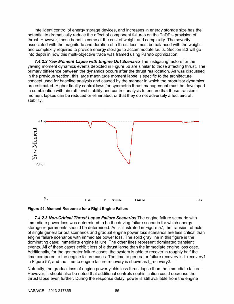
NASA/CR—2013-217865 86

Intelligent control of energy storage devices, and increases in energy storage size has the potential to dramatically reduce the effect of component failures on the TeDP’s provision of thrust. However, these benefits come at the cost of weight and complexity. The severity associated with the magnitude and duration of a thrust loss must be balanced with the weight and complexity required to provide energy storage to accommodate faults. Section 8.3 will go into depth in how this multi-objective trade was framed using Pareto optimization.

7.4.2.2 Yaw Moment Lapse with Engine Out Scenario The instigating factors for the yawing moment dynamics events depicted in Figure 56 are similar to those affecting thrust. The primary difference between the dynamics occurs after the thrust reallocation. As was discussed in the previous section, this large magnitude moment lapse is specific to the architecture concept used for baseline analysis and caused by the manner in which the propulsor dynamics are estimated. Higher fidelity control laws for symmetric thrust management must be developed in combination with aircraft level stability and control analysis to ensure that these transient moment lapses can be reduced or eliminated, or that they do not adversely affect aircraft stability.

Figure 56. Moment Response for a Right Engine Failure

7.4.2.3 Non-Critical Thrust Lapse Failure Scenarios The engine failure scenario with immediate power loss was determined to be the driving failure scenario for which energy storage requirements should be determined. As is illustrated in Figure 57, the transient effects of single generator out scenarios and gradual engine power loss scenarios are less critical than engine failure scenarios with immediate power loss. The solid gray line in this figure is the dominating case: immediate engine failure. The other lines represent dominated transient events. All of these cases exhibit less of a thrust lapse than the immediate engine loss case. Additionally, for the generator failure cases, the system is able to recover in roughly half the time compared to the engine failure cases. The time to generator failure recovery is t_recovery1 in Figure 57, and the time to engine failure recovery is shown as t_recovery2.

Naturally, the gradual loss of engine power yields less thrust lapse than the immediate failure. However, it should also be noted that additional controls sophistication could decrease the thrust lapse even further. During the response delay, power is still available from the engine

NASA/CR—2013-217865 87

depending on the time constant of engine power loss. When the failure is observed the thrust load is reallocated and the generator loads from the failed engine cease. This is evident by the sharp decrease in thrust directly after t_response. With no energy storage in the system, the power available from the system depends on the power available from the non-failed engine. The transient impact of this logic is shown by the dashed gray line in Figure 57, directly after t_response. If the nature of the engine failure is known, the sharp decrease may not be necessary and the max thrust lapse may be reduced.

t_0 t_failure t_response t_recover1 t_recover2 t_final

Immediate Engine Loss Max Lapse

Gradual Engine Loss Max Lapse

Generator 1 Failure Max Lapse

Generator 2 Failure Max Lapse

Thrust Required

Immediate Engine LossTransient Engine Power LossGenerator 2 FailureGenerator 2 Failure

Immediate Engine LossTransient Engine Power LossGenerator 2 FailureGenerator 2 Failure

Immediate Engine Power LossTransient Engine Power LossGenerator 1 FailureGenerator 2 Failure

Figure 57. Thrust Lapse Comparison Between Component Failures with No Energy Storage

t_0 t_failure t_response t_recover1 t_recover2 t_final

Immediate Engine Loss Max Lapse

Gradual Engine Loss Max Lapse

Generator 1 Failure Max Lapse

Thrust Required

Immediate Engine LossTransient Engine Power LossGenerator 2 FailureGenerator 2 Failure

Immediate Engine Power LossTransient Engine Power LossGenerator 1 FailureGenerator 2 Failure

Immediate Engine LossTransient Engine Power LossGenerator 2 FailureGenerator 2 Failure

Immediate Engine Power LossTransient Engine Power LossGenerator 1 FailureGenerator 2 Failure

Figure 58. Thrust Lapse Comparison Between Component Failures with Energy Storage

NASA/CR—2013-217865 88

When energy storage is added to the system, the immediate engine failure remains the dominant failure case as illustrated in Figure 58. The magnitude of the thrust lapse associated with the immediate engine loss is the greatest. However, it has reduced to the magnitude that occurred for the generator 1 failure scenario.

Regardless of energy storage available, this case continues to generate dominant transient thrust loss events. Therefore, this event was used to determine energy storage requirements. The process for this energy storage sensitivity study is discussed in Section 8.2.

7.5 Modeling Section Review

This section outlined the overall methodology applied for system modeling and simulation. The models are discussed at length and the type of dynamic outputs which are monitored to evaluate system performance. The fidelity and breadth of study results presented in the next sections are affected by assumptions outlined in this section.

The selection of power flow modeling instead of through and across variable representations introduced limitations in the way system dynamics could be approximated. Additionally, failures were expressed generally, in terms of loss of power, not in terms of effects on torque, speed, inertia properties, voltage, current, or other physical attributes of the system.

Some dynamic events discussed in this section are a direct result of the control logic implemented for this system. These include adverse yaw moments during acceleration, additional thrust lapse after the response delay when additional power from the failing component is available. Additionally, power flow models made modeling of the energy storage charge and discharge logic challenging because the control laws could not be conditioned around bus voltages.

This section also introduced the dynamic features which are used to identify the sensitivity of system performance to component attributes. Additionally, justification was given for applying specific focus on two scenarios during sensitivity analysis: step change in thrust demand, and rapid engine power loss. Generator failure scenarios were shown to be dominated by engine failure scenarios for this architecture. Additionally, the challenges associated with capturing TeDP yaw moment requirements were discussed in this section. Gust and stability augmentation scenarios were not targeted for sensitivity analysis. In order to perform these system design trade studies, future work is required to integrate the modeling and analysis of a TeDP system dynamics and the N3-X aircraft stability and control.

NASA/CR—2013-217865 89

8. System Sensitivity Study

Task1.e The Contractor shall develop a dynamic system model for the architecture chosen in d. and use the system model to assess the system issues chosen for study in the Task Task1.f The requirement, if any, for energy storage shall be assessed with respect to type and capacity and the general requirements for a control system shall be determined.

Sensitivity/uncertainty analysis was performed on this N3-X TeDP architecture model to determine which component attributes have the largest effect on the system’s transient thrust performance and engine failure response. The framework for this analysis followed the LibertyWorks parametric optimization process as illustrated in Figure 59. This process requires first, the integration of vehicle system models, second, an intelligent sampling of these models through design of experiments, third, meta-modeling, and finally, design space exploration.

The process illustrated in this figure includes a feedback loop in which technology solutions are selected and their specific benefits are assessed. However, for the purposes of this study, technology benefits analysis is omitted and the process ends with the sensitivity analysis.

The previous section discusses the first steps of this process: component and system modeling. This section discusses the design of experiments used for this study, the surrogate modeling, and finally, study results.

Figure 59. LibertyWorks Performance Optimization Process

8.1 Design of Experiments

A design of experiments requires model input variables which are characterized by their sampling ranges. For purposes of this study, exact values for these variables are unnecessary. Ranges for the system parameters are intended to get a reasonable feel for the impact of component performance on system dynamics.

NASA/CR—2013-217865 90

Tables 17 and 18 give the input parameters and their ranges for both the thrust response and engine out scenarios. Both scenarios are at an altitude of 5,200 ft and a standard day temperature offset of +27°F. The flight Mach number for these scenarios was set at 0.2. The conditions were set to represent a Denver, hot day conditions at takeoff and landing velocity. Thrust requirements were derived assuming a fan efficiency of 0.94%.

Table 17. DOE Variable Ranges for Thrust Response Sensitivity Analysis

Condition Value System Variable Range

Thrust_init 1000 lbf (approach) Reference Min Power 25000 40000 hp Thrust_final 55000 lbf (aborted landing) Engine/Gen Inertia 1 500 lb ft2 Alt 5200 ft ES 1_4 Pow 0.0001 100 (% of Bus Capability) Mach 0.2 ES 2_3 Pow 0.0001 100 (% of Bus Capability) DTamb +27 °F ES Energy 1_4 0.0001 10 (seconds ES @ full power) Peff 0.94 ES Energy 2_3 0.0001 10 (seconds ES @ full power) Engine TC 1 6 s Generator TC 0.01 0.5 s Energy Storage TC 0.01 0.05 s Propulsor TC 0.01 2.5 s Min Engine Speed 0.75 0.99 % speed Denver, Hot Day, Approach

The step change in thrust scenario is meant to represent the step change in thrust required for an aborted landing. The landing thrust was set at 1000 lbf due to model minimum thrust limitations. After the model reaches steady state conditions, the thrust required changes to 55,000 lbf (the estimated max thrust required for this vehicle [ref]).

Table 18. DOE Variable Ranges for Engine Power Loss Sensitivity Analysis

Condition Value System Variable Range

Thrust 55000 lbf (approach) Reference Min Power 25000 40000 hp Alt 5200 ft Engine/Gen Inertia 1 500 lb ft2 Mach 0.2 ES 1_4 Pow 0.0001 100 (% of Bus Capability) DTamb +27 °F ES 2_3 Pow 0.0001 100 (% of Bus Capability)

Peff 0.94 ES Energy 1_4 0.0001 10 (seconds ES @ full power)

ES Energy 2_3 0.0001 10 (seconds ES @ full power)

Engine TC 1 6 s Generator TC 0.01 0.5 s Energy Storage TC 0.01 0.05 s Propulsor TC 0.01 2.5 s Response Delay 0 2 s Min Engine Speed 0.75 0.99 % speed Denver, Hot Day, Takeoff

The flight conditions and system component variable ranges are the same for the two sensitivity studies. The engine loss scenario, however, is performed assuming a fixed 55,000 lbf thrust requirement. This requirement does not vary as the failure is imposed.

NASA/CR—2013-217865 91

Each simulation run involved 30 seconds of simulation time with a run time ratio of roughly 1:1 real time to simulation time. For each scenario, data was gathered with a 1200 run Latin hypercube design of experiments. Of these runs, 1000 were randomly selected to fit single hidden layer neural net regression with hyperbolic tangent activation functions. The remainder is used to assess model error checking.

All surrogate modeling, fit error checking, and data analysis was performed using the JMP (SAS Institute Inc.) software produced by SAS.

8.1.1 Thrust Response Scenario Neural Net Error Overview A regression for the time to 95% thrust recovery was made to determine the sensitivity of the

thrust response time to system parameters. Moment related regressions were not created because all moment loss dynamics are dominated by the propulsor control issues discussed in Section 7.4.1.

Multiple error checks were used to ascertain the accuracy of the fits used for this sensitivity analysis. Visual inspection of the predicted and residual plots, model fit and representation error histograms were used to determine accuracy. Additionally, the mean and standard deviation of these errors provided indication of fit.

Many sources for fitting inaccuracies may be present in these model fits. In addition to the error inherent in numeric fitting, the data to which the fit is made was generated by identifying dynamic features from a transient model. The tolerances for feature identification can introduce discrete jumps in the metric of interest. This is especially prevalent in recovery time estimates for energy limited simulation cases. As discussed in the previous section, energy limited cases may introduce secondary lapses in thrust. These lapses have the potential to defer the recovery time till seconds later.

While fitting inaccuracies do introduce challenges, this study is interested primarily in general trends and variable sensitivities. Exact fits are unnecessary and the fitting fidelity outlined in this section for this study is sufficient for our needs.

8.1.1.1 Error Analysis Time to 95% Thrust Recovery An 8-node, single-hidden-layer neural net regression was used to approximate the response time for the TeDP system to a step change in thrust demand. Figure 60 illustrates the error associated with the fit for this surrogate model. A model with a perfect fit would have all points lined up along the diagonal on the figure to the left, corresponding with zero residuals in the figure to the right. Red points on these plots represent the 200 points of hold back data which was not included in the neural net fits. The rest of the points were used to generate the surrogate model. The abscissa unit for these plots is given in seconds (the number of seconds till thrust is recovered).

The regression equation for the thrust step change scenarios are provided in Appendix B.

The data from these plots is distributed closely around the diagonal on the left plot in Figure 60. There are several outliers where the neural-net-predicted recovery time is too optimistic compared to the observed simulations. The outliers were investigated and seven of them were eliminated due to simulation issues.

Table 19 gives the model fit and representation error for this neural net regression. The model fit error (MFE) is the difference between the actual output and the predicted output for the points used to generate the fit. The model representation error (MRE) is the difference between the actual and predicted outputs for the hold back points not used in the fit. Both distributions are fairly normally distributed around zero and have a standard deviation is less than 0.4 seconds.

NASA/CR—2013-217865 92

8.1.2 Engine Failure Scenario Neural Net Error Overview Two neural net regressions were made for the sensitivity analysis of system performance

following an engine failure. The two outputs of interest were the magnitude of the thrust lapse incurred and the duration of the thrust loss following the failure. Engine failure scenarios affect propulsor performance symmetrically. Therefore, impacts on moment observed during this scenario were due to propulsor control issues, not loss in power available. These issues were observed and characterized in the thrust response study and are not repeated for engine failures.

Both regression equations for the engine out scenario are provided in Appendix C.

Figure 60. Thrust Response Model Prediction and Residual Error Compared to Simulation Outputs

Table 19. Model Fit and Representation Error for Thrust Response Recovery Time Thrust 95% Recovery MFE Thrust 95% Recovery MRE

-3 -2 -1 0 1 2 3

Stats

Mean 0.0008515 Std Dev 0.2446445 Std Err Mean 0.0077363 Upper 95% Mean 0.0160329 Lower 95% Mean -0.01433 N 1000

-3 -2 -1 0 1 2 3

Stats

Mean 0.0143568 Std Dev 0.3748512 Std Err Mean 0.026506 Upper 95% Mean 0.0666254 Lower 95% Mean -0.037912 N 200

NASA/CR—2013-217865 93

8.1.2.1 Error Analysis of Thrust Lapse A 10-hidden-node, single-layer neural net was

used to estimate the magnitude of the thrust lapse associated with an engine failure. The summary of the fit is given by Figure 61 and Table 20. The lapse was recorded in terms of percent thrust loss, with a max loss of roughly 50%. All axes in these figures are in units of percent.

In contrast to the step change in thrust data, the thrust lapse data for engine out scenarios exhibits significant groups or clusters. These groupings are indicated in Figure 61 and occur on thrust lapses ranges centered around 30% thrust loss and 50% thrust loss. Between these points the fit does an acceptable job at predicting the lapse. However, the data is more dispersed and less dense.

The cluster at 50% thrust loss occurs because this is the maximum thrust lapse that can occur assuming the other engine functions. Any combination of system parameters which is insufficient to provide fill-in power and to respond quickly to the failure will have a thrust loss at or near this limit.

The second cluster around 30% corresponds to the lapse which occurs when power is reallocated. This corresponds to a group of cases with moderate to long response time delays, high energy storage capacity on the inner bus, and moderate to low energy storage capacity on the outer bus. When the failure occurs, the central bus energy storage device is used to fill in the lost power for 3 of the propulsors. If the delay is too long, the energy storage device is energy limited. Therefore, before power is reallocated to the inner bus, the resulting lapse is roughly 30% of the total power.

Model fit and representation errors are given in Table 20. The standard deviation of the error is less than 3.5 percent and the error is distributed with a slight positive offset of the mean.

All of the regressions reviewed in this report are used to determine the sensitivity of the system response to transient requirements in terms of system attributes. However, because the engine failure scenario introduces the most taxing energy storage requirements, this regression will also be used to determine the trade-off between loss of thrust and energy storage weight.

20

30

40

50

Pre

dict

ed M

ax

Thru

st L

apse

10 20 30 40 50

Max Thrust

Lapse

-40

-30

-20

-10

0

10

20

30

40

Max

Thr

ust

Laps

e E

rror

10 20 30 40 50

Max Thrust

Lapse Figure 61. Thrust Lapse Prediction and Residual Error Compared to Simulation Outputs

NASA/CR—2013-217865 94

Table 20. Model Fit and Representation Error for Engine Failure Thrust Lapse Magnitude Thrust Lapse MFE Thrust Lapse MRE

-15 -10 -5 0 5 10 15

Stats

Mean -0.056786 Std Dev 3.0535387 Std Err Mean 0.0965614 Upper 95% Mean 0.1326999 Lower 95% Mean -0.246273 N 1000

-15 -10 -5 0 5 10 15

Stats

Mean 0.1437117 Std Dev 3.4950489 Std Err Mean 0.2471373 Upper 95% Mean 0.6310557 Lower 95% Mean -0.343632 N 200

8.1.2.2 Error Analysis of Time to 95% Thrust Recovery The second 10 hidden node neural-net was made to estimate the time to recover 95% of the required thrust when an engine failure occurs. The error associated with these fits is illustrated in Figure 62 and Table 21. All axes in these figures are in units of time in seconds.

As is apparent from the disperse nature of the points in this figure, the complex dynamics of the system and the ability to accurately identify a recovery make fitting difficult. While a trend can be identified, regressions generated from this data are insufficient to be used as a predictive model. The main factors which impact recovery time are discussed in Section 4.2.2.

Model fit and representation errors for this surrogate model are given in Table 21.

1

2

3

4

5

6

Pre

dict

ed T

ime

to

95%

Thr

ust R

ecov

ery

1 2 3 4 5 6 7

Time to 95%

Thrust Recovery

-6

-5-4-3

-2

-101

23

456

Tim

e to

95%

Thr

ust

Rec

over

y E

rror

1 2 3 4 5 6 7

Time to 95%

Thrust Recovery Figure 62. Thrust Lapse Prediction and Residual Error Compared to Simulation Outputs

NASA/CR—2013-217865 95

Table 21. Model Fit and Representation Error for Thrust Response Recovery Time Thrust 95% Recovery MFE Thrust 95% Recovery MRE

-3 -2 -1 0 1 2 3

Stats Mean 0.0115621 Std Dev 0.6594549 Std Err Mean 0.0208538 Upper 95% Mean 0.0524844 Lower 95% Mean -0.02936 N 1000

-5 -4 -3 -2 -1 0 1 2 3 4

Stats Mean 0.0657737 Std Dev 1.1728885 Std Err Mean 0.0829357 Upper 95% Mean 0.2293194 Lower 95% Mean -0.097772 N 200

8.2 Sensitivity Analysis Results

In order to understand the dynamics of the system and what drives system transient performance, the neural net regressions were used to identify which factors impact system dynamic performance the most.

8.2.1 Step Change in Thrust As is apparent from Figure 63, the propulsor and engine time constants are the primary

drivers for the transient response of the aircraft to a demand in thrust for the aborted landing scenario. Figure 63 shows a sensitivity profile for the thrust response output in terms of all system variables. Each window in this chart is a two dimensional slice of the neural net discussed in Section 8.1.1. This row of graphs shows the variation in time to 95% thrust available as a function of each of the system parameters independently. From this figure, it is observed that an increase or decrease in either of these two factors yield similar effects on the thrust response.

1

2

3

Pred

icte

d Ti

me

t%

Thru

st R

ecov

e1.

7289

48

0 1 2

1Energy_Storage_1_4_energy

(s)

0 1 2

1Energy_Storage_2_3_energy

(s)

0 3 6 9 12

5ES1_4

Power (MW)

0 10

5ES2_3

Power (MW)

010

020

030

040

050

0

150Engine_Inertia

(lb * ft^2)

0.8

0.9 1

0.9MinEngSpeed

(%)

3000

0

3500

0

4000

0

30000Full_System_Min_Power

(hp)

0.01

0.02

0.03

0.04

0.05

0.01Energy_Storage_Tc

(s)

1 2 3 4

3Engine_Tc

(s)

00.

10.

20.

30.

40.

5

0.1Generator_Tc

(s)

0 1 2

1.3Propulsor_Tc

(s) Figure 63. Independent Effects of System Parameters on Thrust Response

These results come as no surprise. Given each factor independently, the propulsor is the only component whose response rate is guaranteed to affect propulsor response. Additionally, the engine time constant may affect thrust response if it is longer than that of the propulsor and insufficient energy storage capability is available.

The importance of the propulsor and engine time constants is also illustrated in Figure 64. This figure contrasts the effect of each independent variable on the response and gives rank order to the impact of each factor given the range over which it was exercised. Logically, the

NASA/CR—2013-217865 96

first two factors, propulsor time constant and engine time constant, account for more than half of the variability associated with the thrust response scenario.

Thrust Step Change (Time to 5% Thrust Lapse)(Denver, Hot Day, Touch and Go)

Propulsor_Tc (s)

Engine_Tc (s)

Full_System_Min_Pow er (hp)

Energy_Storage_1_4 DischargeDuration (s)

ES1_4 Pow er (MW)

ES2_3 Pow er (MW)

Energy_Storage_Tc (s)

Energy_Storage_2_3_DischargeDuration (s)

MinEngSpeed (%)

Generator_Tc (s)

Engine_Inertia (lb * ft^2)

Relative Factor Contrast Magnitude Figure 64. TeDP System Component Capability Importance for Thrust Response

The step change in thrust requirements for an aborted takeoff illustrates the relative impact of each of the system parameter and the importance of propulsor response and engine response metrics. However, it does not introduce sizing critical energy storage trades. None of the cases simulated for this scenario failed to achieve the 5 seconds to go from flight idle to 95% thrust required. This includes cases which included very little to no energy storage available.

Each individual engine is sized to provide 100% of the required thrust. Assuming each engine can accelerate from idle to 95% thrust in 5 seconds as specified by FAR requirements, then the combined acceleration of two engines is more than sufficient. The thrust response capability can be achieved without the addition of energy storage devices. Additional maneuverability may be available with energy storage, but energy storage devices are not performance critical for the thrust response scenario.

Sensitivity results do provide insight into which energy storage devices are more critical to increase response time, if desired. From Figure 64, we see that the charge capacity of the outer bus energy storage devices (Energy_Storage_1_4 Discharge Duration) is more critical to thrust response than the capacity of the inner bus energy storage devices (Energy_Storage_2_3 Discharge Duration) for this architecture. Considering the step-change-in-thrust-demand scenario in isolation, energy storage on the outer buses is preferable to energy storage on the inner buses.

NASA/CR—2013-217865 97

8.2.2 Engine Failure The sensitivity analysis considered the effect of system parameters on the magnitude and

duration of thrust loss during an engine failure scenario. Using the regressions discussed in Section 8.1.2, Figure 65 shows the impact of each system parameter on both the maximum thrust loss incurred and the time it takes to recover 95% of the original thrust requirement.

Consider first the trends associated with recovery time as profiled in the first row in Figure 65. The results in this row are not intended to denote exact results, but rather to show the general effects of the system parameters on the recovery time.

In contrast to the previous scenario, engine time constant and energy storage parameters critically affect on the time to recover thrust. For the engine loss scenario, emphasis is placed on providing un-interrupted power to the propulsor. Hence the emphasis placed on energy storage factors, system delay, and the sizing parameters. The propulsors need not accelerate and decelerate with a fast time constant.

1

3

5

7

Pred

icte

d Ti

me

to%

Thr

ust R

ecov

3.43

7284

10

20

30

40

Pred

icte

d M

axTh

rust

Lap

se28

.196

22

0 1 2

1Delay (s)

0 1 2

1Energy_Storage_1_4_energy

(s)

0 1 2

1Energy_Storage_2_3_energy

(s)

0 3 6 9 12

5ES1_4

Power (MW)

30,0

0032

,000

34,0

0036

,000

38,0

0040

,000

35,000Full_System_Min_Power

(hp)

0 10

5ES2_3

Power (MW)

010

020

030

040

050

0

150Engine_Inertia

(lb * ft^2)

0.8

0.9 1

0.9MinEngSpeed

(%)

0.01

0.02

0.03

0.04

0.05

0.03Energy_Storage_Tc

(s)

1 2 3 4

3Engine_Tc

(s)

00.

10.

20.

30.

40.

5

0.1Generator_Tc

(s)

0 1 2

1Propulsor_Tc

(s) Figure 65. Independent Effects of System Parameters on Thrust Recovery

Contrasting the first and second rows in Figure 65, the propulsor time constant has a large effect on the magnitude of the thrust loss incurred during failure. However, a large time constant propulsor is advantageous for this case. With a long time constant, the thrust does not lapse as quickly, allowing more flexibility in providing fill-in power and engine response. The time constant at which the engine responds has a limited effect on the magnitude of the loss. The magnitude of the loss is also not affected by increasing the overall system capacity.

Figure 66 ranks the system parameters in terms of the variability of both the thrust loss magnitude and recovery delay. Engine time constant has the largest impact on the lapse duration and the inner bus energy storage device has the largest impact on the magnitude of the lapse. As expected, the effect of system delay is great. The thrust required cannot be provided until the recovery logic has been engaged. While all other parameters affect this metric through the system dynamics, the delay acts as a time offset during which energy storage capacity is depleted.

NASA/CR—2013-217865 98

Engine Out (Time to 5% Thrust Lapse)(Denver, Hot Day, Takeoff)

0 0.1 0.2 0.3 0.4 0.5 0.6 0.7

Engine_Tc (s)

Delay (s)

ES2_3 Power (MW)

Energy_Storage_2_3_energy(s)

Energy_Storage_1_4_energy(s)

ES1_4 Power (MW)

Propulsor_Tc (s)

Engine_Inertia (lb * ft 2̂)

Generator_Tc (s)

MinEngSpeed (%)

Energy_Storage_Tc (s)

Factor Importance

Engine Out (Magnitude of Thrust Loss)(Denver, Hot Day, Takeoff)

0 1 2 3 4 5 6

ES2_3 Power (MW)

Delay (s)

Energy_Storage_2_3_energy(s)

ES1_4 Power (MW)

Energy_Storage_1_4_energy(s)

Propulsor_Tc (s)

MinEngSpeed (%)

Energy_Storage_Tc (s)

Engine_Tc (s)

Engine_Inertia (lb * ft 2̂)

Generator_Tc (s)

Factor Importance Figure 66. TeDP System Component Capability Importance for Thrust Recovery

Figure 66 again indicates which energy storage device has a greater impact on system dynamics. While the thrust demand prefers energy storage on the outer buses, the engine out scenario prefers energy storage available on the inner bus. However, both inner and outer energy storage devices can have a large impact on the magnitude of the lapse. Both devices are needed to fill in power during the system delay. In addition, the inner energy storage must continue to fill in power after power has been reallocated.

Energy storage benefits come at a cost of weight to the system. Although fill-in power is required for only a few seconds during engine failure, the weight of an energy storage system can be significant. The benefits of reducing thrust lapse must be balanced with the potential impacts on weight.

8.3 Energy Storage Pareto Optimization

There is a threshold for improvement and a point of diminishing return for the energy storage system in terms of energy and power. Consider the effect of energy storage capacity on the predicted thrust lapse (max_TLapse) occurring with engine failure which is depicted in Figure 67. The areas of interest are highlighted in red for the energy storage discharge time on the inner (Energy_2_3(s)) and outer (Energy_1_4(s)) buses. These example profiles reflect the conditions: system response delay equal to 2 seconds, all energy storage devices sized at 5 MW rating, propulsor time constant of 1 second, and an engine time constant of 4 seconds. The ranges indicated on this figure float depending on the values of the other system parameters.

Looking at the outer bus energy storage devices (ES Energy_1_4(s)), there is little benefit to having less than 5 MW-s an energy storage capacity. On the other hand, energy storage capacities or greater than roughly 15 MW-s provide no additional benefit in terms of the magnitude of thrust lapse compared with the cost of additional weight. Similar ranges are observed for the inner bus energy storage device. For the parameter values used in this figure, energy storage on the inner bus need not exceed roughly 6 MW-s capacity because no additional benefit in thrust lapse reduction is achieved.

NASA/CR—2013-217865 99

Figure 67. Area of Interest for Energy Storage Capacity

The two competing objective (minimize weight, minimize thrust lapse) can be balanced by varying the extent to which energy storage is used as illustrated in Figure 68. Ideally, the system would exhibit no thrust lapse and incur no cost in terms of energy storage weight. This ideal point is indicated by the star at the origin in this figure. While this point is desirable, it is not feasible or viable. A compromise must be made depending on the importance of both of these metrics.

Thrust Lapse

Ener

gy S

tora

ge W

eigh

t

00

Max LapseMin Weight

Min LapseMax Weight

ParetoOptimal

Figure 68. Notional Pareto Front for Thrust Lapse versus Energy Storage Weight Trades

The blue and green points on this figure represent the desired solutions under different specific preferences. If minimizing weight is the only weighted objective to be achieved regardless of the impact on thrust lapse, then the green point on the lower right corner of the graph would be the decided ideal. Conversely, if system weight is insignificant and the minimizing thrust lapse is crucial then the blue point on the upper left would be the selection. In reality there is a tradeoff between the two metrics which is limited by the physics of the problem. Pareto optimal solutions represent the best set of compromises. For these solutions, there is no way of making improvements to one metric without expense to another. From a Pareto optimal set of solutions, a Pareto front can be identified. This Pareto front is represented by the red dashed line in Figure 68. This Pareto front of best compromises characterizes the tradespace between the two metrics.

NASA/CR—2013-217865 100

To characterize these trades, a series of optimizations runs was performed on the neural net regression for thrust lapse magnitude discussed in Section 8.1.2. The independent variables for these optimizations were the sizing parameters for both outer and inner bus energy storage devices (power rating, and total capacity). Using the surrogate model for dynamic performance, the expected thrust lapse (TLapse) for an engine out scenario was estimated. By assuming energy and power density values for the energy storage devices, the total energy storage weight (WES) was also estimated. The optimization objective function takes the form:

]1,0[,]1,0[,1 ,__

∈∈=++= BABAW

WBT

TAObj

refES

ES

refLapse

Lapse (19)

Optimizations were performed by varying the preferences between weight and lapse minimization. The A and B values in Equation (19) are the weighting values for the two objectives. The values for TLapse_ref and WES_ref were set to normalize the thrust lapse and weight values and were given the values of 50% and 500 kg, respectively.

DCTBT

AW lapseLapse

ES +−−

= (20)

The optima were filtered to reduce clustering of solutions and to identify all Pareto solutions. From these solutions, a regression was made to numerically approximate the Pareto front. The form of this regression follows Equation (20).

Figure 69 illustrates the data processing used in this process. The weights and lapses illustrated in this figure were generated at a specific setting of system parameters and values for energy storage specific power and energy. This figure is meant for illustrative purposes only.

Figure 69. Example Energy Storage Pareto Front for Engine Power Failure at Takeoff

All the points on this graph represent an optimum obtained for one setting of the weighting values. Due to the non-convex nature of the objective function and potentially ill-tuned convergence criteria, not all of the points found by the optimizer were Pareto optimal. The non-Pareto optimal points were eliminated and are depicted with a blue ring around each dominated point in Figure 69. Pareto optimal points in this figure are displayed in solid green and the Pareto front was estimated by the regression given by the red line.

NASA/CR—2013-217865 101

From the Pareto front estimate in Figure 69, there is fairly linear relationship between the magnitude of the thrust lapse and the weight of the energy storage devices for large thrust lapses. However, for low values of thrust lapse improvements, there is a point of diminishing return. The energy storage weight increases asymptotically as it approaches some low end thrust lapse limit.

The effect of system parameters on this Pareto front was captured by running series of optimizations with one-at-a-time factor variation. Eleven Pareto fronts were identified to characterize the five variables most significant to thrust lapse magnitude: energy storage specific power, energy storage specific energy, system response delay, engine time constant, and propulsor time constant. The parameter values and ranges used here are given in Table 22.

Table 22. Design of Experiments Factors and Ranges for Energy

Storage Pareto Optimum Analysis

Factors Factor Ranges Low Med High

A Specific Energy (W×h/kg) 50 150 250 B Specific Power (kW/kg) 20 70 120 C Response Delay (s) 0 1 2 D Propulsor Time Constant 0.1 0.5 1 E Engine Time Constant (s) 2 4 6 Engine Inertia (lb×ft2) - 150 - Yaw Moment (ft×lb) - 0 - Min Engine Speed (%) - 85 - Energy Storage Time Constant (s) - 0.01 - Generator Time Constant (s) - 0.1 - System Reference Power Rating

(hp) - 30,000 -

The medium range is used as the baseline case for this sensitivity evaluation. Results are plotted in Figure 70 A through E. Each plot in this figure corresponds to the case indicated in Table 22.

Regardless of the factor parameters evaluated, hundreds of kilograms of energy storage are necessary to yield the maximum reduction in thrust lapse during engine out. However, these plots show that partial mitigation of thrust lapse is available with a lesser weight cost. Additional studies are necessary to extend this Pareto analysis to consider additional dimensions of this thrust lapse trade. More accurate estimates of thrust lapse duration would be necessary to perform this analysis.

NASA/CR—2013-217865 102

0

100

200

300

400

500

600

700

0 10 20 30 40 50 60

Wei

ght(k

g)

Thrust Lapse (%)

A.

ES Energy Density (Wh/kg)=50ES Energy Density (Wh/kg)=150ES Energy Density (Wh/kg)=250

0

100

200

300

400

500

600

700

0 10 20 30 40 50 60

Wei

ght(k

g)

Thrust Lapse (%)

B.

ES Power Density (kW/kg)=20ES Power Density (kW/kg)=70ES Power Density (kW/kg)=120

0.00E+00

5.00E+01

1.00E+02

1.50E+02

2.00E+02

2.50E+02

3.00E+02

3.50E+02

4.00E+02

0 10 20 30 40 50 60

Wei

ght(k

g)

Thrust Lapse (%)

C.

Delay (s)=2Delay (s)=1Delay (s)=0.5

0.00E+00

5.00E+01

1.00E+02

1.50E+02

2.00E+02

2.50E+02

3.00E+02

3.50E+02

4.00E+02

0 10 20 30 40 50 60

Wei

ght(k

g)

Thrust Lapse (%)

D.

Propulsor TC (s)=1Propulsor TC (s)=0.5Propulsor TC (s)=0.1

0

50

100

150

200

250

300

350

400

450

500

0 10 20 30 40 50 60

Wei

ght(k

g)

Thrust Lapse (%)

E.

Engine TC (s)=6Engine TC (s)=4Engine TC (s)=2

Figure 70. Sensitivity of Pareto Optimal Energy Storage Weight versus Thrust Lapse to Technology Factors

As is to be expected from the sensitivity study, variations in the energy storage energy and power density yield the largest impact on the energy storage tradespace. The effects of these parameters on the Pareto fronts are non-linear. This is observed by the larger displacement between the blue and green curves than between the orange and blue curves in Figures 70-A and B.

NASA/CR—2013-217865 103

Additionally, the duration of the delay between failure and thrust reallocation has a large effect on the energy storage weight versus lapse Pareto fronts. However, the response delay must be less than 1 second to alter the tradespace. All l but one of the Pareto front from Figure 70 intercept the abscissa at roughly 50% thrust lapse. The only parameter which effects the zero energy storage weight thrust lapse is the response delay variable. While changes in the delay time from between 1 and 2 seconds has no impact on the energy storage tradespace, reducing the delay time to 0.5 seconds decreases the zero energy storage weight thrust lapse to 40%. Fast acting failure identification and thrust allocation response has a critical impact on the magnitude of hazard incurred during an engine out at takeoff failure scenario.

NASA/CR—2013-217865 104

9. Conclusions The N3-X aircraft concept has the potential to provide significant improvement in fuel

efficiency in pursuit of NASA’s N+3 goals. However, significant advances in component technology and systems integration remain for these benefits to be realized. This research effort endeavored to get a better sense of the critical transient performance issues for a TeDP electrical system, mature the TeDP system concept, identify technology gaps, and investigate the challenges of utilizing this system for flight critical thrust and control requirements.

9.1 Key Observations and Challenges

9.1.1 Issue Identification and Selection Initial issue identification required the identification of potential problems that originate within

the system or from the environment in which the system must operate. Each component within the system presents a significant number of design issues for safe and effective integration within the context of the system. Additionally, each flight phase introduces a variety of operational challenges for the electrical system. All issues were evaluated on a basis of probability that the event in question will occur, significance/severity of the requirements that are introduced by the event, triviality of the technical solution, and programmatic limitation of this research.

The issues selected for further evaluation were introduced in Table 6. The focus with this selection of issues is understanding the fundamental dynamic requirements of the TeDP system during scenarios that are either expected to take place for an aircraft (acceleration/deceleration, cross-wind, control) or have probable occurrence for a fleet of commercial aircraft (engine, generator failure). Many additional issues that present component design and system integration challenges were discussed and evaluated. These challenges must be addressed during concept design in order for this electrical power system to be sufficiently demonstrated.

(From Section 2.2) Table 1. Recommended Issues

Category Questions to be answered Issue

Nominal Operations

What is the baseline system performance?

What does the system need to look like?

Acceleration/Deceleration

Gust/Crosswind

Aircraft Control and Stability Augmentation

What is the role of energy storage? Identifying Energy Storage Requirements

Off-Nominal Operations

What is the system level effect?

Is this failure a design show-stopper?

What additional requirements need to be included?

Engine Shutdown

Loss of Energy Storage

Internal Short on Generator

A key observation from this issue identification and selection exercise regards the limitations of FAR 25 requirements in framing the critical failure requirements for this nontraditional commercial aircraft concept. Sizing critical requirements are derived from architecture specific off-nominal operating scenarios. In the case of this revolutionary system, traditionally applicable rules of thumb may not be sufficient in estimating required component size. While FAR does express some minimum levels of aircraft level performance that must be achieved during off-nominal states, the premise of these standards reflects the heritage of conventional tube-and-wing aircraft with podded propulsion. For a BWB with TeDP, standard failure cases like single-

NASA/CR—2013-217865 105

engine out at takeoff and bird strike present different challenges than those perceived and expressed by federal standards. The definition and evaluation of this flight critical vehicle system requires a departure from existing FAR requirement and a focus on the operational hazards that must be mitigated when failures occur. These evaluations should be performed concurrent to concept definition in order to accurately predict the sizing critical requirements for each component or subsystem.

9.1.2 Architecture Selection and Sizing 9.1.2.1 Contingency Requirements The identification of sizing critical scenarios was

required to compare the efficacy of the candidate architectures considered for this study. Therefore, a formal contingency analysis was performed for several candidate TeDP architectures. The level of system redundancy and interconnectivity was shown to affect which failure scenarios drive component requirements. Interconnectivity reduced the propulsor redundancy required to provide flight-critical thrust. However, the associated reduction in propulsor weight was counteracted by the equipment weight and system complexity associated with rerouting power during a failure condition.

9.1.2.2 Architecture Evaluation Four metrics were considered for architecture comparison: weight, component count, excess power available, and failure response complexity. While the inner bus tie architecture represented the best compromise between these considerations, all concepts exhibit advantageous attributes that may be preferable depending on the emphasis placed on each of the metrics. Both technology progress and changes in metric preferences must be projected in order to accurately select the right architecture.

The results of the architecture study, a review of current TeDP electrical system component technology, and a review of how technology may develop were presented. Superconducting or cryogenic electrical system component technology is progressing but still needs to improve in terms of power density in order for the N3-X aircraft to be possible. The type of superconducting electric machine, SFCL, converter, cable, protection, and energy storage as well as voltage level used for the N3-X aircraft all depend on the progression of technology to maximize power density and minimize system weight.

9.1.2.3 Differential Thrust The TeDP system power requirements and subsequent component weights are highly sensitivity to the magnitude of the yaw moment steady-state trim requirements. The inner bus tie architecture requires 40% propulsor oversizing to provide fail-safe performance. However, this oversizing will increase linearly with increases to the magnitude of yaw support provided by differential thrust. This is illustrated in Figure 71 which shows the ratio of the overall propulsor thrust available to the minimum takeoff thrust under varying aircraft directional control moments.

Trimming Differential Thrust Yaw Moment Required Figure 71. The Effect of Aircraft Directional Control Trimming on Propulsor Sizing

NASA/CR—2013-217865 106

Dynamic requirements for this system must also be considered when determining the extent to which differential thrust is used for yaw control. Latency, bandwidth, rate, and certification requirements for aircraft directional control on a BWB aircraft may prove challenging for a differential thrust only flight control solution. The magnitude of this challenge is highly dependent on propulsor technology progression.

Additional analysis is necessary to integrate dynamic aircraft performance analysis with that of the TeDP electrical system. This relationship between TeDP system dynamics and flight dynamics will govern the electrical system control requirements to avoid adverse moments. Propulsor acceleration must be synchronized and account for all non-linearities in aircraft performance, deviations due to boundary layer issues, and deviations due to component degradation. Additional work is necessary to configure the balance between traditional and differential thrust yaw control for static and dynamic moment requirements.

This study recommends assigning propulsors to central distribution buses in a symmetric fashion to minimize adverse yaw moments during electrical distribution system faults or failures. This was challenging given the number of propulsors for the baseline N3-X concept. With 14 or 15 propulsors, an odd number of propulsors was assigned to some of the buses for all candidate architecture considered. Bus number, propulsor number, and propulsor assignment must be considered during TeDP concept development. For simplicity, it is preferable that an even number of propulsors be assigned to each central distribution bus whenever possible.

9.1.2.4 Protection Systems Another key observation with this architecture study is the significant contribution of protection systems to overall architecture weight. Approximately 25% of the TeDP architecture weight can be attributed to protection equipment (note: weight trades did not include energy storage and SFCL weight). Depending on how technology progresses, the protection of the electrical system may rely more heavily on circuit breakers alone or SFCLs in conjunction with circuit breakers. The protection scheme also depends on whether the circuit breaker used is electromechanical or solid state.

9.1.3 System Modeling and Factor Sensitivity 9.1.3.1 System Modeling Initial assumptions were that power flow modeling would be

better to understand system and component requirements interaction. This proved accurate. The form of the models was sufficient to detail some high level system requirements. However, there were limitations to the types of conclusions that could be made based on the form of the model.

Component modeling and system integration was relatively simple by eliminating the necessity to enforce conservation throughout a complex system. However, defining the controls with no traditional state information posed difficulties especially for energy storage devices. Additionally, all failures had to be posed in terms of power flow. Future TeDP system developments should consider through and across variable modeling to explore additional safety critical scenarios. Benefits would include being able to represent failures in terms of more meaningful variables like torque, speed, and current. Additionally, some control strategies would be more easily implemented (engine inertia, energy storage). Different control issues would arise with through and across variable modeling, and charge and discharge logic would have to maintain intelligent use of energy storage.

Additional control challenges include the coordination of propulsor control to mitigate yaw lapses during thrust modulation and developing means for alleviating the fighting between energy storage devices (engine shaft inertia and bus energy storage).

9.1.3.2 Factor Sensitivity Analysis of the inner bus tie architecture concept discussed in the second deliverable showed the sensitivity of the TeDP system level transient performance in terms of the component level technology metrics.

NASA/CR—2013-217865 107

The propulsor and engine time constant values affected the variability of response time to thrust the most. The TeDP system had no challenge providing the idle to 95% thrust requirement within the allotted 5 seconds over all the ranges of technology parameters exercised. As such, energy storage is not necessary for thrust response. However, the use of energy storage has the potential to improve performance beyond the requirement as specified by FAR regulations.

The thrust lapse incurred during an engine out scenario with loss in engine shaft inertia imposed the most significant dynamic performance interruption compared to all other failure modes considered. The duration of the thrust lapse is highly sensitive to the engine time constant and the magnitude of the thrust lapse is sensitive primarily to energy storages attributes (power and energy ratings of the devices).

As is expected, the time constants of the electrical equipment have very little impact on the provision of thrust. This is due to the relative magnitude of these time constants compared to those for mechanical systems.

9.1.3.3 Energy Storage All FAR requirements may be met with no fill-in energy storage capability. Energy storage is not needed to provide the specified 5-second thrust response capability. Additionally, an engine out scenario with a conventional platform or with a TeDP system with no energy storage has the same effect. A 50% lapse will occur until the remaining engine accelerates to maximum thrust. However, including energy storage with a TeDP provides the ability to increase thrust response and curb the impact of component failures on thrust lapse. This added capability may not buy the energy storage system onto the platform by itself; however, the energy storage device has the ability to provide fail-safe redundancy to many functions simultaneously. Other roles of the energy storage device may include the support of engine start/restart capabilities, the provision of avionics, control, and/or auxiliary power for fail-safe operations, and the improvement of transient thrust response.

9.2 Future Work While no showstoppers were identified that refute the TeDP electric grid concept, many

challenges remain with regards to its design and implementation. Several avenues of continuing research in this area are discussed in the following subsections.

9.2.1 Vehicle Level Requirements Update The results of this study should be used to update the system level performance models of

the aircraft. Weight estimates of the electrical system should be updated to include the oversizing considerations of the propulsors for fault tolerant provision of thrust and yaw trimming. This overall weight must include approximations of all electrical equipment weight, including protection devices. Propulsor size has an impact on the number of propulsor devices used on the aircraft. Decreasing the maximum thrust rating of the propulsors allows for reductions in the fan area required. As the fan diameter shrinks, the number of propulsors that fit spanwise on the BWB increases. The results of adding propulsors include increased redundancy of the propulsors and increased responsiveness due to decreased propulsor inertia.

The impact of the electrical systems architecture on the other vehicle systems must also be assessed. In particular, the TeDP electrical system and cryogenic systems architecture designs are highly interdependent. The structure, composition, spatial integration, and interoperability of these two systems should be determined via a coordinated multidisciplinary architecting effort. Safety, reliability, and stability analysis must be performed for these two systems in combination to determine feasibility of the N3-X TeDP concept. Architecture trades should consider nonpropulsive power requirements, variations in number and placement of the engines and propulsors, and an expansion of the metrics used for concept evaluation (performance, cost, maintenance, complexity, integration into the current air traffic system, etc).

NASA/CR—2013-217865 108

9.2.2 Directional Control Modeling and Trade Studies A second area that must be addressed to mature the N3-X TeDP concept is the extent to

which differential thrust is used to support aircraft directional control requirements. Providing yaw control via differential thrust is aerodynamically attractive with drag inducing vertical tails and control surfaces removed. Additionally, the size, weight, complexity, and power demand from the control system can be dramatically reduced. However, these benefits come at significant cost. This study indicated the magnitude of the yaw moment provided by differential thrust has a large impact on the propulsor and electrical system sizing. Additionally, response rates required for fast acting directional stability augmentation may pose challenging for differential thrust concepts.

A dedicated research effort is required for developing the N3-X directional control system. This study should consider alternative flight control methods for providing both dynamic control response and steady-state trimming for directional control. Potential solutions may consider combination of differential thrust (e.g., propulsor speed modulation, variable pitch fans, variable guide vanes, and fan duct geometry manipulation), vectored thrust, and aerodynamic control (e.g., vertical surfaces, spoilers, split flaps).

Aircraft level considerations may also be considered in differential control concept trades. These may include propulsor placement and inboard versus outboard throttling. The selection of the preferred directional controls architecture must consider integrated dynamic analysis of the propulsors, TeDP system, and aircraft. Other significnant factors include overall system weight, complexity, and safety.

9.2.3 Architecture Modeling Assessing the failure response characteristic in this study was performed with simple power

flow models. While this allowed for the characterization of component requirements sensitivities, all failures were imposed and observed in terms of a loss in power available or provided. Therefore, increased model fidelity is recommended to enable more physically representative insertion and observance of failures. This will assist in developing the unit and non-unit protection strategies necessary to sense and respond to a failure. Additionally, constructing these models will allow for the development of detailed control laws for this TeDP electrical grid.

9.2.4 Protection and Control Studies The architecture definition and selection exercises discussed in this document

recommended the inner bus-tie TeDP architecture as the best compromise architecture. However, additional weight benefits may be achieved by increasing redundancy and interconnectivity. Failure accommodation with these more complex architecture concepts requires the development of more extensive logic for load allocation and power rerouting. It is therefore recommended that further studies look at the implementation of more advanced protection strategies for these highly interconnected concepts. Coupled with more detailed system models, logic should be developed that monitors failures in terms of system states (e.g., voltage, current, torque, and speed).

Failure analysis should also extend to consider interactions between vehicle systems and include common cause failure considerations.

9.2.5 Wholly Cryogenic System Demonstrator The final recommendation for future work relates to the fundamental research necessary to

progress superconducting electrical components to maturity. While research and development has been done to develop individual cryogenic, superconducting technologies, the implication of integrating all of these components in a wholly-cryogenic, superconducting system has not been fully evaluated. As such, it is recommended that plans should be put forth for the development

NASA/CR—2013-217865 109

of a laboratory demonstrator of a wholly-superconducting electrical system. This demonstrator need not reflect all of the redundancy and interconnectivity recommended for the candidate architectures in this study, but it must reflect the basic structure of the system as is illustrated in Figure 72.

Construction of this proof of concept system represents a large undertaking, but would act as a test bed for future technology developments and assist in maturing this TeDP concept towards a 2035 EIS date. Such a demonstrator would not only increase component technology readiness, but also answer questions concerning the integration, maintenance, and cooling of these technologies in a wholly superconducting system environment. This recommended future research work would help identify the limitations of such a system and other unknowns that must be accounted for in TeDP design.

N.O.N.O.

SCFCL SCFCL

Zone1

Zone2

Zone3

Zone4

Zone5

Zone6

Zone7

Figure 72. TeDP Protection Equipment Zones

NASA/CR—2013-217865 111

Appendix A. Candidate Architectures

Energy Storage

N.O.

N.O.

GL-1 GL-2

SCFCL SCFCL N.O.

GR-2 GR-1

SCFCL SCFCL

SCFCL

Energy Storage

N.O. SCFCL

Energy Storage

N.O.SCFCL

Energy Storage

N.O. SCFCL

14.3% 14.3% 14.3% 14.3%

ML-1 MR-1 ML-5 MR-5

14.3% 14.3% 14.3%

ML-4 MR-4 ML-7

14.3% 14.3% 14.3%

MR-7 ML-3 MR-3

14.3% 14.3% 14.3% 14.3%

ML-2 MR-2 ML-6 MR-6

57.2% 42.9% 42.9% 57.2%

57.2% 42.9% 42.9% 57.2%

14.3% 14.3% 14.3% 14.3% 14.3% 14.3% 14.3% 14.3%14.3% 14.3% 14.3% 14.3% 14.3% 14.3%

Left

Eng

ine

Right Engine

Right Side

Left Side

Energy StorageEnergy

Storage

Energy

StorageEnergy Storage

Superconducting FaultCurrent Limiter

Electric Machin SCFCL & AC/DC Converter

AC/DC Converter Energy StorageDevice

DC/AC Motor Drive Circuit Breakers

Energy Storage

SCFCL

SCFCL

Energy StorageEnergy

Storage

Energy

StorageEnergy Storage

Figure 73. Baseline Architecture (Diagrams not to Scale)

NASA/CR—2013-217865 112

Energy Storage

N.O.

N.O.

GL-1 GL-2

SCFCL SCFCL N.O.

GR-2 GR-1

SCFCL SCFCL

SCFCL

Energy Storage

N.O. SCFCL

Energy Storage

N.O.SCFCL

Energy Storage

N.O. SCFCL

10% 10% 10% 10%

ML-1 MR-1 ML-5 MR-5

10% 10% 10%

ML-4 MR-4 ML-7

10% 10% 10%

MR-7 ML-3 MR-3

10% 10% 10% 10%

ML-2 MR-2 ML-6 MR-6

SCFCL

N.O.

N.O.

10% 10% 10% 10% 10% 10% 10% 10%10% 10% 10% 10% 10% 10%

40% 60% 60% 40%

40% 60% 60% 40%

Left

Eng

ine

Right Engine

Right Side

Left Side

Energy StorageEnergy

Storage

Energy

StorageEnergy Storage

Superconducting FaultCurrent Limiter

Electric Machin SCFCL & AC/DC Converter

AC/DC Converter Energy StorageDevice

DC/AC Motor Drive Circuit Breakers

Energy Storage

SCFCL

SCFCL

Energy StorageEnergy

Storage

Energy

StorageEnergy Storage

Figure 74. Inner Bus Tie Architecture (Diagrams not to Scale)

NASA/CR—2013-217865 113

Energy Storage

N.O.

N.O.

GL-1 GL-2

SCFCL SCFCL N.O.

GR-2 GR-1

SCFCL SCFCL

SCFCL N.O. SCFCL

Energy Storage

N.O.SCFCL

Energy Storage

N.O. SCFCL

ML-1 MR-1 ML-5 MR-5 ML-4 MR-4 ML-7 MR-7 ML-3 MR-3 ML-2 MR-2 ML-6 MR-6

8.33% 8.33% 8.33% 8.33% 8.33% 8.33% 8.33% 8.33%8.33% 8.33% 8.33% 8.33% 8.33% 8.33%

8.33

%

5.56

%

5.56

%

4.17

%

8.33

%

8.33

%

5.56

%

8.33

%

4.17

%

4.17

%

4.17

%

8.33

%

8.33

%

8.33

%

50% 50% 50% 50%

50% 50% 50%

8.33

%

5.56

%

8.33

%

8.33

%

4.17

%

5.56

%

5.56

%

8.33

%

8.33

%

8.33

%

8.33

%

4.17

%

4.17

%

4.17

%

Left

Eng

ine

Right Engine

Right Side

Left Side

Energy Storage

Energy Storage

Energy

Storage

Superconducting FaultCurrent Limiter

Electric Machin SCFCL & AC/DC Converter

AC/DC Converter Energy StorageDevice

DC/AC Motor Drive Circuit Breakers

Energy Storage

SCFCL

SCFCL

Energy Storage

Energy Storage

Energy

Storage

Figure 75. 3-Bus Multi-Feeder Architecture, Dashed Feeder Lines Indicate the Secondary Connections (Diagrams not to Scale)

NASA/CR—2013-217865 114

Energy Storage

N.O.

N.O.

GL-1 GL-2

SCFCL SCFCL N.O.

GR-2 GR-1

SCFCL SCFCL

SCFCLEnergy Storage

N.O.SCFCL

Energy Storage

N.O.SCFCL

Energy Storage

N.O.SCFCL

ML-1 MR-1 ML-5 MR-5 ML-4 MR-4 ML-7 MR-7 ML-3 MR-3 ML-2 MR-2 ML-6 MR-6

8.33% 8.33% 8.33% 8.33% 8.33% 8.33% 8.33% 8.33%8.33% 8.33% 8.33% 8.33% 8.33% 8.33%

8.33

%

4.17

%

4.17

%

4.17

%

8.33

%

8.33

%

2.77

%

8.33

%

2.77

%

2.77

%

2.77

%

8.33

%

8.33

%

8.33

%

8.33

%

4.17

%

8.33

%

8.33

%

4.17

%

2.77

%

2.77

%

8.33

%

8.33

%

8.33

%

8.33

%

4.17

%

4.17

%

4.17

%

50% 50% 50% 50%

33.3% 33.3% 33.3% 33.3%

Left

Eng

ine

Right Engine

Right Side

Left Side

SCFCL

N.O.SCFCL

N.O. N.O.SCFCL

N.O.SCFCL

50% 50% 50% 50%

33.3

3%

33.3

3%

16.6

7%

33.3

3%

33.3

3%

16.6

7%

16.6

7%

16.6

7%

Energy Storage

Energy

StorageEnergy Storage

Energy

Storage

Superconducting FaultCurrent Limiter

Electric Machin SCFCL & AC/DC Converter

AC/DC Converter Energy StorageDevice

DC/AC Motor Drive Circuit Breakers

Energy Storage

SCFCL

SCFCL

Energy Storage

Energy

StorageEnergy Storage

Energy

Storage

Figure 76. Cross-Redundant Multi-Feeder Architecture, Dashed Feeder Lines Indicate the Secondary Connections (Diagrams not to Scale)

NASA/CR—2013-217865 115

Appendix B. Thrust Response Regression Equation This single hidden layer neural net regression with hyperbolic tangent activation functions

calculates the time to achieve 95% thrust required for the step change in thrust demand thrust response scenario.

T95 = 3.0020306364202 …

+ 0.362006816139137 * Tanh(…

0.5 * (12.8362451435072 + -0.489485952500546 * ES1_4_energy …

+ -0.818854667529427 * ES2_3_energy + 0.104404699391162 * ES1_4_power …

+ -0.124478063141393 * ES2_3_power + -0.00277232050886049 * Engine_Inertia …

+ -3.11059390801946 * EngSpeedMin + -0.0003354208208423 * RefPower …

+ 25.6281265582209 * ES_TC + 0.496991009637499 * Engine_TC …

+ 4.93183826377582 * Gen_TC+ 0.947833520504417 * Prop_TC) …

+ -0.432688906591847 * Tanh(…

0.5 * ((-4.47446342245943) + 2.70452281078683 * ES1_4_energy …

+ 0.151422631153139 * ES2_3_energy + 0.616193043469226 * ES1_4_power …

+ 0.0707132251303455 * ES2_3_power + -0.00205433906995409 * Engine_Inertia …

+ -2.26411299506077 * EngSpeedMin + 0.000239354493625826 * RefPower …

+ -8.2043845649541 * ES_TC + -1.88028371326538 * Engine_TC …

+ -0.638546543876446 * Gen_TC + 1.33354042192191 * Prop_TC) …

+ 0.876682934444622 * Tanh(…

0.5 * (3.71376433788591 + 0.0603025504015973 * ES1_4_energy …

+ -0.970842807295277 * ES2_3_energy + 0.0998977231945828 * ES1_4_power …

+ -0.09982958583305 * ES2_3_power + -0.0000788407485535615 * Engine_Inertia …

+ -2.10765847173311 * EngSpeedMin + -0.0000900024221096066 * RefPower …

+ -12.3235553506909 * ES_TC + 0.502408308827524 * Engine_TC …

+ -0.883389151812908 * Gen_TC + -0.507281874129977 * Prop_TC) …

+ 0.15714883785515 * Tanh(…

0.5 * ((-0.569200706971496) + 0.239153909317465 * ES1_4_energy …

+ -0.270734594566643 * ES2_3_energy + -0.368149186906807 * ES1_4_power …

+ -0.252862169369751 * ES2_3_power+ -0.00552043217367565 * Engine_Inertia …

+ 3.77416829819402 * EngSpeedMin + 0.000137526683162744 * RefPower …

+ -66.2942345681836 * ES_TC + -0.208145545995181 * Engine_TC …

+ -3.31357874777013 * Gen_TC + 0.755914830027238 * Prop_TC) …

+ 1.1598936009069 * Tanh(…

0.5 * ((-7.40868732466166) + -0.140383549239692 * ES1_4_energy …

+ 0.373005194524681 * ES2_3_energy + -0.0738175837710996 * ES1_4_power …

NASA/CR—2013-217865 116

+ 0.0000197193900058783 * ES2_3_power + 0.00139952390780768 * Engine_Inertia …

+ 0.448427119403499 * EngSpeedMin + 0.000248079561579556 * RefPower …

+ -6.45422147820156 * ES_TC + 0.150941162724559 * Engine_TC …

+ -2.27653807044365 * Gen_TC + -1.318264839474 * Prop_TC) …

+ 0.20982357803928 * Tanh(…

0.5 * ((-0.47919937385128) + -0.366191940180995 * ES1_4_energy …

+ -0.0153718838478685 * ES2_3_energy + -0.0247791222164518 * ES1_4_power …

+ 0.534885760176834 * ES2_3_power + -0.000280079186030327 * Engine_Inertia …

+ -3.46485933730473 * EngSpeedMin + -0.0000105378115189607 * RefPower …

+ -19.7282913755282 * ES_TC + -0.0654203310994235 * Engine_TC …

+ 2.1948201634828 * Gen_TC + 0.105782006075441 * Prop_TC) …

+ -0.442475622889655 * Tanh(…

0.5 * (0.65967841695111 + -1.45822577332781 * ES1_4_energy …

+ 0.303880765007871 * ES2_3_energy + 0.174820424284601 * ES1_4_power …

+ 0.0317438897464478 * ES2_3_power+ -0.0017771502241699 * Engine_Inertia …

+ -2.78620551366278 * EngSpeedMin + 0.000125691082732376 * RefPower …

+ -19.4618469850837 * ES_TC + 0.0236753078582184 * Engine_TC …

+ 1.35553052105625 * Gen_TC + -0.781174849224912 * Prop_TC) …

+ -0.885063422355431 * Tanh(…

0.5 * ((-5.18986050058694) + 1.99561079870287 * ES1_4_energy …

+ 0.951823064391685 * ES2_3_energy + 0.612771007496574 * ES1_4_power …

+ 0.177849888149659 * ES2_3_power +-0.00100557034831976 * Engine_Inertia …

+ -1.61470889423016 * EngSpeedMin + 0.000071302283213513 * RefPower …

+ -4.85866812960397 * ES_TC + -0.371538335013754 * Engine_TC …

+ -2.77787008491966 * Gen_TC + -1.23309513008536 * Prop_TC) …

+ 1.86789557272772 * Tanh(…

0.5 * (1.37089365629821 + 0.0353403706260534 * ES1_4_energy …

+ 0.0980477243204255 * ES2_3_energy + 0.0992641595914051 * ES1_4_power …

+ 0.012588660659254 * ES2_3_power +-0.0005906904314849 * Engine_Inertia …

+ -0.202036497869066 * EngSpeedMin + -0.000103168903109325 * RefPower …

+ 3.16402750971223 * ES_TC + -0.268672572174927 * Engine_TC …

+ 0.885016590546804 * Gen_TC + 1.33550884875758 * Prop_TC) …

+ -0.784280326472774 * Tanh(…

0.5 * (4.05022769970042 + -1.68559401798463 * ES1_4_energy …

+ -1.1473876844055 * ES2_3_energy + -0.598133360505805 * ES1_4_power …

+ -0.19581269756194 * ES2_3_power + 0.000165104311701644 * Engine_Inertia …

NASA/CR—2013-217865 117

+ 1.30878080826364 * EngSpeedMin + -0.0000270320045639853 * RefPower …

+ 9.063285200469 * ES_TC + 0.0707535276037323 * Engine_TC …

+ 2.64782930005472 * Gen_TC + 1.56093879582782 * Prop_TC);

NASA/CR—2013-217865 119

Appendix C. Thrust Recovery Regression Equations These single hidden layer neural net regressions with hyperbolic tangent activation functions

calculates the time to restore 95% of the thrust required and the magnitude of the thrust lapse for the single engine failure scenario.

ThrustLapse = 35.6157356889034 + 7.96921159955812 * tanh(

0.5 * (5.1981171298889 + 5.15935752141622 * Sys_Delay

+ 0.789740612931058 * ES_Energy_1_4_s + 0.740307041979953 * ES_Energy_2_3_s

+ -0.0215473224847165 * Sys_ESPow_1_4 + -0.0160309182794944 * Sys_ESPow_2_3 + 0.000421717706007633 * Sys_Inertia_Engine + -1.88771230022545 * Sys_MinEngineSpeed

+ -0.0000813137684986572 * Sys_RefPower + 6.27595801126346 * Sys_Tc_EnergyStorage

+ 0.255587195946162 * Sys_Tc_Engine + 0.847521625959051 * Sys_Tc_Generator

+ -1.63036730713318 * Sys_Tc_Propulsor

+ -0.604647387851743 * (ES1_4_Power * ES_Energy_1_4_s)

+ -0.0766155504876909 * (ES2_3_Power * ES_Energy_2_3_s)

+ 0.0553069555142171 * ES1_4_Power + 0.182736121079305 * ES2_3_Power))

+ -1.39861930968599 * tanh(

0.5 * ((-50.1897066301145) + -0.986764728898563 * Sys_Delay

+ 0.426920956763784 * ES_Energy_1_4_s + 1.02109554034764 * ES_Energy_2_3_s + -0.0702859603343362 * Sys_ESPow_1_4 + 0.012728694304325 * Sys_ESPow_2_3

+ 0.0153946943318596 * Sys_Inertia_Engine + 8.5507419961246 * Sys_MinEngineSpeed

+ 0.000961662918898844 * Sys_RefPower + -174.641487346437 * Sys_Tc_EnergyStorage

+ 0.888093489570623 * Sys_Tc_Engine + 20.1646963074645 * Sys_Tc_Generator

+ -0.639131152699948 * Sys_Tc_Propulsor

+ 0.403439075547142 * (ES1_4_Power * ES_Energy_1_4_s)

+ -0.401220090744879 * (ES2_3_Power * ES_Energy_2_3_s)

+ 0.342293872799091 * ES1_4_Power + 0.0470828066144193 * ES2_3_Power))

+ 10.425882740946 * tanh(

0.5 * (1.58393639984248 + 2.19396529155223 * Sys_Delay

+ 0.393844341849774 * ES_Energy_1_4_s + 0.481588061432554 * ES_Energy_2_3_s

+ 0.00414139285461143 * Sys_ESPow_1_4 + 0.00814156861351476 * Sys_ESPow_2_3

+ 0.0000606968122724451 * Sys_Inertia_Engine + 0.170708873096137 * Sys_MinEngineSpeed + -0.0000056699619919093 * Sys_RefPower + -5.71987421880282 * Sys_Tc_EnergyStorage

+ 0.0611827070862472 * Sys_Tc_Engine + 0.476253652215123 * Sys_Tc_Generator

+ -0.226754088689734 * Sys_Tc_Propulsor

+ -0.0705204851678623 * (ES1_4_Power * ES_Energy_1_4_s)

NASA/CR—2013-217865 120

+ -0.941256480232967 * (ES2_3_Power * ES_Energy_2_3_s)

+ -0.0675748496481914 * ES1_4_Power + -0.0192891677078575 * ES2_3_Power))

+ -4.90843514270608 * tanh(

0.5 * (0.603012431742199 + 4.3405547722301 * Sys_Delay

+ 1.62376254521244 * ES_Energy_1_4_s + -2.11800343426427 * ES_Energy_2_3_s

+ -0.0797827795357116 * Sys_ESPow_1_4 + 0.0192790887409868 * Sys_ESPow_2_3

+ -0.0020121328773128 * Sys_Inertia_Engine + 1.14702492461783 * Sys_MinEngineSpeed

+ 0.000220229068618212 * Sys_RefPower + -35.4848528104855 * Sys_Tc_EnergyStorage

+ -0.571813516421218 * Sys_Tc_Engine + -1.16209806829036 * Sys_Tc_Generator

+ 2.54530560396117 * Sys_Tc_Propulsor

+ -0.195237825710394 * (ES1_4_Power * ES_Energy_1_4_s)

+ 0.157956031945819 * (ES2_3_Power * ES_Energy_2_3_s)

+ 0.364888917447581 * ES1_4_Power + -0.372158910112989 * ES2_3_Power));

TLapseDuration = 3.06670086935241 + 2.40816380353065 * Tanh( 0.5 * (9.04930615184478 + 1.46252900612838 * Sys_Delay

+ -0.411030105190234 * ES_Energy_1_4_s + 0.552072141956109 * ES_Energy_2_3_s

+ -0.0011417899794921 * (1000000 * ES1_4_Power) (Sys_RefPower * 40 100)

+ -0.0288644211952457 * (1000000 * ES2_3_Power) (Sys_RefPower * 60 100)

+ -0.000491455466193494 *Sys_Inertia_Engine + -0.0367525601825437 *Sys_MinEngineSpeed

+ -0.000241721379233685 *Sys_RefPower

+ -8.58335999342275 * Sys_Tc_EnergyStorage + 0.30585411340664 * Sys_Tc_Engine

+ -1.12951501095914 * Sys_Tc_Generator + 0.677541538559171 *Sys_Tc_Propulsor

+ 0.11151509617393 * (ES1_4_Power * ES_Energy_1_4_s) + -0.020992320221514 * (ES2_3_Power * ES_Energy_2_3_s)

+ -0.142207896878321 * ES1_4_Power + 0.0380546085981262 * ES2_3_Power + -0.023197056407973 * ThrustLapse))

+ -1.11741846616179 * Tanh( 0.5 * (14.5020438675078 + -0.00663408302117506 * Sys_Delay

+ -0.271040829679196 * ES_Energy_1_4_s + -1.66902848754794 * ES_Energy_2_3_s

+ 0.0150542223025735 * (1000000 * ES1_4_Power) (Sys_RefPower * 40 100)

+ -0.0195842768621117 * (1000000 * ES2_3_Power) (Sys_RefPower * 60 100)

NASA/CR—2013-217865 121

+ -0.00748206607083317 * Sys_Inertia_Engine + -7.84417388966642 * Sys_MinEngineSpeed

+ -0.000146160799467573 *Sys_RefPower

+ -32.4179026387655 * Sys_Tc_EnergyStorage + 0.293062426160559 * Sys_Tc_Engine

+ -0.834513446164708 * Sys_Tc_Generator + 1.45491732443952 * Sys_Tc_Propulsor

+ 0.0301518925918615 * (ES1_4_Power * ES_Energy_1_4_s)

+ 0.10369243338659 * (ES2_3_Power * ES_Energy_2_3_s)

+ -0.00923246186299741 * ES1_4_Power + -0.0891792540410199 * ES2_3_Power + -0.0340964719456208 * ThrustLapse))

+ -2.92632458567025 * Tanh( 0.5 * (15.4552061173105 + 0.537448968656437 * Sys_Delay

+ -0.91957419168892 * ES_Energy_1_4_s + -0.136851149277878 * ES_Energy_2_3_s

+ -0.0169312107631047 * (1000000 * ES1_4_Power) (Sys_RefPower * 40 100)

+ -0.0012516001024469 * (1000000 * ES2_3_Power) (Sys_RefPower * 60 100)

+ 0.00373077172154229 * Sys_Inertia_Engine + 2.11624576690557 * Sys_MinEngineSpeed

+ -0.000475511508364143 * Sys_RefPower + -27.8813793576826 * Sys_Tc_EnergyStorage

+ 1.2709871089781 * Sys_Tc_Engine +- 0.785619988899329 * Sys_Tc_Generator

+ -1.528446335668 * Sys_Tc_Propulsor

+ -0.0824468400978958 * (ES1_4_Power * ES_Energy_1_4_s)

+ -0.226595038263897 * (ES2_3_Power * ES_Energy_2_3_s)

+ 0.0162728046295004 * ES1_4_Power + 0.0648519450486576 * ES2_3_Power + -0.0639901016301821 * ThrustLapse))

+ -2.01418830346807 * Tanh( 0.5 * (5.89618492567684 + 1.45721365890979 * Sys_Delay

+ -0.0816799138107279 * ES_Energy_1_4_s + -1.11513004717364 * ES_Energy_2_3_s

+ -0.00866116894675238 * (1000000 * ES1_4_Power) (Sys_RefPower * 40 100)

+ -0.000454309331946496 * (1000000 * ES2_3_Power) (Sys_RefPower * 60 100)

+ -0.00120882210444396 * Sys_Inertia_Engine + -0.67948676725367 * Sys_MinEngineSpeed

+ -0.000114559939583915 * Sys_RefPower + -36.809636477447 * Sys_Tc_EnergyStorage

+ -0.0106334356562381 * Sys_Tc_Engine + 0.792340902190444 * Sys_Tc_Generator

+ 0.2004607684258 * Sys_Tc_Propulsor

+ -0.115559365232893 * (ES1_4_Power * ES_Energy_1_4_s)

NASA/CR—2013-217865 122

+ 0.113472193186944 * (ES2_3_Power * ES_Energy_2_3_s)

+ -0.108060428484004 * ES1_4_Power + -0.00568640857767903 * ES2_3_Power + 0.00110932634304895 * ThrustLapse))

+ -3.74489336352664 * Tanh( 0.5 * ((-17.4425980312368) + -1.25132044721124 * Sys_Delay

+ 0.33542177130355 * ES_Energy_1_4_s + 0.0900631720151254 * ES_Energy_2_3_s

+ 0.00271579155013109 * (1000000 * ES1_4_Power) (Sys_RefPower * 40 100)

+ 0.0132746240447146 * (1000000 * ES2_3_Power) (Sys_RefPower * 60 100)

+ 0.00173460751296057 * Sys_Inertia_Engine

+ -0.926116537389074 * Sys_MinEngineSpeed + 0.000661287609492374 * Sys_RefPower

+ 25.58436853366 * Sys_Tc_EnergyStorage + -1.9732486382018 * Sys_Tc_Engine + -1.43473365841404 * Sys_Tc_Generator + 0.970001356526215 * Sys_Tc_Propulsor

+ 0.151218891522779 * (ES1_4_Power * ES_Energy_1_4_s) + 0.265293093087258 * (ES2_3_Power * ES_Energy_2_3_s)

+ -0.0182132434795957 * ES1_4_Power + 0.0178201208993116 * ES2_3_Power + 0.0374732440797624 * ThrustLapse))

+ 2.37716956928073 * Tanh( 0.5 * ((-14.1350261639086) + 0.667416178047211 * Sys_Delay

+ 0.287631639990092 * ES_Energy_1_4_s + 0.403704612673455 * ES_Energy_2_3_s

+ 0.0165195671779091 * (1000000 * ES1_4_Power) (Sys_RefPower * 40 100)

+ 0.0237572571225334 * (1000000 * ES2_3_Power) (Sys_RefPower * 60 100)

+ -0.00242893638268061 * Sys_Inertia_Engine + -0.142442714973703 * Sys_MinEngineSpeed

+ 0.000193767180823362 * Sys_RefPower + 30.9445475564691 * Sys_Tc_EnergyStorage

+ -0.185450976097139 * Sys_Tc_Engine + 1.34620516176366 * Sys_Tc_Generator

+ 1.77686337483927 * Sys_Tc_Propulsor

+ 0.0356656302478473 * (ES1_4_Power * ES_Energy_1_4_s)

+ 0.0545478487655127 * (ES2_3_Power * ES_Energy_2_3_s)

+ 0.0216600052955054 * ES1_4_Power + -0.151094501611091 * ES2_3_Power + 0.0149934705620967 * ThrustLapse))

+ 2.5955058603549 * Tanh( 0.5 * ((-8.23258314926347) + 0.323776566006775 * Sys_Delay

+ 0.482651669990974 * ES_Energy_1_4_s + 1.61133856712083 * ES_Energy_2_3_s

+ 0.00465812123392629 * (1000000 * ES1_4_Power) (Sys_RefPower * 40 100)

+ 0.017175950987301 * (1000000 * ES2_3_Power) (Sys_RefPower * 60 100)

NASA/CR—2013-217865 123

+ 0.00143425204912732 * Sys_Inertia_Engine + -0.709432713039373 * Sys_MinEngineSpeed

+ 0.000274886471023977 * Sys_RefPower + 4.80641102580437 * Sys_Tc_EnergyStorage

+ -0.687515223729349 * Sys_Tc_Engine + -2.98262601755922 * Sys_Tc_Generator

+ 0.642875058254761 * Sys_Tc_Propulsor

+ 0.0355294423368474 * (ES1_4_Power * ES_Energy_1_4_s)

+ -0.0706580279713116 * (ES2_3_Power * ES_Energy_2_3_s)

+ -0.20214349051986 * ES1_4_Power + 0.162664663256285 * ES2_3_Power

+ -0.0587194358164366 * ThrustLapse))

+ 2.57129597090635 * Tanh( 0.5 * (3.7533589316228 + -1.33582147198955 * Sys_Delay

+ 0.949362018913721 * ES_Energy_1_4_s + -0.798485134543326 * ES_Energy_2_3_s

+ 0.0157441703123445 * (1000000 * ES1_4_Power) (Sys_RefPower * 40 100)

+ -0.0159422324358242 * (1000000 * ES2_3_Power) (Sys_RefPower * 60 100)

+ 0.000672295721721802 * Sys_Inertia_Engine + -3.94514691054923 * Sys_MinEngineSpeed

+ 0.000245165007240908 * Sys_RefPower + -20.0194161240966 * Sys_Tc_EnergyStorage

+ -1.56577892462743 * Sys_Tc_Engine + -2.23959377593091 * Sys_Tc_Generator

+ -0.048437097629361 * Sys_Tc_Propulsor

+ -0.118465470829261 * (ES1_4_Power * ES_Energy_1_4_s)

+ 0.195426924371908 * (ES2_3_Power * ES_Energy_2_3_s)

+ -0.0613151890991552 * ES1_4_Power + 0.00647968762097799 * ES2_3_Power + 0.000267526575118983 * ThrustLapse))

+ -2.81890732005287 * Tanh( 0.5 * ((-9.31608600988355) + -0.802547086090387 * Sys_Delay

+ 0.930985492589012 * ES_Energy_1_4_s + 0.562304674167787 * ES_Energy_2_3_s

+ -0.00886149906263079 * (1000000 * ES1_4_Power) (Sys_RefPower * 40 100)

+ -0.0146643516398474 * (1000000 * ES2_3_Power) (Sys_RefPower * 60 100)

+ 0.000758142482547047 * Sys_Inertia_Engine + 2.45879391885548 * Sys_MinEngineSpeed

+ 0.000255696696157314 * Sys_RefPower + 36.4372391717609 * Sys_Tc_EnergyStorage

+ -0.369523969568563 * Sys_Tc_Engine + -0.737689698123882 * Sys_Tc_Generator

+ 0.34837615772975 * Sys_Tc_Propulsor

+ 0.163426812494911 * (ES1_4_Power * ES_Energy_1_4_s)

+ -0.0582080315045352 * (ES2_3_Power * ES_Energy_2_3_s)

NASA/CR—2013-217865 124

+ -0.0465597549610404 * ES1_4_Power + 0.0218309137099311 * ES2_3_Power

+ -0.0361478910544058 * ThrustLapse))

+ -2.47818910887275 * Tanh( 0.5 * ((-8.36303596825612) + -0.510972286811236 * Sys_Delay

+ 1.57998361984482 * ES_Energy_1_4_s + 1.76856284907642 * ES_Energy_2_3_s

+ -0.00238768540629691 * (1000000 * ES1_4_Power) (Sys_RefPower * 40 100)

+ 0.0334669584678839 * (1000000 * ES2_3_Power) (Sys_RefPower * 60 100)

+ 0.0022673401845767 * Sys_Inertia_Engine + -3.24913564487657 * Sys_MinEngineSpeed

+ 0.000285587548268689 * Sys_RefPower + -13.0514444296879 * Sys_Tc_EnergyStorage

+ -1.20303942599795 * Sys_Tc_Engine + -4.21440910840291 * Sys_Tc_Generator

+ 0.630449258988299 * Sys_Tc_Propulsor

+ -0.137195576358047 * (ES1_4_Power * ES_Energy_1_4_s)

+ 0.0497887036298354 * (ES2_3_Power * ES_Energy_2_3_s)

+ 0.0895466651474429 * ES1_4_Power + 0.142481205832216 * ES2_3_Power

+ 0.0108243447002853 * ThrustLapse))

+ 1.24141577088537 * Tanh( 0.5 * ((-11.5001457889274) + 1.91732043584861 * Sys_Delay

+ 0.388640181605488 * ES_Energy_1_4_s + 0.982314985692286 * ES_Energy_2_3_s

+ 0.0194403668686888 * (1000000 * ES1_4_Power) (Sys_RefPower * 40 100)

+ 0.008078795146404 * (1000000 * ES2_3_Power) (Sys_RefPower * 60 100)

+ -0.00165207866403105 * Sys_Inertia_Engine + -0.0926589833561836 *Sys_MinEngineSpeed

+ 0.000124337189668071 * Sys_RefPower + 14.2545981712997 * Sys_Tc_EnergyStorage

+ 0.423438359143574 * Sys_Tc_Engine + 4.83507596723955 * Sys_Tc_Generator

+ -1.65508342971971 * Sys_Tc_Propulsor

+ -0.133917000358995 * (ES1_4_Power * ES_Energy_1_4_s)

+ 0.0257100052728105 * (ES2_3_Power * ES_Energy_2_3_s)

+ 0.141688797234124 * ES1_4_Power + 0.0283655936877366 * ES2_3_Power

+ 0.0048894517516182 * ThrustLapse))

+ 0.720060590129468 * Tanh( 0.5 * (13.7362582290245 + 1.17275234872591 * Sys_Delay

+ 0.100058044677588 * ES_Energy_1_4_s + -2.26964027986264 * ES_Energy_2_3_s

+ 0.00890260929994147 * (1000000 * ES1_4_Power) (Sys_RefPower * 40 100)

+ 0.0280590152287409 * (1000000 * ES2_3_Power) (Sys_RefPower * 60 100)

NASA/CR—2013-217865 125

+ -0.00455577921283265 * Sys_Inertia_Engine + -23.5821217510554 *Sys_MinEngineSpeed

+ 0.000186051310728264 * Sys_RefPower + -1.74234326344152 * Sys_Tc_EnergyStorage

+ -0.380306699453568 * Sys_Tc_Engine + 4.72804338667241 * Sys_Tc_Generator

+ -0.0445852126480734 * Sys_Tc_Propulsor

+ -0.0936788204516773 * (ES1_4_Power * ES_Energy_1_4_s)

+ -0.0443388275771044 * (ES2_3_Power * ES_Energy_2_3_s)

+ 0.0861695546494063 * ES1_4_Power + 0.114664002722124 * ES2_3_Power

+ -0.0125182187611107 * ThrustLapse))

+ -1.97328127792377 * Tanh( 0.5 * (2.3577697119558 + 1.63574791725517 * Sys_Delay

+ -0.0528359586695485 * ES_Energy_1_4_s + 0.612912161095345 * ES_Energy_2_3_s

+ -0.00756118600067893 * (1000000 * ES1_4_Power) (Sys_RefPower * 40 100)

+ 0.0167436459708461 * (1000000 * ES2_3_Power) (Sys_RefPower * 60 100)

+ -0.000905706293576514 * Sys_Inertia_Engine + -7.11572492910405 * Sys_MinEngineSpeed

+ -0.0000083700338534979 * Sys_RefPower + 19.4798562966882 * Sys_Tc_EnergyStorage

+ 0.350081291865482 * Sys_Tc_Engine + 3.10453178559089 * Sys_Tc_Generator

+ -0.280460149402042 * Sys_Tc_Propulsor

+ -0.0110495746414453 * (ES1_4_Power * ES_Energy_1_4_s)

+ -0.121956911448755 * (ES2_3_Power * ES_Energy_2_3_s)

+ 0.113657922535698 * ES1_4_Power + 0.0534871758176783 * ES2_3_Power

+ -0.00590407470415017 * ThrustLapse))

+ 1.37070564498888 * Tanh( 0.5 * ((-6.34359243321685) + 0.149433140495308 * Sys_Delay

+ -2.05482172046513 * ES_Energy_1_4_s + 0.269100522685077 * ES_Energy_2_3_s

+ -0.0106816877956069 * (1000000 * ES1_4_Power) (Sys_RefPower * 40 100)

+ 0.0036296876276504 * (1000000 * ES2_3_Power) (Sys_RefPower * 60 100)

+ 0.00304707464010469 * Sys_Inertia_Engine + 1.10829724060742 * Sys_MinEngineSpeed

+ 0.00013430566296102 * Sys_RefPower + 60.7859867989976 * Sys_Tc_EnergyStorage

+ 0.860275282560504 * Sys_Tc_Engine + -2.50825831996496 * Sys_Tc_Generator

+ -1.20921021217135 * Sys_Tc_Propulsor

+ 0.207013290556808 * (ES1_4_Power * ES_Energy_1_4_s)

NASA/CR—2013-217865 126

+ -0.18711293750281 * (ES2_3_Power * ES_Energy_2_3_s)

+ -0.134883283972375 * ES1_4_Power + 0.0459271274936178 * ES2_3_Power

+ -0.060056904083629 * ThrustLapse))

+ -2.40940009835262 * Tanh( 0.5 * ((-6.81744752423186) + 0.746325097200751 * Sys_Delay

+ 1.07676604332432 * ES_Energy_1_4_s + -0.590047415006336 * ES_Energy_2_3_s

+ 0.0221622660679345 * (1000000 * ES1_4_Power) (Sys_RefPower * 40 100)

+ -0.0179659786430506 * (1000000 * ES2_3_Power) (Sys_RefPower * 60 100)

+ -0.000330955860060723 * Sys_Inertia_Engine + 2.34549833493041 * Sys_MinEngineSpeed

+ 0.0000323348715095266 * Sys_RefPower + 22.4598049464221 * Sys_Tc_EnergyStorage

+ -0.00444292303151667 * Sys_Tc_Engine + 0.040819330366173 * Sys_Tc_Generator

+ 0.225890487548306 * Sys_Tc_Propulsor

+ 0.00908640712205997 * (ES1_4_Power * ES_Energy_1_4_s)

+ 0.115145588473303 * (ES2_3_Power * ES_Energy_2_3_s)

+ 0.0762470950019859 * ES1_4_Power + 0.00446236294950914 * ES2_3_Power + -0.0224044821409776 * ThrustLapse))

NASA/CR—2013-217865 127

References 1 Luongo, C.A., Masson, P., Nam, T., Mavris, D. Kim, H.D., Brown, G.V., Waters, D., Hall, D.,

Next generation more electric aircraft: A potential application for HTS superconductors, IEEE Transactions on Applied Superconductivity, vol 19, num 3, pg 1055-1068, 2009.

2 Brown, G.V., Weights and Efficiencies of Electric Components of Turboelectric Aircraft Propulsion System, 49th AIAA Aerospace Sciences Meeting, Orlando FL, January 4-7, 2011.

3 Kim, H.D., Saunders, J.D., Embedded Wing Propulsion Conceptual Study, NASA/TM 2003-212696, Glenn Research Center, Cleveland, OH, November, 2003.

4 Felder, J.L., Kim, H.D., Brown, G.V., Turboelectric Distributed Propulsion Engine Cycle Analysis for Hybrid-Wing-Body Aircraft, 47th AIAA Aerospace Sciences Meeting, Orlando FL, January 5-8, 2009.

5 Felder, J.L., Brown, G.V., Kim, H.D., Chu, J. Turboelectric Distributed Propulsion in a Hybrid Wing Body Aircraft, Proceeding of the 20th International Society for Airbreathing Engines; Gothenburg; Sweden, 12-16 Sep. 2011.

6 Vicroy, Dan, Blended-Wing-Body Low-Speed Flight Dynamics: Summary of Ground Tests and Sample Results (Invited), 47th AIAA Aerospace Sciences Meeting and Exhibit, Jan 2009.

7 Rahman, Naveed, Propulsion and Flight Controls Integration for the Blended Wing Body Aircraft, PhD Thesis, Cranfield University, May 2009.

8 S. Nishijimaand M. Hara, “Mechanical influence on long-term dielectric performance of insulants” Cryogenics, Vol. 38, No. 11, pp. 1105-1113, 1998.

9 S. Mukoyama, et al., “Development of YBCO High-Tc Superconducting Power Cables,” Furukawa Review No. 35, pp. 18-22, 2009.

10 http://www.nexans.de/eservice/Germany-en/fileLibrary/Download_540221560/Germany/files/ MittelspannungsSupra_März_engl.pdf

11 Nishino, Takashi; Miyazaki, Hideyuki; Nakamae, Katsuhiko; "X-ray diffraction of polymer under load at cryogenic temperature," Review of Scientific Instruments vol.73, no.4, pp.1809-1812, Apr 2002.

12 Kirtley, J.L., Jr.; Smith, J.L. Jr.; Umans, S.D.; "Cryogenic isolating torque tubes for a superconducting generator-detailed model and performance analysis," Energy Conversion, IEEE Transactions on vol.6, no.2, pp.267-273, Jun 1991.

13 Badel, A.; Tixador, P.; Dedie, P.; "Test of a Twin Coil HTS SMES for High Power Pulse Operation," Applied Superconductivity, IEEE Transactions on vol.21, no.3, pp.1375-1378, June 2011.

14 Maragakis, Ilias, Bird Population Trends and their Impact on Aviation Safety 1999-2008, European Aviation Safety Agency, Safety Analysis and Research Department Executive Directorate, January 2009.

15 Federal Aviation Administration, FAR Sec. 33.76 Airworthiness Standards: Aircraft Engines, Bird Ingestion.

16 Yung, C.; Bonnett, A.; "A repair-replace decision model for petro-chemical industry electric motors," Petroleum and Chemical Industry Conference, 2002. Industry Applications Society 49th Annual vol., no., pp. 55- 66, 2002

17 Lennart Carlsson. “HVDC: A ‘Firewall’ Against Disturbances in High-Voltage Grids,” ABB, Ludvika, Sweden, ABB Review March 2005.

18 P. Manohar and K. K. Dutta, "Effect of SCFCL on the Performance of BTB-HVDC System," in 2011 1st International Conference on Electrical Energy Systems, 2011, pp. 288-293.

19 A. Abu-Siada and S. Islam, "Application of SMES Unit in Improving the Performance of an AC/DC Power System" in IEEE Transactions on Sustainable Energy, 2011, pp. 109-121.

20 Paulo Rischer de Toledo, et al., “Aspects on Infeed of Multiple HVDC into One AC Network,” ABB, Ludvika, Sweden, March 2005.

NASA/CR—2013-217865 128

21 Lidong Zhang and Lars Dofnas, "A Novel Method to Mitigate Commutation Failures in HVDC

Systems," ABB, Ludvika, Sweden, 2000. 22 K.R. Padiyar, HVDC Power Transmission Systems: Technology and System Interactions,

New Delhi, India, New Age Intl. (P) Limited, 1990. 23 I. Cotton, A. Nelms, and M. Husband, “Higher Voltage Aircraft Power Systems,” IEEE A&E

Systems Magazine, pp. 25-32, Feb. 2008. 24 I. Cotton, A. Nelms, M. Husband, "Defining Safe Operating Voltages for Aerospace Electrical

Systems," Electrical Insulation Conference and Electrical Manufacturing Expo, 2007, pp. 67-71, 22-24 Oct. 2007.

25 Buckles, W.; Hassenzahl, W.V.; "Superconducting magnetic energy storage," Power Engineering Review, IEEE vol.20, no.5, pp.16-20, May 2000.

26 Yamauchi, Y.; Uchiyama, N.; Suzuki, E.; Kubota, M.; Fujii, M.; Ohsaki, H.; "Development of 50kWh-class superconducting flywheel energy storage system," Power Electronics, Electrical Drives, Automation and Motion, 2006. SPEEDAM 2006. International Symposium on vol., no., pp.484-486, 23-26 May 2006.

27 Hayashi, H.; Tsutsumi, K.; Esaki, T.; Horiuchi, Y.; Funaki, K.; Hanai, S.; Takigami, H.; Kobayashi, T.; Bohno, T.; "Studies on deformation of a 600 kJ modified D-shaped superconducting coil caused by electromagnetic force," Applied Superconductivity, IEEE Transactions on vol.13, no.2, pp. 1844- 1847, June 2003.

28 Yamauchi, Y.; Uchiyama, N.; Suzuki, E.; Kubota, M.; Fujii, M.; Ohsaki, H.; "Development of 50kWh-class superconducting flywheel energy storage system," Power Electronics, Electrical Drives, Automation and Motion, 2006. SPEEDAM 2006. International Symposium on vol., no., pp.484-486, 23-26 May 2006.

29 Kosaki, M.; "Super electrical insulation of polymers in cryogenic region," Properties and Applications of Dielectric Materials, 2003. Proceedings of the 7th International Conference on vol.1, no., pp. 9- 14 vol.1, 1-5 June 2003.

30 Ieda, M.; "Dielectric Breakdown Process of Polymers," Electrical Insulation, IEEE Transactions on vol.EI-15, no.3, pp.206-224, June 1980.

31 Lee, Y.J.; Shin, W.J.; Lee, S.H.; Koo, J.Y.; Yoon, J.H.; Lim, K.J.; Choi, K.D.; Lee, B.W.; "High Voltage Dielectric Characteristics of Epoxy Nano-Composites in Liquid Nitrogen for Superconducting Equipment," Applied Superconductivity, IEEE Transactions on vol.21, no.3, pp.1426-1429, June 2011.

32 http://www.ornl.gov/sci/htsc/documents/pdf/fy2006/HTSCable-LindsayandDemko.pdf 33 Hong, Z. and Deodhar, R. and Maruyama, T. and Iwasaki, S. and Coombs, T.A., A Compact

Superconducting Motor with Novel Stator Windings for Vehicle Applications, Journal of Superconductivity and Novel Magnetism, vol 23, num 3, pg 381-389, 2010.

34 Custom PM motors and liquid cooled controllers by UQM 100kw PM motor (1.2kW/kg) and controller (6kW/kg) www.uqm.com.

35 Vacon liquid cooled AC drives (claimed as smallest in the market). 30kW, 30kg = 1kw/kg; 90kw @40kg = 2.25kw/kg; 160kw @40kg = 4kW/kg and 400kw @55kg = 7kw/kg. www.synchrodan.hu/letoltes/vacon/nxw/BC00054C.pdf

36 Rajashekara, Kaushik, “More Electric Aircraft: Present Trends, Competition, and Future Strategies,” Rolls-Royce White Paper, 2010.

37 Masson, P. and Luongo, C.A., HTS Machines for Applications in All-Electric Aircraft, IEEE Power Engineering Society General Meeting, 2007.

38 Luongo, C.A., Masson, P., Nam, T., Mavris, D. Kim, H.D., Brown, G.V., Waters, D., Hall, D., Next generation more electric aircraft: A potential application for HTS superconductors, IEEE Transactions on Applied Superconductivity, vol 19, num 3, pg 1055-1068, 2009.

39 Tjæreborg HVDC Light project, Enge-Tjæreborg, Denmark, ABB, HVDC link light, Pamphlet no POW-0022.

NASA/CR—2013-217865 129

40 Xin, Y. and Han, Z. and Liao, Z., Experimental 35 kV/121 MVA superconducting cable system

installed at PUJI substation in China Southern Power Grid, IEEJ Transactions on Electrical and Electronic Engineering, vol 1, num 1, pg 8-13, 2006.

41 Eckroad, S, "Superconducting Fault Current Limiters: Technology Watch 2009," EPRI, Palo Alto, CA, Report number 1017793, Technical Update, December 2009.

42 Lightning DC: Incorporating the NDC Circuit Breaker, Hawker Siddeley Switchgear Ltd, www.hss-ltd.com, 2010.

43 Gerapid: High Speed DC Breaker Application Guide, GE Energy Industrial Solutions, 2010. 44 Ceramic EPIC DC contactor by Leach flamecorp.com/Leach_PDF/Leach,A270-100.pdf.

27kW 270Vdc @0.45kg = 60kw/kg 45 Krstic, Slobodan et al., "Circuit Breaker Technologies for Advanced Ship Power Systems,"

DRS Power & Control Technologies, 2007. 46 Kempkes, M, Roth, I., Gaudreau, M., Solid-State Circuit Breakers for Medium Voltage DC

Power, Electrical Ship Technologies Symposium, pg. 254-257, 2011. 47 ABB AC Circuit Breaker Data Sheet HD4 12-17.5 kV up to 50 kA, 2002,

http://www05.abb.com/global/scot/scot235.nsf/veritydisplay/3b92fc7cfb2a367fc1257646003ac31a/$file/DS_HD4-17-50(EN).pdf.

48 Siemens SION Indoor Vacuum Circuit Breaker dimensions, March 2012, http://www.energy.siemens.com/hq/en/power-distribution/medium-voltage-indoor-devices/vacuum-circuit-breaker/3ae.htm#content=Dimensions

49 Kalsi, S.S.; Weeber, K.; Takesue, H.; Lewis, C.; Neumueller, H.-W.; Blaugher, R.D.; "Development status of rotating machines employing superconducting field windings," Proceedings of the IEEE vol.92, no.10, pp. 1688- 1704, Oct. 2004.

50 R. Ackermann, J. Alexander, A. Gadre, T. Laskaris, K. Sivasubramanium, J. Urbahn, R. Nold, and L. Tomaino, “Testing of a 1.8 MVA high temperature superconducting generator,” presented at the IEEE 2003 Power Engineering Soc. Annual Meeting, Emerging Technologies Panel Session, Toronto, ON, Canada.

51 D. Driscoll, “Development of a 1000 hp superconducting motor,” IEEE Power Engineering Soc. Winter Meeting, 2001.

52 B. Gamble, S. Kalsi, G. Snitchler, D. Madura, and R. Howard, “The status of HTS motors,” presented at the IEEE Power Engineering Soc. Meeting, Chicago, IL, 2002.

53 Frank, M.; van Hasselt, P.; Kummeth, P.; Massek, P.; Nick, W.; Rothfischer, H.; Schmidt, H.; Wacker, B.; Neumuller, H.-W.; Nerowski, G.; Frauenhofer, J.; Hartig, R.; Rzadki, W.; "High-Temperature Superconducting Rotating Machines for Ship Applications," Applied Superconductivity, IEEE Transactions on vol.16, no.2, pp.1465-1468, June 2006.

54 M. Frank, J. Frauenhofer, P. van Hasselt, W. Nick, H. W. Neumueller, and G. Nerowski, “Long-term operational experience with first Siemens 400 kW HTS machine in diverse configurations,” IEEE Trans. Appl. Superconduct., vol. 13, pp. 2120–2123, June 2003.

55 Barnes, P.N.; Rhoads, G.L.; Tolliver, J.C.; Sumption, M.D.; Schmaeman, K.W.; "Compact, lightweight, superconducting power generators," Magnetics, IEEE Transactions on vol.41, no.1, pp. 268- 273, Jan. 2005.

56 Barnes, P.N.; Levin, G.A.; Durkin, E.B.; "Superconducting generators for airborne applications and YBCO coated conductors," Power and Energy Society General Meeting Conversion and Delivery of Electrical Energy in the 21st Century, 2008 IEEE vol., no., pp.1-4, 20-24 July 2008.

57 Oberly, C.E.; "Lightweight superconducting generators for mobile military platforms," Power Engineering Society General Meeting, 2006. IEEE vol., no., pp. 8.

58 Lee, J.; Park, S.; Kim, Y.; Lee, S.; Kim, W.; Choi, K.; Hahn, S.; "Electrical Properties Analysis and Performance Test Result of Windings for a Fully Superconducting 10HP Homopolar Motor," Applied Superconductivity, IEEE Transactions on vol.PP, no.99, pp.1, 0.

NASA/CR—2013-217865 130

59 Umans, S.D.; "Transient performance of a High-Temperature-Superconducting generator,"

Electric Machines and Drives Conference, 2009. IEMDC '09. IEEE International vol., no., pp.451-457, 3-6 May 2009.

60 Umans, S.D.; "Transient performance of a High-Temperature-Superconducting generator," Electric Machines and Drives Conference, 2009. IEMDC '09. IEEE International vol., no., pp.451-457, 3-6 May 2009 doi: 10.1109/IEMDC.2009.5075245

61 Masson, P.J.; Breschi, M.; Tixador, P.; Luongo, C.A.; "Design of HTS Axial Flux Motor for Aircraft Propulsion," Applied Superconductivity, IEEE Transactions on vol.17, no.2, pp.1533-1536, June 2007.

62 Yu Yan; Zhiyong Hong; Quan Li; Wei Xian; Weijia Yuan; Coombs, T.A.; "Thermally Actuated Magnetization Method in High Temperature Superconductor Bulks," Applied Superconductivity, IEEE Transactions on vol.20, no.3, pp.1823-1826, June 2010.

63 Coombs, T.A.; Hong, Z.; Yan, Y.; Rawlings, C.D.; "The Next Generation of Superconducting Permanent Magnets: The Flux Pumping Method," Applied Superconductivity, IEEE Transactions on vol.19, no.3, pp.2169-2173, June 2009.

64 De, S.; Rajne, M.; Poosapati, S.; Patel, C.; Gopakumar, K.; "Low inductance axial flux BLDC motor drive for more electric aircraft," Aerospace Conference, 2011 IEEE vol., no., pp.1-11, 5-12 March 2011.

65 Edwards, Huw, “Electric Thrust Aircraft Concepts: Superconducting machine Weight Effect of Various Factors on Enviroscreen Weight,” Rolls-Royce SRC, DNS174685, September 2011.

66 Masson, Philippe J.; Tixador, Pascal; and Luongo, Cesar A, “Safety Torque Generation in HTS Propulsion Motor for General Aviation Aircraft,”” IEEE Transactions on Applied Superconductivity, vol. 17, no. 2, pp. 1619-1622, June 2007.

67 Cressler, J.D.; Tang, D.D.; Jenkins, K.A.; Li, G.-P.; Yang, E.S.; "On the low-temperature static and dynamic properties of high-performance silicon bipolar transistors," Electron Devices, IEEE Transactions on vol.36, no.8, pp.1489-1502, Aug 1989.

68 Jonscher, A.K.; "Semiconductors at cryogenic temperatures," Proceedings of the IEEE vol.52, no.10, pp. 1092- 1104, Oct. 1964.

69 Jia, C.; Forsyth, A.J.; "Evaluation of Semiconductor Losses in Cryogenic DC-DC Converters," Power Electronics and Motion Control Conference, 2006. IPEMC 2006. CES/IEEE 5th International vol.2, no., pp.1-5, 14-16 Aug. 2006.

70 Qiu, M.; Lin, Y.B.; Zhao, H.Y.; Liu, M.; Zhang, Y.; Fang, J.; Lin, L.Z.; Xiao, L.Y.; "The Concept and Technical Analysis on Cryogenic VSC-HVDC System," Power System Technology, 2006. PowerCon 2006. International Conference on vol., no., pp.1-7, 22-26 Oct. 2006.

71 Kim, Lee, and Cha, “DC Characteristics of Wide-bandgap Semiconductor Field-EFFECT Transistors at Cryogenic Temperatures” School of Electronics and Electrical Engineering, Hongik University, Seoul.

72 Ward, R.R., Dawson, W.J., Zhu, L., Kirschman, R.K., Mueller, O., Patterson, R.L., Dickman, J.E., Hammoud, A., "GE semiconductor devices for cryogenic power electronics: Part III," Power Semiconductor Devices and ICs, 2003. Proceedings. ISPSD '03. 2003 IEEE 15th International Symposium on vol., no., pp. 321- 324, 14-17 April 2003.

73 Kastner, M.A.; "The single electron transistor and artificial atoms," Annalen der Physik, vol.9, no.11-12, pp.885-894, Nov 2000.

74 Nevirkovets, I.P.; Chernyashevskyy, O.; Ketterson, J.B.; Pan, A.V.; "Multi-Terminal Superconducting Nonequilibrium Device With a Ferromagnetic Screen," Applied Superconductivity, IEEE Transactions on vol.21, no.3, pp.721-723, June 2011.

75 http://cdn.vicorpower.com/documents/datasheets/vibrick/ds_IB050Q096T80N1-00.pdf 76 Cotton, Ian; Nelms, Andrew; Husband, Mark, “Higher Voltage Aircraft Power Systems,” IEEE

A&E Systems Magazine, pp. 25-32, Feb. 2008.

NASA/CR—2013-217865 131

77 Tomsic, Mike, “MgB2 Applications Brochure,” Hyper Tech Research, Columbus, Ohio, 2010. 78 Christou, I., et al., “Choice of Optimal Voltage for More Electric Aircraft Wiring Systems,” IET

Electrical Systems in Transportation, vol. 1, iss. 1, pp. 24-30, 2011. 79 Padiyar, K.R., “HVDC Power Transmission Systems: Technology and System Interactions,”

John Wiley and Sons, New Delhi, 1990. 80 Program on Technology Innovation: a Superconducting DC Cable. EPRI, Palo Alto, CA: 2009.

Report number 1020458. 81 Candelaria, Jared; Park, Jae-Do, “VSC-HVDC System Protection: A Review of Current

Methods,” Power Systems Conference and Exposition (PSCE), 2011 IEEE/PES, pp. 1-7, March 2011.

82 Lescale, Victor F., et al., “Challenges with Multi-Terminal UHVDC Transmissions,” Powercon2008 & 2008 IEEE Power India Conference, Oct 2008.

83 Edwards, Huw, “Distributed Electrical Propulsion: Electrical Architecture Assessment,” Roll-Royce Technical Report, DNS161385, March 2010.

84 Ciezki, John G. and Ashton, Robert W., “Selection and Stability Issues Associated with a Navy Shipboard DC Zonal Electric Distribution System,” IEEE Transactions on Power Delivery, vol. 15, no. 2, pp. 665-669, April 2000.

85 Felder, James L., et al., “Turboelectric Distributed Propulsion in a Hybrid Wing Body Aircraft,” AIAA ISABE-2011-1340, 2011.

86 Khan, Umer A., et al., “Feasibility Analysis of the Positioning of Superconducting Fault Current Limiters for the Smart Grid Application Using Simulink and SimPowerSystem,” IEEE Transactions on Applied Superconductivity, vol. 21, no. 3, pp. 2165-2169, June 2011.

87 Hopewell, Paul; Husband, Mark; and Smith, Alexander, “A Practical Superconducting Fault Current Limiter,” CIRED 20th International Conference on Electricity Distribution, Paper 0225, June 2009.

88 Singh, Nand K., et al., “System-Level Studies of a MgB2 Superconducting Fault-Current Limiter in an Active Distribution Network,” IEEE Transactions on Applied Superconductivity, vol. 20, no. 2, pp. 54-60, April 2010.

89 Ye, Lin, et al., “MgB2 Sample Tests for Possible Applications of Superconducting Fault Current Limiters,” IEEE Transactions on Applied Superconductivity,” vol. 17, no. 2, pp. 2826-2829, June 2007.

90 Morishita, Yukinaga, et al., “Applications of DC Breakers and Concepts for Superconducting Fault-Current Limiter for a DC Distribution Network,” IEEE Transactions on Applied Superconductivity, vol. 19, no. 4, pp. 3658-3664, August 2009.

91 http://www.hypertechresearch.com/page3.html 92 Survey of Fault Current Limiter (FCL) Technologies Update. EPRI, Palo Alto, CA: 2008.

Report number 1016389. 93 Lianxiang Tang; Boon-Teck Ooi; "Protection of VSC-multi-terminal HVDC against DC faults,"

Power Electronics Specialists Conference, 2002. pesc 02. 2002 IEEE 33rd Annual vol.2, no., pp. 719-724, vol. 2, 2002.

94 Häfner, Jürgen; Jacobson, Björn, “Proactive Hybrid HVDC Breakers a Key Innovation for Reliable HVDC Grids,” The Electric Power Systems of the Future Integrating Supergrids and Microgrids International Symposium, ABB AB, HVDC, Sweden, Bologna, Italy, 2011.

REPORT DOCUMENTATION PAGE Form Approved

OMB No. 0704-0188 The public reporting burden for this collection of information is estimated to average 1 hour per response, including the time for reviewing instructions, searching existing data sources, gathering and maintaining the data needed, and completing and reviewing the collection of information. Send comments regarding this burden estimate or any other aspect of this collection of information, including suggestions for reducing this burden, to Department of Defense, Washington Headquarters Services, Directorate for Information Operations and Reports (0704-0188), 1215 Jefferson Davis Highway, Suite 1204, Arlington, VA 22202-4302. Respondents should be aware that notwithstanding any other provision of law, no person shall be subject to any penalty for failing to comply with a collection of information if it does not display a currently valid OMB control number. PLEASE DO NOT RETURN YOUR FORM TO THE ABOVE ADDRESS.

1. REPORT DATE (DD-MM-YYYY) 01-06-2013

2. REPORT TYPE Final Contractor Report

3. DATES COVERED (From - To)

4. TITLE AND SUBTITLE Stability, Transient Response, Control, and Safety of a High-Power Electric Grid for Turboelectric Propulsion of Aircraft

5a. CONTRACT NUMBER NNC10BA14B

5b. GRANT NUMBER

5c. PROGRAM ELEMENT NUMBER

6. AUTHOR(S) Armstrong, Michael; Ross, Christine; Phillips, Danny; Blackwelder, Mark

5d. PROJECT NUMBER

5e. TASK NUMBER NNC11TA51T

5f. WORK UNIT NUMBER WBS 432938.11.01.03.02.02.16

7. PERFORMING ORGANIZATION NAME(S) AND ADDRESS(ES) Rolls-Royce North American Technologies, Inc. (LibertyWorks) 2059 S. Tibbs Avenue Indianapolis, Indiana 46241

8. PERFORMING ORGANIZATION REPORT NUMBER E-18658

9. SPONSORING/MONITORING AGENCY NAME(S) AND ADDRESS(ES) National Aeronautics and Space Administration Washington, DC 20546-0001

10. SPONSORING/MONITOR'S ACRONYM(S) NASA

11. SPONSORING/MONITORING REPORT NUMBER NASA/CR-2013-217865

12. DISTRIBUTION/AVAILABILITY STATEMENT Unclassified-Unlimited Subject Category: 07 Available electronically at http://www.sti.nasa.gov This publication is available from the NASA Center for AeroSpace Information, 443-757-5802

13. SUPPLEMENTARY NOTES

14. ABSTRACT This document contains the deliverables for the NASA Research and Technology for Aerospace Propulsion Systems (RTAPS) regarding the stability, transient response, control, and safety study for a high power cryogenic turboelectric distributed propulsion (TeDP) system. The objective of this research effort is to enumerate, characterize, and evaluate the critical issues facing the development of the N3-X concept aircraft. This includes the proposal of electrical grid architecture concepts and an evaluation of any needs for energy storage.15. SUBJECT TERMS Turboelectric distributed propulsion (TeDP); Hybrid

16. SECURITY CLASSIFICATION OF: 17. LIMITATION OF ABSTRACT UU

18. NUMBER OF PAGES

140

19a. NAME OF RESPONSIBLE PERSON STI Help Desk (email:help@sti.nasa.gov)

a. REPORT U

b. ABSTRACT U

c. THIS PAGE U

19b. TELEPHONE NUMBER (include area code) 443-757-5802

Standard Form 298 (Rev. 8-98)Prescribed by ANSI Std. Z39-18