stabilizing the u.s. corn market

Agricultural & Applied Economics Association

Stabilizing the U.S. Corn MarketAuthor(s): Paul GallagherSource: Review of Agricultural Economics, Vol. 16, No. 2 (May, 1994), pp. 301-319Published by: Oxford University Press on behalf of Agricultural & Applied Economics AssociationStable URL: http://www.jstor.org/stable/1349471 .

Accessed: 28/06/2014 10:47

Your use of the JSTOR archive indicates your acceptance of the Terms & Conditions of Use, available at .http://www.jstor.org/page/info/about/policies/terms.jsp

.JSTOR is a not-for-profit service that helps scholars, researchers, and students discover, use, and build upon a wide range ofcontent in a trusted digital archive. We use information technology and tools to increase productivity and facilitate new formsof scholarship. For more information about JSTOR, please contact [email protected].

.

Agricultural & Applied Economics Association and Oxford University Press are collaborating with JSTOR todigitize, preserve and extend access to Review of Agricultural Economics.

http://www.jstor.org

This content downloaded from 185.31.194.167 on Sat, 28 Jun 2014 10:47:05 AMAll use subject to JSTOR Terms and Conditions

http://www.jstor.org/action/showPublisher?publisherCode=oup

http://www.jstor.org/action/showPublisher?publisherCode=aaea

http://www.jstor.org/stable/1349471?origin=JSTOR-pdf

http://www.jstor.org/page/info/about/policies/terms.jsp


STABILIZING THE U.S. CORN MARKET

Paul Gallagher

This article considers stabilization policies when the government acts before and after the weather is known, uses intervention rules that exclude discretion, and considers multiple policy instruments. Simulations shed light on the benefits and costs of corn-market stabilization and the desirability of acreage control or scarcity policy. Coordinated policies consistently reduce the variability of farm prices and incomes. Further, welfare comparisons against the unregulated market are favorable for some programs. Perhaps the government should avoid joint management of acreage and inventories, though, unless there are exceptional circumstances.

Government intervention in the commodity markets of developed countries has typically transfered income from the public to producers. Yet, in the future, justification for intervention may shift toward efficiency, and possibly toward market stabilization. Theoretical analyses estab- lish the possibility of welfare improvement with stabilization. Waugh, Oi, and Massel all provided classic statements of this proposition. Recent statements include private storage and uncertainty in the analysis (Newberry and Stiglitz).

The gap between stabilization theory and practice for agricultural markets remains wide. Governments act to stabilize markets both before and after the weather is known. For instance, set- aside and acreage provisions are chosen in the United States before weather conditions are known. Further, an inverse relation between set- aside and stocks, defined by law, requires the government to take current market information into account.' In the short run, after weather conditions are known, governments typically

defend price floors, such as the U.S. loan rate, or manage inventory to maintain a price ceiling. Thus, stabilization policy often employs more than one instrument.

Studies of stabilization in major agricultural markets have emphasized a hypothetical government that acts after weather is known and that uses a single instrument. Reut- linger examined a public inventory policy defined by the defense of a price band. Miranda and Helmberger extended this analysis to include rational expectations models of private inventory holders who know the dimensions of the government inventory operation. Glauber, Helmberger, and Miranda used a similar assumption about private inventories and considered a deficiency payments scheme with a fixed-target price. The gap between stabilization theory and practice can be narrowed with analyses that: (1) place the government on stronger footing regarding the use of market information; (2) include government action during various phases in the production cycle; (3) and use multiple policy instruments.

This article considers the effects of stabilization policies in the U.S. corn market. First, a rational expectations model is developed for a stabilizing government that: (1) acts before weather is known; (2) uses market information; and (3) takes market behavior into account. Specifically, the government centers the probability distribution of prices near the market's long-run equilibrium before weather is known. The government also has a short-run policy for occasional surpluses or shortages. In one scheme, an agency sets acreage just before the growing season and defends price floors and ceilings with inventories after the harvest. In another scheme, the government buys or sells inventories before planting, but does not control

Paul Gallagher is an Associate Professor of Economics at Iowa State University.

This is contribution No. J14864 of the Iowa Agriculture and Home Economics Experiment Station, Ames, Iowa. The helpful remarks of anonymous reviewers are gratefully acknowledged.

'See the United States House of Representatives, p hl 1044. This act defines a reduction of between 7.5 percent and 12.5 percent of the corn base when the stocks-use ratio

is less than 25 percent. Acreage reductions between 10 percent and 25 percent are specified when the stocks-use ratio exceeds 25 percent. The base is a historical benchmark for capacity.

Review of Agricultural Economics 16(1994):301-319



302 REVIEW OF AGRICULTURAL ECONOMICS, Vol. 16, No. 2, May 1994

acreage. The agency may still defend price floors and ceilings in unusual years. Government behavioral rules for adjusting acreage and public inventory are developed.

Second, government behavior is combined with estimates of corn market response for an evaluation of policies that exclude producer support. Simulations shed light on the benefits and costs of grain market stabilization in general, and the desirability of acreage control or scarcity policy in particular. Coordinated policies consistently reduce variability in prices and farm incomes. Policies that also exclude price support still increase farm income. Consumer welfare is also reduced, but the magnitude is small in some cases. The smallest net welfare losses occur with a program that manages acreage and excludes inventory, or with a program that manages inventory with an occasional acreage subsidy during scarcity. Joint acreage and inventory management do not seem compatible, except when the acreage subsidy during scarcity complements an inventory program.

The Market and Speculators

Muth defined rational economic agents as those using all available information when accessing price prospects. He also analyzed the interaction between inventory speculators and other agents in commodity markets: inventory speculation evens out supplies over production periods and stabilizes prices in a market with random production and without cyclical disturbances. Also, regressive price expectations prevail; this year's expected price is a weighted average of the long-run equilibrium price and last year's actual price (Muth, p. 323). This strong statement of the market's desirable properties provides a suitable benchmark for the unregulated market in comparison with price stabilization programs. The model is also suitable for empirical analysis and simulation.

Recent stabilization literature has retained the rational expectations idea, but has abandoned Muth's inventory model. Muth showed that inventories are positively related to the spread between next year's expected price and the current price when utility-maximizing

speculators do not have access to risk-shifting institutions, such as a futures market, and storage is costless. Stabilization studies have assumed that marginal costs for private storage operators are constant because direct costs, such as interest, loading, and spoilage, are proportional to the amount stored. Expected profits motivate speculation because inventory holders can shift risk in the futures markets. A non-negativity constraint is also introduced to prevent negative storage (Helmberger and Weaver; Williams and Wright).

However, profit-minded agents choose inventory storage levels that balance the storage price and the net marginal carrying cost.2 Further, firms that store grain typically use it. Net carrying cost is direct cost minus convenience yield. Convenience yield arises from "the possibility of making use of inventories the moment they are needed" (Kaldor, p. 6). Net carrying cost can become negative as inventories decrease to low levels, reflecting increasing probability of lost profits from foregone sales and production opportunities (Magee). Positive inventory storage, when the storage price is negative, is a special case of the price/marginal cost balance, given low stock levels and high convenience yields (Working). Williams and Wright summarized four recent studies that support Working's supply of storage theory.' Similarly, Gardner acknowledged that "costs .. . are lower for those who derive non-speculative benefits," (p. 125) but specified an inventory function with constant marginal cost and a lower limit based on pipeline inventory and the historical minimum.

Thus, Muth's inventory function can reflect the behavior of profit-minded speculators who have marginal costs that are negative at low inventories and are increasing because of convenience yield. An estimate of this function is presented with subsequent corn market simulations. Estimated convenience yield benefits precluded negative commercial inventories in

2This private storage rule is consistent with expected wealth or profit maximization. Details are available upon request.

'See Gray and Peck; Thompson; Tilley and Campbell; and Thurman.



STABILIZING THE U.S. CORN MARKET Gallagher 303

these simulations. Thus, a non-negativity constraint is not necessary.

The following system of equations amplifies Muth's model by including random demand and by introducing the crop supply relationship. The model approximates market events when the government does not intervene:4

t s 3sPt (1)

ot = (Y+e)At (2) d

Dt = ad - /dPt + Et (3)

IC = a + i(pte

-Pt) (4)

I + Qt D +I (5) t-I t (5) Pt (1-)P +

XPt- (6)

t+e (1-3.)P + XPt, where (7)

- (ad- ya),

Fs+0d) 10- V'i4p2

203

0 = 2Pi + 1d - Y?s

endogenous: At, Q,, D, I , P,, PCPC exogenous: y, eY, ta parameters: as, f3, ad, d a, ai, The acreage and yield components of supply reflect sequential stages of agricultural production. Producers commit land on the basis

of expected price before output is known (equation (1)). Then, random weather events determine output (equation (2)). Further, the crop year is defined by the production cycle, and demand measurement begins after harvest. The storage decision is made after harvest when agents sell last year's

inventory,I_,, and buy

inventory for next year, I (equation (4)). The prevailing price is Pt, and the expected price for the next harvest period is P,,. Equations (6) and (7) define expectations with a rate of return to equilibrium that depends on market parameters.

In this model, the market tends toward the long-run equilibrium price, P, because growth trends are absent. In practice, it is difficult to distinguish among trend, cycle, and random events (Houck). Government and market agents are both assumed to know the effects of trend factors and to exclude the possibility of autoregressive disturbances.

Stabilizing the Market

Public decision rules that position the probability distribution of prices make sense because the price that directs producers' resources excludes the noise associated with random weather and demand fluctuations. Joint public management of acreage and inventory has been a mainstay of American policy. First, it is shown that a stabilizing government can center the price distribution when acreage is set from consumption and inventory accumulation targets. Second, programs that manage inventories and exclude acreage are also interesting because support would be visible with steady inventory growth, and trade treaties would be enforceable. It is shown that public inventory should be set by consumption and private inventory targets. Finally, it is shown that revision of existing policy rules with either program could center the distribution near market equilibrium when coordination among distribution centering, short- run inventory management, and market forces guide policy instrument selection.

Joint Acreage and Inventory Management Now consider the details of a stabilization

program. For the planting period, the government

4Variable definitions are: observable variables:

A,: area planted QI: production D,: consumption le: commercial inventories P,: price

nonobservable variables: y: normal yield e: random yield e~: random demand PCI: expected price, year t+1

P.: expected price, year t P: long-run equilibrium price

subscripts refer to last year, t-1; the current year, t; and next year, t+ 1.




chooses a stabilization price, P*, that should occur when the weather is normal. The agency follows an acreage rule based on the desired utilization and the stabilization price; the rule is developed below. For the post-harvest period, the agency buys inventory to protect a price floor, P,, sells inventory to defend a price ceiling, Pu, and maintains the inventory target, Ig*, between extremes. A policy announcement, which includes prices, targets, and adjustment rules, becomes public information. Also notice that the government's choice of acreage and public inventory levels is unambiguous.

Market and government behavior are summarized with seven equations. Conventional market relationships, equations (2') to (5'), reflect demand, private inventory, and equilibrium. The government chooses an area to cover demand and inventory targets (equation (1')) before the weather is known and adjusts public inventories in the short run, knowing current disturbances (equation (6')). Rational price expectations reflect both the policy and the stochastic structure of the market (equation (7'))."

YAt= (ad- fdp ) (1')

+

.+P.(Pt+1-P C),-It Jg + (Ig*-

(I

Qt = y+E)At (2')

Dt = ad - dPt + (3')

I: = a + (Pte, Pt) (4')

I9 +It +Qt Dt + I +Ig (5')

1P d ts I G(Ig, P, P , E ) (6')

Pt+, H(P, Pu, Ig*) (7')

endogenous: A,, Q, D,, I, P, Ii, pcI exogenous: y, (y, E ,, P1, Pu, P*, I*

Government behavior, with given market conditions and expectations, is considered first. Afterwards, price expectations that include market and government interactions are developed.

Regarding acreage, consider a price equation obtained from market conditions (2') to (5'):

- d 1 + 1

fd + i d l i (a)

g-It-y -A -It t ( d '' i -d + _i'

where it equals ed-AtE . Now, suppose the agency positions the

mean of the price distribution at E(Pt)=P*

while holding the public inventory target. Then, the area function (1') can be deduced when P* is substituted for E(P,) after finding the expected value of equation (a). Equation (1') shows that the agency chooses an area that covers demand and private inventory changes at the stabilization price, P*, plus target government stock accumulation. The stock target and the stabilization price are exogenous policy decisions. Area depends on both expected price and the parameters of demand and inventory functions because the agency knows speculators' expectations and market responses.

To see how short-run inventory policy affects price, consider a price equation that also includes government acreage adjustments (substitute equation (1') into (a)):

(Ig* - Itg)

_

_t Pt P* -

t)+(b) Old+Pi) (18d8i) Now, the mean of the price distribution depends on both the stabilization price and the discrep- ancy between the actual public stock and the public stock target. The mean is the stabilization price when

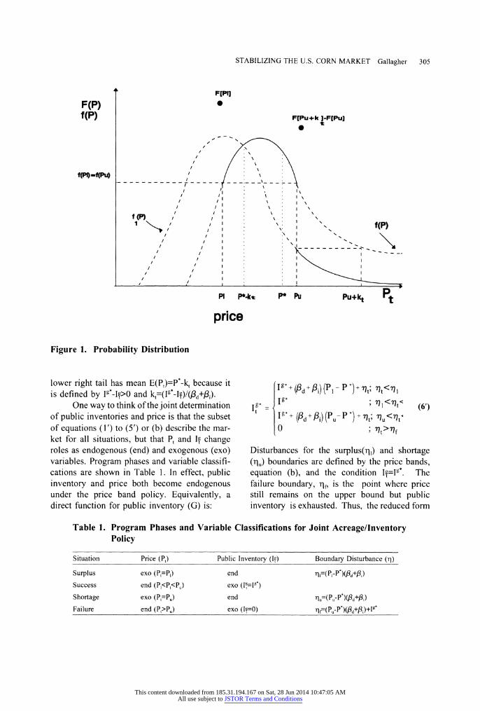
I-=Ig*. However, the probability dis-

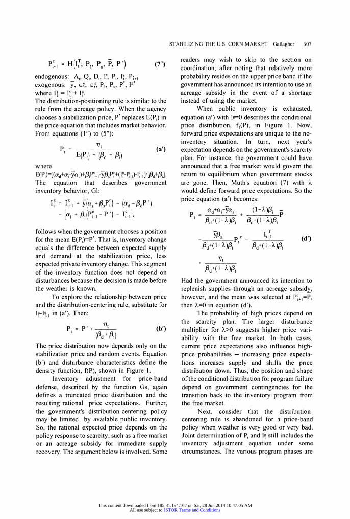
tribution and mean shift downward when actual public inventories are less than the inventory target, Ig*'-I>0. The distribution with the high right tail in Figure I has mean E(P,)=P* because it is defined by I'*-I~=0. The distribution with a

5Variable definitions for policy variables are: P*: stabilization price P1: lower price

Pu: upper price I': public inventory target If: public inventory




F[PI]

F(P) f(P) F[Pu+k ]-F[Pu]

t

f(PI)-f(Pu)

I I

f(P) 1(_) 7 I, f(P)

/ / I

/ / I-

- ---

PI iP*.k

P*Pu Pu+kt Pt

price

Figure 1. Probability Distribution

lower right tail has mean E(P,)=P*-k, because it is defined by 1*-Il>0 and

k,=(Ig*-I_)/(,d+ i). One way to think of the joint determination of public inventories and price is that the subset of equations (1') to (5') or (b) describe the market for all situations, but that Pt and 1I change roles as endogenous (end) and exogenous (exo) variables. Program phases and variable classifications are shown in Table 1. In effect, public inventory and price both become endogenous under the price band policy. Equivalently, a direct function for public inventory (G) is:

Ig'd+ (,d+ i)(P- P )+ 77t; ?t<771

I"* I ; h<qt< (6') Ig*+ (3d+Pi) (Pu-P *)+ 't; OU<'Otu 0 ; 'ot>f

Disturbances for the surplus(r1) and shortage (i,) boundaries are defined by the price bands, equation (b), and the condition 1?=1g*. The failure boundary, 1f, is the point where price still remains on the upper bound but public inventory is exhausted. Thus, the reduced form

Table 1. Program Phases and Variable Classifications for Joint Acreage/Inventory Policy

Situation Price (P,) Public Inventory (If) Boundary Disturbance (rj)

Surplus exo (P,=P,) end rfl=(PI-P')(,Pd+8i) Success end (P,<P,<P,) exo (l=I1')

Shortage exo (P,=Pu) end nu=(Pu-P*)(Ad+fi)

Failure end (P,>Pu)

exo (Ig=0) n=(Pu-P*)(fld+i)+Ig*




equation (6') can summarize government inventory behavior under a price band policy.

The price distribution that includes acreage and public inventory adjustment is crucial for price expectations under the government policy. The distribution is truncated and discontinuous (Figure 1). Let f(P) and F(P) be density and probability functions of the distribution defined by equation (b), the condition I=Ilg*, and probability functions for disturbance terms. This distribution defines price probabilities under success, PJ<Pt<Pu,ll9=I*. Also, the lower tail of this distribution is concentrated on P, because of inventory purchases, giving the chance of surplus F(P1). Now suppose all public inventory is sold: Ip=0. Then, the distribution shifts downward from the position that was occupied when the inventory target was held. This shift is k,=Ig*/(8d+ s).

A piece of this lower distribution describes the probability of program failure, P,>P, and Ip=0O. Finally, part of the high tail of the high distribution is compressed on P, because of inventory sale, giving the probability of a shortage F[P,+kt]-F[P,].

The mean of the truncated distribution is the mathematical expectation of prices under the program:

E(Pt)= PF(P,) + Ep, (P)

+Pu[F(Pu +kt) - F(Pu) (c)

+ EP0 k t P-kt]

where: Pz P=P

EP1[g(P)] = PP I g(P) f(P)dP.

The right-hand-side terms reflect each situation. The first and third terms show concentrated probability at the price bands in surplus and shortage, the second term reflects the distribution f(P) in success, and the fourth term shows reduced probability of extremely high prices in failure.

The expected price depends only on policy instruments, E(P)=H(P,,P,,lg*). Thus, subjective price expectations are straightforward when agents correctly assess the odds and price consequences of program situations. The rational

expected price when the agency keeps the same price band and inventory target is the mean of the truncated distribution. So, equation (7') can be added to equations (I') to (5') for endogenous price expectations and a usable simulation system.

Inventory Management Now consider the details of a program

based on inventory management. For the planting period, the government still chooses a stabilization price, P*, that should occur when there is normal weather. A public inventory rule is based on the desired utilization and the stabilization price; the rule is given below. For the post-harvest period, the agency occasionally abandons its planting period inventory position; it will buy additional inventory to protect a price floor, P,, and it will sell additional inventory to defend a price ceiling, P,. The government's inventory behavior in this hypothetical policy is completely specified. This hypothetical policy is assumed to be announced to the public.

Now producers control acreage decisions and respond to price expectations (equation (1 ")). Other conventional market relationships, given by equations (2") to (5"), remain the same. The government usually positions the price distribution by taking its inventory position before weather is known (equation (6"), Gl), but occasionally defends price bands through inventory positions after harvest (Gs). Now expectations reflect interactions among anticipations, prices, and inventory decisions (equation (7")).

At= as + sPt (1")

t t +eA (2")

Dt = ad - PdPt + Et (3")

I= ai i+ (pel- Pt) (4")

t + + Q= + (5")

I =GIP ,I , P1 , PP or

GS( e T ) (6")

Pt+l; I t, Pz Pu, pt, t E, t




Pt t ' H(I'; P,, Pu, P, P) (7")

endogenous: A,, Q,, D,, ID, Pt, I0, Pl, exogenous: y, ey, e'T, p P,, P *, P

*, 1

where IT = I + Ig The distribution-positioning rule is similar to the rule from the acreage policy. When the agency chooses a stabilization price, P* replaces E(Pt) in the price equation that includes market behavior. From equations (1") to (5"):

Pt=t (at)

E(Pt) + (Id+ (ai) where

E(P)-[(ad+a,-yas)+PiP't+l-yPsPlt+(19-lg The equation that describes government inventory behavior, Gl:

It - t , + (a + f3P) - (ad

-fdP *) -[a +

i( p* I - Ic

follows when the government chooses a position for the mean E(P,)=P*. That is, inventory change equals the difference between expected supply and demand at the stabilization price, less expected private inventory change. This segment of the inventory function does not depend on disturbances because the decision is made before the weather is known.

To explore the relationship between price and the distribution-centering rule, substitute for

I-I_, in (a'). Then:

Pt = P* + 77

(b') (Pd + i) The price distribution now depends only on the stabilization price and random events. Equation (b') and disturbance characteristics define the density function, f(P), shown in Figure 1.

Inventory adjustment for price-band defense, described by the function Gs, again defines a truncated price distribution and the resulting rational price expectations. Further, the government's distribution-centering policy may be limited by available public inventory. So, the rational expected price depends on the policy response to scarcity, such as a free market or an acreage subsidy for immediate supply recovery. The argument below is involved. Some

readers may wish to skip to the section on coordination, after noting that relatively more probability resides on the upper price band if the government has announced its intention to use an acreage subsidy in the event of a shortage instead of using the market.

When public inventory is exhausted, equation (a') with I=0 describes the conditional price distribution, f,(P), in Figure 1. Now, forward price expectations are unique to the no- inventory situation. In turn, next year's expectation depends on the government's scarcity plan. For instance, the government could have announced that a free market would govern the return to equilibrium when government stocks are gone. Then, Muth's equation (7) with k would define forward price expectations. So the price equation (a') becomes:

P ad+ayi-Yas+ (1 t / + - +

d+(1 )i P

T

Y3s te t1 (d')

3d+(1-3i)P -

13d+(1-

X)3i 77t

3d+(1-)348 Had the government announced its intention to replenish supplies through an acreage subsidy, however, and the mean was selected at P1 ,=P, then X=0 in equation (d').

The probability of high prices depend on the scarcity plan. The larger disturbance multiplier for >0O suggests higher price variability with the free market. In both cases, current price expectations also influence high- price probabilities - increasing price expectations increases supply and shifts the price distribution down. Thus, the position and shape of the conditional distribution for program failure depend on government contingencies for the transition back to the inventory program from the free market.

Next, consider that the distribution- centering rule is abandoned for a price-band policy when weather is very good or very bad. Joint determination of P, and I still includes the inventory adjustment equation under some circumstances. The various program phases are




Table 2. Program Phases and Variable Classifications for Inventory Policy

Situation Price (P) Inventory (If) Equations Boundary Disturbance (r1)

Surplus exo (P,=P,) end ( 1 ")-(5") ri=(P,-P )(P+p/3) Success end (P,<P,<P,) end (")-(6",G) Shortage exo (P,=Pu) end (1")-(5") qu =(Pu-P*)(fd+ii) Failure end

(P,>Pu) exo(lI=0) (1")-(5") rl[=y [a,+sP-[a-fdPu]

_-[a_+_( 1-4)(-I Pu)-IL, -If.,

shown in Table 2. Disturbances for the surplus and shortage boundaries, r9, and rlu, are defined by the price band and equation (b'). The failure disturbance, rq, gives Pu

in equation (d') just as the inventory is exhausted (I=0). A direct inventory function that reflects band defense, Gs, is obtained by solving equations (1") to (5") for public inventory. A direct inventory function that reflects all program phases is shown in equation (6") below. Equation (6") describes government inventory during adjustments between distribution-centering and band defense. Public inventory does not depend on the disturbance when the price falls within the band. Other- wise, the disturbance does influence public inventory.

The mean of the truncated price distribution is still described by equation (c); however, probability concentration on the upper band deserves attention. The lower bound of the appropriate interval, Pu, corresponds to the disturbance, qu.

The upper bound corresponds to the disturbance rq, that just exhausts the inventory at Pu

- the corresponding price is

Pt=P*+rl[/(Pd+3i). Probability concentration on the upper band is defined on F(P) by Pu<Pt<P{.

So the range of price events that is compressed on the upper band is k,=Pf-P,. Further substitu- tion with expressions for boundary disturbances gives:

kt t (e') tpd+Pi)

where:

I assP - (ad-3dP ) - [a i(Pe,-P )

t-1 , t+1=P(1-X) + XP.

If is the boundary public inventory when private storage operators buy at P* and expect a market regression from Pu. Alternatively, an acreage policy is expected when ;=0O and operators expect the equilibrium price in the subsequent period. Thus, probability concentration on Pu depends on the plan for the transition back from the unregulated market. More probability resides on the upper band when X=0 because P,+, is lower and It is higher. Increasing current price expectations also raises current supply, the boundary inventory, and the chance of the upper band with either transition plan.

I +

Y s

+-

Ps

ea(a

d d i p tct

Pt-I P?( P d-fgdP*) - [

+Iai+Pt--P*) t--I ;

71<rit<riu 1e 19 p _pf (6") I = Il +yYa+P)

-

(d-dPu) - [u ii(Pte-P) - I + 6t

)t1u t 0 ;ot> t




The expected price that reflects the odds and price consequences of each program situation depends on policy instruments, subjective expectations, and beginning inventory:

E(Pt)= h[Pe, it; T1, P, Pu, P P*

The function, h, is defined by the probability function F(P), the mean of the truncated distribution equation (c), the price distribution that describes program failure equation (d'), and the extent of price-compression onto Pu by the inventory program equation (e'). On balance, an increase in Pc most likely lowers the mean price because high-price probability is transferred to the lower value, Pu, from the upper tail. The interaction between perceptions and the truncated mean is taken into account when agents correctly evaluate all situations. The rational expected price is evaluated numerically by choosing various values of PR until E(P,)=P . So, equation (7") can be included in a usable simulation system. The function H defines the rational expected price from the function h and the condition E(P,)=Pc. The time index can be shifted forward because agents know the form and extent of upcoming government interventions.

Coordination

Harmonious adjustment among program phases and market forces should define policy instrument choices. A coordinated program has a distribution-centering price, P, that is consistent with the price bands, P,,Pu; a band width, d=Pu-P,,

that is wide enough to guarantee reliance on centering policy; and a level for the price structure that excludes producer support.

P* positions the untruncated distribution. Then, a low (high) band increases the chance of emergency inventory sale (purchase) in defense of the upper (lower) band. The highest probability of obtaining an outcome within a band of given width, or the highest success probability, requires band positioning with density function values that are equal at interval endpoints, f(P,)=f(Pu). Otherwise, the chance of obtaining an observation within the interval can be increased by moving the band toward the point with the low density function value. The intersection of a horizontal line and the density

function should define a price band when P' positions the distribution in Figure 1.

The width of the price band defines the frequency of distribution-centering management. Very wide bands almost always exclude short- run inventory adjustment. In contrast, the limiting narrow band almost always excludes distribution-centering and delivers a fixed postharvest price through inventory adjustment. Band widths should imply reliance on distribution-centering, with occasional inventory adjustment.

Simulations that exclude producer support are developed by restricting the average price over a number of outcomes for the managed market to equal the long-run equilibrium price of the free market. A policy-price structure that satisfies this requirement for the acreage- inventory policy can be found without difficulty because the mean of the truncated distribution (equation (c)) also defines the unconditional mean of prices. Thus, the price structure, (P,, P Pu), can be adjusted until E(P,)= P for a simulation with the average price equal to the market's long-run equilibrium.6

For inventory programs, the distribution- centering price, P*, is set equal to the long-run market equilibrium for a first approximation to programs that exclude producer support. This requirement is sensible because it is a condition for equilibrium in public inventory adjustment.' Thus, when the market is near the free market

"Also, increases in IP9 transfer probability from the high tail to the upper band when P,, P', and

Pu are given.

Then, the mean of the truncated distribution and the average of market prices over a large number of observations falls towards P. So, a high (low) stabilization price will yield a high (low) inventory target and a low (high) failure probability in a stabilization program that excludes price support. Policy makers can choose from P" and I`g pairs for a desired chance of failure.

7To see this, notice that P +,=P=P_=P,=P

defines a long-run equilibrium of the market. Then, the inventory change is:

It t I= y(as +,P)- (a-PdP')

-api(P-P)I - Iti

The public inventory change is zero when it is also true that P'=P because the private inventory change is zero, and by definition, supply equals demand at equilibrium.




equilibrium, government stock accumulation is excluded.

However, excluding price support in the sense defined above may not exclude producer income support. Sometimes, simulations that exclude price support yield producer incomes above free market levels. Then, P' is adjusted in a few simulations so that average prices fall below P.

A coordinated policy is a candidate for inclusion in a law if the welfare consequences are favorable compared with the unregulated market. Theoretical literature does suggest difficulty in developing welfare-maximizing rules and instrument choices that remove incentives for revision by future policymakers (Kydland and Prescott; Calvo; Sargent). Nonetheless, the law could be consistent with the recommendation that program rules be known and not changed (Lucas). These programs also include explicit contingencies for the transition between market and government during acute shortage and surplus, which could mitigate the temptation for revision by future policymakers.

Welfare and Public Expenditure Measures

The welfare evaluation in this article is based on surplus measures and identities that define public revenue and expenditure. Consumer surplus approximates willingness to pay (Willig). Producer surplus measures the excess of returns over variable costs in general. Surplus for agricultural production must also account for both uncertainty and government programs. Surplus analysis for inventories accounts for uncertainty and the unique benefits associated with convenience yield.

Consumer Surplus The demand equation (3) may be used to

define consumer surplus as the triangle below the demand curve and above the price line with area:

JId 1)\d tD.

Producer Surplus Total variable costs are determined when

planting occurs, before the price or growing conditions are observed. Costs are given by the area under the expected output schedule (Just, Hueth, and Schmitz). The acreage and production equations, (1) and (2), lead to an expected output schedule of

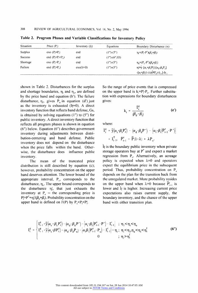
EQs-y (as+PFsP). Profit-minded producers with given expected returns per unit output (P ) choose expected output (y5At) as defined by this supply schedule (Figure 2). An elastic segment of the supply schedule, which corresponds to a break-even price for the most efficient producers, b, adjusts producer surplus to actual levels.' Total variable cost is area C in Figure 2.

On the revenue side, producers respond to government incentives and market prices. A voluntary program is assumed for achieving the targets of the acreage/inventory policy. A payment, d, is offered on the desired reduction of planned production to EQs in Figure 2. Similarly, a subsidy, d,<O, is offered on the desired output expansion to EQs. Together, the acreage target, expected market price, and planned production schedule define the required diversion or subsidy payment:

d e p

At-as dt = s

The producers receive the diversion payment rate multiplied by the amount that production is reduced. Then payments are given by area D for a production decrease and by area S for a production increase. Producer revenue from the acreage program is:

C yd

= d 2.(as+sPs)

- _ as+ P ed

= sd2

8A surplus value that is 20 percent less than corn returns over variable costs during the 1983 to 1987 period (7,500 million dollars) approximates the equilibrium when government programs are eliminated. The estimate, b=$1.395/bu satisfies this condition. Simulations were not affected by the kink in the supply schedule because the expected price always defined a point on the upward-sloping segment of the supply curve.




expected price

Supply p-p d d < 0

ttt t-----

P"P t t

I

Iexpected output

Ea EO=myA EQ I t 2

Figure 2. Producer Cost and Subsidy

Producer surplus is the sum of market and government payments to producers less variable costs:

ts Pt qt+

Ysd2

i( - (ast+sb) (Pe-d-b) + b5At Private Inventory Surplus

The net carrying costs associated with inventories include direct storage costs (interest, loading, and spoilage) minus convenience yield. Profit-minded agents choose inventory storage that balances the storage price, Pe-Pt-,, and the marginal net carrying cost in Figure 3. Variable costs are the area below the net marginal cost schedule and above the horizontal axis (B in Figure 3). Similarly, the area above the net marginal cost schedule and below the

horizontal axis gives convenience yield (A). Thus, the net cost is B-A.

Consider inventory marginal cost, equation (4), for an inventory surplus measure. The storage decision, Il_,, and variable costs were set in the preplanting period. The price was P,-, and the expected price for the postharvest period was Pe. Net variable costs from the preplanting period are given in the second term of the surplus expression. Postharvest revenues are obtained when speculators sell last year's storage, I_, , and buy inventory to hold for next year, Ic, at the postharvest price, Pt. The net gain from actual postharvest revenues and preplanting expenses is:

II = P I- IC C e

P




Supply price b t

b-P -P t t t-1

B SII

-, prrivate A Inventory /C

Figure 3. Inventory Net Cost

Government Expenditures and Revenues

The cost of the public inventory operation is:

C t= Pt(I- i1)+ cl,.

In subsequent simulations, it is assumed that annual grain storage payments under recent Farmer-Owned Reserve programs, $0.265/bu, are the constant storage cost of publicly-held grain (Burnstein and Langley). Total public expenditures can also include the acreage program that has been described.

Simulation

An unregulated market for the U.S. corn industry is compared to a regulated industry that includes government-operating supply adjustment rules. This comparison is based on simulations of the market-government models with random drawings of yield and demand

disturbances. Attention to the corn industry is required, including market structure and the characteristics of random yield and demand disturbances. The specifics of coordinated programs also rely on market and random structure. Finally, the initial conditions of simulations all use the long-run equilibrium of the unregulated market, thereby assuming that the government will not begin stabilization during unusual periods.9

9As a general principle, statistical estimation and validation of government behavior should be included with the simulations; however, estimations could give unstable parameter estimates because the government has not consistently pursued one policy strategy during the last 20 years. Further, the government behavior developed in this report is consistent with reality inasmuch as inventory targets and set-aside adjustment rules are taken into account. But, a law change toward less discretion and more disclosure in setting supply adjustment rules would be required before the government behavior described in this report could occur.




Corn Market

Estimates of U.S. corn market relationships are obtained from other studies and some independent estimation. The demand function slope reflects adjustments in livestock, feed, processing, and export (Westhoff et al.). Esti- mates for yield levels, adjustments, and random effects are taken from Gallagher.

Private inventory response was estimated with data from the United States Department of Agriculture (USDA), the Chicago Board of Trade (CBT), and the International Monetary Fund (IMF). Private inventories were found to depend on expected returns, interest costs and storage capacity. The Ordinary Least Squares (OLS) result below uses data from 1970 to 1989:

It = 349.56 780.87nb, + .340

cr (1.25) (3.08) (4.78) R =.672 s = 298.7 D.W. = 1.44

IC: Off-farm storage on December 1, year t, mill bu (United States Department of Agriculture)

nbt: net storage return, $/bu, nb,=Pf~'+-Pft-rtPft

Pf+"': December futures, delivered in year t+1, quoted in year t, $/bu, (CBT)

rt: treasury bill rate, fourth quarter (IMF) c,: off-farm storage capacity at 10 states,

mill bu (United States Department of Agriculture): (Illinois, Indiana, Iowa, Michigan, Minnesota, Missouri, Nebras- ka, Ohio, South Dakota, Wisconsin).

The simulation equation uses 1989 data and interprets the futures price to be the expected price:

It = 1994.58 + 780.87(Pte+1-Pt)

Models with nonlinear price responses were considered, without improving the fit.

Levels for all functions were adjusted to satisfy the trend level of demand in 1989: 7,800 million bushels. The corresponding trend (mean) yield was 100 bu/planted acre. As a first approximation, it was assumed that the long-run equilibrium area was 78.0 million acres with the corresponding price of $2.40/bu. Market schedules that satisfied these conditions were:

as = 62.4 ad = 9576.0 a, = 1994.6

Ps = 6.5 Pd = 740.0 Pi = 780.9

Linear market relationships are credible, according to the inventory response estimate and the demand function estimates reported by Westhoff et al.

Stochastic simulations were based on a 500 observation sample drawn from a random number generator. Yield disturbances were obtained from estimates of a skewed distribution.'o The standard deviation about a trend line of the 1970's and 1980's demand defined an independent normal distribution for the demand disturbance - the standard deviation estimate was 559.5 million bushels.

The disturbance sample was obtained from combined yield and demand disturbances. First, thresholds in the disturbance population were identified for I-in-50-year events, 1-in- 100- year events, and 1-in-200-year events because there was still some sampling variation in estimates for the tail of the distribution in a sample of 500 observations. Then, several samples were drawn by computer until sample behavior in the tails approximated the corresponding population values. The observations for yield and demand disturbances were also expressed as deviations about mean values.

Policy Characteristics

The policy instrument values chosen for these simulations are shown in the top rows of Tables 3 and 4. These policy prices and inventory targets conform to the criteria for coordinated policies.

1oThe inverted probability function for the Weibull distribution has a convenient form:

x = exp In [-2021n(1- [(2a) Values on a Weibull distribution are transformed values of a random sample for 4 on [0,1]. The maximum likelihood estimates of parameter values are a=.6334 and 0=3.1236. The distribution has a mean of 9.69 and a standard deviation of 7.7 bu/acre. Random values were also multiplied by 1.6946, reflecting secular standard deviation increases and 1989 conditions. The scaled standard deviation is 13.05 bu/acre.



Table 3. Simulation Resultsa

Inventory, Switching to: Free Policy Acreage Policy Free Market Joint Acreage and Inventory Market

Band Width (d) ($/bu) units 1.75 0.75 1.75 2.15b 0.75 1.75 none

Probability Surplus 0-1 .050 .200 .050 .032 .200 .050 -- Success 0-1 .792 .427 .792 .870 .427 .792 -- Shortage 0-1 .012 .024 .000 .000 .316 .097 -- Failure 0-1 .145 .347 .157 .098 .056 .061 --

Policy Instrument Lower Price (Pl) $/bu 1.4475 1.775 1.375 1.270 1.935 1.425 Upper Price (P) $/bu 3.1975 2.525 3.125 3.420 2.685 3.175 Stabilization Price (P') $/bu 2.4725 2.400 2.400 2.395 2.560 2.450 Public Inventory Target (I') mil bu 100.02 100.02 100.02 5.0 1,885.6 942.9 --

Market and Endogenous Policy Area Planted (At) mil acre 78.15 77.97 78.04 78.00 77.92 78.00 78.00

(1.25) (1.33) (1.11) (5.73) (8.69) (6.80) (1.62) Production (Q) mil bu 7,817.20 7,799.90 7,806.20 7,802.30 7,794.30 7,802.90 7,802.00

(971.00) (968.00) (966.00) (1,123.00) (1,305.00) (1,180.00) (972.00) Demand (Dr) mil bu 7,779.000 7,792.90 7,798.50 7,801.10 7,793.10 7,801.80 7,801.20

(483.00) (561.00) (540.00) (543.90) (470.50) (496.00) (615.60) Price (P) $/bu 2.401 2.409 2.402 2.398 2.409 2.397 2.398

(0.55) (0.71) (0.701) (0.713) (0.349) (0.591) (0.870) Commercial Inventory (It) mil bu 1,993.300 1,984.300 1,999.70 1,996.01 1,987.50 1,996.70 1,995.70

(426.20) (404.10) (435.00) (556.40) (272.90) (461.00) (486.30) Public Inventory (If) mil bu 3,167.600 518.40 666.10 12.30 1,659.30 865.50 0

(2,169.00) (872.60) (934.00) (65.40) (645.40) (271.00) Diversion/Subsidy Payment

(dt) $/bu -0.023 -- - 0.001 0.013 -0.006 0

(0.19) -- -- (0.881) (1.340) (1.037)

"Mean values with standard deviations in parentheses.

bHighest net welfare.

"Initial value.

C)I m

ril

0

H

<

Cd

0

ON

z

0

7tc

r-

m

oC

0\ oj

O



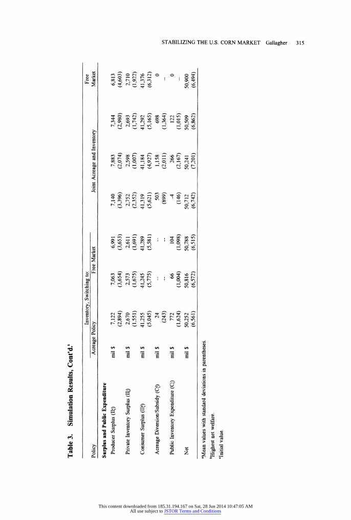
Table 3. Simulation Results, Cont'd.a

Inventory, Switching to: Free Policy Acreage Policy Free Market Joint Acreage and Inventory Market

Surplus and Public Expenditure Producer Surplus (II) mil $ 7,122 7,063 6,991 7,140 7,883 7,344 6,813

(2,894) (3,654) (3,653) (3,396) (2,074) (2,980) (4,603) Private Inventory Surplus (IID mil $ 2,670 2,573 2,611 2,752 2,598 2,693 2,710

(1,551) (1,675) (1,691) (2,352) (1,007) (1,742) (1,922) Consumer Surplus (IId) mil $ 41,255 41,245 41,289 41,319 41,184 41,292 41,376

(5,045) (5,775) (5,581) (5,621) (4,927) (5,165) (6,312) Acreage Diversion/Subsidy (Cd) mil $ 24 -- - 503 1,158 698 0

(243) -- -- (899) (2,011) (1,364) Public Inventory Expenditure (Ci) mil $ 772 66 104 -4 266 122 0

(1,624) (1,004) (1,098) (146) (2,167) (1,015) Net mil $ 50,252 50,816 50,788 50,712 50,241 50,509 50,900

(6,561) (6,572) (6,515) (6,742) (7,201) (6,862) (6,494)

*Mean values with standard deviations in parentheses. bHighest net welfare.

"Initial value.

Cd)

H

Cd

rcl H




Table 4. Simulation Results with Reduced Average Market Pricesa

Inventory, Switching to Joint Acreage

Policy Acreage Policy and Inventory

Band Width (d) ($/bu) units 1.75 1.75

Probability Surplus 0-1 0.050 0.050 Success 0-1 0.792 0.792 Shortage 0-1 0.012 0.097 Failure 0-I 0.145 0.061

Policy Instrument Lower Price (P,) $/bu 1.375 1.375 Upper Price (P.) $/bu 3.125 3.125 Stabilization Price (P*) $/bu 2.400 2.400 Initial Public Inventory or Target ([') mil bu 100.000 942.900

Market and Endogenous Policy Area Planted (A,) mil acre 78.410 78.380

(2.680) (6.770) Production (Q,) mil bu 7,844.700 7,840.200

(1,010.000) (1,185.620) Demand (D,) mil bu 7,836.600 7,838.900

(498.000) (497.100) Price (P) $/bu 2.350 2.347

(0.590) (0.593) Commercial Inventory (I1) mil bu 2,001.200 2,035.900

(450.500) (462.700) Public Inventory (If) mil bu 1,096.000 865.167

(1,027.000) (272.000)

Diversion/Subsidy Payment (d,) $/bu -0.102 -0.058 (0.400) (1.042)

Surplus and Public Expenditure Producer Surplus (II) mil $ 6,775 6,949

(3,045) (3,020) Private Inventory Surplus (IIt) 2,680 2,693

(1,685) (1,702) Consumer Surplus (IId) mil $ 41,664 41,686

(5,209) (5,204)

Acreage Diversion/Subsidy (Cd) mil $ 111 705 (561) (1,420)

Public Inventory Expenditure (Ci) mil $ 208 121 (1,324) (1,001)

Net mil $ 50,801 50,501 (6,533) (6,879)

aThe mean values with standard deviations are in parentheses.




Price bands are defined by the high chance of success criterion for coordinated policies."' Simulations for the acreage/inventory and the inventory policy both consider moderate and wide bands, $0.75/bu and $1.75/bu. The moderate and wide bands have success probabilities of 0.4 and 0.8, respectively. A wider band of $2.15/bu is also included in the acreage policy because it has the highest net welfare.

The overall price structures, (P,,P* P,), give average prices that are near free market equilibrium. The solutions in Table 3 all have an average market price that equals the free market equilibrium of $2.40/bu. In the acreage/ inventory programs with moderate and wide bands, the high stabilization price, P, and high inventory target, Ip' are consistent with the low failure probability of 0.06. P* and Ig" are lower with the widest band. For the inventory programs, P* was set at P , except when the acreage subsidy was used during scarcity.

A similar set of simulations (Table 4) both feature a wide band and lower price structure. The average price, $2.35/bu, reduces average producer income to the free market level.

Results

The market outcomes and welfare indicators for simulation experiments are given in Tables 3 and 4. The columns contain results for inventory programs, acreage/inventory programs, and the free market, respectively.

In Table 3, the right-hand columns summarize experiments with narrow (0.75) and

wide (1.75) bands for the acreage/inventory policies. Net welfare increases as the band widens and inventory target decreases. In contrast, reductions in price and farm income instability and increasing farm income are associated with band narrowing. Specifically, average producer surplus is 15 percent greater and the variability of price and farm income is 60 percent less with the narrowest band policy, compared with the unregulated market. Also, on average, storage operators lose annual income (4 percent), but gain more stable income.

The left column for the acreage/inventory policy summarizes the results of a grid search that was designed to find the greatest net welfare. This search started with nine policies defined by alternative price bands and inventory targets. The reported result has the highest net welfare from simulations with alternative inventory targets and band widths. The net welfare level is close to the free-market solution (50.7 versus 50.9 billion dollars). This corner solution features a public inventory target that is about zero. The public cost decreases associated with excluding public inventory and less variable acreage that omits adjustments for public inventory may be reasons for these results.

Inventory results are shown in the left-hand columns of Table 3. The case where free markets emerge during scarcity and the case of occasional acreage subsidies during scarcity are both included. Price and farm income instability is still reduced and farm income is still improved in comparison to the unregulated market. How- ever, most changes are moderate. In particular, farm price and income variability are about 20 percent less under the inventory/ market program than in the free market. Also, small net welfare reductions are about 0.1 billion dollars less than the free market. The net welfare change includes gains to producers and losses for consumers, taxpayers, and inventory speculators. The mag- nitudes range between 2.5 and 5.0 percent. The inventory program with occasional acreage subsidies shows a similar pattern of stability and benefit changes. However, speculator losses are small. Also, the instability reduction is large. Notice that average farm income consistently increases in comparison to the free market.

"A histogram for f(P), obtained from a computer- generated sample, was based on the disturbance from equations (b) and (b'):

r7t (1d +fi)

where q=CE-AYd . A 10,000 observation sample for corn yield and

demand disturbances was constructed from probability function estimates. These estimates were combined with the corn market response estimates, p/ and ,/, for a frequency distribution of price deviations. As a first approximation, area was held at the long-run equilibrium value: A,=78 mil acres. Next, a positive deviation and a negative deviation that have equal density function values were added to a given stabilization price for both a lower band and an upper band.




Accordingly, programs with reduced income support deserve attention.

Two programs with lower price structures and wide bands are shown in Table 4. Both programs still reduce price and income instability. But, on average, farm income is lower and comparable to the free market level. Further, consumer welfare is higher than in the unregulated market. In the acreage program, there is no net welfare gain from reducing the price level because program expenditures are also increased. However, the inventory-subsidy program is suited to the lower price structure, because there is a net welfare gain associated with reduced expenditures on the public inventory program.

Summary and Conclusions

This article considers plausible price stabilization programs that are relevant to U.S. grain markets. The markets are characterized by unstable supply and demand, an efficient storage industry, and economic agents with rational expectations. The government takes market behavior into account and knows the long-run market equilibrium. The government acts before weather and demand conditions are known, setting the mean of the price distribution near the equilibrium price of the unregulated market. The government occasionally acts after weather and demand conditions are known, defending the lower (upper) price of a band through inventory purchase (sale). Alternative programs include joint acreage and inventory management, inventory management with free market policy during scarcity, and inventory management with an occasional acreage subsidy during scarcity.

A simulation study, based on the structure of the U.S. corn market, suggests that government policies can stabilize prices and farm incomes. A moderate stability improvement occurs for the inventory program that allows markets to emerge during scarcity. Substantial improvements occur under the combined acreage/inventory program with a narrow band and the inventory/subsidy program. Furthermore, coordinated programs that exclude price support consistently improve farm income, as producers gain more from avoiding low prices than they lose as access to high prices in an inelastic

market. The farm income increase is high in the acreage/inventory program or the inventory/ subsidy program, and moderate in the inventory/ market program or the acreage program that excludes inventory. Consumer losses, speculator losses, and public expenditures are roughly proportional to producer gains. Of the programs that exclude producer income support and favor consumers, the inventory/subsidy program has the most favorable net welfare evaluation.

The most efficient programs are the acreage program that excludes inventory and the inventory/subsidy program without producer income support. These programs have net welfare levels that are close to the unregulated market. Perhaps the government should avoid joint management of acreage and inventories, unless there are exceptional circumstances.

These results lend credibility to arguments for stabilization that are based on intangible benefits such as risk reduction for producers and storage operators or food security for consumers. But the argument also hinges on an adept public agency that knows and acts on private sector behavior, the market's long-run equilibrium, and the range of random shocks to the market. Finally, efficiency requires that market agents know government supply-adjust-ment rules. Maybe market performance could be improved with more explicit stabilization rules and more complete disclosures of government behavior.

[Received February 1993. Final version received January 1994.]

References

Burnstein, H. and J. Langley. "A Description of U.S. Grain Reserve Programs." The Farmer-Owned Reserve qfter Eight Years: A Summary of" Research Findings and Implications, ed. W.H. Meyers. Iowa State University Agriculture Experiment Station Research Bulletin 598, Ames, IA, 1988.

Calvo, G.A. "On the Time Consistency of Optimal Policy in a Monetary Economy." Econometrica 46(1978): 1411- 28.

Chicago Board of Trade. Statistical Annual 1984. Chicago, 1984.

Gallagher, P. "U.S. Corn Yield Capacity and Probability: Estimation and Forecasting with Nonsymmetric




Disturbances." North Central Journal of Agricultural Economics 8(1986):109-22.

Gardner, B.L. Optimal Stockpiling qf Grain. Lexington, KY: D.C. Heath Company, 1980.

Glauber, J., P. Helmberger, and M. Miranda. "Four Approaches to Commodity Market Stabilization: A Comparative Analysis." American Journal of Agricultural Economics 71(1989):326-37.

Gray, R.W. and A.E. Peck. "The Chicago Wheat Futures Market: Recent Problems in Historical Perspective." Food Research Institute Studies 18(1981):89-1 15.

Helmberger, P. and R. Weaver. "Welfare Implications of Commodity Storage under Uncertainty." American Journal of Agricultural Economics 59(1977):639-51.

Houck, J.P. "Stabilization in Agriculture: An Uncertain Quest." Agricultural Policies in a New Decade, ed. K. Allen, pp. 173-99. Washington, DC: Resources for the Future, 1990.

International Monetary Fund. International Financial Statistics, vol. XXIX, No. 6, June 1976.

Just, R.S., D. Heuth, and A. Schmitz. Applied Welfare Economics and Public Policy. Englewood Cliffs, NJ: Prentice-Hall, 1982.

Kaldor, N. "Speculation and Economic Stability." Review of Economic Studies 8(1939):1-27.

Kydland, F.E. and E.C. Prescott. "Rules Rather than Discretion: The Inconsistency of Optimal Plans." Journal of Political Economics 85(1977):473-91.

Lucas, R.E. "Econometric Policy Evaluation: A Critique." The Phillips Curve and Labor Markets, ed. K. Brunner and A. Meltzer, pp. 19-46. Amsterdam: North-Holland, 1976.

Magee, J.F. "Guides to Inventory Policy. II. Problems of Uncertainty." Harvard Business Review 34(1956):103- 16.

Massell, B. "Price Stabilization and Welfare." Quarterly Journal of Economics 83(1969):285-97.

Miranda, M.J. and P.G. Helmberger. "The Effects of Commodity Price Stabilization Programs." American Economic Review 78(1988):46-58.

Muth, J.F. "Rational Expectations and the Theory of Price Movements." Econometrica 29(1961):315-35.

Newberry, D.M. and J.E. Stiglitz. The Theory qf Commodity Price Stabilization. New York: Oxford University Press, 1981.

Oi, W.Y. "The Desirability of Price Instability Under Perfect Competition." Econometrica 29(1961):58-64.

Reutlinger, S. "A Simulation Model for Evaluating Worldwide Buffer Stocks of Wheat." American Journal

of Agricultural Economics 58(1976):1-12.

Sargent, T.J. Macroeconomic Theory. Orlando: Academic Press, 1987.

Thompson, S. "Returns to Storage in Coffee and Cocoa Futures Markets." Journal of Futures Markets 6(1986):546-64.

Thurman, W.W. "Speculative Carryover: An Empirical Examination of the U.S. Refined Copper Market." Rand Journal of Economics 19(1988):420-37.

Tilley, D.S. and S.K. Campbell. "Performance of the Weekly Gulf-Kansas City Hard-Red Winter Wheat Basis." American Journal of Agricultural Economics 70(1988):929-35.

United States Department of Agriculture. Grain Stocks. Washington, DC: National Agricultural Statistics Service, GrLg 11-1 (1-90), January 11, 1990.

Waugh, F. "Does the Consumer Benefit from Price Instability?" Quarterly Journal of Economics 58(1944):602-14.

Westhoff, P., R. Baur, D.L. Stephens, and W.H. Meyers. FAPRI U.S. Crops Model Documentation. Center for Agricultural and Rural Development, CARD Technical Report No. 89-Tr, Iowa State University, Ames, IA, August 1989.

Williams, J.C. and B.D. Wright. Storage and Commodity Markets. New York: Cambridge University Press, 1991.

Willig, R. "Consumer Surplus without Apology." American Economic Review 66(1976):589-97.

Working, H. "The Theory of Price of Storage." American Economic Review 39(1949):1254-62.



stabilizing the u.s. corn market

Documents