stable marriage problem and college admission - citeseer

THESIS ON INFORMATICS AND SYSTEM ENGINEERING C27

Stable Marriage Problem and College Admission

TARMO VESKIOJA

Faculty of Information Technology

Department of Informatics

TALLINN UNIVERSITY OF TECHNOLOGY

Dissertation was accepted for the commencement of the degree of Doctor of Philosophy in Engineering on December 9, 2005. Supervisor: Prof. Emer. Leo Võhandu, Faculty of Information Technology Opponents: Prof Dr Mati Tombak, University of Tartu, Estonia

Teaching Researcher D.Sc. Harri Haanpää, Helsinki University of Technology, Finland

Commencement: December 9, 2005 Declaration: Hereby I declare that this doctoral thesis, my original investigation and achievement, submitted for the doctoral degree at Tallinn University of Technology has not been submitted for any degree or examination. / Tarmo Veskioja / Copyright Tarmo Veskioja 2005 ISSN 1406-4731 ISBN 9985-59-583-1

3

Table of Contents

Introduction...................................................................................................... 5

1. The Theory of Stable Marriage Problem............................................ 8

1.1 THE FORMAL MODEL ............................................................................ 8

2. A Development Process of Matching Mechanisms for SAIS .......... 13

2.1 PAST AND PRESENT PROBLEMS........................................................... 13 2.2 THRESHOLD ADMISSION...................................................................... 13 2.3 SAIS ADMISSION SYSTEM AT PRESENT STAGE.................................. 15 2.4 PROPOSED DEVELOPMENT PATH FOR SAIS ....................................... 16 2.5 THE STRUCTURE OF ESTONIAN EDUCATIONAL IS.............................. 17 2.6 STRATEGY-PROOF MATCHING MECHANISM....................................... 18 2.7 MERGE OF SUBMARKETS..................................................................... 20

3. Preference Model ................................................................................ 22

3.1 CONSTRUCTING A PREFERENCE MODEL ............................................. 23 3.2 SORTING APPLICANTS INTO GROUPS .................................................. 27 3.3 ANALYSIS RESULTS ON REAL DATA................................................... 27 3.4 ANALYSIS RESULTS ON STOCHASTICALLY GENERATED DATA.......... 37 3.5 BREAKING OF TIED PREFERENCES ...................................................... 41

4. Majority Voting in Stable Marriage Problem with Couples........... 43

4.1 THE CORE OF A MARRIAGE GAME..................................................... 43 4.2 AN EMPTY CORE EXAMPLE OF MANY-TO-ONE MODEL WITH COUPLES......................................................................................................... 44 4.3 HOW TO SELECT MATCHINGS FOR THE TOURNAMENT...................... 47 4.4 MATCHING FRAMEWORK .................................................................... 47

5. Tournaments as Feedback Set Problems .......................................... 49

5.1 AN ALGORITHM BASED ON A MONOTONE SYSTEM........................... 50 5.2 TOURNAMENT METHOD BASED ON A MONOTONE SYSTEM .............. 50 5.3 THE CONSTRUCTION OF AN EXPERIMENT .......................................... 53 5.4 TESTING RESULTS OF THE TOURNAMENT METHOD ............................. 54 5.5 GLOBAL OPTIMIZATION IN A FAS PROBLEM ...................................... 57 5.6 RESULTS ON LARGE TOURNAMENT TABLES ........................................ 58

Conclusions..................................................................................................... 62

CONCLUDING REMARKS ................................................................................. 62 FUTURE WORK ............................................................................................... 65 AUTHOR`S CONTRIBUTION TO THE PUBLICATIONS........................................ 66 CONTENTS OF THE PUBLICATIONS ................................................................. 66

Kokkuvõte (conclusions in Estonian language)........................................... 71

4

References....................................................................................................... 75

Appendix......................................................................................................... 79

APPENDIX A: THE LOCATION OF ANALYSIS RESULTS .................................... 79 APPENDIX B: CURRICULUM VITAE ................................................................ 80 APPENDIX C: ELULOOKIRJELDUS (CV IN ESTONIAN) .................................... 83

5

Introduction When my supervisor Leo Võhandu suggested 8 years ago to write my

diploma work on a topic named stable marriage problem, I instantly agreed. The topic certainly had an attractive name that seemed to spark interest in almost everybody. The topic is also rich in different variants of the classical problem and it has been studied in many different contexts - economy, game-theory, combinatorics, physics, data structures, algorithm analysis, and many more. It also offers many practical solutions, mainly in the area of entry-level two-sided markets as for example college admissions. The same topic has remained my field of study throughout my diploma work, master thesis and doctoral thesis. The broader aim of this dissertation is to propose a development process of matching mechanisms for the Estonian centralized admission information system SAIS for educational institutions (https://www.sais.ee/index_en.html). Some information system aspects are also discussed. One important stage in the proposed development process is the introduction of a strategy-proof matching mechanism, that is based on a well-known Gale-Shapley algorithm (1962). Without a strategy-proof matching mechanism the participants may choose a strategy to submit false preferences to try to get a better result for themselves. In order to properly evaluate the practical effects of different matching mechanisms there has to be a set of data that consists of true preferences of the participants. A strategy-proof matching mechanism is preferred as a source of such data. At present, there is no admission data in Estonia with such properties.

The second, and more specific aim of this dissertation is to analyze 3 years of admission data of one university to compare the matchings of the current admission system with the matchings of a strategy-proof matching mechanism. As the basis for this analysis a method to construct a preference model for applicants is proposed. Preference model can be used to generate stochastic preferences of applicants. The proposed method transforms applicants' preferences into a voting table, which is transformed into an AHP comparison matrix from which weights of study fields are computed. The results of limiting the allowed number of preferences are given, based on the preference models of the year 2001. Different methods are described to break ties in preferences.

The third part of the thesis considers stable marriage problem with couples - where paired preferences are allowed over two participants on one side of the market. The current centralized matching market in Estonia may evolve to include this property. In the many-to-one (or one-to-one) matching model with couples, the set of stable matchings and consequently the core of the matching game may be empty (Roth and Sotomayor, 1990, theorem 5.11, page 141). Feedback set problems are known to suite well for that situation - the best matching is chosen using submitted preferences in a voting tournament, where finding the best matching is equivalent to solving a minimum feedback arc set problem in a directed unweighted graph. Since this problem is NP-hard, a framework is proposed to guarantee that a good solution is reached in time.

6

A new heuristical method, based on monotone systems (Mullat, 1976), and a possibly new global optimization technique, are proposed for finding a good ranking efficiently. These two methods can be used together or be part of a meta-heuristical method, for example GRASP (as described in Festa, Pardalos and Resende, 2001) that is known to be very good at solving these problems. Some experimental results are given for the proposed methods. R 2.0.1 statistical package (http://www.r-project.org/) was used for factor analysis to test the preference model results. Most of the experiments were carried out using a programming language named J (http://www.jsoftware.com/), that belongs to the APL family of languages. The author of APL as a notation (also called as Iverson notation) and APL and J as programming languages is late Dr. Kenneth Eugene Iverson. The J language was selected because it suits very well to array and matrix operations, the program code is short and concise. The learning curve has been steep for the author of this thesis and it still takes longer than anticipated to implement a simple method in J than in other more traditional languages, but the short code and the possibility to instantly test the code and see the results in J makes it simpler to catch programming bugs. The version of J504b was used for the experiments. The choice of the language was influenced by the needs of experimentation, not by the needs of commercializing implemented algorithms. For real-world implementations it is always possible to recode time-critical functions in some other language (C++, etc.) to try to improve the speed of the programs. The thesis is divided into 6 following sections. The theory of the stable marriage problem and its relevant variants is formulated in paragraph 1.

In paragraph 2 a development process of matching mechanisms for the Estonian central admission system SAIS is formulated, including the proposed strategy-proof matching mechanism. The proposed mechanism is an elaborated version of a mechanism given in the master thesis of Veskioja (2000), some ideas have also been published in Veskioja (2002).

The method to construct a preference model is described in paragraph 3, along with comparative analysis results of the effects of limiting the allowed number of preferences and the description of different methods to break tied preferences. Paragraphs 3.1-3.3 are largely based on the article of Veskioja and Võhandu (2005b). The contents of paragraphs 3.4-3.5 have not been published elsewhere.

Paragraph 4 contains the description of the proposed framework for obtaining a good matching in a limited time when paired preferences are allowed. Paragraph 4 is largely based on two articles of Veskioja and Võhandu (2004a, 2004b).

As part of this framework, the proposed two methods for finding the best tournament ranking is described in paragraph 5 along with experimental results. Contents of paragraphs 5.1-5.4 are partially described in two articles of

7

Veskioja and Võhandu (2004a, 2004b). The contents of paragraphs 5.5-5.6 have not been published elsewhere. Conclusions of the thesis are given after paragraph 5. Conclusions in estonian language follow the conclusions in english language.

Most of the experimental results was decided to be made available in the following address (http://staff.ttu.ee/~tarmov/doktoo/), these results will be revised and updated in the future (while keeping the original versions), if needed. Appendix describes the location and extent of the experimental data in more detail.

This thesis was partially supported by Estonian Science Fund (ESF) Grants

4844, 5918 and G3765. It was also supported in part by EITSA under Grant 04-03-00-27.

I would like to thank my supervisor, prof. emeritus Leo Võhandu, for

guiding me in my path to greater knowledge. To be honest, he started to influence my future even while I was still at high-school - his articles at the magazine "Tehnika ja Tootmine" were one of the main reasons why I chose to study economic data processing at Tallinn Technical University. Leo has always been and still is ready to share any one of his many ideas or interesting books or articles that he has acquired - I owe him many of his books, and many ideas as well. He is great at giving optimism and explaining away hard to understand concepts in a simple manner.

I would also like to thank my superior Rein Kuusik and my colleagues for supporting me in my studies and day-to-day tasks when it was needed. I also thank Indrek Reimand and Indrek Seppo for interesting discussions.

Special thanks will go to my mother Tiia and father Vello for supporting me in my seemingly never-ending studies. I also thank for the moral support of my relatives - there have been (and probably will continue to be) many school teachers and even some principals in our family tree.

As for the obligatory gratitude for the stable marriage partner of the author (see Gusfield and Irving, 1989, or many others), well, what can I say? Instead of saying that "a shoemaker has no shoes" or that "a matchmaker has no match", I will thank her in advance. Donald E. Knuth in his famous book (all his books are famous) "Stable Marriage and Its Relation to Other Combinatorial Problems" (1976, 1997) has formulated 12 open stable marriage problems. The fact, that many of his problems have already been solved, gives me reason to believe that my open problem will also be solved in the not so distant future. In solving this problem, one has to also take into account the different notions and different levels of stability (weak-, strong-, super stability) in a stable marriage (for example, see Gent and Prosser, 2002b).

8

1. The Theory of Stable Marriage Problem Most of the notations, theorems and descriptions of theorems given in this thesis concerning the theory of Stable Marriage Problem originate from the book of Roth and Sotomayor (1990).

2.1 The Formal Model There are two finite and disjoint sets M and W, let them be men and women.

M = {m1, m2, ..., mn} is the set of men. W = { w1, w2, ..., wp} is the set of women. Together they form a set of actors A = M ∪ W. Each man has preferences over the women, and each woman has preferences over the men. That is, a man’s preferences might be of the form P(m1) = w2, [w1, w7], m1, w3, ..., wk indicating that the first choice of the first man m1 is woman w2, as a second choice he is indifferent between women w1 and w7 or in other words he has tied preferences over w1 and w7. Such indifference is denoted by brackets. The third preference m1 shows that man m1 prefers to remain single to marrying anyone else. The same preferences may be shown in a simpler form P(m1) = w2, [w1, w7].

P is the set of preference lists of both men and women P= { P(m1), ..., P(mn), P(w1), ..., P(wp)}. P(M) is the set of preference lists of men M, P(W) is the set of preference lists of women W.

Comparison w > mw’ means that m prefers w to w’, and w ≥ mw’ means that m prefers w at least as well as w’.

Woman w is acceptable to man m if he likes her at least as well as remaining single, that is, if w ≥ m m.

If an actor is not indifferent between any two acceptable alternatives, he or she has strict preferences. The preferences of actors have to be transitive and deterministic to be presented as a preference list.

Transitive preferences mean that if man m likes w1 at least as well as w2 (w1≥m w2) and m likes w2 at least as well as w3 (w2 ≥ m w3), then m has to like w1 at least as well as w3 (w1 ≥ m w3).

The second asssumption is that preferences have to form a complete ordering, this means that any two alternatives can be compared – the actor is never confronted with a choice he is unable to make. When the preferences of an actor form a compete ordering and are transitive, then these actors are called rational. Definition 1.1 A matching µ is a 1:1 correspondence between men M and women W such that if µ(m) ≠ m then µ(m) ∈ W and if µ(w) ≠ w then µ(w) ∈ M (Roth and Sotomayor, 1990, p.19). Matching µ is a set of marriages or a set of pairs, where µ(a) is the mate of actor a. Definition 1.2 The matching µ is individually rational if each actor is acceptable to his or her mate. That is, a matching is individually rational if it is not blocked by any (individual) actor (Roth and Sotomayor, 1990, p. 21).

9

Definition 1.3 A matching µ is stable if it is not blocked by any individual or any pair of actors. That is, a matching is not stable if there exists a man m currently paired with a woman w’, but prefers woman w to w’, and w is paired with m’ but prefers m to m’. Such pair µ(m) = w forms a blocking pair to matching µ.

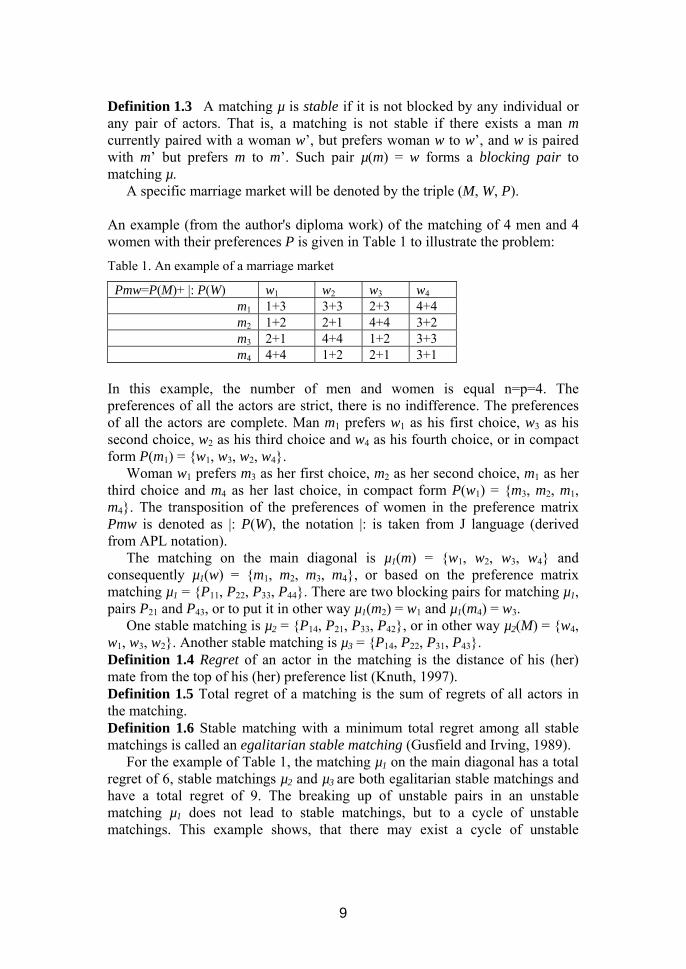
A specific marriage market will be denoted by the triple (M, W, P). An example (from the author's diploma work) of the matching of 4 men and 4 women with their preferences P is given in Table 1 to illustrate the problem: Table 1. An example of a marriage market

Pmw=P(M)+ |: P(W) w1 w2 w3 w4 m1 1+3 3+3 2+3 4+4 m2 1+2 2+1 4+4 3+2 m3 2+1 4+4 1+2 3+3 m4 4+4 1+2 2+1 3+1

In this example, the number of men and women is equal n=p=4. The preferences of all the actors are strict, there is no indifference. The preferences of all the actors are complete. Man m1 prefers w1 as his first choice, w3 as his second choice, w2 as his third choice and w4 as his fourth choice, or in compact form P(m1) = {w1, w3, w2, w4}.

Woman w1 prefers m3 as her first choice, m2 as her second choice, m1 as her third choice and m4 as her last choice, in compact form P(w1) = {m3, m2, m1, m4}. The transposition of the preferences of women in the preference matrix Pmw is denoted as |: P(W), the notation |: is taken from J language (derived from APL notation).

The matching on the main diagonal is µ1(m) = {w1, w2, w3, w4} and consequently µ1(w) = {m1, m2, m3, m4}, or based on the preference matrix matching µ1 = {P11, P22, P33, P44}. There are two blocking pairs for matching µ1, pairs P21 and P43, or to put it in other way µ1(m2) = w1 and µ1(m4) = w3.

One stable matching is µ2 = {P14, P21, P33, P42}, or in other way µ2(M) = {w4, w1, w3, w2}. Another stable matching is µ3 = {P14, P22, P31, P43}. Definition 1.4 Regret of an actor in the matching is the distance of his (her) mate from the top of his (her) preference list (Knuth, 1997). Definition 1.5 Total regret of a matching is the sum of regrets of all actors in the matching. Definition 1.6 Stable matching with a minimum total regret among all stable matchings is called an egalitarian stable matching (Gusfield and Irving, 1989).

For the example of Table 1, the matching µ1 on the main diagonal has a total regret of 6, stable matchings µ2 and µ3 are both egalitarian stable matchings and have a total regret of 9. The breaking up of unstable pairs in an unstable matching µ1 does not lead to stable matchings, but to a cycle of unstable matchings. This example shows, that there may exist a cycle of unstable

10

matchings and that some of the matchings within that cycle can have a smaller total regret than an egalitarian stable matching. Definition 1.7 Matching is a majority assignment (best-voted matching) if there is no other matching that is preferred by a majority (of men and women) to the original matching.

Gärdenfors (1975) observed that, when preferences are strict, the set of majority assignments comprises the set of stable matchings, thus showing that the notion of majority assignment is a relaxation of stability (Klijn and Masso, 2003).

For the example of Table 1, pairwise voting between matchings µ1, µ2 and µ3 is always a draw. Definition 1.8 Weakly stable matching is a matching, which can have a blocking pair which undermines the stability of a matching, but this blocking pair is not credible in the sense that one of the partners may find a more attractive partner with whom he forms another blocking pair for the original matching.

In other words, Klijn and Masso (2003) define an individually rational matching to be weakly stable if every blocking pair is - in the sense above - not credible. Clearly, weak stability is also a relaxation of stability. Theorem 1.9 A stable matching exists for every marriage market (theorem 2.8 in Roth and Sotomayor, 1990, p.27, Gale and Shapley, 1962).

That theorem has been proven using a well-known Gale-Shapley matching algorithm for 1:1 matching markets when the number of actors on both sides is equal (Gale and Shapley, 1962). If both sides are not equal in size, then one can add fictitious actors on the smaller side. For the transformation of different variants of stable marriage problems into the 1:1 formal model see Knuth (1997), Gusfield and Irving (1989) or Roth and Sotomayor (1990). In some of those variants, there can be different levels of stability. For definitions of different levels of stability, see Klijn and Masso (2003) or Gent and Prosser (2002b). Algorithm 1.10 Gale-Shapley algorithm 1. Choose the first free man m from the list of men M. 2. Man m proposes to the first woman w in his preference list, whom m has not

proposed yet. 2.1. If the woman w is not engaged, then she will accept the proposal and m and

w will form a new pair. 2.2. If woman w is already engaged with m', but w prefers m to her current

partner m', then w will break the marriage with m' and form a new pair with m. Man m’ remains single (the first free man in the list of men M).

2.3. If woman w is already engaged with m', and w prefers her current partner m' to the proposing m, then w will reject the proposal (and m will have to keep on proposing to the next women on his preference list).

3. If not all men in M are engaged, then resume with step 1.

11

4. FINISH. That algorithm also has another variant named the deferred acceptance procedure (Roth and Sotomayor, 1990, p. 27-28). Algorithm 1.11 Deferred acceptance algorithm

3. All free men propose to the first woman on their preference list, whom they have not proposed yet.

4. All engaged men will propose again to their current partner. 5. All women that got proposed, will choose the best proposal and accept

that. (Other proposals are rejected and those men have to keep on proposing to the next women on their preference list.)

6. If not all men in M are engaged, then resume with step 1. 7. FINISH.

All men and women are engaged. It has been proved that both of these algorithms have essentially the same

properties, even the same worst-case time and space complexities O(N2). Since in Gale-Shapley algorithm the engaged men do not have to reaffirm their proposal all the time, the average time and space complexity is better than in the deferred acceptance algorithm. Definition 1.12 For a given marriage market (M, W, P), a stable matching µ is M-optimal if every man likes it at least as well as any other stable matching; that is, if for every other stable matching µ', µ ≥ M µ'. Similarly, a stable matching v is W-optimal if every woman likes it at least as well as any other stable matching, that is, if for every other stable matching v', v ≥ W v' (Roth and Sotomayor, 1990, p.32). Theorem 1.13 When all men and woman have strict preferences, there always exists an M-optimal stable matching, and a W-optimal stable matching. Furthermore, the matching µM produced by the deferred acceptance algorithm with men proposing is the M-optimal stable matching. The W-optimal stable matching is the matching µW produced by the algorithm when the women propose (Roth and Sotomayor, 1990, p.32). Theorem 1.14 When all actors have strict preferences, the common preferences of the two sides of the market are opposed on the set of stable matchings: if µ and µ' are stable matchings, then all men like µ at least as well as µ' if and only if all women like µ' at least as well as µ. That is, µ > M µ' if and only if µ' >W µ (Roth and Sotomayor, 1990, p.33). An immediate consequence of this theorem is the following. Corollary 1.15 When all actors have strict preferences, the M-optimal stable matching is the worst stable matching for the women; that is, it matches each

12

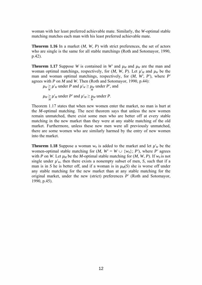
woman with her least preferred achievable mate. Similarly, the W-optimal stable matching matches each man with his least preferred achievable mate. Theorem 1.16 In a market (M, W, P) with strict preferences, the set of actors who are single is the same for all stable matchings (Roth and Sotomayor, 1990, p.42). Theorem 1.17 Suppose W is contained in W' and µM and µW are the man and woman optimal matchings, respectively, for (M, W, P). Let µ'M and µW be the man and woman optimal matchings, respectively, for (M, W', P'), where P' agrees with P on M and W. Then (Roth and Sotomayor, 1990, p.44):

µW ≥ µ'W under P and µ'W ≥ µW under P', and W M

µM ≥ µ'M under P' and µ'M ≥ µM under P. M W

Theorem 1.17 states that when new women enter the market, no man is hurt at the M-optimal matching. The next theorem says that unless the new women remain unmatched, there exist some men who are better off at every stable matching in the new market than they were at any stable matching of the old market. Furthermore, unless these new men were all previously unmatched, there are some women who are similarly harmed by the entry of new women into the market. Theorem 1.18 Suppose a woman w0 is added to the market and let µ'W be the women-optimal stable matching for (M, W' = W ∪ {w0}; P'), where P' agrees with P on W. Let µM be the M-optimal stable matching for (M, W, P). If w0 is not single under µ'W, then there exists a nonempty subset of men, S, such that if a man is in S he is better off, and if a woman is in µM(S) she is worse off under any stable matching for the new market than at any stable matching for the original market, under the new (strict) preferences P' (Roth and Sotomayor, 1990, p.45).

13

2. A Development Process of Matching Mechanisms for SAIS

Financing of higher education in Estonia roughly falls under three categories- the state pays to the universities for about half of the students (so-called RE places), the other half of students are either partially or fully subsidized by the university (TREV places) or the students are fully paying their tuition fees themselves (REV places). Each year the Ministry of Education specifies the number of study places of specialities that are ordered from each higher educational institution (HEI). If not stated otherwise, only bachelor-level studies are discussed in this thesis.

In the past universities and other HEI in Estonia have used its own admission system. Due to that the candidates have had to submit their preferences to several different schools. The existence of many competing sub-markets has caused severe coordination difficulties between these markets.

2.2 Past and Present Problems When the candidate is accepted, (s)he has to decide whether to accept the

offered study place or not. Every school has its own deadline for the candidates. If the candidate declines, then the school has to find a replacement. In essence the problems are very similar to what Roth (1991, 1996) has reported for the NRMP and UK markets.

The competition between Estonian HEI is evident in the numbers of volatility of candidates - about 20-40% of the candidates accepted to one university have also been accepted to other universities and decide that they are better off elsewhere. For some faculties or single study fields these numbers might be much worse - almost all of the originally accepted candidates may choose to go elsewhere, and that can happen even to the most popular study fields with the largest number of free study places. So it is of no surprise, that these study fields have difficulties with finding new candidates, even though a large number of university staff is at work during summertime to try to contact and find new candidates.

As the numbers of students and candidates have soared during the last 10 years, apparently due to the limited workforce the HEI have tried to ease the burden by limiting the number of preferences the candidates can have, to two or three preferences. Even with these restrictions, or because of that, the admission process is still in full swing when the school year begins, which causes frequent changes in the time-table (that itself is an NP-hard task to handle), not to mention the difficulties of those first-year students that have missed their first 2-6 weeks of studies.

2.3 Threshold Admission In the last couple of years, the University of Tartu has gradually introduced a

so-called threshold admission with only one allowed preference in connection with some specialities (study fields). A certain threshold is established to every

14

speciality. Usually, in other Estonian HEI, thresholds ensure the minimum quality of candidates, thereby limiting the list of preferences of schools. In the threshold admission system the purpose of thresholds is to regulate the demand for different specialities. Candidate can choose the speciality if the results of his/her state exams reach the threshold, in such a system the candidate has to submit only one choice.

With the new system the admission staff has much less vacancies to fill, if any at all. But as a result there are no quotas for specialties any more and every year there are some specialities that have to cope with 2-3 times more students than anticipated. The oversupply of students might be good to ensure that enough students graduate the school, especially because the number of government-funded study places is adjusted according to the number of graduated students. The flip-side is that the university has to carry the tuition cost for those candidates that fall outside of the government payed positions - wrong thresholds can turn out to be a substantial burden.

For the university the main problem seems to be the accuracy of predicting the number of students that choose the speciality. Without an accurate prediction it is very difficult to plan ahead the division of resources needed in the teaching process - academic staff, rooms, special equipment, etc.. Many specialities in the University of Tartu do not require special equipment, but for example for an inflated number of medical students one can imagine that there will be a shortage of dead bodies to dissect. If the university is able to accurately predict the demand for speciality then why should it use the threshold system instead of using quotas and, suppose, a candidate-optimal Gale-Shapley matching method? If assuming that the thresholds are exact and the candidates submit their true preferences under a threshold admission system then using the candidate-optimal Gale-Shapley method gives exactly the same result. If the assumptions do not hold, then the Gale-Shapley method gives an even better result.

For students the threshold admission can bring about several strategies that can affect the stability of their true preferences and the stability of matching in respect to their true preferences. Without quotas for specialities it is simplistic to assume that the candidates have enough information to perceive the precise demand of different specialities. Due to that, there will always be specialities with more students than the market requires. To be honest, the same problem plagues other schools as well, because about half of the students pay tuition fees and those who pay are usually not restricted by any quotas. There will be many candidates that prefer popular specialities. There will also be many candidates that prefer a speciality without a prospect of oversupply of workforce - that oversupply might realize as a problem as early as during the admission to masters studies, if masters studies are under a quota. With these seemingly contradictory strategies it is questionable whether the preferences will converge to stable preferences (real or not). That means that if the school does not use quotas to limit the supply, the real preferences of many candidates

15

will depend on the aggregate preferences of others. Without stable real preferences there is no hope for a stable matching of candidates to study places.

The opposing strategies of candidates will make it much more difficult for the university to predict the numbers of candidates that choose a speciality. The prediction is usually based on the admission numbers of previous years. The prediction is based on an assumption that the previous year is a good indicator of choices of candidates (so in the previous year the real preferences found a relatively stable state), that are assumed to be mostly based on speciality thresholds. If one of these assumptions is false, then the prediction will not be accurate and the attempts to correct admission numbers by raising or lowering thresholds will further destabilize the (true and stated) preferences of candidates. Seemingly the only way to stabilize this process is to play it through in real time and see what happens - candidates are allowed to change their preferences and the university is allowed to change the thresholds in real time until a stable state has been reached. Of course, such an arrangement would be against the original purpose of using the threshold to simplify the admission system.

It appears that to ensure the stability of a college admission process there have to be quotas for specialities. More detailed analysis on using the quotas on national level or on school level falls out of the scope of this thesis. The proposed development path for SAIS in the remainder of paragraph 3 assumes that the state continues to order certain number of graduates from the universities, thereby having some control over the educational market.

The author of this thesis can give no reference to any academic paper on one-to-many matching markets without quotas. In that respect the University of Tartu admission system and the mixed financing schemes in Estonia might be an interesting case study of that type of market in action. In 2005, the University of Tallinn started to use the threshold admission as well.

2.4 SAIS Admission System At Present Stage The ideas of creating a central admission system for Estonian universities

have been around for years. The development began in 2004 and in the summer of 2005 the new system entered a pilot phase (https://www.sais.ee/). All Estonian universities and other educational institutions are free to join the new admission system.

The initial idea was to share the costs of electronic submission system and to get a quicker feedback from candidates about their choices to accept or reject a study offer, thereby minimizing the costs of university staff who used to make the inquiries. All the schools in SAIS can retain their own admission rules and matching methods. The candidates have to submit separate preferences for each school. The only binding link in SAIS between different admission systems is a common database where each candidate is identified by his/her unique ID.

For access to the SAIS system the candidates have to use Estonian national ID-card system (http://www.id.ee/pages.php/0303) which is based on the PKI architecture (http://www.pki-page.org/) or use an internet bank verification.

16

Everyone who logs in is therefore identified and all the data and applications submitted through SAIS is equivalent to that submitted on paper or by other means. In addition, SAIS is connected to databases in other countries, and when the data exists, it is not necessary to again prove past education, state examination grades, previous higher education grades, etc. Even if the data does not exist in other registers, a pre-filled application form can be submitted in SAIS, with which evidence is presented to one higher education school regarding the correctness of the missing data (for instance, a previous higher education diploma). It is enough to present evidence to one higher education school, since once it is entered in SAIS, and the data confirmed by one higher education school, it is possible for the candidate to submit the information with admissions applications to other higher education schools interchangeably with data received from state registers.

SAIS belongs to the Estonian Ministry of Education and Research and is administered by the National Examination and Qualification Centre, which also organizes national level exams whose results form the basis for the preferences of schools over candidates. If needed, the schools may use additional examination when applying for some specialities.

The author of this thesis was not part of the actual development team of SAIS although he was in discussions with some of the representatives of SAIS and he reviewed some draft documentations. The author of this thesis was part of a team that did a strategic analysis of the Estonian Educational Information System HIS (or sometimes called HARIS) in the year 2002, that included a preliminary vision statement for the central admission system. That team represented a small Estonian spin-off company called Comptuur whose workforce consists of academic people (and occasionally some students) from the Institute of Informatics, Tallinn University of Technology. The same people have also participated in the experiment to analyze and develop with students different subsystems of the information system of the Tallinn University of Technology.

The IS development methodology used in the abovementioned two projects has been described in several articles, for further details see Roost et al. (2001, 2004, 2005), and that methodology has been tested and revised in more than a dozen IS development projects (where also the author has participated) for governmental organisations and private companies. Although the information system side of SAIS system is not a specific focus of this thesis, some considerations are given in the following paragraph concerning the proposed development path for SAIS system.

2.5 Proposed Development Path For SAIS The next logical step for SAIS admission system is to allow for the

candidates to submit a common preference list over all schools. That would enable for the system to automatically make another offer for the candidate on behalf of another school after (s)he has rejected the previous offer. This would put no additional liabilities to the schools to adopt a common matching method.

17

With common preference lists over schools, there would finally be a comprehensive set of data that describe the preferences of Estonian high-school graduates. Due to the fact that most of the schools use a non-strategy-proof mechanism for matching, much of the stated candidate preferences might not be their true preferences. In order to properly evaluate the practical effects of different matching mechanisms there has to be a set of data that consist of true preferences of the participants. A strategy-proof matching mechanism is preferred as a source of such data. That is why one important stage in the future development path of matching mechanisms in SAIS has to be the introduction of a strategy-proof matching mechanism. For that a candidate-optimal Gale-Shapley algorithm is the best alternative.

After the introduction of a strategy-proof matching mechanism the gathered true preferences of candidates can be used to construct a more precise preference model which in turn allows to compare different matching methods and to decide whether to stay with the Gale-Shapley algorithm or to use some other method that might not produce necessarily stable matchings in theory, but which due to the architecture of Estonian Educational Information System HIS (and SAIS within that) can be enforced to be stable.

2.6 The Structure Of Estonian Educational IS All Educational Institutions (EI) in Estonia have to get a License from the

Ministry of Education and Research. License gives the school the right to teach students on a licensed Curriculum. Student is accepted to school to learn a certain Curriculum. If Student passes the Evaluation, then the school orders an Educational Certificate from the Registry of Educational Certificates on the name of that Student and gives it to the Student. The relationships between these concepts are given in the conceptual model (Figure 1) of the Educational IS in the context of SAIS. All the registers except the Estonian Registry of People belong to the Educational IS. So in essence both the schools and the students are licensed by the state government.

License to teach(from Registry of Educational Licenses)

State-level Exam(from Registry of Evaluations)

Educational Institution(from Registry of Educational Institutions)

suborganisation

Curriculum(from Registry of Curricula)

0..*

1..*

0..*

1..*Educational Certificate

(from Registry of Educational Certificates)

1

0..*

+Issuer

0..*

0..1 0..*0..1 0..*

Evaluation(from Registry of Evaluations)

Student(from Registry of Students)

1 0..*1 0..*

1

0..*

1

0..*0..1

0..*

0..1

0..*

within one educational institution

0..*1

0..*1

Person in Education(from Registry of Persons)

Person's Role(from Registry of Persons)1

0..*

1

0..* 0..* 0..1

+subrole

0..* 0..1

Person(from Estonian Registry of People)

Candidate(from SAIS)1

Figure 1. Conceptual model of the Educational IS in the context of SAIS

18

If needed and agreed on between the participants of the admission system, the state has the means to enforce any matching, stable or not, to the schools and candidates, at least in the domain of state funded study places. Without the consent of the state (the Registry of Educational Certificates) the schools can not give students any official certificates.

2.7 Strategy-Proof Matching Mechanism The proposed strategy-proof matching mechanism, that is based on the

Educational IS, is following: 1. Each year the state calculates the need for educated people in all

specialities, that becomes the quotas for specialities. The state divides the quota between different educational institutions. Based on these quotas the schools can admit students to state-funded study places.

2. Based on the quotas each school decides how many students they will admit to each speciality, including the maximum number of paying students. The schools will also decide and publish the admission requirements – admission rules, required exams, the weight of these exams for each speciality, important dates, etc.. All that information will be registered in SAIS admission system.

3. Based on previous information high-school graduates will decide on which state-level exams they will need to attend. They have to register for the exams and get examined by the National Examination and Qualification Centre, which also has the role of managing the central clearinghouse SAIS.

4. The schools are free to use additional exams in admission, the results will be registered in SAIS.

5. When the examination is over, then a brief period is given for candidates to register their preferences over schools and specialities in SAIS, preferably using national ID-card authentification. Their preferences can be of any length and can include ties. Each candidate can see only his/her own preferences, no aggregated preference statistics will be given to any party.

6. When submission of preferences is over, SAIS uses a tie-breaking algorithm to break tied preferences of every candidate. After that a candidate-optimal Gale-Shapley algorithm is used to find a matching. Each participant is notified about their prospective partner – each candidate is offered one study place as a proposal. Candidates can accept or reject the offer. If due to rejections any study place is left unfilled, then a new round of after-market will follow (steps 5 and 6) until all the vacancies are filled or until the school-year begins.

Analogous candidate-optimal method using mechanisms have been

described before, Baiou and Balinski (2004) have described students admissions in Turkey and faculty recruitment in France. An example of a matching mechanism of a Singapore educational market is studied in Teo et al. (2000).

19

Atila et al. have studied the New York City high school matching system (2005a) and the Boston public school matching system (2005b). The NRMP market also experienced a change – while the original matching mechanism was hospital-optimal, after a heated debate it was changed to intern-optimal matching (Roth, 1996, 1999a, Roth and Peranson, 1997). The Gale-Shapley method gives a matching that is weakly Pareto optimal (Roth and Sotomayor, 1990, theorem 2.27, p.46) to the proposing side (e.g. to candidates) of the market, that means every candidate gets the best possible partner (s)he can have among all possible stable outcomes, but not necessarily the best possible among all outcomes. From that one can derive another good characteristic - every candidate will submit a rank-ordered list that represents his/her true preferences because in any other case (s)he will risk to get a worse partner (Roth and Sotomayor, 1990, theorems 4.7 and 4.10, p.90). The only strategic way for the graduate to manipulate with his/her true preferences is to submit a “truncated” preference list by omitting some preferences from the end of the list (for proof see Roth and Rothblum, 1999b). If (s)he does so, (s)he will risk to be left without a place to study. It has been proved by Roth and Rothblum (1999b) that leaving a preference out of the list is beneficial only in case the graduate believes that acquisition of a study place is equal to being left without a place to study.

The stated properties do not carry over to the colleges - no stable matching mechanism exists that makes it a dominant strategy for all colleges to state their true preferences (Roth and Sotomayor, 1990, theorems 4.4 and 5.14). There has been some confusion over the extent and implications of this property. Namely, the impossibility theorem assumes that every college itself evaluates the candidates and based on this forms its list of preferences. However, in several countries there are independent national or international organisations that test the applicants (TOEFL, SAT, GRE, Estonian National Examination and Qualification Centre etc.) and evaluate graduates for the colleges. The college just has to weight different tests according to the requirements of the study field and these weights can be published and submitted before testing the applicants.

With the introduction of an independent testing party the colleges do not have a way to know their own preferences (based on the exam results of candidates) and therefore can not strategically manipulate their preferences. The colleges will not get the exam results at any stage of the matching process. The state-level exams are organized by the Estonian National Examination and Qualification Centre. The evaluation of exam papers uses a blind system, double-blind evaluation can be used for extra safety. Only the examinee himself can see the evaluation result, that is ensured by the same national ID-card authentification that is also used by SAIS admission system. The only feasible way for a school or a speciality to form preferences over candidates is to use additional exams and by skewing the evaluation results of these exams. However, if any one of the state-level exams is used, then the school has only partial information about its own preferences. That is why the proposed stable

20

matching mechanism makes it a dominant strategy for all participants from both sides to state their true preferences.

The stability of the matching can be further ensured by the state who has the means to enforce any matching, stable or not, to the schools and candidates, at least in the domain of state funded study places. Without the consent of the state (the Registry of Educational Certificates) the schools can not give students any official certificates.

2.8 Merge of Submarkets The proposed (or any other) strategy-proof matching mechanism with Gale-

Shapley algorithm ensures a stable matching only within the market. If a market is in competition with other markets, then they can both be viewed as submarkets within the whole market. Competition is defined by the existence of alternative choices in both of these submarkets – if a candidate considers several schools and those schools have separate admission systems, then these separate admission markets are submarkets and they together form the whole market for the candidate.

To consider the whole market for candidates one has to iteratively take into account all the alternative educational choices the candidates can have, and all the alternative types of candidates that the schools accept. If high-school graduates can choose between universities, colleges, vocational schools and vocational higher educational institutions, then all these schools would have to join the central admission system to ensure the stability of an admission process. If the included vocational schools do not require high-school education and also accept students with secondary school education, then the secondary school graduates would also have to join the central admission system. If the secondary school graduates choose between high-schools and vocational schools, then the high-schools would have to join the central admission system as well. Such a market expansion would end with all different educational admission markets above secondary-school level being under a unified centralized admission system.

In practice, the necessity to join submarkets should arise from a common understanding among submarket participants that these submarkets interfere with each other and that with a unified market these interferences would have a substantially smaller effect. With the presence of such an understanding, even the joining of submarkets of different countries becomes possible - if a substantial part of Estonian high-school graduates participate both in the Estonian and in the Finnish admission systems and vice versa, then these two separate markets will experience exactly the same coordination symptoms that plague today’s Estonian university admission systems (and probably Finnish as well). The only rational way to solve these coordination problems is through a unified market.

Gale-Shapley algorithm has a very small time complexity of O(N2) and it scales well to accommodate more participants. Turkish universities have been using a derivative of the Gale-Shapley algorithm in their central admission

21

system with hundreds-of-thousands and up to a million candidates. The approximate number of candidates in the EU countries is about 4 million, meaning that the matching algorithm would take up to 16 times longer. If it was possible to use that algorithm in the year 1952 in the NRMP market to match 14 000 candidates, then 54 years later it should be feasible to match 200 times as much candidates.

22

3. Preference Model As the author of this thesis has discovered, decision-makers do not solely act

upon theoretical proofs, but much more on the perceived practical results. Decision-makers may decide that the difference between alternative matching mechanisms is insignificant to merit the change. But as the evolution of the NRMP market shows, the participants of the market may disagree - Roth and Peranson (1997) have shown that when changing from hospital-optimal to applicant-optimal algorithms fewer than 1 in 1000 applicants would have received a different match. Nevertheless, the applicants were persistent and starting from 1998, an applicant-optimal algorithm has been used in NRMP/NIMP.

Theoretical results also often apply to restricted circumstances and not to all possible real-world scenarios. Roth and Rothblum (1999b) have written about some of the difficulties in giving advice to the participants of the matching market. To convince decision-makers how much better the proposed strategy-proof matching mechanism would be compared to the current mechanisms, there has to be a comparative analysis of different mechanisms based on the (preference) data that is as close to reality as possible. For that, the second goal of this dissertation is to propose a method to construct a preference model of candidates and use it to analyze 3 years of admission data of one university to compare the matchings of the current admission system with the matchings of a strategy-proof matching mechanism. Preference model can be used to generate stochastic preferences of applicants. In Estonian markets today, the applicants are restricted to submit only a limited list of preferences, and therefore their submitted preferences are not necessarily their true preferences, but due to the lack of better data the current market data has to suffice.

The proposed method, described in paragraph 2.9, transforms applicants' preferences into a voting table, which is transformed into an AHP comparison matrix from which weights of study fields are computed. The consistency of the AHP matrix is improved using existing pairwise comparisons. Three preference models are computed in paragraph 2.11 using the actual submitted preferences of the years 2001, 2002 and 2003. The applicants are divided into 29 groups (paragraph 2.10) based on their state exam results, which define the preferences of all the specialities. For each group the preference model gives the probability weights of the specialities. Factor analysis is used to test the existence of different preferences in 29 applicant groups. The computed factors are used to describe specialities and to see whether specialities fall into several distinct groups of specialities. The results of limiting the allowed number of preferences are given in paragraph 2.12 - randomly generated preferences are based on the preference model of the year 2001. Preliminary analysis shows how much harm the limitations on preferences can cause to candidates if they state their true preferences. Also different methods have been described in paragraph 2.13 to break ties in preferences.

23

2.9 Constructing a Preference Model The admission data at the disposal comes from an admission system of one

university that limits the number of applicant preferences. The limit was 3 preferences in the years 2001 and 2002. The limit was 2 preferences in the year 2003.

The preference model should use the actual preference data to compute preference probabilities for every study field, irrespective of the number of allowed preferences. Basically, there are two different approaches to solve the problem - cluster analysis or sequence-based analysis. Cluster analysis is based on the frequencies of single study fields or on frequencies of combinations of study fields. It is well suited for a limited number of allowed preferences, but not well suited for complete preferences. For this reason cluster analysis approaches were excluded from this thesis.

In sequence-based analysis one can use several different methods: rank-correlation methods, Kemeny-Snell median (1960, 1962) or other distance metrics or Saaty's AHP method (Forman and Selly, 2001). Out of these only AHP gives us weights to the objects in the sequences. In our problem the objects are different study fields and the weight of a study field is a probability that affects the position of this study field in the stochastic complete preference list of any applicant.

AHP method is based on pairwise comparisons of objects on a ratio scale. Simple voting is used to obtain relative comparisons on two study fields - the number of votes to one study field shows in how many applicants’ preference list that study field appears before another study field, and vice-versa. For example, suppose there are 5 applicants, whose study field preferences are given in Table 2.

Each study field has a unique ID. The first study field preference of the first applicant is 1400, the second preference is study field 1404 and the third preference is 1401. The first missing preference of a candidate is coded as zero, following missing preferences of that candidate are coded as 1, 2, 3, etc. Table 2. Preferences of 5 applicants

Applicant Pref.1 Pref.2 Pref.3 1 1400 1404 1401 2 1387 1528 1388 3 1400 1404 1401 4 1404 1400 0 5 1352 1348 0

24

These pairwise votes form a following voting table V in Table 3. Table 3. Voting table of study fields from the preferences of 5 applicants

V 1348 1352 1387 1388 1400 1401 1404 1528 1348 0 0 1 1 1 1 1 1 1352 1 0 1 1 1 1 1 1 1387 1 1 0 1 1 1 1 1 1388 1 1 0 0 1 1 1 0 1400 3 3 3 3 0 3 2 3 1401 2 2 2 2 0 0 0 2 1404 3 3 3 3 1 3 0 3 1528 1 1 0 1 1 1 1 0 Study fields 1348 and 1352 appear only in the preferences of the 5th

applicant. Study place 1352 is the first choice and 1348 is the second choice, therefore 1352 gets 1 vote and 1348 gets no votes. The according cells in the voting table V are (2,1) and (1,2).

There are several ways how to transform these pairwise votes into AHP pairwise comparison matrix. One method has been proposed by Frei and Harker (1999), according to which one has to apply a normalisation formula

eln(9) * (wij - wji) / (wij + wji) to votes w. This formula normalizes the values to the Saaty scale [1/9; 9]. The author of this thesis opted for a different approach that is based on the division of pairwise votes. 1. The votes are multiplied by 4. 2. Cells with 0 votes are replaced by 1 (the resulting table after steps 1 and 2 is

given in Table 4). Table 4. Voting table after transformation steps 1 and 2

V2 1348 1352 1387 1388 1400 1401 1404 1528 1348 1 1 4 4 4 4 4 4 1352 4 1 4 4 4 4 4 4 1387 4 4 1 4 4 4 4 4 1388 4 4 1 1 4 4 4 1 1400 12 12 12 12 1 12 8 12 1401 8 8 8 8 1 1 1 8 1404 12 12 12 12 4 12 1 12 1528 4 4 1 4 4 4 4 1

3. Voting table is divided by its transposed table (results in Table 5). The resulting table S(0) is a valid AHP comparison matrix that can be used to calculate the weights of objects (study fields). Value 4 in the cell (2,1) means that object 1352 is 4 times better than object 1348.

25

Table 5. Uncorrected AHP comparison matrix

S(0) 1348 1352 1387 1388 1400 1401 1404 1528 1348 1 0,25 1 1 0,33 0,5 0,33 1 1352 4 1 1 1 0,33 0,5 0,33 1 1387 1 1 1 4 0,33 0,5 0,33 4 1388 1 1 0,25 1 0,33 0,5 0,33 0,25 1400 3 3 3 3 1 12 2 3 1401 2 2 2 2 0,08 1 0,08 2 1404 3 3 3 3 0,5 12 1 3 1528 1 1 0,25 4 0,33 0,5 0,33 1 To make this matrix more consistent, one has to correct the values in cells

that were changed in step 2 (cells with zeroes in the original voting table excluding the main diagonal) and reciprocal values. For correction, a consistency measure between three cells can be used: wij x wjk x wki. Every cell in the AHP comparison matrix belongs to n-2 such triples. The cell is consistent in the triple if this measure is close to 1. Therefore for each cell wij one can compute the geometric mean of errors Eij in all triples where it belongs to: Eij = (wij^n * Πx=1..n wxi * Πx=1..n wjx) ^ ( 1/(2-n) ), n is the number of objects. The computed errors for our example are in Table 6.

Table 6. Error matrix

E(1) 1348 1352 1387 1388 1400 1401 1404 1528 1348 1 4 0,5 1,26 0,5 1,59 0,63 0,79 1352 0,25 1 0,79 2 0,79 2,52 1 1,26 1387 2 1,26 1 0,4 1 3,17 1,26 0,25 1388 0,79 0,5 2,52 1 0,4 1,26 0,5 4 1400 2 1,26 1 2,52 1 0,2 0,5 1,59 1401 0,63 0,4 0,31 0,79 5,04 1 6,35 0,5 1404 1,59 1 0,79 2 2 0,16 1 1,26 1528 1,26 0,79 4 0,25 0,63 2 0,79 1 To make one cell consistent the value of the cell wij has to be multiplied by

its error weight Eij. If one needs to correct several cells simultaneously, then the error weights have to be raised to the power of 1/3 and the error correction process takes several iterations to converge. In practice, the correction process converges more rapidly if the error weights are raised to the power of 1/2.

The results of the first iteration of error correction using the power of 1/3 are given in Table 7.

26

Table 7. Corrected AHP comparison matrix after 1st iteration

S(1) 1348 1352 1387 1388 1400 1401 1404 1528 1348 1 0,4 1 1 0,33 0,5 0,33 1 1352 2,52 1 1 1 0,33 0,5 0,33 1 1387 1 1 1 2,94 0,33 0,5 0,33 2,52 1388 1 1 0,34 1 0,33 0,5 0,33 0,4 1400 3 3 3 3 1 7 2 3 1401 2 2 2 2 0,14 1 0,15 2 1404 3 3 3 3 0,5 6,48 1 3 1528 1 1 0,4 2,52 0,33 0,5 0,33 1 In the proposed method during error correction process the total amount of

change allowed in one cell is 2-fold. For example, the initial AHP value in the cell (1,2) was 0,25. After the first iteration the value of this cell is changed to 0,4. After the second iteration this value would be 0,54 but it is kept at 0,5 from then onwards. This ensures that the original votes 0:1 in favour to 1352 do not change more than to 0,5:1. There is no restrictions to changes in opposite direction e.g. the initial AHP value 0,25 in the cell (1,2) can be changed to 0,01 if the change in that direction makes AHP comparison matrix more consistent.

Table 8 shows the converged results of error correction and computed weights for each object. The weights constitute the eigenvector that corresponds to the largest eigenvalue of the comparison matrix. A simple approximation method was used in the analysis to compute the eigenvector - a geometric mean was computed from the elements of each row and the means were normalized to sum to 1. An exact method would require iteratively raising the matrix to the power of 2 until the weights of the approximation method don't change any more. For a comparison of different exact methods see Rao Tummala and Hong Ling (1988). If the comparison matrix is more-or-less consistent then the approximation method gives reasonably similar results to the exact method. Table 8. Corrected AHP comparison matrix

S(n) 1348 1352 1387 1388 1400 1401 1404 1528 weight 1348 1 0,5 1 1 0,33 0,5 0,33 1 0,0674 1352 2 1 1 1 0,33 0,5 0,33 1 0,0801 1387 1 1 1 2 0,33 0,5 0,33 2 0,0874 1388 1 1 0,5 1 0,33 0,5 0,33 0,5 0,0618 1400 3 3 3 3 1 6 2 3 0,2858 1401 2 2 2 2 0,17 1 0,17 2 0,1039 1404 3 3 3 3 0,5 6 1 3 0,2403 1528 1 1 0,5 2 0,33 0,5 0,33 1 0,0735 Σ 1

27

2.10 Sorting Applicants into Groups All the applicants attended several nationwide exams. The university gave

weights to different exams and the overall score of an applicant was computed as an aggregate sum of exam results. The scores ranged from 80 to 425, the number of people with an equal score was up to 33 in the year 2001, up to 34 in 2002 and up to 50 in 2003. To find out differences in preferences among excellent and below average applicants, they were sorted into 29 groups according to their score in state-level exams. In the case of equal scores the original data table sequence decided which ones were included to the preceding group and which ones to the next group.

The number of groups was chosen so that in each year at least 99 applicants belonged to one group. This ensures that the number of applicants in each group is roughly no less than the number of study fields. If the number of applicants is much less than the number of study fields and applicants are allowed only 2 preferences, then the voting table V in Table 3 may become too sparse and the computed AHP weights (especially the smallest weights) may become inaccurate even with the error correction introduced in paragraph 2.9. Group number 1 contains the best applicants and group 29 contains the worst applicants.

2.11 Analysis Results on Real Data For each group the weights of study fields were computed using the

described modified AHP method. These weight tables (and the original voting tables) were too large to include them into the thesis, so a hyperlink is provided instead (http://staff.ttu.ee/~tarmov/ICEE2005_Tartu/).

Figure 2 shows the weights of 104 study fields in 29 applicant groups obtained from the preference model of the year 2001.

28

Figure 2. Weights of 104 study fields in 29 groups in 2001

As can be seen, there are several study fields that are popular in the first 7 groups. The distribution of the popularity of study fields in groups 8-29 is more even.

0

0,01

0,02

0,03

0,04

0,05

0,06

0,07

0,08

0,09

0,1

0,11

0,12

0,13

0,14

0,15

1 2 3 4 5 6 7 8 9 10 11 12 13 14 15 16 17 18 19 20 21 22 23 24 25 26 27 28 29

29

Figure 3. Weights of 99 study fields in 29 groups in 2002

Figure 3 shows the weights of the preference model of the year 2002. The first 10-11 groups again show an interest to popular study groups. One study field is consistently more popular than others in groups 16-29 (except in group 27), it is not among the popular study fields of groups 1-11.

Figure 4. Weights of 110 study fields in 29 groups in 2003.

0

0,01

0,02

0,03

0,04

0,05

0,06

0,07

0,08

0,09

0,1

0,11

0,12

0,13

0,14

0,15

0,16

1 2 3 4 5 6 7 8 9 10 11 12 13 14 15 16 17 18 19 20 21 22 23 24 25 26 27 28 29

0

0,01

0,02

0,03

0,04

0,05

0,06

0,07

0,08

0,09

0,1

0,11

0,12

0,13

0,14

0,15

0,16

0,17

1 2 3 4 5 6 7 8 9 10 11 12 13 14 15 16 17 18 19 20 21 22 23 24 25 26 27 28 29

30

Figure 4 shows the weights of 110 study fields in 29 applicant groups obtained from the preference model of the year 2003. The first 10 groups again show an interest to popular study groups. Study group that is most popular in groups 1-2 is also most popular in groups 20-23 and 25-26. Years 2001 and 2002 have not shown such a similar phenomenon.

The weights of study fields of all three years were used in factor analysis using R 2.0.1 statistical package (http://www.r-project.org/). The factor weights of 3 different years were combined together in Table 9. Table 9. Weights of 3 factors of years 2001, 2002, 2003

2001 2002 2003 F1 F2 F3 F1 F2 F3 F1 F2 F3

V1 0.234 0.209 0.901 0.325 0.252 0.869 0.175 0.271 0.824 V2 0.261 0.217 0.893 0.330 0.301 0.873 0.195 0.309 0.889 V3 0.272 0.293 0.865 0.283 0.558 0.747 0.181 0.286 0.923 V4 0.172 0.432 0.818 0.237 0.643 0.656 0.139 0.609 0.706 V5 0.201 0.513 0.768 0.311 0.758 0.488 0.266 0.675 0.553 V6 0.165 0.615 0.689 0.296 0.762 0.463 0.259 0.675 0.644 V7 0.174 0.714 0.566 0.383 0.733 0.479 0.249 0.816 0.375 V8 0.352 0.655 0.438 0.379 0.769 0.346 0.363 0.845 0.326 V9 0.396 0.712 0.400 0.392 0.850 0.281 0.492 0.709 0.421

V10 0.265 0.756 0.350 0.412 0.873 0.123 0.530 0.616 0.409 V11 0.355 0.791 0.261 0.576 0.702 0.218 0.537 0.660 0.339 V12 0.473 0.727 0.215 0.567 0.682 0.327 0.585 0.551 0.477 V13 0.342 0.672 0.457 0.626 0.548 0.427 0.606 0.353 0.431 V14 0.414 0.708 0.312 0.592 0.562 0.366 0.645 0.517 0.385 V15 0.511 0.653 0.215 0.670 0.473 0.600 0.342 0.503 V16 0.694 0.509 0.216 0.522 0.700 0.329 0.734 0.335 0.481 V17 0.717 0.444 0.332 0.738 0.549 0.224 0.630 0.365 0.423 V18 0.632 0.546 0.340 0.741 0.544 0.152 0.776 0.481 0.221 V19 0.731 0.372 0.404 0.798 0.367 0.200 0.744 0.403 0.259 V20 0.863 0.352 0.150 0.794 0.212 0.387 0.766 0.343 0.196 V21 0.735 0.386 0.308 0.798 0.340 0.285 0.722 0.280 0.274 V22 0.769 0.190 0.130 0.760 0.319 0.435 0.814 0.178 0.317 V23 0.792 0.242 0.189 0.742 0.387 0.310 0.783 0.321 0.257 V24 0.661 0.384 0.339 0.803 0.344 0.220 0.690 0.277 0.485 V25 0.780 0.170 0.159 0.684 0.417 0.400 0.843 0.159 0.193 V26 0.742 0.169 0.284 0.834 0.181 0.262 0.819 0.245 0.182 V27 0.719 0.255 0.134 0.714 0.439 0.350 0.572 0.117 0.138 V28 0.509 0.449 0.193 0.696 0.215 0.176 0.747 0.386 V29 0.573 0.644 0.236 0.635

All 3 models of 3 different years produce similar results - the first factor (F1) describes the second half of groups consisting of average and below average applicants. The third factor (F3) describes first 4 to 6 groups consisting of applicants who usually have no trouble getting the study place they prefer. The second factor (F2) describes the groups in the middle. This consistent pattern

31

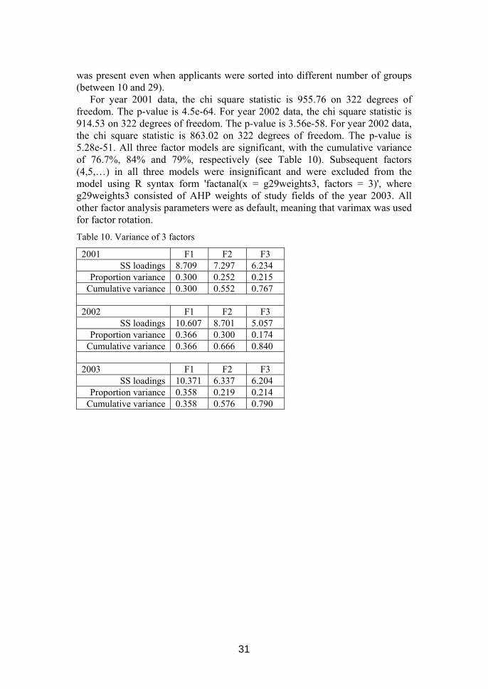
was present even when applicants were sorted into different number of groups (between 10 and 29).

For year 2001 data, the chi square statistic is 955.76 on 322 degrees of freedom. The p-value is 4.5e-64. For year 2002 data, the chi square statistic is 914.53 on 322 degrees of freedom. The p-value is 3.56e-58. For year 2002 data, the chi square statistic is 863.02 on 322 degrees of freedom. The p-value is 5.28e-51. All three factor models are significant, with the cumulative variance of 76.7%, 84% and 79%, respectively (see Table 10). Subsequent factors (4,5,…) in all three models were insignificant and were excluded from the model using R syntax form 'factanal(x = g29weights3, factors = 3)', where g29weights3 consisted of AHP weights of study fields of the year 2003. All other factor analysis parameters were as default, meaning that varimax was used for factor rotation. Table 10. Variance of 3 factors

2001 F1 F2 F3 SS loadings 8.709 7.297 6.234

Proportion variance 0.300 0.252 0.215 Cumulative variance 0.300 0.552 0.767

2002 F1 F2 F3

SS loadings 10.607 8.701 5.057 Proportion variance 0.366 0.300 0.174

Cumulative variance 0.366 0.666 0.840 2003 F1 F2 F3

SS loadings 10.371 6.337 6.204 Proportion variance 0.358 0.219 0.214

Cumulative variance 0.358 0.576 0.790

32

Uniquenesses of variables of 3 factor models of 3 years are given in Table 11. Table 11. Uniquenesses of variables (29 groups of applicants)

Group 2001 2002 2003 Group 2001 2002 2003 V1 0.091 0.075 0.218 V16 0.212 0.129 0.118 V2 0.086 0.038 0.076 V17 0.179 0.103 0.291 V3 0.092 0.051 0.034 V18 0.187 0.132 0.118 V4 0.116 0.100 0.111 V19 0.164 0.189 0.217 V5 0.106 0.090 0.167 V20 0.110 0.174 0.257 V6 0.119 0.118 0.064 V21 0.216 0.167 0.326 V7 0.140 0.086 0.132 V22 0.355 0.132 0.205 V8 0.255 0.145 0.048 V23 0.279 0.204 0.217 V9 0.176 0.046 0.078 V24 0.301 0.189 0.212

V10 0.235 0.053 0.172 V25 0.337 0.198 0.226 V11 0.180 0.129 0.160 V26 0.340 0.203 0.236 V12 0.202 0.107 0.127 V27 0.400 0.175 0.640 V13 0.222 0.124 0.322 V28 0.502 0.438 0.286 V14 0.230 0.200 0.168 V29 0.662 0.520 0.592 V15 0.265 0.320 0.271

Figures 5, 6 and 7 visualize factor weights of each factor in all three years.

Figure 5. Factor weights of factor F1 (all three years).

0

0,1

0,2

0,3

0,4

0,5

0,6

0,7

0,8

0,9

1

V1 V2 V3 V4 V5 V6 V7 V8 V9 V10 V11 V12 V13 V14 V15 V16 V17 V18 V19 V20 V21 V22 V23 V24 V25 V26 V27 V28 V29

2003_12002_12001_1Average

33



0

0,1

0,2

0,3

0,4

0,5

0,6

0,7

0,8

0,9

1

V1 V2 V3 V4 V5 V6 V7 V8 V9 V10 V11 V12 V13 V14 V15 V16 V17 V18 V19 V20 V21 V22 V23 V24 V25 V26 V27 V28

2003_32002_32001_3Average

0

0,1

0,2

0,3

0,4

0,5

0,6

0,7

0,8

0,9

1

V1 V2 V3 V4 V5 V6 V7 V8 V9 V10 V11 V12 V13 V14 V15 V16 V17 V18 V19 V20 V21 V22 V23 V24 V25 V26 V27 V28 V29

2003_22002_22001_2Average

34

The effect of the compression of 29 applicant groups of the year 2001 into 3 factors can be seen in Figure 8.

Figure 8. Weights of study fields based on 3 factors (2001).

The factors represent a reverse scale to 29 applicant groups - factor 1 (F1) represents average and below average applicants, factor 3 (F3) represents the best applicants.

As can be seen, 4-5 most popular study fields are clearly distinctive from the others and their weights increase from factor F1 to factor F3, meaning that they are more popular among the best applicants.

The lower group of study fields (below 0,0035) are also separate from the middle group and their weights decrease from factors 1 to 3, meaning that these study fields are relatively less popular among the best applicants.

The middle group of study fields is divided into two subgroups by factor 2 (at 0,017). Both the tendencies to increase and decrease from factors 1 to 3 are present among weights of the middle group. Examination of the lower group revealed that it only contained self-financed studies (REV) and just 4 self-financed studies belonged to the middle group. As a remark, one speciality may be divided into several study fields based on 2-3 different financing schemes and 2 different languages. The author decided to not build this classification into the preference models directly, because he did not want to make premature assumptions about preferences of applicants - some of them might want to study in either languages, some others might have a self-financed study place as their first preference and state-financed study place as their second preference. And even if the current admission rules do not allow some of these combinations, the rules may change in the future.

0

0,01

0,02

0,03

0,04

0,05

0,06

0,07

0,08

1 2 3

35


The figure of the year 2002 study fields (Figure 9) is basically similar to the previous year - about 9 study fields constitute the first (popular) group, some of the weights increase while others decrease from factors 1 to 3.

The lower group is barely separable from the middle group, but viewed on the logarithmic scale the separation is clear.

The lower group can not be explained by the financing scheme any more, all three financing schemes are present in all three groups.

The nice separation in the year 2001 data might be explained by the rather scarce competition in that year, meaning that almost everybody were bold enough to waste their precious limited preferences on state-financed study fields. This explanation needs further research in the future.

0

0,01

0,02

0,03

0,04

0,05

0,06

0,07

0,08

0,09

1 2 3

36


In the Figure 10 of the year 2003 study fields (9 of them) constituting the popular group are nicely separated. The lower and middle groups are separated only by factors 2 and 3 and that is not visible from this figure, only in log-scale. The lower group mainly consisted of self-financed studies while the popular group consisted of state-financed studies. The results of factor analysis on 3 years show that the applicants fall into three distinct groups and the study fields fall into 3-4 groups. Study field grouping can be further confirmed with cluster analysis, but this was left for future research.

The constructed preference model is so far specific to the admission system of one university. Weights of study fields in different groups can be used to generate stochastic preferences of applicants for each year.

For some stable matching markets, a way to create random tied preferences has to be devised. Also when different study fields have different preference lists over candidates, the division of candidates into groups is not so straightforward any more. In this case either all the applicants have to be treated as a single group when calculating the weights of study fields, or a more elaborate method has to be devised.

The preference model can also be used on some subset of candidates - for example on candidates that have included one specific study field as their first preference (or among the allowed three preferences). If such weights are computed for every study field, then one can use cluster analysis on data that is on continuous ratio scale.

0

0,01

0,02

0,03

0,04

0,05

0,06

0,07

1 2 3

37

2.12 Analysis Results on Stochastically Generated Data The constructed preference model was tested on the preferences of the year

2001. For that, 36 random preference tables (instances) of candidates were generated based on the preference model of that year. Analysis was performed on how the limits on preferences affect the Gale-Shapley matching result. Four different variants of preferences were tried – with 1, 2 or 3 allowed preferences and with unlimited preferences. The matching of unlimited preferences is denoted as match_m. The matchings of limited preferences are denoted as match_me1, match_me2, match_me3.

Only the most interesting results are given here, the location of the rest of the analysis results is explained in the Appendix.

Table 12 shows what will happen when unlimited preferences will be limited to 3 preferences. Table 12. From unlimited preferences to up to 3 preferences in groups 0-14 (2001)

Groups 0-14 (match_m , match_me3) Instance 0 1 2 3 4 5 6 7 8 9 10 11

Lost 119 123 103 110 108 99 105 109 103 104 109 92 Gained 30 35 18 23 28 15 20 24 23 18 23 24

Lost - Gained 89 88 85 87 80 84 85 85 80 86 86 68

Instance 12 13 14 15 16 17 18 19 20 21 22 23 Lost 117 114 120 134 97 101 116 108 102 116 128 111

Gained 35 27 24 23 14 27 28 30 22 24 30 32 Lost - Gained 82 87 96 111 83 74 88 78 80 92 98 79

Instance 24 25 26 27 28 29 30 31 32 33 34 35

Lost 97 92 113 108 98 111 112 121 93 112 111 120 Gained 19 27 30 28 15 27 15 25 18 22 26 18

Lost - Gained 78 65 83 80 83 84 97 96 75 90 85 102 As can be seen from the Lost-Gained rows, this restriction will result in the

net loss of 68-111 study places, the mean is 85.25 and that means about 5.7% of above average applicants (in groups 0-14) lost a study place because of limited 3 preferences. Those applicants would have to find a good strategy to misrepresent their references in order to avoid remaining without a study place. There might not be a single strategy for all and there might not be enough information for applicants to choose the right strategy. The analysis of strategy choice is left for future studies.

The results are similar when comparing matchings based on 3 and 2 allowed preferences (matchings match_me3 and match_me2) in Table 13.

38

Table 13. From up to 3 preferences to up to 2 preferences in groups 0-14 (2001)

Groups 0-14 (match_me3 , match_me2) Instance 0 1 2 3 4 5 6 7 8 9 10 11

Lost 109 104 94 101 88 91 92 98 99 93 94 98 Gained 41 32 43 43 43 39 30 34 31 39 33 31

Lost - Gained 68 72 51 58 45 52 62 64 68 54 61 67

Instance 12 13 14 15 16 17 18 19 20 21 22 23 Lost 95 96 92 85 91 94 88 98 91 91 80 92


Instance 24 25 26 27 28 29 30 31 32 33 34 35

Lost 102 107 101 88 92 94 103 100 95 109 82 101 Gained 31 42 45 36 35 36 39 34 45 42 38 34

Lost - Gained 71 65 56 52 57 58 64 66 50 67 44 67 Between 44-72 candidates will lose their place, the average being 58.5 or

about 4% of above average candidates. Table 14 compares the results of 2 allowed preferences versus only 1 allowed preference. Table 14. From up to 2 preferences to only 1 allowed preference in groups 0-14 (2001)

Groups 0-14 (match_me2 , match_me1) Instance 0 1 2 3 4 5 6 7 8 9 10 11

Lost 204 203 193 204 237 201 200 186 188 211 202 198 Gained 104 67 69 79 89 69 83 68 70 89 94 78

Lost - Gained 100 136 124 125 148 132 117 118 118 122 108 120

Instance 12 13 14 15 16 17 18 19 20 21 22 23 Lost 211 191 208 204 196 227 215 192 215 212 204 213


Instance 24 25 26 27 28 29 30 31 32 33 34 35

Lost 196 189 202 202 181 206 197 200 195 224 225 200 Gained 83 81 80 91 90 86 90 92 85 83 88 93

Lost - Gained 113 108 122 111 91 120 107 108 110 141 137 107 Between 91-152 candidates will lose their place, the average is 120.7 or

about 8.4% of above average candidates. For example in the 1st instance 1219 candidates from groups 0-14 had a place when they were allowed to submit

39

their full preference list. When the allowed preferences was cut to 3, only 1130 candidates from groups 0-14 had a place. When only 2 preferences were allowed, only 1062 candidates from groups 0-14 had a place. When only one preference was allowed, 962 candidates from groups 0-14 had a place. This shows, that 257 candidates from groups 0-14 lost their study place when only the 1st preference was used.

When a large portion of the above average candidates have lost their study place, it would be interesting to know what are the results over all 29 groups, indicating whether candidates from groups 15-28 would benefit from the misfortune of the above average candidates. Table 15 shows what will happen when unlimited preferences will be limited to 3 preferences. Table 15. From unlimited preferences to up to 3 preferences in groups 0-29 (2001)

All groups (match_m , match_me3) Instance 0 1 2 3 4 5 6 7 8 9 10 11

Lost 198 201 183 206 190 185 171 193 187 183 188 169 Gained 195 181 168 187 164 164 162 176 173 183 176 161

Lost - Gained 3 20 15 19 26 21 9 17 14 0 12 8

Instance 12 13 14 15 16 17 18 19 20 21 22 23 Lost 189 175 200 199 163 191 194 168 174 193 200 186


Instance 24 25 26 27 28 29 30 31 32 33 34 35

Lost 168 181 200 179 183 189 167 200 177 175 190 196 Gained 145 168 192 173 168 178 167 195 158 168 180 189

Lost - Gained 23 13 8 6 15 11 0 5 19 7 10 7 There are still many candidates that lose their place, but that is offset by

almost the same number of candidates who were previously without a place who will get a study place. The net loss is between 0-26 candidates, the average being 11.5 or 0.8% from below average candidates.

The results are similar when comparing matchings based on 3 and 2 allowed preferences (matchings match_me3 and match_me2) in Table 16.

40

Table 16. From up to 3 preferences to up to 2 preferences in groups 0-29 (2001)

All groups (match_me3 , match_me2) Instance 0 1 2 3 4 5 6 7 8 9 10 11

Lost 171 179 159 143 147 149 139 168 142 153 158 166 Gained 138 133 130 118 120 118 113 130 110 132 128 126

Lost - Gained 33 46 29 25 27 31 26 38 32 21 30 40

Instance 12 13 14 15 16 17 18 19 20 21 22 23 Lost 152 156 162 152 163 153 139 155 144 143 150 152


Instance 24 25 26 27 28 29 30 31 32 33 34 35

Lost 167 168 160 146 155 170 175 159 154 166 138 160 Gained 140 124 126 131 114 125 143 123 117 150 117 120

Lost - Gained 27 44 34 15 41 45 32 36 37 16 21 40 Between 15-46 candidates will lose their place, the average is 30.75 or about

2% of below average candidates. Table 17 compares the results of 2 allowed preferences versus only 1 allowed preference. Table 17. From up to 2 preferences to only 1 allowed preference in groups 0-29 (2001)

All groups (match_me2 , match_me1) Instance 0 1 2 3 4 5 6 7 8 9 10 11

Lost 322 309 299 317 344 308 319 295 284 336 318 313 Gained 247 240 221 239 262 221 228 209 211 249 236 237

Lost - Gained 75 69 78 78 82 87 91 86 73 87 82 76

Instance 12 13 14 15 16 17 18 19 20 21 22 23 Lost 309 322 312 313 302 301 327 296 326 362 315 307


Instance 24 25 26 27 28 29 30 31 32 33 34 35

Lost 310 291 319 314 297 310 325 316 293 348 329 317 Gained 218 228 236 231 236 229 249 232 225 260 246 230

Lost - Gained 92 63 83 83 61 81 76 84 68 88 83 87 Between 60-119 candidates will lose their place, the average is 81.3 or about

5.9% of below average candidates.

41

As can be seen, limits on preferences will result in huge differences between matchings. The places lost or gained do not represent all changes between these matchings - many of the candidates will simply get a worse study place and some will get a better place. For example, in the 1st instance, the difference between matchings match_m and match_me3 is 454 different study places for candidates. The difference between match_me3 and match_me2 is 351 and the difference between match_me2 and match_me1 is 636. The difference between match_m and match_me1 is smaller than 454+351+636=1441, because a candidate can lose his place when the preference limit is set to 3 allowed preferences and limiting the preferences further may give that candidate a new place (or get back the old one).

The analysis based on stochastic preferences is still in a preliminary phase, but the preliminal results show that the negative effect of limiting the number of allowed preferences is considerable and these effects should be analysed in more detail. All applicants would have to find a good strategy to submit preferences that would give them best chances to get a study place. There might not be a single strategy for all and there might not be enough information for applicants to choose the right strategy.

The differences between different matchings can also be compared based on the total regret of each of these matchings, where the regret of each participant is the position of the given partner in his preferences. The total regret is the sum of regrets over all participants.

If the participants of the central matching system SAIS agree to allow the state to enforce unstable matchings, then a whole new range of possible matching methods will be available. TSP (Traveling Salesman Problem) algorithms, for example the Hungarian method, can be used to minimize the total regret. With fully random preferences on both sides the minimum total regret is on average about 20% smaller than the minimum total regret on stable matchings (master thesis of Veskioja, 2000). With the proposed preference model it is possible to estimate this difference on more realistic circumstances. Roth has showed in his computational experiments with simple markets with random k-length preferences, that the size of the set of stable matchings is a function of the market size and length of preference lists (1999c).

2.13 Breaking of Tied Preferences The proposed preference model has one significant shortcoming - it doesn't

generate tied preferences. In the future this preference model has to be extended to do that. Ties can possibly occur on both sides of the market - candidates and study places.

For breaking of ties, the literature (Roth and Sotomayor 1990) mostly suggests that it can be arbitrary, because if a candidate is indifferent between several alternatives, he does not mind when the central matching system changes his tied preferences into arbitrary strict rankings. The necessity of breaking the ties comes from the fact, that in the stable marriage markets with ties and incomplete lists of preferences (in 1:1 and 1:N markets) there always

42

exists a weakly stable matching (Iwama et al., 1999), but the sizes of stable matchings may vary and finding maximum cardinality matching in 1:1 market is NP-complete (Iwama et al., 1999) and even the approximation is APX-hard (Halldórsson et al., 2002). Gent et al. (2001, 2002a, 2002b) have published some interesting experimental results on that type of markets.

A simple way to break the ties would be to use the AHP weights of the preference model - ties will be broken based on the preferences of all participants. A more complex and perhaps more precise would be to find candidates with similar preference lists and break the ties based on only similar candidates' preferences.

The usefulness of a tie-breaking procedure has to be viewed in the context of a matching method - if a maximum cardinality minimum total regret stable matching is sought, then the tie-breaking method has to be chosen based on these criteria.

43

4. Majority Voting in Stable Marriage Problem with Couples

Many markets also require taking into account some additional constraints - for example in HR a pair of residents may have formed a couple and prefer to find a placement at the same hospital, or at least work in the same city. In this case, the couple submits rank ordered preferences over acceptable pairs of hospitals. After acceptable pairs of hospitals the couple can give rank ordered preferences over single pairs of hospital – couple member, where one of the members of the couple is left without a pair. In this thesis these mentioned constraints will be called couple constraints.

Matching markets with couple constraints may not have any stable matchings (Roth and Sotomayor, 1990). In that case it is natural to use majority voting to find the best matching. Veskioja and Võhandu (2004a) have proposed a matching framework that always gives a matching, although it is obviously not always an optimal matching. The framework is based on a genetic algorithm that uses intermediate or approximate matchings from other matching algorithms. The best voted matchings from each population are chosen by the tournament ranking. For ranking a simple heuristical greedy tournament method based on monotone systems is proposed and a value function for it.

In paragraph 2.14 are the definitions of domination and the core of a game (Roth and Sotomayor, 1990; pages 54-55, 166-167). The definitions are needed to understand the importance of stability and the core. In paragraph 2.15 an example of a matching model with couple constraints is used from Roth (Roth and Sotomayor, 1990) to show that it has intransitivities and every dominance path of matchings leads to the cycle of unstable matchings. Paragraph 2.16 discusses problems in choosing matchings for the tournament. Paragraph 2.17 gives the description of the proposed matching framework.

Paragraph 5 describes tournament problem as a type of feedback arc/edge set problem on a directed unweighted graph. The proposed tournament method is described together with performance results.

2.14 The Core Of A Marriage Game The following are the definitions of domination and the core of a game (Roth

and Sotomayor, 1990; pages 54-55, 166-167). Feasible outcomes of a game are all possible outcomes given the rules of the

game, the set of players and preferences of players over outcomes. Definition 4.1.1. For any two feasible outcomes x and y, x dominates y if and only if there exists a coalition of players S such that (a) every member of the coalition S prefers x to y; and (b) the rules of the game give the coalition S the power to enforce x (over y). For this reason, if x dominates y, one might expect that y will not be the outcome of the game. This leads us to consider the set of undominated outcomes.

44

Definition 4.1.2. The core of a game is the set of undominated outcomes. The domination conditions of definition 4.1.1 can be relaxed, assuming that the coalition can make side-payments to those players that are indifferent between outcomes x and y. Definition 4.1.3. For any two feasible outcomes x and y, x weakly dominates y if and only if there exists a coalition of players S such that (a) every member of the coalition S prefers x at least as much as y; and (b) at least one member of the coalition S prefers x to y; and (c) the rules of the game give the coalition S the power to enforce x (over y). Definition 4.1.4. The core of a game defined by weak domination is the set of weakly undominated outcomes. According to the first two definitions the core of the one-to-one matching market equals the set of stable matchings (Roth and Sotomayor, 1990, paragraph 3.1, theorem 3.3). When preferences are strict, the two cores coincide in the one-to-one matching model, but not in the many-to-one model. However, when hospital preferences are responsive (as defined in Roth and Sotomayor, 1990, definition 5.2, page 128), and when preferences over individuals are strict, the set of stable matchings coincides with the core defined by weak domination (Roth and Sotomayor, 1990; proposition 5.36, page 167). In the many-to-one (or one-to-one) matching model with couples, the set of stable matchings and consequently the core may be empty (Roth and Sotomayor, 1990, theorem 5.11, page 141). Lets look at the example that Roth & Sotomayor gave to illustrate this problem.

2.15 An Empty Core Example Of Many-To-One Model With Couples The following example is taken from Roth & Sotomayor (Roth and

Sotomayor, 1990; theorem 5.11, page 141). Consider the market with hospitals H = {H1, H2, H3, H4} each of which

offers exactly one position and each of which has strict preferences over students S = {s1, s2, s3, s4} as given in Table 18. The students consist of two married couples, {s1, s2} and {s3, s4}. Each couple has strict preferences over ordered pairs of hospitals, as given in Table 18.

45

Table 18. Preferences of 4 hospitals and 2 couples

Hospitals' rank orders Couples' rank orders H1 H2 H3 H4 {s1,s2} {s3,s4} s4 s4 s2 s2 H1H2 H4H2 s2 s3 s3 s4 H4H1 H4H3 s1 s2 s1 s1 H4H3 H4H1 s3 s1 s4 s3 H4H2 H3H1 H1H4 H3H2 H1H3 H3H4 H3H4 H2H4 H3H1 H2H1 H3H2 H2H3 H2H3 H1H2 H2H4 H1H4 H2H1 H1H3

Thus couple {s1, s2} has as its first choice that s1 be matched with H1 and s2 with H2, and has its last choice that s1 be matched with H2 and s2 with H1. The 24 individually rational matchings of students to hospitals are listed in Table 19, along with the reason that each such matching is unstable. Table 19. Matchings of 4 hospitals and 2 couples

Matching H1 H2 H3 H4 Unstable with respect to

1 s1 s2 s3 s4 s4 , H2 2 s1 s2 s4 s3 s4 , H2 3 s1 s3 s2 s4 s2 , H4 4 s1 s3 s4 s2 s4 , H1 5 s1 s4 s2 s3 s2 , H4 6 s1 s4 s3 s2 s4 , H1 7 s2 s1 s3 s4 s4 , H1 8 s2 s1 s4 s3 s4 , H2 9 s2 s3 s1 s4 s2 , H4

10 s2 s3 s4 s1 s4 , H1 11 s2 s4 s1 s3 s2 , H4 12 s2 s4 s3 s1 s4 , H1 13 s3 s1 s2 s4 s4 , H2 14 s3 s1 s4 s2 s2 , H3 15 s3 s2 s1 s4 s2 , H4 16 s3 s2 s4 s1 s2 , H3 17 s3 s4 s1 s2 s1 , H1 18 s3 s4 s2 s1 s2 , H1 19 s4 s1 s2 s3 s4 , H2 20 s4 s1 s3 s2 s2 , H3 21 s4 s2 s1 s3 s2 , H4 22 s4 s2 s3 s1 s2 , H3 23 s4 s3 s1 s2 s3 , H3 24 s4 s3 s2 s1 s4 , H4

46

Thus matching 1, which assigns student si to hospital Hi, i=1,…,4, is unstable because both hospital H2 and couple {s3, s4} would prefer that student s4 be matched with H2. (This follows since H2 prefers s4 to s2, and {s3, s4} prefers H3H2 to H3H4.) The domination graph between matchings is shown on Figure 11.

Figure 11. Domination graph

If we study the dominance between these matchings, it becomes clear that every dominance path leads to the following cycle of unstable matchings {6, 20, 19, 5} (in the order of dominance), entering the cycle from one of the matchings 6, 20 or 5.

Roth and Sotomayor (Roth and Sotomayor, 1990, page 142) formulated an open question whether there exist plausible restrictions on the preferences of the couples that would insure that stable matchings always exist. The author of this thesis suggest that studying these restrictions in the context of minimizing transitivity faults is a more fruitful approach. If there are few enough transitivity faults left in the tournament ranking, then at some point stable matchings should emerge.

As soon as the players of the marriage game realize that there is no stable outcome, they start looking for a way out of this vicious cycle, at least in a cooperative game. In doing that the players will start seeking coalitions to reach an outcome through majority voting. The existence of cyclic domination also means the existence of intransitivity. So to reach an outcome, the players have to vote between pairwise matchings as in a tournament.

Note that the only way to avoid a tournament is to not let the existence of the cycle to become common knowledge. The blocking pair (or one of them) to the last matching in the cycle can choose to not form a pair by themselves, but to seek coalition partners to seek out the best matching in the cycle for the coalition and to dominate over other matchings.

47

2.16 How To Select Matchings For The Tournament When using majority voting in a full tournament one has to have a relatively

small set of matchings (up to thousands or tens of thousands). Since the number of individually rational matchings is combinatorial, the selection of matchings for majority voting tournament becomes critical.

One solution is to hold a tournament between the set of matchings in the cycle of unstable matchings. A stable matching searching algorithm can be used to find the cycle.

It would be interesting to know whether the outcome of the majority voting tournament result depends on the subset of individually rational matchings, which always includes the cycle of unstable matchings. When looking at the following dominance path {18; 12; 22; 24; 3; 4; 23; 20; 19; 5; 6}, the minimum number of transitivity faults is 2 and there are several rankings with that number of faults. One ranking with 2 faults is (12; 24; 22; 6; 5; 3; 18; 23; 19; 20; 4). As can be verified, if the matching 12 is included (and all subsequent matchings along the dominance path to the cycle) in the tournament, it always wins.

In the complete information game the matchings need not even be restricted to the cycle and the path leading to the cycle, but all the matchings in the majority voting are “fair game”. If all matchings were to be included in the tournament, then one ranking order in our example would be (12; 24; 5; 22; 20; 6; 1; 3; 18; 23; 11; 9; 10; 4; 17; 21; 2; 19; 7; 15; 13; 16; 8; 14). The number of transitivity faults is 7. It is not known to the author of this thesis whether this ranking is optimal or not.

If the stable marriage model includes couples, then the complexity of finding if there exists a stable matching is NP-complete and “logspace P-hard” (Ronn 1986, 1987). So for large markets with couples it may not always be practical to find a stable matching even when one exists. In this case a probabilistic matching algorithm can be used to find a stable matching or a cycle of unstable matchings. One promising approach would also be using a genetic algorithm together with majority voting tournaments to search for the best matching.

2.17 Matching Framework The proposed framework is based on a genetic algorithm. A genetic

algorithm is very easy to implement. It consists of the following basic steps - proper coding of the problem instance, generating initial population of solutions (matchings), using a fitness function to evaluate each solution, finding the best solutions and letting them live, creating offsprings by using crossovers, initiating random mutations in the (genetic) code of the solution.

Besides being able to search the solution space by itself, the genetic algorithm can also accept solutions from other algorithms that solve the same or a similar problem. Not many of matching algorithms can do that. Many approximation and heuristic matching algorithms are candidates to supply the genetic algorithm with good approximate solutions. For example, almost any matching market can be reduced to 1:1 matching market with complete preferences and without ties, thus enabling to use the Gale-Shapley algorithm to

48

find one-side optimal solutions to the reduced problem. These solutions are not guaranteed to be optimal to the original problem, but these are good enough for the framework that uses a genetic algorithm. By using solutions from different matching algorithms, that have different complexity phase transitions, a genetic algorithm can minimize the cost of complexity phase transitions. This framework can also make use of parallel computation.

The coding of a stable matching solution should be as simple as possible - a list of men (or a list of women) and their partners. The pairs are ordered by the original order of men in the input data, but the sequential number of men are not shown. If a man has a partner, then the sequential number (or id) of his partner is shown. If a man is single, then we can mark his own sequential number as his partner.

Another way of coding is to also code in the constraints of the problem, but the constraints can be built into and evaluated by the fitness function. With constraints in the genetic code, the crossover function would be much more difficult to implement. That is why the author of this thesis opted for the simple coding.

Cyclic crossover is used in genetic algorithms for Traveling Salesman Problems (TSP), see for example Oliver, Smith and Holland (1986). Brian Aldershof and Olivia M. Carducci (1999) have described the use of cyclic crossover in marriage models.

A fitness function is used to select the best solutions. It is wise to construct a relative fitness function that compares two solutions, instead of an absolute fitness function. Majority voting between matchings suits well as a relative fitness function.

There are several ways how to find the best solutions from the population. A simple approach to tournament ranking is called tournament selection. In tournament selection, some number of individuals are randomly chosen from the population, the best from the chosen individuals are copied to the intermediate population (Blickle et al., 1995). This is repeated until the selection number is reached. Often tournaments are only held between two individuals (called binary tournaments).

A major problem with comparing solutions is the transitivity of ranking. Transitivity requires that if solution a is better than solution b and solution b is better than solution c, then solution a must be better than solution c. With special constraints (for example permitting couples to submit combined preferences) this transitivity may not always hold. Tournament selection does not minimize transitivity inconsistencies. In this situation it is necessary to use a full or a partial tournament to get a correct ranking.

49

5. Tournaments as Feedback Set Problems Let G = (V;E) be a graph with vertex set V and arc set E. A path in G

connecting vertex u to vertex v is a sequence of arcs e1, …, er in E, such that e1=(vi, vi+1), i=1, …, r with v1=u and vr+1=v. A cycle C in G is a path C=(v1, …, vr), with v1=vr. A feedback arc set of G is a subset of arcs S ⊆ E such that each cycle in G contains at least one arc in S. Let w be a function that assigns a nonnegative weight to each arc of G. Then the weight of a feedback arc set is the sum of the weights of its arcs, and a minimum feedback arc set of a weighted graph (G,w) is a feedback arc set of G of minimum weight (Festa, Pardalos & Resende, 2001), the problem of finding a minimum feedback arc/edge set is often denoted as a FAS problem. The complexity of the FAS problem is NP-complete and APX-hard.

If the arcs E in graph G are directed and unweighted (all equal to 1), then that graph represents a tournament, where vertexes represent players and arcs represent the result of a pairwise comparison. The possible results of a pairwise comparison in this type of graph are 0:0, 0:1, 1:0, 1:1.

For a given tournament there can be many optimal rankings with the same size of the minimum feedback arc set. If many (ar all) equally good rankings have been found, then one can use additional criteria to choose the best ranking. One possible solution is to construct a new voting table from these rankings, transform it into a new tournament table and again find optimal or near-optimal rankings. Another solution is to use Kemeny-Snell median (1960, 1962) or some other distance metrics to choose from the best rankings. Yet another solution is to employ a lottery between the best rankings. Some other alternatives have been discussed by Stob (1985). The study of additional criteria will be left for future studies.

Optimal FAS methods are appropriate to use for ranking up to 10 or 20 objects. The problem is, that the time spent by the optimal method to solve a specific instance is not known beforehand. For practical applications it is preferable to use an approximate or heuristic method to find a good solution and after that use the available time to verify it with an optimal method. The choice of a method depends on the size of the problem and on the available time. One very successful approach is to use a metaheuristic, such as GRASP (Festa, Pardalos and Resende, 2001), to combine several different heuristic methods. GRASP is a greedy random adaptive search method, that is being used to solve many different combinatorial NP-complete problems, for a comprehensive and up-to-date list see Festa and Resende (2004). The essence of GRASP is that in each iteration a semi-random (tournament ranking) sequence is generated based on a greedy evaluation function (or several functions). The initial solution is then locally optimized using various techniques. See Resende and Ribeiro (2003) for a more detailed description of GRASP. Festa, Pardalos and Resende (2001) have described a variant of GRASP to solve the minimum feedback vertex set problem and they have made available a set of random graphs with

50

different size and density (http://www.research.att.com/~mgcr/data/) for benchmark purposes.

My supervisor has successfully been using a monotone-systems (Mullat, 1976) based greedy heuristic method before (Võhandu, 1989, 1990) and he suggested to use that or to find a new value function. As a result of that study a new variant of a monotone-systems based greedy heuristic was created. Paragraph 2.18 describes a general structure of monotone-systems based methods. Paragraph 2.19 describes the proposed tournament method. Paragraph 2.20 describes the construction of a testing experiment. Paragraph 6.4 describes 2.21 testing results of the tournament method. In Paragraph 6.5 a possibly new global optimization technique is given that can be used together with the monotone-systems based method or with GRASP. The two proposed methods have been tested on large tournament tables and these results are given in paragraph 2.23. For more information about monotone systems, see http://www.datalaundering.com/.

2.18 An Algorithm Based On A Monotone System Definition 5. (A weakly) monotone system is a system built on a set of objects, such that objects are weighted by a value function and after removal of one object from the set all the weights of other objects still in the set change monotonically in one direction (increase or decrease) or stay on the same level. Algorithms based on such a simple monotone system work as follows: Step 1. Evaluate all objects in the set. Step 2. Find the weakest object (with the smallest (largest) weight), and remove it from the set. If there are several weakest objects, then recursively apply the tournament algorithm to the set of weakest objects. If at any stage of the recursion any object was removed from the set of weakest objects, then backtrack. If the set of weakest objects still contains more than one object, then compare the weights from the previous iteration and choose an object that is more similar to the previously removed object. If the weights in all the previous iterations are the same, then according to the value function these objects are equivalent and we can remove any one of those (usually the first object will be removed). Step 3. If there are still objects in the set, then continue from Step 1. Any given algorithm always removes the object with the smallest weight, or the largest weight. Algorithm cannot change the choice function (min, max) during the course of action. Value function can be chosen relatively freely, as long as it satisfies monotonicity condition. The sequence of removal of objects constitutes object ranking.

2.19 Tournament Method Based On A Monotone System To construct a tournament method a value function has to be defined and an

ordered set of object removal criteria has to be selected. The proposed method

51

makes use of both the number of wins (rowsums) and losses (column sums) in the tournament table T. The method iteratively finds the weakest object, removes it from the tournament table and adds it to the ranking. The last remaining object in the tournament table is the winner. The process of finding the weakest object to remove is also iterative – the weakest objects are selected by the minimum number of wins and then by the maximum number of losses in the remaining subset of the weakest objects. This iterative minimax selection is used until either only one weakest object remains or the last minimax selection was not able to reduce the number of weakest objects. In the latter case the first remaining weakest object in the original ranking is removed. The algorithm H is as follows:

1. Find rowsums, column sums. 2. Set of weakest objects = set of objects remaining in the tournament table 3. Select from the set of weakest objects the objects with the smallest

rowsums (the least number of wins). 4. If there was a selection, then mark the occurrence of it. Recompute

selection table rowsums and column sums. If a single weakest object is remaining, then resume from step 8.

5. Select from the set of weakest objects the objects with the largest column sums (the biggest number of losses).

6. If there was a selection, then mark the occurrence of it. Recompute selection table rowsums and column sums.

7. If the set of weakest objects contains more than one object and the selection has occurred during steps 3 and/or 5, then resume from step 3.

8. Add the first remaining weakest object to the top of the ranking list and remove it from the tournament table, recompute tournament table rowsums and column sums.

9. If the tournament table still contains some objects, then resume from step 2.

10. The end.

The finding and removal of the weakest object has a maximum complexity of O(N2), because each remaining object in the set of weakest objects can be removed only once. The removal of an object from either tournament table or from the set of weakest objects has a time complexity of O(N), because the row of the removed object has to be negated from rowsums and the corresponding column has to be negated from column sums. So, the algorithm has a polynomial maximum time complexity O(N3).

In a majority voting, all the players have to vote (pairwise) between the matchings. Voting results constitute the voting table v. Voting table for the cycle of unstable matchings {6, 20, 19, 5} used in Paragraph 2.16 is given in Table 20.

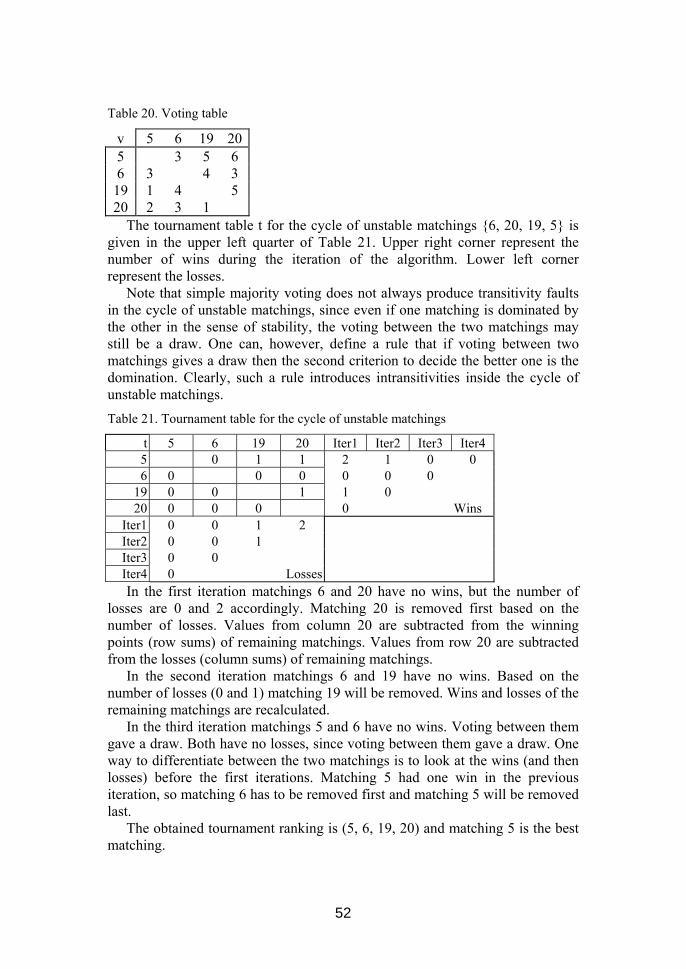
52

Table 20. Voting table

v 5 6 19 205 3 5 6 6 3 4 3

19 1 4 5 20 2 3 1

The tournament table t for the cycle of unstable matchings {6, 20, 19, 5} is given in the upper left quarter of Table 21. Upper right corner represent the number of wins during the iteration of the algorithm. Lower left corner represent the losses.

Note that simple majority voting does not always produce transitivity faults in the cycle of unstable matchings, since even if one matching is dominated by the other in the sense of stability, the voting between the two matchings may still be a draw. One can, however, define a rule that if voting between two matchings gives a draw then the second criterion to decide the better one is the domination. Clearly, such a rule introduces intransitivities inside the cycle of unstable matchings. Table 21. Tournament table for the cycle of unstable matchings

t 5 6 19 20 Iter1 Iter2 Iter3 Iter4 5 0 1 1 2 1 0 0 6 0 0 0 0 0 0

19 0 0 1 1 0 20 0 0 0 0 Wins

Iter1 0 0 1 2 Iter2 0 0 1 Iter3 0 0 Iter4 0 Losses

In the first iteration matchings 6 and 20 have no wins, but the number of losses are 0 and 2 accordingly. Matching 20 is removed first based on the number of losses. Values from column 20 are subtracted from the winning points (row sums) of remaining matchings. Values from row 20 are subtracted from the losses (column sums) of remaining matchings.

In the second iteration matchings 6 and 19 have no wins. Based on the number of losses (0 and 1) matching 19 will be removed. Wins and losses of the remaining matchings are recalculated.

In the third iteration matchings 5 and 6 have no wins. Voting between them gave a draw. Both have no losses, since voting between them gave a draw. One way to differentiate between the two matchings is to look at the wins (and then losses) before the first iterations. Matching 5 had one win in the previous iteration, so matching 6 has to be removed first and matching 5 will be removed last.

The obtained tournament ranking is (5, 6, 19, 20) and matching 5 is the best matching.

53

2.20 The Construction Of An Experiment Evaluating heuristic methods is very problematic. A method can give an

optimal result on some instances, yet on other instances it can give a result that is far from optimal. That is why proper construction of an evaluation experiment has to be considered extremely important.

It was decided to test the proposed heuristic method against all possible general tournament tables (with ties allowed) of sizes 5x5 and 6x6 and all 1:0 tournament tables of size 7x7. The results from the proposed method were compared to the actual number of minimum transitivity faults found by the brute force approach that tries out all possible rankings.

As the author of this thesis has special interest in tournaments that are based on decision-makers preference lists, he also considered trying all possible preference lists (with ties allowed). This however would have restricted him only to the tournaments of size 4x4, since there are 1215450 different combinations of preference lists. For preference lists of size 5, the number of combinations would be a very large number indeed. That is why the decision was made to exclude the influence of preference lists to tournaments from the analysis. It is quite conceivable, that not all tournament tables can be achieved from preference lists. If that is the case, then the comparison of different heuristic tournament methods has to be done separately for preference lists and tournament tables, and for tournament tables only. In this thesis only the latter is considered.

For the construction of all tournament tables it is convenient to view two elements tij and tji as having a single state out of three possible states (0;0), (0;1), (1;0). For 1:0 tournament tables there are only two possible states (1;0), (0;1). Now we can mark this combined state only to the elements below the main diagonal (tij, i > j). If we enumerate all elements below the main diagonal so that the number of the element corresponds to the rank in a base3 number (base2 for the 1:0) as in the Table 22, then we can describe every tournament table with a unique number. Table 22. Enumeration of elements below the main diagonal

1 2 3 4 5 6

54

As an example of the coding, the unique index of a 6x6 table with ties in Table 23 is 110768 in base10. Table 23. 6x6 table no. 110768

0 0 0 0 1 0 0 0 0 1 0 1 0 0 0 0 1 1 0 0 1 0 0 1 0 1 0 1 0 0 1 0 0 0 1 0

The number of ranks in a base3 index for a table of size n is m=n(n-1)/2 and

the number of all possible generalized tournament tables of size n is then 3m. There are 729 tables of size 4x4, 59049 tables of size 5x5 and 14348907 tables of size 6x6. For 1:0 tournaments there are 32768 tables of size 6x6 and 2097152 tables of size 7x7. In fact, one does not have to look through all variants, because the ranking should not depend on the original order of elements i.e. on the order of rows and columns. The unique indexes of permutation tables of one variant table were obtained and marked at the same time when the true minimum number of faults was computed by trying all possible sequences. When the program later on reached to the index of a table that was marked, it was omitted, because it was a permutation table for some previously encountered table. Of course one also had to make sure if the tournament method results (the number of faults in a resulting ranking) are dependent on the original ranking of rows or columns. For that, modified recursive algoritm was used at step 8, where it was tried to remove each one of the remaining weakest objects and then recursively call the proposed tournament method to order the remaining objects and to verify whether the recursive calls result in different number of transitivity faults or not.

Using the above-mentioned reductions the number of 5x5 generalized tournament table variants shrunk about a 100-fold, to 582. However, it was still necessary to verify all 59049 of the variants, but it was done just once.

All biggest memory consuming elements of the program were part of the experimentation program, not part of the proposed tournament method. The memory complexity of the tournament method is O(N2).

2.21 Testing results of the tournament method Very little can be said about tournament tables of size 5x5. For this size,

method H always gives a ranking that has a minimum number of transitivity faults, also meaning that in all these cases the method does not depend on the original sequence of objects.

For 1:0 tournaments of size 6x6, only two tables cause method H to give wrong results - tables 20 and 24 (Table 24, Table 25).

55

Table 24. 6x6 1:0 tournament table no. 20

0 1 1 1 1 0 0 0 1 1 1 1 0 0 0 1 1 0 0 0 0 0 1 1 0 0 0 0 0 1 1 0 1 0 0 0

For table no.20 method H gives a ranking 2-6-1-3-4-5 with 3 faults. The best ranking is obviously 1-2-3-4-5-6 with 2 faults. Table 25. 6x6 1:0 tournament table no. 24

0 1 1 1 1 0 0 0 1 1 1 0 0 0 0 1 1 1 0 0 0 0 1 1 0 0 0 0 0 1 1 1 0 0 0 0

For table no.24 method H gives a ranking 6-1-2-3-4-5 with 3 faults. The best ranking is obviously 1-2-3-4-5-6 with 2 faults.

For 2097152 1:0 tournament tables of size 7x7, there are 36 tables where method H is not optimal. The decimal indexes of these tables are: (20, 24, 36, 40, 41, 48, 49, 169, 177, 297, 305, 310, 314, 368, 550, 553, 558, 561, 566, 570, 612, 616, 624, 636, 675, 737, 803, 807, 817, 1073, 1082, 1328, 1329, 1392, 1460, 1584).

For 14348907 tournament tables of size 6x6, there are 81 tables where method H is not optimal. The indexes of these tables are: (82755, 91571, 110768, 286240, 287683, 614196, 622985, 623012, 718780, 720700, 737491, 737734, 738220, 738463, 740374, 740383, 777586, 777829, 778315, 779722, 779749, 797269, 798970, 799423, 799432, 799462, 799468, 799942, 800175, 800177, 800185, 800193, 800195, 800428, 817681, 818627, 818653, 819106, 819124, 819127, 819133, 819145, 819151, 819625, 820085, 820111, 839525, 839527, 839768, 862855, 863105, 863130, 863132, 878648, 878891, 878893, 882781, 2372152, 2391592, 2393293, 2393758, 2393764, 2393773, 2393785, 2393791, 2394265, 2394500, 2394518, 2394751, 2433848, 2433850, 2434091, 2453561, 2457916, 2457917, 2479318, 2984245, 2984251, 2988655, 7174543, 7174561). The table indexed 82755 shows that graph reduction methods as described in Festa, Pardalos and Resende (2001) should be used in each iteration. At the moment the proposed method does not use these reductions.

Ali, Cook and Kress (1986) have conducted a similar study where they compared two heuristic tournament algorithms, namely Iterated Kendall method (IK) that is derived from a Kendall method (1962) and p-connectivity method by Goddard (1983). These two methods were tested on all tournament tables of size 5x5 with no ties. The Iterated Kendall method was reported to give the wrong number of minimum violations on two tables, while the p-connectivity method was reported to give the wrong number of minimum violations on four

56

tables and four other tables would lead to the situation of unbreakable ties (and hence no solution). As the author of this thesis understands these two methods were not tested on 5x5 tournament tables that include ties.

For a comparison, 2 tournament tables from an article from Goddard (1983) were also tried. Table 26. 13x13 table (without ties) from Goddard

0 1 0 1 1 1 0 1 1 1 1 1 10 0 0 1 0 1 1 1 1 1 1 1 11 0 0 1 1 1 0 0 1 0 1 1 10 0 0 0 1 0 0 1 1 1 1 1 10 1 0 0 0 0 1 1 0 1 1 1 00 0 0 1 0 0 1 0 1 1 0 1 11 0 1 1 0 0 0 0 0 0 1 0 10 0 1 0 0 1 1 0 0 0 1 0 10 0 0 0 0 0 0 0 0 1 0 1 10 0 0 0 0 0 0 1 0 0 0 1 10 0 0 0 0 0 0 0 0 1 0 0 10 0 0 0 0 0 1 1 0 0 0 0 10 0 0 0 1 0 0 0 0 0 0 0 0

For the 13x13 table (Table 26) method H gave a ranking (1-5-2-8-7-3-6-4-9-10-12-11-13) with 11 violations as compared to 13 (1-2-3-5-6-7-4-8-9-10-12-11-13), that was reported by Goddard. The best minimum number of violations in this case is 8 (3-1-2-6-4-5-9-10-12-8-7-11-13). That ranking was reported by Ali, Cook and Kress (1986). This was also reached by Võhandu's more complicated variant of a monotone system based tournament method (1989, 1990), which has the same time complexity with the proposed method. Võhandu's method has also given rankings with minimum violations on many of the above-mentioned 6x6 tables, that proved difficult to the proposed method. However, the author of this thesis has not yet extensively tested Võhandu's method against all tournament tables of a given size and that is why it is not possible to report about its efficiency yet.

The 10x10 table from Goddard (1983) in Table 27 was reported to have 5 transitivity faults (1-4-2-3-5-7-6-9-8-10). The proposed method gave a ranking (3-2-1-5-7-4-6-8-10-9) with 4 faults, as did Ali, Cook and Kress with a slightly different ranking.

57

Table 27. 10x10 table (without ties) from Goddard

0 0 1 0 1 1 1 0 0 1 1 0 0 0 1 1 0 0 1 1 0 1 0 0 0 0 1 1 1 1 0 0 1 0 0 1 0 1 0 1 0 0 0 0 0 0 1 1 0 1 0 0 0 0 0 0 0 1 1 1 0 1 0 1 0 0 0 1 1 0 0 0 0 0 0 0 0 0 0 1 0 0 0 0 0 0 0 0 0 0 0 0 0 0 0 0 1 0 0 0

The author of this thesis has also used the test tables of Festa, Pardalos and Resende (2001, http://www.research.att.com/~mgcr/data/), that they have made available.

On these tables an additional optimization technique was used, called a global optimization, as opposed to local optimization. In local optimization, a subsequence of a ranking is analysed separately for a more optimal ranking. In the proposed global optimization, a table of fault changes is computed for one-object movements.

2.22 Global Optimization in a FAS problem Let there be a tournament table T, with a pairwise comparison of objects i

and j denoted as tij. Let C be the table of fault changes cij. Then the fault change for moving an object i back in the tournament sequence to the position j (i<j) is as follows: cji = Σ (tki - tik), (k=i, .., j), (i<j)

The fault change for moving an object i forward in the tournament sequence to the position j (i>j) is as follows: cji = Σ (tki - tik), (k=j, .., i), (i>j)

If there are positive values in the change table C, then moving an object i to a position j will reduce the number of faults (feedback arcs). An example of a tournament table T and a corresponding change table C is given in Table 28. Table 28. Tournament table T and a corresponding change table C

T C0 0 0 0 0 1 2 01 0 0 1 1 0 1 01 1 0 0 2 1 0 10 0 1 0 2 0 1 0

A simple method that was used is to find the biggest positive values of C and choose the move whose original or destination position is closest to the upper left corner of the table C. In this way the front of the sequence is optimized first. In the example depicted in Table 28, there are 3 moves, that would reduce the feedback arc set by 2 arcs – (0,2); (2,0); (3,0). According to the rules the first

58

choice has to be made, because all moves include position 0, and in this situation the first move will be selected (moves are ordered first by row index, then by column index). After a move has been made, the change table has to be recomputed. The moves are made iteratively until there are no more positive values in the change table. The complexity of this method is O(N4). The author of this thesis has not found any reference to a previous description of such a global optimization technique, but due to the extreme simplicity of the method it is unlikely that it is a unique result.

The change table can also be used to exhaustively or selectively search through all possible move combinations (using bounded search), but that experiment is left for future studies. In the following paragaph are the results of using a monotone-systems approach together with global optimization on the test tables of Festa, Pardalos and Resende (2001), that they have made available.

2.23 Results on large tournament tables Festa, Pardalos and Resende (2001) have made available 40 large random tournament tables with 50-1000 vertices and 100-30000 arcs (http://www.research.att.com/~mgcr/data/). Each table includes ties that are coded as 0:0 and ties coded as 1:1. Original tables are denoted as T1. The author of this thesis has tried the proposed methods on the original tables, and on tables where all 1:1 ties are recoded as 0:0. Tables with only 0:0 ties are denoted as T0. A table only consisting of ties of type 1:1 are denoted as T11. The results are given in Table 29. The resulting table after the application of a monotone-systems based heuristic described in paragraph 2.19 is denoted as H(T). The resulting table after the application of global optimization is denoted as G(T). The second column gives the number of faults in T1 caused by 1:1 ties. The third column gives the result of first using the sequence of H(T1) to sort T0 and then applying G( H(T1), T0). For example, filename ‘P50-900.dat’ contains a graph (as a table) with 50 vertices and 900 arcs, of which 162 are ties of type 1:1. H(T1) shows that the heuristical method H gives 348 feedback arcs on the original table, whereas the same method gives 169 feedback arcs on a table where the 1:1 ties have been replaced with 0:0 ties (H(T0))), meaning that pure 0:0 encoding of ties gives 169 + 162 = 331 feedback arcs on the original table – a better result. When a global optimization is used on H(T0), then the result G(H(T0)) is even better: 148 + 162 = 310 faults on the original table.

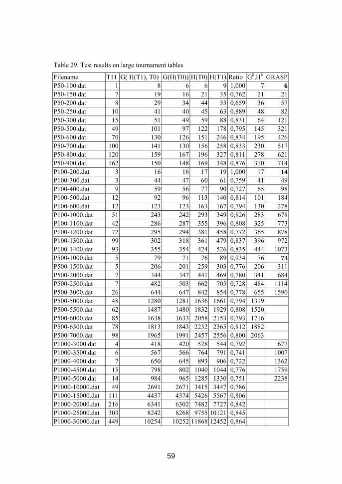
59

Table 29. Test results on large tournament tables

Filename T11 G( H(T1), T0) G(H(T0)) H(T0) H(T1) Ratio G8,H8 GRASP P50-100.dat 1 8 6 6 9 1,000 7 6 P50-150.dat 7 19 16 21 35 0,762 21 21 P50-200.dat 8 29 34 44 53 0,659 36 57 P50-250.dat 10 41 40 45 63 0,889 48 82 P50-300.dat 15 51 49 59 88 0,831 64 121 P50-500.dat 49 101 97 122 178 0,795 145 321 P50-600.dat 70 130 126 151 246 0,834 195 426 P50-700.dat 100 141 130 156 258 0,833 230 517 P50-800.dat 120 159 167 196 327 0,811 278 621 P50-900.dat 162 150 148 169 348 0,876 310 714 P100-200.dat 3 16 16 17 19 1,000 17 14 P100-300.dat 3 44 47 60 61 0,759 41 49 P100-400.dat 9 59 56 77 90 0,727 65 98 P100-500.dat 12 92 96 113 140 0,814 101 184 P100-600.dat 12 123 123 163 167 0,794 130 278 P100-1000.dat 51 243 242 293 349 0,826 283 678 P100-1100.dat 42 286 287 355 396 0,808 325 773 P100-1200.dat 72 295 294 381 458 0,772 365 878 P100-1300.dat 99 302 318 361 479 0,837 396 972 P100-1400.dat 93 355 354 424 526 0,835 444 1073 P500-1000.dat 5 79 71 76 89 0,934 76 73 P500-1500.dat 5 206 201 259 303 0,776 206 311 P500-2000.dat 7 344 347 441 469 0,780 341 684 P500-2500.dat 7 482 503 662 705 0,728 484 1114 P500-3000.dat 26 644 647 842 854 0,778 655 1590 P500-5000.dat 48 1280 1281 1636 1661 0,794 1319 P500-5500.dat 62 1487 1480 1832 1929 0,808 1520 P500-6000.dat 85 1638 1633 2058 2153 0,793 1716 P500-6500.dat 78 1813 1843 2232 2365 0,812 1882 P500-7000.dat 98 1965 1991 2457 2556 0,800 2063 P1000-3000.dat 4 418 420 528 544 0,792 677 P1000-3500.dat 6 567 566 764 791 0,741 1007 P1000-4000.dat 7 650 645 893 906 0,722 1362 P1000-4500.dat 15 798 802 1040 1044 0,776 1759 P1000-5000.dat 14 984 965 1285 1330 0,751 2238 P1000-10000.dat 49 2691 2671 3415 3447 0,786 P1000-15000.dat 111 4437 4374 5426 5567 0,806 P1000-20000.dat 216 6341 6302 7482 7727 0,842 P1000-25000.dat 303 8242 8268 9755 10121 0,845 P1000-30000.dat 449 10254 10252 11868 12452 0,864

60

The result of first using the sequence of H(T1) to sort T0 and then applying G( H(T1), T0) gives 150 + 162 = 312 faults on the original table.

The ratio is computed as: Ratio = min(G(H(T0)) , G( H(T1), T0) ) / min(H(T0) , H(T1) - T11 ). The ratio for the instance of ‘P50-900.dat’ is 148 / 169 = 0.876, it means that

the global optimization method G improves on the heuristical method H by 12,4%.

Using a global optimization method G on the results of a monotone-systems based method gives a further 19% reduction of faults (computed as a geometric mean over all ratios). As can be seen, the result of G depends on the initial sequence of the tournament table. Also the result of a monotone-systems based method H depends on the coding of ties – most of the time 0:0 coding gives a better result, but not always.

Because both methods depend on the initial sequence of the table, it is often beneficial to apply the method iteratively - the second to last column in Table 29 (G8,H8) shows the minimum of the results of applying the heuristic H iteratively 8 times and then applying method G on top of the 8 iteration results of H. The results of G8,H8 are given in respect to the original data tables T1 (that also include some 1:1 ties). With such an iterative approach, the minimum feedback arc set can be further reduced by 3% on average.

The G method does not necessarily produce a global optimum, in the ’P50-900.dat’ instance the last 9 objects can be rearranged to reduce the number of faults by one fault. Also the G method is unable to always give optimum result on the difficult 6x6 tournament tables (see paragraph 2.21).

Festa, Pardalos and Resende (2001) have transformed the FAS problem tables to an equivalent feedback vertex set table and used their implementation of GRASP to find a minimum feedback vertex set. The results of the GRASP method (FVS variant) are given in the GRASP column. Direct comparison of the achieved results with the results of Festa et.al. would be fair, if the minimum feedback vertex set found on transformed table corresponds to the minimum feedback arc set in the original table. When comparing the results of ’P50-900.dat’ instance, Festa et.al. report a result of 714 vertexes on the transformed vertex table while the FAS result of methods G and F is 148 + 162 = 310 arcs and the actual optimum result has 307 or even less arcs than that. If the results on the transformed vertex table are equivalent to the original table, it would mean that there are 714 arcs below the main diagonal and 900 – 714 = 186 arcs above the main diagonal. A more thorough review is needed of the transformation steps given by Festa, Pardalos and Resende (2001) before comparisons can be made. This is left for future studies.

Comparison results show that the proposed heuristic H used alone in a non-iterative manner is better than GRASP in 25 out of 30 instances and is worse than GRASP in 5 instances out of 30, all 5 are relatively sparse graphs (arc density 4% or less). The combined results of two proposed methods H and G are worse than GRASP in 3 instances, tied in one instance and better in 26 instances. It seems that for sparse graphs it is better to transform the FAS

61

problem into FVS problem (feedback vertex set problem) and use GRASP for the FVS problem, as has been done by Festa, Pardalos and Resende (2001). It should be noted, that GRASP results on the transformed FVS graphs are on dense graphs far from optimal – for 11 instances the FVS approach gives a solution where the size of the feedback vertex set on the transformed table is larger than 50% of the arcs on the original FAS problem table. The largest and sparsest of these 11 graphs is the instance with 500 vertices and 3000 arcs (P500-3000.dat, 1.2% density), GRASP is reported to have a FVS size of 1590 on the transformed table, that should correspond to the same FAS size on the original table.

One explanation for these results might be, that solving FAS by transforming the FAS problem into FVS problem is only efficient with a relatively sparse initial FAS matrix. The density variation of a tournament graph that results from majority voting in the stable marriage problem with couples is not known. The example of Roth and Sotomayor (1990) has a density of 40%.

The results on large tournament tables show that the monotone-systems based greedy heuristical method H alone does not give the best solutions. Both of the proposed methods can be used together or can be part of a metaheuristical method, for example GRASP, to give a fast initial solution for further optimization or to use it for further local optimization. The GRASP method can be modified to work directly on a FAS problem, thereby eliminating the need to transform the problem into FVS problem.

62

Conclusions Concluding remarks Stable Marriage Problem is widely used as a model to analyze two-sided

matching markets, such as college admissions. The design of a mechanism of a two-sided matching market falls under the field named market design / mechanism design (Roth, 1999c). Market mechanism design can be viewed as a composite of organizational design and information system (IS) development - market mechanism comprises of actors, organizations, procedures (including development procedures), rules, (preference) data, matching methods, etc..

One of the most important aspects of entry-level matching markets is the stability of a matching - the market has to reach a stable state by a deadline. Stability is a relative notion, total stability can not be guaranteed – people change their minds and preferences, people die, colleges go bankrupt, catastrophic events will happen in the future. Stability of a matching can be (relatively) guaranteed by matching algorithms that give stable matchings in respect to the stated and real preferences of (individual or groups of) applicants and (individual or groups of) colleges. Stability can also be guaranteed by market rules if there is a strong third-party who governs the market and prevents breaking of rules – in these circumstances matching methods, that (sometimes) give unstable matchings, can be considered. Stability can not be guaranteed over many separate competing submarkets – stability can be improved by merging these competing submarkets.

This thesis had four main goals. The first goal was to propose a development process of matching

mechanisms for the Estonian centralized admission information system SAIS for educational institutions, the proposal was formulated in paragraph 2. There are many different matching methods to choose from and different criteria that need to be considered – stability, egality, regret, majority voting, etc.. In order to properly evaluate the practical effects of different matching mechanisms a set of data that consist of true preferences of the participants is needed. In paragraph 2.7 a strategy-proof matching mechanism was proposed, that is based on a well-known candidate-optimal Gale-Shapley algorithm. The mechanism uses some properties of Estonian educational information system, notably that specialities of universities and other higher education institutions form their preference lists based on state-level exams, which are evaluated by a third party named National Examination and Qualification Centre. That same party also manages the central admission system SAIS. The admission process can be arranged so that universities need not and will not never know the results of state-level exams, thereby eliminating the possibility of strategic manipulation of their preferences. Because the method is candidate-optimal, the candidates have no incentive to misrepresent their preferences either. Strategy-proof mechanism improves the stability of a matching, but does not guarantee it – as long as there are competing submarkets. In paragraph 2.8 some possible future

63

merges of different matching markets has been visioned, that would further improve the stability of a matching.

The second goal of this dissertation was to propose a method to construct a preference model of candidates. The proposed method is described in paragraph 3. Preference model can be used to generate stochastic preferences of applicants, which can be used to compare different matching methods. The proposed method transforms applicants' preferences into a voting table, which is transformed into an AHP comparison matrix from which weights of study fields are computed. The consistency of the AHP matrix is improved using existing pairwise comparisons. This method is used to construct 3 preference models based on 3 years of admission data of one university. Analysis results of these 3 preference models shows, that both applicants and specialities fall into 3 different groups. Three groups of applicants may suggest that the applicants of the first group (consisting of the best applicants) mostly state their true preferences, the applicants of the third group (consisting of below average applicants) mostly state strategically manipulated preferences, and the second group of above average applicants use a mixed strategy.

Stochastic preferences were generated based on the preference models of years 2001 and 2002 and the aggregated results of the year 2001 of limiting the allowed number of preferences have been given in paragraph 2.12. The results of the years 2001 and 2002 are given in the following addresses: http://staff.ttu.ee/~tarmov/doktoo/2001_results.zip, http://staff.ttu.ee/~tarmov/doktoo/2002_results.zip.

The aggregated results of 2001 show that limitations on preferences have a negative effect on above average candidates (the first and second applicant groups) - on average, 5.7% lost their study place when unlimited preferences were limited to 3 preferences, 4% more lost their place when only 2 preferences were allowed, still 8.4% more lost their place when only 1 preference was allowed. Limitations on preferences will force the applicants to strategically manipulate their stated preferences, that won't reflect their true preferences any more. It may be possible to search the admission data for the aftermarks of such manipulations, this task will be left for future studies. The proposed method for building preference models is able to cope with tied preferences. For generating stochastic preferences, a more complex method has to be devised that generates random tied preferences as well. Different ways have been described in paragraph 2.13 to break ties in preferences, tied preferences have to be broken for the strategy-proof Gale-Shapley algorithm. Exact algorithms for breaking tied preferences have to be researhed more in the future (paragraph 2.13).

The third goal of this thesis considers finding matchings in stable marriage problem with couples - where two participants can have paired preferences over actors on the other side of the market. The current centralized matching market in Estonia may evolve to include this property. In the many-to-one (or one-to-one) matching model with couples, the set of stable matchings and consequently the core of the matching game may be empty (Roth and Sotomayor, 1990, theorem 5.11, p. 141). For these circumstances the author of

64

this thesis has proposed the definition of a weak core that will include matchings that are in the cycle(s) of unstable matchings (paragraph 2.14). It is not known to the author whether there can be many such cycles or only one. In the cycle of unstable matchings the stability is no longer an important criterion of choice and majority voting has to be used (possibly together with maximum cardinality matching, total regret and egality criteria). Feedback set problems are known to suite well for such situations - the best matching is chosen using submitted preferences in a voting tournament, where finding the best matching is equivalent to solving a minimum feedback arc set problem (FAS) on a directed unweighted graph, that defines the best ranking of a tournament and the best matching will be at the top of that ranking list.

If there exists more than one cycle of unstable matchings or if the weak domination is solely defined by majority voting, then the core of the game may also include matchings that are outside of one cycle of unstable matchings (paragraph 2.16). In such case finding that core is also probably NP-hard. A framework based on a genetic algorithm has been proposed in paragraph 2.17 to guarantee that a good matching is reached in time.

The fourth goal of the thesis was to find fast and efficient methods for finding the best tournament ranking. Two new heuristical methods have been proposed in paragraph 5.

The first greedy heuristic is described in paragraph 2.19. The method is based on monotone systems (Mullat, 1976), described in paragraph 2.18, and it is a variant of a heuristic of Võhandu (1989, 1990). It has a maximum time-complexity of O(N3). The method gives optimal solutions on tournament tables with ties of size 5x5. The method gives non-optimal solutions for two 6x6 tournament tables with no ties, from 32768 possible tables. The method gives non-optimal solutions for 81 tournament tables of size 6x6, out of 14 348 907 possible tables. The method gives non-optimal solutions for 36 tournament tables of size 7x7 with no ties, from 2 097 152 possible tables. The method has also been tested on 40 large tournament tables comprising of 50-1000 vertices and 100-30 000 arcs (only 30 of those tables are reported in the article of Festa, Pardalos and Resende, 2001). Comparison results show that the proposed heuristic is better than GRASP (Greedy Randomized Adaptive Search Procedure) in 25 out of 30 instances and is worse than GRASP in 5 instances out of 30, all 5 are relatively sparse graphs (arc density 4% or less). It seems that for sparse graphs it is better to transform the FAS problem into FVS problem (feedback vertex set problem) and use GRASP for the FVS problem, as has been done by Festa, Pardalos and Resende (2001). It should be noted, that GRASP results on the transformed FVS graphs are on dense graphs far from optimal – for 11 instances the FVS approach gives a solution where the size of the feedback vertex set on the transformed table is larger than 50% of the arcs on the original FAS problem table. The largest and sparsest of these 11 graphs is the instance with 500 vertices and 3000 arcs (P500-3000.dat, 1.2% density), GRASP is reported to have a FVS size of 1590 on the transformed table, that should correspond to the same FAS size on the original table.

65

Another possibly new global optimization method is proposed in this thesis in paragraph 2.22. The method uses a change table, that shows the result of moving one object at a time forward or backward in the current ranking. The complexity of this method is O(N4). On 40 large tournament tables the new method is able to take the ranking of the first heuristic and reduce the size of feedback arc set by 19 % on average. Further 3% reduction can be achieved by recursively applying the two methods on the tournament table, this result shows that these two methods are dependant on the initial ranking. The results also show that the monotone systems-based heuristic is only locally near-optimal and in case of larger problem size should be used together with the global optimization method. The combined results of two proposed methods are worse than GRASP in 3 instances, tied in one instance and better in 26 instances. Both of the proposed methods can be used together or can be part of a metaheuristical method, for example GRASP.

Future Work More research on preference model building is probably needed to persuade

policy makers to adopt the proposed strategy-proof matching mechanism. There are several ways to improve the building of and making use of a preference model. A more detailed analysis is needed to capture the short-term (within a given season) strategic behaviour of the participants on the market. Another improvement would be to construct a model based on the preferences of several consecutive years, such a model could be general enough to be used to predict longer-lasting strategical behaviour. For some stable matching markets, a way to create random tied preferences and paired preferences has to be devised. Also, when different study fields have different preference lists over candidates, the division of candidates based on their state-exam results into (29) groups is not so straightforward any more. The preference model can also be used on some subset of candidates - for example on candidates that have included one specific study field as their first preference (or among the allowed three preferences). This approach can be combined with cluster analysis techniques.

More research on minimum feedback arc set heuristics is also needed. Võhandu’s tournament methods have to be compared to the proposed method on all small tables of a feasible size as well as on the 40 large benchmark tables. New value functions for monotone systems-based heuristic can be devised as well. Optimal rankings of all tournament tables of size 6x6 can be cached in RAM memory and can be used to speed up search for optimal rankings of larger tournament tables. If a heuristic is found that is optimal on tables of size 9 or more, then this heuristic can be used together with caching. Optimal FAS methods from other authors can be used in the local search phase to optimize subsequences of a ranking sequence. The proposed global optimization method can be improved by using a bounded search on the change table. The GRASP method published by Festa, Pardalos and Resende (2001) works on the FVS problem and at the moment the FAS problem has to be transformed into the equivalent FVS problem. Better results may be achieved by devising a variant

66

of GRASP that is suitable directly for the FAS problem. Both of the methods proposed in this thesis can be part of such a GRASP variant.

If there exists more than one cycle of unstable matchings in the stable marriage problem with couples or if the weak domination is solely defined by majority voting, then the core of the game may also include matchings that are outside of one cycle of unstable matchings (paragraph 2.16). In such case finding that core is also probably NP-hard and a framework is needed to always find a good matching. For that, the framework proposed in paragraph 2.21 has to be implemented and tested.

Author`s Contribution to the Publications Of the articles of Veskioja and Võhandu (2004a, 2004b, 2005a, 2005b), the

main author was the author of this thesis. Of the articles of Roost et. al. (2001, 2004, 2005), the role of the author of

this thesis was to build a prototype in MS Access for constructing and maintaining (arbitrary) metamodels to support meta-metamodelling. This prototype can be used to construct MOF-like (Meta Object Facility) metamodels, or to construct metamodels based on MOF. The prototype was used to construct the Role-Model - metamodel that describes our IS development methodology (Roost et. al. 2001, 2004, 2005). In the actual modelling of the metamodel the author of this thesis assisted Mart Roost. The relevance of these IS-related articles to the current thesis is in the context of the architecture of different admission systems in Estonia, including the central admission information system SAIS, and the Estonian Educational IS (HIS) in general – the author of this thesis is not the main architect of HIS, nor the architect of SAIS, nevertheless the abovementioned articles together with the projects mentioned in paragraph 3.3 have given the author of this thesis considerable insight into the architecture of the Estonian Educational Information System (HIS). This insight has enabled to formulate the proposal for the strategy-proof matching mechanism for SAIS (paragraph 3.6) and for the merge of submarkets (paragraph 3.7).

Contents of the Publications Roost, M., Kuusik, R., Veskioja, T., 2001, A Role-Based Framework for Information System Self-Development, in: Proceedings of the IFIP TC8/WG8.2 Working Conference on Realining Research and Practice in Information Systems Development: The Social and Organizational Perspective, July 27-29, 2001, Boise, Idaho, USA, Kluwer Academic Publishers, pp. 95-105. Abstract: This paper presents an approach to information systems development based on contemporary business and organization models. Business organizations are changing very quickly and their information systems must evolve dynamically with them. We have developed a concept of IS self-development where the information system is treated as an active information view or a level of a business organization providing and mediating not only the information and communication services but also the development services of the organisation and its IS. This makes it possible for IS

67

development processes to be handled in the context of the organisational roles of the business organisation, allowing specialised development organizations to focus on services for IS development. A meta-model of the architecture of the IS development process and a general methodological framework for modelling and organizing such subject-centered development processes have been developed. The paper reflects the current status of an ongoing project (Estonian Science Foundation grant G3765). Roost, M., Kuusik, R., Rava, K., Veskioja, T., 2004, Enterprise Information System Strategic Analysis and Development: Forming Information System Development Space for Enterprise, in the Proceedings of International Conference on Computational Intelligence, ICCI 2004, December 17-19, 2004, Istanbul, Turkey, ISBN 975-98458-1-4, pp. 215-219. Abstract: An approach to and a (methodological) framework for Enterprise Information System (EIS) strategic analysis and development are presented. The information system strategic development is handled as a process of analysing and designing the space of information system development in enterprise. The three main views (business view, architecture view and development view) are defined for organising strategic development artefacts. The architecture (organisational, functional and registers subviews) of the business view is examined. The functional and object-centric decompositions (subsystems) in the business view are extracted as the most stable (independent from organisational structure) basis/platform for the whole information system development, which is handled as a continuous process. A case study for ministry information system functional and object-centric decomposition is presented. Roost, M., Kuusik, R., Rava, K., Veskioja, T., 2005, A Model of Information Systems Development for Learning Virtual Organizations, Information Systems Development Advances in Theory, Practice and Education, (13th international conference on Information Systems Development, ISD'2004 Vilnius, Lithuania, 9-11. September 2004), edited by O. Vasilecas, A. Caplinskas etc. Springer, ISBN-10: 0-87-25026-3; ISBN-13: 978-0387-25026-7, 2005. pp. 315-325. Abstract: This paper presents an approach to information systems development that is applicable in the context of learning virtual organizations. These organizations form as a result of system work and information system (IS) is the main functioning and learning environment for such organizations. In this context, IS should provide and mediate also the development services of the organization and its IS. This concept, a self-advancing IS, contains as the subject as well as the environment of development. The development process of such IS we call IS self-development. To accomplish the self-development, we need an adequate space of development, based on decentralized models of system work and development. A role-based framework for modeling and organizing such spaces and processes is presented.

68

Veskioja, T., 2000, Master Thesis, Stabiilne Paaripanek. Erinevate käsitlusmeetodite võrdlus. (Stable Marriage. A Comparison of Different Handling Methods), Available @ Tallinn Technical University (TTU), Institute of Informatics. Summary: In this master thesis, an overview of the Stable Marriage Problem is given - its essence, history and contemporary advances. The fitness of the criteria of a solution has been analysed and five different algorithms have been tested against the criteria. A vision has also been proposed how to apply the marriage process to the colledge admissions in Estonia with minimal changes in the current process.

The different criteria under analysis were stability, minimal total regret, voting, and the combinations of the above.

The algorithms under analysis were Dan Gusfield’s algorithm A ([4]) for finding all the rotations, the Hungarian method, the Võhandu TSP method, the Võhandu2 TSP method and the Võhandu-Vogel TSP method.

In the analysis of stable marriages, random problem instances were built by generating random preferences for men and women. The analysis was focused on the main path of rotations, which were generated according to Dan Gusfield’s algorithm A ([4]). An approximate ratio of the number of rotations to the size of the instance were found, as well as two other ratios describing the main path of rotations.

Voting amongst the solutions of different methods gave the following order: Gusfield, Hungarian method, Võhandu2, Võhandu-Vogel. Despite the fact, that for bigger matrices that were generated in the analysis the Hungarian method always gave solutions with smaller minimal total regret than Gusfield method (over 20% smaller on average), when voting between the two solutions the parties always preferred the solution of Gusfield method. In accordance with these findings the author proposes, that the claim of stability be not replaced with voting between the stable minimal total regret solution and the minimal total regret solution. Veskioja, T., Matching Human Capital with Knowledge Capital within a National Educational Informational System, in Databases and Information Systems. Proceedings of the Fifth International Baltic Conference, Baltic DB & IS 2002, Volume 2, June 2-6, 2002, Tallinn, Estonia, ISBN 9985-894-40-5. Abstract: This extended abstract deals with the interdependence of knowledge management and matching in a practical problem of finding fair matchings (marriages) for national educational markets. This interdependence forms a background and a context to the authors' doctoral thesis. The analysis is based on an example of matching high-school graduates to available undergraduate programs at the universities nationwide. This analysis should give further arguments to introduce the national educational matching system. If introduced, this matching would be part of a national educational information system and a tool to active knowledge management. The main problem of organising matching is to find a set of matching criteria that produces fair matchings. There

69

are two possible dependencies between choosing the set of matching criteria and knowledge management at the national level that need to be analysed. First, knowledge management considerations might influence the choice of matching criteria. And second, the set of matching criteria might influence the strategy (preferences) of stakeholders, thereby also influencing knowledge management at the national level. The goal of this paper is to describe some interesting lines of research that the author intends to analyse in his PhD thesis. Veskioja, T. , Võhandu, L., 2004a, A Framework For Solving Hard Variants Of Stable Matching Within A Limited Time, Proceedings of the IADIS International Conference Applied Computing 2004, March 23-26, Lisbon, Portugal, pp. II-177 - II-182, ISBN: 972-98947-3-6. Abstract: In the original stable marriage problem all the participants have to rank all members of the opposite party. Two variations for this problem allow for incomplete preference lists and ties in preferences. Most of the real-world matching problems allow for both types of relaxations. Finding a maximum cardinality solution for the stable matching problem with both ties and incomplete lists (SMTI) is NP-Complete and even the approximation is APX-hard. Finding an egalitarian solution for SMTI is also NP-Complete and APX-hard. If members from one side are allowed to form couples and submit combined preferences, then the set of stable matchings may be empty and determining if a market has any stable matchings is NP-Complete. Real-world applications of centralized matching need to provide a solution within a limited time. We propose a matching framework that always gives a solution. It is based on a genetic algorithm that uses intermediate or approximate solutions from other matching algorithms. We also give a broader definition for the core of marriage game, when the set of stable matchings is empty and it is necessary to use majority voting between matchings in a tournament. We use monotone systems based approach for tournament selection. Veskioja, T. , Võhandu, L., 2004b, Majority Voting In Stable Marriage Problem With Couples, Proceedings of the 6th International Conference on Enterprise Information Systems ICEIS 2004, Volume 2, pp.442-447, ISBN: 972-8865-00-7, April 14-17, Porto. Abstract: Providing centralised matching services can be viewed as a group decision support system (GDSS) for the participants to reach a stable matching solution. In the original stable marriage problem all the participants have to rank all members of the opposite party. Two variations for this problem allow for incomplete preference lists and ties in preferences. If members from one side are allowed to form couples and submit combined preferences, then the set of stable matchings may be empty (Roth et al., 1990). In that case it is necessary to use majority voting between matchings in a tournament. We propose a majority voting tournament method based on monotone systems and a value function for it. The proposed algorithm should minimize transitivity faults in tournament ranking.

70

Veskioja, T. , Võhandu, L., 2005a, Haridusturud Eestis ja mujal - teooria ja praktika (Education Markets In Estonia And Other Places – Theory And Practice), in Proceedings of the Education and Economy 2005, Tallinn, Estonia, 2005, ISBN: 9985-894-85-5, pp.169-175 (in Estonian language). Abstract: In our conference talk we are going to present the results of the comparative analysis based on the admission data of the Tallinn University of Technology in 2001-2003 concerning the existing restricted preference system with three allowed preferences and the alternative threshold admission system with only one allowed preference. Access to the results of the analysis is ensured in the beginning of the conference on the Web page: http://staff.ttu.ee/~tarmov/HM2005/. (Actually, in this page only the results of using a candidate-optimal Gale-Shapley algorithm on the real preferences and on the truncated preferences are given in estonian language. Comparison with the threshold admission system was left for future studies. The english translation of these results together with follow-up analysis will appear shortly after this thesis has been submitted to publication and defended.) Veskioja, T. , Võhandu, L., 2005b, Constructing a Preference Model of a College Admissions Market, in the Proceedings of the International Conference on Educational Economics, August 26-28, 2005, Tartu, Estonia, 17 pp., ISBN 9985-4-0451-3. Abstract: We present a method how to construct a preference model of applicants in college admissions market. We use the proposed method to analyse 3 years of admission data obtained from one university. The aim of the analysis is to find a preference model that can be used to generate stochastic preferences of applicants. Stochastic preferences are needed to evaluate different matching methods, because the current admission system allows to submit only a limited number of preferences. The proposed method transforms applicants' preferences into a voting table, which is transformed into AHP comparison matrix from which weights of study fields are computed. The applicants are divided into 29 groups based on the results of admission exams. Factor analysis is performed on the weights of study fields.

71

Kokkuvõte (conclusions in estonian language) Pealkiri: Stabiilse paaripaneku probleem ja kõrgkooli vastuvõtt. Stabiilse paaripaneku probleemi püstitust kasutatakse laialdaselt

kahepoolsete turgude analüüsimisel, mille üheks näiteks on kõrgkooli vastuvõtt. Kahepoolse turu paaripaneku mehhanismi arendamine kuulub turu disaini / mehhanismi disaini valdkonda. Tur disaini võib vaadelda kui segu organisatsiooni disainimisest ja infosüsteemi arendamisest – turg kui mehhanism hõlmab subjekte, (all)organisatsioone, protsesse ja protseduure (ka arendusprotsesse), reegleid, andmeid, paaripaneku meetodeid, jne.

Esimese astme paaripaneku turgude (nn. üleminekuturgude) sujuva toimimise tagab eelkõige paaripaneku stabiilsus – turg peab õigeks ajaks jõudma stabiilsesse seisundisse. Turu stabiilsus on kindlasti suhteline mõiste ja täielikku stabiilsust alati tagada ei õnnestu – turul osalevad inimesed muudavad oma eelistusi, inimesi sureb, koole läheb pankrotti, pikas perspektiivis ei saa välistada ka muid katastroofe. Turu stabiilsust (Pareto ja/või Nashi tasakaalu tähenduses) saab tagada kõigepealt turul osalejate eelistuste suhtes (nii tõeliste kui esitatud eelistuste suhtes), kasutades selleks sobivaid paaripaneku algoritme. Turu stabiilsust saab tagada ka turu reeglite tasemel, kui eksisteerib kolmas osapool (näiteks riik), kellele on antud õigus ja võim tagada eelistuste suhtes ebastabiilse turu seisundi stabiilsus, ehk siis tagada mänguteooria mõistes Hicksi tasakaal. Sellise juhul saab kasutada ka paljusid paaripaneku meetodeid, mis algoritmina ei taga alati stabiilset lahendit, aga mis muude heade omaduste tõttu on eelistatud. Paljude omavahel konkureerivate alamturgude olemasolu korral ei saa tagada üksiku alamturu stabiilsust – sellisel juhul saab stabiilsust suurendada alamturgude liitumise abil.

Antud väitekirjal oli neli põhilist eesmärki. Väitekirja esimeseks eesmärgiks on välja pakkuda paaripaneku

mehhanismide arengu loogiline järjestus Eesti kõrgkoolide sisseastumise infosüsteemile SAIS (http://www.sais.ee/), seda on käsitletud peatükis 2. Valik tuleb teha paljude erinevate paaripaneku kriteeriumite ja meetodite vahel, samuti tuleb arvestada paljude lisatingimustega. Selleks, et hinnata erinevate paaripaneku meetodite mõju praktikas, on reeglina vaja teada paaripaneku turul osalejate tõelisi eelistusi. Töö autor pakub (peatükis 2.5) SAIS infosüsteemi jaoks välja strateegiakindla paaripaneku mehhanismi, mis põhineb tuntud Gale-Shapley algoritmil, mille pakutav variant tagab sisseastujate suhtes optimaalse lahendi. Pakutav paaripaneku mehhanism kasutab Eesti haridusinfosüsteemi HIS ülesehituse teatud omadusi - näiteks erialade eelistused sisseastujate suhtes põhinevad sageli ainult riigieksamite tulemustel ja riigieksameid viib läbi kolmas osapool, milleks on riiklik Eksami- ja Kvalifikatsioonikeskus. Sama asutus haldab ka ühist vastuvõtusüsteemi SAIS. Vastuvõtu protsessi saab muuta selliseks, et kõrgkoolid ei saa kunagi teada sisseastujate riigieksamite tulemusi, sellega on välistatud kõrgkoolide erialade poolne eelistuste strateegilise muutmise võimalus. Kui paaripanekul kasutada sisseastuja suhtes optimaalset Gale-Shapley meetodit, siis ei ole ka sisseastujatel põhjust esitada mittetõeseid eelistusi. Kõrgkoolidesse sisseastumise turu

72

stabiilsust tõstaks ka selle turu liitumine kutsekoolide ja gümnaasiumide vastuvõtuturuga. Turgude liitumist on käsitletud peatükis 2.7.

Väitekirja teiseks eesmärgiks on pakkuda välja sisseastujate eelistuste mudeli koostamise meetod. Meetodit on testitud TTÜ kolme aasta sisseastumise andmete peal. Eelistuste mudeli abil tekitatakse sisseastujatele juhuslikud eelistused. Pakutud eelistuste mudeli loomise meetod teisendab sisseastujate eelistused hääletustabeliks, mis omakorda teisendatakse AHP paaritiste võrdluste maatriksiks, millest arvutatakse erialade osakaalud. AHP maatriksi kooskõlalisust puuduvate paarikaupa võrdluste kohal parandatakse olemasolevate paariseelistuste põhjal. Aastate 2001-2003 analüüs peatükis 2.11 näitab, et sisseastujate eelistused jagunevad kolme gruppi ja erialade eelistamine jaguneb samuti 3-4 gruppi. Saadud tulemuste üheks võimalikuks tõlgenduseks on, et parimad sisseastujad saavad lubada endale luksust esitada oma tõelised eelistused, samas kui keskmisest kehvemad sisseastujad valivad oma eelistused strateegiliselt nii, et oleks suurim võimalus õppima pääseda. Keskmine sisseastujate grupp kasutab selle tõlgenduse järgi segastrateegiat tõestest ja strateegilistest eelistustest. Erialade gruppi jagunemise seaduspärasusi on vaja alles uurida.

Analüüsi teises osas on eelistuste mudeli põhjal genereeritud 36 komplekti juhuslikke eelistusi. Nende abil võrreldakse 2001 ja 2002 aasta piiratud eelistustega vastuvõttu strateegiakindla piiramatu arvu eelistustega meetodil põhineva vastuvõtuga (peatükk 2.12). Analüüsi tulemused on kättesaadavad Internetist aadressidel (hiljem lisanduvad ka 2003 aasta tulemused): http://staff.ttu.ee/~tarmov/doktoo/2001_results.zip, http://staff.ttu.ee/~tarmov/doktoo/2002_results.zip.

Aasta 2001 analüüsi koondtulemused näitavad, et eelistuste piiramine mõjub halvasti keskmisest kõrgema tasemega sisseastujate õppimisvõimalustele – kui piiramata eelistusi kärpida 3 eelistuseni, siis keskeltläbi 5.7% keskmisest kõrgema tasemega sisseastujatest kaotab oma õppekoha. Veel 4% kaotab koha kui eelistusi kärpida 3-lt 2-le ja veel 8.4% kaotab koha kui lubada esitada vaid ühe eelistuse. Eelistuste piiramine sunnib sisseastujaid esitama mittetõeseid eelistusi. Mittetõeste eelistuste mahu täpsem hindamine jääb edasiseks uurimiseks. Samuti on tulevikus vaja uurida juhuslike võrdsete eelistuste genereerimise viise ja Gale-Shapley paaripaneku meetodi jaoks on vaja luua meetod, mis lõhub sisseastujate poolt SAIS-ile esitatud võrdseid eelistusi (peatükk 2.13).

Väitekirja kolmas osa (peatükk 4) uurib paariseelistustega paaripaneku turutüübi rakenduslikke aspekte. Paariseelistuste korral võivad turu kaks ühe poole osalejat esitada ühiseelistused ehk paariseelistused - lihtsaks näiteks on sisseastujate paar, kes soovivad ühes linnas õppida. Ka vastuvõtuturg Eestis võib edasise arengu käigus sellist võimalust toetada. Mitu-ühele paariseelistustega turu korral ei ole stabiilsete lahendite olemasolu tagatud, ehk siis paaripaneku mängu tuum võib olla tühi (Roth ja Sotomayor, 1990, teoreem 5.11, lk. 141). Seda tüüpi olukorras sobib kasutamiseks hästi tagasisidega hulkade probleem, täpsemalt minimaalse tagasisidega kaarehulga probleem, ehk

73

maakeeli turniiritabeli peal parima järjestuse leidmise probleem - esitatud eelistuste põhjal hääletatakse paaripaneku lahendid läbi, tulemuseks on hääletustabel mis teisendatakse turniiritabeliks, edasi leitakse turniiritabeli pealt parim turniiritabeli järjestus. Kuna turniiritabeli parima järjestuse leidmine on NP-keerukas ülesanne, pakutakse välja raamistik mis tagaks hea lahendi etteantud tähtajaks.

Töö neljandas osas (peatükk 5) kirjeldatakse tagasisidega kaarehulga probleemi ja pakutakse hea järjestuse leidmiseks välja kaks uut efektiivset meetodit - esimene on ahne heuristiline turniirimeetod H, mis põhineb monotoonsete süsteemide teoorial (täpsemalt vt. Mullat, 1976). H meetodi headuse kohta on toodud eksperimentaaltulemused peatükis 2.21. Selgub, et H meetod annab optimaalse järjestuse kõigi 5x5 (ka viike sisaldada võivate) turniiritabelite korral. Kõigist 6x6 turniiritabelitest on H meetod mitteoptimaalne 81-l juhul, kõigist viikideta 7x7 turniiritabelitest on H meetod mitteoptimaalne 36-l juhul.

Peatükis 2.22 pakutakse välja ka üks globaalne optimeerimismeetod G. Pakutud mõlemat turniirimeetodit sobib kasutada ka metaheuristiliste meetodite, näiteks GRASP koosseisus. GRASP meetodit kasutatakse sageli praktikas erinevate keerukate kombinatoorika probleemide lahendamiseks. Töös esitatud kahte meetodit on testitud Festa, Pardalos ja Resende (2001) poolt avalikult kättesaadavate suurte graafide peal. Meetodite H ja G tulemuste võrdlus GRASP meetodi tulemustega näitab, et Festa, Pardalos ja Resende GRASP realisatsioon annab paremaid tulemusi ainult väga hõredate graafide korral. Tihedamate graafide korral nende kasutatud meetod - kaarehulga probleemi teisendamine tipuhulga probleemiks - häid tulemusi ei anna. Perspektiivne võib olla antud töös esitatud meetodite H ja G kasutamine sellise GRASP realisatsiooni koosseisus, mis töötab esialgse graafi peal.

75

References Atila, A., Pathak P.A., Roth, A.E., 2005a, "The New York City High School

Match," American Economic Review, Papers and Proceedings, 95,2, May, 2005, p. 364-367, http://kuznets.fas.harvard.edu/~aroth/papers/nycAEAPP.pdf, 14.11.2005.

Atila, A., Pathak P.A., Roth, A.E. and Sönmez T., 2005b, "The Boston Public School Match", American Economic Review, Papers and Proceedings, 95,2, May, 2005, p. 368-371, http://kuznets.fas.harvard.edu/~aroth/papers/bostonAEAPP.pdf, 14.11.2005

Aldershof, B., Carducci, O. M., 1999, Stable Marriage and Genetic Algorithms: A Fertile Union, Journal of Heuristics, Volume 5, Issue 1, Apr 1999, Pages 29 - 46.

Ali, I., Cook, W.D., Kress, M., 1986, On the Minimum Violations Ranking of a Tournament, In Management Science, Vol.32, No.6, June 1986, pp. 660-672.

Baiou, M., Balinski, M., 2004, Student admissions and faculty recruitment, Theoretical Computer Science 322 (2004), p.245-265.

Blickle, T., Thiele, L., 1995. A Mathematical Analysis of Tournament Selection, In Proceedings of the Sixth International Conference on Genetic Algorithms, Morgan Kaufmann, pp. 9-16.

Festa, P., Pardalos, P.M., Resende, M.G.C., 2001, Algorithm 815: Fortran subroutines for computing approximate solutions of feedback set problems using GRASP, ACM Transactions on Mathematical Software, vol. 27, pp. 456-464, http://www.research.att.com/~mgcr/doc/gfspsubr.pdf ,Oct.25, 2005

Festa, P., Resende, M.G.C., 2004, An Annotated Bibliography of GRASP, AT&T Labs Research Technical Report TD-5WYSEW, Date: February 29, 2004, http://www.research.att.com/~mgcr/doc/gannbib.pdf, online version can be accessed at http://www.graspheuristic.org

Forman, E.H., with Selly, M.A., 2001, Decision by Objectives – How to Convince Others that You are Right, World Scientific Press, http://mdm.gwu.edu/Forman/DBO.pdf, 06.06.2005.

Frei, F.X., Harker, P.T., 1999, "Measuring aggregate process performance using AHP", European Journal of Operational Research 116, 436-442, http://fic.wharton.upenn.edu/fic/papers/98/9807.pdf, 06.06.2005.

Gale, D., Shapley, L. ,1962, College Admissions and the Stability of Marriage, American Mathematical Monthly, 69, 9-15.

Gärdenfors, P., 1975, Match making: Assignments made of bilateral preferences, Behavioral Science 20, 166-173.

Gent, I.P., Irwing R.W., Manlowe D.F., Prosser, P. and Smith, B.B., 2001, A Constraint Programming Approach to the Stable Marriage Problem, Lecture Notes In Computer Science; Vol. 2239, Proceedings of the 7th International Conference on Principles and Practice of Constraint Programming, Pages: 225 – 239.

76

Gent, I.P., Prosser, P., 2002a, An Empirical Analysis of the Stable Marriage Problem with Ties and Incomplete Lists, ECAI 2002, p.141-145, Reference @ http://dblp.uni-trier.de/rec/bibtex/conf/ecai/GentP02

Gent, I.P., Prosser, P, 2002b, SAT Encodings of the Stable Marriage Problem with Ties and Incomplete Lists, SAT 2002, The Fifth International Symposium on the Theory and Application of Satisfiability Testing, Academic Press.

Goddard, S.T., 1983, Ranking in Tournaments and Group Decisionmaking, In Management Science, Vol.29, No.12, Dec. 1983, pp.1384-1392.

Gusfield, D., Irwing, R.W., 1989, "Stable Marriage Problem: Structure and Algorithms", MIT Press Series in the Foundations of Computing, MIT Press, Cambridge, Massachusetts, 240pp.

Halldórsson, M., Iwama, K., Miyazaki, S., Morita, Y., 2002. Inapproximability results on stable marriage problems, In Proceedings of LATIN 2002: the Latin-American Theoretical INformatics symposium, volume 2286 of Lecture Notes in Computer Science, pp. 554-568. Springer-Verlag.

Iwama, K., Manlove, D., Miyazaki, S., Morita, Y., 1999. Stable marriage with incomplete lists and ties, In Proc. ICALP'99, pp.443-452.

Kemeny, J., Snell, L., 1960, Mathematical Models in the Social Sciences, Ginn, Boston.

Kemeny, J.G., and Snell, L.J., 1962, Preference Ranking: An Axiomatic Approach, in Mathematical Models in the Social Sciences, Ginn., New York, pp.9-23.

Kendall, M., 1962, Rank Correlation Methods, 3rd ed., Hafner, New York. Klijn,F., Masso,J., 2003. Weak stability and a bargaining set for the marriage

model, In Games and Economic Behavior, 42, pp. 91-100, http://pareto.uab.es/fklijn/papers/wstab.htm, 14.11.2005.

Knuth, Donald E., 1997, "Stable Marriage and Its Relation to Other Combinatorial Problems: An Introduction to the Mathematical Analysis of Algorithms", CRM proceedings & lecture notes, Vol.10, ISSN 1065-8580.

Mullat, I., 1976. Extremal Subsystem of Monotone Systems. In Automation and Remote Control, 5, pp. 130-139; 8, pp. 169-178 (in Russian), http://www.datalaundering.com/, 16.09.2005.

Oliver, I. M., Smith, D. J., Holland, J. R. C., 1986, A Study of Permutation Operators on the Travelling Salesman Problem, In J. J. Grefenstette (ed.), Genetic Algorithms and their Applications: Proceedings of the Second International Conference on Genetic Algorithms. New Jersey: Lawrence Erlbaum Associates, Publishers.

Rao Tummala, V.M., Hong Ling, 1988, A Note on The Computation of The Mean Random Consistency Index of The Analytic Hierarchy Process (AHP), Theory and Decision 44: 221-230.

Resende, M.G.C., Ribeiro, C. C., 2003, Greedy Randomized Adaptive Search Procedures, in Handbook of Metaheuristics, F. Glover and G. Kochenberger, eds., Kluwer Academic Publishers, pp. 219-249.

77

Ronn, E., 1986. On the complexity of stable matchings with and without ties, Ph.D. diss., Yale University.

Ronn, E., 1987. NP-complete stable matching problems, Computer Science Department, Technion – Israel Institute of Technology. Mimeo

Roost, M., Kuusik, R., Veskioja, T., 2001, A Role-Based Framework for Information System Self-Development, in: Proceedings of the IFIP TC8/WG8.2 Working Conference on Realining Research and Practice in Information Systems Development: The Social and Organizational Perspective, July 27-29, 2001, Boise, Idaho, USA, Kluwer Academic Publishers, pp. 95-105.

Roost, M., Kuusik, R., Rava, K., Veskioja, T., 2004, Enterprise Information System Strategic Analysis and Development: Forming Information System Development Space for Enterprise, in the Proceedings of International Conference on Computational Intelligence, ICCI 2004, December 17-19, 2004, Istanbul, Turkey, ISBN 975-98458-1-4, pp. 215-219.

Roost, M., Kuusik, R., Rava, K., Veskioja, T., 2005, A Model of Information Systems Development for Learning Virtual Organizations, Information Systems Development Advances in Theory, Practice and Education, (13th international conference on Information Systems Development, ISD'2004 Vilnius, Lithuania, 9-11. September 2004), edited by O. Vasilecas, A. Caplinskas etc. Springer, ISBN-10: 0-87-25026-3; ISBN-13: 978-0387-25026-7, 2005. pp. 315-325.

Roth, A.E., Sotomayor, M., 1990. Two-sided matching : a study in game-theoretic modeling and analysis, Cambridge University Press, Econometric Society Monographs, no.18, Cambridge, Massachusetts, USA.

Roth, A. E., 1991, A Natural Experiment in the Organization of Entry-Level Labor Markets: Regional Markets for New Physicians and Surgeons in the United Kingdom, The American Economic Review, June 1991, Vol.81, No.3, p.415-440.

Roth, A. E., 1996, "Report on the design and testing of an applicant proposing matching algorithm, and comparison with the existing NRMP algorithm", http://www.economics.harvard.edu/~aroth/phase1.html, 14.11.2005

Roth, A. E., Peranson, E., 1997, The Effects of the Change in the NRMP Matching Algorithm, The Journal of the American Medical Association, 1997, vol.278, no.9, http://www.ama-assn.org/sci-pubs/journals/archive/jama/vol_278/no_9/joc7171.htm, 14.11.2005

Roth, A.E., 1999a, "The Redesign of the Matching Market for American Physicians: Some Engineering Aspects of Economic Design", American Economic Review, Vol. 89, no. 4 (September 1999): 748-780, http://nberws.nber.org/papers/W6963, 14.11.2005

Roth, A.E., Rothblum, U.G., 1999b, "Truncation strategy in matching markets – in search of advice for participants", Econometrica, Vol.67, No.1.

Roth, Alvin E., 1999c, Game Theory as a Tool for Market Design, http://www.economics.harvard.edu/~aroth/design.pdf, 14.11.2005

78

Stob, M., 1985, Rankings from Round-robin Tournaments, Management Science, Vol.31, 1985, pp.1191-1195.

Teo, C.P., Sethuraman, J.V., Tan, W.P., 2001, Gale-Shapley Stable Marriage Problem Revisited: Strategic Issues and Applications. Management Science, Sept 2001, Vol 47, No. 9, Pg 1252 – 1267.

Veskioja, T., 2000, Master Thesis, Stabiilne Paaripanek. Erinevate käsitlusmeetodite võrdlus. (Stable Marriage. A Comparison of Different Handling Methods), Available in estonian language at Tallinn University of Technology, Institute of Informatics.

Veskioja, T., 2002, Matching Human Capital with Knowledge Capital within a National Educational Informational System, in Databases and Information Systems. Proceedings of the Fifth International Baltic Conference, Baltic DB & IS 2002, Volume 2, June 2-6, 2002, Tallinn, Estonia, ISBN 9985-894-40-5.

Veskioja, T. , Võhandu, L., 2004a, A Framework For Solving Hard Variants Of Stable Matching Within A Limited Time, Proceedings of the IADIS International Conference Applied Computing 2004, March 23-26, Lisbon, Portugal, pp. II-177 - II-182, ISBN: 972-98947-3-6.

Veskioja, T. , Võhandu, L., 2004b, Majority Voting In Stable Marriage Problem With Couples, Proceedings of the 6th International Conference on Enterprise Information Systems ICEIS 2004, Volume 2, pp.442-447, ISBN: 972-8865-00-7, April 14-17, Porto.

Veskioja, T. , Võhandu, L., 2005a, Haridusturud Eestis ja mujal - teooria ja praktika (Education Markets In Estonia And Other Places – Theory And Practice), in Proceedings of the Education and Economy 2005, Tallinn, Estonia, 2005, ISBN: 9985-894-85-5, pp.169-175 (in Estonian language).

Veskioja, T. , Võhandu, L., 2005b, Constructing a Preference Model of a College Admissions Market, in the Proceedings of the International Conference on Educational Economics, August 26-28, 2005, Tartu, Estonia, 17 pp., ISBN 9985-4-0451-3, CD-ROM.

Võhandu, L., 1989. Fast Methods in Exploratory Data Analysis, In Proceedings of Tallinn Technical University, Tallinn, No. 705, pp. 3-13.

Võhandu, L., 1990. Best Orderings in Tournaments, In Proceedings of Tallinn Technical University, Tallinn, No. 723, pp. 8-14.

79

Appendix Appendix A: The location of analysis results Matching results of stochastic preferences based on the preference models of

years 2001 and 2002 will be made available on the following address: http://staff.ttu.ee/~tarmov/doktoo/. The J program code for the deferred acceptance (Gale-Shapley) algorithm, the monotone-systems based heuristic and the global optimization method will be made available in the same address. If by any chance the staff.ttu.ee server will cease to exist in the future, then a new location will be made available in http://web.starman.ee/veskioja/doktoo/.

For years 2001 and 2002, 36 random preference tables of candidates were generated based on the preference model of that year. In the future the results for the year 2003 (and perhaps for some other years as well) will be added to the same address.

Compressed files have been (or will be) compressed using either zip or 7zip compression formats (http://www.7-zip.org/ ).

80

2.24 Appendix B: Curriculum Vitae

1. Personal Data Name: Tarmo Veskioja Date of birth and place: 07.07.1974, Tallinn, Estonia Citizenship: Estonian Maritual status: unmarried Children: - 2. Contact Data Address: Raja 15-408, Tallinn, 12618 Phone: +372 6202307 (at work) E-mail: [email protected], [email protected] 3. Education

4. Language Skills (basic, intermediate or high level)

Language Level Estonian High Level (mother tongue) Inglish High Level Finnish Intermediate level Russian Basic level

5. Special Courses: -

6. Professional employment

Period Institution Position 8/1994 - 12/1996 AS Texima Analyst / designer /

programmer 11/1996 - AS Comptuur / Comptuur OÜ Analyst / designer /

programmer

Educational Institution Graduation time

Speciality / grade

Tallinn Technical University

1998 Data processing / diploma of economic engineer (5 year programme)

Tallinn Technical University

2000 Informatics / Master of Science in Engineering

81

(contract work, IS projects)

9/1998-8/2002 Tallinn Technical University, Institute of Informatics

Contract teacher, later on researcher

9/2002-8/2003 Tallinn Technical University, Institute of Informatics

Lecturer extraordinaire

9/2003- Tallinn University of Technology (former Tallinn

Technical University), Institute of Informatics

Lecturer

8. Scientific Work

This thesis and these articles were partially supported by Estonian Science Fund (ESF) Grants 4844, 5918 and G3765. It was also supported in part by EITSA under Grant 04-03-00-27.

Veskioja, T., Matching Human Capital with Knowledge Capital within a

National Educational Informational System, in Databases and Information Systems. Proceedings of the Fifth International Baltic Conference, Baltic DB & IS 2002, Volume 2, June 2-6, 2002, Tallinn, Estonia, ISBN 9985-894-40-5.




Veskioja, T. , Võhandu, L., 2005b, Constructing a Preference Model of a College Admissions Market, in the Proceedings of the International Conference on Educational Economics, August 26-28, 2005, Tartu, Estonia, 17 pp., ISBN 9985-4-0451-3.

Veskioja, T., "Stabiilne paaripanek", TTÜ, Arvutustehnika ja Andmetöötlus, 1999, nr.5, lk 29-35, (non-refereed article in estonian), http://deepthought.ttu.ee/aa/modules.php?name=News&file=article&sid=53, Nov.14, 2005.

82

Veskioja, T., "Stabiilsest paaripanekust. Läbikäimise kulud paaripanekul ehk tehingukulud kahepoolsetel turgudel", TTÜ, Arvutustehnika ja Andmetöötlus, 2003/6, (non-refereed article in estonian), http://deepthought.ttu.ee/aa/modules.php?name=News&file=article&sid=337, Nov.14, 2005.




Roost, M., Kuusik, R., Rava, K., Veskioja, T., "A Model-Driven Architecture of Enterprise Information System as the Space for Information Systems Development", CAiSE'04 Forum: The 16th Conference on Advanced Information Systems Engineering, Riga, Latvia, 7-11 June, 2004, pp. 194. ISBN 9984-9767-0-X.

9. Theses Accomplished and Defended

Graduate Economic Engineer Thesis (1998): Stable Marriage.

M.Sc. Thesis (2000): Stable Marriage Problem. Comparison of different

handling methods.

10. Research Interests: stable marriage problem, feedback arc set problems,

discrete optimization; decision methods; information systems development,

metamodeling.

11. Research Projects -

Signature: Date: 18.11.2005

83

2.25 Appendix C: Elulookirjeldus (CV in estonian) 1. Isikuandmed Ees- ja perekonnanimi: Tarmo Veskioja Sünniaeg ja –koht: 07.07.1974, Tallinn, Eesti Kodakondsus: Eesti Perekonnaseis: vallaline Lapsed: puuduvad 2. Kontaktandmed Aadress: Raja 15-408, Tallinn, 12618 Telefon: +372 6202307 (tööl) E-posti aadress: [email protected], [email protected] 3. Hariduskäik

4. Keelteoskus (alg-, kesk- või kõrgtase)

Keel Tase Eesti Kõrgtase (emakeel) Inglise Kõrgtase Soome Kesktase Vene Algtase

5. Täiendõpe

Kursus ja õppimise aeg Õppeasutuse või muu organisatsiooni nimetus

- -

Õppeasutus (nimetus lõpetamise ajal)

Lõpetamise aeg

Haridus (eriala/kraad)

Tallinna Tehnikaülikool 1998 majanduslik andmetöötlus / majandusinsener

Tallinna Tehnikaülikool 2000 informaatika / tehnikateaduste magister

84

6. Teenistuskäik

Töötamise aeg Ülikooli, teadusasutuse või muu organisatsiooni nimetus

Ametikoht

8/1994 - 12/1996 AS Texima Analüütik / disainer / programmeerija

11/1996 - AS Comptuur / Comptuur OÜ Analüütik / disainer / programmeerija

(projektipõhine töötamine, IS projektid)

9/1998-8/2002 Tallinna Tehnikaülikool, Informaatikainstituut

Tunnitasuline, hiljem teadur

9/2002-8/2003 Tallinna Tehnikaülikool, Informaatikainstituut

Erakorraline lektor

9/2003- Tallinna Tehnikaülikool, Informaatikainstituut

Lektor

8. Teadustegevus

Väitekiri ja alltoodud artiklid on osaliselt saanud toetust Eesti Teadusfondi (ESF) grantidega 4844, 5918 ja G3765. Osaliselt on teadustegevust toetanud ka EITSA grandiga 04-03-00-27.

Veskioja, T., Matching Human Capital with Knowledge Capital within a

National Educational Informational System, in Databases and Information Systems. Proceedings of the Fifth International Baltic Conference, Baltic DB & IS 2002, Volume 2, June 2-6, 2002, Tallinn, Estonia, ISBN 9985-894-40-5.




85

Veskioja, T. , Võhandu, L., 2005b, Constructing a Preference Model of a College Admissions Market, in the Proceedings of the International Conference on Educational Economics, August 26-28, 2005, Tartu, Estonia, 17 pp., ISBN 9985-4-0451-3.

Veskioja, T., "Stabiilne paaripanek", TTÜ, Arvutustehnika ja Andmetöötlus, 1999, nr.5, lk 29-35, (retsenseerimata artikkel) http://deepthought.ttu.ee/aa/modules.php?name=News&file=article&sid=53, Nov.14, 2005.

Veskioja, T., "Stabiilsest paaripanekust. Läbikäimise kulud paaripanekul ehk tehingukulud kahepoolsetel turgudel", TTÜ, Arvutustehnika ja Andmetöötlus, 2003/6, (retsenseerimata artikkel) http://deepthought.ttu.ee/aa/modules.php?name=News&file=article&sid=337, Nov.14, 2005.




Roost, M., Kuusik, R., Rava, K., Veskioja, T., "A Model-Driven Architecture of Enterprise Information System as the Space for Information Systems Development", CAiSE'04 Forum: The 16th Conference on Advanced Information Systems Engineering, Riga, Latvia, 7-11 June, 2004, pp. 194. ISBN 9984-9767-0-X.

9. Kaitstud lõputööd

Diplomitöö (1998): Stabiilne paaripanek

Magistritöö (2000): Stabiilne paaripanek. Erinevate käsitlusmeetodite

võrdlus.

86

12. Teadustöö põhisuunad: stabiilne paaripanek, tagasisidega kaarehulgad,

diskreetne optimeerimine; otsustusmeetodid; infosüsteemide arendus,

metamodelleerimine.

10. Teised uurimisprojektid: -

Allkiri: Kuupäev:

stable marriage problem and college admission - citeseer

Documents