1

Stable NIM and Interest Rate Exposure of US Banks

Juliane Begenau and Erik Stafford*

ABSTRACT

This paper shows that the duration risk component of interest rate risk exposure is poorly identified from interest

income and interest expense sensitivity measures. Thus, inferences about the net interest rate risk exposures of banks

(i.e. net interest margin) are similarly poorly identified from these empirical measures. Empirical interest rate

sensitivity measures estimated from time series variation of changes in interest income and interest expenses have

little power to measure duration risk, which is caused by discount rate shocks, thereby affecting the time series

variation of value or price changes. The “sluggishness” of the deposit rate adjustment to changes in the market rate

and the matching of bank interest income and bank interest expense sensitivities to market returns is often viewed as

evidence of market power that helps banks to hedge their interest rate risk. We show that much of this empirical

relation is actually due to the maturity composition of bank assets and liabilities, where long duration exposure

induces rate sluggishness while retaining duration risk exposure. Duration risk is associated with a large risk

premium that shows up in the mean return, such that in a cross section of bond portfolios sorted by maturity the

mean will be increasing in maturity. We use this prediction to test whether the cross sectional mean of net interest

margins can be predicted with maturity composition, finding that nearly 90% of the cross sectional variation is

explained, strongly rejecting the notion that stable NIM provides evidence of duration risk being hedged.

* Begenau is at Stanford University (begenau@stanford.edu). Stafford is at Harvard Business School, Boston, MA

02163 (estafford@hbs.edu). We thank Arvind Krishnamurthy, Ben Herbert, Darrel Duffie, David Scharfstein,

Hanno Lustig, and Jonathan Berk for their insightful comments and discussion. Harvard Business School’s Division

of Research provided research support. First draft January 2021

2

Banks have highly stable net interest margins (NIM). This has long been described as an

outcome of interest rate hedging by bank practitioners. Recently, academic research has also

interpreted this as evidence of banks engaging in maturity transformation without bearing

interest rate risk (Drechsler, Schnabl, and Savov (2020)). Maturity transformation – investing in

longer term assets funded largely with short term debt claims – is a defining feature of the bank

business model and one that historically has been viewed to subject banks to interest rate risk

exposure. Indeed, officials at the US Federal Reserve publicly voice the view that banks are

exposed to interest rate risks. This paper investigates whether these conflicting views of the

empirical evidence can be reconciled by their disparate implicit assumptions about the

contribution of duration risk to overall interest rate risk.

Duration risk refers to the risk of repricing of a fixed income security as a consequence of

changing interest rates. Bond prices fall as a consequence of unexpected increases in interest

rates. In virtually all asset pricing contexts, duration risk is considered an important component

of interest rate risk. Even though the cash flows on the existing bonds are not impacted by a

change in interest rates, the discounted cash flows are affected due to the changed discount rate.

These discount rate shocks are a primary factor in the time series fluctuations of fixed income

portfolio values. Moreover, as US interest rates have steadily, but unexpectedly, declined since

1981, bearing duration risk has earned a large risk premium in capital markets over the past 40

years (e.g., Fama, 2006).

Bank interest rate risk exposure measures relying on time series variation in bank interest

income and interest expense returns (i.e. measured relative to book or par value) do not reflect

discount rate shocks. The time series variation of interest income or interest expense returns

reflect the variation in moving averages of historical yields, as they are merely sums of fixed

payment streams from investments entered into over potentially long periods of time. This

effectively smooths the income and expense return times series of bond portfolios, with the

smoothness in time series variation increasing with the average maturity of portfolio holdings.

With no accounting for price or value changes, there is a limited channel for discount rate shocks

3

to affect these returns, and therefore the time series variation of interest returns may not

accurately reflect duration risk exposure.1

We demonstrate in US Treasury portfolios that duration risks can be measured from

market returns (i.e., returns that include price or value changes). As standard asset pricing theory

predicts, higher duration risk exposure is compensated with a higher risk premium. We therefore

expect that a higher duration risk exposure will show up in the cross section of mean interest

income returns for bond portfolios sorted by their average maturity. We use this property to test

the hypothesis that banks bear no interest rate risk by regressing the cross-section of the mean of

various bank activities, as well as the net interest margin – the long-short portfolio that is

presumably hedged with respect to interest rate risk – on banks’ maturity composition and find

highly reliable predictability, consistent with statistically and economically large duration risk

exposure.

There are three main sets of analysis in this paper. The first studies the basic properties of

interest rate exposures for simple constant maturity US Treasury bond portfolios using both

market returns and interest income returns to document how these interest rate sensitivity

measures relate to transparent bond portfolios before we advance to bank data. This analysis

illustrates a variety of patterns related to maturity and duration risk exposure that interest income

returns fail to detect. A central finding is that the artificial smoothing of interest returns created

by holding longer maturity bonds, appears as “sluggishness” in the rate adjustment as measured

by the commonly used spread beta. Sluggish rate adjustment to changes in short-term market

rates is often viewed to be evidence of banks choosing to exploit their market power. Clearly, the

constant maturity UST bond portfolios are not sluggishly adjusting their interest rates in response

to changes in the market rate, so common interpretations of this empirical pattern as evidence of

market power may be misplaced for some bank activities.

1 This explains why interest rate risk measures that take duration risk exposure into account (e.g., Flannery and

James, 1984; Begenau, Piazzesi, and Schneider, 2015; English, Van den Heuvel, and Zakrajšek, 2018) find sizable

interest rate risk exposure of banks.

4

Second, we explore the extent to which the artificial “sluggishness” induced by maturity

composition may affect various bank activities. Indeed, for all components of the bank for which

bank call reports provide maturity information, we find that spread betas of loans, securities,

time deposits, and non-deposit debt increase in their average maturity and decrease in the zero-

duration share of a bank activity. Moreover, a sizable share of the cross-sectional variation in

rate sluggishness (i.e., spread betas) across the considered bank activities can be explained with

the maturity composition of the activity, suggesting that maturity composition is an important

alternative mechanism to market power for explaining the sluggishness in rates. We focus on the

two balance sheet items where duration risk is most likely to be playing a dominant role – time

deposit and securities – to explore the extent to which measures of market power and maturity

composition relate to the cross-sectional differences in spread betas and mean rates. We find

little power for two commonly used bank market power measures to explain the cross-sectional

variation in spread betas or the mean of time deposits and securities. In contrast, consistent with

reliable duration risk exposures the maturity composition of time deposits and securities explains

a large fraction of the variation in mean rates. Consistent with the artificial smoothing

hypothesis, the maturity compensation also explains a large fraction of the cross-sectional

variation in time deposits and securities spread betas.

Third, we investigate the extent to which the stability of NIM is meaningful for inference

about banks’ interest rate risk exposure. For a proof of concept, we focus on the part of banks’

NIM where duration risk is likely the dominating feature, namely securities and time deposits.

We construct a narrow bank NIM by subtracting the interest expense on time deposits from the

interest income on securities and divide by securities. The narrow bank NIM is as stable as the

full bank NIM, albeit at a lower mean. We then construct a measure of the net maturity

compensation of the narrow bank’s NIM by calculating a benchmark NIM based on UST

portfolios with the same maturity composition of the securities and time deposits that form our

narrow bank. The resulting benchmark NIM is as stable as the actual NIM. A regression of the

narrow bank NIM mean on the narrow benchmark NIM mean explains almost 90% of the

5

variation in the narrow bank NIM. Note that the cross-sectional variation in the benchmark

return reflects duration risk as a higher benchmark NIM is associated with a higher net duration

risk exposure. Hence, the fact that we can explain the cross-sectional variation in mean NIM

with cross-sectional variation in duration risk contradicts the notion that the stability of NIM is

all informative about the duration risk exposure of banks.

This paper is structured as follows. We begin with a brief description of the data and then

move in Section II to the interest rate risk measure properties of US Treasury bond portfolios. In

Section III, we apply the insights from the US Treasury bond portfolios to bank data and find

that those results also apply in the context of bank data. In Section IV, we show that the

assumption that the stability of NIM rules out duration risk exposure is false. We conclude in

Section V with implications of these findings.

I. Data Description

We obtain detailed bank-level data from quarterly regulatory filings of commercial banks

collected in multiple forms, most recently forms FFIEC 031 and FFIEC 041. These data begin in

1986, but many important variables only become available in 1996. Most of our analysis covers

the period 1996 to 2018.

We also use a variety of capital market data on US Treasury (UST) bonds. We obtain

monthly yields on UST for various maturities from the Federal Reserve, monthly returns on the

value-weighted stock market and the one-month US Treasury bill, as calculated by Ken French

and available on his website. To calculate interest income and expense sensitivities as well as

spread betas we also use the effective Federal Funds rate (converted to a monthly frequency)

published by the Federal Reserve H.15 release.

II. Basic Properties of Interest Rate Risk Measures for Bond Portfolios

This section illustrates the challenges of estimating the interest rate risk exposure of banks

from bank income and expenses with the example of a simple and transparent US Treasury bond

6

portfolio. US Treasury bonds are fixed income securities that are unambiguously exposed to

duration risk. Yet, the interest income on a US Treasury bond portfolio will appear to only

sluggishly respond to changes in market rates. Interest rate sensitivity measures based on

regressions of income or expense rates on the riskfree rate do not recover the duration risk

exposure, but something more similar to the share of zero-duration assets in the portfolio. In

Section IV, we show that the net interest income return, i.e., the net-interest margin, of a long-

short portfolio position of US Treasury bonds can be as stable as those generated by banks, while

still retaining significant duration risk exposure.

To illustrate this point, consider the following portfolio of UST bonds. At the beginning

of each period 𝑡, a fraction 𝜔𝑡 is invested in zero-duration assets, i.e., one-month US T-bills, that

earn the riskfree rate 𝑅𝑡𝐹. The remaining fraction 1 − 𝜔𝑡 is invested in UST bonds with maturity

𝑀 and held until maturity. Bonds are issued at par and pay coupons once every period.

Assuming a very simple term structure of interest rates, we stipulate that yields on a M

maturity UST bond, 𝑦𝑡𝑀, follow the term structure 𝑦𝑡

𝑀 = 𝑅𝑡𝐹+𝑠𝑀, where 𝑠M is a constant term

spread over 𝑅𝑡𝐹. The riskfree rate follows 𝑅𝑡

𝐹 = 𝑅𝑡−1𝐹 +𝜀𝑡, where 𝜀𝑡~ 𝐹. Since bonds are issued

at $1 par, the coupon rate equals the yield at issuance. Thus, the income return in period 𝑡 on this

portfolio is simply

𝐼𝑛𝑐𝑡 = 𝜔𝑡𝑅𝑡𝐹 + (1 − 𝜔𝑡) ∑ 𝑅𝑡−𝑗

𝐹

𝑀

𝑗=1

.

One approach used in the literature to estimate the interest rate risk exposure of banks, is

to regress 𝐼𝑛𝑐𝑡 (or NIM) on some version of a short-term riskfree rate (e.g., the Federal funds

rate). In the context of our simple framework, this regression would exactly recover the share of

assets in the portfolio that is not exposed to duration risk since 𝜕

𝜕𝑅𝑡𝐹 𝐼𝑛𝑐𝑡 = 𝜔𝑡.

We now explore the properties of interest rate risk measures in the context of UST bond

portfolios empirically. To design the UST bond portfolios in accordance with the available

maturity information on bank deposits and asset portfolios, we modify our UST bond portfolios

7

as follows. For a portfolio that buys each period bonds of maturity H, rather than holding the

bond to maturity we sell any bonds in the portfolio that reached h < H. The income return

includes the sales proceeds from bonds with maturity h.

Table 1 summarizes the properties of UST bond portfolio interest rate risk exposure

measures using monthly data from 1996 to 2018. We consider two dimensions of the bond

maturity composition – pure maturity and the effect of an increasing cash share while holding the

remaining share’s maturity constant. Panel A summarizes results for maturity and Panel B

summarizes results relating to varying cash share. To explore the variation in interest rate risk

exposure inferences from different return measures, we use three return measures. The first

return measure is the market return, which is calculated as the change in the value of the

portfolio from period 𝑡 − 1 to 𝑡. The second measure relies on interest income returns, calculated

as the income on the portfolio divided by the beginning of period par (or book) value of

portfolio. To make our results comparable to the primary measure used in the literature, the third

measure is based on interest income spreads, with the spread calculated as the difference

between the Federal funds rate (FFR) and the interest income return as defined above.

A model-based measure of duration risk (denoted as Delta) measures the change in the

value of a bond portfolio with an increase in interest rates. It is calculated by repricing bonds

after a hypothetical 1% increase in all UST bond yields and then determining the percentage

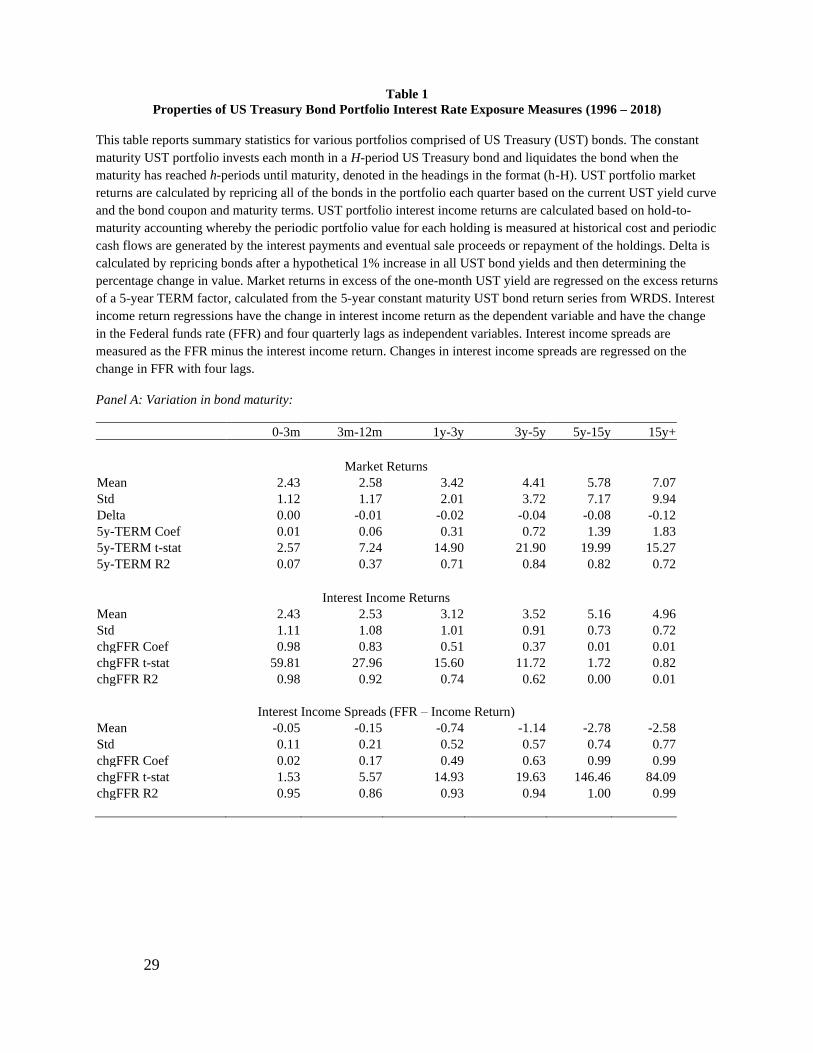
change in value. Panel A in Table 1 clearly shows that duration risk (Delta) is increasing in the

maturity of the portfolio. The value of portfolios with a maturity or repricing date of at least 15+

years falls by 12%, while the value of portfolios with a maturity between three months and 12

months falls by only 1% with an increase in the interest rate. Consistent with this conceptual

relation, when we regress the various UST portfolio market returns in excess of the one-month

UST yield on the excess returns of a 5-year TERM factor, calculated as the excess return of the

8

5-year constant maturity UST bond return series from WRDS, we find that the coefficient on the

5-year TERM factor increases with the maturity of the portfolio, consistent with a strong relation

between maturity and TERM risk exposure.

A reliable prediction from standard asset pricing theory is that higher risk exposures are

associated with a higher risk premium. Consistent with this prediction, UST portfolios with a

longer maturity earn a higher mean returns than UST portfolios of shorter maturity. The mean

market return of a UST portfolio with a maturity of less than three months is 2.43% per annum,

while a portfolio with a maturity of more than 15 years has earned 7.07% on average over our

sample period. As Fama (2006) emphasizes, TERM exposure has been a highly attractive risk

premium since 1981.

Interest rate sensitivity measures based on interest income returns suggest very different

properties of bond portfolio interest rate risk. Consistent with earning a higher risk premium,

longer maturity UST portfolios earn a higher mean income returns than shorter maturity bond

portfolios. Table 1 also shows that the volatility of interest income returns on UST portfolios

decreases with maturity. This counterfactually suggests a lower interest rate risk exposure of

portfolios with longer maturity. When we calculate interest rate risk exposures based on the

change in income returns regressed on the change in the Federal funds rate and four quarterly

lags, the coefficients decline with maturity of the UST portfolio. In addition, for portfolios with a

maturity of more than five-years, the explanatory power declines to zero.

The reason for this pattern is that the fixed income (i.e., the coupon payments) on these

portfolios sums coupons of bonds issued at different points in time. The longer the maturity, the

more coupons payments from different points in time are included in the sum and the resulting

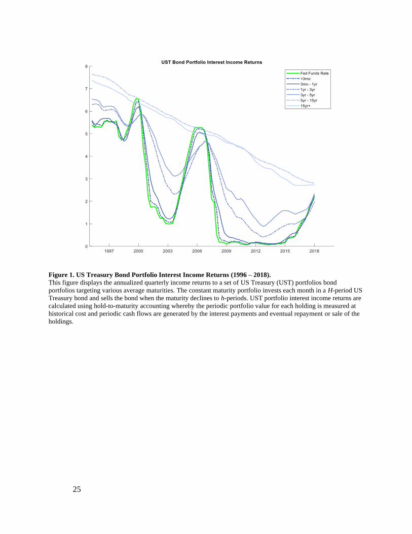
income time series is smoother than from a shorter maturity portfolio. Figure 1, which displays

the income return on different bond portfolios with various maturities, shows this clearly. The

9

longer the maturity of the portfolio the smoother the income return. This explains why a

regression of a long-maturity bond portfolio income return on changes in the Federal funds rate

will deliver a small coefficient and little explanatory power. Figure 1 also illustrates that the

mean income return tends to be increasing in portfolio maturity, which will provide the basis for

some future analyses.

Another version of the previous regression is based on the interest income spread, i.e., the

difference in the Federal funds rate and the income return. This version is more commonly used

in the recent literature (e.g., see DSS 2020) and measures the “sluggishness” in rate adjustments.2

The coefficients on the change in the Federal funds are equal to 1 minus the coefficient on the

equivalent regression coefficient in the income return regression discussed above. As a result, the

coefficients, also commonly called spread betas, are now increasing with the maturity and appear

to have high explanatory power. Note though that for long maturity UST portfolios, the variation

of the dependent variable is almost exclusively coming from the Federal funds rate, which also

shows up on the right-hand side of the regression as the explanatory variable, leading to a high

R2. Higher income spread coefficients (referred to as spread betas by DSS 2020) are interpreted

as these portfolios having higher “sluggishness” in rate adjustment in response to changes in

market rates. It is important to note that the artificial smoothing of interest income returns caused

by the increased maturity does not translate into lower duration risk, and of course, does not

reflect a managerial action to “sluggishly” adjust rates in response to changes in market rates.

To highlight the role of the cash share 𝜔𝑡, we vary the cash share from 0% to 100% for a

portfolio with its remaining share invested in UST bonds of maturities from three years to five

2 There is an earlier literature examining the empirical relation between deposit rates and market interest rates that

rely on income returns and income spreads (e.g. Ausbel (1990), Berger and Hannan (1989), Hannan and Berger

(1991), Hannan and Liang (1990), Neumark and Sharpe (1992), and Diebold and Sharpe (1990)).

10

years, results in Panel B of Table 1. Market returns and duration risk exposure, as measured by

both delta and the 5-year TERM coefficient, are declining as the cash share increases. The

average interest income return is also declining with the cash share, while its volatility is

increasing. Importantly, in regressions of the income return the coefficient on the change in the

Federal funds rate is increasing with the cash share, consistent with the premise that this

coefficient will be strongly related to the the share of (within a year with lags) zero-duration

assets in the portfolio. Equivalently, the income spread regressions have coefficients (i.e. spread

betas) that are decreasing in the cash share, which would commonly be interpreted as a decrease

in the sluggishness in rate adjustment to changes in market rates, despite these clearly being

passive portfolio strategies with no such intent.

These results demonstrate that a wide range of duration risks can be created across

portfolios that have different combinations of maturity and cash shares and that inferences about

these portfolio duration risk exposures will be difficult to identify with income or income spread

based measures.

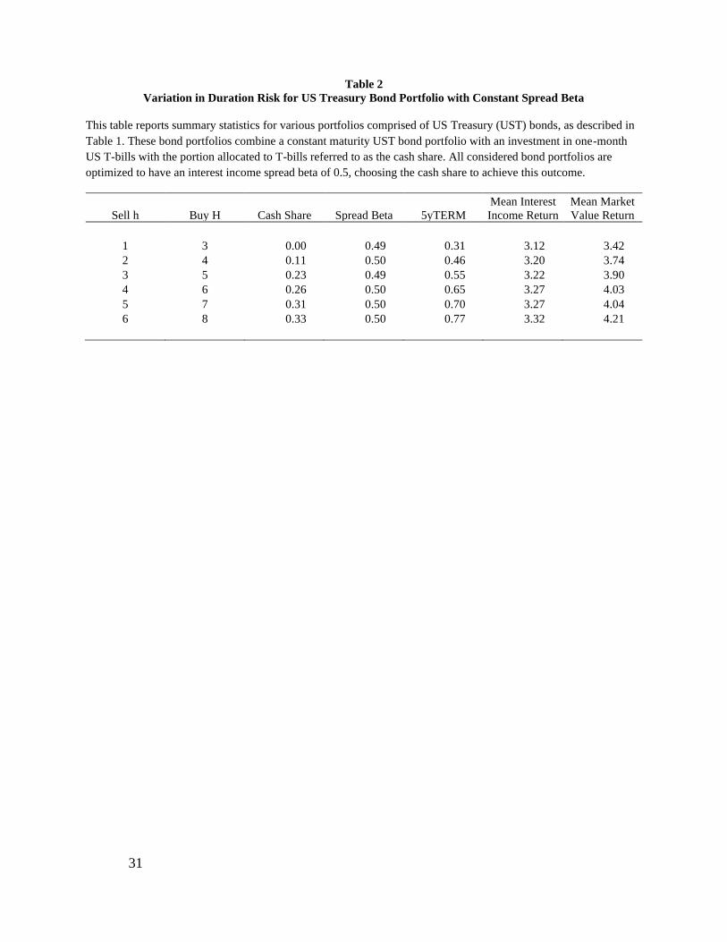
To illustrate how poorly identified duration risk is with income return based measures,

we consider six portfolios strategies that seek to increase their portfolio duration risk exposure,

while maintaining a target spread beta of 0.5, by investing in constant maturity UST bonds and

cash. Table 2 reports the results from this exercise. Table 2 shows that estimated spread betas are

essentially constant at their specified target of 0.5, while duration risk as measured by the

loading on the 5-year Term factor more than doubles from the lowest to the highest of the

considered strategies. To construct this table, we calculate bond portfolios that buy bonds at

maturity H and sell them when the remaining maturity goes to h. Moving down the rows of

Table 2, both the duration risk as measured by the 5-year TERM factor as well as the cash share

of the portfolio increases. Consistent with the portfolio duration risk exposure increasing across

11

these portfolios, the mean returns are also monotonically increasing across these portfolios. Yet

the spread beta coefficient remains constant, demonstrating that spread betas are not informative

about the extent of duration risk exposure.

To summarize, our UST bond analysis has shown that stable income streams generated

by fixed income portfolios do not easily reveal their duration risk exposure with methods that

provide the basis for the conclusion that banks do not bear interest rate risk. Thus, these

conclusions seem premature. Empirical measures of the “sluggishness” in the adjustment of

income returns to changes in market rates are strongly related to the maturity composition of

passive UST bond portfolios. In the next section we investigate how these measurement

properties affect inferences relying on bank data.

III. Properties of Interest Rate Risk Measures for Bank Activities

A. The Maturity Composition of Bank Activities and Spread Betas

Armed with the insights from our UST laboratory, we now turn to bank activities (i.e.,

loans, securities, deposits, and non-deposit borrowing) to investigate the extent to which the

sluggishness in bank income and expense rates to market rate movements can be explained by

the maturity composition of the activity. We begin with a summary of the maturity composition

of various bank activities.

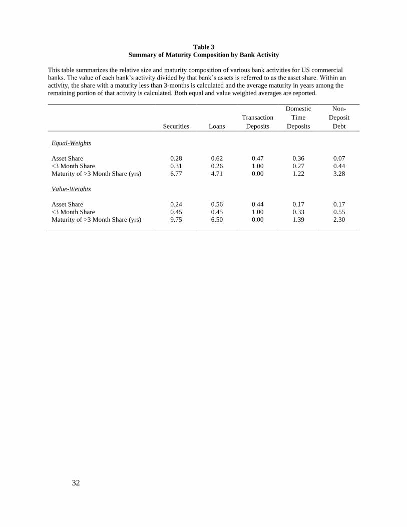
Table 3 summarizes the maturity composition and relative asset share by bank activity for

the equal weighted and value weighted sample of banks. We define securities as cash, Federal

funds and repo contracts sold, and securities. Table 3 shows that there is substantially more

cross-sectional variation in the maturity composition of assets (i.e., compare the less than 3-

month maturity or floating share of loans and security across the value weighted and equal

12

weighted rows) than on the liability side of banks most notably domestic time deposits and non-

deposit debt.

By both weighting schemes securities represent roughly a quarter of the balance sheet,

with 31% (equal-weighted) to 45% (value-weighted) invested in securities that mature or reprice

within a quarter. The average maturity for securities with longer maturity or repricing dates is

6.77 years (equal-weighted) or 9.75 years (value weighted). Loans represent slightly more than

half of the assets of banks, with a quarter (equal weighted) or 56% (value-weighted) invested in

contracts that reprice or mature within a quarter. The average maturity of all other loans is almost

4.71 years or 6.50 years for the equal weighted and value weighted sample, respectively.

Transaction deposits (i.e., demand and saving accounts) fund roughly 45% of bank assets.

Smaller banks have a larger domestic time deposit share (36%), while the value weighted sample

funds only 17% of assets with domestic time deposits. The maturity composition is fairly similar

across small and large banks, with around a third of time deposits maturing within a quarter and

the rest having a short maturity of a year and a quarter. Larger banks also use a significant

amount of non-deposit debt (17%) of which 55% matures within a quarter with the remaining

share having a maturity of 2.3 years. Except for transaction deposits, the maturity composition

for most other key balance sheet items can be easily discerned from bank data. In addition, Table

3 confirms the standard maturity transformation view of banks – banks invest in longer maturity

assets funded with shorter maturity liabilities.

We next investigate the extent to which the maturity composition of banks maps into the

commonly used interest rate spread betas to measure the degree of banks’ interest rate risk

exposure. We calculate interest rate spread betas as the literature (DSS, 2020) by taking the

difference between the quarterly Federal funds rate and the interest income or interest expense

rate on a bank activity and regressing the quarterly change of this variable on the quarterly

13

change in the Federal funds rate and four lags. The coefficients on the Federal funds rate and its

lags are summed to represent the interest rate spread beta.

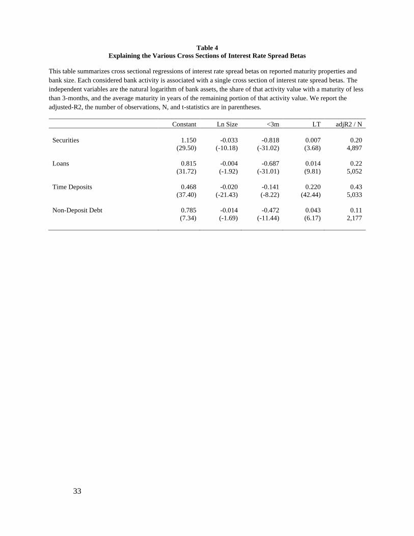
Table 4 presents cross-sectional regression results of interest rate spread betas on the

maturity composition of bank assets, controlling for bank size (ln assets). We describe the

maturity composition by the share of the bank activity that matures within a quarter and the

average maturity in years of the remaining portion. We find that this regression explains roughly

20% of the cross-sectional variation in interest rate spread betas of securities and loans; for

domestic time deposits it is nearly a half; while for non-deposit debt 11% of the variation is

explained. The coefficients on the short maturity share are large and negative across all activities.

This means that banks with a higher cash share in a specific activity tend to have lower spread

betas and therefore a higher sensitivity of the interest income / expense to changes in the Federal

funds rate. As demonstrated in the analysis in Section II, holding everything else equal a higher

cash share reduces duration risk. The coefficients on the average maturity are positive with large

t-statistics, consistent with the notion that spread betas are increasing in the average maturity of

the bank activity, as is the case in UST bond portfolios. These results indicate that

“sluggishness” in rate adjustments (as proxied by spread beta) are reliably linked to the maturity

composition of assets.

B. Market Power versus Maturity Composition

In this section, we investigate the link between market power and income spread betas.

Given the prominence of market power as an explanation for rate sluggishness, we examine how

much of the cross-sectional variation in spread betas is explained by market power proxies and

how much is explained by the reported maturity composition. We focus on securities and

deposits because the interest income and interest expense generated by these activities are free of

the confounding effects caused by credit risk premia. It is perhaps useful to note that the interest

14

income earned on a risky loan includes the ex ante risk premium, but not the ex post realizations

of credit-related losses. This highlights that the smoothness of the income return on a loan

portfolio surely does not appropriately indicate that the credit risk has been eliminated or hedged,

only that the time series variation in the interest income return does not reflect this risk exposure.

The mean risk premium (including the expected loss, which is not realized) will be reflected in

the mean interest income return.

There is a long literature that associates price rigidity in bank deposits with market power

(e.g., Berger and Hannan (1989), Hannan and Berger (1991), Neumark and Sharpe (1992),

Diebold and Sharpe (1990), Drechsler, Schnabl, and Savov (2017)). The primary evidence

supporting the view that banks have market power in their deposit-taking activity is that retail

deposit rates (1) tend to be lower than market rates and (2) adjust more slowly and less

completely to changes in market rates in more highly concentrated markets. There are two

variables that provide an empirical link to market power. The first is the Herfindahl-Hirschman

index (HHI) based on geographic deposit market concentration. The second is the deposit spread

beta, proposed by DSS 2017. We consider both of these measures.

In the first of these analyses, we sort banks by their market power proxies into groups of

low and high potential market power. According to the US Justice Department3, HHI values

below 1,500 are considered unconcentrated, values between 1,500 and 2,500 are moderately

concentrated, and values over 2,500 are highly concentrated. Based on these guidelines, we

define low market concentration as below 1,500 and high concentration above 2,500. When

classifying on the basis of transaction deposit spread betas, we define low market power as

below the 25th percentile and define high market power as above the 75th percentile.

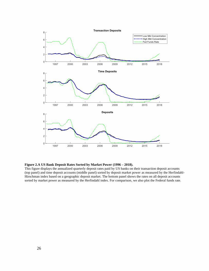
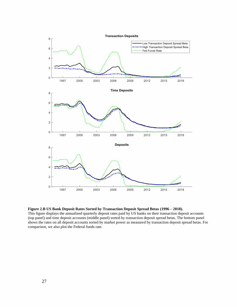
Figure 2 summarizes bank deposits rates for banks classified on the basis of their

potential market power using both of these proxies. The first panel of Figure 2 displays

3 https://www.justice.gov/atr/herfindahl-hirschman-

index#:~:text=The%20term%20%E2%80%9CHHI%E2%80%9D%20means%20the,then%20summing%20the%20r

esulting%20numbers.

15

transaction deposits, time deposits are plotted in the second panel, and total deposits are

displayed in the third panel. There are two important properties of deposits illustrated in Figure

2. First, comparing the time deposit rates with the transaction deposit rate shows that only

transaction deposits have the important marker of potential market power of paying below

market rates. Thus, we view the transaction deposit spread beta to be the relevant market power

proxy, rather than one based on total deposits. The second striking feature is that the direct link

to market concentration, as measured by HHI, appears to explain little of the cross sectional

variation in any of the deposit rates. Moreover, for time deposit rates neither market power proxy

appears to be meaningfully linked to the deposit rates.

We next explore the cross section of mean time deposit rates and the cross section of time

deposit spread betas in more detail with regression analysis. We study the mean of time deposits

because a higher duration risk exposure should show up in a higher average rate, everything else

equal. We also learned from Section II that spread betas are increasing in the maturity of the

bank activity and decreasing in the cash share, though not informative about the actual duration

exposure.

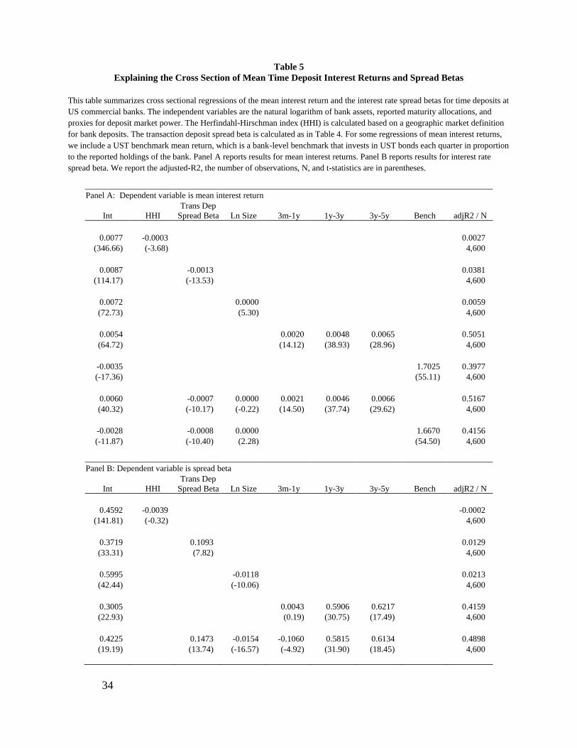
Table 5 summarizes the results of cross-sectional regressions that investigate how much

of the cross-sectional variation in average time deposit rates (Panel A) and time deposit spread

betas (Panel B) can be explained by cross-sectional variation in maturity composition and

proxies for market power. We use the two market power measures from the literature, the HHI

and the transaction deposit spread beta. The first two rows of Panel A show that the transaction

deposit spread beta is a more reliable predictor of mean time deposit rates than HHI.

Interestingly, market power whether measured by HHI or transaction deposit spread beta

explains very little of the cross-sectional variation in time deposit rate means. The R2s from

these regressions are very low, ranging from less than one percent in the case of HHI to about 4

percent in the case of transaction deposit spread betas. Bank size enters positively and

significantly, but also explains little of the cross-sectional variation in the time deposit rate.

16

We next explore how much of the mean in time deposits is explained by their maturity

composition. Recall from Table 3 that the cross-sectional variation in time deposit maturity is not

very large. Row 4 of Panel A shows that despite the relatively limited variation in maturity

composition of banks’ time deposits, the specification that includes only maturity composition

explains half of the variation in time deposit rate means. All maturity categories enter with a

positive sign and are highly statistically significant. In this regression, the omitted category is the

zero-duration asset share. Alternatively, we can also capture the cross-sectional difference in

maturity composition of time deposits with their benchmark return. The bank-level benchmark

return is the return on a portfolio of US Treasury bonds that invests in a set of constant maturity

UST portfolios in the same proportions as a bank’s time deposit maturity composition. In a

univariate regression, the mean benchmark income return explains 40% of the cross-sectional

variation with a highly significant coefficient. When we combine the strongest market power

measure, the transaction deposit spread beta, together with the maturity composition information

and control for size, the adjusted R2 goes up by only one percentage point (from 50.51% to

51.67%) relative to maturity composition alone. The coefficient on the transaction deposit spread

beta falls by a half, while the coefficient on the maturity buckets remain stable. Switching out the

maturity buckets for the benchmark return leads to a similar result. Most of the variation in the

time deposit rate mean is explained by its maturity composition. This suggests that the standard

asset pricing prediction of higher duration risk and therefore higher risk premia is highly

informative about explaining mean time deposit rates, and substantially more helpful in

explaining cross sectional variation than either of the two market power proxies.

Panel B reports results exploring how the “sluggishness” in time deposit rates can be

explained by market power and their maturity composition. The first two rows display the results

for market power alone. While the Herfindahl index alone is not statistically significant, the

coefficient on the transaction deposit spread beta is positive and highly significant. Nonetheless,

only 1.3% of the cross-sectional variation in time deposit spread betas is explained by this

measure of market power. Larger banks tend to have lower spread betas, meaning that they

17

reprice their deposits slightly more often than small banks. However, size explains only 2% of

the cross-sectional variation in deposit spread betas. In contrast, maturity composition explains

42% of the cross-sectional variation in the time deposit spread beta. Banks with a higher share in

time deposits that mature or reprice in more than one year tend to have higher (i.e., more

sluggish response) deposit spread betas. The coefficient on the three months to one-year maturity

share is near zero and insignificant, consistent with a change in the sign close to the omitted

category, the less than three-months maturity share. The regression of the time deposit spread

beta on the transaction deposit spread beta, size, and the time deposit maturity composition

explains 49% of the cross-sectional variation in time deposit spread betas, only an 8-percentage

point increase in explanatory power over maturity composition alone. Thus, in line with our

results from Section II, the maturity composition of time deposits explains a sizeable share of the

sluggishness in rate adjustments.

We now describe the analogue set of results for bank securities. We focus on securities to

investigate how much of the cross-sectional variation in means and spread betas can be explained

by the maturity composition because securities are generally free of other confounding risk

factors such as credit risk that may obfuscate the relationship between maturity composition and

the mean of rates and their sluggishness. Table 6 is structured in the same way as Table 5. In the

regressions of Panel A, the dependent variable is the mean interest rate, while in Panel B the

dependent variable is the spread beta. The results are also very similar. The two measures of

deposit market power are both significant and enter negatively but explain very little of the

cross-sectional variation in the mean interest rate. Size is more important for securities than for

time deposit means, alone explaining 11% of the variation. Larger banks earn a higher yield on

their securities than smaller banks. Maturity composition, as represented by the UST benchmark

return based on a bank’s securities maturity composition or the maturity composition directly,

explains 23% and 29%, respectively, of the variation in mean returns. A higher share of

securities in the 5 years and more category is especially reliably associated with increased mean

income returns on securities. Adding the transaction deposit spread beta and size to the maturity

18

composition regressions increases the adjusted R2 only by roughly 5 percentage points. When

we add size and market power to the benchmark return, the adjusted R2 increases by 2

percentage points.

In Panel B, the dependent variable is the spread beta of securities. Market power

measured either way is associated with higher securities spread betas, but the explanatory power

is small. The income return on securities of larger banks moves more with the market than the

income return on smaller banks, explaining little of the cross-sectional variation, even after

controlling for market power. Maturity composition, on the other hand, explains 20% of the

cross-sectional variation in the spread betas of securities. All larger than one-year maturity

categories enter with a statistically positive coefficient. Adding size and market power to the

maturity composition only increases the adjusted R2 by about 2 percentage points. As with time

deposits, the apparent sluggishness in the rate adjustments is more closely related to the maturity

composition of securities than with proxies for market power.

IV. Duration Risk Exposures with Stable Net Interest Margin

An important bank performance measure is the net interest margin (NIM), calculated as

the net of interest income minus interest expense, divided by assets. Many banks acknowledge

that they explicitly target a stable time series NIM. For example, the 2019 annual report for

Ameris Bankcorp states, “The goal of the Company’s interest rate risk management process is to

minimize the volatility in the net interest margin caused by changes in interest rates.” Almost all

US commercial banks do have highly stable NIM. For the 4,048 US commercial banks with a

full time series of quarterly NIM over the period 1996 through 2018, we calculate the standard

deviation of quarterly NIM for each bank. The 95th percentile of annualized NIM volatility is

0.55%, while the annualized volatility for the Federal funds rate is 1.12%. The remarkable time

series stability of net interest margin is sometimes interpreted as evidence that banks have

19

hedged their interest rate exposure by practitioners and academic researchers alike (e.g.

Drechsler, Savov, and Schnabl (2020), (DSS 2020)).4

Drechsler, Savov, and Schnabl (2020) “show that maturity transformation does not

expose banks to interest rate risk—it hedges it. The reason is the deposit franchise, which allows

banks to pay deposit rates that are low and insensitive to market interest rates. Hedging the

deposit franchise requires banks to earn income that is also insensitive, i.e. to lend long-term at

fixed rates.” The key to this hedging strategy is that the net of interest income and interest

expense is insensitive to market interest rates. However, such a hedging strategy may do little to

eliminate the duration risk to bond value associated with discount rate shocks that one expects

from lending long-term at fixed rates. We investigate this possibility in this section.

To explore the potential for duration risk to coexist with a bond portfolio exhibiting

stable NIM, we focus on a type of narrow bank that only invests in securities and issues time

deposits. This allows us to study actual bank data since these are a subset of the bank business

model with detailed reported maturity data and to isolate the effects of duration risk since these

activities are relatively free of the confounding effects caused by credit risk premia. For each

bank, we also construct a narrow NIM benchmark using the bank-level securities and time

deposit UST benchmarks that invest in constant maturity UST bond portfolios according to the

reported maturity allocations. We first document that narrow NIM has the desirable properties of

the full NIM. Specifically, narrow NIM is highly stable through time for virtually all banks and

there is a strong tendency for the time deposit spread betas and the securities spread betas to be

offsetting at the bank-level. We then test whether there is predictability in the cross sectional

narrow NIM mean using benchmarks that invest in UST bonds according to the reported

maturity distributions. To the extent that narrow NIM represents well-hedged portfolios with

4 For example, the 2018 annual report of Bank of America states “interest rate risk represents the most significant

market risk exposure to our banking book balance sheet. Interest rate risk is measured as the potential change in net

interest income caused by movements in market interest rates.”

20

respect to interest rate risks, there should be no predictability related to the reported maturity

exposure.

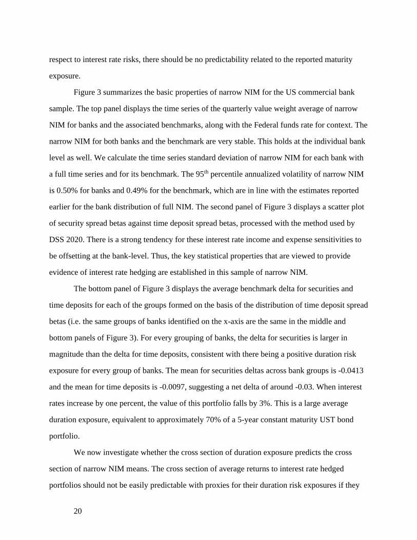
Figure 3 summarizes the basic properties of narrow NIM for the US commercial bank

sample. The top panel displays the time series of the quarterly value weight average of narrow

NIM for banks and the associated benchmarks, along with the Federal funds rate for context. The

narrow NIM for both banks and the benchmark are very stable. This holds at the individual bank

level as well. We calculate the time series standard deviation of narrow NIM for each bank with

a full time series and for its benchmark. The 95th percentile annualized volatility of narrow NIM

is 0.50% for banks and 0.49% for the benchmark, which are in line with the estimates reported

earlier for the bank distribution of full NIM. The second panel of Figure 3 displays a scatter plot

of security spread betas against time deposit spread betas, processed with the method used by

DSS 2020. There is a strong tendency for these interest rate income and expense sensitivities to

be offsetting at the bank-level. Thus, the key statistical properties that are viewed to provide

evidence of interest rate hedging are established in this sample of narrow NIM.

The bottom panel of Figure 3 displays the average benchmark delta for securities and

time deposits for each of the groups formed on the basis of the distribution of time deposit spread

betas (i.e. the same groups of banks identified on the x-axis are the same in the middle and

bottom panels of Figure 3). For every grouping of banks, the delta for securities is larger in

magnitude than the delta for time deposits, consistent with there being a positive duration risk

exposure for every group of banks. The mean for securities deltas across bank groups is -0.0413

and the mean for time deposits is -0.0097, suggesting a net delta of around -0.03. When interest

rates increase by one percent, the value of this portfolio falls by 3%. This is a large average

duration exposure, equivalent to approximately 70% of a 5-year constant maturity UST bond

portfolio.

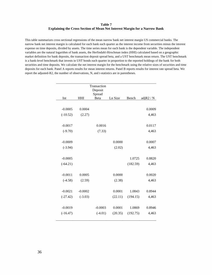
We now investigate whether the cross section of duration exposure predicts the cross

section of narrow NIM means. The cross section of average returns to interest rate hedged

portfolios should not be easily predictable with proxies for their duration risk exposures if they

21

are in fact well-hedged. However, if the duration risk has not been hedged, then there may be a

positive relation in narrow NIM mean and predicted mean based on maturity composition. Table

7 reports results from cross sectional regressions of the time series mean of narrow NIM for

banks on bank characteristics like market power proxies, bank size, as well as the mean narrow

NIM benchmark for each bank. The key variable is the mean benchmark, which is constructed

based on the reported maturity allocations of securities and time deposits for each bank. In a

univariate regression, the coefficient on the benchmark mean is 1.07 (t-statistic = 183) with an

R2 of 0.88. In specifications that include other variables, the coefficient on the benchmark is

essentially unchanged and the adjusted R2 is minimally affected. Interestingly, the coefficients

on the two proxies for market power (HHI and the transaction deposit spread beta) explain little

of the cross sectional variation in narrow NIM mean with associated R2 estimates below 0.02 in

univariate regressions and have reliably negative coefficients in specifications that include the

benchmark mean return. These results indicate that there is a highly reliable relation between the

narrow NIM mean and the predicted mean proxied by the mean of passive maturity-matched

benchmarks, highlighting the existence of substantial duration risk in portfolios exhibiting highly

stable NIM and asset-liability interest spread beta matching.

V. Conclusion

This paper reexamines the reliability of empirical methods used to conclude that banks do

not bear interest rate risk. The specific concern is that duration risk – a repricing risk caused by

changing interest rates that affects prices or values and that commands large risk premia in

capital markets over the past 40 years – will not be well identified from methods that estimate

the time series sensitivities of interest income returns (i.e. interest income scaled by par or book

value). We demonstrate that this concern is warranted.

The attempt to use NIM to investigate banks' interest rate risk exposure reveals a

common misconception related to banks' risk exposure, namely the notion that risk should reveal

itself in income or expense rates. We demonstrate that the stability of interest income and

22

expense rates, and therefore NIM, are not informative about duration risk and show that the

mean income return across portfolios that have their interest income sensitivities hedged by their

interest expense sensitivities are highly predictable by their duration risk exposure. The

inconsistent recognition of duration risk as a component of interest rate risk reconciles the two

views about banks' interest rate exposures.

23

References

Begenau, Juliane, Monika Piazzesi, Martin Schneider, 2015. Banks’ Risk Exposure. Stanford

working paper.

Berger, Allen N., and Timothy H. Hannan. "The price-concentration relationship in banking."

The Review of Economics and Statistics (1989): 291-299.

Diebold, Francis X., and Steven A. Sharpe. "Post-deregulation bank-deposit-rate pricing: The

multivariate dynamics." Journal of Business & Economic Statistics 8, no. 3 (1990): 281-

291.

Drechsler, I., Savov, A. and Schnabl, P., 2017. The deposits channel of monetary policy. The

Quarterly Journal of Economics, 132(4), pp.1819-1876.

Drechsler, I, Savov, A. and Schnabl, P., 2018. Banking on Deposits: Maturity Transformation

without Interest Rate Risk, working paper.

English, W.B., Van den Heuvel, S.J. and Zakrajšek, E., 2018. Interest rate risk and bank equity

valuations. Journal of Monetary Economics, 98, pp.80-97.

Fama, Eugene F, 1985. What’s Different about Banks? Journal of Monetary Economics 15, 29-

39.

Fama, Eugene F, 2006. The Behavior of Interest Rates. The Review of Financial Studies 19, no.

2, 359-379.

Flannery, M.J. and James, C.M., 1984. The effect of interest rate changes on the common stock

returns of financial institutions. The Journal of Finance, 39(4), pp.1141-1153.

Flannery, M.J. and James, C.M., 1984. Market evidence on the effective maturity of bank assets

and liabilities. Journal of Money, Credit and Banking, 16(4), pp.435-445.

Gomez, M., Landier, A., Sraer, D.A. and Thesmar, D., 2019. Banks' exposure to interest rate risk

and the transmission of monetary policy. MIT working paper.

Gorton, G., and G. Pennacchi, 1990. Financial intermediaries and liquidity creation. The Journal

of Finance, 45, pp. 49–71.

Han, J., Park, K. and Pennacchi, G., 2015. Corporate taxes and securitization. The Journal of

Finance, 70(3), pp.1287-1321.

Hannan, T., and A. Berger. "The Rigidity of Prices: Evidence from the Banking Industry."

American Economic Review, 81 (1991), 93

Hutchison, D.E. and Pennacchi, G.G., 1996. Measuring rents and interest rate risk in imperfect

financial markets: The case of retail bank deposits. Journal of Financial and Quantitative

Analysis, pp.399-417.

24

Krishnamurthy, Arvind, and Annette Vissing-Jorgensen. The aggregate demand for treasury

debt. Journal of Political Economy 120, no. 2 (2012): 233-267.

Neumark, David, and Steven A. Sharpe. "Market structure and the nature of price rigidity:

evidence from the market for consumer deposits." The Quarterly Journal of Economics

107, no. 2 (1992): 657-680.

25

Figure 1. US Treasury Bond Portfolio Interest Income Returns (1996 – 2018).

This figure displays the annualized quarterly income returns to a set of US Treasury (UST) portfolios bond

portfolios targeting various average maturities. The constant maturity portfolio invests each month in a H-period US

Treasury bond and sells the bond when the maturity declines to h-periods. UST portfolio interest income returns are

calculated using hold-to-maturity accounting whereby the periodic portfolio value for each holding is measured at

historical cost and periodic cash flows are generated by the interest payments and eventual repayment or sale of the

holdings.

26

Figure 2.A US Bank Deposit Rates Sorted by Market Power (1996 – 2018).

This figure displays the annualized quarterly deposit rates paid by US banks on their transaction deposit accounts

(top panel) and time deposit accounts (middle panel) sorted by deposit market power as measured by the Herfindahl-

Hirschman index based on a geographic deposit market. The bottom panel shows the rates on all deposit accounts

sorted by market power as measured by the Herfindahl index. For comparison, we also plot the Federal funds rate.

27

Figure 2.B US Bank Deposit Rates Sorted by Transaction Deposit Spread Betas (1996 – 2018).

This figure displays the annualized quarterly deposit rates paid by US banks on their transaction deposit accounts

(top panel) and time deposit accounts (middle panel) sorted by transaction deposit spread betas. The bottom panel

shows the rates on all deposit accounts sorted by market power as measured by transaction deposit spread betas. For

comparison, we also plot the Federal funds rate.

28

Figure 3. Net Interest Margin for a Narrow Bank.

This figure summarizes the properties of the annualized quarterly net interest margin (NIM), calculated from bank

securities interest income minus time deposit interest expense, divided by assets. Panel A displays the time series

NIM for banks and a US Treasury (UST) benchmark, which is the value weight average of bank-level benchmarks

calculated for securities and time deposits based on reported maturities. For comparison, we also plot the Federal

funds rate. Panel B displays a scatter plot of securities spread betas against time deposit spread betas. Spread betas

are calculated via regressions of changes in the Federal funds rate (FFR) minus the interest income (expense) return

on changes in the FFR and four lags of the changes in FFR. We form 50 equally sized bins based on the distribution

of time deposit spread betas and calculate the average spread beta within each bin. Panel C displays the average

duration risk as measured by the benchmark delta for securities and time deposits for the groups of banks formed by

the process defined in Panel B.

29

Table 1

Properties of US Treasury Bond Portfolio Interest Rate Exposure Measures (1996 – 2018)

This table reports summary statistics for various portfolios comprised of US Treasury (UST) bonds. The constant

maturity UST portfolio invests each month in a H-period US Treasury bond and liquidates the bond when the

maturity has reached h-periods until maturity, denoted in the headings in the format (h-H). UST portfolio market

returns are calculated by repricing all of the bonds in the portfolio each quarter based on the current UST yield curve

and the bond coupon and maturity terms. UST portfolio interest income returns are calculated based on hold-to-

maturity accounting whereby the periodic portfolio value for each holding is measured at historical cost and periodic

cash flows are generated by the interest payments and eventual sale proceeds or repayment of the holdings. Delta is

calculated by repricing bonds after a hypothetical 1% increase in all UST bond yields and then determining the

percentage change in value. Market returns in excess of the one-month UST yield are regressed on the excess returns

of a 5-year TERM factor, calculated from the 5-year constant maturity UST bond return series from WRDS. Interest

income return regressions have the change in interest income return as the dependent variable and have the change

in the Federal funds rate (FFR) and four quarterly lags as independent variables. Interest income spreads are

measured as the FFR minus the interest income return. Changes in interest income spreads are regressed on the

change in FFR with four lags.

Panel A: Variation in bond maturity:

0-3m 3m-12m 1y-3y 3y-5y 5y-15y 15y+

Market Returns

Mean 2.43 2.58 3.42 4.41 5.78 7.07

Std 1.12 1.17 2.01 3.72 7.17 9.94

Delta 0.00 -0.01 -0.02 -0.04 -0.08 -0.12

5y-TERM Coef 0.01 0.06 0.31 0.72 1.39 1.83

5y-TERM t-stat 2.57 7.24 14.90 21.90 19.99 15.27

5y-TERM R2 0.07 0.37 0.71 0.84 0.82 0.72

Interest Income Returns

Mean 2.43 2.53 3.12 3.52 5.16 4.96

Std 1.11 1.08 1.01 0.91 0.73 0.72

chgFFR Coef 0.98 0.83 0.51 0.37 0.01 0.01

chgFFR t-stat 59.81 27.96 15.60 11.72 1.72 0.82

chgFFR R2 0.98 0.92 0.74 0.62 0.00 0.01

Interest Income Spreads (FFR – Income Return)

Mean -0.05 -0.15 -0.74 -1.14 -2.78 -2.58

Std 0.11 0.21 0.52 0.57 0.74 0.77

chgFFR Coef 0.02 0.17 0.49 0.63 0.99 0.99

chgFFR t-stat 1.53 5.57 14.93 19.63 146.46 84.09

chgFFR R2 0.95 0.86 0.93 0.94 1.00 0.99

30

Table 1 (continued)

Panel B: Variation in cash share for 3y-5y bond portfolio strategy:

0% 20% 40% 60% 80% 100%

Market Returns

Mean 4.41 3.97 3.52 3.08 2.63 2.38

Std 3.72 3.04 2.37 1.76 1.26 1.12

Delta -0.04 -0.03 -0.02 -0.01 -0.01 0.00

5y-TERM Coef 0.72 0.57 0.43 0.29 0.14 0.00

5y-TERM t-stat 21.90 21.83 21.74 21.61 21.53 0.27

5y-TERM R2 0.84 0.84 0.84 0.84 0.84 0.00

Interest Income Returns

Mean 3.52 3.26 2.99 2.72 2.45 2.38

Std 0.91 0.92 0.94 0.97 1.01 1.12

chgFFR Coef 0.37 0.49 0.60 0.72 0.84 1.00

chgFFR t-stat 11.72 17.18 18.46 16.98 15.25 n.a.

chgFFR R2 0.62 0.77 0.82 0.82 0.81 1.00

Interest Income Spreads (FFR – Income Return)

Mean -1.14 -0.87 -0.60 -0.34 -0.06 0.00

Std 0.57 0.46 0.36 0.26 0.17 0.00

chgFFR Coef 0.63 0.51 0.40 0.28 0.16 0.00

chgFFR t-stat 19.63 18.00 12.13 6.63 3.01 n.a.

chgFFR R2 0.94 0.93 0.85 0.62 0.26 n.a.

31

Table 2

Variation in Duration Risk for US Treasury Bond Portfolio with Constant Spread Beta

This table reports summary statistics for various portfolios comprised of US Treasury (UST) bonds, as described in

Table 1. These bond portfolios combine a constant maturity UST bond portfolio with an investment in one-month

US T-bills with the portion allocated to T-bills referred to as the cash share. All considered bond portfolios are

optimized to have an interest income spread beta of 0.5, choosing the cash share to achieve this outcome.

Sell h Buy H Cash Share Spread Beta 5yTERM

Mean Interest

Income Return

Mean Market

Value Return

1 3 0.00 0.49 0.31 3.12 3.42

2 4 0.11 0.50 0.46 3.20 3.74

3 5 0.23 0.49 0.55 3.22 3.90

4 6 0.26 0.50 0.65 3.27 4.03

5 7 0.31 0.50 0.70 3.27 4.04

6 8 0.33 0.50 0.77 3.32 4.21

32

Table 3

Summary of Maturity Composition by Bank Activity

This table summarizes the relative size and maturity composition of various bank activities for US commercial

banks. The value of each bank’s activity divided by that bank’s assets is referred to as the asset share. Within an

activity, the share with a maturity less than 3-months is calculated and the average maturity in years among the

remaining portion of that activity is calculated. Both equal and value weighted averages are reported.

Securities Loans

Transaction

Deposits

Domestic

Time

Deposits

Non-

Deposit

Debt

Equal-Weights

Asset Share 0.28 0.62 0.47 0.36 0.07

<3 Month Share 0.31 0.26 1.00 0.27 0.44

Maturity of >3 Month Share (yrs) 6.77 4.71 0.00 1.22 3.28

Value-Weights

Asset Share 0.24 0.56 0.44 0.17 0.17

<3 Month Share 0.45 0.45 1.00 0.33 0.55

Maturity of >3 Month Share (yrs) 9.75 6.50 0.00 1.39 2.30

33

Table 4

Explaining the Various Cross Sections of Interest Rate Spread Betas

This table summarizes cross sectional regressions of interest rate spread betas on reported maturity properties and

bank size. Each considered bank activity is associated with a single cross section of interest rate spread betas. The

independent variables are the natural logarithm of bank assets, the share of that activity value with a maturity of less

than 3-months, and the average maturity in years of the remaining portion of that activity value. We report the

adjusted-R2, the number of observations, N, and t-statistics are in parentheses.

Constant Ln Size <3m LT adjR2 / N

Securities 1.150 -0.033 -0.818 0.007 0.20

(29.50) (-10.18) (-31.02) (3.68) 4,897

Loans 0.815 -0.004 -0.687 0.014 0.22

(31.72) (-1.92) (-31.01) (9.81) 5,052

Time Deposits 0.468 -0.020 -0.141 0.220 0.43

(37.40) (-21.43) (-8.22) (42.44) 5,033

Non-Deposit Debt 0.785 -0.014 -0.472 0.043 0.11

(7.34) (-1.69) (-11.44) (6.17) 2,177

34

Table 5

Explaining the Cross Section of Mean Time Deposit Interest Returns and Spread Betas

This table summarizes cross sectional regressions of the mean interest return and the interest rate spread betas for time deposits at

US commercial banks. The independent variables are the natural logarithm of bank assets, reported maturity allocations, and

proxies for deposit market power. The Herfindahl-Hirschman index (HHI) is calculated based on a geographic market definition

for bank deposits. The transaction deposit spread beta is calculated as in Table 4. For some regressions of mean interest returns,

we include a UST benchmark mean return, which is a bank-level benchmark that invests in UST bonds each quarter in proportion

to the reported holdings of the bank. Panel A reports results for mean interest returns. Panel B reports results for interest rate

spread beta. We report the adjusted-R2, the number of observations, N, and t-statistics are in parentheses.

Panel A: Dependent variable is mean interest return

Int HHI

Trans Dep

Spread Beta Ln Size 3m-1y 1y-3y 3y-5y Bench adjR2 / N

0.0077 -0.0003 0.0027

(346.66) (-3.68) 4,600

0.0087 -0.0013 0.0381

(114.17) (-13.53) 4,600

0.0072 0.0000 0.0059

(72.73) (5.30) 4,600

0.0054 0.0020 0.0048 0.0065 0.5051

(64.72) (14.12) (38.93) (28.96) 4,600

-0.0035 1.7025 0.3977

(-17.36) (55.11) 4,600

0.0060 -0.0007 0.0000 0.0021 0.0046 0.0066 0.5167

(40.32) (-10.17) (-0.22) (14.50) (37.74) (29.62) 4,600

-0.0028 -0.0008 0.0000 1.6670 0.4156

(-11.87) (-10.40) (2.28) (54.50) 4,600

Panel B: Dependent variable is spread beta

Int HHI

Trans Dep

Spread Beta Ln Size 3m-1y 1y-3y 3y-5y Bench adjR2 / N

0.4592 -0.0039 -0.0002

(141.81) (-0.32) 4,600

0.3719 0.1093 0.0129

(33.31) (7.82) 4,600

0.5995 -0.0118 0.0213

(42.44) (-10.06) 4,600

0.3005 0.0043 0.5906 0.6217 0.4159

(22.93) (0.19) (30.75) (17.49) 4,600

0.4225 0.1473 -0.0154 -0.1060 0.5815 0.6134 0.4898

(19.19) (13.74) (-16.57) (-4.92) (31.90) (18.45) 4,600

35

Table 6

Explaining the Cross Section of Mean Securities Interest Returns and Spread Betas

This table summarizes cross sectional regressions of the mean interest return and the interest rate spread betas for securities at US

commercial banks. The independent variables are the natural logarithm of bank assets, reported maturity allocations, and proxies

for deposit market power. The Herfindahl-Hirschman index (HHI) is calculated based on a geographic market definition for bank

deposits. The transaction deposit spread beta is calculated as in Table 4. For some regressions of mean interest returns, we

include a UST benchmark mean return, which is a bank-level benchmark that invests in UST bonds each quarter in proportion to

the reported holdings of the bank. Panel A reports results for mean interest returns. Panel B reports results for interest rate spread

beta. We report the adjusted-R2, the number of observations, N, and t-statistics are in parentheses.

Panel A: Dependent variable is mean interest return

Int HHI

Trans Dep

Spread Beta Ln Size 3m-1y 1y-3y 3y-5y 5-15y 15y + Bench adjR2 / N

0.0105 -0.0008 0.0014

(139.28) (-2.66) 4,468

0.0129 -0.0033 0.0223

(49.68) (-10.13) 4,468

0.0031 0.0006 0.1062

(10.05) (23.05) 4,468

0.0019 0.9265 0.2325

(8.23) (36.80) 4,468

0.0079 0.0011 -0.0001 0.0017 0.0047 0.0103 0.2873

(48.75) (1.18) (-0.08) (2.34) (16.65) (24.67) 4,468

0.0058 -0.0021 0.0003 0.0009 -0.0001 0.0019 0.0048 0.0089 0.3350

(13.01) (-7.35) (12.96) (1.01) (-0.15) (2.79) (17.44) (21.22) 4,468

-0.0012 -0.0020 0.0004 0.8701 0.3075

(-2.54) (-6.79) (17.45) (35.88) 4,468

Panel B: Dependent variable is spread beta

Int HHI

Trans Dep

Spread Beta Ln Size 3m-1y 1y-3y 3y-5y 5y-15y 15y + Bench adjR2 / N

0.5630 0.0803 0.0009

(59.59) (2.24) 4,468

0.1897 0.4953 0.0320

(5.84) (12.19) 4,468

0.8170 -0.0197 0.0071

(19.75) (-5.72) 4,468

0.2858 0.0228 0.4664 -0.0066 0.0324

(4.46) (0.64) (10.81) (-1.81) 4,468

0.0283 0.2307 0.7479 1.0336 0.8237 0.6502 0.1952

(1.31) (1.87) (8.44) (10.75) (21.89) (11.62) 4,468

-0.0315 0.3649 -0.0192 0.2362 0.7526 0.9980 0.8117 0.7444 0.2256

(-0.52) (9.43) (-5.69) (1.95) (8.66) (10.58) (21.98) (13.12) 4,468

36

Table 7

Explaining the Cross Section of Mean Net Interest Margin for a Narrow Bank

This table summarizes cross sectional regressions of the mean narrow bank net interest margin US commercial banks. The

narrow bank net interest margin is calculated for each bank each quarter as the interest income from securities minus the interest

expense on time deposits, divided by assets. The time series mean for each bank is the dependent variable. The independent

variables are the natural logarithm of bank assets, the Herfindahl-Hirschman index (HHI) calculated based on a geographic

market definition for bank deposits, the transaction deposit spread beta, and a UST benchmark mean return. The UST benchmark

is a bank-level benchmark that invests in UST bonds each quarter in proportion to the reported holdings of the bank for both

securities and time deposits. We calculate the net interest margin for the benchmark using the relative sizes of securities and time

deposits for each bank. Panel A reports results for mean interest returns. Panel B reports results for interest rate spread beta. We

report the adjusted-R2, the number of observations, N, and t-statistics are in parentheses.

Int HHI

Transaction

Deposit

Spread

Beta Ln Size Bench adjR2 / N

-0.0005 0.0004 0.0009

(-10.52) (2.27) 4,463

-0.0017 0.0016 0.0117

(-9.70) (7.33) 4,463

-0.0009 0.0000 0.0007

(-3.94) (2.02) 4,463

-0.0005 1.0725 0.8820

(-64.21) (182.59) 4,463

-0.0011 0.0005 0.0000 0.0020

(-4.58) (2.59) (2.38) 4,463

-0.0021 -0.0002 0.0001 1.0843 0.8944

(-27.42) (-3.03) (22.11) (194.15) 4,463

-0.0019 -0.0003 0.0001 1.0869 0.8946

(-16.47) (-4.01) (20.35) (192.75) 4,463

37

Appendix

A.