staff scheduling problem thesis final
DESCRIPTION
Math Programming, student work, Thesis, model and applicationTRANSCRIPT

The staff scheduling problem: a general
model and applications
Marta Soares Ferreira da Silva Rocha
A Thesis submitted to Faculdade de Engenharia da Universidade do Portofor the doctoral degree in Industrial Engineering and Management
Supervisors
Professor Jose Fernando da Costa OliveiraProfessor Maria Antonia da Silva Lopes de Carravilla
Faculdade de Engenharia da Universidade do Porto
2013

Abstract
The scheduling of employees is a complex and time-consuming task. It iscomplex because it involves assigning the right people to the right job atthe right time. It is conditioned by several legal, work and other organi-zational rules. And it often copes with conflicting objectives, such as theminimization of the labor costs or the workforce size and the satisfaction ofthe employees preferences, for example. It is time-consuming because it isa periodic task and it is still manually performed in most organizations.
The research work described in this thesis deals with the development ofmethods for the automatic scheduling of employees, in particular for theirsimultaneous assignment to working shifts and days-off. The work focuseson the design of a general integer programming (IP) model that, followingan optimization approach, can be easily adapted and solve a wide set ofdifferent real-world problems. An innovative formulation of the sequence andconsecutiveness constraints gives the model the flexibility to accommodatevariable features of the problems. A cyclic approach ensures the generationof equitable and predictable work schedules.
The application of the general model is illustrated with three real-worldcase studies and a collection of benchmark instances available in the lit-erature. Computational results demonstrate the good performance of themodel, achieving optimal solutions for the majority of the problems in usefultime.
A constructive heuristic is also developed for solving one of the case-studies.Based on a set of simple calculations, the proposed procedure reveals tobe an efficient alternative to the IP optimization approach for solving thepractical problem considered. The good performance achieved with tests ona set of larger computer generated instances confirms the robustness of thisapproximate approach.
Although its apparent pertinency to the activity sector, staff schedulingproblems in hospitality management have been quite unnoticed by the re-search community. This thesis dedicates a chapter to this topic, namely tothe assessment of the potential of hospitality management as an applicationarea for staff scheduling problems and of possible resolution approaches.
i

ii

Resumo
O escalonamento de pessoal e uma tarefa complexa e fortemente consumi-dora de recursos. E complexa porque envolve a afetacao das pessoas certasao trabalho certo no momento certo. E condicionada por diversas regras denatureza legal, laboral ou organizacional. Lida normalmente com objetivosdivergentes, tais como a mimimizacao de custos ou a dimensao da equipade trabalho e a satisfacao das preferencias dos trabalhadores, por exemplo.Consome recursos porque e feita periodicamente e ainda de modo manual,em muitas organizacoes.
O trabalho de investigacao descrito nesta tese aborda o desenvolvimento demetodos para o escalonamento automatico de pessoal, em particular com asua afetacao simultanea a turnos de trabalho e dias de descanso. O trabalhocentra-se no desenvolvimento de um modelo geral de programacao inteiraque, seguindo uma abordagem de otimizacao, pode ser facilmente adaptadoe resolver um conjunto alargado de diferentes problemas reais. A formulacaoinovadora das restricoes de sequencia e consecutividade confere ao modeloa flexibilidade necessaria para acomodar caracterısticas variaveis dos prob-lemas. Uma abordagem cıclica assegura a geracao de horarios equilibradose previsıveis.
A aplicacao do modelo geral e ilustrada atraves de tres casos de estudobaseados em problemas reais e de um conjunto de instancias de benchmarkdisponıveis na literatura. Os resultados computacionais demonstram o bomdesempenho do modelo, obtendo as solucoes otimas para a maior parte dosproblemas em tempo util.
Uma heurıstica construtiva foi tambem desenvolvida para um dos casos deestudo. Baseado num conjunto de calculos simples, o procedimento pro-posto revela ser uma alternativa eficiente a abordagem de otimizacao para aresolucao do problema pratico considerado. O bom desempenho conseguidocom testes em instancias de maior dimensao comprova a robustez destemetodo aproximado.
Apesar da sua aparente pertinencia para o sector de atividade, os proble-mas de escalonamento de pessoal na area de gestao da hospitalidade naotem merecido a devida atencao por parte da comunidade academica. Estatese dedica um dos seus capıtulos a este topico, nomeadamente a avaliacaodo potencial da gestao da hospitalidade como uma area de aplicacao paraos problemas de escalonamento de pessoal e de possıveis abordagens de res-olucao.
iii

iv

Acknowledgments
This thesis is the culmination of the work accomplished during the mostdemanding phase of my personal life. During these four years, I felt myphysical and emotional endurance being strained to the limit. If I succeededand reached this far I owe it to the people that supported me in this journey,to whom I here address my sincere acknowledgments.
First of all, I would like to thank my supervisors, Jose Fernando Oliveiraand Maria Antonia Carravilla, for trusting me this exceptional opportunityto redirect the course of my career. It was a privilege to be part of yourresearch group but also to be part of your teaching group. I can now knowhow it feels to be on the other side of the classroom desk. It was a reallyenriching experience that allowed me to develop new competences. Thankyou for keeping me always focused and motivated. Thank you for yourdedication. Thank you for caring.
My second acknowledgment goes to all the colleagues from the IO Lab. Somehave already left. Some have just arrived. Others come and go. Others arethere to stay. Although I missed a lot of lunches, dinner parties and eveningouts, I really enjoyed the company of every one of you. Thank you for yourunderstanding and caring.
I must also thank Miguel Gomes, my “Mac adviser”, for his availability andhelp.
A heartfelt thanks to Vera, with whom I shared this path since the first day.You have been an outstanding friend. Thank you for all the coffees, all thetalks, all the help. Thank you for being always there.
I thank my parents, brother and in-laws for giving me the necessary condi-tions to carry out this project, especially during these last 1,5 years. Thankyou for your unconditional support.
I dedicate this thesis to Andre, Matilde and Beatriz. Thank you for yourinfinite love.
v

vi
Table of Contents
Abstract i
Resumo iii
Acknowledgements v
Table of Contents vii
List of Figures x
List of Tables xiv
1 Introduction 1
1.1 Motivation . . . . . . . . . . . . . . . . . . . . . . . . . . . . 1
1.2 Research approach . . . . . . . . . . . . . . . . . . . . . . . . 3
1.3 Thesis outline . . . . . . . . . . . . . . . . . . . . . . . . . . . 5
2 Staff scheduling problems 7
2.1 Defining the problem . . . . . . . . . . . . . . . . . . . . . . . 7
2.2 Modeling the problem . . . . . . . . . . . . . . . . . . . . . . 14
2.3 Reviewing related works in the literature . . . . . . . . . . . . 20
2.3.1 Surveys and general works . . . . . . . . . . . . . . . . 20
2.3.2 Specific works . . . . . . . . . . . . . . . . . . . . . . . 24
2.4 Summary . . . . . . . . . . . . . . . . . . . . . . . . . . . . . 32
vii
TABLE OF CONTENTS
3 Hospitality management 33
3.1 Hospitality management . . . . . . . . . . . . . . . . . . . . . 33
3.2 Staff scheduling in hospitality management . . . . . . . . . . 40
3.3 Final reflections . . . . . . . . . . . . . . . . . . . . . . . . . . 45
4 General Model 47
4.1 Problem description . . . . . . . . . . . . . . . . . . . . . . . 47
4.2 Mathematical model . . . . . . . . . . . . . . . . . . . . . . . 48
4.3 Special features . . . . . . . . . . . . . . . . . . . . . . . . . . 53
5 Application of the general model to a glass production unit 55
5.1 Problem description . . . . . . . . . . . . . . . . . . . . . . . 55
5.2 Mathematical model . . . . . . . . . . . . . . . . . . . . . . . 56
5.3 Computational experiments . . . . . . . . . . . . . . . . . . . 58
5.4 Solutions . . . . . . . . . . . . . . . . . . . . . . . . . . . . . 59
5.5 Conclusions . . . . . . . . . . . . . . . . . . . . . . . . . . . . 62
6 Application of the general model to a continuous care unit 65
6.1 Problem description . . . . . . . . . . . . . . . . . . . . . . . 65
6.2 Mathematical model . . . . . . . . . . . . . . . . . . . . . . . 66
6.3 Computational experiments . . . . . . . . . . . . . . . . . . . 68
6.4 Solutions . . . . . . . . . . . . . . . . . . . . . . . . . . . . . 72
6.5 Conclusions . . . . . . . . . . . . . . . . . . . . . . . . . . . . 72
7 Application of the general model to a hospital 75
7.1 Problem description . . . . . . . . . . . . . . . . . . . . . . . 75
7.2 Mathematical model . . . . . . . . . . . . . . . . . . . . . . . 76
7.3 Computational experiments and solutions . . . . . . . . . . . 79
7.4 Conclusions . . . . . . . . . . . . . . . . . . . . . . . . . . . . 84
viii

TABLE OF CONTENTS
8 Benchmark instances 87
8.1 Problem description . . . . . . . . . . . . . . . . . . . . . . . 87
8.2 Mathematical model . . . . . . . . . . . . . . . . . . . . . . . 88
8.3 Computational experiments . . . . . . . . . . . . . . . . . . . 90
8.4 Solutions . . . . . . . . . . . . . . . . . . . . . . . . . . . . . 92
8.5 Conclusions . . . . . . . . . . . . . . . . . . . . . . . . . . . . 92
9 Heuristic approach 95
9.1 Heuristic . . . . . . . . . . . . . . . . . . . . . . . . . . . . . . 96
9.1.1 Initial assumptions . . . . . . . . . . . . . . . . . . . . 96
9.1.2 Algorithm 1 - checkAvailableBreaks . . . . . . . . . . 97
9.1.3 Algorithm 2 - generateSchedule . . . . . . . . . . . . 100
9.1.4 Algorithm 3 - generateEqualBlocksSchedule . . . . . 100
9.1.5 Algorithm 4 - generateCombinationBlocksSchedule . 102
9.2 Computational experiments and solutions . . . . . . . . . . . 103
9.3 Conclusions . . . . . . . . . . . . . . . . . . . . . . . . . . . . 110
10 Conclusions 113
10.1 Contributions of this work . . . . . . . . . . . . . . . . . . . . 113
10.2 Future research directions . . . . . . . . . . . . . . . . . . . . 115
References 117
ix

TABLE OF CONTENTS
x

List of Figures
2.1 Main decisions in the staff scheduling problem in a timelineperspective. . . . . . . . . . . . . . . . . . . . . . . . . . . . . 9
2.2 Example of demand modelling. . . . . . . . . . . . . . . . . . 10
2.3 The tour scheduling problem. . . . . . . . . . . . . . . . . . . 12
2.4 Example of tour scheduling. . . . . . . . . . . . . . . . . . . . 12
2.5 Example of cyclical scheduling (1). . . . . . . . . . . . . . . . 13
2.6 Example of cyclical scheduling (2). . . . . . . . . . . . . . . . 13
2.7 Example of a weekly scheduling demand requirement. . . . . 18
2.8 Example of the weekly scheduling aij matrix data. aij takethe value 1 if time period i is a work period for tour j, and 0otherwise. . . . . . . . . . . . . . . . . . . . . . . . . . . . . . 18
4.1 Illustration of Eqs. (4.6) . . . . . . . . . . . . . . . . . . . . . 51
4.2 Illustration of Eqs. (4.7) and (4.8) . . . . . . . . . . . . . . . 52
4.3 Illustration of Eqs. (4.9) . . . . . . . . . . . . . . . . . . . . . 52
5.1 Illustration of Eqs. (5.2) . . . . . . . . . . . . . . . . . . . . . 57
5.2 5-team schedule for the glass production unit (nD=35 daysand δD=7) . . . . . . . . . . . . . . . . . . . . . . . . . . . . 60
5.3 4-team schedule for the glass production unit (nD=16 daysand δD=4) . . . . . . . . . . . . . . . . . . . . . . . . . . . . 61
5.4 Annual schedule for the glass production unit . . . . . . . . . 63
xi

LIST OF FIGURES
6.1 Schedule of E1 for nD=25 days; maxD1 = maxD2 = 2 andmaxD3 = maxD4 = maxD5 = 1; minD1 = minD2 = minD3
= minD4 = minD5 = 1; ptCost1 = ptCost2 = ptCost3 =ptCost4 = 1. . . . . . . . . . . . . . . . . . . . . . . . . . . . 69
6.2 Schedule of E1 for nD=25 days; maxD1 = maxD2 = maxD3
= maxD4 = maxD5 = 1; minD1 = minD2 = minD3 =minD4 = minD5 = 1; ptCost1 = ptCost2 = ptCost3 =ptCost4 = 1. . . . . . . . . . . . . . . . . . . . . . . . . . . . 69
6.3 Schedule of E1 for nD=30 days; maxD2 = maxD2 = 2 andmaxD3 = maxD4 = maxD5 = 1; minD1 = minD2 = minD3
= minD4 = minD5 = 1; ptCost1 = ptCost2 = ptCost3 =ptCost4 = 1. . . . . . . . . . . . . . . . . . . . . . . . . . . . 71
6.4 Schedule of E1 for nD=30 days; maxD1 = 2 and maxD2 =maxD3 = maxD4 = maxD5 = 1; minD1 = 2 and minD2
= minD3 = minD4 = minD5 = 1; ptCost1 = ptCost2 =ptCost3 = ptCost4 = 1. . . . . . . . . . . . . . . . . . . . . . 71
6.5 Schedule of E1 for nD=28 days; maxD1 = maxD2 = 2 andmaxD3 = maxD4 = maxD5 = 1; minD1 = minD2 = minD3
= minD4 = minD5 = 1; ptCost1 = ptCost2 = ptCost3 =ptCost4 = 1. . . . . . . . . . . . . . . . . . . . . . . . . . . . 71
6.6 Schedule of E1 for nD=30 days; maxD1 = maxD2 = 2 andmaxD3 = maxD4 = maxD5 = 1; minD1 = minD2 = minD3
= minD4 = minD5 = 1; ptCost1 = ptCost2 = 1 and ptCost3= ptCost4 = 3. . . . . . . . . . . . . . . . . . . . . . . . . . . 72
6.7 Schedule of E1 for nD=30 days; maxD1 = maxD2 = 3 andmaxD3 = maxD4 = maxD5 = 1; minD1 = minD2 = minD3
= minD4 = minD5 = 1; ptCost1 = ptCost2 = ptCost3 =ptCost4 = 1. . . . . . . . . . . . . . . . . . . . . . . . . . . . 72
6.8 Schedule of E1 for nD=30 days; maxD1 = maxD2 = 3 andmaxD3 = maxD4 = maxD5 = 1; minD1 = minD2 = minD3
= minD4 = minD5 = 1; ptCost1 = ptCost2 = 1 and ptCost3= ptCost4 = 1000. . . . . . . . . . . . . . . . . . . . . . . . . 72
6.9 Schedule for the continuous care unit (nD=28 days) . . . . . 73
7.1 Schedule for the hospital case study without planned absences 81
7.2 Schedule for the hospital case study considering planned ab-sences . . . . . . . . . . . . . . . . . . . . . . . . . . . . . . . 83
8.1 IP solution for Ex6 . . . . . . . . . . . . . . . . . . . . . . . . 92
xii
LIST OF FIGURES
8.2 Benchmark solution for Ex6 . . . . . . . . . . . . . . . . . . . 92
9.1 Example: calculation of the number of available breaks/day. . 99
9.2 Example: calculation of the number of available breaks/team. 99
9.3 Example: calculation of the number of working days/shift/team.100
9.4 Example: solution for nD=25 days. . . . . . . . . . . . . . . . 100
9.5 Solution for nD=35 days. . . . . . . . . . . . . . . . . . . . . 106
9.6 Solution for nD=16 days. . . . . . . . . . . . . . . . . . . . . 106
9.7 Example: sequence for 9 work stations (nS=9). . . . . . . . . 106
9.8 Computational results of the heuristic for different values ofthe ratio nS/nT according to the variation of nT . . . . . . . 107
9.9 Computational results of the heuristic for different values ofthe ratio nS/nT according to the variation of nS. . . . . . . . 108
xiii

LIST OF FIGURES
xiv

List of Tables
4.1 Example of a possible sequence of shifts . . . . . . . . . . . . 48
5.1 Sequence of shifts for the glass production unit . . . . . . . . 57
5.2 Model size and computational times for a 5-team schedule . . 60
5.3 Annual number or work-days for each team . . . . . . . . . . 61
6.1 Sequence of shifts for the continuous care unit . . . . . . . . . 67
6.2 Model computational parameters and results for the contin-uous care unit . . . . . . . . . . . . . . . . . . . . . . . . . . . 70
7.1 Minimum/maximum no. of nurses required daily for each shift 76
7.2 Types of contracts . . . . . . . . . . . . . . . . . . . . . . . . 76
7.3 Sequence of shifts for the hospital problem . . . . . . . . . . . 77
7.4 Association of index t to the type of contract . . . . . . . . . 79
7.5 Statistic analysis of the solutions . . . . . . . . . . . . . . . . 82
8.1 First type of allowable sequences . . . . . . . . . . . . . . . . 89
8.2 Allowable sequences . . . . . . . . . . . . . . . . . . . . . . . 89
8.3 Allowable sequences for nS=2 . . . . . . . . . . . . . . . . . . 90
8.4 Computational times for the benchmarking instances usingthe IP model, MC-T and FCS . . . . . . . . . . . . . . . . . . 94
9.1 Computational results for 5 teams . . . . . . . . . . . . . . . 105
9.2 Computational results for a set of combinations of the rationS/nT . . . . . . . . . . . . . . . . . . . . . . . . . . . . . . . 110
xv

LIST OF TABLES
xvi

Chapter 1
Introduction
1.1 Motivation
Staff scheduling is a common problem to most organizations, either from
the service sector or industrial plants. Basically, it seeks to assign employ-
ees to tasks, work shifts or rest periods, taking into account organizational
and legal rules, employees’ skills and preferences, demand needs, and other
applicable requirements. It is therefore a complex problem and a top con-
cern for human resource management (Enz (2009)). Even nowadays, it is
still done manually in several activity sectors, consuming time and resources
that could be used more efficiently with automatic scheduling generators.
Thompson (2003) points out three reasons for caring about staff scheduling:
the time spent developing a schedule by hand leaves the manager less time
for managing the employees and interacting with the customers; a schedule
that better satisfies employees’ preferences increases the on-job-performance
and consequently the productivity and the service quality; in a good sched-
ule work is assigned in the most effective manner, leading to a cost reduction
due to over and understaffing and an increase in profitability. It is not only a
matter of reducing costs, but also a matter of finding a solution that better
fits cost minimization, compliance with work and legal rules, satisfaction
1

Chapter 1. Introduction
and well-fare of employees. The design of schedules should take therefore
into account objective factors such as labour costs, applicable legislation, or-
ganizational rules and demand needs but also other sensitive dimensions like
flexibility, stability, predictability or fairness. It is generally acknowledged
the significative impact that these last attributes can have on the produc-
tivity and engagement of an employee (Glass and Knight (2010)). Stressful
factors such as short periods of rest and long periods of work, inadequate dis-
tribution between rest and work periods or non-standard working shifts, for
example, can negatively affect the mental and physical health of employees
(Totterdell (2005)).
Although the staff scheduling problem has been intensively explored in the
literature, studies usually focus on solving very particular problems that de-
rive from practical needs. Models are usually developed for specific applica-
tions and their adaptation to other cases implies significative reformulation.
It is generally considered by researchers that cyclic scheduling approaches
are inflexible because they impose a rigid schedule, not adjustable to unpre-
dictable changes. Workload balance is usually tackled as a non-mandatory
or soft constraint of the problem. When dealing with real-life problems, the
trend has been to use approximate solution approaches rather than opti-
mization methods. This is mainly due to their high complexity and size.
However such approximate procedures are, by nature, tailored for specific
problems.
This research has a twofold motivation. From a business perspective, it
aims to contribute to the increase in both productivity and profitability of
a company. The development of an automatic scheduling procedure and
the adequate design of the schedules contributes to these goals. From an
academic point of view, this work aims to provide a wide-range approach
that is able to find optimal solutions for different real-life problems. It
intends to be innovative, combining an original formulation of the sequence
2

1.2 Research approach
and consecutiveness constraints with a flexible cyclic scheduling approach.
1.2 Research approach
The main objective of the research work described in this thesis is to de-
velop an optimization model that can be easily adjusted to address different
real-life staff scheduling problems, from different application areas. This
goal imposes a preliminary investigation into the current literature on staff
scheduling problems in order to understand the problem in depth and to
justify the relevance of the proposed approach. An additional output of this
literature review is the insight into the particular application of these prob-
lems to hospitality management operations, which is an almost unexplored
combination.
Stimulated by three real case-studies, the research concentrates on solv-
ing the problem of simultaneously assigning employees to work shifts and
days-off in each of the three applications. The problems have similar work
environments based on a 24-hour continuous operation and work shifts with
fixed starting-times and lengths. The workforce is single-skilled in two of
the problems, but in one of the case-studies multi-skilled employees are
grouped in teams and the scheduling is made for each team, which is a novel
modelling aspect. While in one of the cases the staff is composed only by
full-time employees, the other two problems consider different types of la-
bor contracts. Constraints common to all problems concern daily demand
requirements, sequences of work shifts and days-off and consecutive number
of work shifts/days-off. Long weekends-off periodicity and planned absences
are occasionally tackled in different case-studies.
Each one of the three problems has a different sequence of shifts and days-off
that must be followed and the workload must be evenly distributed between
all the employees. These two conditions represent the main modelling chal-
3

Chapter 1. Introduction
lenges of this work. The way they are dealt with in the proposed formulation
intends to be a worthy contribution to the research literature. The sequence
and consecutiveness constraints are formulated in a very innovative way that
gives the model an increased flexibility to tackle any pattern of work shifts
and days off. The workload balance is ensured by the cyclic scheduling
approach, through a hard constraint. To counteract the inflexibility often
assigned to cyclic scheduling, it is used to successfully solve problems that
are typically addressed with acyclic approaches, namely problems with a
heterogeneous workforce and fluctuating demand levels.
Instead of setting the planning horizon as an input of the problem, as is
the common practice in the literature, we study several planning periods
in order to choose the planning horizon that better fits the goals of the
problem. We explore the integration of periods with different lengths into
a longer planning horizon. This is another original contribution of this
research.
The developed integer programming (IP) general model is successfully ap-
plied to the three case-studies with minor adjustments, mainly parameteri-
zations. In order to demonstrate its consistency and reinforce its flexibility,
the model is also adapted to solve a collection of benchmark instances.
The study of a heuristic approach aims to enrich the contribution of this
research with a comparison between an optimization and an approximate
method for solving one of the real-world case-studies. The heuristic proce-
dure is based on simple calculations and assumptions that derive from the
analysis of the problem’s input data. Although it is built for a particular
problem, the heuristic demonstrates a consistent performance when applied
to a set of larger computer generated instances, which result from the vari-
ation of some of the parameters, revealing to be a viable alternative to the
optimization method.
4

1.3 Thesis outline
1.3 Thesis outline
The thesis is organized around 9 chapters, besides the present introductory
chapter.
Chapter 2 presents a comprehensive overview on the staff scheduling prob-
lem, its main features, variants and most common applications. Some rel-
evant modeling issues are addressed and the related literature is reviewed.
The aim is to provide essential background on the topic.
Chapter 3 is devoted to a study on hospitality management, with the purpose
of understanding the concept of hospitality and exploring the potential of
this activity sector as an application area for staff scheduling problems.
Chapters 4, 5, 6, 7 and 8 concern the developed optimization approach.
The general IP model is firstly introduced in Chapter 4. The next three
chapters illustrate the application of the general IP model to three practical
case studies, one from an industrial plant and two from services. Chapter
5 reports a long-term staff scheduling problem in a glass production unit.
Then, the general model is adjusted to the problem of scheduling a set of
care takers in a continuous care unit (Chapter 6). Chapter 7 concerns the
problem of nurse scheduling in a portuguese hospital. In Chapter 8, the
general model is adjusted to a set of benchmark instances. The application
of the model is extended to a range of problems with larger size, testing the
consistency of the model’s performance.
Chapter 9 presents a constructive heuristic to solve the glass unit problem. A
comparison between this approach and the previous optimization approach
is carried out.
The last chapter (Chapter 10) sums up the accomplished research work and
suggests future developments.
5

Chapter 1. Introduction
6

Chapter 2
Staff scheduling problems
The aim of this chapter is to provide some important background informa-
tion on staff scheduling problems to a reader who is not deeply familiar with
the subject. The first section presents the staff scheduling problem in detail,
describing the sub-problems and the application areas that have been more
explored in the literature. Next, an overview on the main modeling issues
is included. The last section of the chapter goes through some of the most
relevant related works published in the literature of staff scheduling, from
surveys and general studies to more specific research papers.
2.1 Defining the problem
Wren (1996) defines scheduling as “the allocation, subject to constraints, of
resources to objects being placed in space-time, in such a way as to mini-
mize the total cost of some set of the resources used” and rostering as “the
placing, subject to constraints, of resources into slots in a pattern. One may
seek to minimize some objective, or simply to obtain a feasible allocation.
Often the resources will rotate through a roster. (...) Once shifts have been
produced showing the daily work of personnel, these shifts are placed into
a roster to show which shifts are worked by individuals on particular days”.
7

Chapter 2. Staff scheduling problems
A shift usually corresponds to a block of work periods to be performed con-
secutively, with or without short meal or rest breaks. In the same work,
Wren classifies rostering, as well as timetabling and sequencing, as special
cases of scheduling, which in turn refer to both the generic scheduling prob-
lem and also to some of its specific types. Despite this differentiation, he
recognizes that these terms tend to be generally used in a nonrigid way. A
quick look at published articles confirms an inconsistency in the use of the
expressions rostering and scheduling. Nevertheless, it is not abusive to state
that rostering is typically associated with the allocation of people (human
resources) while the objects of scheduling may vary from human resources,
to vehicles, machines, or examinations to jobs. Several designations can be
found in the literature to refer to the general problem of allocating human
resources to work schedules. Those include staff, workforce, labour, em-
ployee or personnel scheduling problem. For the purposes of this research
work staff scheduling and rostering are treated as synonym and the first
expression is adopted.
The staff scheduling problem in any organization embraces basically the
following challenges: determining the demand requirements, designing the
most suitable work basic blocks (shifts, duties, pairings, etc.), arranging
those blocks into lines of work or schedules, and assigning the staff elements
to the schedules.
As in many other planning problems, these involve decisions that are not
independent from each other and can be seen in a timeline perspective,
from long to short-term planning, from strategic to tactical and operational
decision-making and therefore temporal dependencies between them shall be
considered, as illustrated by Fig. 2.1. Although there are situations where
some of these decisions do overlap in time and the problems are tackled
simultaneously, most of the cases explored in the literature focus only on
part of the decision-making process. The most common sub-problems in-
8

2.1 Defining the problem
!"#"$%&'&'()
*"%+'*)
$",-&$"%"'#.)
!".&('&'()
./&0.)
1$$+'(&'()
./&0.)&'#2)
32$4)+'*)$".#)
5+6"$'.)
1..&('&'()
.#+7)#2)32$4)
+'*)$".#)
5+6"$'.)
!"#$%&$
%'()"*%+$
,-.($/%)-0%+$
Figure 2.1: Main decisions in the staff scheduling problem in a timelineperspective.
clude, among others: staffing, demand modeling, shift scheduling, days-off
scheduling, tour scheduling, crew scheduling, crew rostering, staff assign-
ment, rotating or cyclic workforce scheduling. There are many variations
of these sub-problems, with different features and complexity, according to
the application area or industry sector. An overview of their main features
is presented next.
Demand is the trigger to any activity. Without demand, there is no point in
providing a service or producing a product. Demand levels can be defined
with basis on the number of patient arrivals to a hospital emergency unit,
on the number of calls arriving to a call center or even on client orders
received at an industrial plant, in a determined time interval. Demand
modeling consists in determining demand levels, translating them into the
amount of work that needs to be performed and evaluating the corresponding
staff requirements for each planning period, for each shift or for each task.
This step is an important part of the process and it is often tackled at a
higher level of more strategic planning decision-making, together with the
recruitment or staffing process, where not only the number of employees
to hire is considered but also their skills and types of contract. A generic
illustration of the demand modeling output can be seen in Fig. 2.2, where
9

Chapter 2. Staff scheduling problems
the number of employees for each of the working shifts (Morning, Afternoon
and Night) is determined.
Figure 2.2: Example of demand modelling.
In some service operations, where customer arrivals are usually random and
fluctuate throughout the planning horizon, forecasting, queueing theory and
simulation techniques are widely used to determine demand levels and the
respective staff requirements. On the other hand, in activity sectors such
as transportation, demand is modeled based on the requirements of a pre-
defined list of individual tasks to be performed by an employee (driver).
Demand modeling in nurse rostering, for example, is based on the number
of staff required for each shift, which must be in compliance with predefined
service ratios (ex: nurse/patient). In hotels only a part of the demand,
corresponding to confirmed reservations, can be known beforehand. The re-
maining demand determination must be based on historic information and
forecasting techniques. Of course, also the component of daily check-ins
must be considered. The case studies addressed in this research work do not
consider the demand modeling phase, since demand levels are considered to
be known in advance and are therefore input data.
One of the most explored staff scheduling sub-problems in the literature is
10

2.1 Defining the problem
the tour scheduling problem. It combines both the shift and the days-off
scheduling problems (Fig. 2.3). The shift scheduling problem involves de-
signing the work stretches of time that will be performed by an employee,
usually on a daily basis, and also determining which shift will be performed
in each of the days of the planning horizon. A shift is characterized by a
start and a finish time and is subject to work and legal rules that limit, for
example, its minimum and maximum length or the number and placement of
breaks during the shift. Shifts can be fixed when, for example, all employees
work daily on one of the three 8-hour shifts with 1 hour meal break, or vary
in terms of starting-times, length or breaks’ placement, for each employee
and for each day. This flexibility is very important in some dynamic work
environments, in order to minimize staff costs, but it significantly increases
the dimension and complexity of the problem to solve. Other issues condi-
tioning the shift scheduling problem may include a mandatory or preferable
sequence of consecutive shifts to be followed, forbidden shift sequences, de-
mand coverage constraints and minimum rest periods between shift changes.
Several variations of this problem may, therefore, be considered. The days-
off scheduling problem, as the name implies, is focused on determining the
most suitable rest days in the planning horizon for an employee. Obviously,
this implies defining simultaneously both the days-off and the work days.
This problem is pertinent, for example, when the cost of different days-off
patterns is different and the objective is to minimize the total labour cost.
Such case is studied by Alfares (1998).
The tour scheduling problem is typical of organizations that work around
the clock, 24 hours a day, 7 days a week. This is the case of several service
sectors, such as hospitals, police stations or other emergency services but
it is also present in some types of production systems, such as the glass
manufacturer that is addressed in Chapter 5. Figure 2.4 shows an example
of the output of a tour scheduling problem with staff assignment. Staff
11

Chapter 2. Staff scheduling problems
Tour Scheduling
Shi/ scheduling
Days‐off scheduling
Figure 2.3: The tour scheduling problem.
assignment can take place in the last phase of the process or it can be done
while constructing the lines of work, specially when employees have different
scheduling constraints. In the problems studied in this work, shift and days-
off scheduling, as well as staff assignment are tackled simultaneously. The
blank cells (Fig. 2.4) represent the days-off.
Emp./Days! Mon! Tue! Wed! Thu! Fri! Sat! Sun!
E1! !" !! !" !! #" #" #"
E2! !! $" $" !! !" !" !"
E3! $" $" $" $" $" !! !!
E4! !! !! #" #" #" $" $"
E5! $" $" $" $" $" !! !!
E6! #" $" $" !" !! #" !!
Figure 2.4: Example of tour scheduling.
Crew scheduling and crew rostering are equivalent to the shift and tour
scheduling problems respectively, but applied to transportation systems. In
these systems the demand is usually determined on the grounds of a set
of previously defined tasks. There is also a geographical or spacial dimen-
sion to consider, usually associated to each task, which can be the trips
between two consecutive stops (buses, railways) or flight legs (airlines) that
will be combined into roundtrips or pairings. See Kohl and Karisch (2004)
for a recent survey on airline crew rostering problem types, modeling and
optimization.
12
2.1 Defining the problem
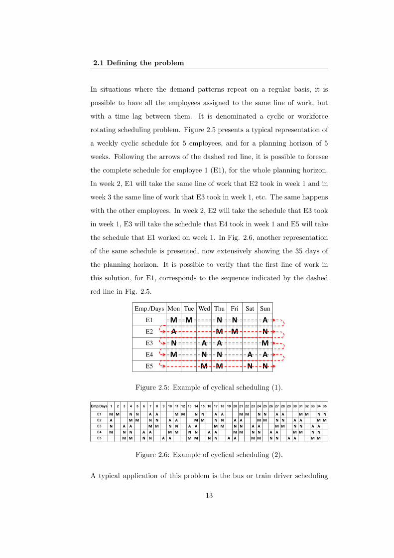
In situations where the demand patterns repeat on a regular basis, it is
possible to have all the employees assigned to the same line of work, but
with a time lag between them. It is denominated a cyclic or workforce
rotating scheduling problem. Figure 2.5 presents a typical representation of
a weekly cyclic schedule for 5 employees, and for a planning horizon of 5
weeks. Following the arrows of the dashed red line, it is possible to foresee
the complete schedule for employee 1 (E1), for the whole planning horizon.
In week 2, E1 will take the same line of work that E2 took in week 1 and in
week 3 the same line of work that E3 took in week 1, etc. The same happens
with the other employees. In week 2, E2 will take the schedule that E3 took
in week 1, E3 will take the schedule that E4 took in week 1 and E5 will take
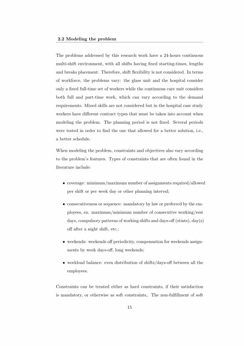
the schedule that E1 worked on week 1. In Fig. 2.6, another representation
of the same schedule is presented, now extensively showing the 35 days of
the planning horizon. It is possible to verify that the first line of work in
this solution, for E1, corresponds to the sequence indicated by the dashed
red line in Fig. 2.5.
Emp./Days Mon Tue Wed Thu Fri Sat Sun
E1 M M N N A E2 A M M N E3 N A A M E4 M N N A A E5 M M N N
Figure 2.5: Example of cyclical scheduling (1).
Emp/Days 1 2 3 4 5 6 7 8 9 10 11 12 13 14 15 16 17 18 19 20 21 22 23 24 25 26 27 28 29 30 31 32 33 34 35
E1 ! ! " " # # ! ! " " # # ! ! " " # # ! ! " "
E2 # ! ! " " # # ! ! " " # # ! ! " " # # ! !
E3 " # # ! ! " " # # ! ! " " # # ! ! " " # #
E4 ! " " # # ! ! " " # # ! ! " " # # ! ! " "
E5 ! ! " " # # ! ! " " # # ! ! " " # # ! !
Figure 2.6: Example of cyclical scheduling (2).
A typical application of this problem is the bus or train driver scheduling
13

Chapter 2. Staff scheduling problems
problem, where timetables usually repeat on a weekly basis. In the oppo-
site situation are call centers, where demand fluctuates every week and so
schedules are typically acyclic. Cyclic scheduling has the advantages of pro-
viding an equal distribution of shifts and days-off among all employees and
of providing stability, since employees know their schedule some time in ad-
vance and can plan their lives according to their future availability. On the
other hand, they lack flexibility, being much less adjustable to last-minute
changes.
2.2 Modeling the problem
Different work environments imply different requirements and, consequently,
staff scheduling problems with distinct features naturally arise. Some of the
main differentiating dimensions that have been explored in the literature
are:
• the adopted planning period, which can range from few days to several
weeks or months up to one year, or can be user-defined;
• the operating hours of the organization, which can work in a 24-hours
continuous or in a less than 24-hours discontinuous operation;
• the workforce, which can be composed of employees with: single or
mixed contract types (full-time/part-time), different skills, distinct
productivity levels, different availability and/or individual personal
preferences; employees substitutability rules, based on hierarchy or on
specific skills for example, may be considered;
• shift flexibility: working shifts can be fixed or can vary in terms of
starting-time, length, placement and/or duration of breaks; overlap
between shifts may be considered.
14
2.2 Modeling the problem
The problems addressed by this research work have a 24-hours continuous
multi-shift environment, with all shifts having fixed starting-times, lengths
and breaks placement. Therefore, shift flexibility is not considered. In terms
of workforce, the problems vary: the glass unit and the hospital consider
only a fixed full-time set of workers while the continuous care unit considers
both full and part-time work, which can vary according to the demand
requirements. Mixed skills are not considered but in the hospital case study
workers have different contract types that must be taken into account when
modeling the problem. The planning period is not fixed. Several periods
were tested in order to find the one that allowed for a better solution, i.e.,
a better schedule.
When modeling the problem, constraints and objectives also vary according
to the problem’s features. Types of constraints that are often found in the
literature include:
• coverage: minimum/maximum number of assignments required/allowed
per shift or per week day or other planning interval;
• consecutiveness or sequence: mandatory by law or preferred by the em-
ployees, ex. maximum/minimum number of consecutive working/rest
days, compulsory patterns of working shifts and days-off (stints), day(s)
off after a night shift, etc.;
• weekends: weekends off periodicity, compensation for weekends assign-
ments by week days-off, long weekends;
• workload balance: even distribution of shifts/days-off between all the
employees.
Constraints can be treated either as hard constraints, if their satisfaction
is mandatory, or otherwise as soft constraints,. The non-fulfillment of soft
15
Chapter 2. Staff scheduling problems
constraints is often penalized, for example in the objective function when
using mathematical programming models or in the evaluation function in a
metaheuristic approach.
The models proposed in this work consider all these types of constraints
as hard constraints. Emphasis is yet given to the formulation of sequence
constraints that, to the best of our knowledge, has not been proposed before
in the literature. The workload balance is a main concern for all the problems
addressed. Weekend-off periodicity constraints were considered in the glass
industry case study and the hospital model was extended in order to account
for planned absences.
Types of objectives that are often used to model the staff scheduling problem
include:
• to minimize total labour costs;
• to maximize the percentage of the contractual work hours assigned or
to minimize the percentage of the unassigned hours;
• to minimize workforce size;
• to minimize the gap between assignments and demand (under or over
coverage);
• to minimize the gap between assignments and employees’ preferences;
• to balance the workload between employees;
• to maximize employees satisfaction.
Although having different objective functions, all the problems studied in
this work share the goal of achieving a balanced and fair schedule for all
workers. In the glass unit problem this is directly formulated in the objective
function. In the continuous care unit problem, the objective function seeks to
16
2.2 Modeling the problem
minimize the part-time requirements. In the hospital problem, the objective
function looks for the minimization of the deviation between assigned and
contracted hours.
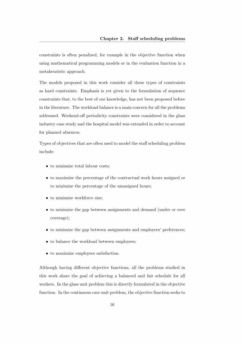
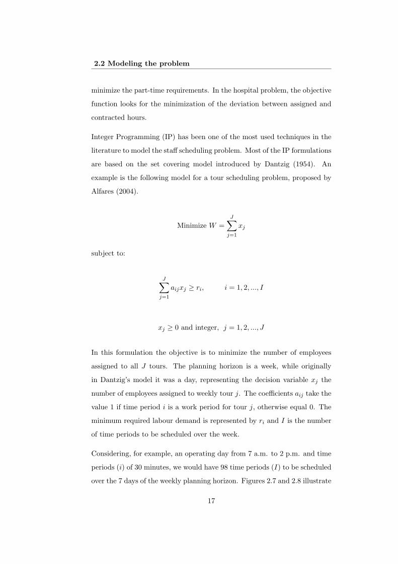
Integer Programming (IP) has been one of the most used techniques in the
literature to model the staff scheduling problem. Most of the IP formulations
are based on the set covering model introduced by Dantzig (1954). An
example is the following model for a tour scheduling problem, proposed by
Alfares (2004).
Minimize W =J∑j=1
xj
subject to:
J∑j=1
aijxj ≥ ri, i = 1, 2, ..., I
xj ≥ 0 and integer, j = 1, 2, ..., J
In this formulation the objective is to minimize the number of employees
assigned to all J tours. The planning horizon is a week, while originally
in Dantzig’s model it was a day, representing the decision variable xj the
number of employees assigned to weekly tour j. The coefficients aij take the
value 1 if time period i is a work period for tour j, otherwise equal 0. The
minimum required labour demand is represented by ri and I is the number
of time periods to be scheduled over the week.
Considering, for example, an operating day from 7 a.m. to 2 p.m. and time
periods (i) of 30 minutes, we would have 98 time periods (I) to be scheduled
over the 7 days of the weekly planning horizon. Figures 2.7 and 2.8 illustrate
17

Chapter 2. Staff scheduling problems
this problem with the correspondent staff needs (ri) for each planning time
period and the matrix of coefficients aij , for J = 1,...,4 tours.
Figure 2.7: Example of a weekly scheduling demand requirement.
Figure 2.8: Example of the weekly scheduling aij matrix data. aij take thevalue 1 if time period i is a work period for tour j, and 0 otherwise.
The model associates to each tour (defined by a shift and break periods
combination) an explicit decision variable xj . In problems with high shift
flexibility, having different shift start, finish or break times, different shift
lengths, etc., this formulation associates a separate integer variable to each
variation of each of these features and therefore, the number of variables
can increase in such a way it is very difficult or even impossible to get an
optimal solution. To overcome this drawback some authors have worked
on the problem formulation in order to reduce the model size using, for
example, implicit modeling. This technique associates each decision variable
to a shift-type or a tour-type. A shift type can be a possible combination of
shift starting time, shift length and break window (interval of time in which
a break can start), for example. Additional constraints are introduced in
order to ensure the correct placement of breaks. A tour-type can have fixed
starting-times for every day of the tour or variable starting-times. In this last
situation, a start-time band can be defined, which is a range in which shift
start-times can vary within a single tour. When start-time bands contain
shifts with the same coverage of periods they are named overlapping start-
18

2.2 Modeling the problem
time bands. Implicit modeling has proven to be particularly important
in those staff scheduling problems that deal with variable shift starting-
times and with breaks placement. For detailed information and practical
applications of this technique along the last decades we refer to Bechtold
and Jacobs (1990), Brusco and Johns (1996), Aykin (2000), Isken (2004),
Addou and Soumis (2007) and Rekik et al. (2010).
In order to overcome the complexity of solving large-size set covering prob-
lems, some authors have explored network flow formulations (Balakrishnan
and Wong (1990), Cezik et al. (2001), Moz and Pato (2004)). In a network
flow model, the source node can correspond, for example, to the begin-
ning of the first day and the sink node to the end of the last day of the
planning period. Each node corresponds, then, to the end of a day and to
the beginning of the following day. Each work shift or rest period is rep-
resented, in the same example, by an arc. Each path from the source to
the sink node represents an alternative feasible pattern of work and rest
periods, which satisfies the sequence and maximum/minimum consecutive
shift/days-off blocks constraints. This option allows for a simple visual rep-
resentation of every feasible tour, which can be significantly advantageous
in problems with many sequence constraints. There are other alternative
representations, though, that have been adopted by different authors.
While coverage requirements are typically formulated as hard constraints,
workload balance and sequence constraints are often treated as soft con-
straints, i.e., constraints that can be violated, though at a defined cost added
to the objective function. Goal programming or multi-objective techniques
are used to incorporate these constraints into the scheduling models. Devia-
tions from desired patterns of shifts, patterns of working and rest days, ratio
between number of night and day shifts or other requirements are penalized
in the objective function, which seeks the minimization of the sum of the
weighted deviations (see, for example, the work of Topaloglu and Ozkara-
19
Chapter 2. Staff scheduling problems
han (2004), Azaiez (2005), Burke et al. (2010b) or Castillo et al. (2009)).
With these formulations the user can analyze the impact of giving different
weights to each of the goals. This sensitivity analysis can be very helpful in
supporting the decision of choosing the most convenient solution from a set
of feasible solutions.
Cote et al. (2009) divide mathematical programming formulations into three
categories: compact assignment, explicit set covering and implicit set cov-
ering formulations. The last two have already been briefly presented in this
section. Compact assignment formulations “use decision variables to assign
activities to each employee at each period” of time. It is our conviction
that the models proposed in this work can be classified as compact assign-
ment formulations as will be explained in detail in Chapters 4 to 8. Our
formulation uses binary variables to assign the working and rest shifts to
each employee in each of the days of the planning period. It cannot be de-
fined as a common assignment problem since, exception made for the glass
unit problem, there is not a one to one assignment relationship. Although
each employee can be assigned to only one shift, either a work or a rest
shift, the same shift can be allocated to more than one employee. Demand
coverage, consecutiveness and sequence restrictions are addressed as hard
constraints. Workload balance is also tackled by hard constraints, imposing
a cyclic scheduling approach to the model.
2.3 Reviewing related works in the literature
2.3.1 Surveys and general works
The developments on staff scheduling problems, their applications, models
and solution methods reported in the literature, have been collected and
reviewed by several authors over the last four decades.
20

2.3 Reviewing related works in the literature
Ernst et al. (2004a) present one of the most comprehensive surveys of the
staff scheduling problem. More than 700 published papers are classified ac-
cording to: the problem type (or sub-problem) addressed, the solution ap-
proach and the application area. In order to classify the sub-problems, Ernst
et al. propose a framework based in several categories, which include, by or-
der of representativeness: crew scheduling, tour scheduling, flexible demand,
workforce planning, crew rostering, shift scheduling, cyclic rostering, days-
off scheduling, shift demand, task based demand, demand modeling, task
assignment, shift assignment, among others. Some of these sub-problems
have already been described in 2.1. For a detailed description of all the
categories see Ernst et al. (2004b).
In a very recent work, Van den Bergh et al. (2012) review 291 articles pub-
lished from 2004 onwards. Papers are categorised according to four main
topics: 1) personnel characteristics (contract type, skills, individual/team)
decision delineation and shifts definition (overlap, start-time, length); 2)
constraints (hard/soft, coverage, time-related, fairness and balance), per-
formance measures (different costs) and flexibility (related to constraints);
3) solution method and uncertainty incorporation (uncertainty of demand,
arrival and capacity) and 4) application area and applicability of research.
A list of the journals with more than 3 publications on personnel scheduling
is also included. All manuscripts are listed and categorised in 16 detailed
tables, allowing for a straightforward usage of the information. Some rele-
vant findings about the reviewed papers can be highlighted. The coverage
constraint is a key constraint, with almost 75% of the authors defining it
as a hard constraint. When considered, the balance constraint is modelled
as a soft constraint by almost all the researchers. The consecutiveness and
sequence constraints are tackled as soft or hard according to the origin of the
imposition, whether if it is a legal setting or a preference scenario, for exam-
ple. In terms of solution methods, mathematical programming approaches
21

Chapter 2. Staff scheduling problems
and metaheuristics lead the choices of the authors. In a innovative perspec-
tive, this survey work also addresses the integration of uncertainty in the
decision-making process as well as the applicability of the staff scheduling
research in the real-world setting.
Transportation systems, nurse scheduling and call-centers are among the
most explored application areas of the staff scheduling problem in the lit-
erature. Within the transportation sector, the airline crew scheduling and
the bus driver scheduling appear as the most studied problems. Surveys
on the airline crew scheduling can be found in Arabeyre et al. (1969), in
Etschmaier and Mathaisel (1985) and more recently in Gopalakrishnan and
Johnson (2005). For an overview of advances in the bus driver scheduling
problem see Wren and Rousseau (1995) and Wren (1998). Reference review
studies in nurse scheduling are the works of Warner (1976), Silvestro and
Silvestro (2001) and Burke et al. (2004). A tutorial and state-of-the art on
telephone call centers is presented in Gans et al. (2003).
In a tour scheduling scope survey, Alfares (2004) reviews over 70 papers pub-
lished between 1990 and 2001, comparing mathematical models and classify-
ing the studies, according to the solution methods adopted, in ten categories:
manual solution, IP, implicit modeling, decomposition, goal programming,
working set generation, LP-based solution, construction/improvement, meta-
heuristics and other methods (network-flow models, expert systems, heuris-
tics, etc.). During the period considered in the survey, metaheuristics (mainly
simulated annealing) were the most used techniques, followed by construc-
tive/improvement methods, decomposition, manual solution and IP. How-
ever, when considering only the second half of the survey period, the trend
seems to be more favorable to the use of metaheuristics, IP and manual
solutions rather than to the other methods. In an era of technology ad-
vances, it is quite surprisingly that manual solutions appear as one of the
most popular methods, but the truth is that staff scheduling is still done
22
2.3 Reviewing related works in the literature
manually in some activity sectors, like hospital wards, for example. Laporte
(1999) suggested the manual design of cyclical schedules, arguing that IP
formulations are too rigid to be applicable to real-world problems.
In an earlier work, Baker (1976) reviews mathematical programming formu-
lations for the shift and the days-off scheduling problems with cyclic demand
patterns. Baker highlights the importance of demand modeling as a crucial
stage within the shift and the days-off problems. Although they were typ-
ically treated separately, Baker suggests the development of an integrated
model for both problems, since they share a common context and a depen-
dency in terms of staff requirements. In the same work, Baker discusses
the trend of the researchers to simplify real problems, treating demand in
a deterministic way, even when the problem has probabilistic features. Ap-
plication areas of staff scheduling problems tackled in this survey include
mainly service activities as baggage handlers, bus drivers, telephone opera-
tors or toll collectors.
Considering the complexity of the staff scheduling problem and its variants,
it is easy to foresee the difficulty in finding a homogeneous problem clas-
sification approach among the several surveys published in the literature.
Every author proposes its own definitions scheme, which makes it harder
for the comparison of problems and the evaluation of achieved results. In
a recent work, De Causmaecker and Vanden Berghe (2011) overcome this
gap, proposing a framework for the classification of staff scheduling prob-
lems in services. It considers three categories: personnel environment, which
includes different types of personnel constraints and skills; work character-
istics, which refers to coverage constraints and shift types; and optimisation
objectives. Such a classification system allows the benchmarking of prob-
lems, the evaluation of the instances in terms of hardness and complexity
and also the comparison of solution approaches.
23
Chapter 2. Staff scheduling problems
In a conceptual work, Warner (1976) identifies an interesting set of indicators
to measure schedules’ performance in terms of: coverage, quality, stability,
flexibility, fairness and cost. Coverage measures how close the solution fits
the demand requirements. The quality of a roster indicates how well the
schedule matches the employee’s request or wish, while fairness is a measure
of how the employee feels about his/her schedule when compared to the
schedules of the other employees. Stability is related to predictability and
cost is a measure of resource consumption in developing the schedule.
2.3.2 Specific works
Several variants of the staff scheduling problem can be found in the lit-
erature, concerning the different model features that were created due to
practical needs of the problems, the modeling options and the solving meth-
ods. Our specific literature review focuses on those variants that share
common features with our problems (mixed contract types, sequence and
consecutiveness constraints, workload balance, variable demand) and that
is, somehow, work of acknowledged relevancy. In order to give the reader
an overview of the published related work, some additional references are
also included. It is not intended to make an exhaustive literature review,
though. In the present sub-section, studies are organized according to two
approaches: non-cyclical and cyclical. The latter is the one adopted in our
case studies. The main features and the adopted solution methods are de-
scribed for each case. The most common modeling techniques have already
been overviewed in Section 2.2 and some related studies were then pointed
out.
Examples of non-cyclical optimization approaches to solve problems consid-
ering a mixed workforce are the works of Bard et al. (2003), Eitzen et al.
(2004) or Rong (2010). All of them use IP techniques.
24

2.3 Reviewing related works in the literature
Bard et al. (2003) address the tour scheduling problem of a postal service
company, which includes full and part-time staff as well as variable shift
starting-times. Bard et al. decompose the scheduling problem in smaller
problems, which are easier to solve. In a first phase, staff levels and shifts
are determined by an IP model, where the objective is to minimize the
weekly total cost of the workforce. While the weekly cost of a shift for
full-time staff is fixed, the weekly cost of a part-time shift varies since it
can have several different lengths. In a following post-processing phase, the
days-off problem and the assignment of breaks in each shift are addressed
in parallel. A constructive algorithm is used to solve the days-off problem,
while the placement of breaks is tackled with a network flow formulation
and solved by the CPLEX solver with OPL Studio. A final VBA procedure
is called to build the weekly schedule for each employee.
Eitzen et al. (2004) develop a set of three IP based methodologies (column
generation, column subset and branch-and-price) for solving a multi-skilled,
non-hierarchical workforce scheduling problem of a power station unit. The
workforce contains a fixed set of 48 full-time and 8 part-time employees,
which are grouped according to their skills. The unit works in a three fixed
8-hour shift scheme (day, afternoon and night) and with a demand forecasted
for a 12 weeks period. Schedules are built for 2 week-cycles. Emphasis
is given to ensuring equity between schedules of the employees with the
same skills, which is achieved by means of a score levels assignment. Each
employee is given a different score for a day, night or weekend shifts. The
cumulative score of the past schedules for an employee is used to assign
to him/her the most convenient shifts in the current planning period. The
equity for an employee is the cumulative score over the planning horizon and
it is different from group to group. The three solution methodologies are
compared for a set of instances, varying the size of the workforce, the number
of skills and the demand levels. The problems are solved with CPLEX. All
25

Chapter 2. Staff scheduling problems
the three methods revealed limitations when looking for an optimal solution
given the large dimension of the problems. Eitzen et al. (2004) use the fact
of having to deal with a multi-skilled workforce and a fluctuating demand to
justify the use of an acyclic approach rather than a cyclic one. We believe
we can refute this theory with the hospital case study, described in Chapter
7.
Staff mixed skills and weekend off requirements are explored in the work
of Rong (2010). Two IP formulations are developed that simultaneously
determine workforce size with different employee types (skills) and assign
workers to jobs satisfying a fluctuating demand across the hours of the day
and across the days of the month. The objective is to minimize the total
workforce cost. The models differ in the way that lunch breaks assignment
is addressed: a general IP formulation assigns lunch break hours according
to worker types and a binary IP formulation that assigns lunch break hours
explicitly to individual workers. Although it leads to a problem with a
larger size, the second approach has a simpler model structure. Models
were solved with CPLEX and results show that the binary approach is more
efficient than the general one. A novel framework is proposed by Rong that
introduces a 0-1 matrix for the worker type-skill representation. This matrix
accommodates both hierarchical and non-hierarchical workforce scheduling.
Hierarchical rules have also been the scope of the work of Ulusam Seckiner
et al. (2007).
Beaulieu et al. (2000) propose a goal programming approach to solve the
scheduling problem of physicians in a hospital emergency room in Mon-
treal. The proposed model uses binary assignment decision variables, but
also considers succession and deviation variables. Succession variables are
used to formulate the constraints related to the sequences of working shifts
and days-off. For each sequence rule imposed to the model a different type
of succession variables is defined and several constraints are added. This
26

2.3 Reviewing related works in the literature
formulation is useful to address this particular problem but it may not be of
easy generalization and adaptation to different shift sequence requirements,
namely in different application areas. Deviation variables represent devia-
tions from the goals defined for the constraints that ensure the fairness or
balance of the schedule, such as the number of working hours a physician
must work per week or the distribution of some night and evening shifts
among the physicians. The objective function seeks the minimization of a
weighted sum of the goals. Beaulieu et al. tried to solve the model us-
ing branch-and-bound techniques but that has proven to be impracticable
given the large size of the problem. Some constraints had to be relaxed or
eliminated from the model in order to get a feasible solution, although of
poor quality. An iterative procedure was then adopted to improve this first
solution: firstly, the violated rules are identified and the corresponding con-
straints are added to the model; secondly, branch-and-bound is used to find
a new schedule, better than the initial solution. A good quality schedule was
generated in less time than the time needed by the real (human) planner of
the hospital.
When an optimal solution is not mandatory, heuristics and metaheuristics,
such as tabu search (Burke et al. (1999, 2001)) and genetic algorithms (Aick-
elin and White (2004)), as well as constraint programming (Abdennadher
and Schlenker (1999)) are alternative approaches that have been widely used
to address consecutiveness and workload balance constraints.
Brusco and Johns (1996) propose a general set covering formulation to model
the discontinuous tour scheduling problem considering both part-time and
full-time employees with variable levels of cost and productivity. To solve
the problem, a mixed IP heuristic is presented. In a more recent work,
Thompson and Goodale (2006) also address the problem of employees with
different productivity levels but use a nonlinear representation of the prob-
lem, incorporating the stochastic nature of the demand in service operations
27

Chapter 2. Staff scheduling problems
(customer arrivals). Thompson and Goodale use simulated annealing based
heuristics to solve their problem.
Brucker et al. (2008) propose a decomposition approach based on a two-stage
adaptive construction procedure to solve the nurse scheduling problem in a
fixed 4-shift environment. Three types of constraints are defined: sequence,
schedule and roster related. Sequence constraints define the sequences of
shifts for each nurse, according to his/her skills. Schedule constraints are
associated with all the rules that limit the construction of the schedule.
Roster constraints are essentially coverage constraints. The first stage of
the proposed procedure consists in constructing shift sequences for nurses
by only considering the sequence constraints. In a second stage, the schedule
for one nurse as well as the roster for all nurses are iteratively built, based
on the sequences obtained in the previous phase and considering now the
schedule and roster rules. The novelty of the developed procedure is to sep-
arately account for the problem’s constraints, considering first the sequence
and schedule and roster constraints after. Although the first stage calls for
an exhaustive enumeration of all shift sequences, the achieved results are
promising and the method has proven to be efficient.
A randomized greedy procedure is proposed in Carrasco (2010) to balance
the workload in a long-term (annual) planning horizon. This work is one of
the few exceptions that tackle the balance constraints as hard. Employees’
preferences are not considered in that case, which decreases the complexity
of the problem.
A novel heuristic approach combining mathematical programming with local
search procedures is proposed in the recent work of Constantino et al. (2011),
where the objective is to balance employees’ satisfaction levels, measured in
terms of assigned versus preferred working shifts in a specific day. The
combination or hybridization of different techniques is becoming popular,
28

2.3 Reviewing related works in the literature
since it can explore the features of all the used methods. Examples of hybrid
approaches are described in Qu and He (2009), Valouxis and Housos (2000)
or Sellmann et al. (2000).
Hyperheuristics are a more recent technique that uses a high-level strategy
to manage a set of low-level heuristics (or parts of heuristics). Instead of
evaluating a space of solutions for a given problem, this method evaluates
a set of heuristics, at each stage of the solution construction process. A
deep insight on this topic can be found in Burke et al. (2010a). Examples
of the application of hyperheuristics to nurse scheduling and to a home care
scheduling problem are reported in Burke (2003) and Misir et al. (2010),
respectively.
Many of the works mentioned so far tackle the problem of determining the
optimal workforce size before or simultaneously with the shift scheduling or
the days-off scheduling. And they are all acyclic scheduling problems. In
fact, as far as we could perceive, problems with variable workforce size have
been widely studied in the literature of acyclic staff scheduling. However,
that is not the case of the problems we address in this work, which are
tackled with a cyclic approach. All of them have a fixed set of full-time
employees and the continuous care unit has an additional set of part-time
employees, which are requested according to the demand requirements.
In problems of non-cyclic nature, cyclical approaches are avoided because
of their apparent inflexibility to deal with unexpected changes in schedules
(absences, etc.), but they guarantee the balance and fairness of the schedule,
in terms of workload distribution and days-off, and they are predictable.
Cyclic scheduling problems have been studied by some authors. Exhaustive
enumeration of all feasible patterns (or sequences) of working shifts/days and
days-off is often a common method in the construction of cyclical schedules
to overcome sequence restrictions, which are typically a factor of complexity
29

Chapter 2. Staff scheduling problems
to most of the models. Making use of his wide practical experience, Laporte
(1999) argues that cyclical scheduling is more of “an art than a science”,
suggesting that in order to get workable solutions, some of the problem’s
rules must be violated.
Chan et al. (2001) propose a constraint programming approach to solve a
cyclic scheduling problem considering an annual planning horizon. In ad-
dition to common work rules and legal constraints, annual leaves are also
included in this case. Work cycles are not just repeated along the planning
horizon, but rather relaxed (extended or shortened) to allow for days-off.
The constraints developed in this approach were embedded in a more com-
plete software application that has been successfully implemented in real
work context, producing annual schedules for 150 employees. Another con-
straint programming algorithm is proposed by Laporte and Pesant (2004).
Beaumont (1997) uses a multi-objective mixed integer formulation to model
the days-off scheduling problem in a long-term planning horizon (47 and 48
weeks cycle). Constraints are imposed on consecutive working and off days
and on the weekly mean workload. The objective function is a weighted
sum of three components: the preference of employees for long work periods
and long breaks, the balance of the workload among employees in a 30-
day period and the management decision of having a number of employees
on duty on each day of the week proportional to the demand on that day.
The decision variables defined are binary variables that indicate whether
a specific day is a workday or a day-off. This is a simpler problem than
the ones considered in our work, since the assignment of shifts to working
days and to each employee is not considered. The model was solved with a
CPLEX solver. Three schedules were generated for each cycle, considering
different goal weights, to be analyzed by the client.
Alfares (1998) addresses the days-off scheduling problem with five working
30
2.3 Reviewing related works in the literature
days and two days-off cycles. The problem is decomposed in two stages.
In a first phase, an expression to calculate the minimum workforce size
is determined. In a later phase, that value is included as a constraint in
the linear programming model of the problem, which is a relaxation of the
IP model, ensuring an optimal integer solution. This approach has the
advantage of being applicable to problems with different days-off pattern
costs.
A decomposition two-phase framework is also developed by Balakrishnan
and Wong (1990), who propose a network flow formulation to solve a cyclic
scheduling problem with fixed shifts. The optimal solution is found using a
shortest path based technique. A novel approach is presented by Hao and Lai
(2004), who solve a cyclic scheduling problem for airport ground staff with
a neural network methodology. Experiments revealed encouraging results
when compared with the solutions obtained by simulated annealing, tabu
search and genetic algorithms.
Heuristics and metaheuristics based methods have also been used to solve
the cyclic scheduling problem, as for example in the work of Mora and Mus-
liu (2004) and Musliu (2006). Mora and Musliu (2004) propose a generic
algorithm based methodology while Musliu (2006) explores the tabu-search
potentialities to develop and compare a set of heuristic procedures to au-
tomatically generate cyclic schedules. In the last mentioned work, Mus-
liu uses a benchmark data set to compare results, which is available in
http://www.dbai.tuwien.ac.at/staff/musliu/benchmarks. These examples
are used to analyze the performance of our formulation, as will be described
in detail in Chapter 8.
31

Chapter 2. Staff scheduling problems
2.4 Summary
This chapter introduced the staff scheduling problem: main concepts, fea-
tures and applications. The aim was not only to provide background on the
topic, but also to situate the problems addressed by this research work. An
overview of modeling aspects was presented, with emphasis on IP techniques.
The related literature was reviewed, focusing on those works that shared
features with the problems studied in our work. This analysis revealed an
existing trend to develop IP models for specific applications and justified the
opportunity to build a general model that could be easily adapted to solve
different problems. This model should be flexible to accommodate complex
but relevant constraints, such as employee preferences and the equity of the
staff schedules. The main challenge was to formulate such a general model
using IP techniques and apply it to different real-life problems, solving them
to optimality.
32

Chapter 3
Hospitality management
This chapter is dedicated to the description of hospitality management as a
potential application area of staff scheduling problems. The first section in-
troduces the concept of hospitality and gives an overview on how hospitality
management is discussed in the research literature. A reference to the con-
textualization of hospitality activities in the Portuguese setting is included.
Afterwards, some insights on the staff scheduling problem applied to hospi-
tality management operations are presented. Firstly, its main features are
pointed out and an attempt to approximate it to applications in other areas
that have been already extensively studied in the literature is made. This
exercise is followed by a literature review of the related works. To close the
chapter, a final outlook on the results of the research work described in this
chapter is given.
3.1 Hospitality management
Hospitality is not a recent activity. In the social sense of the concept it
dates from ancient times, where many societies had traditions of travelers
protection and welcoming. King (1995) overviews historical and sociological
roots of hospitality and proposes a model emphasizing the importance of
33
Chapter 3. Hospitality management
relationships between individuals (hosts, guests/ customers, employees) in
any hospitality context, whether it takes place in a private or in a commercial
setting.
Hospitality and hospitality management have been the scope of many re-
search articles, essentially in the social sciences field, where the discussion
has been focused on defining a common, generically accepted, definition
and on the development of a framework to be the basis of an independent
academic discipline.
Although still being often merged with tourism and leisure sector activi-
ties, hospitality services are a growing activity sector in a society where
customer’s satisfaction and well-being run the market. They usually in-
clude hotels, restaurants and other sort of lodging, food and drinks services
providers. Due to the specifications of the kind of service provided, hos-
pitality management has to deal with complex variables and constraints.
An unpredictable customer demand, a multiskilled workforce, different staff
labour contracts’ demands, employees satisfaction and costs minimization
are just some of the conditioning issues that an organization has to deal
with in order to achieve a flexible, profitable and high quality service provi-
sion.
A survey undertaken by Enz (2009), in cooperation with the Center for
Hospitality Research of Cornell University, identified human resources man-
agement as the subject of most concern for hotel managers, above other
aspects such as economic or environmental problems, and regardless of the
geographical location. The study was based on the statement of 243 expe-
rienced hotel executives from six countries. This highlights the importance
and worldwide relevance of human resource management to a hospitality or-
ganization. Staff scheduling are typical problems to solve within this area.
There is however a big lack of published articles focusing on these problems
34

3.1 Hospitality management
applied to the hospitality sector, as realized by Ernst et al. (2004a), in op-
position to other application areas such as hospitals, transportation or call
centers.
One of the reasons for the lack of research articles focusing on staff scheduling
problems in hospitality is perhaps the lack of a consensual and generically
accepted definition of the activity itself. Etymologically, the word hospital-
ity, in Latin hospitalities, has its origin in hospes or hospitis (genitive), which
means foreigner or guest. Dictionary definitions include “cordial and gener-
ous reception of or disposition toward guests” (“hospitality”, The American
Heritage Dictionary of the English Language) and “kindness in welcoming
strangers or guests” (“hospitality”, Collins Essential English Dictionary).
It is synonym of hospitableness and widely used to define welcoming host-
guest relationships, being thus traditionally associated with cultural and
social values of each community.
In the industrial context, the term hospitality has been adopted mainly in
the English-speaking countries to refer to the activity of hotels, restaurants
and other sort of lodging, food and drinks services’ providers, whether it
takes place in a public/ commercial or in a private/ social context. Lashley
(2008) argues that this framework can be understood as an effort to “create
a more favorable impression” of these activities, promoting a further hos-
pitable commercial activity and letting the profit provision motivation re-
main in the background. While British researchers have traditionally based
the discussion on this definition, American academics tend to use a broader
meaning of hospitality, associating these activities with others under the
tourism field, such as travel, leisure or entertainment.
In a first essay, hospitality management would then be intuitively defined as
the management of those hospitality activities. In accordance, Brotherton
and Wood (2008) write that hospitality management is a generically used ex-
35
Chapter 3. Hospitality management
pression to easily replace other labels such as “hotel management”, “restau-
rant management” or “catering management”, but consequently none or few
reflection has been given to the genuine meaning or nature of hospitality.
They state that hospitality research has been characterized throughout the
years by an unsystematic and scattered analysis, rendering a meaningful
synthesis very hard to achieve.
In the academic community, researchers have been seeking out the devel-
opment of the specialist discipline of hospitality management that would
embody a theoretical framework and link it to the industry sector, but the
lack of a consensual definition of hospitality has effectively been a barrier
both to research progress (Jones (1996), Taylor and Edgar (1996)) and to
the creation of a robust and mature branch of knowledge. The discussion
has been driven by some authors into the field of cultural and social sciences
(Brotherton (1999), Hemmington (2007), Jones (2004), Lashley (2008)), in-
corporating in the debate the importance of studying hospitality from a
wider perspective rather than the commercial one. The contribution of
authors from different fields of research and their vision’s diversity could
potentially be a major value but it could also be understood as a reflex of a
fragmented and unstructured hospitality research.
King (1995) introduces a hospitality model based on the interaction of so-
cial “rituals” in the commercial operation, associated with the process of the
guest arrival, welcoming and departure. The author defines hospitality as
a host-guest relationship between individuals, taking place in a commercial
or private setting, whose success is assessed by the clear perception of the
guest needs and their genuine satisfaction by the host. This perspective un-
derlies an unconditional moral duty of hospitable behavior that can, at the
edge, merge the meanings of hospitality and hospitableness, which Brother-
ton (1999) contests, arguing that hospitableness has a much broader scope
than hospitality activities. In fact, hospitable concerns are a competitive
36
3.1 Hospitality management
advantage in any activity where there is a “service” relationship with the
customers, whether it is from the hospitality sector or not.
Believing that hospitality is a time evolving phenomenon, i.e, that hospital-
ity’ characteristics change over time, Brotherton (2006) presents a concep-
tual model for hospitality comprising four dimensions: spatial, behavioral,
temporal and physical. These dimensions help to analyze the extent of
hospitality in terms of place of occurrence, motivational aspects, time and
material features involved. In this conceptual model, the nature, incidence
and forms of hospitality in a particular society in any given time period,
expressed by domestic or commercial hospitality behavior, are a function of
the human and natural resources available, which in turn are conditioned
by the economic, socio-cultural, politico-legal and technological conjuncture.
The author tried to operationalize this model through case studies (Broth-
erton and Wood (2008)) in two hotels and later in two fast food restaurants,
where guests/customers where asked to participate through an interview,
associating words that best fitted their notion of hospitality. Although this
exercise did not produce statistically significant results in terms of the in-
fluence of social factors (like age, gender, occupancy, etc.), it did provide
inputs for understanding guests’ perception of the meaning of hospitality
that still needs to be further explored.
The comprehensive approach of studying the commercial hospitality activity
from a wider social sciences perspective has indeed been quite controversial,
as it turned out to happen after the publication of the book “In search of
hospitality: theoretical perspectives and debates” by Lashley and Morrison
(2000). The referred work presents the nature of hospitality from several
views, from Anthropology to Marketing, and proposes an integrated “three-
domains approach”: the private, the social and the commercial domains.
The main idea of this conceptualization is to consider and evaluate the
effect of the social and cultural dimensions of hospitality in the commercial
37
Chapter 3. Hospitality management
or business activity, despite their blurred boundaries. The book also defends
the existence of hospitality management as an independent activity, apart
from any other management activity.
Slattery (2002) is one of the researchers who is most critical of this approach,
arguing that it overestimates the social side in relation to the economic one
and “excludes the hospitality industry context”. His classification model of
hospitality industry is based on the place where activities effectively take
place: Free-Standing Hospitality Business (hotels, restaurants, bars), Hos-
pitality in Leisure Venues (casinos, cinemas, health clubs), Hospitality in
Travel Venues (airports, bus stations, trains, ferries) and Subsidiary Hospi-
tality (workplaces, health care, education). He thus considers that confining
hospitality to lodging, food and drinks activities falls short since hospitality
necessarily undertakes the management of several other sort of associated
leisure activities, in order to respond to the increasing complexity of cus-
tomer demand.
In his review, Jones (2004) identifies five main hospitality schools of thought:
science model, management, studies, relationship and systems, attesting
that the state of hospitality research is not yet consolidated and there is
a lack of consensus concerning its definition. Even though this diversity
of thoughts persists, the management perspective was recognized to be in a
dominant position in relation to other emerging views. But even from a man-
agement point of view the author finds three different approaches, with their
main divergence in the focus of the research. While the traditional point
of view considers hospitality to be a sub-discipline inside the main man-
agement disciplines, a different conviction uses hospitality as an application
of the main discipline and a third perspective assumes a “multidisciplinary
approach” studying hospitality from several different main management sub-
jects.
38

3.1 Hospitality management
In a recent article, Ottenbacher et al. (2009) analyze the pedagogical and re-
search implications of defining the hospitality discipline. Based on a services
marketing perspective, the authors defend a taxonomical classification, con-
sidering hospitality as a field supported by the economic output of a group of
six related industries: lodging, food services, leisure, travel, attractions and
conventions. Each of these independent industries takes, in turn, “input
from hospitality either directly or indirectly for its survival and success.”
The article suggests the need of exploring separately each one of these ac-
tivities, which are often ignored in the literature, recognizing the diversity
of their constitutive market segments.
In the Portuguese context a translation for the concepts of hospitality or
hospitality management is still missing and consequently there is not a con-
solidated research activity focused in this thematic area, or at least with
an acknowledged published work. A few exceptions include for instance
the work on hotel management efficiency using Data Envelopment Analy-
sis (Barros and Mascarenhas (2005), Barros et al. (2008)). A hospitality
association was created - Hospitality Management Institute (HMI (2008)),
as a result of the cooperation between Turismo de Portugal, ISCTE (In-
stituto Superior de Ciencias do Trabalho e da Empresa), Universidade do
Algarve and ESHTE (Escola Superior de Hotelaria e Turismo do Estoril),
sponsored by the Portuguese Government and the National Strategic Coun-
cil for Education and Training in Tourism, that aims to promote advanced
management training and to support applied research in tourism.
Portuguese hotel and restaurant industries have traditionally been consid-
ered as a part of the tourism sector, for statistics, economic indicators and
sectorial strategies, as well as several other service providers connected to
touristic services, such as travel agencies, touristic operators or leisure ac-
tivities promotors. There are many different associations: Portuguese Ho-
39

Chapter 3. Hospitality management
tel Association (AHP), Association of Hotels and Tourism Enterprises of
the Algarve (AHETA), Association of Restaurants and Associated Indus-
tries of Portugal (ARESP), Portuguese Association of Congress Companies
(APECATE), Portuguese Association of Travel Agencies (APAVT), among
others.
In Portugal there are promising perspectives to the hospitality activities as
the tourism sector is strategically regarded as a priority for the Portuguese
economy, due to its ability to create jobs and wealth and due to its rec-
ognized international competitive advantage. Stakeholders are committed
to the development of the sector, and so is the Government, as is clearly
assumed in the National Strategic Plan for Tourism, where the ambitious
objectives defined aim to reach, by 2015, 20 million tourists and e15 billion
of revenues, what will represent in terms of economic impact over 15% of
GDP and 15% of national employment (Ministry for Economy and Innova-
tion (2011)).
3.2 Staff scheduling in hospitality management
The staff scheduling problem in hospitality services shares common features
with other service activities. It is quite noticeable, for instance, its similarity
with the nurse rostering problem, so deeply explored in the literature. Con-
sidering hospitality in its narrowest sense, as defined in the previous section
of this chapter, which includes mainly lodging units and restaurants, both
problems seek to assign a set of employees to a set of working days, shifts
and rest periods in order to satisfy demand levels, taking into account work
rules, employees’ skills, availability and preferences. The staff scheduling
problem both in hotels and hospitals is typically characterized by an around
40
3.2 Staff scheduling in hospitality management
the clock operation, 7 days per week and a fluctuating demand. The use of
different contract types (e.g. part-time) is therefore a common and necessary
practice.
Of course the place where it takes place and the set of conditions under
which it can be found make the approaches to the rostering problem to be
different in a hospital or in a hotel. The nurse rostering problem takes place
in a hospital unit - a ward, where usually the different skill categories of the
nurse function (e.g. head nurse, regular nurse, caretaker) need to be taken
into account. The considered shift types are usually the conventional 7 or
8 hour shifts: early, late and night. Demand is usually determined with
basis on desired service levels (e.g. nurse/patient ratios) or/and forecasting
techniques and staff levels are defined for each shift and skill category. Work-
load distribution follows a daily pattern, usually ignoring weekends. Work
rules are strict in terms of shift sequence, maximum/minimum number of
consecutive assignments for each shift, periodicity of rest days, etc.
In addition to its lodging core operation, which involves several different
functions (receptionist, concierge, doorkeeper, cleaning staff, maintenance
operator, administrative staff) a hotel usually includes other activities such
as restaurant, bar, leisure spaces, etc. The staff scheduling problem in a ho-
tel may also be applied to a single functional area, for example the scheduling
of the reception staff or the cleaning staff. There are situations, however,
where staff is multifunctional and so an integrated approach is more ap-
propriate, increasing the complexity of the problem to solve. It requires a
high flexibility in terms of shift length, starting and finish times and needs
to manage a bigger diversity of employee contract types as well as multiple
functions. In what concerns work rules, just like in the case of hospitals,
hotels and restaurants are very conditioned by sectorial union agreements
or contracts, namely in terms of working and rest periods. In the current
globalization context, multinational hospitality organizations, and specially
41

Chapter 3. Hospitality management
hotels, must follow the motto: “think globally, act locally”, meaning that
although having general rules, common to all their units, each unit must
have its organization and practice adapted to the local context where they
are placed in. Different cultures and different habits usually mean different
needs. In the hotels case, the majority of the reclaimed service levels are
strategically imposed by its category (number of stars). Staffing needs must
be determined based on the historic data, on guest arrival forecasts, on a
slack for daily late arrivals but also based on the desired service levels.
In a similar way to the case of nurse rostering, important schedule’s char-
acteristics to take into account in hotels are: coverage, quality, stability,
flexibility, fairness and cost (Warner (1976)). These concepts have already
been described in detail in section 2.3. In particular, quality, fairness, stabil-
ity and flexibility are those characteristics that are connected to employees’
preferences and are, therefore, very important to guarantee a motivated and
productive workforce. This is a critical issue in any customer oriented activ-
ity, and specially in services where there is such a deep interaction between
employee/host and customer/guest, as is the case of hospitality operations.
The perception of customer needs and their satisfaction is very dependent
on the performance of every employee. Therefore, employees’ welfare must
be safeguarded. One adoptable approach to the rostering problem in hos-
pitality organizations, and in hotels in particular, is the tour scheduling
problem.
Applications of staff scheduling problems have been explored in many ac-
tivity sectors in the literature, with emphasis on hospitals and transporta-
tion systems (Ernst et al. (2004a)). Hospitality, in turn, has had much
less attention of researchers working in the quantitative field, with very few
published articles, referring mainly to restaurants (Glover (1986), Love and
Hoey (1990), Loucks and Jacobs (1991), Thompson (1996), Eveborn and
Ronnqvist (2004) and Choi et al. (2009)).
42

3.2 Staff scheduling in hospitality management
In an attempt to justify the relevance of staff scheduling for hospitality man-
agers, Thompson proposes a four-stage method for the hospitality industry,
which he presents in a series of four articles: forecasting demand (Thomp-
son (1998a)), translating those forecasts into staff requirements (Thompson
(1998b)), scheduling staff (Thompson (1999a)) and monitoring the schedule
in real-time (Thompson (1999b)).
In the third paper, Thompson (1999a) proposes a methodology for develop-
ing work schedules in hospitality organizations that seeks to balance both
the organization’s and the employee’s goals. A comparison of two traditional
approaches to staff scheduling, one by Dantzig (1954) and the other by Keith
(1979), is presented and their limitations are pointed out. Two new meth-
ods are proposed, under two different perspectives: economic and service
standards, with the objective of achieving the highest schedule’s economic
outcome and optimal service standards respectively. The main difference
between these methods and the classic ones is that employee requirements
are no longer independently set for each planning period but are now instead
taken into account both in the determination of demand levels and on the
actual scheduling process. Assuming that a surplus employee cannot have
the same cost or bring the same benefit/value no matter in which period
he is added, it is possible to maximize the level of service provided or to
develop the best schedule from an economic point of view, as defined by the
organization. An emphasis is given therefore to the importance of satisfying
employees’ preferences, not disregarding their availability and skills and to
the advantage of considering this information in the shifts development pro-
cess. Thompson defends the use of a heuristic procedure in order to reach
a good schedule in a reasonable amount of time in opposition to trying to
find optimal solutions, which is typically too time consuming. The recom-
mended planning horizon is one or two weeks, mainly due to the typical
difficulties in predicting service demand more than two weeks in advance.
43

Chapter 3. Hospitality management
Although presenting it as the outcome of a long work experience, Thompson
does not apply this work to a practical case study. It would be interesting
and certainly of great value to see the application of this approach in a hotel
unit.
Choi et al. (2009) applied Thompson’s framework to a restaurant, where the
workforce is composed of 30 full-time and 19 part-time employees. Staffing
and scheduling problems are both addressed in a weekly planning horizon.
Based on past experience, the management defined a ratio of full-time vs
part-time workers of 6:4, which they assumed to ensure the desired service
levels. The developed IP model assumes that full-time workers have higher
productivity levels than part-timers, but also imply higher costs. The ob-
jective of the problem is therefore to minimize the overall labor costs while
ensuring the appropriate service levels. Results demonstrated an increase in
the overall efficiency of the scheduling system, achieving a reduction in the
labor costs of overstaffing and also in the opportunity costs of understaffing.
This work emphasizes the problem of the high turnover costs associated
with hospitality organizations. An efficient scheduling can contribute to the
engagement of the employees and motivate an increase in the workforce re-
tention rate. The model had some simplifications though, not considering
for example employees’ preferences or availability, which can also be very
relevant to the retention in a job.
Over and understaffing are also addressed in Eveborn and Ronnqvist (2004).
A scheduling software system is developed - SCHEDULER, which is com-
posed by several optimization modules. The main model of the system is
an IP set partioning formulation which is solved using a branch and price
approach. The problem’s features considered include legal constraints and
employee’s preferences. The system provides an interface where the user
can select different weightings between costs and preferences. The fairness
of the schedules is measured through a constraint that limits the sum of
44
3.3 Final reflections
penalty points associated with each schedule. Although the authors men-
tioned that hotels and restaurants are among the organizations where the
SCHEDULER was implemented, those cases are not reported in the study.
Staff scheduling problems in fast-food restaurants have typical features: the
workforce is composed of a set of full and part-time workers, with different
skills and availability. The assignment of employees to tasks or shifts must
cover the requirements of a demand that fluctuates through the hours of the
day. The objective considered is usually to minimize over and understaffing
costs. Glover (1986), Love and Hoey (1990) and Loucks and Jacobs (1991)
solve this problem using three different approaches, respectively: a tabu-
search based procedure, a network flow technique and a goal-programming
formulation solved with a constructive heuristic.
3.3 Final reflections
Although hospitality and hospitality management are subjects that have
been quite explored by social science researchers, they are not commonly re-
ferred in the operations research literature, or more precisely in the schedul-
ing operations literature. But the truth is that there is a point in exploring
rostering and scheduling problems in this area. First of all, because as in
any other activity in the services industry, the importance of staff expen-
diture is typically very significant in the total operating costs. Secondly,
because the quality and efficiency of the service provided by a hotel or a
restaurant have direct impact on its customers’ satisfaction, as in few other
service activities. The social dimension of hospitality, which has been in the
hospitality research agenda in the last decades, increases the complexity of
staff rostering problems in this activity area. It is no longer only a matter
of assuring the required employees’ technical skills, but also of guaranteeing
that they have the right personal competences to interact with customers,
45

Chapter 3. Hospitality management
to understand and satisfy their needs. The staff must be motivated and
engaged. Staff scheduling systems shall therefore account for the workforce
well-fare, considering employees’ preferences in terms of work and rest days,
weekends off and holidays, shifts assignment, shifts change, shifts starting
and finishing times flexibility, compatibility or incompatibility with other
staff elements, etc. Possible approaches to the staff scheduling and rostering
problem in hospitality management, or its sub-problems, may be inspired
by the work that has been comprehensively done both in tour scheduling
and nurse rostering. As exposed before in this chapter, nurse rostering and
hospitality are two activity areas with many similarities concerning rostering
issues. Examples of the few divergences between them include the seasonal-
ity, the weekly and daily cycles operation inherent to hospitality activities,
that contrast with the Winter/Summer seasonal workload distribution of
hospitals. Thompson (1999a) gives a very important contribution to staff
scheduling and rostering in hospitality management. It should have trig-
gered the interest of researchers in this area, namely in the development of
quantitative approaches, but the truth is that it didn’t, according to the
latest reviews on this subject that have been analyzed. This work aims to
be a recall, as there is still a lot to be done. Future work may be based on
the adaptation of tour scheduling, nurse rostering or even shift scheduling
models and solution methods to hospitality operations. Schedules should
be flexible enough to be easily adaptable to actual workplace environments
changes and social aspects should be considered.
46

Chapter 4
General Model
This chapter presents the model developed for a general staff scheduling
problem. A set of features, which are relevant and common to many variants
of the problem are considered. Those are described in Section 4.1. Next,
Section 4.2 introduces and explains the proposed IP formulation. Finally,
in Section 4.3 we highlight some special features of the model that, to the
best of our knowledge, represent a novel and valid contribution to this field
of research.
4.1 Problem description
The general model was developed for the staff scheduling problem of an
organization that works continuously, 24 hours a day. The day is divided in
nS working shifts. The model considers a set of nT teams of homogeneous
(single skilled and full-time) employees, that must be assigned to either a
work or a break shift, in each of the nD planning period days. Daily shift
demand levels must be satisfied, meaning that the model must guarantee
a required number of teams working in each shift on each day. Work rules
include a minimum and a maximum number of consecutive working days for
each team, as well as a predefined sequence of working shifts to be respected.
47

Chapter 4. General Model
Each shift change must have a break or non-working day in between. The
objective is to minimize and to level the number of days each team works
in each shift, in order to balance the workload.
4.2 Mathematical model
The following notation was defined:
Indices
d ∈ {1, . . . , nD}, day;
t ∈ {1, . . . , nT}, team;
s ∈ {1, . . . , nS}, working shift;
s′ ∈ {1, . . . , 2× nS}, extended shift.
Shifts s′′ ∈ {nS + 1, . . . , 2× nS} are non-working shifts that carry the
information on the last working shift of the team;
n(s′) is the extended shift that follows the extended shift s′ in a given se-
quence;
For example, considering 3 working shifts {1, 2, 3} and 3 non-working
shifts {4, 5, 6} a possible sequence could be 1-4-2-5-3-6-1-4-..., as de-
fined in Table 4.1.
s′ 1 2 3 4 5 6
n(s′) 4 5 6 2 3 1
Table 4.1: Example of a possible sequence of shifts
48
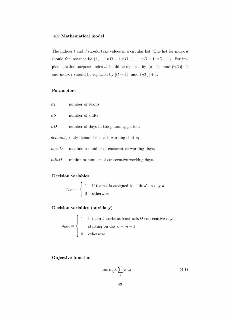
4.2 Mathematical model
The indices t and d should take values in a circular list. The list for index d
should for instance be {1, . . . , nD − 1, nD, 1, . . . , nD − 1, nD, . . .}. For im-
plementation purposes index d should be replaced by [(d−1) mod (nD)]+1
and index t should be replaced by [(t− 1) mod (nT )] + 1.
Parameters
nT number of teams;
nS number of shifts;
nD number of days in the planning period;
demands daily demand for each working shift s;
maxD maximum number of consecutive working days;
minD minimum number of consecutive working days.
Decision variables
xts′d =
1 if team t is assigned to shift s′ on day d
0 otherwise
Decision variables (auxiliary)
btdm =
1 if team t works at least minD consecutive days,
starting on day d+m− 1
0 otherwise
Objective function
min maxts
∑d
xtsd (4.1)
49
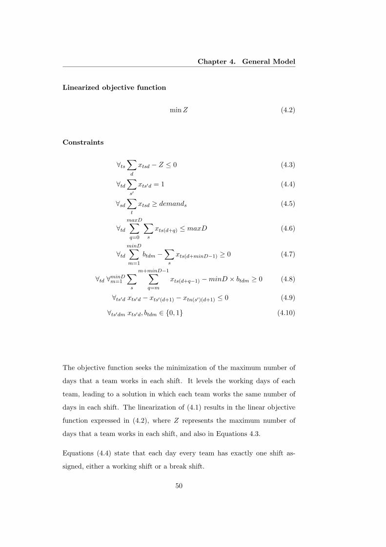
Chapter 4. General Model
Linearized objective function
minZ (4.2)
Constraints
∀ts∑d
xtsd − Z ≤ 0 (4.3)
∀td∑s′
xts′d = 1 (4.4)
∀sd∑t
xtsd ≥ demands (4.5)
∀tdmaxD∑q=0
∑s
xts(d+q) ≤ maxD (4.6)
∀tdminD∑m=1
btdm −∑s
xts(d+minD−1) ≥ 0 (4.7)
∀td ∀minDm=1
∑s
m+minD−1∑q=m
xts(d+q−1) −minD × btdm ≥ 0 (4.8)
∀ts′d xts′d − xts′(d+1) − xtn(s′)(d+1) ≤ 0 (4.9)
∀ts′dm xts′d, btdm ∈ {0, 1} (4.10)
The objective function seeks the minimization of the maximum number of
days that a team works in each shift. It levels the working days of each
team, leading to a solution in which each team works the same number of
days in each shift. The linearization of (4.1) results in the linear objective
function expressed in (4.2), where Z represents the maximum number of
days that a team works in each shift, and also in Equations 4.3.
Equations (4.4) state that each day every team has exactly one shift as-
signed, either a working shift or a break shift.
50

4.2 Mathematical model
Equations (4.5) are coverage constraints, making sure that each shift daily
requirements are fulfilled.
Equations (4.6) ensure that no team works more than maxD consecutive
days. For each day d a window of length maxD + 1 is opened and at least
one of the corresponding xtsd must be 0, independently of the working shift
s.
Days 1 2 3 4 5 6 7 8 9 10 11 12 13 14 15 16 17 18 19 20 21 22 23 24 25
Team t M M M B A A A B N N N B B M M B B A A B B N N B B
maxD+1 maxD+1 maxD+1
Figure 4.1: Illustration of Eqs. (4.6)
Equations (4.7) and (4.8) guarantee that each team works at least minD
consecutive working days. The second term on the left-hand-side of Eq.
(4.7) sums up the working days xts(d+minD−1) within a window of width
minD, starting at d. If all xts(d+minD−1) are zero no constraint is imposed
to the variables btdm. However, if at least one xts(d+minD−1) = 1 then at
least one of the variables btdm must be equal to 1. When the variable btdm
equals zero, the corresponding Eq. (4.8) is fulfilled. However if Eq. (4.7)
imposes that a variable btdm equals one, then the first term on the left-hand-
side of Eq. (4.8) has to sum-up at least minD, i.e. the team has to work
at least minD consecutive days. The meaning of m is that if a team works
one day within a window of width minD, then it has to work at least minD
consecutive days, starting at m = 1 or m = 2 or . . . or at m = minD. Figure
4.2 illustrates this process for shift M.
Equations (4.9) ensure that the required shift sequence is followed. The
basic sequencing requirement is defined over the working shifts that follow
the sequence: 1, 2, 3, 1 . . ., but, as there are breaks between the working
shifts, the breaks must carry the memory of the last working shift. This is
51

Chapter 4. General Model
Days
Team t M M M M
d
m=1 m=2 m=minD
minD
minD
minD
btd1=1 btd2=1 btdminD=1
M
Figure 4.2: Illustration of Eqs. (4.7) and (4.8)
obtained through the “extended shift” s′. For instance, if a team has an
extended shift s′ = 4 assigned, it means that the team is having a breaking
shift after a working shift 1. If the same shift is assigned on days d and d+1,
then the corresponding Eq. (4.9) is satisfied independently of the value of
xtn(s′)(d+1). However if the shift ends, i.e., a different shift is assigned on
days d and d + 1, then the next possible shift is imposed by the vector of
indices n(s′) and the Eq. (4.9). Figure 4.3 illustrates the application of Eqs.
(4.9) for the sequence of shifts defined in the example of Table 4.1.
Days 1 2 3 4 5 6 7 8
Team t M M B A B N B B
Days 1 2 3 4 5 6 7 8
Team t 1 1 4 2 5 3 6 6
Figure 4.3: Illustration of Eqs. (4.9)
52
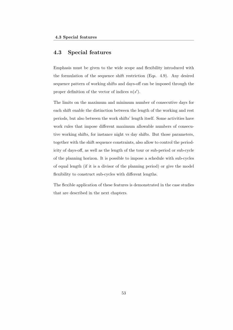
4.3 Special features
4.3 Special features
Emphasis must be given to the wide scope and flexibility introduced with
the formulation of the sequence shift restriction (Eqs. 4.9). Any desired
sequence pattern of working shifts and days-off can be imposed through the
proper definition of the vector of indices n(s′).
The limits on the maximum and minimum number of consecutive days for
each shift enable the distinction between the length of the working and rest
periods, but also between the work shifts’ length itself. Some activities have
work rules that impose different maximum allowable numbers of consecu-
tive working shifts, for instance night vs day shifts. But those parameters,
together with the shift sequence constraints, also allow to control the period-
icity of days-off, as well as the length of the tour or sub-period or sub-cycle
of the planning horizon. It is possible to impose a schedule with sub-cycles
of equal length (if it is a divisor of the planning period) or give the model
flexibility to construct sub-cycles with different lengths.
The flexible application of these features is demonstrated in the case studies
that are described in the next chapters.
53

Chapter 4. General Model
54

Chapter 5
Application of the generalmodel to a glassproduction unit
The general model presented in Chapter 4 was first adapted to the real-
life problem of a glass industry. This chapter describes that experience
and is organized as follows. Section 5.1 introduces the facility, the work
environment and the features of this particular problem. Then, in Section 5.2
the adjustments that were made to the general model are described, followed
by the achieved computational results, which are indicated in Section 5.3.
An illustration of the developed solutions is shown in Section 5.4. Section 5.5
sums up the contents of this chapter, emphasizing some important outcomes
of the work that was carried out.
5.1 Problem description
The facility produces glass bottles using two furnaces, with four lines each.
The workforce was distributed in 4 teams but the management wanted to
test the scenario of having a higher number of teams. They were convinced
this change would increase the scheduling flexibility and provide a more
55

Chapter 5. Application of the general model to a glassproduction unit
equitable schedule to all employees, in terms of workload and rest periods
distribution. Each team is a group of 36 employees that is in charge of
all the manufacturing operations during a shift. Occasional changes due to
absences of any employee are usually fulfilled within his own team.
The facility works 365 days per year, 24 hours a day, in three different
eight-hour shifts: M - morning (from 5:00 a.m. to 1:00 p.m), A - afternoon
(from 1:00 p.m. to 9:00 p.m.) and N - night (from 9:00 p.m. to 5:00 a.m.).
All teams are considered to be homogeneous in terms of skills and contract
types, everyone works full-time. Shift daily demand is fixed and known in
advance: exactly 1 team for each shift. A mandatory shifts sequence must be
respected (M-N-A) and there must be a rest shift (B) between each working
shift change (M-B-N-B-A-B). There is a predefined minimum and maximum
number of allowed consecutive working days.
5.2 Mathematical model
In order to adapt the general model to this new problem, the following
adjustments were made.
Indices
n(s′) is the extended shift that follows the extended shift s′ in a given se-
quence;
Considering the 3 working shifts {M,A,N} as {1, 2, 3} and the 3 non-
working shifts {4, 5, 6}, the sequence M-B-N-B-A-B is now defined as
shown in Table 5.1.
Parameters
δD offset between the working cycles of the teams (in number of days).
56

5.2 Mathematical model
s′ 1 2 3 4 5 6
n(s′) 4 5 6 3 1 2
Table 5.1: Sequence of shifts for the glass production unit
Constraints
∀sd∑
t xtsd = 1 (5.1)
∀nT−1t=1 ∀s′d xts′d − x(t+1)s′(d+δD) = 0 (5.2)
Equations (5.1) make sure that the daily requirements are fulfilled.
Equations (5.2) impose that all teams have the same schedule, but starting
with a time lag of δD days between them. With this additional constraint
the objective function could be replaced by a constant number but the com-
putational experiments showed that keeping the objective function lowers
the computational time. Figure 5.1 illustrates these constraints.
Days 1 2 3 4 5 6 7 8
Team 1 M M A N N Team 2 M M A N Team 3 M M A Team 4 M M
δD δD
δD
Figure 5.1: Illustration of Eqs. (5.2)
With the introduction of Eqs. (5.2), other constraints can be simplified,
reducing the size of the model. This is the case of the sequence constraints
and the maximum/minimum number of consecutive days constraints. There
is no need to apply them to all teams, it is enough to ensure that it is
fulfilled for team 1 and the offset constraint guarantees that it satisfied for
57

Chapter 5. Application of the general model to a glassproduction unit
the remaining teams. Therefore, Eqs. (4.6), (4.7), (4.8) and (4.9) were
adjusted to, respectively:
∀d∑maxD
q=0
∑s x1s(d+q) ≤ maxD (5.3)
∀d∑minD
m=1 b1dm −∑
s x1s(d+minD−1) ≥ 0 (5.4)
∀d ∀minDm=1
∑s
∑m+minD−1q=m x1s(d+q−1) −minD × b1dm ≥ 0 (5.5)
∀s′d x1s′d − x1s′(d+1) − x1n(s′)(d+1) ≤ 0 (5.6)
This approach was adopted in all the other applications of the general model,
as will be described next in this work (Chapters 6, 7 and 8).
The same analysis can be done with respect to the demand constraints (Eqs.
4.5). Theoretically, there is no need to apply them to all the nD days of
the planning period, but only to the first δD days, since the offset con-
straints ensure the fulfilment of the demand requirements for the remaining
days. However, after testing the referred simplifications, only the first group
of adjustments brought improvements to the model’s performance, reduc-
ing significantly the resolution times. Therefore, the simplification of the
demand constraints was not considered.
5.3 Computational experiments
The model was coded in OPL Studio version 6.3 and solved using the CPLEX
12.1.0 solver on a server machine powered by 2 Intel R© Xeon R© processors
of 2,4 GHz and 1,39 GHz, and with 2 GB RAM. Tests were performed con-
sidering 4 and 5 teams of employees and 3 working shifts. The maximum
(maxD) and minimum (minD) number of consecutive working days were
set to 4 and 2, respectively. A set of different planning periods and off-
sets combinations were tested. The experience showed that this problem is
58

5.4 Solutions
extremely tight in terms of relationships between parameters. There is no
place for large parameters variations and variables are strongly connected,
what makes the space of feasible solutions very limited. The only combi-
nations that always guarantee the existence of a feasible solution are those
that verify the following condition:
δD =nD
nT
The offset parameter (δD) must be equal to the ratio between the number
of days of the planning period (nD) and the number of teams (nT ). Putting
it simple, this means that the offset parameter must be the one that divides
the planning period in a number of sub-periods (or sub-cycles) equal to the
number of teams. Table 5.2 reports the computational time results and
model size, in terms of number of decision variables and constraints, for a
set of different planning periods for the 5-team scenario.
These variations were tested in order to evaluate the robustness of the model
but also to analyze the solutions built for different planning periods in order
to find the one that better fitted the objectives of the company. As expected,
the performance of the model, in terms of running time, gets worse as the
problem size increases. For 330 and 365 days the model did not generate
any feasible solution within 60000 seconds (1.7 hours).
5.4 Solutions
The solution found for a 35 days (5 weeks) planning period was achieved in
0.57 seconds (Fig. 5.2). This schedule can either be repeated as many times
as the company wants, or be integrated with schedules of other lengths, in
order to build a longer (yearly) plan. For the particular purposes of the
glass unit, the summer holidays special period was also taken into account
in a subsequent phase. Considering a planning period of 16 days, with only
59
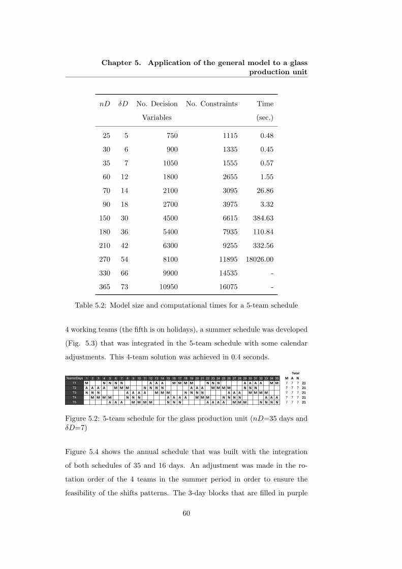
Chapter 5. Application of the general model to a glassproduction unit
nD δD No. Decision No. Constraints Time
Variables (sec.)
25 5 750 1115 0.48
30 6 900 1335 0.45
35 7 1050 1555 0.57
60 12 1800 2655 1.55
70 14 2100 3095 26.86
90 18 2700 3975 3.32
150 30 4500 6615 384.63
180 36 5400 7935 110.84
210 42 6300 9255 332.56
270 54 8100 11895 18026.00
330 66 9900 14535 -
365 73 10950 16075 -
Table 5.2: Model size and computational times for a 5-team schedule
4 working teams (the fifth is on holidays), a summer schedule was developed
(Fig. 5.3) that was integrated in the 5-team schedule with some calendar
adjustments. This 4-team solution was achieved in 0.4 seconds.
Teams/Days 1 2 3 4 5 6 7 8 9 10 11 12 13 14 15 16 17 18 19 20 21 22 23 24 25 26 27 28 29 30 31 32 33 34 35 ! " #
T1 ! ! ! # # # # ! ! ! ! " " " ! ! ! ! ! ! ! # # # ! ! ! ! " " " " ! ! ! " " " $%
T2 " " " " ! ! ! ! ! ! # # # # ! ! ! ! " " " ! ! ! ! ! ! ! # # # ! ! ! ! " " " $%
T3 # # # ! ! ! ! " " " " ! ! ! ! ! ! # # # # ! ! ! ! " " " ! ! ! ! ! ! ! " " " $%
T4 ! ! ! ! ! ! ! # # # ! ! ! ! " " " " ! ! ! ! ! ! # # # # ! ! ! ! " " " " " " $%
T5 ! ! ! ! " " " ! ! ! ! ! ! ! # # # ! ! ! ! " " " " ! ! ! ! ! ! # # # # " " " $%
&'()*
Figure 5.2: 5-team schedule for the glass production unit (nD=35 days andδD=7)
Figure 5.4 shows the annual schedule that was built with the integration
of both schedules of 35 and 16 days. An adjustment was made in the ro-
tation order of the 4 teams in the summer period in order to ensure the
feasibility of the shifts patterns. The 3-day blocks that are filled in purple
60

5.4 Solutions
Teams/Days 1 2 3 4 5 6 7 8 9 10 11 12 13 14 15 16 ! " #
T1 # # # # " " " " ! ! ! ! ! ! !
T2 ! ! # # # # " " " " ! ! ! ! !
T3 " ! ! ! ! # # # # " " " ! ! !
T4 " " " " ! ! ! ! # # # # ! ! !
$%
$%
$%
$%
&'()*
Figure 5.3: 4-team schedule for the glass production unit (nD=16 days andδD=4)
correspond to long-weekends. This problem had an additional constraint
that imposed the assignment of at least one long-weekend, for each team,
in every 5 weeks cycle. This constraint was overcome by means of a simple
calendar synchronization with the developed schedule.
The offset parameter gives a cyclic dimension to the schedule, since every
team/employee is allocated to exactly the same sequence of working shifts
and days-off, but with a time lag of δD days between each other. This feature
allows an even distribution of workload among employees, as is evidenced by
Table 5.3, which sums up the annual number of working days for each team,
for each shift and in aggregate. In this case, any unexpected adjustment to
the schedule would be done within each team of employees, having little or
no impact in the long-term schedule.
Teams/Shifts M N A Total
T1 75 72 75 222
T2 72 76 72 220
T3 75 73 73 221
T4 72 72 76 220
T5 74 75 72 221
Table 5.3: Annual number or work-days for each team
The developed model was embedded in a decision support system fitted to
the needs of the planning department of the glass production unit. The
system has a set of control flags, allowing for the user to enable all or only
61
Chapter 5. Application of the general model to a glassproduction unit
part of the constraints, as well as some quality indicators of the solution.
5.5 Conclusions
This chapter described the application of the general IP model to the real-life
problem of a glass production unit. The main adjustment was the introduc-
tion of the offset constraints (Eqs. 5.2), which ensure the workload balance
between the teams and allow for a reduction in the overall number of the
remaining constraints, improving the model’s performance. A new sequence
of shifts and days-off was imposed, by simply defining a corresponding vector
of indices n(s′). This demonstrates the flexibility of the approach developed
for the sequence constraints. Experiments focused on the evaluation of dif-
ferent optimal solutions achieved for different planning periods and allowed
for the selection of those that better suited the company’s goals, namely
in terms of holiday distribution along the year. An integrated long-term
scheduling solution was proposed, through the replication of two different
planning periods, one for the winter months and another for the summer
period. Computational times revealed the high efficiency of the model for
this particular application, which was embedded in a more complex decision
support system to be used for the glass industry management.
62

5.5 Conclusions
1/jan/10
2/jan/10
3/jan/10
4/jan/10
5/jan/10
6/jan/10
7/jan/10
8/jan/10
9/jan/10
10/jan/10
11/jan/10
12/jan/10
13/jan/10
14/jan/10
15/jan/10
16/jan/10
17/jan/10
18/jan/10
19/jan/10
20/jan/10
21/jan/10
22/jan/10
23/jan/10
24/jan/10
25/jan/10
26/jan/10
27/jan/10
28/jan/10
29/jan/10
30/jan/10
31/jan/10
1/fev/10
2/fev/10
3/fev/10
4/fev/10
5/fev/10
6/fev/10
7/fev/10
8/fev/10
9/fev/10
10/fev/10
11/fev/10
12/fev/10
13/fev/10
14/fev/10
15/fev/10
16/fev/10
17/fev/10
18/fev/10
19/fev/10
20/fev/10
21/fev/10
22/fev/10
23/fev/10
24/fev/10
25/fev/10
26/fev/10
27/fev/10
28/fev/10
1/mar/10
2/mar/10
3/mar/10
4/mar/10
5/mar/10
6/mar/10
7/mar/10
8/mar/10
9/mar/10
10/mar/10
11/mar/10
MN
A
T1
!!
!"
""
"!
##
#!
!!
!!
!!
""
"!
##
##
!!
!!
!!
""
""
!#
##
!!
!!
!!
!"
""
!#
##
#!
!!
141414
T2
##
##
!!
!!
!!
""
""
!#
##
!!
!!
!!
!"
""
!!
!!
##
##
!!
!!
!!
""
""
!#
##
!!
!!
!!
!"
""
!!
!!
141414
T3
""
"!
!!
!#
##
#!
!!
!!
!"
""
"!
##
#!
!!
!!
!!
""
"!
!!
!#
##
#!
!!
!!
!"
""
"!
##
#!
!!
!!
!!
141414
T4
!!
!!
!!
!"
""
!!
!!
##
##
!!
!!
!!
""
""
!#
##
!!
!!
!!
!"
""
!!
!!
##
##
!!
!!
!!
""
""
!#
##
141414
T5
!#
##
!!
!!
!!
!"
""
!!
!!
##
##
!!
!!
!!
""
""
!#
##
!!
!!
!!
!"
""
!!
!!
##
##
!!
!!
!!
""
""
141414
12/mar/10
13/mar/10
14/mar/10
15/mar/10
16/mar/10
17/mar/10
18/mar/10
19/mar/10
20/mar/10
21/mar/10
22/mar/10
23/mar/10
24/mar/10
25/mar/10
26/mar/10
27/mar/10
28/mar/10
29/mar/10
30/mar/10
31/mar/10
1/abr/10
2/abr/10
3/abr/10
4/abr/10
5/abr/10
6/abr/10
7/abr/10
8/abr/10
9/abr/10
10/abr/10
11/abr/10
12/abr/10
13/abr/10
14/abr/10
15/abr/10
16/abr/10
17/abr/10
18/abr/10
19/abr/10
20/abr/10
21/abr/10
22/abr/10
23/abr/10
24/abr/10
25/abr/10
26/abr/10
27/abr/10
28/abr/10
29/abr/10
30/abr/10
1/mai/10
2/mai/10
3/mai/10
4/mai/10
5/mai/10
6/mai/10
7/mai/10
8/mai/10
9/mai/10
10/mai/10
11/mai/10
12/mai/10
13/mai/10
14/mai/10
15/mai/10
16/mai/10
17/mai/10
18/mai/10
19/mai/10
20/mai/10
T1
!!
!"
""
"!
##
#!
!!
!!
!!
""
"!
##
##
!!
!!
!!
""
""
!#
##
!!
!!
!!
!"
""
!#
##
#!
!!
141414
T2
##
##
!!
!!
!!
""
""
!#
##
!!
!!
!!
!"
""
!!
!!
##
##
!!
!!
!!
""
""
!#
##
!!
!!
!!
!"
""
!!
!!
141414
T3
""
"!
!!
!#
##
#!
!!
!!
!"
""
"!
##
#!
!!
!!
!!
""
"!
!!
!#
##
#!
!!
!!
!"
""
"!
##
#!
!!
!!
!!
141414
T4
!!
!!
!!
!"
""
!!
!!
##
##
!!
!!
!!
""
""
!#
##
!!
!!
!!
!"
""
!!
!!
##
##
!!
!!
!!
""
""
!#
##
141414
T5
!#
##
!!
!!
!!
!"
""
!!
!!
##
##
!!
!!
!!
""
""
!#
##
!!
!!
!!
!"
""
!!
!!
##
##
!!
!!
!!
""
""
141414
21/mai/10
22/mai/10
23/mai/10
24/mai/10
25/mai/10
26/mai/10
27/mai/10
28/mai/10
29/mai/10
30/mai/10
31/mai/10
1/jun/10
2/jun/10
3/jun/10
4/jun/10
5/jun/10
6/jun/10
7/jun/10
8/jun/10
9/jun/10
10/jun/10
11/jun/10
12/jun/10
13/jun/10
14/jun/10
15/jun/10
16/jun/10
17/jun/10
18/jun/10
19/jun/10
20/jun/10
21/jun/10
22/jun/10
23/jun/10
24/jun/10
25/jun/10
26/jun/10
27/jun/10
28/jun/10
29/jun/10
30/jun/10
1/jul/10
2/jul/10
3/jul/10
4/jul/10
5/jul/10
6/jul/10
7/jul/10
8/jul/10
9/jul/10
10/jul/10
11/jul/10
12/jul/10
13/jul/10
14/jul/10
15/jul/10
16/jul/10
17/jul/10
18/jul/10
19/jul/10
20/jul/10
21/jul/10
22/jul/10
23/jul/10
24/jul/10
25/jul/10
26/jul/10
27/jul/10
28/jul/10
29/jul/10
T1
!!
!"
""
"!
##
#!
!!
!!
!!
""
"!
##
##
!!
!!
!"
""
"#
##
#!
!#
#111113
T2
##
##
!!
!!
!!
""
""
!#
##
!!
!!
!!
!"
""
!!
!!
##
##
!!
!!
""
""
##
##
!!
!!
""
""
151515
T3
""
"!
!!
!#
##
#!
!!
!!
!"
""
"!
##
#!
!!
!!
!!
""
""
##
##
!!
!!
""
""
##
##
!!
!!
""
"151815
T4
!!
!!
!!
!"
""
!!
!!
##
##
!!
!!
!!
""
""
!#
##
#!
!!
!"
""
"#
##
#!
!!
!"
""
"#
##
#!
161516
T5
!#
##
!!
!!
!!
!"
""
!!
!!
##
##
!!
!!
!!
""
""
!!
""
""
##
##
!!
!!
131111
30/jul/10
31/jul/10
1/ago/10
2/ago/10
3/ago/10
4/ago/10
5/ago/10
6/ago/10
7/ago/10
8/ago/10
9/ago/10
10/ago/10
11/ago/10
12/ago/10
13/ago/10
14/ago/10
15/ago/10
16/ago/10
17/ago/10
18/ago/10
19/ago/10
20/ago/10
21/ago/10
22/ago/10
23/ago/10
24/ago/10
25/ago/10
26/ago/10
27/ago/10
28/ago/10
29/ago/10
30/ago/10
31/ago/10
1/set/10
2/set/10
3/set/10
4/set/10
5/set/10
6/set/10
7/set/10
8/set/10
9/set/10
10/set/10
11/set/10
12/set/10
13/set/10
14/set/10
15/set/10
16/set/10
17/set/10
18/set/10
19/set/10
20/set/10
21/set/10
22/set/10
23/set/10
24/set/10
25/set/10
26/set/10
27/set/10
28/set/10
29/set/10
30/set/10
1/out/10
2/out/10
3/out/10
4/out/10
5/out/10
6/out/10
7/out/10
T1
##
!!
!!
""
""
##
##
!!
!!
""
""
##
##
!!
!!
""
""
!#
##
!!
!!
!!
!"
""
!#
##
#!
!!
181517
T2
""
""
##
##
!!
!!
""
""
##
##
!!
!!
""
""
!#
##
!!
!!
!!
!"
""
!!
!!
121511
T3
"#
##
#!
!!
!#
!!
!!
""
""
##
##
!!
!!
!!
""
""
!#
##
!!
!!
!!
!15912
T4
!!
!"
""
"#
##
#!
!!
!"
""
"#
##
!!
!!
##
##
!!
!!
!!
""
""
!#
##
101214
T5
""
""
##
##
!!
!!
""
""
##
##
!!
!!
""
""
##
##
!!
!!
!!
""
"!
!!
!#
##
#!
!!
!!
!"
""
"151916
8/out/10
9/out/10
10/out/10
11/out/10
12/out/10
13/out/10
14/out/10
15/out/10
16/out/10
17/out/10
18/out/10
19/out/10
20/out/10
21/out/10
22/out/10
23/out/10
24/out/10
25/out/10
26/out/10
27/out/10
28/out/10
29/out/10
30/out/10
31/out/10
1/nov/10
2/nov/10
3/nov/10
4/nov/10
5/nov/10
6/nov/10
7/nov/10
8/nov/10
9/nov/10
10/nov/10
11/nov/10
12/nov/10
13/nov/10
14/nov/10
15/nov/10
16/nov/10
17/nov/10
18/nov/10
19/nov/10
20/nov/10
21/nov/10
22/nov/10
23/nov/10
24/nov/10
25/nov/10
26/nov/10
27/nov/10
28/nov/10
29/nov/10
30/nov/10
1/dez/10
2/dez/10
3/dez/10
4/dez/10
5/dez/10
6/dez/10
7/dez/10
8/dez/10
9/dez/10
10/dez/10
11/dez/10
12/dez/10
13/dez/10
14/dez/10
15/dez/10
16/dez/10
T1
!!
!"
""
"!
##
#!
!!
!!
!!
""
"!
##
##
!!
!!
!!
""
""
!#
##
!!
!!
!!
!"
""
!#
##
#!
!!
141414
T2
##
##
!!
!!
!!
""
""
!#
##
!!
!!
!!
!"
""
!!
!!
##
##
!!
!!
!!
""
""
!#
##
!!
!!
!!
!"
""
!!
!!
141414
T3
""
"!
!!
!#
##
#!
!!
!!
!"
""
"!
##
#!
!!
!!
!!
""
"!
!!
!#
##
#!
!!
!!
!"
""
"!
##
#!
!!
!!
!!
141414
T4
!!
!!
!!
!"
""
!!
!!
##
##
!!
!!
!!
""
""
!#
##
!!
!!
!!
!"
""
!!
!!
##
##
!!
!!
!!
""
""
!#
##
141414
T5
!#
##
!!
!!
!!
!"
""
!!
!!
##
##
!!
!!
!!
""
""
!#
##
!!
!!
!!
!"
""
!!
!!
##
##
!!
!!
!!
""
""
141414
17/dez/10
18/dez/10
19/dez/10
20/dez/10
21/dez/10
22/dez/10
23/dez/10
24/dez/10
25/dez/10
26/dez/10
27/dez/10
28/dez/10
29/dez/10
30/dez/10
31/dez/10
1/jan/11
2/jan/11
3/jan/11
T1
!!
!"
""
"!
##
#!
!!
!4
43
T2
##
##
!!
!!
!!
""
""
!3
44
T3
""
"!
!!
!#
##
#!
!!
!!
!"
34
4
T4
!!
!!
!!
!"
""
!!
!!
##
##
43
4
T5
!#
##
!!
!!
!!
!"
""
!4
33
Fig
ure
5.4:
Ann
ual
sche
dule
for
the
glas
spr
oduc
tion
unit
63

Chapter 5. Application of the general model to a glassproduction unit
64
Chapter 6
Application of the generalmodel to a continuous careunit
The general model described in Chapter 4 was in a second phase adapted to
the real-world problem of a continuous care unit. This chapter presents that
work and is organized as follows. Section 6.1 introduces the service type,
the work environment and the features of this particular problem. Then, in
Section 6.2 the adjustments that were made to the general model are ex-
plained, followed by the achieved computational results, which are presented
in Section 6.3. A proposed solution is shown in Section 6.4. Section 6.5 re-
sumes this chapter, highlighting some important outcomes of the developed
research work.
6.1 Problem description
The organization provides private lodging and nursing home services, di-
rected mainly to the elderly. This work addresses the scheduling of only
part of the workforce that is composed by care takers, which are employees
with no specific qualifications that are responsible for the daily basic needs
65
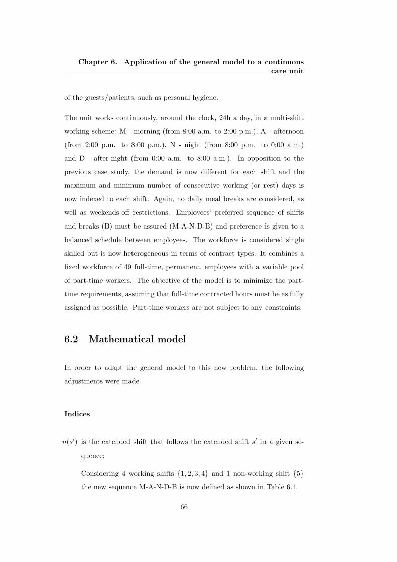
Chapter 6. Application of the general model to a continuouscare unit
of the guests/patients, such as personal hygiene.
The unit works continuously, around the clock, 24h a day, in a multi-shift
working scheme: M - morning (from 8:00 a.m. to 2:00 p.m.), A - afternoon
(from 2:00 p.m. to 8:00 p.m.), N - night (from 8:00 p.m. to 0:00 a.m.)
and D - after-night (from 0:00 a.m. to 8:00 a.m.). In opposition to the
previous case study, the demand is now different for each shift and the
maximum and minimum number of consecutive working (or rest) days is
now indexed to each shift. Again, no daily meal breaks are considered, as
well as weekends-off restrictions. Employees’ preferred sequence of shifts
and breaks (B) must be assured (M-A-N-D-B) and preference is given to a
balanced schedule between employees. The workforce is considered single
skilled but is now heterogeneous in terms of contract types. It combines a
fixed workforce of 49 full-time, permanent, employees with a variable pool
of part-time workers. The objective of the model is to minimize the part-
time requirements, assuming that full-time contracted hours must be as fully
assigned as possible. Part-time workers are not subject to any constraints.
6.2 Mathematical model
In order to adapt the general model to this new problem, the following
adjustments were made.
Indices
n(s′) is the extended shift that follows the extended shift s′ in a given se-
quence;
Considering 4 working shifts {1, 2, 3, 4} and 1 non-working shift {5}
the new sequence M-A-N-D-B is now defined as shown in Table 6.1.
66

6.2 Mathematical model
s′ 1 2 3 4 5
n(s′) 2 3 4 5 1
Table 6.1: Sequence of shifts for the continuous care unit
maxDs′ maximum number of consecutive working (shifts 1 to 4) and rest
(shift 5) days for each shift;
minDs′ minimum number of consecutive working (shifts 1 to 4) and rest
(shift 5) days for each shift;
ptCosts hourly cost of a part-time employee working in shift s;
hs number of working hours of shift s.
Parameters
δD offset between the working cycles of the teams (in number of days).
Objective function Minimization of the cost with part-time work.
min∑
d
∑s ptCosts × hs × (demands −
∑t xtsd) (6.1)
Constraints
∀sd∑t
xtsd ≤ demands (6.2)
Equations (6.2) state that each day, the number of full-time employees as-
signed to every working shift is less than or equal to the demand. The
difference between the assigned and the demanded work will be assured by
part-time workers.
The cyclic approach introduced in Chapter 5 was also adopted in this for-
mulation. Therefore, the model constraints include Eqs. (5.2), (5.3), (5.4),
67

Chapter 6. Application of the general model to a continuouscare unit
(5.5) and (5.6). See Section 5.2 for a detailed description of each one of the
equations.
Equations (5.3), (5.4), (5.5) were adjusted to consider extended shifts, which
implied the replacement of the parameters maxD and minD by the indexed
parameters maxDs′ and minDs′ . These represent minor adjustments, but
in order to allow for an easier reading the new Eqs. (6.3), (6.4) and (6.5)
are presented next.
∀s′d∑maxDs′
q=0 x1s′(d+q) ≤ maxDs′ (6.3)
∀s′d∑minDs′
m=1 b1dm − x1s′(d+minDs′−1) ≥ 0 (6.4)
∀s′d ∀minDs′m=1
∑m+minDs′−1q=m x1s′(d+q−1) −minDs′ × b1dm ≥ 0 (6.5)
6.3 Computational experiments
The model was coded in OPL Studio version 6.3 and solved using the CPLEX
12.1.0 solver on a server machine powered by 2 Intel R© Xeon R© processors
of 2,4 GHz and 1,39 GHz, and with 2 GB RAM. The number of employees
(nT ) is 49 and the working shifts (nS) are now 4. The daily shift demand
(demands) is 20 M, 17 A, 11 N and 11 D. Tests were conducted for planning
periods of 25, 28 and 30 days, considering different combinations of the
parameters minDs′ , maxDs′ and ptCosts. The choice of the values of these
parameters took into account the desired length of the sub-periods, the
assurance of the minimum of one day-off every 7 days, and also that the
working hours assigned to each employee should fall below 160h in a 30-
day period in order to respect labor contracts. The reasoning made in the
previous case study, concerning the value of the offset parameter, does not
make sense in this problem, since the planning period is now shorter than
the number of employees. Therefore, the offset was set to 1, as it achieved
satisfactory results.
68

6.3 Computational experiments
In terms of dimension, the number of decision variables of this problem
varies between 6125 for nD=25 and 7350 for nD=30 and the number of
constraints reaches the maximum of 8250 for nD=30 and maxD1 = maxD2
= 3, maxD3 = maxD4 = maxD5 = 1.
Table 6.2 reports the computational results for a set of different values of
input parameters. The column ”solution pattern” contains the schedule for
one employee for the whole planning period considered, as illustrated in the
next examples. Figures 6.1 and 6.2 show the schedule for E1 in a nD = 25
days scenario.
!" # $ % & ' ( ) * + #, ## #$ #% #& #' #( #) #* #+ $, $# $$ $% $& $'
-# . . / / 0 " 1 . . / / 0 " 1 . . / 0 " 1 . / 0 " 1
Figure 6.1: Schedule of E1 for nD=25 days; maxD1 = maxD2 = 2 andmaxD3 = maxD4 = maxD5 = 1; minD1 = minD2 = minD3 = minD4 =minD5 = 1; ptCost1 = ptCost2 = ptCost3 = ptCost4 = 1.
nD 1 2 3 4 5 6 7 8 9 10 11 12 13 14 15 16 17 18 19 20 21 22 23 24 25E1 M A N D F M A N D F M A N D F M A N D F M A N D F
Figure 6.2: Schedule of E1 for nD=25 days; maxD1 = maxD2 = maxD3
= maxD4 = maxD5 = 1; minD1 = minD2 = minD3 = minD4 = minD5
= 1; ptCost1 = ptCost2 = ptCost3 = ptCost4 = 1.
The ability to control the solution pattern with the variation of input pa-
rameters is noticeable. For this scenario, for example, it is possible to get
a balanced solution, with sub-periods of equal length, with a reduction of
maxDs′ , forcing the model to assign exactly 1 day to each shift. In this
solution the number of sub-periods increases from 4 in Fig. 6.1 to 5 in
Fig. 6.2, meaning that the number of breaks or days-off of full-time em-
ployees will also increase, as well as the requirements for part-time service
(higher/poorer solution value).
The results of the tuning of maxDs′ and minDs′ can also be checked for
a 30 days planning horizon. In this case, fixing to 2 the minimum number
69

Chapter 6. Application of the general model to a continuouscare unit
nD
maxD
sm
inD
sptC
osts
Solu
tion
Pattern
PT
Req
.
s=
MA
ND
Bs
=M
AN
DB
s=
MA
ND
(sub-p
eriods)
(hours)
25
22
11
11
11
11
11
11
MM
AA
ND
B-M
MA
AN
DB
-MM
AN
DB
-MA
ND
B2676
25
11
11
11
11
11
11
11
MA
ND
B-M
AN
DB
-MA
ND
B-M
AN
DB
-MA
ND
B2970
28
33
11
11
11
11
11
11
MM
MA
AN
DB
-MM
AA
ND
B-M
MA
AA
ND
B-M
AN
DB
2856
28
22
11
11
11
11
11
11
MM
AA
ND
B-M
MA
AN
DB
-MM
AA
ND
B-M
MA
AN
DB
2856
28
22
11
11
11
11
11
33
MA
AN
DB
-MA
ND
B-M
AA
ND
B-M
AN
DB
-MA
AN
DB
3150
28
22
11
11
11
11
15
1000
1000
MA
AN
DB
-MA
ND
B-M
AA
ND
B-M
AA
ND
B-M
AN
DB
3150
30
33
11
11
11
11
11
11
MM
MA
ND
B-M
MM
AA
ND
B-M
MM
AN
DB
-MM
AA
AN
DB
2976
30
22
11
11
11
11
11
11
MA
ND
B-M
AN
DB
-MA
AN
DB
-MM
AA
ND
B-M
MA
AN
DB
3270
30
21
11
12
11
11
11
11
MM
AN
DB
-MM
AN
DB
-MM
AN
DB
-MM
AN
DB
-MM
AN
DB
3270
30
11
11
11
11
11
11
11
MA
ND
B-M
AN
DB
-MA
ND
B-M
AN
DB
-MA
ND
B-M
AN
DB
3564
30
33
11
11
11
11
11
1000
1000
MA
ND
B-M
AN
DB
-MA
ND
B-M
AN
DB
-MA
ND
B-M
AN
DB
3564
Table
6.2:M
odelcom
putationalparam
etersand
resultsfor
thecontinuous
careunit
70

6.3 Computational experiments
of consecutive days of shift M, results in a balanced solution but with the
same number of sub-periods and, therefore, with the same solution value.
Figures 6.3 and 6.4 illustrate this example.
nD 1 2 3 4 5 6 7 8 9 10 11 12 13 14 15 16 17 18 19 20 21 22 23 24 25 26 27 28 29 30E1 M A N D F M A N D F M A A N D F M M A A N D F M M A A N D F
Figure 6.3: Schedule of E1 for nD=30 days; maxD2 = maxD2 = 2 andmaxD3 = maxD4 = maxD5 = 1; minD1 = minD2 = minD3 = minD4 =minD5 = 1; ptCost1 = ptCost2 = ptCost3 = ptCost4 = 1.
nD 1 2 3 4 5 6 7 8 9 10 11 12 13 14 15 16 17 18 19 20 21 22 23 24 25 26 27 28 29 30E1 M M A N D F M M A N D F M M A N D F M M A N D F M M A N D F
Figure 6.4: Schedule of E1 for nD=30 days; maxD1 = 2 and maxD2 =maxD3 = maxD4 = maxD5 = 1; minD1 = 2 and minD2 = minD3 =minD4 = minD5 = 1; ptCost1 = ptCost2 = ptCost3 = ptCost4 = 1.
The influence of the ptCosts parameter can be verified in the 28 days plan-
ning horizon case. The increase from 1 (Fig. 6.5) to 3 (Fig. 6.6) units,
results in a higher number of sub-periods and therefore, in a higher number
of days-off of full time employees and higher part-time needs, leading to a
worse solution.
!" # $ % & ' ( ) * + #, ## #$ #% #& #' #( #) #* #+ $, $# $$ $% $& $' $( $) $*
-# . . / / 0 " 1 . . / / 0 " 1 . . / / 0 " 1 . . / / 0 " 1
Figure 6.5: Schedule of E1 for nD=28 days; maxD1 = maxD2 = 2 andmaxD3 = maxD4 = maxD5 = 1; minD1 = minD2 = minD3 = minD4 =minD5 = 1; ptCost1 = ptCost2 = ptCost3 = ptCost4 = 1.
The same happens in the nD=30 case, where an increase from 1 (Fig. 6.7)
to 1000 (Fig. 6.8), in the hourly cost of the part-time night and after-night
shifts, achieves a solution with 2 additional sub-periods, which means more
part-time requirements and consequently a worse solution value. In terms
of execution times, each run took less than 4 seconds.
71

Chapter 6. Application of the general model to a continuouscare unit
!" # $ % & ' ( ) * + #, ## #$ #% #& #' #( #) #* #+ $, $# $$ $% $& $' $( $) $*
-# . / / 0 " . / 0 " . / / 0 " . / 0 " . / / 0 "
Figure 6.6: Schedule of E1 for nD=30 days; maxD1 = maxD2 = 2 andmaxD3 = maxD4 = maxD5 = 1; minD1 = minD2 = minD3 = minD4 =minD5 = 1; ptCost1 = ptCost2 = 1 and ptCost3 = ptCost4 = 3.
!" # $ % & ' ( ) * + #, ## #$ #% #& #' #( #) #* #+ $, $# $$ $% $& $' $( $) $* $+ %,
-# . . . / / 0 " 1 . . . / / 0 " 1 . . . / 0 " 1 . . / / 0 " 1
Figure 6.7: Schedule of E1 for nD=30 days; maxD1 = maxD2 = 3 andmaxD3 = maxD4 = maxD5 = 1; minD1 = minD2 = minD3 = minD4 =minD5 = 1; ptCost1 = ptCost2 = ptCost3 = ptCost4 = 1.
nD 1 2 3 4 5 6 7 8 9 10 11 12 13 14 15 16 17 18 19 20 21 22 23 24 25 26 27 28 29 30E1 M A N D F M A N D F M A N D F M A N D F M A N D F M A N D F
Figure 6.8: Schedule of E1 for nD=30 days; maxD1 = maxD2 = 3 andmaxD3 = maxD4 = maxD5 = 1; minD1 = minD2 = minD3 = minD4 =minD5 = 1; ptCost1 = ptCost2 = 1 and ptCost3 = ptCost4 = 1000.
6.4 Solutions
Figure 6.9 shows the schedule for nD=28 days, maxD1 = maxD2 = 2,
maxD3 = maxD4 = maxD5 = 1, minD1 = minD2 = minD3 = minD4 =
minD5 = 1 and ptCost1 = ptCost2 = ptCost3 = ptCost4 = 1. With this
solution, which was obtained in 2.6 seconds, the number of required part-
time shifts is 476, corresponding to a total of 2856 hours. According to this
schedule, each employee has 144 hours of work assigned in a 28 days period.
In fact, this is very close to the target of 160 hours in a 30-days period.
6.5 Conclusions
The problem of the continuous care unit highlighted the challenge of adapt-
ing the general IP model to a service environment and more specifically to
the hospitality sector. The introduction of part-time workers called for an
adjustment in the objective function, which now sought to minimize part-
72
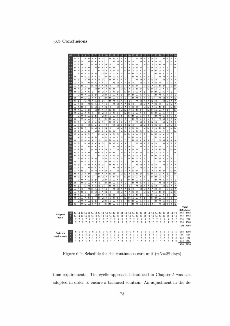
6.5 Conclusions
!""#$%&'(
)*+,"
-.,/0/#1&(
,&2+#,&1&%/"
!" # $ % & ' ( ) * + #, ## #$ #% #& #' #( #) #* #+ $, $# $$ $% $& $' $( $) $*
-# . " / 0 0 1 1 . " / 0 0 1 1 . " / 0 0 1 1 . " / 0 0 1 1
-$ 1 . " / 0 0 1 1 . " / 0 0 1 1 . " / 0 0 1 1 . " / 0 0 1
-% 1 1 . " / 0 0 1 1 . " / 0 0 1 1 . " / 0 0 1 1 . " / 0 0
-& 0 1 1 . " / 0 0 1 1 . " / 0 0 1 1 . " / 0 0 1 1 . " / 0
-' 0 0 1 1 . " / 0 0 1 1 . " / 0 0 1 1 . " / 0 0 1 1 . " /
-( / 0 0 1 1 . " / 0 0 1 1 . " / 0 0 1 1 . " / 0 0 1 1 . "
-) " / 0 0 1 1 . " / 0 0 1 1 . " / 0 0 1 1 . " / 0 0 1 1 .
-* . " / 0 0 1 1 . " / 0 0 1 1 . " / 0 0 1 1 . " / 0 0 1 1
-+ 1 . " / 0 0 1 1 . " / 0 0 1 1 . " / 0 0 1 1 . " / 0 0 1
-#, 1 1 . " / 0 0 1 1 . " / 0 0 1 1 . " / 0 0 1 1 . " / 0 0
-## 0 1 1 . " / 0 0 1 1 . " / 0 0 1 1 . " / 0 0 1 1 . " / 0
-#$ 0 0 1 1 . " / 0 0 1 1 . " / 0 0 1 1 . " / 0 0 1 1 . " /
-#% / 0 0 1 1 . " / 0 0 1 1 . " / 0 0 1 1 . " / 0 0 1 1 . "
-#& " / 0 0 1 1 . " / 0 0 1 1 . " / 0 0 1 1 . " / 0 0 1 1 .
-#' . " / 0 0 1 1 . " / 0 0 1 1 . " / 0 0 1 1 . " / 0 0 1 1
-#( 1 . " / 0 0 1 1 . " / 0 0 1 1 . " / 0 0 1 1 . " / 0 0 1
-#) 1 1 . " / 0 0 1 1 . " / 0 0 1 1 . " / 0 0 1 1 . " / 0 0
-#* 0 1 1 . " / 0 0 1 1 . " / 0 0 1 1 . " / 0 0 1 1 . " / 0
-#+ 0 0 1 1 . " / 0 0 1 1 . " / 0 0 1 1 . " / 0 0 1 1 . " /
-$, / 0 0 1 1 . " / 0 0 1 1 . " / 0 0 1 1 . " / 0 0 1 1 . "
-$# " / 0 0 1 1 . " / 0 0 1 1 . " / 0 0 1 1 . " / 0 0 1 1 .
-$$ . " / 0 0 1 1 . " / 0 0 1 1 . " / 0 0 1 1 . " / 0 0 1 1
-$% 1 . " / 0 0 1 1 . " / 0 0 1 1 . " / 0 0 1 1 . " / 0 0 1
-$& 1 1 . " / 0 0 1 1 . " / 0 0 1 1 . " / 0 0 1 1 . " / 0 0
-$' 0 1 1 . " / 0 0 1 1 . " / 0 0 1 1 . " / 0 0 1 1 . " / 0
-$( 0 0 1 1 . " / 0 0 1 1 . " / 0 0 1 1 . " / 0 0 1 1 . " /
-$) / 0 0 1 1 . " / 0 0 1 1 . " / 0 0 1 1 . " / 0 0 1 1 . "
-$* " / 0 0 1 1 . " / 0 0 1 1 . " / 0 0 1 1 . " / 0 0 1 1 .
-$+ . " / 0 0 1 1 . " / 0 0 1 1 . " / 0 0 1 1 . " / 0 0 1 1
-%, 1 . " / 0 0 1 1 . " / 0 0 1 1 . " / 0 0 1 1 . " / 0 0 1
-%# 1 1 . " / 0 0 1 1 . " / 0 0 1 1 . " / 0 0 1 1 . " / 0 0
-%$ 0 1 1 . " / 0 0 1 1 . " / 0 0 1 1 . " / 0 0 1 1 . " / 0
-%% 0 0 1 1 . " / 0 0 1 1 . " / 0 0 1 1 . " / 0 0 1 1 . " /
-%& / 0 0 1 1 . " / 0 0 1 1 . " / 0 0 1 1 . " / 0 0 1 1 . "
-%' " / 0 0 1 1 . " / 0 0 1 1 . " / 0 0 1 1 . " / 0 0 1 1 .
-%( . " / 0 0 1 1 . " / 0 0 1 1 . " / 0 0 1 1 . " / 0 0 1 1
-%) 1 . " / 0 0 1 1 . " / 0 0 1 1 . " / 0 0 1 1 . " / 0 0 1
-%* 1 1 . " / 0 0 1 1 . " / 0 0 1 1 . " / 0 0 1 1 . " / 0 0
-%+ 0 1 1 . " / 0 0 1 1 . " / 0 0 1 1 . " / 0 0 1 1 . " / 0
-&, 0 0 1 1 . " / 0 0 1 1 . " / 0 0 1 1 . " / 0 0 1 1 . " /
-&# / 0 0 1 1 . " / 0 0 1 1 . " / 0 0 1 1 . " / 0 0 1 1 . "
-&$ " / 0 0 1 1 . " / 0 0 1 1 . " / 0 0 1 1 . " / 0 0 1 1 .
-&% . " / 0 0 1 1 . " / 0 0 1 1 . " / 0 0 1 1 . " / 0 0 1 1
-&& 1 . " / 0 0 1 1 . " / 0 0 1 1 . " / 0 0 1 1 . " / 0 0 1
-&' 1 1 . " / 0 0 1 1 . " / 0 0 1 1 . " / 0 0 1 1 . " / 0 0
-&( 0 1 1 . " / 0 0 1 1 . " / 0 0 1 1 . " / 0 0 1 1 . " / 0
-&) 0 0 1 1 . " / 0 0 1 1 . " / 0 0 1 1 . " / 0 0 1 1 . " /
-&* / 0 0 1 1 . " / 0 0 1 1 . " / 0 0 1 1 . " / 0 0 1 1 . "
-&+ " / 0 0 1 1 . " / 0 0 1 1 . " / 0 0 1 1 . " / 0 0 1 1 .
")#3/" )*+,"
0 #& #& #& #& #& #& #& #& #& #& #& #& #& #& #& #& #& #& #& #& #& #& #& #& #& #& #& #& %+$ $%'$
1 #& #& #& #& #& #& #& #& #& #& #& #& #& #& #& #& #& #& #& #& #& #& #& #& #& #& #& #& %+$ $%'$
. ) ) ) ) ) ) ) ) ) ) ) ) ) ) ) ) ) ) ) ) ) ) ) ) ) ) ) ) #+( )*&
" ) ) ) ) ) ) ) ) ) ) ) ) ) ) ) ) ) ) ) ) ) ) ) ) ) ) ) ) #+( #'(*
4456 5786
0 ( ( ( ( ( ( ( ( ( ( ( ( ( ( ( ( ( ( ( ( ( ( ( ( ( ( ( ( #(* #,,*
1 % % % % % % % % % % % % % % % % % % % % % % % % % % % % *& ',&
. & & & & & & & & & & & & & & & & & & & & & & & & & & & & ##$ &&*
" & & & & & & & & & & & & & & & & & & & & & & & & & & & & ##$ *+(
956 :;86
<*/.=
Figure 6.9: Schedule for the continuous care unit (nD=28 days)
time requirements. The cyclic approach introduced in Chapter 5 was also
adopted in order to ensure a balanced solution. An adjustment in the de-
73

Chapter 6. Application of the general model to a continuouscare unit
mand constraints (Eqs. 4.5, 6.2) was made in order to consider an upper
bound for the number of assigned full-time workers. The number of consecu-
tive days-off was now limited to a minimum and a maximum value, requiring
an extension of Eqs. (5.3), (5.4) and (5.5) to consider extended shifts (index
s′). A new different sequence of shifts and days-off was imposed, by simply
defining a new vector of indices n(s′). Again, the flexibility of the approach
developed for the sequence constraints was demonstrated. Experiments fo-
cused on the evaluation of different optimal solutions achieved for three
planning periods: 25, 28 and 30 days. Computational results prove the effi-
ciency of the model. Several scenarios were tested in a few seconds and their
impact in terms of different indicators were analyzed. A sensitivity analysis
to the variation of the parameters maxDs′ , minDs′ and ptCosts was made
in Section 6.3, demonstrating the potentials of the proposed formulation.
The tuning of those parameters allows for differentiating the length of each
block of working shifts and days-off and therefore for controlling the length
of the patterns of working shifts and days-off. A schedule built for a period
of 28 days was presented. Although it was not implemented in real context,
the model was adjusted to consider the real features and restrictions of the
problem, as reported by the continuous care unit. All the input data for the
experiments were also provided by the organization.
74

Chapter 7
Application of the generalmodel to a hospital
This chapter describes the application of the general IP model introduced in
Chapter 4 to a hospital unit. This is a real problem of nurse scheduling in the
general surgery service of a Portuguese hospital that was addressed before
in Antunes and Moz (2011). Section 7.1 presents the work environment
and the features of this particular problem. The adjustments that were
made to the general model are explained in Section 7.2. Next, the achieved
computational results and proposed solutions are presented in Section 7.3.
Section 7.4 closes this chapter.
7.1 Problem description
As in any hospital, this general surgery unit works continuously 24 hours
a day. Three work shifts are considered: M - morning (from 8:00 a.m. to
4:00 p.m.), A - afternoon (from 3:30 p.m. to 11:00 p.m.) and N - night
(from 11:30 p.m. to 8:30 a.m.). There are also 2 rest shifts to take into
account: D and B. In each week (7 days), at least two of the days must
be assigned to shifts D and/or B and the nurses cannot work more than 6
75

Chapter 7. Application of the general model to a hospital
consecutive days. The preferred sequence of shifts is M-M-T-T-D-N-N-B.
The daily requirements of each working shift are limited by a minimum and
a maximum number of nurses, as presented in Table 7.1.
Shift / Day Mon Tue Wed Thu Fri Sat Sun
M 12/13 12/12 13/13 12/13 13/13 8/9 8/9
T 7/8 8/8 8/8 8/8 8/9 7/8 7/8
N 6/7 6/7 6/7 6/7 6/7 6/7 6/7
Table 7.1: Minimum/maximum no. of nurses required daily for each shift
The workforce is composed by 42 nurses with 5 different contract types,
distributed as presented in Table 7.2.
Type of contract No. of nurses No. of contracted hours/ week
1 5 42
2 31 40
3 2 33
4 2 32
5 2 31
Table 7.2: Types of contracts
The objective is to assign a number of hours to each nurse as close as possible
to the contracted ones.
7.2 Mathematical model
In order to adapt the general model to this new problem, the following
adjustments were made.
Indices
76

7.2 Mathematical model
n(s′) is the extended shift that follows the extended shift s′ in a given se-
quence;
Considering 3 working shifts {1, 2, 3} and 2 non-working shifts {4, 5}
the preferred sequence M-M-A-A-D-N-N-B can be represented as dis-
played in Table 7.3.
s′ 1 2 3 4 5
n(s′) 2 4 5 3 1
Table 7.3: Sequence of shifts for the hospital problem
k ∈ {1, 2, 3, 4, 5}, type of nurse (or contract);
maxDks′ maximum number of consecutive working (shifts 1 to 3) and rest
(shifts 4 and 5) days for each shift and for each type of nurse k;
minDks′ minimum number of consecutive working (shifts 1 to 3) and rest
(shifts 4 and 5) days for each shift and for each type of nurse k;
ps number of hours of each working shift s;
at balance of worked vs contracted hours of nurse t in the previous plan-
ning period;
ht number of contracted working hours of nurse t in the planning period
nD; depends on the type of contract;
dMinsd minimum number of nurses required in each shift s, in each day d;
dMaxsd maximum number of nurses required in each shift s, in each day d;
w time window (days).
Objective function Minimization of the difference between contracted
and assigned working hours.
77

Chapter 7. Application of the general model to a hospital
min∑
t |[(ht − at)−∑
s
∑d(ps × xtsd)]| (7.1)
Constraints
∀sd∑
t xtsd ≥ dMinsd (7.2)
∀sd∑
t xtsd ≤ dMaxsd (7.3)
Equations (7.2) and (7.3) state that each day, the required number of work-
ing nurses for each shift is ensured.
∀td∑w−1
i=0
∑5s′=4 xts′(d+i) ≥ 2 (7.4)
Equation (7.4) imposes a minimum of two non-working days (D or B) in
each window w.
The cyclic approach introduced in Chapter 5 was once more adopted. The
model constraints include Eqs. (5.2), (5.3), (5.4), (5.5) and (5.6). See Sec-
tion 5.2 for a detailed description.
Equations (5.3), (5.4), (5.5) were adjusted to consider the indexed parame-
ters maxDks′ and minDks′ . These parameters can be set to different values
in order to evaluate different patterns for the sequence of shifts of the differ-
ent types of contracts. These represent minor adjustments, but in order to
allow for an easier reading the new Eqs. (7.5), (7.6) and (7.7) are presented
next.
∀ks′d∑maxDks′
q=0 x1s′(d+q) ≤ maxDks′ (7.5)
∀ks′d∑minDks′
m=1 b1dm − x1s′(d+minDks′−1) ≥ 0 (7.6)
∀ks′d ∀minDks′m=1
∑m+minDks′−1q=m x1s′(d+q−1) −minDks′ × b1dm ≥ 0 (7.7)
78

7.3 Computational experiments and solutions
The scheduling constraints that ensure a maximum of 6 consecutive work
days for each nurse are imposed by the tuning of the parameters maxDks′
and minDks′ .
7.3 Computational experiments and solutions
The model was coded in OPL Studio version 6.3 and solved using the CPLEX
12.1.0 solver on a server machine powered by 2 Intel R© Xeon R© processors of
2,4 GHz and 1,39 GHz, and with 2 GB RAM. In this problem the workforce
is composed by 42 nurses with different contract types. For implementation
purposes, the 42 nurses were divided in 5 groups, as shown in Fig. 7.4.
t Type of contract
1. . . 5 1
6. . . 36 2
37. . . 38 3
39. . . 40 4
41. . . 42 5
Table 7.4: Association of index t to the type of contract
Since each type of contract is linked to a number of contracted hours, each
nurse is thus initially connected to a number of contracted hours per plan-
ning period. This approach led to a lower number of decision variables than
the alternative of indexing each decision variable to a nurse. In opposition to
the previous case studies, as there are nurses with different contracted hours,
it was not reasonable to impose the same offset to all the schedules. There-
fore, each group of nurses of the same type had its own offset. In terms of
size, this model dealt with 5880 decision variables and 952 constraints. Just
to give an idea of the influence of the offset constraints in the simplification
of the model, if these constraints were not considered the overall number of
79

Chapter 7. Application of the general model to a hospital
constraints would be 37 times higher, increasing from 952 to 35392. Fig-
ure 7.1 shows a solution obtained for this case study in 1170.9 seconds (20
minutes). In this case, maxDks′ = 5 for k=1,. . . ,5 and s′=1,. . . ,4; maxD15
= maxD25 = 5 and maxD35 = maxD45 = maxD55 = 7; minDks′ = 1, for
k=1,. . . ,5 and s′=1,. . . ,5.
The formulation of the parameters maxDks′ and minDks′ allows us to con-
trol the relation between the number of work and rest days for each type
of nurse. In this case, it makes sense to allow for more breaks for those
nurse types that have less contracted work hours (maxD35 = maxD45 =
maxD55 = 7).
This solution does not consider planned absences or holidays. Although
this constraint has not been treated in the previous applications of the IP
model, we decided to introduce it in the hospital case study since it was
addressed in the solution proposed in the original work of Antunes and Moz
(2011) and, therefore, it makes the comparison between approaches easier
and more realistic. In order to consider this scenario, the decision variables
corresponding to each planned day-off were initially set to 0 and the offset
constraints could not be applied to the teams that had planned days-off.
Sequence and maximum/minimum consecutive days constraints were also
adjusted individually for each of those teams in order to exclude the days-off.
Figure 7.2 shows the solution obtained when considering the planned days-
off for this particular month. As expected, the execution time increased, as
the model gets more constrained, and it takes now 2256.3 seconds (about
38 minutes) to obtain this solution.
80
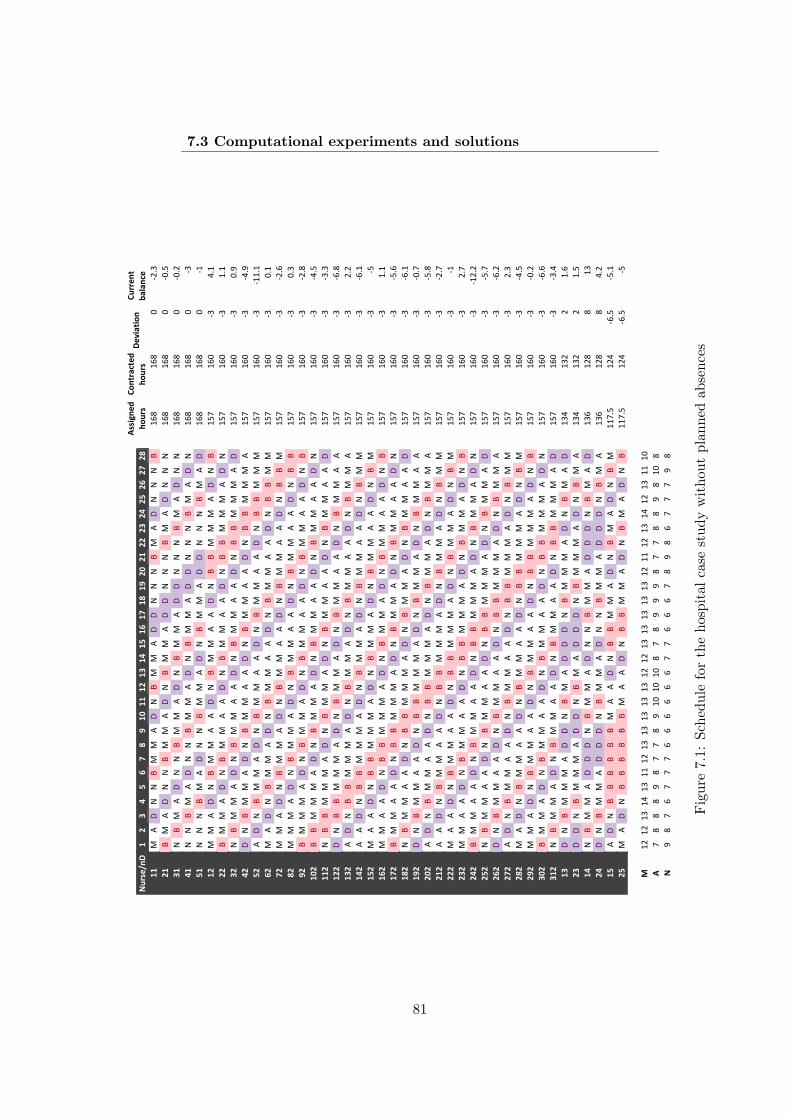
7.3 Computational experiments and solutions!"#$%&'(
))
*)
+)
,)
-)
)*
**
+*
,*
-*
.*
/*
0*
1*
)2*
))*
)**
)+*
),*
)-*
).*
)/*
)0*
)1*
*2*
*)*
***
*+*
*,*
*-*
*.*
*/*
*0*
*1*
+2*
+)*
)+
*+
),
*,
)-
*-
3 4 !
)*
+,
-.
/0
1)2
))
)*
)+
),
)-
).
)/
)0
)1
*2
*)
**
*+
*,
*-
*.
*/
*0
!"
#$
$%
!!
"#
$%
!!
"#
#$
$$
%!
"#
$$
$%
%!
"#
$$
%!
!"
#$
%!
!"
##
$$
$%
!"
#$
$$
$%
!"
#$
$%
!!
"#
$%
!!
"#
#$
$$
%!
"#
$$
$$
%!
"#
$$
%!
!"
#$
%!
!"
##
$$
$%
!"
#$
$$
$%
!"
#$
$%
!!
"#
$%
!!
"#
#$
$$
%!
"#
!!
"#
$%
!!
""
#$
%!
!"
"#
$%
%!
!!
"#
$%
%!
!"
#$
%!
!"
"#
$%
!!
""
#$
%%
!!
!"
#$
$%
!!
"#
$%
!!
""
#$
%!
!"
"#
$%
%!
!!
"#
#$
%!
!"
#$
%!
!"
"#
$%
!!
""
#$
%%
!!
!"
"#
$%
!!
"#
$%
!!
""
#$
%!
!"
"#
$%
%!
!!
!"
#$
%!
!"
#$
%!
!"
"#
$%
!!
""
#$
%%
!!
!!
"#
$%
!!
"#
$%
!!
""
#$
%!
!"
"#
$%
%!
!!
!"
#$
%!
!"
#$
%!
!"
"#
$%
!!
""
#$
%%
%!
!!
"#
$%
!!
"#
$%
!!
""
#$
%!
!"
"#
$%
%%
!!
!"
#$
%!
!"
#$
%!
!"
"#
$%
!!
""
#$
$%
%!
!!
"#
$%
!!
"#
$%
!!
""
#$
%!
!"
"#
#$
%%
!!
!"
#$
%!
!"
#$
%!
!"
"#
$%
!!
""
"#
$%
%!
!!
"#
$%
!!
"#
$%
!!
""
#$
%!
!"
""
#$
%%
!!
!"
#$
%!
!"
#$
%!
!"
"#
$%
!!
!"
"#
$%
%!
!!
"#
$%
!!
"#
$%
!!
""
#$
%!
!!
""
#$
%%
!!
!"
#$
%!
!"
#$
%!
!"
"#
$%
%!
!"
"#
$%
%!
!!
"#
$%
!!
"#
$%
!!
""
#$
$%
!!
""
#$
%%
!!
!"
#$
%!
!"
#$
%!
!"
"#
#$
%!
!"
"#
$%
%!
!!
"#
$%
!!
"#
$%
!!
""
"#
$%
!!
""
#$
%%
!!
!"
#$
%!
!"
#$
%!
!"
""
#$
%!
!"
"#
$%
%!
!!
"#
$%
!!
"#
$%
!!
!"
"#
$%
!!
""
#$
%%
!!
!"
#$
%!
!"
#$
%!
!!
""
#$
%!
!"
"#
$%
%!
!!
"#
$%
!!
"#
$%
%!
!"
"#
$%
!!
""
#$
%%
!!
!"
#$
%!
!"
#$
$%
!!
""
#$
%!
!"
"#
$%
%!
!!
"#
$%
!!
"#
#$
%!
!"
"#
$%
!!
""
#$
%%
!!
!"
#$
%!
!"
"#
$%
!!
""
#$
%!
!"
"#
$%
%!
!!
"#
$%
!!
!"
#$
%!
!"
"#
$%
!!
""
#$
%%
!!
!"
#$
%!
!!
"#
$%
!!
""
#$
%!
!"
"#
$%
%!
!!
"#
$%
%!
!"
#$
%!
!"
"#
$%
!!
""
#$
%%
!!
!"
#$
$%
!!
"#
$%
!!
""
#$
%!
!"
"#
$%
%!
!!
"#
#$
%!
!!
"#
#$
%!
"#
##
$%
!!
!"
#$
%!
"#
##
$%
!!
!"
##
$%
!"
##
#$
%!
!!
"#
$%
!"
$%
!!
"#
##
$%
!!
"#
$$
%!
!"
##
#$
%!
"#
#$
%!
!"
##
#$
%!
!"
#$
$%
!!
"#
##
$%
!"
"#
$%
%%
%%
%!
""
#$
%%
!!
"#
$%
!"
#$
%!
!"
#$
%%
%%
%%
!"
"#
$%
%!
!"
#$
%!
"#
$%
&'
&'
&(
&)
&(
&&&'&(
&(
&(
&(
&(
&'
&'
&(
&(
&(
&(
&(
&'
&&
&'
&(
&)
&'
&(
&&
&*
+,
,,
-,
++
,-
&*
&*
&*
,+
,-
--
,+
+,
,-
,&*
,
-,
+.
++
+.
..
..
.+
+.
..
+,
-,
.+
++
-,
4$$56'%7
89':#;<:%7
8"##%':
=9"#$
=9"#$
>;?;'<%
&.,
&.,
*/'0(
&.,
&.,
*/*01
&.,
&.,
*/*0'
&.,
&.,
*/(
&.,
&.,
*/&
&1+
&.*
/()0&
&1+
&.*
/(&0&
&1+
&.*
/(*0-
&1+
&.*
/(/)0-
&1+
&.*
/(/&&0&
&1+
&.*
/(*0&
&1+
&.*
/(/'0.
&1+
&.*
/(*0(
&1+
&.*
/(/'0,
&1+
&.*
/(/)01
&1+
&.*
/(/(0(
&1+
&.*
/(/.0,
&1+
&.*
/('0'
&1+
&.*
/(/.0&
&1+
&.*
/(/1
&1+
&.*
/(&0&
&1+
&.*
/(/10.
&1+
&.*
/(/.0&
&1+
&.*
/(/*0+
&1+
&.*
/(/10,
&1+
&.*
/(/'0+
&1+
&.*
/(/&
&1+
&.*
/('0+
&1+
&.*
/(/&'0'
&1+
&.*
/(/10+
&1+
&.*
/(/.0'
&1+
&.*
/('0(
&1+
&.*
/(/)01
&1+
&.*
/(/*0'
&1+
&.*
/(/.0.
&1+
&.*
/(/(0)
&()
&('
'&0.
&()
&('
'&01
&(.
&',
,&(
&(.
&',
,)0'
&&+01
&')
/.01
/10&
&&+01
&')
/.01
/1
(%@5;:59'
Fig
ure
7.1:
Sche
dule
for
the
hosp
ital
case
stud
yw
itho
utpl
anne
dab
senc
es
81

Chapter 7. Application of the general model to a hospital
In both solutions, the deviation between assigned and contracted hours
transferred from the previous month was set from real data. Column “Devia-
tion” data refers only to the present month’s deviation and column “Current
balance” shows the actual deviation balance after the present month’s as-
signment. We consider this last column in order to compare our IP solution
with the one achieved by Antunes and Moz (2011) and also with the real
schedule that was made by hand by the head nurse of the hospital. We will
name them IP, Antunes and Real solutions respectively. Table 7.5 shows
some statistical data for the deviation balance in the three solutions.
Deviation balance Solutions
(hours) IP Antunes Real
Maximum 13.8 8 19.4
Median 4.7 4.8 5.5
Average 4.8 4.7 5.8
Table 7.5: Statistic analysis of the solutions
The mathematical model proposed by Antunes and Moz (2011) limits the
maximum deviation balance of each nurse to 8 hours. In the Antunes solu-
tion, this value is reached in the schedules of two of the nurses. In the Real
solution this 8 hours-value is exceeded in 12 situations, which corresponds
to approximately 29% of the workforce, and the maximum deviation is 19.4
hours. In our IP solution, there are 8 nurses (19%) with a deviation balance
above 8 hours, but the maximum value is 13.8. Nevertheless, the IP solution
obtains a deviation below 4 hours for 45% of the nurses, against 31% of the
Antunes solution and 43% of the Real solution. Although the average and
the median values are not very distant, the fact is that high deviations are
harder to manage and should be avoided. In our approach, we had to make
a trade-off between the resolution time and the minimization of the sum of
82
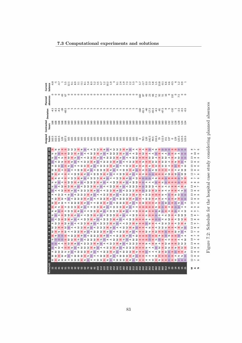
7.3 Computational experiments and solutions!"#$%&'(
))
*)
+)
,)
-)
)*
**
+*
,*
-*
.*
/*
0*
1*
)2*
))*
)**
)+*
),*
)-*
).*
)/*
)0*
)1*
*2*
*)*
***
*+*
*,*
*-*
*.*
*/*
*0*
*1*
+2*
+)*
)+
*+
),
*,
)-
*-
3 4 !
)*
+,
-.
/0
1)2
))
)*
)+
),
)-
).
)/
)0
)1
*2
*)
**
*+
*,
*-
*.
*/
*0
!!
"#
#$
%!
!"
#$
$%
!"
"#
$$
%!
!"
#$
$%
%!
!"
##
$%
!!
"#
$$
%!
""
#$
$%
!!
"#
$$
$%
!!
"#
#$
%!
!"
#$
$%
!"
"#
$$
%!
!"
#$
!!
!"
"#
#%
%%
%%
%%
!!
!!
!"
""
"#
$$
%%
$$
$%
%%
%!
!!
!!
""
""
"%
%%
%%
%%
%%
%%
"#
$%
!!
""
#$
%!
!!
"#
$%
!!
""
#$
%!
!!
!"
#$
%!
!"
"#
$%
!!
!"
#$
%!
!"
"#
$%
!!
!!
"#
$%
!!
""
#$
%!
!!
"#
$%
!!
""
#$
%!
!!
!"
#$
%!
!"
"#
$%
!!
!"
#$
%!
!"
"#
$%
%!
!!
"#
$%
!!
""
#$
%!
!!
"#
$%
!!
""
#$
$%
!!
!"
#$
%!
!"
"#
$%
!!
!"
#$
%!
!"
"#
#$
%!
!!
"#
$%
!!
""
#$
%!
!!
"#
$%
!!
""
"#
$%
!!
!"
#$
%!
!"
"#
$%
!!
!"
#$
%!
!"
""
#$
%!
!!
"#
$%
!!
""
#$
%!
!!
"#
$%
!!
!"
"#
$%
!!
!"
#$
%!
!"
"#
$%
!!
!"
#$
%!
!!
""
#$
%!
!!
"#
$%
!!
""
#$
%!
!!
"#
$%
%!
!"
"#
$%
!!
!"
#$
%!
!"
"#
$%
!!
!"
#$
$%
!!
""
#$
%!
!!
"#
$%
!!
""
#$
%!
!!
"#
#$
%!
!"
"#
$%
!!
!"
#$
%!
!"
"#
$%
!!
!"
"#
$%
!!
""
#$
%!
!!
"#
$%
!!
""
#$
%!
!!
!"
#$
%!
!"
"#
$%
!!
!"
#$
%!
!"
"#
$%
!!
!!
"#
$%
!!
""
#$
%!
!!
"#
$%
!!
""
#$
%!
!!
!"
#$
%!
!"
"#
$%
!!
!"
#$
%!
!"
"#
$%
%!
!!
"#
$%
!!
""
#$
%!
!!
"#
$%
!!
""
#$
$%
!!
!"
#$
%!
!"
"#
$%
!!
!"
#$
%!
!"
"#
#$
%!
!!
"#
$%
!!
""
#$
%!
!!
"#
$%
!!
""
"#
$%
!!
!"
#$
%!
!"
"#
$%
!!
!"
#$
%!
!"
%%
%%
%%
%%
%%
%%
%%
%%
%%
%%
%%
%%
%%
%%
%%
%%
%%
%%
%%
%%
%%
!"
"#
##
#$
$$
$%
!"
""
#$
$%
%!
"#
$$
$%
%!
!!
!"
#%
%%
%%
%%
""
""
"#
#$
$$
$%
%%
%!
!!
!"
##
#$
%!
"#
!"
""
%%
%%
%%
%%
%%
%%
%%
!"
"#
$%
!!
""
%!
"#
$$
%!
""
##
#$
$$
%!
"#
$%
!!
!"
#$
$%
!!
"#
$%
!"
#$
$%
%%
%%
%%
%%
%%
%%
%%
%%
%%
%%
%%
!!
""
##
#$
$$
$$
%%
%!
!!
"#
%%
!!
!"
##
$$
$$
%%
!"
""
"#
#$
%!
!!
"#
##
#$
$$
$%
%!
!!
""
##
#$
$%
%!
""
""
##
%%
%%
%%
%%
%%
%%
%%
%%
%%
%%
%%
%%
%%
%%
!"
#$
%%
%!
""
""
##
#$
$%
%%
%!
"#
$$
$%
#$
%%
!"
#$
%!
!!
"#
$%
!"
"#
##
$%
%!
"#
#$
%!
!"
"#
$%
!!
""
##
#$
%%
!!
!"
##
##
##
$%
!!
""
#$
%!
!"
"#
##
$%
%!
!!
"#
##
&'
&'
&(
&'
&(
&)
*&'
&'
&(
&'
&(
+*
&'
&'
&(
&'
&(
++
&'
&'
&(
&'
&(
+*
,*
**
*,
,,
*+
**
++
,*
+*
**
,,
**
**
&)
,
--
--
--
--
-,
-,
,-
--
--
,-
--
--
--
--
4$$56'%7
89':#;<:%7
=>;''%7?
8"##%':
@9"#$
@9"#$
;A$%'<%$
A;>;'<%
&-(./
&-*
01./
)0-.*
&-(./
&-*
01./
)0/
&-(./
&-*
01./
)01.,
&'+
&-*
0(+
1(
&
&),./
&-*
0-)./
-,
/./
&-/
&-)
/)
&'.&
&-/
&-)
/)
+.&
&-/
&-)
/)
*.+
&-/
&-)
/)
(.&
&-/
&-)
/)
0(.&
&-/
&-)
/)
*.&
&-/
&-)
/)
/.1
&-/
&-)
/)
*.(
&-/
&-)
/)
/.'
&-/
&-)
/)
(./
&-/
&-)
/)
1.,
&-/
&-)
/)
&.'
&-/
&-)
/)
&).'
&-/
&-)
/)
&.+
&-/
&-)
/)
(
&-/
&-)
/)
+.&
&-/
&-)
/)
'.1
&-/
&-)
/)
&.+
&-/
&-)
/)
,.(
&-/
&-)
/)
'.'
&-/
&-)
/)
/.(
&-/
&-)
/)
,
)&-)
0&-)
&-)
/.,
,*./
&-)
0*&./
*,
0(.,
&')
&-)
01)
1(
).(
&1'./
&-)
0&,./
'(
'.(
+1./
&-)
0-/./
--
/.*
&//./
&-)
01./
,./
&./
,+
&-)
0*&
+'
&(.*
&&'./
&-)
01,./
/&
0).&
&/&
&-)
0+&-
-.-
&(,
&('
/)
1.-
)&('
0&('
&('
0)./
&'+
&'*
&)
-
&'/./
&'*
0'./
,./
&.'
&'(./
&'1
0)./
)).+
&'(./
&'1
0)./
)&
(%B5;:59'
Fig
ure
7.2:
Sche
dule
for
the
hosp
ital
case
stud
yco
nsid
erin
gpl
anne
dab
senc
es
83
Chapter 7. Application of the general model to a hospital
these deviations (translated by the objective function). In order to get an
optimal solution in a reasonable time, a lower bound to the objective func-
tion was imposed. After testing several values, the best compromise was
found for the solution of Fig. 7.2, with an objective function of 200.
The limits on the daily shift requirements dMaxDsd and dMinDsd have
also a significant influence on the model’s performance. The closer to real
data these parameters are set, the tighter the model gets and the longer
it takes to reach a solution. In our approach, only the dMinDsd real data
was imposed. The limits on dMaxDsd had to be relaxed in order to get a
solution in a reasonable amount of time. Looking again into the solution of
Fig. 7.2, the information on the daily assigned hours can be checked in the
rows below the schedule, for each one of the working shifts. A comparison of
these figures with the initial demand requirements proves that the minimum
daily requirements are satisfied, whereas the maximum limits are violated
in 6 different days: one extra morning shift on day 6, one extra afternoon
shift on days 10, 13, 14 and 17, and two afternoon shifts in excess on day 27.
This drawback does not seem very representative when we look at the real
solution, where the number of similar violations is much higher, reaching 23
situations, mostly affecting the afternoon and night shifts. Nevertheless, we
do not have enough information to evaluate the impact of these violations
in the real setting.
7.4 Conclusions
This chapter described the application of the general IP model to the prob-
lem of nurse scheduling in a Portuguese hospital (Antunes and Moz (2011)).
This problem differs from the others already described in the previous two
chapters (Chapters 5 and 6) in two main features: the workforce compo-
sition and the objective. The workforce is now composed of 5 groups of
84

7.4 Conclusions
nurses, which are grouped according to their contract types. The objec-
tive is to minimize the gap between assigned and contracted hours. The
cyclic approach introduced in Chapter 5 was adopted in order to ensure a
balanced solution within each group of nurses. Demand constraints (Eqs.
4.5, 7.2 and 7.3) were adapted in order to consider minimum and maximum
daily requirements for each shift. Equations (5.3), (5.4) and (5.5) to each
contract type (index k) made it possible to impose different limits on the
number of consecutive working/rest days to each group of nurses. In this
problem, it was more reasonable to allow the groups with less contracted
hours to have more days-off assignments than the others. A new sequence
of shifts and days-off that met the preferences of the nurses was imposed, by
simply defining a new vector of indices n(s′). Although it was not considered
in this problem, we could define different sequence patterns to each group
of nurses by simply indexing the sequence constraints (Eqs. 5.6) to each
type of contract. This example illustrates the flexibility and potential of the
proposed formulation. Experiments focused on finding a trade-off between
the value of the optimal solution and the computational time. In order to
compare our solution with the one proposed by Antunes and Moz (2011)
and the real solution manually developed by the head nurse of the hospi-
tal, we adjusted the model to consider the absences planned for the present
month. An optimal solution was built in 38 minutes, considerably more
than the 0.38 seconds taken by the optimal solution proposed by Antunes
and Moz (2011), which was specifically tailored to this problem, but much
less than the 8 hours the head nurse needed to develop it by hand. Results
are encouraging, demonstrating that our formulation can also accommodate
restrictions on planned absences, such as holiday or training.
85

Chapter 7. Application of the general model to a hospital
86
Chapter 8
Benchmark instances
In order to evaluate the flexibility and wide scope of the developed formula-
tion and to compare results with other approaches, experiments were carried
out on a collection of 20 rotating workforce scheduling problems available
in http://www.dbai.tuwien.ac.at/staff/musliu/benchmarks and presented in
Musliu (2006). This chapter describes the application of the general model
introduced in Chapter 4 to those benchmark problems. Section 8.1 presents
the features of the problems. Next, the adjustments that were made to the
general formulation are explained in Section 8.2, giving special attention to
the sequence constraints adaptation. Section 8.3 shows the computational
results and a comparison with other methods. Solutions are discussed in
Section 8.4, followed by some concluding remarks that end the chapter.
8.1 Problem description
In these instances, the number of employees vary from 7 to 163. The num-
ber of standard shifts is either 2 (day and afternoon) or 3 (day, afternoon
and night). The length of working and days-off blocks is now limited by a
minimum and a maximum number of consecutive days, as well as the length
of each sequence of days assigned to the same shift. In the previous case
87
Chapter 8. Benchmark instances
studies only this last situation is considered. The main difference from these
problems to the previous ones is the existence of a set of forbidden shift se-
quences, instead of a predefined sequence to follow. The forbidden sequences
that are imposed are of two types: (N-D, N-A and A-D) or (N-B-N, A-B-D,
N-B-A and N-B-D). Naturally, the second type is considered only if a sin-
gle day-off is allowed. Otherwise, only the first type is taken into account.
Problems have either both types of forbidden sequences or only type 1.
8.2 Mathematical model
The formulation used to solve these problems followed the adaptations made
for the glass unit problem (Chapter 5). We refer to Section 5.2 for further
details. This section is therefore focused on new adjustments: limits on the
length of working and days-off blocks and, especially, a new perspective in
the sequence constraints. Following the same reasoning used in the previous
case studies, it is possible to define allowable sequences for each given type
of forbidden sequences.
Consider the 3 working shifts {D,A,N} as {1, 2, 3} and the 3 non-working
shifts as {4, 5, 6}. Unlike the previous case studies, this is not the only
sequence allowed. For the first type of forbidden sequences: N-D, N-A and
A-D, the allowed sequences can be represented as shown in Table 8.1. n(s′)
is the extended shift that can follow the extended shift s′ in a given sequence.
From Table 8.1, it is possible to realize that only the shifts that follow the
shifts 2 and 3 must be constrained. All the remaining shifts can be followed
by any of the other shifts, inclusive by themselves. The sequence constraints
in the general mathematical model are therefore replaced by the following
constraints:
88

8.2 Mathematical model
s′ 1 2 3 4 5 6
n(s′)
4 5 6 1 1 1
2 3 2 2 2
3 3 3 3
5 5 4 4
6 6 6 5
Table 8.1: First type of allowable sequences
∀td xt2d − xt2(d+1) − xt5(d+1) − xt3(d+1) ≤ 0 (8.1)
∀td xt3d − xt3(d+1) − xt6(d+1) ≤ 0 (8.2)
Considering now both types of forbidden sequences: N-D, N-A, A-D, N-B-N,
A-B-D, N-B-A and N-B-D, the allowed sequences are represented in Table
8.2.
s′ 1 2 3 4 5 6
n(s′)
4 6 4 1 1 2
2 3 2 2 3
3 3 3 4
5 5 4 5
6 6 6
Table 8.2: Allowable sequences
Note that, in this case, shift 3 (N) can only be followed by another shift 3 or
by a minimum of two consecutive days-off (B). To simplify the model and
in order to satisfy this limitation, shift 4 is now defined as the non-working
89

Chapter 8. Benchmark instances
shift that follows shift 3 and, in the model’s parameterization, the minimum
number of consecutive days (minD′s) indexed to shift 4 is set to 2. The
sequence constraints in the general mathematical model are now restricted
to the constraints on shifts 2, 3 and 6, defined as follows:
∀td xt2d − xt2(d+1) − xt6(d+1) − xt3(d+1) ≤ 0 (8.3)
∀td xt3d − xt3(d+1) − xt4(d+1) ≤ 0 (8.4)
∀td xt6d − xt6(d+1) − xt2(d+1) − xt3(d+1) − xt4(d+1) ≤ 0 (8.5)
For the problems with only two shifts {1,2}, the only forbidden sequence is
A-D, and so the allowed sequences are represented in Table 8.3.
s′ 1 2 3 4
n(s′)
2 4 2 1
3 3 4 3
4 1 2
Table 8.3: Allowable sequences for nS=2
The sequence constraints in the general mathematical model are replaced
by the following constraints:
∀td xt2d − xt2(d+1) − xt4(d+1) − xt3(d+1) ≤ 0 (8.6)
8.3 Computational experiments
Like in the previous case studies, this model was also coded in OPL Studio
version 6.3 and solved using the CPLEX 12.1.0 solver on a server machine
90

8.3 Computational experiments
powered by 2 Intel R© Xeon R© processors of 2,4 GHz and 1,39 GHz, and
with 2 GB RAM. Tests were performed for the 20 instances and results are
shown in Table 8.4. The offset considered for all the examples is 7 days, so
the planning periods are defined by 7× nT . The optimization model found
the optimal solution for 12 problems, with the number of employees varying
from 7 to 29. For the remaining problems, signed with “-”, the optimization
model did not reach any feasible solution within 20000 seconds of running
time. This happened for all the instances with more than 27 employees. The
model is able to reach an optimal solution for problem 16, for example, while
for problem 7 it does not find any feasible solution. Although both problems
have the same number of employees, 29, the shift daily demand, the limits on
the length of shift sequences, working-day and days-off blocks differ from one
problem to another. It is evident that the combination of these parameters
has a decisive influence on the complexity of each problem and consequently
on the model’s performance. In Musliu (2006), the best resolution times
for these instances are achieved by a tabu search based heuristic (MC-T).
In the same work, Musliu compares the resolution times of MC-T with the
ones achieved by a commercial software, First Class Scheduler (FCS). The
resolution times achieved by Musliu with FCS are also reported in the last
column of Table 8.4, where “-” signs the problems to which FCS did not find
any solution within 1000 seconds of running time. As expected, comparison
of resolution times shows that the heuristic based method outperforms the
optimization approach in all instances. Nevertheless, when comparing the
resolution times obtained by the IP model and FCS, we can conclude that
the former has better times for 7 of these instances than the latter.
91

Chapter 8. Benchmark instances
8.4 Solutions
The comparison of the values of the objective functions proves that the
solutions obtained by the MC-T method are all optimal (have the same
value), in spite of the different pattern composition of the schedules. As an
example, Fig. 8.1 and Fig. 8.2 show the solutions obtained for Ex. 6 with
our IP optimization model and with MC-T respectively. The optimal value
of the objective function is 12 for both solutions.
!" # $ % & ' ( ) * + #, ## #$ #% #& #' #( #) #* #+ $, $# $$ $% $& $' $( $) $* $+ %, %# %$ %% %& %' %( %) %* %+ &, &# &$ &% && &' &( &) &* &+ ! " #
-# D D D D D D -- A A N N N -- -- D D D D D D -- A A A A A A -- -- -- A A A A N N N -- -- -- -- N N N N N N -- -- #$ #$ #$
-$ N N N N N -- -- D D D D D D -- A A N N N -- -- D D D D D D -- A A A A A A -- -- -- A A A A N N N -- -- -- -- N #$ #$ #$
-% N N -- -- -- -- N N N N N N -- -- D D D D D D -- A A N N N -- -- D D D D D D -- A A A A A A -- -- -- A A A A N #$ #$ #$
-& -- -- A A A A N N N -- -- -- -- N N N N N N -- -- D D D D D D -- A A N N N -- -- D D D D D D -- A A A A A A -- #$ #$ #$
-' A A A A A A -- -- -- A A A A N N N -- -- -- -- N N N N N N -- -- D D D D D D -- A A N N N -- -- D D D D D D -- #$ #$ #$
-( D D D D D D -- A A A A A A -- -- -- A A A A N N N -- -- -- -- N N N N N N -- -- D D D D D D -- A A N N N -- -- #$ #$ #$
-) A A N N N -- -- D D D D D D -- A A A A A A -- -- -- A A A A N N N -- -- -- -- N N N N N N -- -- D D D D D D -- #$ #$ #$
! $ $ $ $ $ $ , $ $ $ $ $ $ , $ $ $ $ $ $ , $ $ $ $ $ $ , $ $ $ $ $ $ , $ $ $ $ $ $ , $ $ $ $ $ $ ,
" $ $ $ $ $ $ , $ $ $ $ $ $ , $ $ $ $ $ $ , $ $ $ $ $ $ , $ $ $ $ $ $ , $ $ $ $ $ $ , $ $ $ $ $ $ ,
# $ $ $ $ $ , $ $ $ $ $ $ , $ $ $ $ $ $ , $ $ $ $ $ $ , $ $ $ $ $ $ , $ $ $ $ $ $ , $ $ $ $ $ $ , $
Figure 8.1: IP solution for Ex6
!" # $ % & ' ( ) * + #, ## #$ #% #& #' #( #) #* #+ $, $# $$ $% $& $' $( $) $* $+ %, %# %$ %% %& %' %( %) %* %+ &, &# &$ &% && &' &( &) &* &+ ! " #
-# D D D N N N N N N N N N N D D D D D D A A A A A A A A A N N D D D A A A #$ #$ #$
-$ D D D A A A D D D N N N N N N N N N N D D D D D D A A A A A A A A A N N #$ #$ #$
-% A A A N N D D D A A A D D D N N N N N N N N N N D D D D D D A A A A A A #$ #$ #$
-& A A A A A A A A A N N D D D A A A D D D N N N N N N N N N N D D D D D D #$ #$ #$
-' D D D D D D A A A A A A A A A N N D D D A A A D D D N N N N N N N N N N #$ #$ #$
-( N N N N N D D D D D D A A A A A A A A A N N D D D A A A D D D N N N N N #$ #$ #$
-) N N N N N N N N N D D D D D D A A A A A A A A A N N D D D A A A D D D N #$ #$ #$
! $ $ $ $ $ $ , $ $ $ $ $ $ , $ $ $ $ $ $ , $ $ $ $ $ $ , $ $ $ $ $ $ , $ $ $ $ $ $ , $ $ $ $ $ $ ,
" $ $ $ $ $ $ , $ $ $ $ $ $ , $ $ $ $ $ $ , $ $ $ $ $ $ , $ $ $ $ $ $ , $ $ $ $ $ $ , $ $ $ $ $ $ ,
# $ $ $ $ $ , $ $ $ $ $ $ , $ $ $ $ $ $ , $ $ $ $ $ $ , $ $ $ $ $ $ , $ $ $ $ $ $ , $ $ $ $ $ $ , $
Figure 8.2: Benchmark solution for Ex6
8.5 Conclusions
In this chapter a set of 20 benchmark instances was used to demonstrate
the consistency and wide scope application of the general model proposed
in Chapter 4. These instances vary in size, shift daily requirements and also
in the types of shift sequences. The general model was adjusted in order
to accommodate a new perspective on the sequence constraints. Instead of
having a single allowable sequence of shifts and days-off, the new problems
imposed a set of forbidden sequences. This means allowing for multiple
feasible sequences. The adaptation of the sequence constraints (Eqs. 4.9)
92

8.5 Conclusions
was explained in detail in Section 8.2. Once more, the versatility of the
proposed formulation is evident from this application. The optimization
model found the optimal solution for 12 problems, some of them of very
large dimension, which corresponds to a success rate of 60% of the total
number of problems considered. The solutions were compared with the ones
achieved by Musliu (2006). Although the exact matching of the objective
function values, the schedules developed by both methods (IP and MC-T)
differ in the patterns of shifts and days-off assigned. An example for Ex.6
is shown in Section 8.4.
93

Chapter 8. Benchmark instances
Time(sec.)
Ex. nD nT nS IP MC-T FCS
1 63 9 3 7.94 0.07 0.90
2 63 9 3 2.90 0.07 0.40
3 119 17 3 907.40 0.42 1.90
4 91 13 3 1.59 0.11 1.70
5 77 11 3 2.47 0.43 3.50
6 49 7 3 1.23 0.08 2.00
7 203 29 3 - 52.79 16.10
8 112 16 3 7.60 0.74 124.00
9 329 47 3 - 15.96 -
10 189 27 3 - 0.60 9.50
11 210 30 3 - 13.15 367.00
12 140 20 2 310.00 1.17 -
13 49 7 3 255.95 0.87 -
14 91 13 3 73.14 0.76 0.54
15 448 64 3 - 159.04 -
16 203 29 3 1923.00 0.54 2.44
17 231 33 2 29.64 2.16 -
18 371 53 3 - 6.83 2.57
19 840 120 3 - 75.83 -
20 1141 163 3 - 71.38 -
Table 8.4: Computational times for the benchmarking instances using theIP model, MC-T and FCS
94
Chapter 9
Heuristic approach
An optimization approach is typically limited in terms of performance for
real-life large dimension problems. The challenge of developing a heuris-
tic procedure naturally arose as a means of systematically overcoming that
handicap and to compare results. In this chapter we propose a construc-
tive heuristic to solve the problem of the glass unit addressed in Chapter 5.
Section 9.1 describes the heuristic procedure, explaining the initial assump-
tions and the developed algorithms. Computational results for the glass unit
problem are shown in Section 9.2 and a comparison of the performance of
both approaches, heuristic and optimization, is carried out. In order to an-
alyze the consistency of the heuristic, a set of computer generated instances
was also used, varying in size with the number of teams and the number
of shifts. The solutions generated for the glass unit problem are presented
in Section 9.2. Section 9.3 draws some conclusions and reflexions for future
extensions of this work.
95

Chapter 9. Heuristic approach
9.1 Heuristic
9.1.1 Initial assumptions
From our previous experience with the optimization model, described in
Chapter 5, we realized that a key issue that guarantees the existence of fea-
sible solutions is the availability of a sufficient number of breaks, to allow
for an adequate sequence of working days and days-off for each team. This
break availability condition is on the basis of the proposed heuristic. When
the condition is valid, for a set of input parameters, the heuristic defines
a feasible schedule for the first team, which will be afterwards replicated
for the remaining teams, with a time lag or offset days in between. In the
development of the first team’s schedule, working-day blocks are assigned
following the sequence of the shifts in which the teams must work. The
length of the working blocks is limited by the minimum and maximum num-
bers of allowable consecutive working days. It may occur, therefore, that all
working blocks have the same length, i.e. the same number of consecutive
days, or that blocks have different lengths. Between each two consecutive
working blocks, i.e., between each change of working shifts, there must be
at least one break day. The heuristic assures that blocks of working days
plus breaks have always the same length. Therefore, in the case of a sched-
ule with working-day blocks with different lengths, more than one break is
assigned after the working blocks with shorter lengths, in order to have a
block of working days plus breaks with the same length as the block with the
maximum length plus one break. The heuristic tests different combinations
of working blocks until a feasible solution is reached. These procedures are
next explained in detail.
96

9.1 Heuristic
9.1.2 Algorithm 1 - checkAvailableBreaks
The first step of the heuristic is the verification of the available breaks con-
dition, described in Algorithm 1 - checkAvailableBreaks, where:
nD is the number of days in the planning period;
nT is the number of teams;
nS is the number of working shifts;
minD is the minimum required number of consecutive working days;
maxD is the maximum allowed number of consecutive working days;
wd is the number of working days of the planning period to be assigned
to each team, for each shift;
nblocks is the number of blocks of working days, for each team and for each
shift;
maxBlock is the block of working days with the maximum length to be consid-
ered;
Ftot is the total number of available breaks in the planning period, for each
team;
Fmin is the minimum number of required breaks in the planning period, for
each team, considering the required number of working-day blocks.
The algorithm first calculates the values for Ftot and wd. If, in each day,
there are 3 shifts to be assigned to exactly 3 teams, the remaining 2 teams are
necessarily assigned to breaks. So, 2 breaks are available in each day. These
2 breaks multiplied by the number of days in the planning period (nD) and
divided by the number of teams (nT ) result in the total number of available
97

Chapter 9. Heuristic approach
Algorithm 1 checkAvailableBreaks
Ftot ← nD ∗ (nT − nS)/nTwd ← (nD − Ftot)/nS
for i = 0→ (minD + i) doif wd is a multiple of (minD + i) then
nblocks ← wd/(minD + i)Fmin ← nblocks ∗ nSif Fmin ≤ Ftot then
solutionExistsmaxBlock ← (minD + i)equalBlocksExit
end ifend if
end fortestBlocksCombination()
if solutionExists thenExit
elsenoFeasibleSolutionAssuredExit
end if
breaks per team, Ftot. This figure represents the maximum number of breaks
the procedure has available to assign to each team, and must be enough to
ensure the mandatory minimum number of breaks to assign between shift
changes. Taking Ftot out of nD and dividing it by the number of shifts (nS)
we get the number of working days, in each shift, to assign to each team,
wd. Figures 9.1, 9.2 and 9.3 illustrate the reasoning of these calculations
for nD = 20 days, breaks are represented by the blank cells. Algorithm 1
proceeds by checking the possibility of assigning only working blocks with
equal length: (minD + i). Looking into the same example of nD = 20
days, with minD = 2 days and maxD = 4 days, the number of days in
each of the working blocks is achieved for i = 0, thus wd/2 = 2. When
that is not feasible, the function testBlocksCombination() is called and
98

9.1 Heuristic
combinations of working blocks with different lengths are evaluated. This
is the case illustrated in Fig. 9.4, for a planning period of 25 days. In this
scenario, wd = 5 days, which is not divisible for any minD + i, for any i.
Therefore, a combination of blocks of minD and minD + 1 days, 2 days
and 3 days respectively, is used. If no combination of blocks satisfies the
condition Fmin ≤ Ftot, then the problem may not have a feasible solution.
Consequently, the following statement can be made:
If the input parameters selected verify the condition: Fmin ≤
Ftot, then it has a feasible solution. Otherwise, it may have or
not a feasible solution.
This condition is thus sufficient but not necessary.
Teams/Days 1 2 3 4 5 6 7 8 9 10 11 12 13 14 15 16 17 18 19 20
T1 !" !" !! #" #" !! $" $" !! !! !" !" !! #" #" !! $" $" !! !!
T2 !! !! !" !" !! #" #" !! $" $" !! !! !" !" !! #" #" !! $" $"
T3 $" $" !! !! !" !" !! #" #" !! $" $" !! !! !" !" !! #" #" !!
T4 #" !! $" $" !! !! !" !" !! #" #" !! $" $" !! !! !" !" !! #"
T5 !! #" #" !! $" $" !! !! !" !" !! #" #" !! $" $" !! !! !" !"
Figure 9.1: Example: calculation of the number of available breaks/day.
Teams/Days 1 2 3 4 5 6 7 8 9 10 11 12 13 14 15 16 17 18 19 20
T1 !" !" !! #" #" !! $" $" !! !! !" !" !! #" #" !! $" $" !! !!
T2 !! !! !" !" !! #" #" !! $" $" !! !! !" !" !! #" #" !! $" $"
T3 $" $" !! !! !" !" !! #" #" !! $" $" !! !! !" !" !! #" #" !!
T4 #" !! $" $" !! !! !" !" !! #" #" !! $" $" !! !! !" !" !! #"
T5 !! #" #" !! $" $" !! !! !" !" !! #" #" !! $" $" !! !! !" !"
Figure 9.2: Example: calculation of the number of available breaks/team.
99
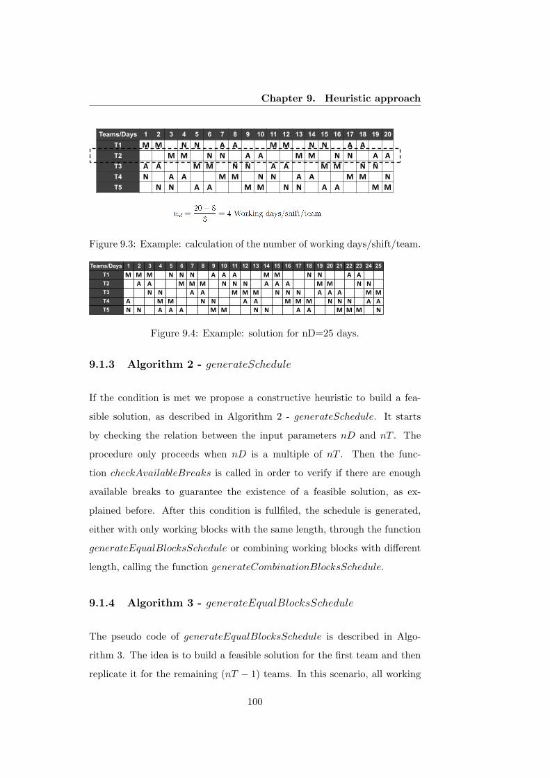
Chapter 9. Heuristic approach
Teams/Days 1 2 3 4 5 6 7 8 9 10 11 12 13 14 15 16 17 18 19 20
T1 !" !" !! #" #" !! $" $" !! !! !" !" !! #" #" !! $" $" !! !!
T2 !! !! !" !" !! #" #" !! $" $" !! !! !" !" !! #" #" !! $" $"
T3 $" $" !! !! !" !" !! #" #" !! $" $" !! !! !" !" !! #" #" !!
T4 #" !! $" $" !! !! !" !" !! #" #" !! $" $" !! !! !" !" !! #"
T5 !! #" #" !! $" $" !! !! !" !" !! #" #" !! $" $" !! !! !" !"
Figure 9.3: Example: calculation of the number of working days/shift/team.
Teams/Days 1 2 3 4 5 6 7 8 9 10 11 12 13 14 15 16 17 18 19 20 21 22 23 24 25
T1 ! ! ! " " " # # # ! ! " " # #
T2 # # ! ! ! " " " # # # ! ! " "
T3 " " # # ! ! ! " " " # # # ! !
T4 # ! ! " " # # ! ! ! " " " # #
T5 " " # # # ! ! " " # # ! ! ! "
Figure 9.4: Example: solution for nD=25 days.
9.1.3 Algorithm 2 - generateSchedule
If the condition is met we propose a constructive heuristic to build a fea-
sible solution, as described in Algorithm 2 - generateSchedule. It starts
by checking the relation between the input parameters nD and nT . The
procedure only proceeds when nD is a multiple of nT . Then the func-
tion checkAvailableBreaks is called in order to verify if there are enough
available breaks to guarantee the existence of a feasible solution, as ex-
plained before. After this condition is fullfiled, the schedule is generated,
either with only working blocks with the same length, through the function
generateEqualBlocksSchedule or combining working blocks with different
length, calling the function generateCombinationBlocksSchedule.
9.1.4 Algorithm 3 - generateEqualBlocksSchedule
The pseudo code of generateEqualBlocksSchedule is described in Algo-
rithm 3. The idea is to build a feasible solution for the first team and then
replicate it for the remaining (nT − 1) teams. In this scenario, all working
100

9.1 Heuristic
Algorithm 2 generateSchedule
if nD is not a multiple of nT thenMsg: ”Change input parameters”
end ifcheckAvailableBreaks
if solutionExists then initializeScheduleif equalBlocks thengenerateEqualBlocksSchedule
elsegenerateCombinationBlocksSchedule
end ifelse if noFeasibleSolutionAssured then
Msg: ”Fmin > Ftot, the problem may not have a feasible solution!”end if
blocks have the same length of maxBlock days and are separated by one
break. The procedure begins by assigning the first block of the first working
shift to all teams, with a time lag, δD, equal to minD days between them,
if maxBlock ≤ minD or, otherwise, equal to nD/nT days. It proceeds by
assigning the first blocks of the remaining shifts to the first team, separated
by a break. In order to satisfy the shift daily demand, which forces each
working shift to be assigned to only one team in each day of the planning
period, the second sub-period can only begin when the first shift is available
again, and for maxBlock consecutive days. This means that the second
working block of the first shift can only be assigned to team 1 in a slot with,
at least, maxBlock consecutive days where there isn’t any team assigned
to that shift. The first sub-period is then replicated for the first team until
the whole planning period is fulfilled, resulting in the schedule for the first
team. This schedule is replicated for all the remaining (nT − 1) teams, with
a time lag of δD days between them.
101
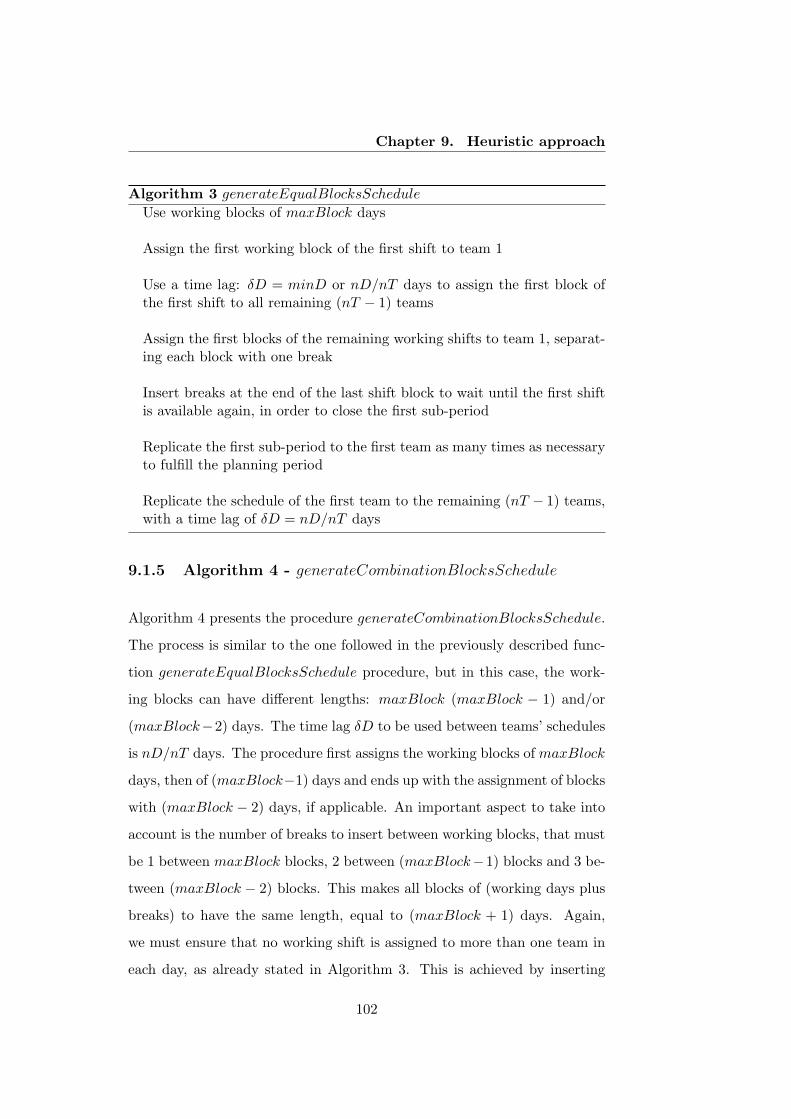
Chapter 9. Heuristic approach
Algorithm 3 generateEqualBlocksSchedule
Use working blocks of maxBlock days
Assign the first working block of the first shift to team 1
Use a time lag: δD = minD or nD/nT days to assign the first block ofthe first shift to all remaining (nT − 1) teams
Assign the first blocks of the remaining working shifts to team 1, separat-ing each block with one break
Insert breaks at the end of the last shift block to wait until the first shiftis available again, in order to close the first sub-period
Replicate the first sub-period to the first team as many times as necessaryto fulfill the planning period
Replicate the schedule of the first team to the remaining (nT − 1) teams,with a time lag of δD = nD/nT days
9.1.5 Algorithm 4 - generateCombinationBlocksSchedule
Algorithm 4 presents the procedure generateCombinationBlocksSchedule.
The process is similar to the one followed in the previously described func-
tion generateEqualBlocksSchedule procedure, but in this case, the work-
ing blocks can have different lengths: maxBlock (maxBlock − 1) and/or
(maxBlock−2) days. The time lag δD to be used between teams’ schedules
is nD/nT days. The procedure first assigns the working blocks of maxBlock
days, then of (maxBlock−1) days and ends up with the assignment of blocks
with (maxBlock − 2) days, if applicable. An important aspect to take into
account is the number of breaks to insert between working blocks, that must
be 1 between maxBlock blocks, 2 between (maxBlock−1) blocks and 3 be-
tween (maxBlock − 2) blocks. This makes all blocks of (working days plus
breaks) to have the same length, equal to (maxBlock + 1) days. Again,
we must ensure that no working shift is assigned to more than one team in
each day, as already stated in Algorithm 3. This is achieved by inserting
102

9.2 Computational experiments and solutions
Algorithm 4 generateCombinationBlocksSchedule
Use a combination of working blocks of maxBlock, (maxBlock−1) and/or(maxBlock − 2) days, if applicable
for i = 0→ 2 do
Assign the first (maxBlock− i) working block of the first shift to team1
Use a time lag: δD = nD/nT to assign the first (maxBlock− i) blockof the first shift to all remaining (nT − 1) teams
Assign the first (maxBlock− i) block of the remaining working shiftsto team 1, separating each block with (i+ 1) breaks
Insert breaks at the end of the last shift block to wait until the firstshift is available again, in order to close the first sub-period
end for
Replicate the first sub-period to the first team as many times as necessaryto fulfill the planning period
Replicate the schedule of the first team to the remaining (nT − 1) teams,with a time lag of δD = nD/nT days
breaks at the end of the last working block of the first sub-period until the
first shift is available again for the second sub-period assignment. The first
sub-period is then replicated to the first team as many times as necessary
in order to complete the whole planning period, resulting in the schedule
for the first team. This schedule is replicated to all the remaining (nT − 1)
teams, with a time lag of δD days between them.
9.2 Computational experiments and solutions
The heuristic was coded using VBA for Excel 2011 and ran on a server
machine powered by 2 Intel R© Xeon R© processors of 2,4 GHz and 1,39 GHz,
103
Chapter 9. Heuristic approach
and with 2 GB RAM. Tests were made for both 4 and 5 teams of employees
and planning periods ranging up to 365 days. Several combinations of input
parameters: number of days in the planning period (nD) and time lag,
or offset days (δD), were considered. Feasible solutions were consistently
found, except for periods of 125 and 275 days, where the heuristic didn’t find
any combination of working-day blocks to build a feasible solution. When
comparing with the solutions generated by the IP model, it is possible to
conclude that the heuristic always reaches the optimal solution, in what
concerns to the value of the objective function. However, the composition
of the schedule is not the same in the solutions obtained by both methods.
This can be explained by the fact that the IP model does not impose the
same schedule structure that is naturally imposed by the heuristic procedure.
Although the schedules are not exactly equal, the quality of the solutions
in terms of work balance is not compromised since all teams work the same
number of days, in each shift, along the planning horizon. Two examples
are shown in Figs. 9.1 - 9.3 and 9.4, for planning periods of 20 and 25 days
respectively.
Table 9.1 presents computational times for a set of different combinations
of nD and δD, which verify the integer relationship between them.
The heuristic reaches a feasible solution in less than 0.5 seconds for planning
periods up to 180 days, and in less than a minute for 330 and 365 days,
while the IP model takes longer times as the length of the planning period
increases. For 330 and 365 days the execution of the IP model was stopped
after 60000 seconds, without finding any feasible solution. A comparison
between the computational times taken by both methods reveals that the
heuristic consistently outperforms the optimization model.
The definition of the planning period is not a very explored issue in the
literature, since it is closely related to demand forecast periods and it is
104
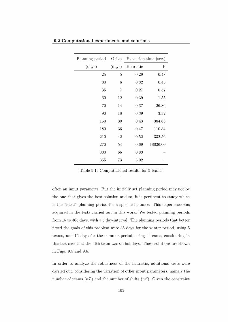
9.2 Computational experiments and solutions
Planning period Offset Execution time (sec.)
(days) (days) Heuristic IP
25 5 0.29 0.48
30 6 0.32 0.45
35 7 0.27 0.57
60 12 0.39 1.55
70 14 0.37 26.86
90 18 0.39 3.32
150 30 0.43 384.63
180 36 0.47 110.84
210 42 0.52 332.56
270 54 0.69 18026.00
330 66 0.83 –
365 73 3.92 –
Table 9.1: Computational results for 5 teams.
often an input parameter. But the initially set planning period may not be
the one that gives the best solution and so, it is pertinent to study which
is the “ideal” planning period for a specific instance. This experience was
acquired in the tests carried out in this work. We tested planning periods
from 15 to 365 days, with a 5 day-interval. The planning periods that better
fitted the goals of this problem were 35 days for the winter period, using 5
teams, and 16 days for the summer period, using 4 teams, considering in
this last case that the fifth team was on holidays. These solutions are shown
in Figs. 9.5 and 9.6.
In order to analyze the robustness of the heuristic, additional tests were
carried out, considering the variation of other input parameters, namely the
number of teams (nT ) and the number of shifts (nS). Given the constraint
105

Chapter 9. Heuristic approach
Teams/Days 1 2 3 4 5 6 7 8 9 10 11 12 13 14 15 16 17 18 19 20 21 22 23 24 25 26 27 28 29 30 31 32 33 34 35 ! " #
T1 ! ! ! ! # # # # " " " " ! ! ! # # # " " " ! ! ! $%
T2 " " " ! ! ! ! # # # # " " " " ! ! ! # # # ! ! ! $%
T3 # # # " " " ! ! ! ! # # # # " " " " ! ! ! ! ! ! $%
T4 ! ! ! # # # " " " ! ! ! ! # # # # " " " " ! ! ! $%
T5 # # " " " " ! ! ! # # # " " " ! ! ! ! # # ! ! ! $%
&'()*
Figure 9.5: Solution for nD=35 days.
Teams/Days 1 2 3 4 5 6 7 8 9 10 11 12 13 14 15 16 ! " #
T1 ! ! ! ! # # # # " " " " ! ! ! $%
T2 " " ! ! ! ! # # # # " " ! ! ! $%
T3 # " " " " ! ! ! ! # # # ! ! ! $%
T4 # # # # " " " " ! ! ! ! ! ! ! $%
&'()*
Figure 9.6: Solution for nD=16 days.
that imposes that, on each day, each working shift must only be assigned
to exactly one team, there is a ratio between nT and nS that must be kept
reasonable. It is not realistic to significantly increase the number of teams
without simultaneously increasing the number of shifts because, in that sit-
uation, there would be too many teams without any working shift assigned
on each day and the problem would become too simple and senseless. Table
9.2 presents the computational results achieved for the 48 instances, and
that were created having this reasoning in mind. The instances consider the
division of each 8-hour daily working shift (M, A and N) in several work
stations. In this scenario, nS refers to the number of work stations. Each
team of employees must cover all work stations, following the predefined
sequence of work shifts: M-N-A, and a break day between each shift change
must still be guaranteed. Whenever a team returns to the same work shift,
it moves on to the next work station. Figure 9.7 illustrates an example of
this process for 9 work stations, 3 for each work shift.
!"# $"# %"#&# &# &# !'# $'# %'#&# &# &# !(# $(# %(#&# &# &# !"# )))#
Figure 9.7: Example: sequence for 9 work stations (nS=9).
Following this reasoning, the values for nS were set considering always mul-
tiples of 3, up to 30. nT varies from 4 to 50 teams and nD from 16 up
106

9.2 Computational experiments and solutions
to 152 days. In terms of the ratio between nS and nT , tests were made
for nS/nT = 0.60, 0.70, 0.75 and 0.80. However, not all of these values can
be verified for all nS. For example, for nS = 3 it is not possible to have
nS/nT = 0.8, since 3/4 = 0.75 and it is not possible to have simultaneously
nS = 3 and nT = 3, since there must be breaks to interpose between the
working blocks. The closer the ratio nS/nT gets to 1, the tighter the prob-
lem becomes, as there are few breaks compared to the number of teams.
Again, it is possible to see the robustness and consistency of the heuristic
results, which fall below 5 seconds, even for a large number of teams. The IP
results, on the contrary, reveal an unsteady performance and, for instances
with more than 30 teams, it does not find any feasible solution at all, within
60000 seconds of running time.
!"
#"
$"
%"
&"
'"
("
!" '" #!" #'" $!" $'" %!" %'" &!" &'" '!" ''"
!"#
$%&'$()%
*!%
*+,*!%
!)(!" !)*!" !)*'" !)+!"
Figure 9.8: Computational results of the heuristic for different values of theratio nS/nT according to the variation of nT .
Figures 9.8 and 9.9 illustrate the performance of the heuristic, in terms of
execution times, for the four different values of the ratio nS/nT that were
tested, in relation to the variation of nT and nS respectively. It is clear
that the execution times smoothly increments with the number of teams, or
the number of shifts, increases. As the maximum tested value for nS was
30, the scenarios with 45 and 50 teams are only viable for nS/nT = 0.60,
which explains why the two single red squares on the right side of the graph
107

Chapter 9. Heuristic approach
!"
#"
$"
%"
&"
'"
("
!" %" (" )" #$" #'" #*" $#" $&" $+" %!" %%"
!"#
$%&'$()%
*+%
*+,*!%
!,(!" !,+!" !,+'" !,*!"
Figure 9.9: Computational results of the heuristic for different values of theratio nS/nT according to the variation of nS.
of Fig. 9.8 have no correspondence in the other three data series. It is not
useful to graphically compare the results of the heuristic with the results of
the IP model because the scales are not compatible, as shown by Table 9.2.
Again, although both methods reach solutions with the same value of the
objective function, i.e., the maximum number of days that a team works in
each shift, the composition of the schedule is not the same in the solutions
obtained by the heuristic and the IP model.
No. Planning No. Execution time (sec.)
shifts period (days) teams Heuristic IP
3 16 4 0.20 0.36
3 36 4 0.25 0.89
3 25 5 0.29 0.48
3 30 5 0.32 0.45
3 35 5 0.27 0.57
6 32 8 0.39 1.88
6 24 8 0.48 1.31
6 36 9 0.59 2.16
6 30 10 0.72 1.94
Continued on next page
108
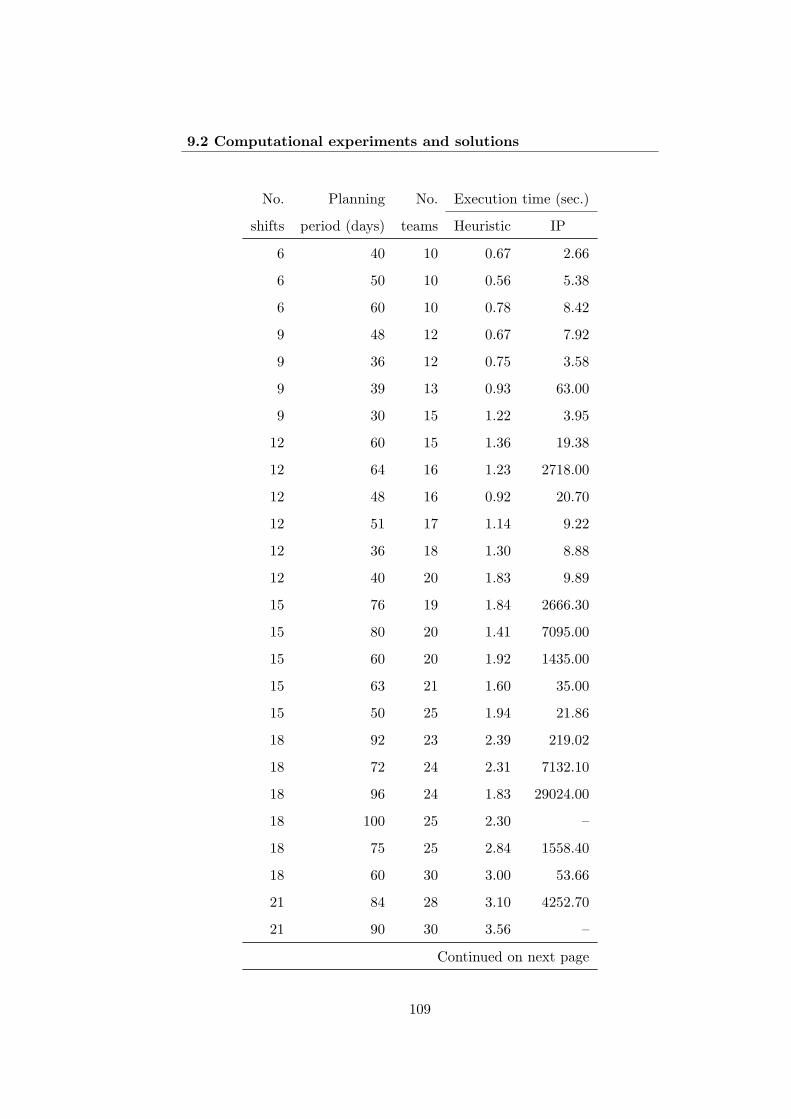
9.2 Computational experiments and solutions
No. Planning No. Execution time (sec.)
shifts period (days) teams Heuristic IP
6 40 10 0.67 2.66
6 50 10 0.56 5.38
6 60 10 0.78 8.42
9 48 12 0.67 7.92
9 36 12 0.75 3.58
9 39 13 0.93 63.00
9 30 15 1.22 3.95
12 60 15 1.36 19.38
12 64 16 1.23 2718.00
12 48 16 0.92 20.70
12 51 17 1.14 9.22
12 36 18 1.30 8.88
12 40 20 1.83 9.89
15 76 19 1.84 2666.30
15 80 20 1.41 7095.00
15 60 20 1.92 1435.00
15 63 21 1.60 35.00
15 50 25 1.94 21.86
18 92 23 2.39 219.02
18 72 24 2.31 7132.10
18 96 24 1.83 29024.00
18 100 25 2.30 –
18 75 25 2.84 1558.40
18 60 30 3.00 53.66
21 84 28 3.10 4252.70
21 90 30 3.56 –
Continued on next page
109
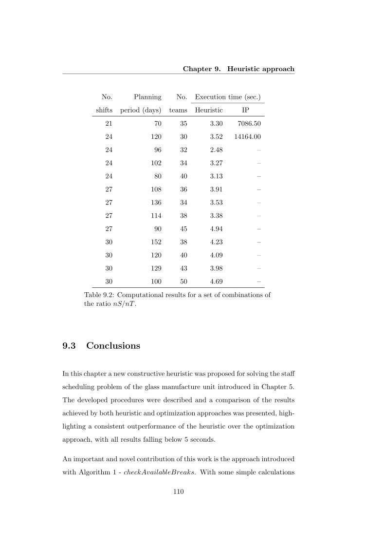
Chapter 9. Heuristic approach
No. Planning No. Execution time (sec.)
shifts period (days) teams Heuristic IP
21 70 35 3.30 7086.50
24 120 30 3.52 14164.00
24 96 32 2.48 –
24 102 34 3.27 –
24 80 40 3.13 –
27 108 36 3.91 –
27 136 34 3.53 –
27 114 38 3.38 –
27 90 45 4.94 –
30 152 38 4.23 –
30 120 40 4.09 –
30 129 43 3.98 –
30 100 50 4.69 –
Table 9.2: Computational results for a set of combinations ofthe ratio nS/nT .
9.3 Conclusions
In this chapter a new constructive heuristic was proposed for solving the staff
scheduling problem of the glass manufacture unit introduced in Chapter 5.
The developed procedures were described and a comparison of the results
achieved by both heuristic and optimization approaches was presented, high-
lighting a consistent outperformance of the heuristic over the optimization
approach, with all results falling below 5 seconds.
An important and novel contribution of this work is the approach introduced
with Algorithm 1 - checkAvailableBreaks. With some simple calculations
110

9.3 Conclusions
over the problem’s input data, it is possible to foresee the existence of a
feasible solution. Although the proposed heuristic was developed for this
specific instance, it is flexible enough to account for variations in some of
the problem’s parameters and constraints. That is the case of the sequence
of working shifts, which can be any that the user defines, as well as the
minimum and maximum number of consecutive working days. With slight
adjustments, the number of breaks to interpose between working blocks
can also be redefined. Nevertheless, the proposed procedure has limitations
when considering its direct applicability to other instances. It imposes the
existence of at least one break day between each change of working shifts, so
it does not allow for the possibility of having different shifts on consecutive
days. The shift daily demand, for example, is a very strong constraint of this
particular problem since it is on the basis of the calculation of the number
of available breaks, as it was previously explained, which is a conditioning
factor for the existence of a feasible solution. In problems with more than
one team working simultaneously on the same shift, or with different daily
requirements for each shift, this constraint would have to be reformulated
and would imply deeper adjustments in the procedures proposed, but the
base reasoning would be the same. As stated before, the “working-shifts
sequence” approach is a strength of this work, for problems where a unique
predefined sequence must be followed. But it can also be a limitation be-
cause, in problems where a set of sequences should be avoided, the heuristic
may not respond accordingly, unless a preferred sequence can be chosen.
As a conclusion, we believe that the achieved results are promising and
encouraging of further extensions of the heuristic in order to consider, for
example, different shift daily demands or forbidden sequences of shifts.
111

Chapter 9. Heuristic approach
112

Chapter 10
Conclusions
10.1 Contributions of this work
In this thesis, we proposed an optimization method for simultaneously as-
signing work shifts and days-off to each employee. A general IP model was
developed and applied, with slight adjustments, to three real-world prob-
lems: a glass production unit, a continuous care unit and a hospital. A set
of benchmark instances was also used in order to evaluate the model’s per-
formance when solving larger problems and to compare results with other
methods. Two main goals of the model were to ensure a balanced and eq-
uitable schedule between all employees, in terms of workload, and also to
respect a predefined sequence of work shifts and days-off, either following
work rules or employees’ preferences. The first goal was achieved, initially,
through the levelling of the number of days that each team works in each
shift, as imposed by the objective function defined for the general model and
in a next phase, through the imposition of equal schedules to all employ-
ees, with a time lag, of a predefined number of days, between them. This
feature gives a cyclic dimension to the schedule. The second condition was
achieved through the formulation of an array of indices that, together with
the definition of a maximum and a minimum number of consecutive days,
113

Chapter 10. Conclusions
enable the imposition of any desired pattern of work shifts and days-off.
This pattern can be the same for all employees or can be defined according
to contract types, skills, employees preferences, etc. This original formu-
lation also makes it possible to control the periodicity of days-off, as well
as the length of the tour or sub-period of the planning horizon. The defi-
nition of the planning period is not a very explored issue in the literature,
since it is closely related to demand forecast periods and it is often an input
parameter. But the initially set planning period may not be the one that
better fits the problem’s features and so it is pertinent to study which is the
“ideal” planning period for a specific instance. This experiment was carried
out. Even though constraints on the periodicity of long-weekends and on
planned absences were not an initial issue, the model was able to handle
them as well, as shown in two of the case-studies.
The model developed in this work demonstrated to be general and flexible,
with several degrees of freedom and with the capacity of being easily applied
to different real-life staff scheduling problems, but at the same time with a
cyclic feature that ensures the equitableness and predictability of the sched-
ule. The cyclic approach, often considered to be inflexible and not easily
adjustable, proved to be flexible enough to successfully solve problems that
are typically addressed with acyclic scheduling, namely with heterogeneous
staff and fluctuating demand levels. This is a new insight and represents a
novel contribution to the academic literature.
From a company’s point of view, the use of the automatic scheduling model
proposed in this research work can represent a powerful tool for increasing
both the efficiency and the effectivity of the staff scheduling process, leading
to higher profitability and productivity. However, the implementation of
such a solution into practice is not always easy, it deeply depends on the
involvement of the company in the whole development process.
114

10.2 Future research directions
The developed heuristic approach represents an alternative method for solv-
ing one of the real-world problems studied in this thesis, allowing also for a
comparative evaluation of the optimization model’s performance. An origi-
nal contribution of the heuristic is that with some simple calculations over
the problem’s input data, it is possible to foresee the existence of a feasible
solution. This reduces the solution search space.
Additionally, the comprehensive study on the staff scheduling problem and
the insight into hospitality management operations constitute two assets for
researchers looking for background on these topics.
As a conclusion, we proposed a generic, novel and valuable approach to
staff scheduling. We developed generic methodologies, showed their flexibil-
ity and solved a set of different problems. We challenged the potential of
cyclic scheduling and proved it can be flexible. We developed an innovative
formulation of sequence and consecutiveness of shifts. And we believe this
research work can add value to a company by leading to cost reduction and
an increase in the productivity.
10.2 Future research directions
In order to consolidate our findings, future research could address the appli-
cation of the proposed IP model to more real-world problems, from different
activity sectors. Hospitality management is a promising area that should be
more explored, namely hotels (housekeeping staff) and restaurants.
Concerning the problems’ features, all the problems studied in this work
had fixed shifts. It would be interesting to extend the IP model to consider
the case of variable shifts, in terms of starting-times, length or even the
placement of breaks.
One of the drawbacks that are usually pointed out in the literature to cyclic
115

Chapter 10. Conclusions
scheduling approaches is their difficulty in handling non predicted absences.
In Chapter 5 absentees were replaced within their team. We have also shown
how the IP model can ocasionally accommodate planned absences (Chapter
7). A systematic way of addressing this constraint could be worthy of further
research.
Although the proposed heuristic was developed for a specific problem, it
proved to be flexible enough to account for variations in some of the prob-
lem’s parameters and constraints. The achieved results encourage further
extensions of the procedure in order to consider, for example, different shift
daily demands or forbidden sequences of shifts.
116

References
Abdennadher, S. and Schlenker, H. (1999). Nurse scheduling using con-
straint logic programming. In Proceedings of the 11th Conference on In-
novative Applications of Artificial Intelligence, pages 838–843.
Addou, I. and Soumis, F. (2007). Bechtold-Jacobs generalized model for shift
scheduling with extraordinary overlap. Annals of Operations Research,
155:177–205.
Aickelin, U. and White, P. (2004). Building Better Nurse Scheduling Algo-
rithms. Annals of Operations Research, 128(1-4):159–177.
Alfares, H. (2004). Survey, categorization, and comparison of recent tour
scheduling literature. Annals of Operations Research, 127(1):145–175.
Alfares, H. K. (1998). An efficient two-phase algorithm for cyclic days-off
scheduling. Computers & Operations Research, 25(11):913 – 923.
Antunes, A. F. and Moz, M. (2011). Optimizacao do escalonamento de en-
fermeiros numa unidade hospitalar. In INESC-COIMBRA, editor, Livro
de Actas do 15 Congresso da Associacao Portuguesa de Investigacao Op-
eracional (IO2011), pages 25–36.
Arabeyre, J., Fearnley, J., Steiger, F., and Teather, W. (1969). The airline
crew scheduling problem: A survey. Transportation Science, 3(2):140–163.
Aykin, T. (2000). A comparative evaluation of modeling approaches to the
117

REFERENCES
labor shift scheduling problem. European Journal of Operational Research,
125(2):381–397.
Azaiez, M. (2005). A 0-1 goal programming model for nurse scheduling.
Computers & Operations Research, 32(3):491–507.
Baker, K. R. (1976). Workforce Allocation in Cyclical Scheduling Problems:
A Survey. Operational Research Quarterly (1970-1977), 27(1):155.
Balakrishnan, N. and Wong, R. T. (1990). A network model for the rotating
workforce scheduling problem. Networks, 20:25–42.
Bard, J. F., Binici, C., and DeSilva, A. H. (2003). Staff scheduling at
the United States Postal Service. Computers & Operations Research,
30(5):745–771.
Barros, C. P. and Mascarenhas, M. J. (2005). Technical and allocative
efficiency in a chain of small hotels. International Journal of Hospitality
Management, 24(3):415 – 436.
Barros, C. P., Peypoch, N., and Solonandrasana, B. (2008). Efficiency and
productivity growth in hotel industry. International Journal of Tourism
Research.
Beaulieu, H., Ferland, J. A., Gendron, B., and Michelon, P. (2000). A mathe-
matical programming approach for scheduling physicians in the emergency
room. Health care management science, 3(3):193–200.
Beaumont, N. (1997). Using mixed integer programming to design employee
rosters. Journal of the Operational Research Society, 48(6):585–590.
Bechtold, S. and Jacobs, L. (1990). Implicit modeling of flexible break as-
signments in optimal shift scheduling. Management Science, 36(11):1339–
1351.
118
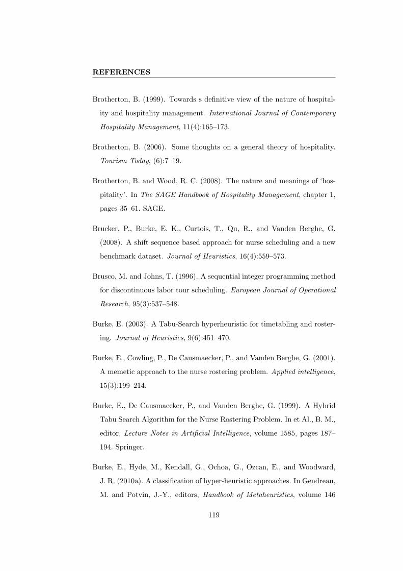
REFERENCES
Brotherton, B. (1999). Towards s definitive view of the nature of hospital-
ity and hospitality management. International Journal of Contemporary
Hospitality Management, 11(4):165–173.
Brotherton, B. (2006). Some thoughts on a general theory of hospitality.
Tourism Today, (6):7–19.
Brotherton, B. and Wood, R. C. (2008). The nature and meanings of ‘hos-
pitality’. In The SAGE Handbook of Hospitality Management, chapter 1,
pages 35–61. SAGE.
Brucker, P., Burke, E. K., Curtois, T., Qu, R., and Vanden Berghe, G.
(2008). A shift sequence based approach for nurse scheduling and a new
benchmark dataset. Journal of Heuristics, 16(4):559–573.
Brusco, M. and Johns, T. (1996). A sequential integer programming method
for discontinuous labor tour scheduling. European Journal of Operational
Research, 95(3):537–548.
Burke, E. (2003). A Tabu-Search hyperheuristic for timetabling and roster-
ing. Journal of Heuristics, 9(6):451–470.
Burke, E., Cowling, P., De Causmaecker, P., and Vanden Berghe, G. (2001).
A memetic approach to the nurse rostering problem. Applied intelligence,
15(3):199–214.
Burke, E., De Causmaecker, P., and Vanden Berghe, G. (1999). A Hybrid
Tabu Search Algorithm for the Nurse Rostering Problem. In et Al., B. M.,
editor, Lecture Notes in Artificial Intelligence, volume 1585, pages 187–
194. Springer.
Burke, E., Hyde, M., Kendall, G., Ochoa, G., Ozcan, E., and Woodward,
J. R. (2010a). A classification of hyper-heuristic approaches. In Gendreau,
M. and Potvin, J.-Y., editors, Handbook of Metaheuristics, volume 146
119

REFERENCES
of International Series in Operations Research & Management Science,
pages 449–468. Springer US.
Burke, E. K., De Causmaecker, P., Vanden Berghe, G., and Van Landeghem,
H. (2004). The State of the Art of Nurse Rostering. Journal of Scheduling,
7(6):441–499.
Burke, E. K., Li, J., and Qu, R. (2010b). A hybrid model of integer program-
ming and variable neighbourhood search for highly-constrained nurse ros-
tering problems. European Journal of Operational Research, 203(2):484–
493.
Carrasco, R. C. (2010). Long-term staff scheduling with regular temporal
distribution. Computer methods and programs in biomedicine, 100(2):191–
9.
Castillo, I., Joro, T., and Li, Y. (2009). Workforce scheduling with multiple
objectives. European Journal of Operational Research, 196(1):162–170.
Cezik, T., Gunluk, O., and Luss, H. (2001). An integer programming
model for the weekly tour scheduling problem. Naval Research Logistics,
48(7):607–624.
Chan, P., Weil, G., Cosytec, S. A., Rostand, R. J., and Orsay-universite,
P. C. (2001). Cyclical Staff Scheduling Using Constraint Logic Program-
ming. Practice and Theory of Automated Timetabling III - 3rd Interna-
tional Conference, PATAT 2000, Konstanz, Germany, pages 159–175.
Choi, K., Hwang, J., and Park, M. (2009). Scheduling Restaurant Workers
to Minimize Labor Cost and Meet Service Standards. Cornell Hotel and
Restaurant Administration Quarterly, 50(2):155.
Constantino, A. A., de Melo, E. L., Landa-Silva, D., and Romao, W. (2011).
A heuristic algorithm for nurse scheduling with balanced preference sat-
120
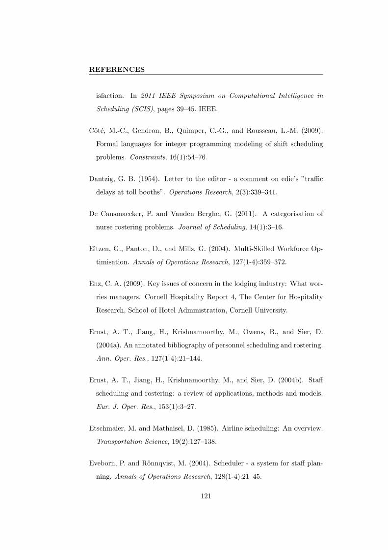
REFERENCES
isfaction. In 2011 IEEE Symposium on Computational Intelligence in
Scheduling (SCIS), pages 39–45. IEEE.
Cote, M.-C., Gendron, B., Quimper, C.-G., and Rousseau, L.-M. (2009).
Formal languages for integer programming modeling of shift scheduling
problems. Constraints, 16(1):54–76.
Dantzig, G. B. (1954). Letter to the editor - a comment on edie’s ”traffic
delays at toll booths”. Operations Research, 2(3):339–341.
De Causmaecker, P. and Vanden Berghe, G. (2011). A categorisation of
nurse rostering problems. Journal of Scheduling, 14(1):3–16.
Eitzen, G., Panton, D., and Mills, G. (2004). Multi-Skilled Workforce Op-
timisation. Annals of Operations Research, 127(1-4):359–372.
Enz, C. A. (2009). Key issues of concern in the lodging industry: What wor-
ries managers. Cornell Hospitality Report 4, The Center for Hospitality
Research, School of Hotel Administration, Cornell University.
Ernst, A. T., Jiang, H., Krishnamoorthy, M., Owens, B., and Sier, D.
(2004a). An annotated bibliography of personnel scheduling and rostering.
Ann. Oper. Res., 127(1-4):21–144.
Ernst, A. T., Jiang, H., Krishnamoorthy, M., and Sier, D. (2004b). Staff
scheduling and rostering: a review of applications, methods and models.
Eur. J. Oper. Res., 153(1):3–27.
Etschmaier, M. and Mathaisel, D. (1985). Airline scheduling: An overview.
Transportation Science, 19(2):127–138.
Eveborn, P. and Ronnqvist, M. (2004). Scheduler - a system for staff plan-
ning. Annals of Operations Research, 128(1-4):21–45.
121
REFERENCES
Gans, N., Koole, G., and Mandelbaum, A. (2003). Telephone call centers:
Tutorial, review, and research prospects. Manufacturing and service op-
erations management, 5(2):79–141.
Glass, C. A. and Knight, R. A. (2010). The nurse rostering problem: A crit-
ical appraisal of the problem structure. European Journal of Operational
Research, 202(2):379–389.
Glover, F. (1986). The general employee scheduling problem. An integration
of MS and AI. Computers & Operations Research, 13(5):563–573.
Gopalakrishnan, B. and Johnson, E. L. (2005). Airline Crew Scheduling:
State-of-the-Art. Annals of Operations Research, 140(1):305–337.
Hao, G. and Lai, K. (2004). A neural network application in personnel
scheduling. Annals of Operations Research, pages 65–90.
Hemmington, N. (2007). From service to experience: Understanding and
defining the hospitality business. Serv. Ind. J., 27(6):747–755.
HMI (2008). Hospitality management institute.
http://www.hmiportugal.com/.
“hospitality” (2011a). The American Heritage R© Dictionary of the
English Language, Fourth Edition, Retrieved May 19 2011 from
http://www.thefreedictionary.com/hospitality.
“hospitality” (2011b). Collins Essential English Dic-
tionary, 2nd Edition, Retrieved May 19 2011 from
http://www.thefreedictionary.com/hospitality.
Isken, M. W. (2004). An Implicit Tour Scheduling Model with Applications
in Healthcare. Annals of Operations Research, 128(1-4):91–109.
Jones, P. (1996). Hospitality research - where have we got to? International
Journal of Hospitality Management, 15(1):5–10.
122

REFERENCES
Jones, P. (2004). Finding the hospitality industry? or finding hospitality
schools of thought? Journal of Hospitality, Leisure, Sport and Tourism
Education, 3(1):33–45.
Keith, E. (1979). Operator scheduling. IIE Transactions, 11(1):37–41.
King, C. A. (1995). What is hospitality? International Journal of Hospitality
Management, 14(3-4):219 – 234.
Kohl, N. and Karisch, S. E. (2004). Airline Crew Rostering: Problem
Types, Modeling, and Optimization. Annals of Operations Research,
127(1-4):223–257.
Laporte, G. (1999). The art and science of designing rotating schedules. The
Journal of the Operational Research Society, 50(10):1011–1017.
Laporte, G. and Pesant, G. (2004). A general multi-shift scheduling system.
Journal of the Operational Research Society, 55(11):1208–1217.
Lashley, C. (2008). Studying hospitality: Insights from social sciences. Scan-
dinavian Journal of Hospitality and Tourism, 8(1):69–84.
Lashley, C. and Morrison, A. J. (2000). In Search of Hospitality: Theoretical
Perspectives and Debates. Oxford: Butterworth-Heinemann.
Loucks, J. and Jacobs, F. (1991). Tour scheduling and task assignment
of a heterogeneous work force: A heuristic approach. Decision Sciences,
22(4):719–738.
Love, R. L. and Hoey, J. (1990). Management science improves fast-food
operations. Interfaces, 20(2):21–29.
Ministry for Economy and Innovation (2011). National Strategic Plan for
Tourism - Revision Proposal for 2015 (v2.0). Retrieved June 20 2012 from
http://www.turismodeportugal.pt.
123

REFERENCES
Misir, M., Verbeeck, K., De Causmaecker, P., and Vanden Berghe, G. (2010).
Hyper-heuristics with a dynamic heuristic set for the home care scheduling
problem. In Evolutionary Computation (CEC), 2010 IEEE Congress on,
pages 1–8. IEEE.
Mora, M. and Musliu, N. (2004). Genetic algorithm for rotating workforce
scheduling problem. In Computational Cybernetics, 2004. ICCC 2004.
Second IEEE International Conference on, pages 121–126. IEEE.
Moz, M. and Pato, M. V. (2004). Solving the problem of rerostering nurse
schedules with hard constraints: new multicommodity flow models. An-
nals of Operations Research, (1976):179–197.
Musliu, N. (2006). Heuristic Methods for Automatic Rotating Workforce
Scheduling. International Journal of Computational Intelligence Research,
2(4):309–326.
Ottenbacher, M., Harrington, R., and Parsa, H. (2009). Defining the Hospi-
tality Discipline: a Discussion of Pedagogical and Research Implications.
Journal of Hospitality & Tourism Research, 33(3):263.
Qu, R. and He, F. (2009). A Hybrid Constraint Programming Approach
for Nurse Rostering Problems. In Allen, T and Ellis, R and Petridis, M,
editor, Applications and Innovations in Intelligent Systems XVI, pages
211–224. Springer-Verlag London Ltd. 28th SGAI International Confer-
ence on Innovative Techniques and Applications of Artificial Intelligence,
Cambridge, England.
Rekik, M., Cordeau, J.-F., and Soumis, F. (2010). Implicit shift scheduling
with multiple breaks and work stretch duration restrictions. Journal of
Scheduling, 13(1):49–75.
Rong, A. (2010). Monthly tour scheduling models with mixed skills con-
124

REFERENCES
sidering weekend off requirements. Computers & Industrial Engineering,
59(2):334–343.
Sellmann, M., Zervoudakis, K., Stamatopoulos, P., and Fahle, T. (2000).
Integrating Direct CP Search and CP-based Column Generation for the
Airline Crew Assignment Problem. In Transportation Science, number 24,
pages 163–170.
Silvestro, R. and Silvestro, C. (2001). An evaluation of nurse rostering
practices in the National Health Service. Journal of Advanced Nursing,
32(3):525–535.
Slattery, P. (2002). Finding the hospitality industry. Journal of Hospitality,
Leisure, Sport and Tourism Education, 1(1):19–28.
Taylor, S. and Edgar, D. (1996). Hospitality research: the emperor’s new
clothes? International Journal of Hospitality Management, 15(3):211–
227.
Thompson, G. (1996). Controlling Action Timnes in Daily Workforce Sched-
ules. Cornell Hotel and Restaurant Administration Quarterly, 37(2):82.
Thompson, G. (1998a). Labor scheduling, part 1: Forecasting demand.
Cornell Hotel and Restaurant Administration Quarterly, 39(5):22.
Thompson, G. (1998b). Labor scheduling, part 2: Knowing how many on-
duty employees to schedule. Cornell Hotel and Restaurant Administration
Quarterly, 39(6):26–37.
Thompson, G. (1999a). Labor scheduling, part 3: Developing a work-
force schedule. Cornell Hotel and Restaurant Administration Quarterly,
40(1):86.
Thompson, G. (1999b). Labor Scheduling, Part 4: Controlling Workforce
125

REFERENCES
Schedules in Real Time. Cornell Hotel and Restaurant Administration
Quarterly, 40(3):85.
Thompson, G. M. (2003). Labor Scheduling: A Commentary. Cornell
Hospitality Quarterly, 44(5-6):149–155.
Thompson, G. M. and Goodale, J. C. (2006). Variable employee productiv-
ity in workforce scheduling. European Journal of Operational Research,
170(2):376 – 390.
Topaloglu, S. and Ozkarahan, I. (2004). An Implicit Goal Programming
Model for the Tour Scheduling Problem Considering the Employee Work
Preferences. Annals of Operations Research, 128(1-4):135–158.
Totterdell, P. (2005). Work schedules. Handbook of work stress, page 53.
Ulusam Seckiner, S., Gokcen, H., and Kurt, M. (2007). An integer pro-
gramming model for hierarchical workforce scheduling problem. European
Journal of Operational Research, 183(2):694–699.
Valouxis, C. and Housos, E. (2000). Hybrid optimization techniques for the
workshift and rest assignment of nursing personnel. Artificial intelligence
in medicine, 20(2):155–75.
Van den Bergh, J., Belien, J., De Bruecker, P., Demeulemeester,
E., and De Boeck, L. (2012). Personnel scheduling: A
literature review. European Journal of Operational Research,
http://dx.doi.org/10.1016/j.ejor.2012.11.029.
Warner, D. M. (1976). Scheduling nursing personnel according to nursing
preference: a mathematical programming approach. Operations Research,
24(5).
Wren, A. (1996). Scheduling, timetabling and rostering - a special rela-
tionship? In Selected papers from the First International Conference on
126
REFERENCES
Practice and Theory of Automated Timetabling, pages 46–75, London,
UK. Springer-Verlag.
Wren, A. (1998). Heuristics ancient and modern: Transport scheduling
through the ages. Journal of Heuristics, 4:87–100.
Wren, A. and Rousseau, J. (1995). Bus driver scheduling - an overview.
Technical Report July, University of Leeds, School of Computer Studies.
127