1

VIBRATION OF CONTINUOUS SYSTEMS

Dr S. Talukdar

Professor

Department of Civil Engineering

Indian Institute of Technology Guwahati-781039

INTRODUCTION

Modeling the structures with discrete coordinates provides a practical approach for the

analysis of structures subjected to dynamic loads. However, the results obtained from

these discrete models can only give approximate solutions to the actual behaviour. The

present lectures consider the dynamic theory of beams and rods having distributed mass

and elasticity for which governing equations of motion are partial differential equations.

The integration of these equations is in general more complicated than the solution of

ordinary differential equations governing discrete dynamic systems. Due to this

mathematical complexity, the dynamic analysis of structures as continuous systems has

limited use in practice. Nevertheless, the analysis as continuous systems of some generic

models of structures provides very useful information of the overall dynamic behaviour

of structures. The method of analysis of continuous system is illustrated with examples of

torsional, axial and bending vibration of beams. For, beams with non uniform geometry,

closed form solution is very much involved. In such case, approximate methods (such as

Rayleigh Ritz method or Gallerkin Method) can be used.

EQUATION OF MOTIONS

The of equations of motion can be derived by (i) force balance of a differential element

(ii) Hamilton’s principle (iii) Lagranges method. While the force balance is a convenient

approach for most of the problems, Hamiltons principle and Lagranges method are

applied for a complex system. These two approaches need the consideration of the energy

of the system.

Hamilton’s Principle

Hamilton’s principle is stated as an integral equation in which the energy is integrated

over an interval of time. Mathematically, the principle can be stated as

∫ ∫ ==−2

1

2

1

0)(

t

t

t

t

LdtdtVT δδ (1)

where L is the Lagrangian, T and V are kinetic and potential energy of the system. The

physical interpretation of the eq.(1) is that out of all possible paths of motion of a system

during an interval of time from t1 to t2 , the actual path will be that for which the integral

∫t

Ldt has a stationary value. It can be shown that in fact stationary value will, in fact, the

minimum value of the integral.

2

The Hamilton’s principle can yield the governing differential equations as well as

boundary conditions.

Lagrange’s Equation

Hamilton’s principle is stated as an integral equation where total energy is integrated over

an time interval. On the other hand, Lagrange’s equation is differential equations, in

which one considers the energies of the system instantaneously in time. Hamilton’s

principle can be used to derive the Lagrange’s equation in a set of generalized

coordinates. Lagrange’s equation may be written as

0=∂∂

−

∂∂

ii q

L

q

L

dt

d (2)

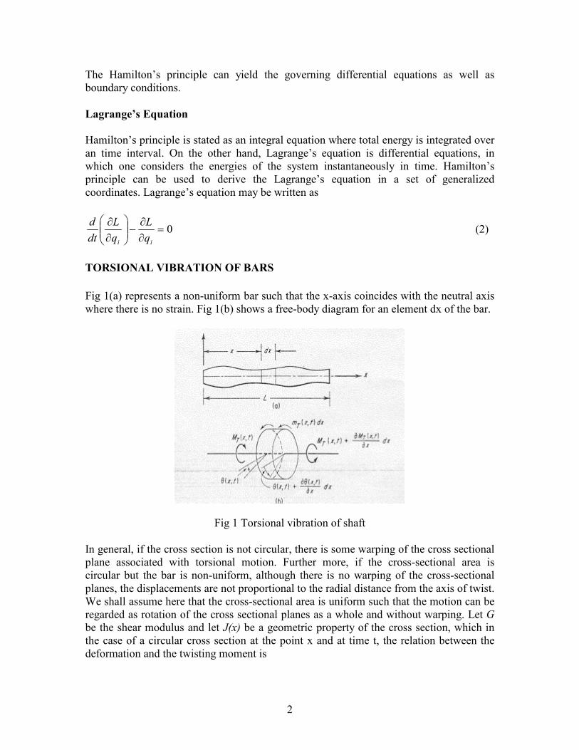
TORSIONAL VIBRATION OF BARS

Fig 1(a) represents a non-uniform bar such that the x-axis coincides with the neutral axis

where there is no strain. Fig 1(b) shows a free-body diagram for an element dx of the bar.

Fig 1 Torsional vibration of shaft

In general, if the cross section is not circular, there is some warping of the cross sectional

plane associated with torsional motion. Further more, if the cross-sectional area is

circular but the bar is non-uniform, although there is no warping of the cross-sectional

planes, the displacements are not proportional to the radial distance from the axis of twist.

We shall assume here that the cross-sectional area is uniform such that the motion can be

regarded as rotation of the cross sectional planes as a whole and without warping. Let G

be the shear modulus and let J(x) be a geometric property of the cross section, which in

the case of a circular cross section at the point x and at time t, the relation between the

deformation and the twisting moment is

3

( ) ( ) ( )x

txxGJtxM T ∂∂

=,

,θ

(3)

Where the product GJ (x) is called torsional stiffness.

Let I (x) be the moss polar moment of inertia per unit length of bar mT (x,t) be the

external twisting moment per unit length of bar.

The rotational motion of the bar element in the form

( )2

2 ),()(),(),(

),(,

t

txdxxItxMdxtxmdx

x

txMtxM TT

TT ∂

∂=−+

∂

∂+

θ (4)

which reduces to

2

2 ),()(),(

),(

t

txdxxItxm

x

txMT

T

∂

∂=+

∂

∂ θ (5)

In view of equation (3), we can write equation (5) as

x∂∂

2

2 ),()(),(

),()(

t

txdxxItxm

x

txxGJ T ∂

∂=+

∂

∂ θθ (6)

which is equation of motion in torsion.

In the case in which mT (x,t) = 0, (6) reduces to the equation for the free torsional

vibration of a bar,

x∂∂

2

2 ),()(

),()(

t

txdxxI

x

txxGJ

∂

∂=

∂

∂ θθ (7)

For a clamped end at x = 0, we obtain the boundary condition

θ(0,t)= 0, (8)

and for a free end at x = L the boundary condition is

Lxx

txxGJ

=∂∂ ),()(

θ=0, (9)

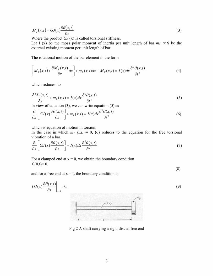
Fig 2 A shaft carrying a rigid disc at free end

4

Example: Calculation of Natural Frequency of Torsional vibration

Consider a circular bar with a rigid disk attached at one end. The torsional rigidity of the

bar is GJ(x), its mass polar moment of inertia per unit length is I(x), and the mass polar

moment of the disk is ID (Fig 2).

Boundary conditions, x = 0 we have

0),( =txθ at x=0

Lxx

txxGJ

=∂∂ ),()(

θ= −

Lx

Dt

txI

=∂

∂2

2 ),(θ (10)

Let )()(),( tfxtx φθ = (11)

Recalling that f(t) is harmonic, the igenvalue problem reduces to the differential equation

)()()(

)( 2 xxIdx

xdxGJ

dx

dφω

φ=

− (12)

to be satisfied throughout the domain 0< x <L, and the boundary conditions

φ(0) = 0, (13)

)(),(

)( 2 xIx

txxGJ D

Lx

φωφ

=∂

∂

=

(14)

at the ends.

For uniform shaft, we have

22

βω

=GJ

I (15)

So that the equation (12) reduces to

,0)()( 2

2

2

=+ xdx

xdφβ

φ (16)

which has the solution

xCxCx ββφ sincos)( 21 += (17)

From boundary condition eq.(13), it follows that C2 = 0. Boundary condition (14) gives

Thus, the frequency equation is obtained as

LCILGJC D βωββ sincos 1

2

1 =

LI

ILL

D ββ

1tan = (18)

5

This is a transcendental equation in βL. It has infinite number of solutions βL which must be obtained numerically and are related to the natural frequencies ωt by

,2IL

GJLrr βω = r = 1,2… (19)

Note that ,2IL

GJLrr βω = the natural frequencies ωr are no longer integral multiples of

the fundamental frequency ω1

Natural modes are given by

,sin)( xAx rrr βφ = r,s = 1,2,……..; r≠s (20)

They are orthogonal functions. The orthognality condition follows

,0)()()()(0

=+∫ LLIdxxxI srDsr

L

φφφφ r = 1,2,……. (21)

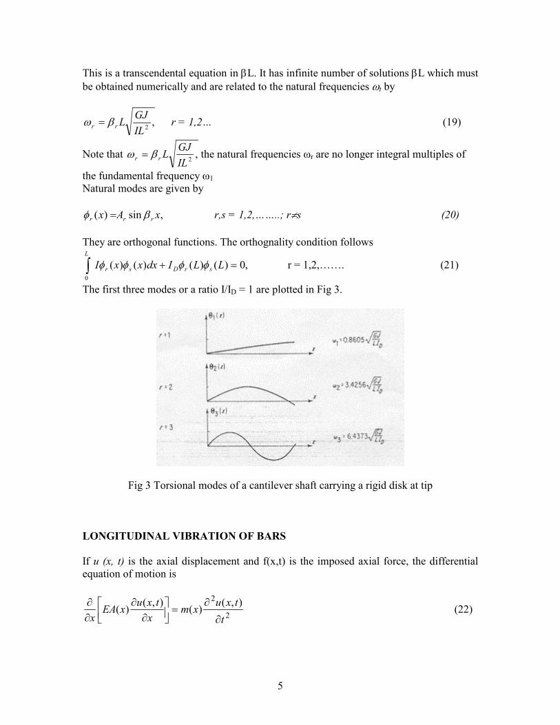
The first three modes or a ratio I/ID = 1 are plotted in Fig 3.

Fig 3 Torsional modes of a cantilever shaft carrying a rigid disk at tip

LONGITUDINAL VIBRATION OF BARS

If u (x, t) is the axial displacement and f(x,t) is the imposed axial force, the differential

equation of motion is

2

2 ),()(

),()(

t

txuxm

x

txuxEA

x ∂

∂=

∂

∂∂∂

(22)

6

The equation must be satisfied over the domain 0 < x < L. In addition, u must be such

that at the end points we have

00=∂

∂∂ l

ux

uEA (23)

If the bar is clamped at the end x=0, the boundary condition is

( ) ,0,0 =tu (24)

and if the end x = l is free, we have

.0),(

)( =∂

∂

=lxx

txuxEA (25)

The nature of the differential equation of motion is similar to that of torsional vibration of

circular shaft ignoring warping.

Example: Calculation of Natural Frequencies of Axial Vibration

Let us consider a clamped-free rod, for which the eigen-value problem reduces to the

solution of the differential equation

Let )()(),( tfxUtxu = where U(x) is the mode shape and f(t) is a harmonic function.

),()()(

)( 2 xUxmdx

xdUxEA

dx

dϖ=

− (26)

This must be satisfied throughout the domain, and the homogeneous boundary conditions

,0)0( =U (27)

,0)(

)( ==Lxdx

xdUxEA (28)

to be satisfied at the end point.

For a uniform rod the eigenvalue problem reduces to the solution of the differential

equation

,0)()( 2

2

2

=+ xUdx

xUdβ ,22

EA

mωβ = (29)

which is subject to boundary conditions (27) and (28). The solution of (29) is

.cossin)( 21 xCxCxU ββ += (30)

7

Boundary conditions (27) yields C2 = 0, and from boundary conditions (28) we obtain the

frequency equation

0cos =Lβ , (31)

Which yields the eigenvalues

,2)12(L

rr

πβ −= r = 1,2,.., (32)

so that the natural frequencies ϖr are

,2)12(

2mL

EAr

m

EA

rr

πβϖ −== r = 1,2,.., (33)

The corresponding eigen functions have the form

,2)12sin()(

L

xrAxU rr

π−= r = 1,2,.., (34)

and they are orthogonal. Let us normalize them and adjust the coefficients Ar such that

,1)()(0

=∫ dxxUxmU sL

r for r=s and 0 for r≠s (35)

From which we obtain the orthonormal set

,2)12sin(

2)(

L

xr

mLxU r

π−= r = 1,2,.., (36)

The first three modes are shown in Figure 4

Fig 4 Mode shapes in Axial vibration of Clamped-Free bar

8

Let us consider a case in which both ends are free. The formulations follows the same

pattern and once again we find that homogeneous equation must be satisfied through-out

the domain 0 < x < L, but in contrast to the previous case the boundary conditions in this

case are

0)(

)(0

==xdx

xdUxEA (37)

0)(

)( ==Lxdx

xdUxEA

This problem is self-adjoint and semi definite. Letting the rod be uniform, yield C1 = 0,

whereas boundary conditions in (37) gives the frequency equation

,0sin =Lβ (38)

Which leads to the eigen values

,l

rr

πβ = r = 0,1,2,…, (39)

Here βo = 0 is also an eigenvalue, incorporating an earlier statement made in connection with semi definite systems. Corresponding to the eigenvalues other than βo we have the eigenfunctions

,cos)(L

xrAxU rr π= r = 1,2,…. (40)

For β = βo = 0, the equation becomes

,0)(

2

2

=dx

xUd (41)

which has the solution

.)( ' xAAxU ooo += (42)

Upon consideration of the boundary conditions, it reduces to

oo AxU =)( (43)

Hence to the eigen values β = βo = 0 there corresponds a mode that is interpreted as the displacement of the rod as a whole. This is known as a rigid-body mode and is typical of

under restrained systems (semi definite systems) for which there are no forces or moment

exerted by the supports. In this particular case we are concerned with forces in the

longitudinal direction only and not with moments. Denoting the resultant force in the

longitudinal direction F (t) we have

∫ ∫ ==∂

∂=

L

o

L

dxxUxmtfdxt

txUxmtF

0

2

2

0)()()(),(

)()( �� (44)

Because there is no external force present. The above leads to the equations

9

0)()(0

=∫ dxxUxm

L

r r = 1,2,… (45)

Which can be merely interpreted as the statement of the fact that the rigid body mode is

orthogonal to the elastic modes .The orthogonality relation and the normalization

statement may be combined in to

rss

L

r dxxUxUxm δ=∫ )()()(0

r, s = 0,1,2… (46)

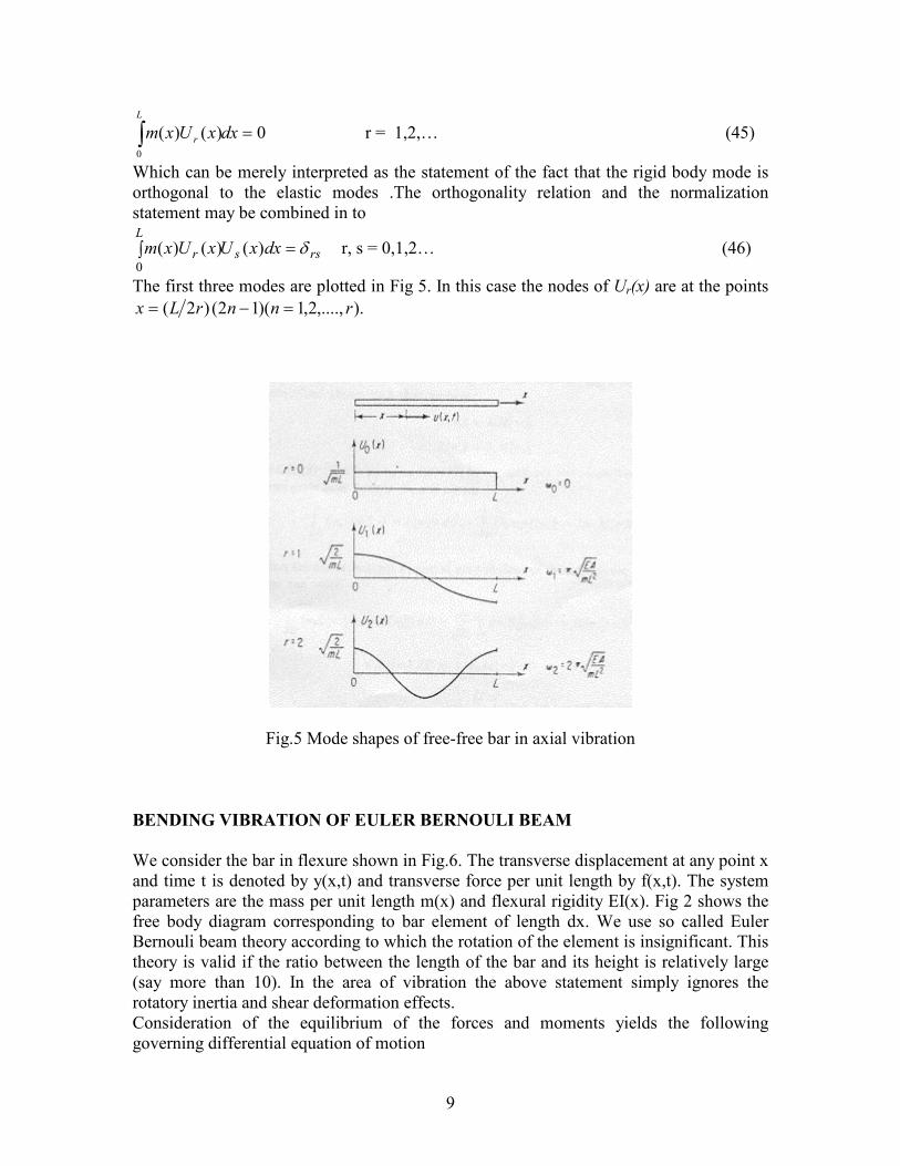
The first three modes are plotted in Fig 5. In this case the nodes of Ur(x) are at the points

).,....,2,1)(12()2( rnnrLx =−=

Fig.5 Mode shapes of free-free bar in axial vibration

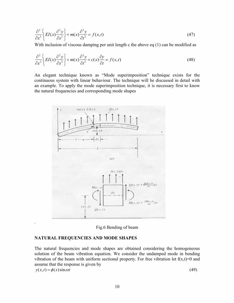
BENDING VIBRATION OF EULER BERNOULI BEAM

We consider the bar in flexure shown in Fig.6. The transverse displacement at any point x

and time t is denoted by y(x,t) and transverse force per unit length by f(x,t). The system

parameters are the mass per unit length m(x) and flexural rigidity EI(x). Fig 2 shows the

free body diagram corresponding to bar element of length dx. We use so called Euler

Bernouli beam theory according to which the rotation of the element is insignificant. This

theory is valid if the ratio between the length of the bar and its height is relatively large

(say more than 10). In the area of vibration the above statement simply ignores the

rotatory inertia and shear deformation effects.

Consideration of the equilibrium of the forces and moments yields the following

governing differential equation of motion

10

2 2 2

2 2 2( ) ( ) ( , )

y yEI x m x f x t

x x t

∂ ∂ ∂+ =

∂ ∂ ∂ (47)

With inclusion of viscous damping per unit length c the above eq (1) can be modified as

2 2 2

2 2 2( ) ( ) ( ) ( , )

y y yEI x m x c x f x t

x x t t

∂ ∂ ∂ ∂+ + =

∂ ∂ ∂ ∂ (48)

An elegant technique known as “Mode superimposition” technique exists for the

continuous system with linear behaviour. The technique will be discussed in detail with

an example. To apply the mode superimposition technique, it is necessary first to know

the natural frequencies and corresponding mode shapes

.

Fig.6 Bending of beam

NATURAL FREQUENCIES AND MODE SHAPES

The natural frequencies and mode shapes are obtained considering the homogeneous

solution of the beam vibration equation. We consider the undamped mode in bending

vibration of the beam with uniform sectional property. For free vibration let f(x,t)=0 and

assume that the response is given by

( , ) ( ) siny x t x tφ ω= (49)

11

in which φ(x) is the mode shape function and ω is the circular natural frequency. Substituting (49) in eq.(47), one has

44

4( ) 0

da x

dx

φφ− = (50)

The general solution of the equation (50) is

( ) sin cos sinh coshx A ax B ax C ax D axφ = + + + (51)

where A, B, C and D are integration constants to be evaluated from the boundary

conditions.

Let us consider the beam with both ends simply supported. The boundary conditions at

the ends imply the following conditions on mode shape functions

(0) ( ) 0

(0) ( ) 0

L

L

φ φφ φ

= =

′′ ′′= =

Substitution of boundary conditions in eq (50) results in following transcendental

equation.

sin 0A aL = (52)

Excluding the trivial solution (A=0), we obtain the frequency equation

sin aL=0 (53)

which will be satisfied for

na L nπ= , n=1,2,…

Thus natural frequency in nth mode is

2

4( )n

EIn

mLω π= (54)

The mode shape function is

( ) sinn

nx x

L

πφ = (55)

The procedure is same for the beam with other boundary conditions. The characteristic

equations for fixed-fixed beam, clamped-free beam, free-free beam and pinned-clamped

beam are given below:

Fixed-fixed beam

1coshcos =aLaL (55.a)

Clamped-free beam

01coshcos =+aLaL (55.b)

Free-free beam

01coshcos =−aLaL (55.c)

Pinned-clamped

0tanhtan =− aLaL (55.d)

12

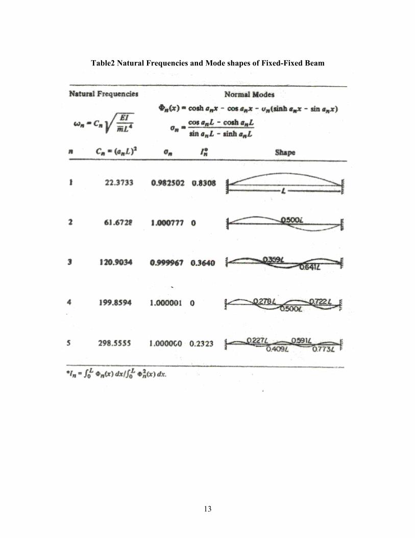
The natural frequencies and mode shapes of simply supported beam, fixed beam and

cantilever beams are shown in table 1, 2 and 3 respectively.

Table1 Natural Frequencies and Mode shapes of Simply supported Beam

13

Table2 Natural Frequencies and Mode shapes of Fixed-Fixed Beam

14

Table3 Natural Frequencies and Mode shapes of Fixed-Free Beam

Orthogonality condition

The most important properties of the normal modes is that of orthogonality. It is this

property which makes possible the uncoupling of the equations of motion. For two

different frequencies ωn ≠ωm, the normal modes must satisfy

( ) ( ) ( ) 0n m

L

m x x x dxφ φ =∫ for n≠m (56)

15

For n=m

2( ) ( )n n

L

m x x dx Mφ =∫ (57)

in which Mn is called the “generalized mass” in the nth mode.

FORCED VIBRATION

Having obtained natural frequencies and mode shapes, the transverse displacement of the

beam can be written as

1

( , ) ( ) ( )i i

i

y x t x tφ η∞

=

=∑ (58)

in which η is the generalized coordinates. Theoretically, infinite number of modes for the continuous systems are possible. However, contribution of higher modes towards the

response is negligible. Hence in computation only first few modes are considered.

Substituting eq.(12) in eq.(2), multiplying both sides by φk , integrating in the domain of the beam and applying orthogonality condition of normal modes, the partial differential

equation of motion can be discretized into uncoupled ordinary differential equation of

motion as 2( ) 2 ( ) ( )i i i i i i it t t Qη ξ ωη ω η+ + =�� � (I=1,2,…) (59)

where Qi is the generalized force whose expression is given by

1( , ) ( )i i

i L

Q f x t x dxM

φ= ∫ (60)

Example: Consider a simply supported beam (uniform cross section) subjected to a

constant force suddenly applied to a section x1 from left support.

Generalized force at x=x1

0 1

0

1( ) ( )

L

i i

i

Q P x x x dxM

δ φ= −∫ (61)

where

2

0

sin ( )2

L

i

i x mLM m dx

L

π= =∫ (62)

Thus 10

2sini

n xQ P

mL L

π=

For the initial condition of zero displacement and zero velocity, the response of

generalized coordinates becomes

16

10

2

2 sin

( ) (1 cos )i n

i

n xP

Lt tmL

π

η ωω

= −

Now using mode superposition technique, the deflection at x at instant t is given by

0

2

2 1( , ) sin (1 cos )sin

2n

n n

P n n xy x t t

mL L

π πω

ω= −∑ (63)

It is apparent that all even the modes do not contribute to the deflection. It is also of

interest to compare the contribution of various modes. This comparison can be done on

the basis of maximum modal displacement disregarding the manner in which these

displacements combine. The amplitude will indicate the relative importance of the

modes. The dynamic load factor (1-cosωnt) has a maximum value of 2 for all the modes. Furthermore, for all modes (except even modes), the modal contribution is simply in

proportion to 1/ω2n. Therefore in higher modes the factor 1/ω2n becomes small and hence

its contribution can be ignored in the superimposition of modes.

MULTISPAN BEAM

Fig.7 Multispan beam

Consider the multispan beam as shown in Fig. 7. With uniform EI , m, c, the equation of

transverse vibration for each span is given by 4 2

4 2( , )

∂ ∂ ∂+ + =

∂ ∂ ∂r r r

b r r

r

y y yEI c m f x t

x t t (64)

rr lx ≤≤0 .,......3,2,1 Nr =

In which the suffix r denotes the rth span; EI, mb and c denotes the flexural rigidity, mass

and viscous damping per unit length respectively. Furthermore, yr is the transverse

deflection on rth span, f(xr,t) is the time-varying external load distribution due to moving

loads, xr is the local co-ordinate along the axis of the rth span at instant t.

The homogeneous solution of the Eqn. (64) ignoring damping is given by

( ) sin cos sinh coshnr nr nr r nr nr r nr nr r nr nr rx A x B x C x D xφ β β β β= + + + (65)

Where Anr, Bnr, Cnr and Dnr are the integration constants, φnr(x) is eigen function of the nth

mode of the rth span. The frequency parameter βnr in the n

th mode is given by

xr

EI, mb

17

24 nr

nr

m

EI

ωβ = (66)

in which ωnr is the natural frequency of the beam (rad/sec). The following boundary

conditions of continuous beam need to be applied:

0),( == tlxy rrr (67)

0),( 1)1( ==++ tlxy rrr (68)

),0(),( 1

)1(

)1(tx

x

ytlx

x

yr

r

r

rr

r

r =∂

∂==

∂

∂+

+

+ (69)

22( 1)

12 2

( 1)

( , ) ( 0, )rr

r r r

r r

yyx l t x t

x x

++

+

∂∂= = =

∂ ∂ 1,2,3...r N= (70)

Using the boundary conditions in Eqn (65), a set of homogeneous equations can be found

in the matrix form as

[ ]{ } { }( ) 0nrV Wβ = (71)

The non-trivial solution of the Eqn. (71) necessitates that the determinant of the matrix

[V(βnr)] should be equal to zero. After expanding the determinant the characteristic polynomial can be solved to find the frequency roots which when substituted in Eqn. (71)

yields the vector {W} and hence the mode shape.

The mode shape function for multi-span continuous beam is given by

sin( )sin( ) sinh( ) 1

sinh( )( )

( ) ( ) 2,3,......

nrnr r nr r

nrnr

r r r r r r

lx x r

lx

PM x Q N x r N

ββ β

βφ

− == + =

(72)

[ ][ ] [ ][ ][ ]( )

cosh( ) cos( ) sin( )sinh( ) sin( ) sinh( )cos( ) sin( )cosh( )

sinh( ) cos( ) cosh( ) sinh( ) sin( )

nr nr nr nr nr nr nr nr nr

r

nr nr nr nr nr

l l l l l l l l lP

l l l l l

β β β β β β β β β

β β β β β

− − −=

− −

[ ][ ] [ ][ ][ ]( )

cos( ) cosh( ) sin( )sinh( ) sinh( ) sinh( )cos( ) sin( )cosh( )

sinh( ) cos( ) cosh( ) sinh( ) sin( )

nr nr nr nr nr nr nr nr nr

r

nr nr nr nr nr

l l l l l l l l lQ

l l l l l

β β β β β β β β β

β β β β β

− + −=

− −

[ ] [ ]{ }( ) cos( ) cosh( ) sinh( ) sinh( ) cosh( ) cos( )r r nr nr nr nr nr nrM x l l x l x xβ β β β β β= − + −

[ ] [ ]{ }( ) cos( ) cosh( ) sin( ) sin( ) cosh( ) cos( )r r nr nr nr nr nr nrN x l l x l x xβ β β β β β= − + −

.

The first five natural frequency parameters for two and three span beams are shown in

Table 4. The length of each span is taken equal.

18

Table 4 First five frequency parameters for multispan beams

Frequency parameters (βnr) Number of

Spans (r) Mode 1 Mode 2 Mode 3 Mode 4 Mode 5

1 π 2π 3π 4π 5π

2 3.1416 3.9272 6.2832 7.0686 9.4248

3 3.1416 3.5500 4.3040 6.2832 6.6920

The natural frequencies ωnr can be found as 2

4( )nr nr

EIl

mlω β=

The mode shapes of continuous beams with two and three equal spans are shown in Fig.8

and Fig.9

Fig.8 First two Mode shapes of continuous beam of two equal spans

Fig.9 First three Mode shapes of continuous beam of two equal spans

19

APPROXIMATE METHODS

The approximate methods are necessary when the exact solution of differential equations

can not be obtained such as in case of non uniform geometry, presence of concentrated

masses and other non classical boundary conditions. Among them Rayeligh-Ritz method

and Gallerkin method are the most popular in the study of continuous system. The

success of these two methods depends on the choice of shape function that need to satisfy

the geometrical boundary conditions. In this lecture, Rayeligh-Ritz method and Gallerkin

methods will be decribed.

Rayeligh-Ritz method

Let Umax and Tmax be the potential and kinetic energy of the system undergoing simple

harmonic motion in free vibration.

Then

max

max2

T

U=ω (73)

Let the shape function be

)(....)()()( 2211 xCxCxCxw nnφφφ +++= (74)

where Ci are the constants and φI(x) are the admissible functions satisfying the boundary conditions. The maximum K.E and P. E are expressed as

ji

i j

ij CCkU ∑∑=2

1 and ji

i j

ij CCmT ∑∑=2

1 (75)

kij and mij depends on the type of problem. For example, for the beam we have

dxEIk jiij ∫ ′′″= φφ and dxmm jiij ∫= φφ (76)

where as for longitudinal vibration of bars

dxEAk jiij ∫ ′′″= φφ and dxmm jiij ∫= φφ (77)

We now minimize ω2 by differentiating it with respect to each of the constants. Thus

02

max

maxmax

maxmax2

=∂

∂−

∂

∂

=∂∂

T

C

TU

C

UT

C

ii

i

ω (78)

which is satisfied by

0max

max

maxmax =∂

∂−

∂

∂

ii C

T

T

U

C

U (79)

20

Using eq.(73), we have

0max2max =∂

∂−

∂

∂

ii C

T

C

Uω (80)

The two terms of the equations are then

∑=∂

∂

j

jij

i

CkC

Umax and ∑=∂

∂

j

jij

i

CmC

Tmax (81)

and so finally we get

0)(...)()( 2

2

2

221

2

11 =−++−+− ininniiii mkCmkCmkC ωωω (82)

With i varying from 1 to n there will be n such equations, which can be arranged in

matrix form

( ){ } 0][][ 2 =− CMK ω (83)

For non-trivial solution, the determinant of the matrix is equated to zero and

characteristic polynomial can be obtained. The solution gives n natural frequencies and

corresponding to each natural frequency, the {C} is found to obtain the mode shape

function.

Gallerkin Method

In this method, we need to know the governing differential equations of the continuous

system. Again, the shape function is chosen such that it satisfies the geometric boundary

conditions.

Consider the eigen value problem

][][ wMwL λ= (84)

Here L and M are self adjoint homogeneous differential operators of order 2p and 2q. The

function w can be taken in the form series of n comparison function as stated in the

previous method. Substituting, the series of comparison functions in the differential

equations, an error will be obtained.

][][*

wMwL n λε −= (85)

where λ* is the corresponding estimate of the eigenvalue λ. Considering the orthogonality of the error with the assumed functions, Gallerkin’s equation is obtained as

0=∫ dDD

kεφ , k=1,2,..,n (86)

The following relations are obtained

j

n

j

ij

D

j

n

i

i

D

ni CKdDLCdDwL ∑∫∑∫==

==11

][][ φφ (87)

21

and similarly j

n

j

ij

D

ni CmdDwM ∑∫=

==1

][φ (88)

Which leads to

0)( *

1

=−∑=

jij

n

j

ij CmK λ , I=1, 2,…,n (89)

Expansion of the eq.(89) results a similar matrix equation as in eq.(83), which can be

solved as stated before.

CLOSURE

The basic dynamics of continuous system has been discussed. The inertia and stiffness

and damping are distributed along the domain. The solution of free vibration problem

leading to natural frequencies and mode shapes are outlined by exact method and by

approximate method. The forced vibration problem is also discussed with the help of

mode superposition of method. Torsional and Axial vibrations of bars (represented by

second order partial differential equations ) and bending vibrations of beam (represented

by fourth order partial differential equations) are illustrated with some examples.

Further Reading

1. M. Paz, “Structural Dynamics”, CRC publishers, 1987

2. L. Meirovitch, “Elements of Vibration Analysis”, Mc Graw Hill Co., 1986

3. L. Meirovitch, “Analytical Methods in Vibrations”, Macmillan Co., 1967

4. D. J. Gorman, “Free Vibration Analysis for beams and shafts”, John Willey and

Sons, 1975

5. W. T. Thompson, “Theory of Vibrations with Applications”, CBS, 1988

6. I. A. Karnovsky and O. I. Lebed, “Formulas for Structural Dynamics”, Mc Graw,

2000