Munich Personal RePEc Archive

Standards of living and health status:

the socioeconomic determinants of life

expectancy gain in sub-Saharan Africa

Keita, Moussa

June 2013

Online at https://mpra.ub.uni-muenchen.de/57553/

MPRA Paper No. 57553, posted 25 Jul 2014 17:54 UTC

1

Standards of living and health status: the socioeconomic determinants

of life expectancy gain in sub-Saharan Africa

Moussa Keita

PhD Student at CERDI *

(June 2013)

Abstract

Using a panel dataset on 45 sub-Saharan Africa countries (SSA), this study analyzes empirically

the socioeconomic determinants of life expectancy gain (considered as an indicator of global

health improvement at country level). In order to treat heterogeneity and endogeneity concerns,

we use multiple estimation methods including pooling, fixed-effect, long difference and system

GMM. Our analyses show that income is critical for health enhancement. Particularly, we find

that GDP per capita is strongly and positively correlated with life expectancy gain. Furthermore,

variables such as adult literacy, access to improved sanitation and safe water appear positively

correlated health gain. In contrast the high incidence of extreme poverty is negatively correlated

with heath gain while the impact of income inequality seems ambiguous.

Codes JEL: C12, C51, I11, I12 Key words: Standards of living, health, life expectancy at birth. Contact Info Email : keitam09@ymail.com

*Centre d’Etudes et de Recherches sur le Développement International, France I would like to thank to my thesis supervisors Catherine Araujo-Bonjean and Martine Audibert for their comments, criticisms and suggestions. I also thank Fousseni Traoré, Researcher at International Food Policy Research Institute (IFPRI) for his reading and precious comments.

2

1. Introduction

Since the second half of the last century, the life expectancy1 has significantly increased in most

of the developing countries, in particular, in Sub-Saharan Africa (SSA) where it went from 40.4

years in 1960 to 54.16 years in 2010 (World Bank, 2010). As the debate has long existed about

the causes of the mortality decline, many studies that investigate some possible explanations

concerning the levels and the variation of life expectancy show mixed results. Various answers

were given to the question of what factors has been most associated with the increases in levels

of life expectancy. For some authors, this has been the result of the success in the application

of communicable disease control technologies through public health activities (Stolnitz, 1975).

And for others, it has been mainly attributable to the global improvement in the economic

situation, particularly the elimination of famines and improved nutrition available to the people

of the less developed countries (Krishnan, 1975).

Despite these divergent views, these studies do not ignore the role that has been played by the

conjunction of various socio-economic factors which resulted in an overall decrease in mortality

risk over time. The improvement of health status observed in developing countries may have

been also driven by the concomitant rises in economic levels, social well-being and health

service investments through the increase in per capita income combined with higher health

expenditure and progress in medical technologies. In this study, our analysis is focused

essentially on those factors directly linked to the population living conditions such as income,

poverty, inequality, education, social and environmental factors.

Regarding number of studies carried out on the health problematic in developing countries, our

study can be considered as an update of some of them although we take a different

methodological step. In fact, authors like Kabir (2008) which examines the socio-economic

determinants of life expectancy for 91 developing countries, uses probit regressions to

determine the probability for a country to be in one of the following countries groups: low,

medium and high life expectancy. As many of his explanatory variables turned out to be

1 Life expectancy at birth expresses the average length of time that an individual born in a given period would live

if he experienced the mortality rates of that period throughout his lifetime. It indicates the number of years a newborn infant would live if prevailing patterns of mortality at the time of its birth is considered the same throughout its life. Life expectancy at birth provides a useful snapshot of mortality and represents a more synthetic measure of health status that is comparable across populations and time. In quantifying health status, life expectancy is, as for mortality rate, one of the most used traditional measures of global health. Although, recently other health indicators have been developed to represent not only death or living but also the condition of health. These indicators include the Disability Adjusted Life Year (DALY) and the Disability Adjusted Life Expectancy (DALE). But, these last indicators remain, in some respects, rarely used by researchers in large scales cross-country studies, given their very detailed data requirement.

3

statistically insignificant in most of his regressions, the author deduce that the relevant socio-

economic factors like per capita income, education, health expenditure, access to safe water,

and urbanization cannot always be considered to be influential in determining life expectancy

in developing countries. Also, Fayissa and Gutema (2005) estimate a health production function

for Sub-Saharan Africa based on the Grossman (1972) theoretical model that treats social,

economic, and environmental factors as inputs of health production function. Socioeconomic

and environmental factors such as income per capita, illiteracy rate, food availability, ratio of

health expenditure to GDP, urbanization rate, and carbon dioxide emission per worker are

specified as determinants of health status. The model is estimated by one-way and two-way

panel data approaches. Their results suggest that an increase respectively in income per capita,

food availability and literacy rate are well associated with improvement in life expectancy.

These results lead authors to suggest that health policy that focus solely on provision of program

excluding socioeconomic aspects, may do little toward improving the current health status.

But, the main criticism that could be addressed to these two previous studies is that, for the first,

it does not exploits the temporal dimension allowing him to control for countries specificities

by the use of panel methods. For the second study, the endogeneity issue of GDP per capita is

not addressed. Hence, the accuracy of the estimations is seriously compromised.

In this study, we use alternative approach to control potential estimation bias by exploiting both

the temporal dimension and dealing with the endogeneity problem. Our dataset is a panel of 45

countries which coverage span the period 1960-20112. For each variable, we have averaged

over a five-year period the annual data to reduce annual fluctuations and measurement errors.

The work is organized as follow. In Section 2, we proceed to the literature on recent empirical

studies focusing on the determinants of health status particularly in developing countries. The

third section is devoted to the presentation of data and descriptive statistics. In the fourth

section, we develop the econometric model by proposing multiples estimation methods. This

section is then accompanied by a fifth one in which we conduct diagnostic tests to assess the

quality of our estimation methods. In the sixth section, we proceed to the presentation and the

discussion of the estimation results followed by a general conclusion.

2 The list of the countries in the sample is presented in appendix.

4

2. Literature Review

Country wealth is one of the most discussed health causal factor in the literature. It has long

been evidenced a strong relation between health and the absolute level of income (measured by

per capita GDP). It’s established that the lower per capita GDP, the lower life expectancy

(World Bank, 1993). However, once countries attain some threshold level of income, the

correlation between income and life expectancy become weak. Hence increases in per capita

GDP no longer appear to be associated with life expectancy gains (Wilkinson, 1996). This

author found that health of a population is directly related to its average income and no

consistent relation is above that level. Rogers (1979) which provided a conceptual framework

of the relation between income and life expectancy based on the observations from developed

countries found that the relation is non-linear. He observed that life expectancy rises at a

declining rate as income grows. Education is also considered as one major influential

determinant of life expectancy. Many studies have empirically demonstrated the dominant role

of education in explaining the differences in health status. They highlight that life expectancy

differs considerably in relation to education (Grabauskas and Kalediene, 2002; Kalediene and

Petrauskiene, 2000). But in general, few measures of education variables still be employed in

the analyses of health status determinants. For example, Rogot et al (1992) revealed that life

expectancy varies directly with years of schooling while Gulis (2000) which uses literacy rate

shows statistically significant role of this variable in explaining life expectancy.

Access to health care is considered as the most direct way of improving health status essentially

through curative and preventive treatments including the provision of medical goods and

facilities such as clean water, nutrition, mosquito (Gertler and van der Gaag, 1990). In a

multivariate linear regression analysis on data of 156 countries, Gulis (2000) found that, access

to safe drinking water impacts significantly life expectancy. However, the most used variables

to test the effects of health inputs are typically the health resources indicators. These resources

include health expenditure, health workforce (physician, nurse, etc.) and health infrastructure

(hospital, and hospital beds, etc). The total health expenditure is perceived to have significant

influence on life expectancy because it directly helps reduce mortality and morbidity (Kabir,

2008). Using cross-country time series data, Hitiris and Posnet (1992) find negative correlation

between health spending and mortality rates. Grubaugh and Santerre (1994) find positive and

significant impact of number of doctors and number hospital beds on infant mortality rates.

5

In addition to the previously determinants, other general characteristics of the population are

considered among health determinants. Gender is one of these components. There is well-

known evidence that females live longer than males. Population behavior is another factor that

affects heath status; for example, smoking, alcohol consumption, and daily activity. Phelps

(1997) argued that the role of medical care is considerably small relative to the lifestyle.

Urbanization also plays a crucial role in determining life expectancy. Although, Rogers and

Wofford (1989) revealed that urbanization was less influential on life expectancy than

anticipated, urban inhabitants of the developing countries generally enjoy improved medical

care and means of life, better education, and other improved socio-economic facilities, which

impact positively on health outcomes.

Regarding the particular specificities of Sub-Saharan Africa region, we notice that the

population of this region has been living under serious life-threatening diseases (malaria,

diarrhoeal diseases, respiratory infections, AIDS, etc.), which have important implications for

reduction in life expectancy. The SSA region also suffers from violent conflicts. Davis and

Kuritsky (1997) found that, in countries experiencing severe conflicts, life expectancy has been

shortened by an average 2.35 years. Since these geographical specificities tend to show an

unfavorable context in SSA, it may be important to include in the analysis some of the aspects

related to country epidemiologic and socioeconomic environment.

3. Data and Sources

3.1. Sample

The sample used in this study consists of 45 of the 47 SSA countries reported by the World

Bank3 for which sufficient data are available over long period both for the life expectancy

variable and the other interest variables. All the variables are extracted from the World

Development Indicators database from which we compile a panel dataset covering the period

1960-2011. The choice of 1960 as the base year is guided, in particular, by the idea that 1960

is, for many SSA countries, a reference year marking their independence. Thus one may think

that the observed evolution in life expectancy since this date can be considered as a good

indicator of the progress realized by these countries in terms of health improvement.

3 http://go.worldbank.org/JRVQH9W970

6

3.2. Evolution of Life expectancy in SSA

Since the second half of the last century, it has been observed a significant increase in life

expectancy in the world. According to WPP (2010)4, over the five year-period 1950-1955, the

average life expectancy at the world level was 48 years and it had reached 68 years by 2005-

2010. In 1950-55, the more developed regions already had a high expectation of life (66 years)

and have since experienced further gains in longevity (76.9 years), 11 years higher than in the

less developed regions where the expectation of life at birth is 65.9 years in 2005-10.

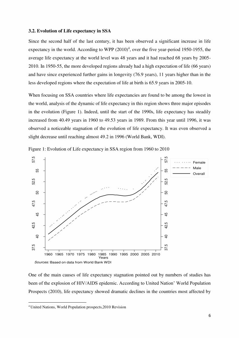
When focusing on SSA countries where life expectancies are found to be among the lowest in

the world, analysis of the dynamic of life expectancy in this region shows three major episodes

in the evolution (Figure 1). Indeed, until the start of the 1990s, life expectancy has steadily

increased from 40.49 years in 1960 to 49.53 years in 1989. From this year until 1996, it was

observed a noticeable stagnation of the evolution of life expectancy. It was even observed a

slight decrease until reaching almost 49.2 in 1996 (World Bank, WDI).

Figure 1: Evolution of Life expectancy in SSA region from 1960 to 2010

One of the main causes of life expectancy stagnation pointed out by numbers of studies has

been of the explosion of HIV/AIDS epidemic. According to United Nation’ World Population

Prospects (2010), life expectancy showed dramatic declines in the countries most affected by

4 United Nations, World Population prospects,2010 Revision

37.

54

04

2.5

45

47.

55

05

2.5

55

57.

5

37.

54

04

2.5

45

47.

55

05

2.5

55

57.

5

1960 1965 1970 1975 1980 1985 1990 1995 2000 2005 2010Years

Female

Male

Overall

Sources: Based on data from World Bank WDI

7

HIV/AIDS. In Botswana, for example, where HIV prevalence was estimated at 24.8 percent in

2009 (among the aged 15-49 years), life expectancy has fallen from 64 years in 1985-90 to 49

years in 2000-05. And for Southern Africa as a whole, where most of the worst affected

countries are, life expectancy has fallen from 61 to 51 years over the last 20 years. In addition

to impact due to the AIDS epidemic, other factors have been identified as having contributed

to the stagnation of life expectancy. These factors include armed conflict, economic stagnation,

and resurgent infectious diseases such as tuberculosis and malaria.

However, despite this significant stagnation, one can observe again, from the second half of

1990, an increase of life expectancy which has reached 54.16 years in 2010. This recovery was

mainly driven in part by the reduction of the magnitude of AIDS virus propagation in many

countries, also due to the roles played by public health policies, which, for the most, are part of

the MDG launched since the early 2000s.

On gender aspects, it is widely recognized that female life expectancy at birth is higher than

that of males in nearly all countries around the world. According to WPP (2010), females have

a life expectancy of 70 years, compared to 66 years for males in 2010. The female advantage

in the more developed regions is around 7 years while in the less developed regions, it’s almost

3.5 years.

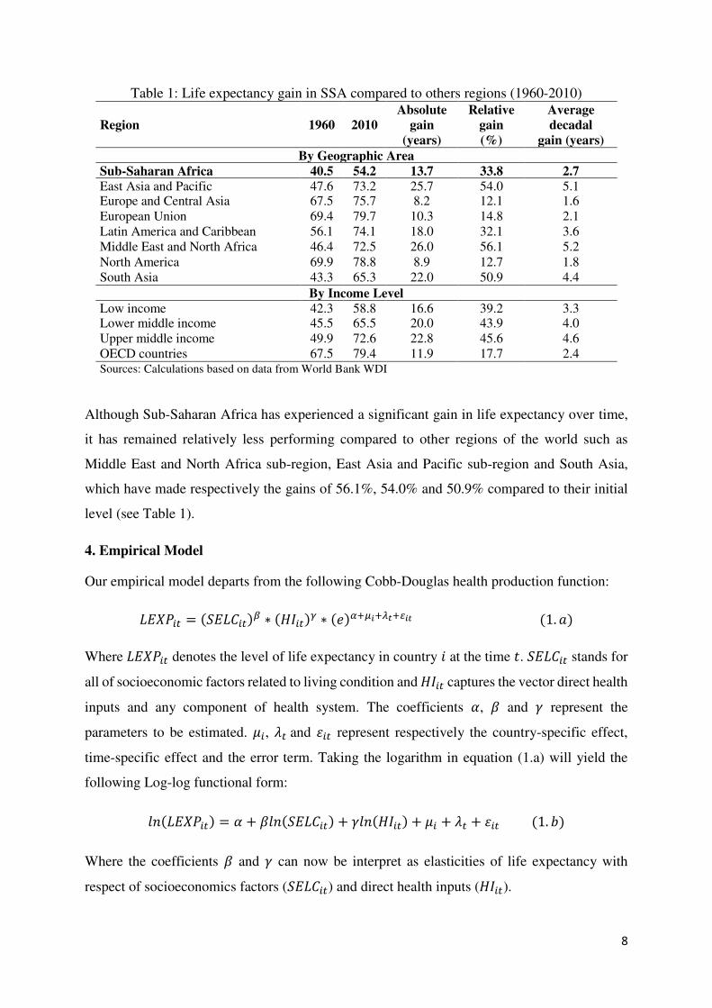
In terms of longevity gain in Sub-Saharan Africa, despite non-monotonic evolution of life

expectancy, the region has still made significant progress in terms of improvement in health

status. Over the period 1960-2010, it recorded an absolute gain of 14 years (an increase of life

expectancy of 33.8 percent compared to 1960 level). This represents an average of 2.7 years of

longevity gain every 10 years (see table 1).

8

Table 1: Life expectancy gain in SSA compared to others regions (1960-2010)

Region 1960 2010

Absolute

gain

(years)

Relative

gain

(%)

Average

decadal

gain (years)

By Geographic Area

Sub-Saharan Africa 40.5 54.2 13.7 33.8 2.7

East Asia and Pacific 47.6 73.2 25.7 54.0 5.1 Europe and Central Asia 67.5 75.7 8.2 12.1 1.6 European Union 69.4 79.7 10.3 14.8 2.1 Latin America and Caribbean 56.1 74.1 18.0 32.1 3.6 Middle East and North Africa 46.4 72.5 26.0 56.1 5.2 North America 69.9 78.8 8.9 12.7 1.8 South Asia 43.3 65.3 22.0 50.9 4.4

By Income Level

Low income 42.3 58.8 16.6 39.2 3.3 Lower middle income 45.5 65.5 20.0 43.9 4.0 Upper middle income 49.9 72.6 22.8 45.6 4.6 OECD countries 67.5 79.4 11.9 17.7 2.4 Sources: Calculations based on data from World Bank WDI

Although Sub-Saharan Africa has experienced a significant gain in life expectancy over time,

it has remained relatively less performing compared to other regions of the world such as

Middle East and North Africa sub-region, East Asia and Pacific sub-region and South Asia,

which have made respectively the gains of 56.1%, 54.0% and 50.9% compared to their initial

level (see Table 1).

4. Empirical Model

Our empirical model departs from the following Cobb-Douglas health production function: 𝐿𝐸𝑋𝑃𝑖𝑡 = (𝑆𝐸𝐿𝐶𝑖𝑡)𝛽 ∗ (𝐻𝐼𝑖𝑡)𝛾 ∗ (𝑒)𝛼+𝜇𝑖+𝜆𝑡+𝜀𝑖𝑡 (1. 𝑎)

Where 𝐿𝐸𝑋𝑃𝑖𝑡 denotes the level of life expectancy in country 𝑖 at the time 𝑡. 𝑆𝐸𝐿𝐶𝑖𝑡 stands for

all of socioeconomic factors related to living condition and 𝐻𝐼𝑖𝑡 captures the vector direct health

inputs and any component of health system. The coefficients 𝛼, 𝛽 and 𝛾 represent the

parameters to be estimated. 𝜇𝑖, 𝜆𝑡 and 𝜀𝑖𝑡 represent respectively the country-specific effect,

time-specific effect and the error term. Taking the logarithm in equation (1.a) will yield the

following Log-log functional form: 𝑙𝑛(𝐿𝐸𝑋𝑃𝑖𝑡) = 𝛼 + 𝛽𝑙𝑛(𝑆𝐸𝐿𝐶𝑖𝑡) + 𝛾𝑙𝑛(𝐻𝐼𝑖𝑡) + 𝜇𝑖 + 𝜆𝑡 + 𝜀𝑖𝑡 (1. 𝑏)

Where the coefficients 𝛽 and 𝛾 can now be interpret as elasticities of life expectancy with

respect of socioeconomics factors (𝑆𝐸𝐿𝐶𝑖𝑡) and direct health inputs (𝐻𝐼𝑖𝑡).

9

The variables incorporated in the analysis are the per capita GDP in purchasing power parity

(PPP) dollar representing the per capita income. Although the per capita health expenditure is

recognized as one of the key variable of health inputs, we have not included it in the regressions

because of the acute problem of collinearity with income. Nevertheless, we used the share of

public health spending in total health expenditures. Since the major part of the health

expenditures are endorsed by the government in developing countries, this indicator,

representing, in fact, the public effort in health production, could serve to measure the impact

and the effectiveness public spending on life expectancy. Still based on literature, we have also

included the adult literacy, fertility rate, access to safe water and sanitation, number of

physicians per thousand people. We control for country epidemiologic environment such as the

prevalence of HIV (percentage of people living with HIV) and we also include variables related

to socioeconomic environment such as incidence of extreme poverty (poverty headcount ratio

at $1.25 PPP a day in % of population) and level of inequality represented by the gini index.

4. Estimation Strategy

4.1. Pooling and Fixed Effect Estimations

Using equation (1.b), we first adopt the pooled cross-sectional regression model as our basic

specification. In this estimation, all the individual observations on country and time period are

pooled using five-year period average for life expectancy and explanatory variables. Assuming

that the error term 𝜀 is stochastic and normally distributed with mean zero and constant

variance, we first estimate equation (1.b) by Ordinary Least Squares (OLS). In this pooling

estimation, one could control for country specific effect by including dummy variable for each

country. But, given the high number of countries (45), introducing dummies variable would

lead to a dummy variable trap, so we chose to control only for the time-effect by introducing

time dummies which capture effects associated five-year periods we have constituted. The

results obtained from this first estimation are presented in column 1 of Table 2.

Although this OLS estimator remains unbiased and consistent if the error term does not contain

any components that are correlated with explanatory, it may suffers from endogeneity problem

of some explanatory variables. For instance, as there may be a strong reverse causality between

health status and income, this will arise to the endogeneity problem that must be corrected using

instrumental variable procedure. For that, we instrument GDP per capita following Pritchett

and summers (1996). These authors, using results from Levine and Renelt (1992) and Easterly

et al. (1993), used as instruments the terms-of-trade shocks and the ratio of investment to GDP.

10

Levine and Renelt (1992) showed that the ratio of investment to GDP is robustly related to

growth. Easterly, Kremer, Pritchett, and summers (1993) have shown that the growth rates of

income over five-year periods are explained in part by terms-of-trade shocks. This finding

suggests us to use terms of trade shocks5 as an instrument, since the five-year changes in terms

of trade are convincingly exogenous, both in the sense of not having a direct relation to

health and not being determined by any other country-level variable that jointly affect

income growth rates (Pritchett and Summers,1996). Smith and Haddad (1999) also suggest

the use of country economic openness as potential candidate for income instrumentation, as

economic openness may improve national income but not otherwise directly affect health.

Therefore, in complement of terms-of-trade shocks and ratio of investment to GDP, we use

country openness measured as the ratio of trade volume (sum of imports and exports) to GDP.

Results obtained from the 2SLS pooling estimations are presented in column 2 of Table 2.

Trying to control for countries specific effects, we estimate fixed-effects model (Baltaji, 1995)

which allows us to captures country-specific unobservables that may affect life expectancy and

which do not vary over time. Time-invariant factors may be climatic conditions, countries’

physical environments and deeply-embedded cultural and social norms which can be controlled

by 𝜇𝑖 in the estimations. The fixed-effects approach, in addition to removing bias, can serve to

control for measurement errors and non comparabilities in the data due to definitional and

measurement differences at the country level (Ravallion and Chen 1996). Hence, in addition to

previous time dummies (capturing time-specific effect), we introduce a single time-trend

variable which can capture the long run effects of time such as those related to technological

progress and innovations in medicine. The model is then estimated par the within approach

whose results are summarized in column 3 and 4 of Table 2.

5 The terms of trade index measures the relative prices of a country's exports and imports. We use Net barter terms of trade index as term of trade indicator calculated as the percentage ratio of the export unit value indexes to the import unit value indexes (World Bank, WDI).. For each country, we estimate a deterministic trend, which is then extracted from the original series to get the cycle. This cyclical component (considered a deviation of the series compared to long-run equilibrium) is retained as our shock indicator since it’s highly affected by regular shocks (Perron, 1989).

11

Table 2: Pooling and fixed-effects estimations results POOLED WITHIN VARIABLES OLS 2SLS OLS 2SLS

Gdp_pcapita 2.3e-06** 1.8e-05*** 1.2e-06** 3.7e-07

(0.021) (0.000) (0.037) (0.812)

Share_Public_health_expenditure 0.008** 0.010** 0.018*** 0.019***

(0.030) (0.036) (0.006) (0.007)

Sanitary_access_rate 0.026*** 0.057* 0.015* -0.017

(0.003) (0.063) (0.090) (0.121)

Safe_water_access_rate 0.070*** 0.134*** 0.047** 0.019**

(8.3e-04) (1.7e-04) (0.042) (0.047)

Adult_literacy_rate 0.031** 0.022** 0.0018* 3.1e-05*

(0.048) (0.030) (0.089) (0.099)

Fertility_rate 0.026 0.153** -0.229*** -0.243***

(0.541) (0.0353) (4.7e-05) (2.1e-04)

Urbanization _rate -0.015 -0.027** 0.051 0.089

(0.106) (0.0458) (0.143) (0.139)

Physician_per_1000inhabt 0.012*** 0.007** 0.007** 0.003**

(0.001) (0.020) (0.028) (0.039)

Prevalence_HIV -0.015*** -0.013** -0.014*** -0.008*

(1.3e-04) (0.0298) (3.6e-04) (0.058)

Extreme_Poverty_headcount_ratio -0.079*** -0.074*** -0.050*** -0.041***

(0.001) (1.9e-07) (1.7e-06) (2.0e-04)

Gini_index 0.091 0.139* 0.059 0.027

(0.130) (0.0975) (0.213) (0.590)

Constant 3.972*** 3.333*** 3.450*** 3.485***

(8.1e-04) (6.9e-04) (2.3e-04) (8.1e-03)

Time_trend no no yes yes

Time dummies yes yes yes yes

Sub-regions dummies yes yes yes yes

Observations 271 271 271 225 R-squared 0.718 0.432 0.547 0.539

Prob F test that all u_i=0 0.000 0.000 Prob Wald test corr( u_i, Xb)=0 0.000 0.000

Pvalue in parentheses *** p<0.01, ** p<0.05, * p<0.1 Sample: 1980-2010, Cf. section 5 for first stage regressions results

4.3. Long-Difference Estimation

As the annual or five-year change in life expectancy is very low, it seems more interesting to

examine its evolution over a relatively long period in order to be able to identify the factors that

can significantly contribute to the long-term variation. The aim of the long-difference

estimation is to exploit the long-run changes in health status with respect to long-run changes

in explanatory variables. In this approach, one suppose that the full effect of some of the

explanatory variables can go beyond the just yearly or five-years changes in life expectancy.

For example, health expenditure which is realized in a given year will continues to have effects

12

even in the subsequent years. In that case, rather than only associate expenditures with the

corresponding life expectancy, one could analyze changes in life expectancy over a given period

in relation to the absolute change in the interest variable over the same period. Thus, we estimate

equation (1.b) in long differences (LD) approach following Acemoglu and Johnson (2005).

The LD approaches make interpretation easier as they directly measure the effect of change in

economic variables between two dates on the change in life expectancy between the same dates.

This approach may be useful because it is less vulnerable to serial correlation problems in the

error terms (Acemoglu and Johnson, 2005). This method may be just limited to two dates panel.

For examples, the difference observed between 1980 and 1989, between 1990 and 2000 or

between 2000 and 2010. Since we consider only two dates, this estimation procedure is

equivalent to the first-differenced specification. Hence using equation (1.b), one can write the

LD specification as follows: ∆𝑡0𝑡1𝑙𝑛(𝐿𝐸𝑋𝑃𝑖𝑡) = 𝛽∆𝑡0𝑡1𝑙𝑛(𝑆𝐸𝐿𝐶𝑖𝑡) + 𝛾∆𝑡0𝑡1𝑙𝑛(𝐻𝐼𝑖𝑡) + ∆𝑡0𝑡1𝜆𝑡 + ∆𝑡0𝑡1𝜀𝑖𝑡 (2. 𝑎)

Where ∆𝑡0𝑡1𝑙𝑛(𝐿𝐸𝑋𝑃𝑖𝑡) denotes the life expectancy gain in country 𝑖 determined as the absolute

variation of the level of life expectancy between the two dates 𝑡0 and 𝑡1. ∆𝑡0𝑡1𝑙𝑛(𝑆𝐸𝐿𝐶𝑖𝑡) is

the variation all of socioeconomic factors over the same period and ∆𝑡0𝑡1𝑙𝑛(𝐻𝐼𝑖𝑡) the variation

of the direct health inputs and others health system components. ∆𝑡0𝑡1𝜆𝑡 and ∆𝑡0𝑡1𝜀𝑖𝑡 represent

respectively, time-varying factors and the error term. Note that in this specification, the country-

specific effect and the intercept term are just eliminated by the difference operator ∆ since these

factors are supposed to be constants over time. But this is not necessarily the case for time-

specific since ∆𝑡0𝑡1𝜆𝑡 can be different from zero. To control for this issue, we introduce the

constant term in the difference equation6. The coefficient 𝛽 and 𝛾 represent the parameters to

be estimated.

Applying the difference operator on the logarithm elements, equation (2.a) can be rearranged

and rewritten in terms of relative variation. Thus, we obtain the following equation (2.b):

𝑙𝑛 (𝐿𝐸𝑋𝑃𝑖𝑡1𝐿𝐸𝑋𝑃𝑖𝑡0 ) = 𝛽𝑙𝑛 (𝑆𝐸𝐿𝐶𝑖𝑡1𝑆𝐸𝐿𝐶𝑖𝑡0) + 𝛾𝑙𝑛 (𝐻𝐼𝑖𝑡1𝐻𝐼𝑖𝑡0) + ∆𝑡0𝑡1𝜆𝑡 + ∆𝑡0𝑡1𝜀𝑖𝑡 (2. 𝑏)

6 As the constant is initially absent in this equation, introducing this variable will allows to capture the difference in the

coefficients of the times dummies. This is easily mathematically demonstrable that this will be equivalent to ∆𝑡0𝑡1𝜆𝑡.

13

This equation is then estimated by 2SLS over three sub-periods and over the entire period.

Table3 presents the results from these estimations.

Table 3: Variation of Life expectancy FIRST-DIFFERENCE 2SLS

VARIABLES (1980-1989) (1990-1999) (2000-2010) (1980-2010)

Gdp_pcapita

-7.2e-06 2.4e-05** -2.3e-06 9.1e-06*

(0.149) (0.043) (0.183) (0.083)

Share_Public_health_expenditure

0.126** 0.010** 2.2e-05* 0.068***

(0.046) (0.017) (0.099) (0.005)

Sanitary_access_rate

1.330** -0.012 0.021 0.098**

(0.026) (0.596) (0.361) (0.016)

Safe_water_access_rate

2.771 -0.027 0.040* 0.148***

(0.117) (0.547) (0.058) (0.003)

Adult_literacy_rate

-0.005 0.004* 0.018** 0.117**

(0.673) (0.078) (0.037) (0.011)

Fertility_rate

0.314*** -0.321** -0.095** -0.170**

(9.2e-04) (0.028) (0.044) (0.018)

Urbanization _rate

-0.025 0.090** 0.037 -6.4e-05*

(0.101) (0.018) (0.338) (0.099)

Physician_per_1000inhabt

6.3e-04 0.012*** 0.004* 0.012**

(0.886) (0.002) (0.060) (0.034)

Prevalence_HIV

---

---

-0.011** -0.004* -0.055***

---

(0.030) (0.098) (3.8e-08)

Extreme_Poverty_headcount_ratio

-0.003 -0.027** 0.004 -0.060**

(0.637) (0.018) (0.817) (0.012)

Gini_index -0.010* 0.056** -0.028 0.117**

(0.082) (0.045) (0.536) (0.029)

Constant for ∆𝑡0𝑡1𝜆𝑡 0.010*** -0.011** 0.038*** 0.022**

(2.0e-06) (0.039) (6.8e-07) (0.049)

Sub-regions dummies yes yes yes yes

Observations 45 45 45 45 R-squared 0.786 0.565 0.589 0.722

Pvalue in parentheses *** p<0.01, ** p<0.05, * p<0.1 As Prevalence_HIV=0 for all countries between 1980-1989, thus this variable is dropped from regressions for this period7.

4.4. Dynamic Specification

We also attempt to explore dynamic aspect of life expectancy by using standard dynamic

models including lagged dependent variable as a regressor. The dynamic specification is a way

to overcome the weakness of the previous methods. Its specification is expressed as follow:

7 All the estimations previously done were made by assigning zero HIV prevalence over 1980-1989 for all countries since no HIV prevalence is observed during that period. And the HIV prevalence is rescaled using (+10-05) in logarithmic form.

14

𝑙𝑛(𝐿𝐸𝑋𝑃𝑖𝑡) = 𝛼 + 𝛿𝑙𝑛(𝐿𝐸𝑋𝑃𝑖𝑡−1) + 𝛽𝑙𝑛(𝑆𝐸𝐿𝐶𝑖𝑡) + 𝛾𝑙𝑛(𝐻𝐼𝑖𝑡) + 𝜇𝑖 + 𝜆𝑡 + 𝜀𝑖𝑡 (3. 𝑎)

Where 𝑙𝑛(𝐿𝐸𝑋𝑃𝑖𝑡) and 𝑙𝑛(𝐿𝐸𝑋𝑃𝑖𝑡−1) are respectively the log of life expectancy at periods 𝑡

and 𝑡 − 1. 𝑆𝐸𝐿𝐶𝑖𝑡 and 𝐻𝐼𝑖𝑡 are the other regressors. 𝜇𝑖, 𝜆𝑡 and 𝜀𝑖𝑡 represent respectively the

country-specific effects, time-specific effects and the error term. If 𝛿 ≠ 0, thus 𝑙𝑛(𝐿𝐸𝑋𝑃𝑖𝑡)

will be function of error term, and OLS estimation will be biased and inconsistent. Eliminating

this bias requires, first, undertaking the short first-difference transformation to wipe out the

country fixed-effect term. This yields the following estimating equation: ∆𝑙𝑛(𝐿𝐸𝑋𝑃𝑖𝑡) = 𝛿𝑙𝑛(∆𝐿𝐸𝑋𝑃𝑖𝑡−1) + 𝛽𝑙𝑛(∆𝑆𝐸𝐿𝐶𝑖𝑡) + 𝛾𝑙𝑛(∆𝐻𝐼𝑖𝑡) + ∆𝜆𝑡 + ∆𝜀𝑖𝑡 (3. 𝑏)

To implement this estimation, we use a system of moment equations in system GMM approach

(Blundell and Bond, 1998) in which we have two block of a stacked data organized in the form

of system. The first block is built out of the data in level (equation 3.a) and the second of data

in differences (equation 3.b). In this system, lagged variables in levels serve to instrument the

differenced variables and lagged differences to instrument variable in levels.

In panel data with a large number of cross-sections and a small number of time periods, the

system GMM estimator has much smaller finite sample bias and is much more accurate in

estimating autoregressive parameters. But one caveat of system GMM is that including

excessive number of instruments dilutes the power of Hansen’s overidentification test and the

test may falsely reject the null hypothesis that the instruments are valid8.

In estimation, lagged life expectancy and per capita income are variables that are treated as

endogenous and all of the estimations are performed by the two-step GMM. We check

robustness of the model by using different time lags by changing the number of instruments in

the system estimation. The results from this estimations are presented in Table 4.

8 See Roodman (2008) for a discussion on the different problems which can arise by using too many instruments.

15

Table 4: Dynamic estimation results: GMM estimation

VARIABLES Coeff P.values

Lag_ Life_expect 0.600*** (8.6e-07)

Gdp_pcapita 1.1e-06** (0.015)

Share_Public_health_expenditure 0.015*** (0.002)

Sanitary_access_rate 0.014*** (0.008)

Safe_water_access_rate 0.019** (0.026)

Adult_literacy_rate 0.010** (0.027)

Fertility_rate -2.3e-04 (0.996)

Urbanization _rate 0.016 (0.121)

Physician_per_1000inhabt 0.006** (0.017)

Prevalence_HIV -0.009** (0.030)

Extreme_Poverty_headcount_ratio -0.029* (0.074)

Gini_index -0.008 (0.849)

Constant 1.749*** (0.001)

Time_trend yes ---

Time dummies yes ---

Sub-regions dummies yes --- Observations 225 --- Number of instruments 38 --- Sargan test of overid.(Not robust, but not weakened by many instruments) Prob > chi2 = 0.033 Hansen test of overid(Robust, but weakened by many instruments.) Prob >chi2 = 0.096 Arellano-Bond test for AR(1) in first differences; H0:no serial correlation Pr > z = 0.042 Arellano-Bond test for AR(2) in first differences; H0:no serial correlation Pr > z = 0.191 Pvalue in parentheses *** p<0.01, ** p<0.05, * p<0.1

5. Regressions diagnostics

As the degree of robustness of an estimation can strongly dependent on several conditions, it is

necessary to run some tests in order to assess the quality of our methods.

After the test of presence of fixed effects, which strongly reject the hypothesis of absence of

individual effects (bottom of Table 3) and thus justify the relevance of the use of panels in

fixed-effects, the firsts set of tests we performed are those on instruments validity in 2SLS

estimations. Presented in Table 6, results from the first stage estimations show that our three

instruments are strongly correlated with GDP per capita (top of Table 6). The validity of these

instruments is then tested through under-identification and weak identification tests which

results are also presented. The under-identification test (Anderson, 1984), aims to test the rank

condition of the matrix of the reduced form coefficients. To be valid, the instruments must

satisfy the full rank condition meaning that the equation is identified and the excluded

instruments are correlated with the endogenous regressor. Using Anderson canonical

correlation between instruments and GDP per capita, one can reject the hypothesis of under-

identification at 1% level.

16

Tabe 5: 2SLS estimation first stage results and instruments validity test Gdp_pcapita

Coef. Std. Err. t P>|t|

Term_of_trade_shock 0.087 0.026 3.366 0.001 Ratio_invest_gdp 0.038 0.014 2.661 0.008 Trade_openness 0.193 0.091 2.124 0.035 Control variables yes --- --- --- Number of obs 271 Prob > F 0.000 Centered R2 0.561

Underidentification test Anderson canon. corr. LM statistic Chi-sq(3)= 16.756 P-val= 0.0008 Weak identification test Cragg-Donald Wald F stat= 8.87 H0 rejected according to Stock-Yogo critical values for K1=1 and L1=3 Weak-instrument-robust inference Anderson-Rubin Wald test Chi-sq(3)= 32.90 P-val= 0.0000 Stock-Wright LM S statistic Chi-sq(3)= 29.34 P-val= 0.0000 Overidentification test Sargan statistic Chi-sq(2)= 40.400 P-val = 0.0000

Since the under-identification hypothesis is rejected, we test the weak identification hypothesis

which arises when instruments are weakly correlated with the endogenous regressor. Using

Cragg-Donald Wald F statistic and Stock-Yogo critical values table, one can also reject this

hypothesis at 20% maximal IV relative bias and 25% maximal IV size which means that 2SLS

estimator performs better than OLS estimator at these respective significance levels.

The third diagnostic test is the Weak-instrument-robust inference which aims to test the

significance of the endogenous regressor in the structural equation. It’s implemented by

estimating the reduced form of the structural equation and testing joint nullity of excluded

instruments coefficients. Using Anderson-Rubin (1949) and Stock-Wright (2000) tests statistics

since both tests are robust to the presence of weak instruments, one can clearly reject at 1%

level the hypothesis of joint nullity of the coefficient of excluded instruments in the reduced

form.

Although previous tests tend to relatively reinforce the credibility of the instruments, the Sargan

over-identification test is less favorable since the results of this test reject the over-identification

hypothesis in which the instruments are supposed to be uncorrelated with the error terms and

properly excluded from the base equation. Rejection of this hypothesis leads us to doubt of the

validity of the instruments.

One of the main reasons that have led us to use dynamic estimation approach is the difficulty

to find very credible instruments for GDP per capita. The GMM system approach estimation

appears as one of the most robust methods providing the opportunity to get instruments directly

from the variable itself using potential instruments available. The identification conditions are

17

mainly based on lags of independent variables. In estimation, we first checked for the robustness

using different lags structures. For that, we depart from the AR test using Arellano-Bond

autocorrelation test.

The purpose of the Arellano-Bond autocorrelation test is to test the assumption that the error

term in the levels equation are not autocorrelated. Given that the error term in the first-

difference equation has negative first-order autocorrelation, we cannot reject the hypothesis of

absence of second order autocorrelation in the residuals of the first-difference equation. This

means that we can choose our instruments between 2 and deeper lags periods. Hence, according

to Arellano Bond AR test results and the rule of thumb that the number of instruments should

be less than the number of groups (45), we finally retained between 2 and 3 lags periods in

which we found that the estimated results still stable using only this interval. Also, our

specification tests appear relatively satisfactory as the Hansen’s over-identifying restrictions

are conclusive at 5 % level (see table 5).

6. Discussion of results

In most of our estimations, we find globally a positive effect of GDP per capita on life

expectancy. In pooling approach (Table 2), the coefficient associated with this variable is

positive and statistically significant at 5% level. We obtain the same results using panel fixed-

effects OLS estimation method although the coefficient loses significance in 2SLS estimation

(Table 3). In the long difference method on 3 sub-periods (1980-1989, 1990-1999, 2000-2010),

we find that the coefficient on income is significant only for 1990-1999 sub-period (Table 4)

and thus in the entire period regression.

Trying to treat properly the endogeneity problem of GDP per capita, we proceed to dynamic

panel estimation where we instrument potential endogenous variables with their lagged values.

The results obtained from this approach show positive and significant effect of income on at

5% level (Table 5).

Regarding variables directly related to the health system, we found that the share of public

health expenditure has significant positive effect on life expectancy and this result is robust

whatever the chosen estimation method. The number of physician per 1000 inhabitants also

appears strongly correlated with life expectancy (See Table 2 to table 5).

Turning to the other socioeconomic variables, we found that most of the selected variables

impact significantly life expectancy. It appears that improved sanitation and safe water access

18

have positive and statistically significant impact on life expectancy (Table 3 through 5). Adult

literacy rate is also positively and significantly correlated to higher life expectancy. The

coefficient associated with variable is robustly significant in almost all of our regressions.

Furthermore, our estimations results confirm those of earlier studies on the effect of the AIDS

epidemic on life expectancy in sub-Saharan Africa countries. We found that the prevalence of

HIV is significantly associated with low life expectancy. This result is significant at 1% in

almost all of our estimations. As for the effect of poverty and inequality, the results show that

poverty negatively influences life expectancy while the impact of inequality appears to be

mixed. Indeed, globally we found a significant negative correlation between extreme poverty

and life expectancy (Table 2 to Table 5) while the sign of the coefficient associated with the

Gini index is very changing depending on the estimation method. In pooling, the coefficient is

positive and significant at 10% in the 2SLS estimation. In the fixed-effect and dynamic panel

method, this significance disappears. But, in the difference approach, we find that the

coefficient is negative and significant for the period 1980-1989, positive and significant for

1990-1999, but not significant for the period 2000-2010. This shows the difficulty to conclude

any consistent effect of inequality on health status without a very thorough analysis of the

relationship between the two variables.

Conclusion

In this paper, we have analyzed the impact of socioeconomic factors on life expectancy in SSA

countries by applying different estimation methods which treat the problem heterogeneity

between countries and deal with the endogenous nature of some of explanatory variables. For

that, we used successively the pooling approach, the fixed-effect panel method, the difference

method and particularly the system GMM approach to estimate the determinants of life

expectancy considered as indicator global health status in a given country. In these estimations,

we used a cross-country panel dataset from 45 SSA countries.

The empirical results show that GDP per capita has statistically significant positive impact in

enhancing health status. On the other hand, we found that the health system factors (captured

by the share of government health spending and the number of physicians per 1000 inhabitants),

strongly affect positively the life expectancy. Regarding other socioeconomic factors, we found

that adult literacy and access to improved sanitation and safe water have positive and significant

impact on health status. We also found that the prevalence of HIV has a strong negative impact

on life expectancy. Furthermore, our estimations results show that extreme poverty appears

19

negatively correlated with life expectancy while the impact of inequality appears not conclusive

given the changing sign and significance in most of our regressions.

20

Bibliography

Aakvik, A. & Holmås, T. H. (2006). “Access to primary health care and health outcomes: The relationships between GP characteristics and mortality rates”. Journal of Health Economics,

25, 1139-1153. Acemoglu, Daron, and Simon Johnson, (2005), “Disease and development: the effect of life expectancy on economic growth,” Department of Economics, MIT, July 2005. Anand, S and M Ravallion (1993), “Human Development in Poor Countries: On the Role of Private Income and Public Services”, Journal of Economic Perspectives, 7(l):133-150. Anand, S. & Barnighausen, T. (2004). “Human resources and health outcomes: cross-country econometric study”. Lancet, 364, 1603-9. Arellano, M. & Bond, S. (1991). “Some Tests of Specification for Panel Data: Monte Carlo Evidence and an Application to Employment Equations”. Review of Economic Studies, 58, 277–297. Baltaji, Badi H. (1995). “Econometric Analysis of Panel Data”. Chichester: John Wiley and Sons. Blundell, R. & Bond, S. (1998). “Initial conditions and moment restrictions in dynamic panel data models”. Journal of Econometrics, 87, 115-143. Blundell, R. & Bond, S. (2000). “GMM Estimation with persistent panel data: an application to production functions”. Econometric Reviews, 19, 321 - 340. Bokhari, F. A. S., Gai, Y. & Gottret, P. (2007). “Government health expenditures and health outcomes”. Health Economics, 16, 257-273. Bond, S. (2002). “Dynamic panel data models: a guide to micro data methods and practice”, Portuguese Economic Journal, 1, 141-162. Davis, DR and JN Kuritsky (1997), “Violent Conflict and Its Impact on Health Indicators in sub-Saharan Africa, 1980 to 1997”, Working Paper Deaton, A. (2003). “Health, Inequality, and Economic Development” Journal of Economic

Literature, 41, 113-158. Deaton, A. (2006). “Global patterns of income and health: facts, interpretations, and policies”. NBER Working Paper, No.12735. Deaton, A. and C. Paxson (1999) “Mortality, education, income and inequality among American cohorts”, Princeton University Easterly, Kremer, Pritchett and Summers (1993). “Good Policy or Good Luck? Country Growth Performance and Temporary Shocks”, Journal of Monetary Economics 32(3):459-84.

21

Fayissa, B. and Gutema, P. (2005). “Estimating a health production function for Sub-Saharan Africa (SSA)”. Applied Economics, 37, 155 - 164. Gertler, P. and J. Van der Gaag, (1990), “The Willingness to Pay for Medical Care: Evidence from Two Developing Countries”, Baltimore, Maryland, Johns Hopkins University Press. Published forn the World Bank Grabauskas, V and R Kalediene (2002), “Tackling social inequality through the development of health policy in Lithuania”, Scandinavian Journal of Public Health, 30:12-19 Grosse Robert N. and Perry Barbara H. (1982), “Correlates of life expectancy in less developed countries” , Health Policy and Education 2 (1982) 275-304

Grossman, M. (1972), “The Demand for Health: A theoretical and Empirical Investigation”, NBER: New York. Grubaugh, SG and RE Santerre (1994), “Comparing the performance of health-care systems: An alternative approach”, Southern Economic Journal, 60(4): 1030- 1042 Gulis, G (2000), “Life expectancy as an indicator of environmental health”, European Journal of Epidemiology, 1 6(2): 1 6 1 - 1 65. Hill, MA and EM King (1995), “Women's education and economic well-being”, Feminist economics, l(2):21-46. Hitiris, T and J Posnet (1992), “The determinants and effects of health expenditure in developed countries”, Journal of Health Economics, 1 1 : 1 73- 1 8 1 . Kabir Mahfuz (2008) “Determinants of Life Expectancy in Developing Countries”, The Journal of Developing Areas, Vol. 41, No. 2 (Spring, 2008), pp. 185-204 Kalediene, R and J Petrauskiene (2000), “Regional life expectancy patterns in Lithuania”, European Journal of Public Health, 1 0: 1 0 1 - 1 04. Krishnan, P. (1975). “Mortality decline in India, 1951-1961: development versus public health program hypothesis,” Social Science and Medicine 9: 475 -479.

Levine, Ross, and David Renelt. (1992). “A Sensitivity Analysis of Cross-Country Growth regressions”, American Economic Review 82(4):942-63. Pampel, F. C., and V. K. Pillai. (1986). “Patterns and determinants of infant mortality in developed nations, 1950–1975”. Demography 23:525–541 Perron P. (1989). "The Great Crash, The Oil Shock and the Unit Root Hypothesis", Econometrica, vol. 57, n° 6, pp. 1361-1402. Phelps (1997), “Heath Economics”, 2nd edition, Reading Mass : Addison-wesley Pritchett L. and Summers L.H., (1996). “Wealthier is Healthier”, Journal of Human Resources, University of Wisconsin Press, vol. 31(4), pages 841-868.

22

Ravallion, Martin & Shaohua Chen, 1996. “What can new survey data tell us about recent changes in distribution and poverty?”, Policy Research Working Paper Series 1694, The World Bank. Rogers, GB (1979), “Income and inequality as determinants of mortality: an international cross-section analysis”, Population Studies, 33 (3):343-351. Rogers, RG and S Wofford (1989), “Life expectancy in less developed countries: socio-economic development or public health?”, Journal of Biosociological Science, 2\(2):245-252 Rogot, E, PD Sorlie and NJ Johnson (1992), “Life expectancy by employment status, income, and education in the national Longitudinal Mortality Study”, Public Health Reports, 107(4):457-461 Roodman, D. (2008). “A Note on the Theme of Too Many Instruments”, CGD Working Paper 30 125. Washington, DC: Center for Global Development. Roodman, D. (2009). “How to do xtabond2: An introduction to difference and system GMM in Stata”. Stata Journal, 9, 86-136. Rosen S. and Taubman, P. (1982), “Some Socioecono0mic Determinants of Mortality,” in J. Van der Gagg, W.B Neeman and T. Tsukahara, eds., Economics of Health Care: 1982, New York, Preager Publishers. Smith Lisa C. and Haddad Lawrence, (1999), “Explaining child malnutrition in developing countries: a cross-country analysis” International Food Policy Research Institute Stolnitz, George J. (1975). “International mortality trends: some main facts and implications,” United Nations, Department of Economic and Social Affairs, The Population Debate:

dimensions and Perspectives, Papers of the World Conference, Bucharest, 1974, Volume I.

Population Studies

United Nations,(2010), World Population prospects,2010 Revision Wilkinson, R. G. (1992), “Income Distribution and Life Expectancy”, British Medical Journal, 304:165-68. Wilkinson, RG (1996), “Unhealthy Societies: The Afflictions of Inequality, Routledge”, London. World Bank (1993), “World Development Report 1993: Investing in Health”.

23

Appendix

List of countries in the sample

Code Name Code Name

AGO Angola MLI Mali

BDI Burundi MOZ Mozambique

BEN Benin MRT Mauritania

BFA Burkina Faso MUS Mauritius

BWA Botswana MWI Malawi

CAF Central African Republic NAM Namibia

CIV Cote d'Ivoire NER Niger

CMR Cameroon NGA Nigeria

COG Congo, Rep. RWA Rwanda

CPV Cape Verde SDN Sudan

DJI Djibouti SEN Senegal

ERI Eritrea SLE Sierra Leone

ETH Ethiopia SOM Somalia

GAB Gabon SWZ Swaziland

GHA Ghana TCD Chad

GIN Guinea TGO Togo

GMB Gambia, The TZA Tanzania

GNB Guinea-Bissau UGA Uganda

GNQ Equatorial Guinea ZAF South Africa

KEN Kenya ZAR Congo, Dem. Rep.

LBR Liberia ZMB Zambia

LSO Lesotho ZWE Zimbabwe

MDG Madagascar